Dynamic Structure Estimation from
Bandit Feedback

Abstract

This work present novel method for structure estimation of an underlying dynamical system. We tackle problems of estimating dynamic structure from bandit feedback contaminated by sub-Gaussian noise. In particular, we focus on periodically behaved discrete dynamical system in the Euclidean space, and carefully identify certain obtainable subset of full information of the periodic structure. We then derive a sample complexity bound for periodic structure estimation. Technically, asymptotic results for exponential sums are adopted to effectively average out the noise effects while preventing the information to be estimated from vanishing. For linear systems, the use of the Weyl sum further allows us to extract eigenstructures. Our theoretical claims are experimentally validated on simulations of toy examples, including Cellular Automata.

1 Introduction

Identifying underlying structures of a system of interest from partial observations is of fundamental importance in terms of either the in-depth study of statistical learnability and applications to control, economics and machine learning. System identification has been widely studied in the controls community (Ljung, 2010), and recently, provably correct methods for identifications and controls of dynamical systems have gained attentions in the machine learning community as well (cf. Tsiamis and Pappas (2019); Tsiamis et al. (2020); Lale et al. (2020); Lee (2022); Kakade et al. (2020); Ohnishi et al. (2021); Mania et al. (2020); Simchowitz and Foster (2020); Curi et al. (2020)).

In particular, estimation of dynamic structures under partial observability is an important problem due to its generality and to potential applications (cf. Menda et al. (2020); Tsiamis and Pappas (2019); Tsiamis et al. (2020); Lale et al. (2020); Lee (2022); Adams et al. (2021); Bhouri and Perdikaris (2021); Ouala et al. (2020); Uy and Peherstorfer (2021); Subramanian et al. (2022); Bennett and Kallus (2021); Lee et al. (2020)). Inheriting accumulated results of the controls literature, most of the work on provably correct methods for partially observed dynamical systems consider additive Gaussian noise and controllable/observable linear system; some work further adds restrictions on spectral radius of the linear system to be strictly less than one. In fact, if the observation is contaminated by noise following a more general distribution, certain bounds of concentration of measures should be adopted to average out the noise effects (cf. Shalev-Shwartz and Ben-David (2014)); however, this approach suffers as well from the risks of making structural information of the underlying dynamics vanish.

In this paper, while allowing feedback to be contaminated by sub-Gaussian noise, we focus on nearly periodically behaved discrete dynamical systems (cf. Arnold (1998)), and ask the following question: what subset of information on dynamic structures can be efficiently extracted? Technical novelty of our approach to answer this question is highlighted by the careful adoption of the asymptotic bounds on the exponential sums that effectively cancel out noise effects while preserving certain information on the dynamics. We mathematically define such subsets of information as well. When the dynamics is driven by a linear system, the use of the Weyl sum (Weyl, 1916) further enables us to extract more detailed information.

With these motivations and summary of our approach in place, we present our dynamical system model below.

Dynamic structure in bandit feedback.

We define $D\subset\mathbb{R}^{d}$ as a (finite or infinite) collection of arms to be pulled. Let $(\eta_{t})_{t=1}^{\infty}$ be a noise sequence. Let $\Theta\subset\mathbb{R}^{d}$ be a set of latent parameters. We assume that there exists a dynamical system $f$ on $\Theta$, equivalently, a map $f:\Theta\rightarrow\Theta$. Each time step $t\in T$, a learner pulls an arm $x_{t}\in D$ and observes a reward

$$r_{t}(x_{t}) :=f^{t}(\theta)^{\top}x_{t}+\eta_{t},$$

for some $\theta\in\Theta$. In other words, the hidden parameters for the rewards may vary along time but follows only a rule $f$ with initial value $\theta$. The function $r_{t}$ is viewed as the observation within contexts of system identifications for a partially observable system (cf. (Ljung, 2010)). Although the observation matrix is often unknown while satisfying observability assumption in this line of work, we consider a problem variant of learning from linear feedback (see (Lattimore and Szepesvári, 2020) for an overview of learning from bandit feedback). Here we mention that our work is orthogonal to the recent studies on regret minimization problems for non-stationary environments (or in particular, periodic/seasonal environments).

Our contributions.

The contributions of this work are three folds: First, under partially observable settings, applying the lower and upper bounds on particular forms of exponential sums, including the Weyl sum, we present provably correct algorithms that estimate certain dynamic structures while averaging out additive sub-Gaussian noise effects. This constitutes the first attempts for the problems under such general noise case. Second, because the information about dynamic structure that is asymptotically obtainable under our problem setting is an effective subset of the full information, we introduce a novel definition of such a subset mathematically. Lastly, we implemented our algorithms for toy examples to experimentally validate our claims.

Notation.

Throughout this paper, $\mathbb{R}$, $\mathbb{R}_{\geq 0}$, $\mathbb{N}$, $\mathbb{Z}_{>0}$, $\mathbb{Q}$, $\mathbb{Q}_{>0}$, and $\mathbb{C}$ denote the set of the real numbers, the nonnegative real numbers, the natural numbers ($\{0,1,2,\ldots\}$), the positive integers, the rational numbers, the positive rational numbers, and the complex numbers, respectively. Also, $[T]:=\{1,2,\ldots T\}$ for $T\in\mathbb{Z}_{>0}$. The Euclidean norm is given by $\|x\|_{\mathbb{R}^{d}}=\sqrt{\left<x,x\right>_{\mathbb{R}^{d}}}=\sqrt{x^{\top}x}$ for $x\in\mathbb{R}^{d}$, where $(\cdot)^{\top}$ stands for transposition. $\|M\|$ and $\|M\|_{F}$ are the spectral norm and Frobenius norm of a matrix $M$ respectively, and $\mathscr{I}(M)$ and $\mathscr{N}(M)$ are the image space and the null space of $M$, respectively. If $a$ is a divisor of $b$, it is denoted by $a|b$. The floor and the ceiling of a real number $a$ is denoted by $\lfloor a\rfloor$ and $\lceil a\rceil$, respectively. Finally, the least common multiple and the greatest common divisor of a set $\mathcal{L}$ of positive integers are denoted by ${\rm lcm}(\mathcal{L})$ and ${\rm gcd}(\mathcal{L})$, respectively.

2 Related work

Our work can be viewed as a special instance of system identification problem for partially observed dynamical systems. Existing works for sample complexity analysis of partially observed linear systems include Tsiamis and Pappas (2019); Tsiamis et al. (2020); Lale et al. (2020); Lee (2022), under either controlled or autonomous settings. All of those works consider additive Gaussian noise and controllability and/or observability assumptions (for autonomous case, transition with Gaussian noise with positive definite covariance is required). While Mhammedi et al. (2020) considers nonlinear observation, it still assumes Gaussian noise and controllability. In addition, most of the existing literatures for linear systems assume the spectral radius is smaller than one. Instead, we consider systems with sub-Gaussian observation noise while allowing the observation to be made as bandit feedback. Our work includes algorithm for linear system, and we note that there is a recent surge of interests in studying controls and system identifications for dynamical systems (where states and/or actions are continuous) from sample complexity perspectives (e.g., Kakade et al. (2020); Ohnishi et al. (2021); Mania et al. (2020); Simchowitz and Foster (2020); Curi et al. (2020)).

Secondly, our model of bandit feedback is of what is commonly studied within stochastic linear bandit literatures (cf. Abe and Long (1999); Auer (2003); Dani et al. (2008); Abbasi-Yadkori et al. (2011)). Also, as we consider the dynamically changing system states (or reward vectors), it is closely related to adversarial bandit problems (e.g., Bubeck and Cesa-Bianchi (2012); Hazan (2016)). Recently, some studies on non-stationary rewards have been made (cf. Auer et al. (2019); Besbes et al. (2014); Chen et al. (2019); Cheung et al. (2022); Luo et al. (2018); Russac et al. (2019); Trovo et al. (2020); Wu et al. (2018)) although they do not deal with periodically behaved dynamical system properly (see discussions in (Cai et al., 2021) as well). For discrete action settings, periodic bandit (Oh et al., 2019) was proposed, which aims at optimizing for the total regret. Also, if the period is known, Gaussian process bandit for periodic reward functions was proposed (Cai et al. (2021)) under Gaussian noise assumption. On the other hand, while our results could be extended to the regret minimization problems, our primary goal is to estimate certain global information about the system in provably efficient ways. To the best of our knowledge, this is the first attempts of providing provably correct methods for dynamic structure estimations under fairly general noise assumption. Refer to (Lattimore and Szepesvári, 2020) for bandit algorithms that are not covered here.

Lastly, we mention that there exist many period estimation methods (e.g., Moore et al. (2014); Tenneti and Vaidyanathan (2015)), and under zero-noise case it is a trivial problem. Besides, one of the most famous work for dynamic structure estimation of general nonlinear systems includes that of Takens’ (Takens, 1981); however, it cannot straightforwardly generalize to perturbed observation case.

3 Problem definition

In this section, we describe our problem setting. In particular, we introduce some definitions on the properties of dynamical system, and present our problem settings.

3.1 Nearly periodic sequence

First, we define a general notion of nearly periodic sequence:

Definition 3.1 (Nearly periodic sequence).

Let $(\mathcal{X},d)$ be a metric space. Let $\mu\geq 0$ and let $L\in\mathbb{Z}_{>0}$. We say a sequence $(y_{t})_{t=1}^{\infty}\subset\mathcal{X}$ is $\mu$-nearly periodic of length $L$ if $d(y_{s+Lt},y_{s})<\mu$ for any $s,t\in\mathbb{Z}_{>0}$.

Intuitively, there exist $L$ balls of diameter $\mu$ in $\mathcal{X}$ and the sequence $y_{1},y_{2},\dots$ moves in the balls in order if $(y_{t})_{t=1}^{\infty}$ is $\mu$-nearly periodic of length $L$. Obviously, nearly periodic sequence of length $L$ is also nearly periodic sequence of length $mL$ for any $m\in\mathbb{Z}_{>0}$. We say a sequence is periodic if it is $0$-nearly periodic. We introduce a notion of aliquot nearly period to treat estimation problem of period:

Definition 3.2 (Aliquot nearly period).

Let $(\mathcal{X},d)$ be a metric space. Let $\rho>0$ and $\lambda\geq 1$. Assume a sequence $\{y_{t}\}_{t=1}^{\infty}\subset\mathcal{X}$ is $\mu$-nearly periodic of length $L$ for some $\mu\geq 0$ and $L\in\mathbb{Z}_{>0}$. A positive integer $\ell$ is a $(\rho,\lambda)$-aliquot nearly period ($(\rho,\lambda)$-anp) of $(y_{t})_{t=1}^{\infty}$ if $\ell|L$ and the sequence $(y_{t})_{t=1}^{\infty}$ is $(\rho+2\lambda\mu)$-nearly periodic.

We may identify the $(\rho,\lambda)$-anp with a $2\lambda\mu$-nearly period under an error margin $\rho$. When we estimate the length $L$ of the nearly period of unknown sequence $(y_{t})_{t}$, we sometimes cannot determine the $L$ itself, but an aliquot nearly period.

Example 3.1.

A trajectory of finite dynamical system is always periodic and it is the most simple but important example of (nearly) periodic sequence. We also emphasize that if we know the upper bound of the number of underlying space, the period is bounded above by the upper bound as well. These facts are summarized in Proposition 3.1. The cellular automata on finite cells is a specific example of finite dynamical system. We will treat LifeGame (Conway et al., 1970), a special cellular automata, in our simulation experiment (see Section 5).

Proposition 3.1.

Let $f:\Theta\to\Theta$ be a map on a set $\Theta$. If $|\Theta|<\infty$, then for any $t\geq|\Theta|$ and $\theta\in\Theta$, $f^{t+L}(\theta)=f^{t}(\theta)$ for some $1\leq L\leq|\Theta|$.

Proof.

Since $|\{\theta,f(\theta),\dots,f^{|\Theta|}(\theta)\}|>|\Theta|$, there exist $0\leq i<j\leq|\Theta|$ such that $f^{i}(\theta)=f^{j}(\theta)$ by the pigeon hole principal. Thus, $f^{t}(\theta)=f^{j-i+t}(\theta)$ for all $t\geq|\Theta|$. ∎

If a linear dynamical system generates a nearly periodic sequence, we can show the linear system has a specific structure as follows:

Proposition 3.2.

Let $M:\mathbb{R}^{d}\to\mathbb{R}^{d}$ be a linear map. Let $\mathbb{C}^{d}=\oplus_{\alpha}V_{\alpha}$ be the decomposition via generalized eigenspaces of $M$, where $\alpha$ runs over the eigenvalues of $M$ and $V_{\alpha}:=\mathscr{N}((\alpha I-M)^{d})$. Assume that there exist $\mu\geq 0$ and $t_{0}>0$ such that $(M^{t}\theta)_{t=t_{0}}^{\infty}$ is $\mu$-nearly periodic of length $L$ for some $\theta\in\mathbb{R}$. Let $\theta=\sum_{\alpha}\theta_{\alpha}\in\oplus_{\alpha}V_{\alpha}$. Then, each eigenvalue $\alpha$ such that $\theta_{\alpha}\neq 0$ satisfies $|\alpha|\leq 1$, moreover if $|\alpha|=1$ and $\theta_{\alpha}\neq 0$, then $\alpha$ is in the form of $\alpha=e^{i2\pi q}$ for some $q\in\mathbb{Q}$ and $M\theta_{\alpha}=\alpha\theta_{\alpha}$. Moreover, we may take the least common multiplier of the denominators of $\{q\in\mathbb{Q}:\text{$e^{i2\pi q}$ is an eigenvalue of $M$}\}$ as the length $L$.

Example 3.2.

Let $G$ be a finite group and let $\rho$ be a finite dimensional representation of $G$, namely, a group homomorphism $\rho:G\to\mathrm{GL}_{m}(\mathbb{C})$, where $\mathrm{GL}_{m}(\mathbb{C})$ is the set of complex regular matrices of size $m$. Fix $g\in G$. Let $B\in\mathbb{C}^{n\times n}$ be a matrix whose eigenvalues have magnitude smaller than $1$. We define matrix of size $m+n$ by

$$M:=\left(\begin{array}[]{cc}\rho(g)&0\\ 0&B\end{array}\right).$$

Then, $(M^{t}x)_{t=t_{0}}^{\infty}$ is a $\mu$-nearly periodic sequence for any $\mu>0$, $x\in\mathbb{C}^{m}$, and sufficiently large $t_{0}$. Moreover, we know that the length of the nearly period is $|G|$. We treat the permutation of variables in $\mathbb{R}^{d}$, namely the case where $G$ is the symmetric group $\mathfrak{S}_{d}$ and $\rho$ is a homomorphism from $G$ to $\mathrm{GL}_{d}(\mathbb{C})$ defined by $\rho(g)((x_{j})_{j=1}^{d}):=(x_{g(j)})_{j=1}^{d}$, which is the permutation of variable via $g$, in the simulation experiment (see Section 5).

3.2 Problem setting

Here, we state our problem setting. We use the notation introduced in the previous sections. First, we summarize our technical assumptions as follows:

Assumption 1 (Conditions for arms).

The set of arms $D$ is bounded and contains the unit sphere.

Assumption 2 (Assumptions for noise).

The noise sequence $\{\eta_{t}\}_{t=1}^{T}$ is conditionally $R$-sub-Gaussian ($R\in\mathbb{R}_{\geq 0}$), i.e., given $t$,

$$\forall\lambda\in\mathbb{R},~{}\mathbb{E}\left[e^{\lambda\eta_{t}}|\mathcal{F}_{t-1}\right]\leq e^{\frac{\lambda^{2}R^{2}}{2}},$$

and $\mathbb{E}[\eta_{t}|\mathcal{F}_{t-1}]=0$, $\mathrm{Var}[\eta_{t}|\mathcal{F}_{t-1}]\leq R^{2}$, where $\{\mathcal{F}_{\tau}\}_{\tau\in\mathbb{N}}$ is a set of ascending family and we assume that $x_{1},\ldots,x_{\tau+1},\eta_{1},\ldots,\eta_{\tau}$ are measurable with respect to $\mathcal{F}_{\tau}$.

Assumption 3 (Assumptions for dynamical systems).

The trajectory $\{f^{t}(\theta)\}_{t=1}^{\infty}$ is contained in the ball of radius $B>0$ and there exists $t_{0}>0$ such that for any $\theta\in\Theta$, the sequence $(f^{t}(\theta))_{t=t_{0}}^{\infty}$ is $\mu$-nearly periodic of length $L$.

Then, our questions are described as follows:

• Can we estimate the length $L$ from the collection of rewards $(r_{t}(x_{t}))_{t=1}^{T}$ efficiently ?

• If we assume the dynamical system is linear, can we further obtain the eigenvalues of $f$ from a collection of rewards ?

• How many actions do we need to provably estimate the length $L$ or eigenvalues of $f$ ?

We will answer these question in the following sections and validate via simulation experiments.

4 Algorithm and theory

With the above settings in place, we present algorithms for each presented problem.

4.1 Period estimation

Here, we describe an algorithm for period estimation and theoretical analysis. First, we introduce an exponential sum that plays a key role in the algorithm:

Definition 4.1.

For a positive rational number $q\in\mathbb{Q}_{>0}$ and $T$ complex numbers $a_{1},\dots,a_{T}\in\mathbb{C}$, we define

$$\mathcal{R}\big{(}(a_{t})_{t=1}^{T};q) :=\frac{1}{T}\sum_{j=1}^{T}a_{j}e^{i2\pi qj}.$$

For a $\mu$-nearly periodic sequence $\mathbf{a}:=(a_{t})_{t=1}^{\infty}$ of length $L$, we define the supremum of the standard deviations of the $L$ sequential data of $\mathbf{a}$:

$$\sigma_{L}(\mathbf{a}):=\sup_{t_{0}\geq 1}\sqrt{\frac{1}{L}\sum_{t=t_{0}}^{t_{0}+L-1}\left|a_{t}-\frac{1}{L}\sum_{j=t_{0}}^{t_{0}+L-1}a_{j}\right|^{2}}.$$

The exponential sum $\mathcal{R}(\cdot;\cdot)$ can extract a divisor of the nearly period of a $\mu$-nearly periodic sequence if $\mu$ is “sufficiently smaller” than the variance of the sequence even if the sequence is contaminated by noise, more precisely, we have the following proposition:

Proposition 4.1.

Let $\mathbf{a}:=(a_{t})_{t=1}^{\infty}$ be a $\mu$-nearly periodic sequence of length $L$. Fix a positive integer $L_{\max}>1$ with $L\leq L_{\max}$, $\delta\in(0,1)$, $\xi\in(0,1)$, and $\sigma_{0}>0$. Let $(\eta_{t})_{t=1}^{\infty}$ be a noise sequence satisfying Assumption 2. Put $\gamma:=1/(1+\sqrt{4L_{\max}+1})$ and $\lambda:=\mu/(\sigma_{0}\gamma)$. We define

$$\varepsilon :=\sigma_{0}\gamma\xi.$$

If $\mu/(\gamma\xi)<\sigma_{0}\leq\sigma_{L}(\mathbf{a})$, then, for any

$$T\geq\frac{8L_{\max}R^{2}\log(4/\delta)}{\sigma_{0}^{2}(\xi-\lambda)^{2}}+\frac{36L_{\max}^{5/2}\sup_{t\geq 1}|a_{t}|}{\sigma_{0}(\xi-\lambda)},$$

the set of rational numbers

$$S_{T,\varepsilon}:=\left\{q\in\mathbb{Q}\cap(0,1):qL\in\mathbb{Z}_{>0}\text{ and }\left|\mathcal{R}\left((a_{t}+\eta_{t})_{t=1}^{T};q\right)\right|>\varepsilon\right\}$$

is non-empty with probability at least $1-\delta$.

If we apply several collection of rewards $(r_{t}(x_{t}))_{t=1}^{T}$ for sufficiently large $T$ indicated in Proposition 4.1, we obtain various divisors of $L$. The overall algorithm is summarized in Algorithm 1. We provide the precise inputs and output of Algorithm 1 in the following Theorem:

Theorem 4.2.

Suppose Assumptions 1, 2 and 3 hold. Let $r\in[0,1)$ be a positive real number. We define

$$\varepsilon :=\frac{\rho}{6\sqrt{d}L_{\max}}.$$ (4.1)

Assume that $r\varepsilon\geq\mu$. Let $T_{p}$ be an integer satisfying

$$T_{p}\geq\frac{72dAL_{\max}^{2}}{\rho^{2}(1-r)^{2}}+\frac{108B\sqrt{d}L_{\max}^{3}}{\rho(1-r)},$$ (4.2)

where $A:=R^{2}\log(4dL_{\max}^{2}\log L_{\max}/\delta)$. Then, the output $\hat{L}$ of Algorithm 1 is a $(\rho,\sqrt{d})$-anp of $(f^{t}(\theta))_{t=t_{0}}^{\infty}$ with probability at least $1-\delta$.

If $\mu$ is sufficiently small, we may set $r$ as a small positive number, in particular $r=0$ if the system is periodic.

Input: Current time $t_{0}\in\mathbb{Z}_{>0}$; $T_{p}$; constant $\rho>0$; orthogonal basis $\{\mathbf{u}_{1},\dots,\mathbf{u}_{d}\}$ of $\mathbb{R}^{d}$
      Output: Estimated length $\hat{L}$

1:$\ell\leftarrow 1$; $\beta\leftarrow 1$

2:for $m=1,\dots,d$ do

3:     while $\ell\cdot\beta\leq L_{\max}$ do

4:         $\ell\leftarrow\ell+1$

5:         for $s=0,\dots,\beta-1$ and $q$ in $\mathbb{Q}\cap(0,1)$ with $\text{(denominator of $q$)}=\ell$ do

6:              if $\left|\mathcal{R}\left((r_{t_{0}+s+\beta t}(\mathbf{u}_{m}))_{t=1}^{\lfloor T_{p}/\beta\rfloor};q\right)\}\right|^{2}>\epsilon$ then

7:                  $\beta\leftarrow\beta\ell$

8:                  $\ell\leftarrow 1$

9:                  Break

10:              end if

11:         end for

12:     end while

13:     $t_{0}\leftarrow t_{0}+T_{p}$

14:end for

15:Output $\beta$

Algorithm 1 Period estimation (DFT)

4.2 Eigenvalue estimation

If the underlying system has certain structures, more detailed information about the system is expected to be obtained. In this section, we assume the following condition, linearity of the underlying dynamical system $f$ on $\Theta$, in addition to Assumption 1, 2, and 3:

Assumption 4 (Linear dynamical systems).

The dynamical system $f:\Theta\to\Theta$ is linear and is represented by a matrix $M\in\mathbb{R}^{d\times d}$.

Let $\mathbb{C}^{d}=\oplus_{\alpha}V_{\alpha}$ be the decomposition via generalized eigenspaces of $M$, where $\alpha$ runs over the eigenvalues of $M$ and $V_{\alpha}:=\mathscr{N}((\alpha I-M)^{d})$. We describe $\theta=\sum_{\alpha}\theta_{\alpha}$ with $\theta_{\alpha}\in V_{\alpha}$. We remark that an eigenvalue $\alpha$ of $M|_{V}$ such that $\theta_{\alpha}\neq 0$ is in the form of $e^{2\pi i\ell/L}$ unless $|\alpha|<1$ by Proposition 3.2.

Our objective is to estimate some of, if not all of, the eigenvalues of $M$ with high probability within some error that decreases by the sample size. To this end, we define the meaningful subset of eigenvalues of $M$.

Definition 4.2 ($(\theta,\lambda,k)$-distinct eigenvalues).

For a vector $\theta\in\mathbb{C}^{d}$, $\lambda\geq 0$ and $k\in\mathbb{Z}_{>0}$, we define a $(\theta,\lambda,k)$-distinct eigenvalue by an eigenvalue $\beta$ of $M|_{V}^{k}$ such that $|\beta|=\lambda$ and $\theta_{\beta}\neq 0$.

In our case, starting from a vector $\theta$, the effect of the eigenvalues that are not of $(\theta,1,d)$-distinct eigenvalues of $M$ may not be observable. Basically, once being able to ignore the effects of eigenvalues of magnitudes less than $1$, the system becomes nearly periodic and we aim at estimating $(\theta,1,d)$-distinct eigenvalues as we obtain more samples.

Our eigenvalue estimation algorithm maintains the following matrices. For $N\geq 2d^{2}$, $d$ random unit vectors $\tilde{x}_{1},\dots,\tilde{x}_{d}$, and $s=0,1$, we define the matrix $A_{s}(N)\in\mathbb{C}^{d\times d}$ so that its $(k,\ell)$ element is given by

$$\sum_{j=0}^{N-1}r_{2(k-1)d+sd+2d^{2}j+N+\ell}(\tilde{x}_{k})e^{\frac{i2\pi j^{2}}{4L}},$$ (4.3)

Dependent on an effective sample size $N\in\mathbb{Z}_{>0}$, we throw away some time steps in order to make the effects of eigenvalues of magnitude less than $1$ negligible. After this process, the trajectory becomes nearly periodically behaved under Assumption 4. The rest of the samples is used to average out the observation noise while maintaining some meaningful information about $M$.

We define the Weyl-type sum of matrices, which is a key machinery for our algorithm summarized in Algorithm 2:

Definition 4.3.

Let $W$ be a linear space and Let $M_{1},\dots,M_{N}$ be a linear map on $W$. For $L\in\mathbb{Z}_{>0}$ and $N\in\mathbb{Z}_{>0}$, we define

$$\mathscr{W}\left((M_{1},\dots,M_{N})\right):=\frac{1}{N}\sum_{j=0}^{N-1}M_{j+1}e^{\frac{i2\pi j^{2}}{4L}}.$$

Remark 4.3.

Let $E_{s,n}:=(\eta_{2di+N+sd+j+1+2d^{2}n})_{i,j=0,\dots,d-1}$ be a noise matrix for $s=0,1$. Let

$$X:=\left(\begin{array}[]{c}\tilde{x}_{1}^{\top}M^{1}\\ x_{2}^{\top}M^{2d+1}\\ \vdots\\ \tilde{x}_{d}^{\top}M^{2(d-1)d+1}\end{array}\right)\text{ and }K:=(M\theta,\dots,M^{d}\theta).$$

Then, $A_{s}(N)$ has an alternative description as follows:

$$A_{s}(N)=X\mathscr{W}\left((M^{2d^{2}j})_{j=0}^{N-1}\right)M^{sd+N-1}K+\mathscr{W}\left((E_{s,j})_{j=1}^{N}\right).$$ (4.4)

As in the proposition below, the Weyl-type sum has a crucial property. Let $\kappa\geq 1$ by

$$\kappa:={\inf_{P}{\left\{\|P\|\|P^{-1}\|:P^{-1}MP=J_{M}\right\}}},$$

where $J_{M}$ is a Jordan normal form of $M$. Also, we define $\Delta\in(0,1]$ to be a value such that, for any eigenvalue $\alpha$ of $M$ that satisfies $|\alpha|<1$, $|\alpha|\leq 1-\Delta$. Then, we have the following statement:

Proposition 4.4.

Let $W_{=1}:=\oplus_{\alpha:\text{$(\theta,1,1)$-dist.}}V_{\alpha}$. Then, we have the following statements

1. There exists a matrix $Q_{N}\in\mathbb{C}^{d\times d}$ such that $Q_{N}$ is invertible on $W_{=1}$ and satisfies $\|Q_{N}M^{r}K-\mathscr{W}\big{(}(M^{2d^{2}j})_{j=1}^{N}\big{)}M^{r}K\|=O(1/N)$ for any $r>0$ and $N\geq 16L^{2}$.

2. With probability at least $1-\delta$,

   $$\max_{s=0,1}\|\mathscr{W}\left((E_{s,j})_{j=1}^{N}\right)\|\leq\sqrt{\frac{4d^{2}R^{2}\log\left(4d^{2}/\delta\right)}{N}}.$$

The first statement owes the lower-bound of so-called Weyl’s sum (Bourgain, 1993; Oh, ). We provide the detail in Appendices.

Input: Effective sample size $N\in\mathbb{Z}_{>0}$
      Output: Matrix $A_{1}(N)\hat{A}_{0}(N)^{\dagger}$

1:Independently draw random unit vectors $\tilde{x}_{m},~{}~{}m\in[d]$, from uniform distribution over the unit sphere in $\mathbb{R}^{d}$.

2:Wait $N$ time steps.

3:for $t=N+1,\cdots,N+2Nd^{2}$ do

4:     $m_{0}\leftarrow\{(t-N-1)\mod 2d^{2}\}+1$

5:     $m\leftarrow\lceil m_{0}/2d\rceil$

6:     Take action $x_{t}=\tilde{x}_{m}$ and observe $\tilde{r}_{t}:=r_{t}(\tilde{x}_{m})$.

7:end for

8:Construct matrix $A_{0}(N)$ and $A_{1}(N)$ as in (4.3), respectively.

9:Obtain the low rank approximation $\hat{A}_{0}(N)$ of $A_{0}(N)$ via SVD with the threshold $\gamma(N)$.

10:Output $A_{1}(N)\hat{A}_{0}(N)^{\dagger}$.

Algorithm 2 Eigenvalue estimation

Roughly speaking, our algorithm estimate “$A_{1}(N)A_{0}(N)^{-1}=XM^{d}X^{-1}$”. Of course, the formula in “…” is not valid as $X$, $K$, and the Weyl-type sum are not necessarily invertible and we cannot recover full information of $M^{d}$ in general. However, we still can reconstruct information of $M^{d}$ restricted on the eigenspaces for $(\theta,1,d)$-distinct eigenvalues. Proposition 4.4 plays an essential role in our analysis and guarantees that the information in $A_{s}(N)$ about $(\theta,1,d)$-distinct eigenvalues does not vanish while noise effects are canceled out in our algorithm. More precisely, we have the following theorem with a sample complexity analysis:

Theorem 4.5.

Suppose Assumptions 1, 2, 3, and 4 hold. Given $\delta\in(0,1]$, let the effective sample size

$$N\geq\max\left\{16L^{2},\frac{-(d-1)\log\Delta}{\Delta}+\frac{\log(B\kappa^{2})+d+6}{\Delta}+d\right\},$$ (4.5)

and

$$\gamma(N)=\frac{\sqrt{4d^{2}R^{2}\log\left(4d^{2}/\delta\right)}+1}{\sqrt{N}}.$$

Then, there exists a matrix $A$ whose eigenvalues are zeros except for $(\theta,1,d)$-distinct eigenvalues of $M$, such that the output of Algorithm 2, i.e. $A_{1}(N)\hat{A}_{0}(N)^{\dagger}$, satisfies, with probability at least $1-\delta$, that

$$\left\|A-A_{1}(N)\hat{A}_{0}(N)^{\dagger}\right\|\leq C\left(\frac{R^{2}\left(\log\left(1/\delta\right)+1\right)+1}{\sqrt{N}}\right).$$ (4.6)

Here, $\hat{A}_{0}(N)^{\dagger}$ is the Moore-Penrose pseudo inverse of a lower rank approximation of $A_{0}(N)$ via the singular value threshold $\gamma(N)$. The constant $C>0$ depends on $\theta$, $M$, $d$, $(\tilde{x}_{m})_{m=1}^{d}$, and the constant appearing in the bounds of the Weyl-type sum.

We provide the accurate definition of the low rank approximation via the singular value threshold in Appendices. We mention that by using the results shown in (Song, 2002), the bound on spectral norm (4.6) can be translated to the bounds on eigenvalues, where the constant depends on the form of $A$. As described in Theorem 4.5, the constant is not the absolute constant for any problem instance but depends on several factors; however, for the same execution, this rate is useful to judge how many samples one collects to estimate eigenvalues.

4.3 Applications to bandit problems

Before concluding the section, we briefly mention the applicability of our proposed algorithms to bandit problems (e.g., regret minimization). Then, one may employ certain periodic bandit algorithm such as the work in (Cai et al., 2021) to obtain an asymptotic order of regret. This is the similar approach taken by the explore-then-commit algorithm (cf. Robbins (1952); Anscombe (1963)). Caveat here is because our estimate is only an aliquot nearly period, one needs to take into account the regret caused by this misspecification when running bandit algorithms.

If one uses anytime algorithm for bandit problems, the straightforward application of our algorithms may not give near optimal asymptotic rate of expected regret because the failure probability cannot be adjusted later. To remedy this, one can employ our algorithm repetitively, and gradually increase the span of such procedure. Importantly, samples from separated spans can constitute the estimate by properly dealing with the surplus. Since failure probability decreases exponentially with respect to sample size, we conjecture that increasing the span for bandit algorithm by certain order, we can achieve the same rate (up to logarithm) of expected regret of the adopted bandit algorithm.

5 Simulated experiments

In this section, we present simulated experiments that complement the theoretical claims. In particular, we conducted period estimation for an instance of LifeGame (Conway et al., 1970), which is a special case of cellular automata (Von Neumann et al., 1966), and eigenvalue estimation for a linear system, where some dimensions are for permutations and the rest is for shrinking. We will describe both of them in detail below.

Period estimation: LifeGame.

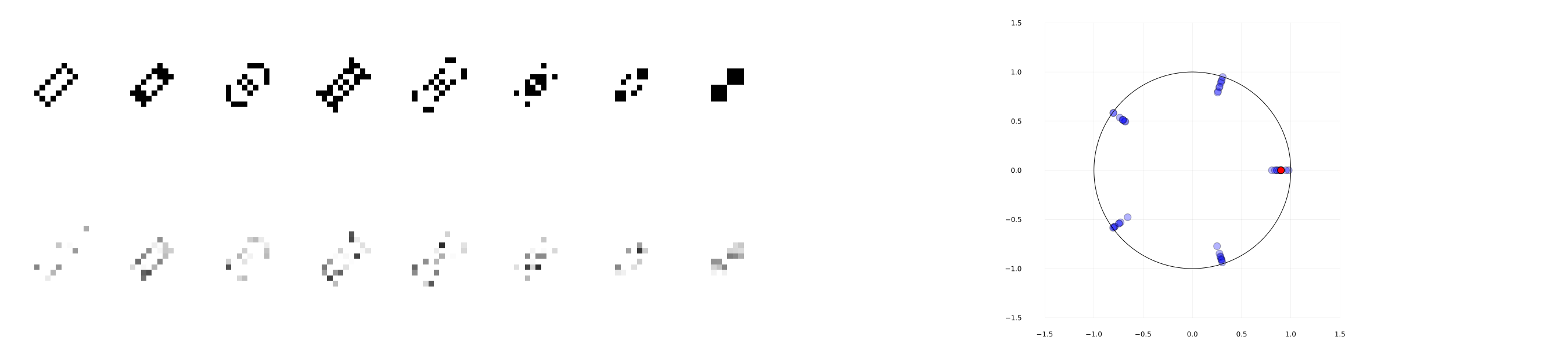
Figure 1: Left: Illustration of a period eight instance of LifeGame; (top) original transitions. (down) an instance of noised observation. Right: $\mu$-nearly periodic dynamics (5.1).

We use a specific instance of LifeGame which is illustrated in Figure 1. As shown on the top eight pictures, starting from certain configuration of cells, it shows transitions of period eight. The sample size is computed as the smallest integer satisfying (4.2), and the threshold $\varepsilon$ is given by (4.1). To prevent the dimension from becoming too large, we used five cells that correctly displays period eight, therefore $d=5$. Noise $\eta_{t}$ is given by i.i.d. Gaussian with proxy $R=0.3$, and the down eight pictures of Figure 1 are some instances of noised observations. We tested four different random seeds (i.e., 1234, 2345, 3456, 4567), and for all of them, the algorithm outputs the fundamental period eight.

Period estimation: Simple $\mu$-nearly periodic system.

We consider the following $\mu$-nearly periodic system that circulates over a circle with small variations:

$$r_{t+1}=\mu\left(\alpha\frac{r_{t}-1}{\mu}-\lceil\alpha\frac{r_{t}-1}{\mu}\rceil\right)+1,~{}~{}~{}~{}~{}\theta_{t+1}=\theta_{t}+\frac{2\pi}{L},$$ (5.1)

where $r$ and $\theta$ are radius and angle, $\alpha\notin\mathbb{Q}$. We use $\mu=0.001$, $L=5$, and $\alpha=\pi$. Noise $\eta_{t}$ is drawn i.i.d. from the uniform distribution within $[-R,R]$ for $R=0.3$. We tested four different random seeds (i.e., 1234, 2345, 3456, 4567), and for all of them, the algorithm outputs $\mu$-nearly period five.

Eigenvalue estimation: Permutation and shrink.

We use $d=5$, and $M\in\mathbb{R}^{5\times 5}$ is made such that 1) the first four dimensions are for permutation (i.e., each of row and column of $4\times 4$ sub-matrix has only one nonzero element that is one.), and 2) the last dimension is simply shrinking; we gave $0.7$ for $(5,5)$-element of $M$. Initial vector $\theta_{0}$ and each action $\tilde{x}_{m},~{}m\in[d],$ are uniformly sampled from the unit sphere in $\mathbb{R}^{5}$. The value $L$ is computed by $4!=24$. We used the smallest integer $N$ that satisfies (4.5), multiplied by $C_{\rm sim}$ for different $C_{\rm sim}>0$. The results are shown in Table 1; it is observed that the more samples we use the more accurate the estimates become to $(\theta_{0},1,5)$-distinct eigenvalue of $M^{5}$. Noise $\eta_{t}$ is drawn i.i.d. from the uniform distribution within $[-R,R]$ for $R=0.3$.

Table 1: Results for eigenvalue estimation. The top-most row shows the true eigenvalues of $M^{5}$, and the second row shows its $(\theta_{0},1,5)$-distinct eigenvalues. From the third to sixth row, it shows the estimated eigenvalues for different values of $C_{\rm sim}$.

eigenvalues of $M^{5}$	$1.000$	$1.000$	$-0.500-0.866i$	$-0.500+0.866i$	$0.168$
$(\theta_{0},1,d)$	$1.000$	$0$	$-0.500-0.866i$	$-0.500+0.866i$	$0$
when $C_{\rm sim}=1$	$1.000+0.008i$	$0$	$-0.489-0.860i$	$-0.510+0.869i$	$0$
when $C_{\rm sim}=5$	$0.999-0.000i$	$0$	$-0.495-0.867i$	$-0.501+0.862i$	$0$
when $C_{\rm sim}=10$	$1.000+0.003i$	$0$	$-0.497-0.867i$	$-0.501+0.864i$	$0$
when $C_{\rm sim}=30$	$1.000+0.001i$	$0$	$-0.500-0.866i$	$-0.500+0.864i$	$0$

6 Discussion and conclusion

This work proposed novel algorithms for estimating certain global information about the dynamical systems from bandit feedback contaminated by sub-Gaussian noise. The key contributions are the use of exponential sums and the definitions of novel terms, namely, aliquot nearly period and $(\theta,\lambda,k)$-distinct eigenvalues. We list a potentially important list of future works below.

Extensions to random dynamical systems and other forms of feedback: We conjecture that, under the condition that variance of trajectories generated by a random dynamical system (RDS) is sufficiently small, the similar estimation procedure is adopted for such RDS. Also, it is an interesting direction to study other dynamic structures such as the Lyapunov exponents for nonlinear systems.

Unified theory for learnability of dynamical structures: The proper use of exponential sums enables us to average out the noise while preserving particular information. Studying when this separation is feasible for different set of information, noise, and class of problems should be important.

Optimality of the results: Related to the above, we did not study if our sample complexity bound is what we can best achieve under our problem settings. Studying when it is necessary to employ our algorithms and if the sample complexity bound is tight should be further investigated.

Appendix A estimation of period for almost periodic sequence

Lemma A.1.

Let $\mathbf{a}:=(a_{j})_{j=1}^{\infty}$ be a sequence of $\mu$-nearly period $L$. Let

$$\sigma:=\sigma_{L}(\mathbf{a}):=\sup_{t_{0}\geq 1}\sqrt{\frac{1}{L}\sum_{t=t_{0}}^{t_{0}+L-1}\left|a_{t}-\frac{1}{L}\sum_{j=t_{0}}^{t_{0}+L-1}a_{j}\right|^{2}}.$$

Then, we have the following statements:

1. if $L>1$, then there exists $s\in\mathbb{Z}_{>0}$ with $s<L$ such that

   $$\left|\mathcal{R}\left((a_{j})_{j=1}^{T};s/L\right)\right|>\sqrt{\frac{\sigma^{2}-2\mu\sigma}{L}}-\mu-\frac{L\sup_{t\geq 1}|a_{t}|}{T},$$ (A.1)

2. $\beta$ is not a divisor of $L$, then for any $\alpha\in\mathbb{Z}_{>0}$,

   $$\left|\mathcal{R}\left((a_{j})_{j=1}^{T};\alpha/\beta\right)\right|<\mu+\frac{L^{2}\mathcal{C}_{0}(\mu+\sup_{t\geq 1}|a_{t}|)}{T}.$$ (A.2)

   where $\mathcal{C}_{0}:=1+{2}/{\sqrt{2}\pi(3/4)^{\pi^{2}/6}}=1.72257196806914...$.

Proof.

As $(a_{t})_{t=1}^{\infty}$ is $\mu$-almost periodic, there exist $(b_{t})_{t=1}^{\infty}$ of period $L$ and $(c_{t})_{t=1}^{\infty}$ with $\sup_{t\geq 1}|c_{t}|<\mu$ such that

$$a_{t}=b_{t}+c_{t}.$$

First, we prove (A.1). Let

$$\tilde{b} :=\frac{1}{L}\sum_{t=1}^{L}b_{t},$$

$$\hat{b}_{q} :=\frac{1}{L}\sum_{t=1}^{L}b_{t}e^{i2\pi tq},\quad(q\in\mathbb{Q}).$$

We claim that

$$L\cdot\sup\{|\hat{b}_{s/L}|^{2}\}_{s=1}^{L-1}>\sum_{s=1}^{L-1}|\hat{b}_{s/L}|^{2}=\frac{1}{L}\sum_{t=1}^{L}|b_{t}-\tilde{b}|^{2}\geq\sigma^{2}-2\mu\sigma.$$ (A.3)

In fact, the first inequality is obvious. The equality follows from the Plancherel formula for a finite abelian group (see, for example, [Serre, 1977, Excercise 6.2]). As for the last inequality, take arbitrary $t_{0}\in\mathbb{Z}_{>0}$ and define $\tilde{a}=L^{-1}\sum_{t=t_{0}}^{t_{0}+L-1}a_{t}$ and $\tilde{c}=L^{-1}\sum_{t=t_{0}}^{t_{0}+L-1}c_{t}$. Then, we have

$$\frac{1}{L}\sum_{t=1}^{L}|b_{t}-\tilde{b}|^{2} \geq\frac{1}{L}\sum_{t=t_{0}}^{t_{0}+L-1}|a_{t}-\tilde{a}|^{2}+\frac{1}{L}\sum_{t=t_{0}}^{t_{0}+L-1}|c_{t}-\tilde{c}|^{2}-\frac{2}{L}\sum_{t=t_{0}}^{t_{0}+L-1}|a_{t}-\tilde{a}|\cdot|c_{t}-\tilde{c}|$$

$$\geq\frac{1}{L}\sum_{t=t_{0}}^{t_{0}+L-1}|a_{t}-\tilde{a}|^{2}+\frac{1}{L}\sum_{t=t_{0}}^{t_{0}+L-1}|c_{t}-\tilde{c}|^{2}$$

$$\qquad-2\sqrt{\frac{1}{L}\sum_{t=t_{0}}^{t_{0}+L-1}|a_{t}-\tilde{a}|^{2}}\cdot\sqrt{\frac{1}{L}\sum_{t=t_{0}}^{t_{0}+L-1}|c_{t}-\tilde{c}|^{2}}$$

$$\geq\frac{1}{L}\sum_{t=t_{0}}^{t_{0}+L-1}|a_{t}-\tilde{a}|^{2}-2\mu\sigma.$$

Here, we used the Cauchy-Schwartz inequality in the second inequality. Since $t_{0}$ is arbitrary, we have (A.3). Let $s\in\mathrm{argmax}_{s=1,\dots,L-1}|\hat{b}_{s/L}|^{2}$ and let $q:=s/L$. Let $T=LT^{\prime}+\gamma$ for some $T^{\prime},\gamma\in\mathbb{N}$ with $0\leq\gamma<L$. Then, we have

$$\left|\mathcal{R}\left((a_{j})_{j=1}^{T};q\right)\right| \geq\left|\frac{1}{T^{\prime}}\sum_{t=0}^{T^{\prime}-1}\left[\frac{1}{L}\sum_{s=1}^{L}a_{Lt+s}e^{i2\pi qs}\right]\right|-\frac{L\sup_{t\geq 1}|a_{t}|}{T}$$

$$>|\hat{b}_{q}|-\mu-\frac{L\sup_{t\geq 1}|a_{t}|}{T}$$

$$\geq\sqrt{\frac{\sigma^{2}-2\mu\sigma}{L}}-\mu-\frac{L\sup_{t\geq 1}|a_{t}|}{T}.$$

Next, we prove (A.2). As in the same computation as above, we have

$$\left|\mathcal{R}\left((a_{j})_{j=1}^{T};\alpha/\beta\right)\right| \leq\frac{LT^{\prime}}{T}\left|\frac{1}{T^{\prime}}\sum_{t=0}^{T^{\prime}-1}e^{i2\pi\alpha Lt/\beta}\left[\frac{1}{L}\sum_{s=1}^{L}a_{Lt+s}e^{i2\pi\alpha s/\beta}\right]\right|+\frac{L\sup_{t>0}|a_{t}|}{T}$$

$$<\frac{LT^{\prime}}{T}\left|\frac{1}{T^{\prime}}\sum_{t=0}^{T^{\prime}-1}e^{i2\pi\alpha Lt/\beta}\right|\cdot\left|\frac{1}{L}\sum_{s=1}^{L}b_{s}e^{i2\pi\alpha s/\beta}\right|+\mu+\frac{L\sup_{t>0}|a_{t}|}{T}$$

$$<\frac{2}{\left|1-e^{i2\pi\alpha L/\beta}\right|}\cdot\left(\mu+\sup_{t\geq 1}|a_{t}|\right)\cdot\frac{L}{T}+\mu+\frac{L\sup_{t>0}|a_{t}|}{T}.$$

By Lemma D.1, we have

$$\left|\mathcal{R}\left((a_{j})_{j=1}^{T};\alpha/\beta\right)\right| <\left(\mu+\sup_{t\geq 1}|a_{t}|\right)\frac{2\beta L}{\sqrt{2}(3/4)^{\pi^{2}/6}T}+\mu+\frac{L\sup_{t\geq 1}|a_{t}|}{T}$$

$$<\mu+\frac{L\beta\mathcal{C}_{0}(\mu+\sup_{t\geq 1}|a_{t}|)}{T}.$$

∎

We provide a proof of Proposition 4.1.

Proof of Proposition 4.1.

$$B :=L_{\max}\sup_{t>0}|a_{t}|,$$

$$C :=\sqrt{4R^{2}\log(4/\delta)},$$

$$D :=L_{\max}^{2}\mathcal{C}_{0}\left(\mu+\sup_{t\geq 1}|a_{t}|\right).$$

Then, $\sqrt{T}>0$ satisfies the following inequality

$$\varepsilon \leq 2\varepsilon-\mu-\frac{L_{\max}\sup_{t>0}|a_{t}|}{T}-\sqrt{\frac{4R^{2}\log(4/\delta)}{T}},$$

$$\varepsilon \geq\mu+\frac{L_{\max}^{2}\mathcal{C}_{0}(\mu+\sup_{t\geq 1}|a_{t}|)}{T}+\sqrt{\frac{4R^{2}\log(4/\delta)}{T}},$$

if and only if

$$\sqrt{T}\geq\max\left\{\frac{C+\sqrt{C^{2}+4(\varepsilon-\mu)B}}{2(\varepsilon-\mu)},\frac{C+\sqrt{C^{2}+4(\varepsilon-\mu)D}}{2(\varepsilon-\mu)}\right\}.$$

Since $L_{\max}\geq 2$, $D\geq B$, $\mu<\gamma\sup_{t\geq 1}|a_{t}|$, $\mathcal{C}_{0}(1+\gamma)<3$, and

$$\varepsilon-\mu =\frac{\sigma_{0}(1-\lambda)}{\sqrt{L_{\max}}}\cdot\frac{\sqrt{L_{\max}}}{1+\sqrt{4L_{\max}+1}}$$

$$\geq\frac{\sigma_{0}(1-\lambda)}{2\sqrt{2}\sqrt{L_{\max}}},$$

$$\max\left\{\frac{C+\sqrt{C^{2}+4(\varepsilon-\mu)B}}{2(\varepsilon-\mu)},\frac{C+\sqrt{C^{2}+4(\varepsilon-\mu)D}}{2(\varepsilon-\mu)}\right\}$$

$$=\frac{C+\sqrt{C^{2}+4(\varepsilon-\mu)D}}{2(\varepsilon-\mu)}$$

$$\leq 2\sqrt{\frac{L_{\max}C^{2}}{4(\varepsilon-\mu)^{2}}+\frac{D}{(\varepsilon-\mu)}}$$

$$\leq 2\sqrt{\frac{2L_{\max}^{2}C^{2}}{\sigma_{0}^{2}(\xi-\lambda)^{2}}+\frac{6\sqrt{2}L_{\max}^{5/2}\sup_{t\geq 1}|a_{t}|}{\sigma_{0}(\xi-\lambda)}}$$

$$\leq 2\sqrt{\frac{2L_{\max}^{2}C^{2}}{\sigma_{0}^{2}(\xi-\lambda)^{2}}+\frac{9L_{\max}^{5/2}\sup_{t\geq 1}|a_{t}|}{\sigma_{0}(\xi-\lambda)}},$$

where we used the formula $\sqrt{1-2\gamma}=2\gamma\sqrt{L_{\max}}$. Since $2\varepsilon\leq\sqrt{(\sigma_{0}^{2}-2\mu\sigma_{0})/L_{\max}}$, the statement follows from Lemma A.1. ∎

Proof of Theorem 4.2.

Let $\mathscr{K}$ be the set of all combinations $(m,\beta,s,q)$ such that $m\in[d]$, $\beta\in[L_{\rm max}]$, $s\in\{0,1,\dots,\beta-1\}$ and $\{q=\alpha/\ell:\alpha\in\{1,\dots,\ell-1\}\}$. We remark that

$$|\mathscr{K}| \leq\sum_{m=1}^{d}\sum_{\beta=1}^{L_{\max}}\sum_{\alpha\leq L_{\max}/\beta}\sum_{\alpha=1}^{\ell-1}\sum_{s=0}^{\beta-1}1=d\sum_{\beta=1}^{L_{\max}}\sum_{\ell\leq L_{\max}/\beta}\beta(\ell-1)$$

$$\leq d\sum_{\beta=1}^{L_{\max}}\frac{L_{\max}}{2}\left(\frac{L_{\max}}{\beta}-1\right)$$

$$\leq\frac{dL_{\max}^{2}\log L_{\max}}{2}.$$

Also, let $\mathcal{E}^{T_{p}}_{\kappa}$ be the event such that, for the combination $\kappa\in\mathscr{K}$,

$$\left|\frac{1}{\lfloor T_{p}/\beta\rfloor}\sum_{j=0}^{\lfloor T_{p}/\beta\rfloor-1}\left\{\eta_{t_{0}+\beta j+s}e^{\frac{i2\pi\alpha j}{\ell}}\right\}\right|\leq\sqrt{\frac{4R^{2}\log\left(4dL_{\rm max}^{2}\log L_{\max}/\delta\right)}{\lfloor T_{p}/\beta\rfloor}}.$$

Because the error sequence satisfies conditionally $R$-sub-Gaussian, using Lemma D.2 and from the fact that any subsequence of the filtration $\{\mathcal{F}_{\tau}\}$ is again a filtration, we obtain, for each $\kappa\in\mathscr{K}$,

$$\mathrm{Pr}\left[\mathcal{E}^{T_{p}}_{\kappa}\right]\geq 1-\frac{\delta}{dL_{\rm max}^{2}\log L_{\max}}.$$

Define $\mathcal{E}^{T_{p}}:=\bigcap_{\kappa\in\mathscr{K}}\mathcal{E}^{T_{p}}_{\kappa}$. Then, it follows from the Fréchet inequality that

$$\mathrm{Pr}\left[\mathcal{E}^{T_{p}}\right] =\mathrm{Pr}\left[\bigcap_{\kappa\in\mathscr{K}}\mathcal{E}^{T_{p}}_{\kappa}\right]\geq|\mathscr{K}|\left(1-\frac{\delta}{dL_{\rm max}^{2}\log L_{\max}}\right)-(|\mathscr{K}|-1)$$

$$=1-\frac{\delta|\mathscr{K}|}{dL_{\rm max}^{2}\log L_{\max}}\geq 1-\delta.$$

Let $\widehat{L}$ be the output of Algorithm 1. We show that, with probability $1-\delta$, $\widehat{L}$ is $(\rho,\sqrt{d})$-anp of $L$. In fact, suppose $\widehat{L}$ is not $(\rho,\sqrt{d})$-anp. We note that $\widehat{L}<L$. There exists $s\in\{0,\dots,\widehat{L}-1\}$ and $t_{1},t_{2}\in\mathbb{Z}_{>0}$,

$$\|f^{s+\widehat{L}t_{1}}(\theta)-f^{s+\widehat{L}t_{2}}(\theta)\|>\rho+2\sqrt{d}\mu.$$

Let $m^{\prime}\in\mathrm{argmax}_{m=1,\dots,d}\left|f^{s+\widehat{L}t_{1}}(\theta)^{\top}\mathbf{u}_{m}-f^{s+\widehat{L}t_{2}}(\theta)^{\top}\mathbf{u}_{m}\right|$. Put $a_{t}:=f^{s+\widehat{L}t}(\theta)^{\top}\mathbf{u}_{m^{\prime}}$. Then, for any $t,t^{\prime}\in\mathbb{Z}_{>0}$, we have

$$|a_{t}-a_{t^{\prime}}| \geq|a_{t_{1}}-a_{t_{2}}|-2\mu$$

$$\geq\frac{\|f^{s+\widehat{L}t_{1}}(\theta)-f^{s+\widehat{L}t_{2}}(\theta)\|}{\sqrt{d}}-2\mu$$

$$>\frac{\rho}{\sqrt{d}}.$$

Thus, by definition, we have

$$\sigma_{L/\widehat{L}}((a_{t})_{t})\geq\frac{\rho}{2\sqrt{dL/\widehat{L}}}\geq\frac{\rho}{2\sqrt{dL_{\max}}}.$$

Let $\sigma_{0}=\rho/2\sqrt{dL_{\max}}$ and $\xi:=\gamma^{-1}/3\sqrt{L_{\max}}$. Then, $\mu/(\gamma\xi)<\sigma_{0}\leq\sigma_{L/\widehat{L}}((a_{t})_{t})$, and

$$\frac{8L_{\max}R^{2}\log(4/\delta)}{\sigma_{0}^{2}(\xi-\lambda)^{2}}+\frac{36L_{\max}^{5/2}\sup_{t\geq 1}|a_{t}|}{\sigma_{0}(\xi-\lambda)}$$

$$\leq\frac{32\xi^{-2}dL_{\max}^{2}R^{2}\log(4/\delta)}{\rho^{2}(1-r)^{2}}+\frac{72\xi^{-1}\sqrt{d}L_{\max}^{3}\sup_{t\geq 1}|a_{t}|}{\rho(1-r)}$$

$$\leq\frac{72dL_{\max}^{2}R^{2}\log(4/\delta)}{\rho^{2}(1-r)^{2}}+\frac{108\sqrt{d}L_{\max}^{3}\sup_{t\geq 1}|a_{t}|}{\rho(1-r)}.$$

The last inequality follows from $\xi\geq 2/3$. Thus, by Proposition 4.1, the algorithm finds $\beta>\widehat{L}$ in $m^{\prime}$-th loop, and the output becomes an integer larger than $\widehat{L}$, which is contradiction. ∎

Appendix B Eigenvalue estimation

Here, we provide the proof of Theorem 4.5.

Recall that $M\in\mathbb{R}^{d\times d}$ is a real matrix and there exists $\theta$ such that $(M^{t}\theta)_{t=t_{0}}^{\infty}$ is a $\mu$-nearly periodic sequence for some $t_{0}>0$. We define $\kappa\geq 1$ by

$$\kappa:={\inf_{P}{\left\{\|P\|\|P^{-1}\|:P^{-1}MP=J_{M}\right\}}},$$

where $J_{M}$ is a Jordan normal form of $M$. Also, we define $\Delta\in(0,1]$ to be a value such that $|\lambda|\leq 1-\Delta$ for any eigenvalue $\lambda$ of $M$ that satisifes $|\lambda|<1$.

Let $W$ be a linear subpace of $\mathbb{C}^{d}$ generated by the trajectory $\{M\theta,M^{2}\theta,\dots\}$ and denote its dimension by $d_{0}$. Note that restriction of $M$ to $W$ induces a linear map from $W$ to $W$. We denote by $M_{\theta}$ the induced linear map from $W$ to $W$. Let $W=\oplus_{\alpha\in\Lambda}W_{\alpha}$ be the decomposition via the generalized eigenspaces of $M_{\theta}$, where $\Lambda$ is the set of eigenvalues of $M_{\theta}$ and $W_{\alpha}:=\mathscr{N}((\alpha I-M_{\theta})^{d_{0}})$. Let $\mathbb{C}^{d}=\oplus_{\alpha}V_{\alpha}$ be the decomposition via generalized eigenspaces of $M$, where $\alpha$ runs over the eigenvalues of $M$ and $V_{\alpha}:=\mathscr{N}((\alpha I-M)^{d})$. We define

$$W_{=1}:=\oplus_{|\alpha|=1}W_{\alpha},$$

$$W_{<1}:=\oplus_{|\alpha|<1}W_{\alpha},$$

We note that $W=W_{=1}\oplus W_{<1}$ (see Proposition 3.2).

B.1 Proof of Proposition 3.2 and a corollary

Proof of Proposition 3.2.

We note that $M^{t}\theta$ is a nearly periodic sequence, in particular, a bounded sequence, thus, $\{M^{t}v\}_{t\geq 1}$ is also bounded for any $v\in W$ as $v$ is a linear combination of finite elements in $\{M^{t}\theta\}_{t\geq 1}$. First, we show that an eigenvalue $\alpha$ with $\theta_{\alpha}\neq 0$ satisfies $|\alpha|\leq 1$. An eigenvector $w$ of $\alpha$ is contained in $W$. Thus, we conclude that $|\alpha|\leq 1$. Next, we show the second statement. Suppose $(M-\alpha I)\theta_{\alpha}\neq 0$. Since $(M-\alpha I)^{d}\theta_{\alpha}=0$, there exists $1<d^{\prime}<d$ such that $(M-\alpha I)^{d^{\prime}+1}\theta_{\alpha}=0$ but $(M-\alpha I)^{d^{\prime}}\theta_{\alpha}\neq 0$. Let $w^{\prime}:=(M-\alpha I)^{d^{\prime}-1}\theta_{\alpha}$. Then, we see that $(M-\alpha I)^{2}w^{\prime}=0$ but $(M-\alpha I)w^{\prime}\neq 0$. By direct computation, we see that

$$\|M^{t}w^{\prime}\|=\|(M-\alpha I+\alpha I)^{t}w^{\prime}\|\geq t\|(M-\alpha I)w^{\prime}\|-\|w^{\prime}\|.$$

Thus, we see that $\|M^{t}w^{\prime}\|\to\infty$ as $t\to\infty$, which contradicts the fact that $\{M^{t}w^{\prime}\}$ is a bounded sequence. The last statement is obvious. ∎

We have the following statement as a corollary of Proposition 3.2:

Corollary B.1.

There exist linear maps $M_{1},M_{<1}:W\to W$ such that

1. $M_{\theta}=M_{1}+M_{<1}$,

2. $M_{1}M_{<1}=M_{<1}M_{1}=O$,

3. $M_{1}$ is diagonalizable and any eigenvalue of $M_{1}$ is of magnitude $1$, and

4. any eigenvalue of $M_{<1}$ is of magnitude smaller than $1$.

Proof.

Let $p:W\to W_{=1}$ be the projection and let $i:W_{=1}\to W$ be the inclusion map. We define $M_{1}:=iM_{\theta}p$. We can construct $M_{<1}$ in the similar manner and these matrices are desired ones. ∎

B.2 Proof of Proposition 4.4

First, we introduce the Weyl sum:

Lemma B.2 (Lower bound on Weyl sum [Bourgain, 1993, Oh, ]).

Define the Weyl sum by

$$\mathscr{W}(N,b,q):=\sum_{j=0}^{N}e^{i2\pi\left(j\frac{2b}{4q}+j^{2}\frac{1}{4q}\right)},$$

for some $b\in\mathbb{N},~{}q\in\mathbb{Z}_{>0},~{}b<q$ and $N\in\mathbb{Z}_{>0}$. Then, for $N\geq 16q^{2}$, it holds that

$$|\mathscr{W}(N,b,q)|\in\Omega\left(\frac{N}{\sqrt{q}}\right).$$

Proof.

It is immediate from Proposition 3.1 in [Oh, ] because ${\rm gcd}(1,4q)=1$, $4q\equiv 0\mod 4$, and $2b$ is even. ∎

We define $C_{\rm ws}(L)>0$ by

$$C_{\rm ws}(L):=\inf\left\{C>0:C^{-1}<\left|\frac{1}{N}\mathscr{W}(N,b,L)\right|<C\text{ for any }N\geq 16L^{2},0\leq b<L\right\}.$$

We provide a generalized result of Proposition 4.4. The matrix $Q_{N}$ in Proposition 4.4 corresponds to $Q_{N}(M_{1})$ defined below.

Proposition B.3.

Let $M_{1}$ and $M_{<1}$ be matrices as in Corollary B.1. We define linear maps on $W$ by

$$Q_{N}(M_{1}) :=\mathscr{W}\left((M_{1}^{2d^{2}j})_{j=0}^{N-1}\right)$$

$$Q_{N}(M_{<1}) :=\mathscr{W}\left((M_{<1}^{2d^{2}j})_{j=0}^{N-1}\right).$$

Then, we have the following statement:

1. $\mathscr{W}\left((M_{\theta}^{2d^{2}j})_{j=0}^{N-1}\right)=Q_{N}(M_{1})+Q_{N}(M_{<1})$,

2. for any $N\geq 16L^{2}$, $Q_{N}(M_{1})$ is invertible on $W_{=1}$,

3. for any $r\geq 0$ and for any $N\geq 16L^{2}$, $\|M_{1}^{r}Q_{N}(M_{1})|_{W_{=1}}\|,\|(M_{1}^{r}Q_{N}(M_{1}))|_{W_{=1}}^{-1}\|\leq\kappa C_{\rm ws}(L)$,

4. for any $r\geq 2(d-1)$, we have

   $$\|M_{<1}^{r}Q_{N}(M_{<1})\|\leq\frac{d^{2}\kappa e^{-\Delta(r-d+1)}}{N\Delta^{d-1}}.$$

Proof.

We prove 1. By the property 1 and 2 in Corollary B.1, we have $\mathscr{W}((M^{2d^{2}j})_{j=0}^{N-1})=Q_{N}(M_{1})+Q_{N}(M_{<1})$. Next, we prove 2. When we regard $Q_{N}(M_{1})|_{W_{=1}}$ as a linear map on $W_{=1}$, it is represented as a diagonal matrix ${\rm diag}(\mathscr{W}(N,b_{1},L),\dots,\mathscr{W}(N,b_{m},L))$, where $m={\rm dim}W_{=1}$. Therefore, by Lemma B.2, $Q_{N}(M_{1})$ is a bijective linear map on $W_{=1}$. Next, we prove 3. We estimate $\|M_{1}^{r}Q_{N}(M_{1})\|$. Let $p:\mathbb{C}^{d}\to W$ be the orthogonal projection and let $i:W\to\mathbb{C}^{d}$ be the inclusion map. Let $\tilde{M}_{1}:=iM_{1}p\in\mathbb{C}^{d\times d}$. Then, we have

$$\|Q_{N}(M_{1})\|=\|Q_{N}(\tilde{M}_{1})\|\leq\kappa C_{\rm ws}(L).$$

Next, we estimate $\|M_{<1}^{r}Q_{N}(M_{<1})\|$. Let $\tilde{M}_{<1}:=iM_{<1}p$. Then, $iM_{<1}^{r}Q_{N}(M_{<1})p=\mathscr{W}((\tilde{M}_{<1}^{2d^{2}j+r})_{j=0}^{N-1})$ and $\|iM_{<1}^{r}Q_{N}(M_{<1})p\|=\|M_{<1}^{r}Q_{N}(M_{<1})\|$. Let $P$ be a regular matrix such that

$$\tilde{M}_{<1}=PJP^{-1},$$

where $J$ is the Jordan normal form. Then, for $r\geq 2(d-1)$, we see that

$$\|M_{<1}^{r}Q_{N}(M_{<1})\| =\|iM_{<1}^{r}Q_{N}(M_{<1})p\|$$

$$\leq\frac{\kappa}{N}\sum_{j=0}^{N-1}\|J^{2d^{2}j+r}\|$$

$$\leq\frac{d^{2}\kappa}{N}\sum_{j=0}^{N-1}\binom{2d^{2}j+r}{d-1}(1-\Delta)^{2d^{2}j+r-d+1}$$

$$<\frac{d^{2}\kappa}{N}\sum_{j=0}^{\infty}\binom{2d^{2}j+r}{d-1}(1-\Delta)^{2d^{2}j+r-d+1}$$

$$\leq\frac{d^{2}\kappa(1-\Delta)^{r-d+1}}{N\Delta^{d-1}}\leq\frac{d^{2}\kappa e^{-\Delta(r-d+1)}}{N\Delta^{d-1}}.$$

The second last inequality is proved as follows: for $|a|<1$, $n\geq 1$ and $r\geq m\geq 0$,

$$\left|\sum_{j=0}^{\infty}\binom{nj+r}{m}a^{nj-m+r}\right| =\left|\left.\frac{1}{m!}\frac{d^{m}}{dx^{m}}\sum_{j=0}^{\infty}x^{nj+r}\right|_{x=a}\right|$$

$$=\frac{1}{m!}\left|\left.\frac{d^{m}}{dx^{m}}\frac{x^{r}}{1-x^{n}}\right|_{x=a}\right|$$

$$\leq\frac{1}{m!}\sum_{j=0}^{m}\binom{m}{j}\frac{r!}{(r-m+j)!}|a|^{r-m+j}\left|\left.\frac{d^{j}}{dx^{j}}\frac{1}{1-x^{n}}\right|_{x=a}\right|$$

$$\leq\frac{1}{m!}\sum_{j=0}^{m}\binom{m}{j}\frac{r!}{(r-m+j)!}\frac{j!|a|^{r-m+j}}{(1-|a|)^{j}}=\sum_{j=0}^{m}\binom{r}{j}\frac{|a|^{r-m+j}}{(1-|a|)^{j}},$$

where, the last inequality follows from

$$\left|\frac{d^{m}}{dx^{m}}\frac{1}{1-x^{n}}\right|=\left|\sum_{\zeta^{n}=1}\frac{m!\zeta^{1-n}}{n(\zeta-x)^{m}}\right|\leq\frac{m!}{(1-|x|)^{m}}.$$

Thus, we have

$$\sum_{j=0}^{m}\binom{r}{j}\frac{|a|^{r-m+j}}{(1-|a|)^{j}}\leq|a|^{r-m}\sum_{j=0}^{r}\binom{r}{j}\left(\frac{|a|}{1-|a|}\right)^{j}\leq\frac{|a|^{r-m}}{(1-|a|)^{m}}.$$

∎

B.3 Proof of Theorem 4.5

Let

$$K :=(M\theta,\dots,M^{d}\theta):\mathbb{C}^{d}\to W,$$

$$E_{s}(N) :=\mathscr{W}\left((E_{s,j})_{j=0}^{N-1}\right):\mathbb{C}^{d}\to\mathbb{C}^{d}.$$

For a linear map $\mathcal{M}:W\to W$, we define linear maps:

$$X(\mathcal{M}) :=\left(\begin{array}[]{c}\tilde{x}_{1}^{\top}\mathcal{M}^{1}\\ \tilde{x}_{1}^{\top}\mathcal{M}^{2d+1}\\ \vdots\\ \tilde{x}_{d}^{\top}\mathcal{M}^{2(d-1)d+1}\end{array}\right):W\to\mathbb{C}^{d},$$

$$Q_{N}(\mathcal{M}) :=\mathscr{W}\left((\mathcal{M}^{2d^{2}j})_{j=0}^{N-1}\right):W\to W.$$

For $s=0,1$, we define linear maps on $\mathbb{C}^{d}$ by

$$A_{s}(N;\mathcal{M}) :=X(\mathcal{M})Q_{N}(\mathcal{M})\mathcal{M}^{sd+N-1}K+E_{s}(N),$$

$$B_{s}(N;\mathcal{M}) :=X(\mathcal{M})Q_{N}(\mathcal{M})\mathcal{M}^{sd+N-1}K.$$

We note that $A_{s}(N;M_{\theta})$ is identical to $A_{s}(N)$ defined in (4.4). We impose the following assumption on $X(M_{\theta})$:

Assumption 5.

The kernel of the linear map $X(M_{1})$ is the same as $\mathcal{N}(M_{1})$.

Note that this assumption holds with probability 1 if we randomly choose $\tilde{x}_{1},\dots,\tilde{x}_{d}$ (see Lemma B.10).

The following lemma provides an explicit description of $B_{0}(N;M_{1})^{\dagger}$.

Lemma B.4.

Suppose Assumption 5. Assume $N\geq 16L^{2}$. Let

$$U_{1} :=\mathscr{I}(B_{0}(N;M_{1}))\subset\mathbb{C}^{d},$$

$$U_{2} :=\mathscr{N}(B_{0}(N;M_{1}))\subset\mathbb{C}^{d},$$

$$U_{3} :=\mathscr{I}(M_{1})=W_{=1}\subset W.$$

Let $i:U_{1}\to\mathbb{C}^{d}$ be the inclusion map and $p:\mathbb{C}^{d}\to U_{2}^{\perp}$ the orthogonal projection. Then, restriction of $X(M_{1})$ (resp. $M_{1}K$) to $U_{3}$ (resp. $U_{2}^{\perp}$) induces an isomorphism on to $U_{1}$ (resp. $U_{3}$). If we denote the isomorphism by $\tilde{X}$ (resp, $\tilde{K}$). Then, $B_{0}(N;M_{1})^{\dagger}$ is given by

$$B_{0}(N;M_{1})^{\dagger}=p^{*}\tilde{K}^{-1}M_{1}|_{U_{3}}^{2-N}Q_{N}(M_{1})|_{U_{3}}^{-1}\tilde{X}^{-1}i^{*}.$$

Proof.

Since we have $\mathscr{N}(M_{1})=\mathscr{N}(M_{1}^{r+1})$ for all $r\geq 0$ and Assumption 5, surjectivity of $K$ by Proposition B.8, and bijectivity of $Q_{N}(M_{1})$ on $U_{3}$ by Proposition B.3, we have

$$U_{1} =\mathscr{I}(X(M_{1})|_{U_{3}}),$$

$$U_{2} =\mathscr{N}(M_{1}K).$$

Thus, the restriction of $X(M_{1})$ (resp. $K$) to $U_{3}$ (resp. $U_{2}^{\perp}$) induces an isomorphism onto $U_{1}$ (resp. $U_{3}$). Let us denote the isomorphism by $\tilde{X}$ (resp. $\tilde{K}$). Then, the last statement follows from Proposition B.7. ∎

Lemma B.5.

Assume $N\geq 16L^{2}$. Let

$$A:=B_{1}(N;M_{1})B_{0}(N;M_{1})^{\dagger}.$$

Then, $A$ is independent of $N$ and its eigenvalues are zeros except for $(\theta,1,d)$-distinct eigenvalues of $M$.

Proof.

We use the notation as in Lemma B.4. By Lemma B.4, we obtain

$$B_{1}(N;M_{1})B_{0}(N;M_{1})^{\dagger}=i\tilde{X}M_{1}^{d}\tilde{X}^{-1}i^{*},$$

which is independent of $N$ and its eigenvalues are zeros except for $(\theta,1,d)$-distinct eigenvalues of $M$. ∎

The following result will be used in the proof of Theorem 4.5 (but not essential).

Lemma B.6.

We have

$$\|X(M_{1})\| \leq\kappa\sqrt{d},$$

$$\|X(M_{<1})\| \leq\kappa(d+1)2^{d}.$$

Proof.

Considering the Jordan normal form, the first inequality is obvious. As for the second inequality, we define $J\in\mathbb{R}^{d\times d}$ by the nilpotent matrix

$$J:=\left(\begin{array}[]{cccc}0&1&&O\\ &\ddots&\ddots&\\ &&&1\\ O&&&0\end{array}\right).$$

Then, we have

$$\kappa^{-1}\|X(M_{1})\| \leq\sum_{r=1}^{d}\|(I+J)\|_{1}$$

$$=\sum_{r=1}^{d}\sum_{j=0}^{d}\binom{r}{j}(d-j)$$

$$=\sum_{j=0}^{d}(d-j)\sum_{r=1}^{d}\binom{r}{j}$$

$$=d+\sum_{j=1}^{d}(d-j)\sum_{r=1}^{d}\binom{r}{j}$$

$$=d+\sum_{j=1}^{d}(d-j)\binom{r+1}{j+1}$$

$$=d+(d+1)2^{d}-(d+1)d-(d+1)$$

$$<(d+1)2^{d}.$$

∎

Proof of Theorem 4.5.

Let $A$ be the matrix introduced in Lemma B.5. Let

$$\gamma(N):=\frac{\sqrt{4d^{2}R^{2}\log(4d^{2}/\delta)}+1}{\sqrt{N}}.$$

Let $M_{1}$ and $M_{<1}$ be matrices as in Corollary B.1. Then, by Proposition 3.2, we see that

$$A_{s}(N,M) =A_{s}(N,M_{1})+A_{s}(N,M_{<1}),$$

$$B_{s}(N,M) =B_{s}(N,M_{1})+B_{s}(N,M_{<1}).$$

We denote by $\hat{A}_{s}(N;M)$ (resp, $\hat{B}_{s}(N;M)$) the lower rank approximation via the singular value threshold $\gamma(N)$ (see Definition B.1). By direct computation, we have

$$\|A-A_{1}(N;M)\hat{A}_{0}(N;M)^{\dagger}\|$$

$$\leq\|A_{1}(N;M)\|\cdot\|\hat{A}_{0}(N;M)^{\dagger}-B_{0}(N;M_{1})^{\dagger}\|+\|A_{1}(N;M)-B_{1}(N;M_{1})\|\cdot\|B_{0}(N;M_{1})^{\dagger}\|$$

$$\leq(\|B_{1}(N;M_{1})\|+\|B_{1}(N;M_{<1})\|+\|E_{1}(N)\|)\cdot\|\hat{A}_{0}(N;M)^{\dagger}-B_{0}(N;M_{1})^{\dagger}\|$$

$$\qquad+\|B_{1}(N;M_{<1})+E_{1}(N)\|\cdot\|B_{0}(N;M_{1})^{\dagger}\|.$$

By Proposition B.3, for $s=0,1$ and for $N\geq\max\{2d,16L^{2}\}$, we have

$$\|B_{s}(N;M_{1})\| \leq\|X(M_{1})\|\cdot\|M_{1}^{N+sd-1}Q_{N}(M_{1})\|\cdot\|K\|$$

$$\leq\kappa C_{\rm ws}(L)\|X(M_{1})\|\|K\|$$

$$\leq Bd\kappa^{2}C_{\rm ws}(L)$$

$$\|B_{s}(N;M_{<1})\| \leq\|X(M_{<1})\|\cdot\|M_{<1}^{N+sd-1}Q_{N}(M_{<1})\|\cdot\|K\|$$

$$\leq\|X(M_{<1})\|\cdot\|K\|\cdot\frac{d^{2}\kappa e^{-\Delta(N+sd-d)}}{N\Delta^{d-1}}$$

$$\leq B\kappa\sqrt{d}(d+1)2^{d}\cdot\frac{d^{2}\kappa e^{-\Delta(N+sd-d)}}{N\Delta^{d-1}}$$

$$\leq\frac{B\kappa^{2}e^{d+6-\Delta(N+sd-d)}}{N\Delta^{d-1}},$$

where we used $\|K\|\leq\sqrt{d}B$ (Assumption 3), and $\|X(M_{<1})\|\leq\kappa(d+1)2^{d}$ (Lemma B.6), and $\sqrt{d}(d+1)d^{2}2^{d}<e^{d+6}$. By Lemma B.4 with Proposition B.3, we see that

$$\|B_{0}(N;M_{1})^{\dagger}\|\leq\kappa C_{\rm ws}(L)\|\tilde{X}^{-1}\|\cdot\|\tilde{K}^{-1}\|.$$

By using Lemma D.2 and union bounds, we obtain

$$\max(\|E_{1}(N)\|_{F},\|E_{2}(N)\|_{F})\leq\gamma(N)-\frac{1}{\sqrt{N}},$$

with probability at least $1-\delta$. Assume that

$$N\geq\frac{-(d-1)\log\Delta}{\Delta}+\frac{\log(B\kappa^{2})+d+6}{\Delta}+d.$$

Then, we see that $\|B_{s}(N;M_{<1})\|\leq 1/N$. Thus, by Lemma B.9, with probability at least $1-\delta$, we have

$$\|\hat{A}_{0}(N;M)^{\dagger}-B_{0}(N;M_{1})^{\dagger}\| \leq 8(\|E_{0}(N)\|+\|B_{0}(N;M_{<1})\|)\cdot\|B_{0}(N,M_{1})^{\dagger}\|^{2}(\sqrt{d}+1)$$

$$\leq 8\gamma(N)\cdot\|B_{0}(N,M_{1})^{\dagger}\|^{2}(\sqrt{d}+1)$$

$$\leq 8(1+\sqrt{d})\kappa^{2}C_{\rm ws}(L)^{2}\|\tilde{X}^{-1}\|^{2}\cdot\|\tilde{K}^{-1}\|^{2}\gamma(N).$$

Therefore, there exists $C>0$ depending on $\|X(M)\|$, $\|K\|$, $\kappa$, $C_{\rm ws}(L)$, $\|\tilde{X}^{-1}\|$, $\|\tilde{K}^{-1}\|$, and $d$ such that

$$\|A-A_{1}(N;M)\hat{A}_{0}(N;M)^{\dagger}\|<C\left(\frac{R^{2}\left(\log\left(1/\delta\right)+1\right)+1}{\sqrt{N}}\right),$$

with probability at least $1-\delta$. ∎

B.4 Miscellaneous

Definition B.1.

Let $A{\,:\,}\mathbb{R}^{m\times n}$ be a matrix. Let

$$A=U\left(\begin{array}[]{cc}D&O\\ O&O\end{array}\right)V^{*}$$

be a singular valued decomposition of $A$ where $U\in\mathbb{R}^{n\times n}$ and $V\in\mathbb{R}^{m\times m}$ are orthogonal matrices and $D:={\rm diag}(\sigma_{1},\dots,\sigma_{r})$ is a diagonal matrix with nonnegative components. Let $\gamma>0$. We define a low rank approximation $A_{\gamma}$ of $A$ via the singular value threshold $\gamma$ by the matrix $A_{\gamma}$ defined by

$$A_{\gamma}=U\left(\begin{array}[]{cc}D_{\gamma}&O\\ O&O\end{array}\right)V^{*},$$

where, $D_{\gamma}:={\rm diag}(\mathbf{1}_{[\gamma,\infty)}(\sigma_{1})\sigma_{1},\dots,\mathbf{1}_{[\gamma,\infty)}(\sigma_{r})\sigma_{r})$ and $\mathbf{1}_{I}$ is defined to be the characteristic function supported on $I\subset\mathbb{R}$.

We provide an expression of Moore-Penrose pseudo inverse:

Proposition B.7.

Let $A:\mathbb{C}^{m}\to\mathbb{C}^{n}$ be a linear map. Let $i:\mathscr{I}(A)\to\mathbb{C}^{n}$ be the inclusion map and let $p:\mathbb{C}^{m}\to\mathscr{N}(A)^{\perp}$ be the orthogonal projection. Let $\tilde{A}:=A|_{\mathscr{N}(A)}:\mathscr{N}(A)^{\perp}\to\mathscr{I}(A)$ be an isomorphism. Then, the Moore-Penrose pseudo inverse $A^{\dagger}$ coincides with $i^{*}\tilde{A}^{-1}p^{*}$.

Proof.

Let $B:=p^{*}\tilde{A}^{-1}i^{*}$. We remark that $A=i\tilde{A}p$, $i^{*}i={\rm id},pp^{*}={\rm id}$, we see that $ABA=A$, $BAB=B$, $(AB)^{*}=AB$, and $BA=(BA)^{*}$. By the uniqueness of Moore-Penrose pseudo inverse, $B=A^{\dagger}$. ∎

Proposition B.8.

Let $A\in\mathbb{C}^{d\times d}$ be a matrix and let $v\in\mathbb{C}^{d}$ be a vector. Let $V\subset\mathbb{C}^{d}$ be a linear subspace generated by $\{A^{j}v\}_{j=1}^{\infty}$. Then, $V=\mathscr{I}\left(Av,A^{2}v,\dots,A^{d}v\right)$.

Proof.

Put $W=\mathscr{I}\left((Av,A^{2}v,\dots,A^{d}v)\right)$. The inclusion $W\subset V$ is obvious, we prove the opposite inclusion. It suffices to show that $A^{j}v\in W$ for any positive integer $j>d$. By the Cayley-Hamilton theorem, $A^{d}=\sum_{j=1}^{d}c_{j}A^{d-j}$ for some $c_{j}\in\mathbb{C}$. Thus, by induction $A^{j}$ is a linear combination of $A,A^{2},\dots,A^{d}$, namely, $A^{j}v\in W$. ∎

We give several lemmas here.

Lemma B.9 (Perturbation bounds of the Moore-Penrose inverse).

Suppose $A\in\mathbb{C}^{d\times d}$ is a matrix. Let $E\in\mathbb{C}^{d\times d}$ be a matrix satisfying

$$\exists C>0,~{}~{}\forall N\in\mathbb{Z}_{>0},~{}~{}\|E\|\leq C\frac{1}{\sqrt{N}},$$

and let $\hat{A}_{E}\in\mathbb{C}^{d\times d}$ be the low rank approximation of $A+E$ via SVD with the singular value threshold $C/\sqrt{N}$. Then, we obtain

$$\left\|A^{\dagger}-\hat{A}_{E}^{\dagger}\right\|\leq\frac{8C\|A^{\dagger}\|^{2}\left(\sqrt{d}+1\right)}{\sqrt{N}}.$$

Proof.

Let $\sigma_{\min}=\|A^{\dagger}\|^{-1}$ be the minimal singular value of $A$. From [Meng and Zheng, 2010, Theorem 1.1] (or originally [Wedin, 1973]) and from the fact

$$\left\|\hat{A}_{E}-A\right\|\leq\|E\|+\frac{\sqrt{d}C}{\sqrt{N}},$$

we obtain

$$\left\|A^{\dagger}-\hat{A}_{E}^{\dagger}\right\|\leq\frac{1+\sqrt{5}}{2}\max\left\{\left\|A^{\dagger}\right\|^{2},\left\|\hat{A}_{E}^{\dagger}\right\|^{2}\right\}\left(\sqrt{d}+1\right)\frac{C}{\sqrt{N}}.$$

For $N$ such that $1\leq N\leq 4C^{2}/\sigma_{\rm min}^{2}$, we have $\left\|\hat{A}_{E}^{\dagger}\right\|\leq\sqrt{N}/C\leq 2/\sigma_{\rm min}$. Suppose singular values $\sigma_{k},~{}k\in[d]$, of $A$, and $\hat{\sigma}_{k},~{}k\in[d]$, of $A+E$ are sorted in descending order. Then, it holds that

$$|\sigma_{k}-\hat{\sigma}_{k}|\leq\left\|E\right\|.$$

Therefore, for $N>4C^{2}/\sigma_{\rm min}^{2}$, the minimum singular value $\hat{\sigma}_{d}$ is greater than $\sigma_{\rm min}/2$. In this case, $\hat{A}_{E}=A+E$, and it follows that $\left\|\hat{A}_{E}^{\dagger}\right\|\leq 2/\sigma_{\rm min}$. Hence, for all $N\geq 1$, we obtain

$$\left\|\hat{A}_{E}^{\dagger}\right\|\leq\frac{2}{\sigma_{\rm min}},$$

from which, it follows that

$$\left\|A^{\dagger}-\hat{A}_{E}^{\dagger}\right\|\leq\frac{2C\left(1+\sqrt{5}\right)\left(\sqrt{d}+1\right)}{\sigma_{\rm min}^{2}\sqrt{N}}\leq\frac{8C\|A^{\dagger}\|^{2}\left(\sqrt{d}+1\right)}{\sqrt{N}}.$$

∎

Lemma B.10 (Null space of random matrix).

Suppose $M_{k}\in\mathbb{R}^{d\times d},~{}k\in[d]$, have the same null space. Then, the null space of

$$X :=\left(\begin{array}[]{c}x_{1}^{\top}M_{1}\\ x_{2}^{\top}M_{2}\\ \vdots\\ x_{d}^{\top}M_{d}\\ \end{array}\right),$$ (B.5)

where $x_{k},~{}k\in[d]$, are independently drawn unit vector from the uniform distribution over the unit hypersphere, is the same as those of $M_{k}$ with probability one.

Proof.

Given any $k-1$ dimensional linear subspace in $\mathscr{N}(M_{k})^{\perp}$ for any $k\in[d]$, it holds that the probability that $x_{k}^{\top}M_{k}$ lies on that space is zero. Therefore, by union bound, and by the fact that the row space is the orthogonal complement of the null space, we obtain the result. ∎

Appendix C Reconstruction of original eigenvalues

Here, we use notation as in Section 4.2 and describe a procedure to reconstruct the $(\theta,1,d)$-distinct eigenvalues of $M$ via Algorithm 2.

Fix non-negative integer $r\geq 0$. Take $d+r$ random unit vectors $\tilde{x}_{1},\dots,\tilde{x}_{d+r}$. Then, for $s=0,1$, we may define a matrix $A_{s}(N;r)\in\mathbb{C}^{(d+r)\times(d+r)}$ so that its $(k,\ell)$ element is given by

$$\sum_{j=0}^{N-1}r_{2(k-1)(d+r)+s(d+r)+2(d+r)^{2}j+N+\ell}(\tilde{x}_{k})e^{\frac{i2\pi j^{2}}{4L}}.$$

Then, we see that Algorithm 2 outputs a matrix $\tilde{A}(r)$ that well approximates the $(\theta,1,d+r)$-distinct eigenvalues of $M$ since the matrix $A_{s}(N;r)$ coincides with $A_{s}(N)$ in the case when we replace $M$ and $\theta$ with $M(r)$ and $\theta(r)$ defined by

$$M(r) :=\left(\begin{array}[]{cc}M&O\\ O&O\end{array}\right)\in\mathbb{C}^{(d+r)\times(d+r)},$$

$$\theta(r) :=\left(\begin{array}[]{c}\theta\\ 0\\ \vdots\\ 0\end{array}\right)\in\mathbb{C}^{d+r}.$$

Let $r$ be an integer such that $r+d$ is prime $L$ and fix a positive integer $m$ such that $m(r+d)\equiv 1\mod L$. Then, the eigenvalues of $\tilde{A}(r)^{m}$ is close to those of $(\theta,1,1)$-distinct eigenvalues if we take sufficiently large $N$.

Appendix D Technical Lemmas

Lemma D.1.

For all $a\in(0,1)$, the following upper bound holds:

$$\left|\frac{1}{1-e^{i2\pi a}}\right|\leq\frac{1}{\sqrt{2}(1-a^{2})^{\pi^{2}/6}a}.$$

In particular, for any distinct $\alpha,\beta\in\mathbb{Z}_{>0}$ we have

$$\left|\frac{1}{1-e^{i2\pi\alpha/\beta}}\right|\leq\frac{\beta}{\sqrt{2}(3/4)^{\pi^{2}/6}}.$$

Proof.

The second statement immediately follows from the first inequality. The first inequality is a direct consequence of [Chesneau and Bagul, 2020, Proposition 3.2]. ∎

Lemma D.2 (Azuma-Hoeffding for exponential sum).

Let $\{X_{j}\}_{j=1}^{n}$ for $n\in\mathbb{Z}_{>0}$ be sub-Gaussian martingale difference with variance proxy $R^{2}$ and a filtration $\{\mathcal{F}_{j}\}$. Also, let $\{a_{j}\}\subset\mathbb{C}$ be a sequence of complex numbers satisfying $|a_{j}|\leq 1$ for all $j\in[n]$. Then, the followings hold, where $*[\cdot]$ stands for $\mathfrak{Re}[\cdot]$ or $\mathfrak{Im}[\cdot]$.

$$\mathrm{Pr}\left[\frac{1}{n}\left|*\left[\sum_{j=1}^{n}a_{j}X_{j}\right]\right|\leq\sqrt{\frac{2R^{2}\log\left(2/\delta\right)}{n}}\right]\geq 1-\delta$$

$$\mathrm{Pr}\left[\frac{1}{n}\left|\sum_{j=1}^{n}a_{j}X_{j}\right|\leq\sqrt{\frac{4R^{2}\log\left(4/\delta\right)}{n}}\right]\geq 1-\delta.$$

Proof.

For a filtration $\{\mathcal{F}\}_{i\leq n}$, we have

$$\mathbb{E}\left[e^{\lambda\mathfrak{Re}\left[\sum_{j=1}^{n}a_{j}X_{j}\right]}\right]\leq\mathbb{E}\left[e^{\lambda\mathfrak{Re}\left[\sum_{j=1}^{n-1}a_{j}X_{j}\right]}\mathbb{E}\left[e^{\lambda\mathfrak{Re}\left[a_{n}X_{n}\right]}\big{|}\mathcal{F}_{n-1}\right]\right]\leq e^{\frac{\lambda^{2}R^{2}}{2}}\mathbb{E}\left[e^{\lambda\mathfrak{Re}\left[\sum_{j=1}^{n-1}a_{j}X_{j}\right]}\right],$$

where the first inequality follows from the assumption of filtration, and the second inequality follows from

$$\mathbb{E}\left[e^{\lambda\mathfrak{Re}\left[a_{n}X_{n}\right]}\big{|}\mathcal{F}_{n-1}\right]=\mathbb{E}\left[e^{\lambda X_{n}\mathfrak{Re}\left[a_{n}\right]}\big{|}\mathcal{F}_{n-1}\right]\leq e^{\frac{\lambda^{2}R^{2}}{2}}.$$

By induction, we obtain

$$\mathbb{E}\left[e^{\lambda\mathfrak{Re}\left[\sum_{j=1}^{n}a_{j}X_{j}\right]}\right]\leq e^{\frac{n\lambda^{2}R^{2}}{2}}.$$

By using Markov inequality and the union bound, it follows that

$$\mathrm{Pr}\left[\frac{1}{n}\left|\mathfrak{Re}\left[\sum_{j=1}^{n}a_{j}X_{j}\right]\right|>\epsilon\right]\leq 2e^{-\frac{n\epsilon^{2}}{2R^{2}}}.$$

Similarly, we have

$$\mathrm{Pr}\left[\frac{1}{n}\left|\mathfrak{Im}\left[\sum_{j=1}^{n}a_{j}X_{j}\right]\right|>\epsilon\right]\leq 2e^{-\frac{n\epsilon^{2}}{2R^{2}}}.$$

Therefore, we obtain

$$\mathrm{Pr} \left[\frac{1}{n}\left|\sum_{j=1}^{n}a_{j}X_{j}\right|\leq\sqrt{\frac{4R^{2}\log\left(4/\delta\right)}{n}}\right]$$

$$\geq\mathrm{Pr}\left[\frac{1}{n}\left|\mathfrak{Re}\left[\sum_{j=1}^{n}a_{j}X_{j}\right]\right|\leq\sqrt{\frac{2R^{2}\log\left(4/\delta\right)}{n}}\right]$$

$$~{}~{}~{}~{}+\mathrm{Pr}\left[\frac{1}{n}\left|\mathfrak{Im}\left[\sum_{j=1}^{n}a_{j}X_{j}\right]\right|\leq\sqrt{\frac{2R^{2}\log\left(4/\delta\right)}{n}}\right]-1$$

$$\geq\left(1-\frac{\delta}{2}\right)+\left(1-\frac{\delta}{2}\right)-1\geq 1-\delta,$$

where the first inequality follows from the Fréchet inequality. ∎

Appendix E Simulation setups and results

Throughout, we used the following version of Julia [Bezanson et al., 2017]; for each experiment, the running time was less than a few minutes.

Julia Version 1.6.3
Platform Info:
OS: Linux (x86_64-pc-linux-gnu)
CPU: Intel(R) Core(TM) i7-6850K CPU @ 3.60GHz
WORD_SIZE: 64
LIBM: libopenlibm
LLVM: libLLVM-11.0.1 (ORCJIT, broadwell)
Environment:
JULIA_NUM_THREADS = 12

We also used some tools and functionalities of Lyceum [Summers et al., 2020]. The licenses of Julia and Lyceum are [The MIT License; Copyright (c) 2009-2021: Jeff Bezanson, Stefan Karpinski, Viral B. Shah, and other contributors: https://github.com/JuliaLang/julia/contributors], and [The MIT License; Copyright (c) 2019 Colin Summers, The Contributors of Lyceum], respectively.

In this section, we provide simulation setups, including the details of parameter settings.

E.1 Period estimation: LifeGame

The hyperparameters of LifeGame environment and the algorithm are summarized in Table 2. Note $\mu=0$ because it is a periodic transition. Here, we used $12\times 12$ blocks of cells and we focused on the five blocks surrounded by the red rectangle in Figure 2. The transition rule is given by

1. If the cell is alive and two or three of its surrounding eight cells are alive, then the cell remains alive.

2. If the cell is alive and more than three or less than two of its surrounding eight cells are alive, then the cell dies.

3. If the cell is dead and exactly three of its surrounding eight cells are alive, then the cell is revived.

Table 2: Hyperparameters used for period estimation of LifeGame.

LifeGame hyperparameter	Value	Algorithm hyperparameter	Value
height	$12$	accuracy for estimation $\rho$	$0.98$
width	$12$	failure probability bound $\delta$	$0.2$
observed dimension	$5$	maximum possible period $L_{\rm max}$	$10$
observation noise proxy $R$	$0.3$
ball radius	$\sqrt{5}$

Figure 2: The area we focus on for the cellular automata experiment.

E.2 Period estimation: Simple $\mu$-nearly periodic system

The dynamical system

$$r_{t+1}=\mu\left(\alpha\frac{r_{t}-1}{\mu}-\lceil\alpha\frac{r_{t}-1}{\mu}\rceil\right)+1,~{}~{}~{}~{}~{}\theta_{t+1}=\theta_{t}+\frac{2\pi}{L},$$

is $\mu$-nearly periodic. See Figure 3 for the illustrations when $\mu=0.2,~{}L=5,~{}\alpha=\pi$. It is observed that there are five clusters. We mention that this system is not exactly periodic. The hyperparameters of this system and the algorithm are summarized in Table 3.

Table 3: Hyperparameters used for $\mu$-nearly periodic system.

System hyperparameter	Value	Algorithm hyperparameter	Value
dimension	$2$	accuracy for estimation $\rho$	$0.3$
$\mu$	$0.001$	failure probability bound $\delta$	$0.2$
$\alpha$	$\pi$	maximum possible nearly period $L_{\rm max}$	$8$
true length $L$	$5$
observation noise proxy $R$	$0.3$
ball radius	$2$

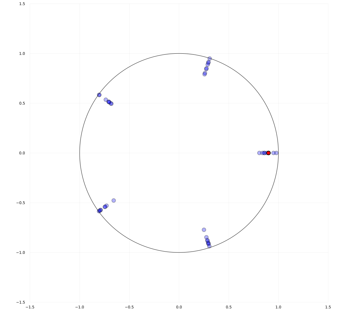
Figure 3: An example of $\mu$-nearly periodic system.

E.3 Eigenvalue estimation

We used the matrix $M$ given by

$$M:=\left(\begin{array}[]{ccccc}0&0&0&1&0\\ 0&1&0&0&0\\ 1&0&0&0&0\\ 0&0&1&0&0\\ 0&0&0&0&0.7\\ \end{array}\right).$$ (E.6)

The first $4\times 4$ block matrix is for permutation. After $N$ steps, it is expected that the last dimension shrinks so that the system becomes nearly periodic. It follows that $4!=24$ is a multiple of the length $L$. Eigenvalues of $M^{5}$ are given by $1.000,~{}1.000,~{}-0.500-0.866i,~{}-0.500+0.866i,~{}0.168$, and the $(\theta_{0},1,5)$-distinct eigenvalues are $1.000,~{}-0.500-0.866i,~{}-0.500+0.866i$.

The hyperparameters of the environment and the algorithm are summarized in Table 4. Note we don’t necessarily need $\kappa$, $B$, and $\Delta$ to run the algorithm as long as the effective sample size is sufficiently large; we used the values (satisfying the conditions) in Table 4 for simplicity.

Table 4: Hyperparameters used for eigenvalue estimation.

Hyperparameter	Value	Hyperparameter	Value
$\kappa$	$6$	a nearly period $L$	$24$
$\Delta$	$0.1$	failure probability bound $\delta$	$0.2$
dimension	$5$	observation noise proxy $R$	$0.3$
ball radius	$1$

References

- Abbasi-Yadkori et al. [2011] Y. Abbasi-Yadkori, D. Pál, and C. Szepesvári. Improved algorithms for linear stochastic bandits. Advances in neural information processing systems, 24, 2011.
- Abe and Long [1999] N. Abe and P. M. Long. Associative reinforcement learning using linear probabilistic concepts. In ICML, pages 3–11, 1999.
- Adams et al. [2021] J. Adams, N. Hansen, and K. Zhang. Identification of partially observed linear causal models: Graphical conditions for the non-Gaussian and heterogeneous cases. Advances in Neural Information Processing Systems, 34, 2021.
- Anscombe [1963] F. J. Anscombe. Sequential medical trials. Journal of the American Statistical Association, 58(302):365–383, 1963.
- Arnold [1998] L. Arnold. Random dynamical systems. Springer-Verlag, 1998.
- Auer [2003] P. Auer. Using confidence bounds for exploitation-exploration trade-offs. Journal of Machine Learning Research, 3:397–422, 2003.
- Auer et al. [2019] P. Auer, Y. Chen, P. Gajane, C. Lee, H. Luo, R. Ortner, and C. Wei. Achieving optimal dynamic regret for non-stationary bandits without prior information. In Conference on Learning Theory, pages 159–163. PMLR, 2019.
- Bennett and Kallus [2021] A. Bennett and N. Kallus. Proximal reinforcement learning: Efficient off-policy evaluation in partially observed Markov decision processes. arXiv preprint arXiv:2110.15332, 2021.
- Besbes et al. [2014] O. Besbes, Y. Gur, and A. Zeevi. Stochastic multi-armed-bandit problem with non-stationary rewards. Advances in neural information processing systems, 27, 2014.
- Bezanson et al. [2017] J. Bezanson, A. Edelman, S. Karpinski, and V. B. Shah. Julia: A fresh approach to numerical computing. SIAM review, 59(1):65–98, 2017.
- Bhouri and Perdikaris [2021] M. A. Bhouri and P. Perdikaris. Gaussian processes meet NeuralODEs: A bayesian framework for learning the dynamics of partially observed systems from scarce and noisy data. arXiv preprint arXiv:2103.03385, 2021.
- Bourgain [1993] J. Bourgain. Fourier transform restriction phenomena for certain lattice subsets and applications to nonlinear evolution equations. Geometric & Functional Analysis GAFA, 3(3):209–262, 1993.
- Bubeck and Cesa-Bianchi [2012] S. Bubeck and N. Cesa-Bianchi. Regret analysis of stochastic and nonstochastic multi-armed bandit problems. arXiv preprint arXiv:1204.5721, 2012.
- Cai et al. [2021] H. Cai, Z. Cen, L. Leng, and R. Song. Periodic-GP: Learning periodic world with Gaussian process bandits. arXiv preprint arXiv:2105.14422, 2021.
- Chen et al. [2019] Y. Chen, C. Lee, H. Luo, and C. Wei. A new algorithm for non-stationary contextual bandits: Efficient, optimal and parameter-free. In Conference on Learning Theory, pages 696–726. PMLR, 2019.
- Chesneau and Bagul [2020] Christophe Chesneau and Yogesh J. Bagul. A note on some new bounds for trigonometric functions using infinite products. Malaysian Journal of Mathematical Sciences, 14:273–283, 07 2020.
- Cheung et al. [2022] W. Cheung, D. Simchi-Levi, and R. Zhu. Hedging the drift: Learning to optimize under nonstationarity. Management Science, 68(3):1696–1713, 2022.
- Conway et al. [1970] John Conway et al. The game of life. Scientific American, 223(4):4, 1970.
- Curi et al. [2020] S. Curi, F. Berkenkamp, and A. Krause. Efficient model-based reinforcement learning through optimistic policy search and planning. Advances in Neural Information Processing Systems, 33:14156–14170, 2020.
- Dani et al. [2008] V. Dani, T. P. Hayes, and S. M. Kakade. Stochastic linear optimization under bandit feedback. pages 355–366, 2008.
- Hazan [2016] E. Hazan. Introduction to online convex optimization. Foundations and Trends® in Optimization, 2(3-4):157–325, 2016.
- Kakade et al. [2020] S. Kakade, A. Krishnamurthy, K. Lowrey, M. Ohnishi, and W. Sun. Information theoretic regret bounds for online nonlinear control. Advances in Neural Information Processing Systems, 33:15312–15325, 2020.
- Lale et al. [2020] S. Lale, K. Azizzadenesheli, B. Hassibi, and A. Anandkumar. Logarithmic regret bound in partially observable linear dynamical systems. Advances in Neural Information Processing Systems, 33:20876–20888, 2020.
- Lattimore and Szepesvári [2020] T. Lattimore and C. Szepesvári. Bandit algorithms. Cambridge University Press, 2020.
- Lee et al. [2020] A. X. Lee, A. Nagabandi, P. Abbeel, and S. Levine. Stochastic latent actor-critic: Deep reinforcement learning with a latent variable model. Advances in Neural Information Processing Systems, 33:741–752, 2020.
- Lee [2022] H. Lee. Improved rates for prediction and identification of partially observed linear dynamical systems. In International Conference on Algorithmic Learning Theory, pages 668–698. PMLR, 2022.
- Ljung [2010] L. Ljung. Perspectives on system identification. Annual Reviews in Control, 34(1):1–12, 2010.
- Luo et al. [2018] H. Luo, C. Wei, A. Agarwal, and J. Langford. Efficient contextual bandits in non-stationary worlds. In Conference on Learning Theory, pages 1739–1776. PMLR, 2018.
- Mania et al. [2020] H. Mania, M. I. Jordan, and B. Recht. Active learning for nonlinear system identification with guarantees. arXiv preprint arXiv:2006.10277, 2020.
- Menda et al. [2020] K. Menda, J. De B., J. Gupta, I. Kroo, M. Kochenderfer, and Z. Manchester. Scalable identification of partially observed systems with certainty-equivalent EM. In ICML, pages 6830–6840, 2020.
- Meng and Zheng [2010] L. Meng and B. Zheng. The optimal perturbation bounds of the Moore-Penrose inverse under the Frobenius norm. Linear algebra and its applications, 432(4):956–963, 2010.
- Mhammedi et al. [2020] Z. Mhammedi, D. J. Foster, M. Simchowitz, D. Misra, W. Sun, A. Krishnamurthy, A. Rakhlin, and J. Langford. Learning the linear quadratic regulator from nonlinear observations. Advances in Neural Information Processing Systems, 33:14532–14543, 2020.
- Moore et al. [2014] A. Moore, T. Zielinski, and A. J. Millar. Online period estimation and determination of rhythmicity in circadian data, using the BioDare data infrastructure. In Plant Circadian Networks, pages 13–44. Springer, 2014.
- Oh et al. [2019] S. Oh, A. M. Appavoo, and S. Gilbert. Periodic bandits and wireless network selection. arXiv preprint arXiv:1904.12355, 2019.
- [35] T. Oh. Note on a lower bound of the Weyl sum in Bourgain’s NLS paper (GAFA’93).
- Ohnishi et al. [2021] M. Ohnishi, I. Ishikawa, K. Lowrey, M. Ikeda, S. Kakade, and Y. Kawahara. Koopman spectrum nonlinear regulator and provably efficient online learning. arXiv preprint arXiv:2106.15775, 2021.
- Ouala et al. [2020] S. Ouala, D. Nguyen, L. Drumetz, B. Chapron, A. Pascual, F. Collard, L. Gaultier, and R. Fablet. Learning latent dynamics for partially observed chaotic systems. Chaos: An Interdisciplinary Journal of Nonlinear Science, 30, 2020.
- Robbins [1952] H. Robbins. Some aspects of the sequential design of experiments. Bulletin of the American Mathematical Society, 58(5):527–535, 1952.
- Russac et al. [2019] Y. Russac, C. Vernade, and O. Cappé. Weighted linear bandits for non-stationary environments. Advances in Neural Information Processing Systems, 32, 2019.
- Serre [1977] J.-P. Serre. Linear Representations of Finite Groups. Springer New York, NY, 1977. doi: https://doi.org/10.1007/978-1-4684-9458-7.
- Shalev-Shwartz and Ben-David [2014] S. Shalev-Shwartz and S. Ben-David. Understanding machine learning: From theory to algorithms. Cambridge university press, 2014.
- Simchowitz and Foster [2020] M. Simchowitz and D. Foster. Naive exploration is optimal for online LQR. In ICML, pages 8937–8948. PMLR, 2020.
- Song [2002] Y. Song. A note on the variation of the spectrum of an arbitrary matrix. Linear algebra and its applications, 342(1-3):41–46, 2002.
- Subramanian et al. [2022] J. Subramanian, A. Sinha, R. Seraj, and A. Mahajan. Approximate information state for approximate planning and reinforcement learning in partially observed systems. Journal of Machine Learning Research, 23(12):1–83, 2022.
- Summers et al. [2020] C. Summers, K. Lowrey, A. Rajeswaran, S. Srinivasa, and E. Todorov. Lyceum: An efficient and scalable ecosystem for robot learning. In Learning for Dynamics and Control, pages 793–803. PMLR, 2020.
- Takens [1981] F. Takens. Detecting strange attractors in turbulence. In Dynamical systems and turbulence, pages 366–381. Springer, 1981.
- Tenneti and Vaidyanathan [2015] S. V. Tenneti and P. Vaidyanathan. Nested periodic matrices and dictionaries: New signal representations for period estimation. IEEE Transactions on Signal Processing, 63(14):3736–3750, 2015.
- Trovo et al. [2020] F. Trovo, S. Paladino, M. Restelli, and N. Gatti. Sliding-window Thompson sampling for non-stationary settings. Journal of Artificial Intelligence Research, 68:311–364, 2020.
- Tsiamis and Pappas [2019] A. Tsiamis and G. J. Pappas. Finite sample analysis of stochastic system identification. In IEEE CDC, pages 3648–3654, 2019.
- Tsiamis et al. [2020] A. Tsiamis, N. Matni, and G. Pappas. Sample complexity of Kalman filtering for unknown systems. In Learning for Dynamics and Control, pages 435–444. PMLR, 2020.
- Uy and Peherstorfer [2021] W. I. T. Uy and B. Peherstorfer. Operator inference of non-Markovian terms for learning reduced models from partially observed state trajectories. Journal of Scientific Computing, 88(3):1–31, 2021.
- Von Neumann et al. [1966] J. Von Neumann, A. W. Burks, et al. Theory of self-reproducing automata. IEEE Transactions on Neural Networks, 5(1):3–14, 1966.
- Wedin [1973] P. Wedin. Perturbation theory for pseudo-inverses. BIT Numerical Mathematics, 13(2):217–232, 1973.
- Weyl [1916] H. Weyl. Über die gleichverteilung von zahlen mod eins. Math. Ann., 77:31–352, 1916.
- Wu et al. [2018] Q. Wu, N. Iyer, and H. Wang. Learning contextual bandits in a non-stationary environment. In The 41st International ACM SIGIR Conference on Research & Development in Information Retrieval, pages 495–504, 2018.