Self-Consistency of the Fokker-Planck Equation

Abstract

The Fokker-Planck equation (FPE) is the partial differential equation that governs the density evolution of the Itô process and is of great importance to the literature of statistical physics and machine learning. The FPE can be regarded as a continuity equation where the change of the density is completely determined by a time varying velocity field. Importantly, this velocity field also depends on the current density function. As a result, the ground-truth velocity field can be shown to be the solution of a fixed-point equation, a property that we call self-consistency. In this paper, we exploit this concept to design a potential function of the hypothesis velocity fields, and prove that, if such a function diminishes to zero during the training procedure, the trajectory of the densities generated by the hypothesis velocity fields converges to the solution of the FPE in the Wasserstein-2 sense. The proposed potential function is amenable to neural-network based parameterization as the stochastic gradient with respect to the parameter can be efficiently computed. Once a parameterized model, such as Neural Ordinary Differential Equation is trained, we can generate the entire trajectory to the FPE.

1 Introduction

We consider the Fokker-Planck equation (FPE) that corresponds to the Itô process with a constant diffusion coefficient, which can be written as

$$\frac{\partial}{\partial t}\alpha(t,x)+\mathrm{div}\Big{(}\alpha(t,x)(\underbrace{-\nabla V(t,x)-\nabla\log\alpha(t,x)}_{\text{underlyingvelocityfield}f^{*}(t,x)})\Big{)}=0,$$ (1)

subject to the initial condition

$$\alpha(0,x)=\alpha_{0}(x).$$ (2)

Here, $\alpha:[0,T]\times\mathcal{X}\rightarrow\mathbb{R}$ is a time varying density function defined on $\mathcal{X}\subseteq\mathbb{R}^{d}$, $V:[0,T]\times\mathcal{X}\rightarrow\mathbb{R}$ is a known potential function that determines the drifting term; $\mathrm{div}$ and $\nabla$ denote the divergence and gradient operator with respect to the spatial variable $x$ respectively. The boundary condition that we impose will be introduced in section 2.

FPE is a fundamental problem in the literature of statistical physics due to its wide applications in thermodynamic system analysis (markowich2000trend; lucia2015fokker; qi2016low) and is one of the key equations in the research of the mean field game (cardaliaguet2020introduction; gomes2014mean). Recently, it has also been used to model the dynamics of the stochastic gradient descent method on neural networks (chizat2018global; sonoda2019transport; sirignano2020mean; fang2021modeling) and the dynamics of the Rényi differential privacy (chourasia2021differential), and has become a fundamental tool for learning complex distributions and deep generative models due to its deep connection to the Wasserstein gradient flow (sohl2015deep; hashimoto2016learning; liu2019understanding; song2020score; solin2021scalable; mokrov2021large). There is a plethora of previous works trying to solve FPE numerically, including the classic mesh-based finite difference and finite volume methods (carrillo2015finite; bailo2018fully), the stochastic particle methods that are based on the discretization of the Ito SDE (dalalyan2017theoretical; li2019stochastic; li2021sqrt), the deterministic particle methods that utilize the Gaussian mollifier to approximate the dynamic (degond1990deterministic), the variational methods that are built on the Wasserstein gradient flow interpretation of the FPE (bernton2018langevin; liu2020neural; carrillo2021primal; ambrosio2005gradient; jko), and most recently the physics-informed neural network approach that directly parameterize the solution to the FPE and cast the FPE as a root finding problem (han2018solving; long2018pde; long2019pde; raissi2019physics; blechschmidt2021three). We note that in all previous approaches, the entity under consideration, i.e. the function to be approximated or learned, is explicitly the solution to the PDE eqn_FPE, which is a time-varying probability density function.

In this work, we take a different route: Instead of approximating the solution to the FPE, we propose to learn the underlying velocity field that drives the evolution of the FPE. The solution to the FPE can then be implicitly recovered by the learned velocity field. Our work is built on a concept called the self-consistency of the Fokker-Planck equation: A velocity field that correctly recovers the solution to the FPE should be a fixed point to a velocity-consistency transformation (defined in Eq. eqn_transform_A) derived from the FPE. The main contribution of our work is summarized as follows.

We establish the theoretical foundation of learning the underlying velocity field of the FPE. Specifically, we design a potential function $R$ for the hypothesis velocity fields $\{f_{n}\}$ that describes the self-consistency of the Fokker-Planck equation and show that if $R(f_{n})\rightarrow 0$ as $n\rightarrow\infty$, the trajectory of distributions generated by $f_{\infty}$ recovers the solution to the FPE in the Wasserstein-2 sense.

Moreover, when the hypothesis velocity field is parameterized as a Neural Ordinary Differential Equation $f_{\theta}$ (chen2018neural), we discuss how the stochastic gradient of the proposed potential function $R(f_{\theta})$ with respect to the parameter $\theta$ of the neural network can be efficiently computed. Therefore, once $f_{\theta}$ is trained via stochastic optimization methods, our approach returns an approximate solution to the FPE, which is non-negative and has unit mass, i.e. it integrates to $1$ on $\mathcal{X}$. These fundamental properties are crucial in real-world physics models and are not guaranteed in previous neural network based approaches.

2 Preliminaries

Boundary Condition

We assume that the process takes place on a $d$-dimensional box centered around the origin, i.e. $\mathcal{X}=[-\frac{l}{2},\frac{l}{2}]^{d}$. We consider the periodic boundary condition:

$$\alpha\left(t,(\cdots,-\frac{l}{2},\cdots)\right)= \ \alpha\left(t,(\cdots,\frac{l}{2},\cdots)\right)$$ (3)

$$\frac{\partial}{\partial x}\alpha\left(t,(\cdots,-\frac{l}{2},\cdots)\right)= \ \frac{\partial}{\partial x}\alpha\left(t,(\cdots,\frac{l}{2},\cdots)\right).$$ (4)

The above condition is the same as identifying the points on the corresponding boundaries which happens when the spatial domain is a torus. Note that on a torus, the particle that leaves the torus on the boundary will reenter the domain $\mathcal{X}$ through the boundary such that $l/2$ (resp., $-l/2$) is replaced by $-l/2$ (resp., $l/2$) in the same coordinate.

The periodic boundary condition (torus) is commonly used in the PDE analysis (e.g. see (JABIN20163588)) with an important technical merit that the integration of a periodic function on the boundary is naturally zero and hence the analysis using integration by parts can be simplified. Moreover, it also allows us to focus on the behavior of the PDE system on compact domains without sacrificing the generality, since we can always set the diameter of the torus to be sufficiently large. We emphasize that to the ML community, this is usually the case of interest: Only in a bounded domain can we expect a neural ODE to be able to represent the underlying velocity field of the FPE, since the neural network is not a universal function approximator on unbounded domains.

In the following, we refer to periodic functions with a period of $l$ as $l$-periodic.

Velocity Field and the Induced Push-forward Map

A velocity field is map $f:[0,T]\times\mathcal{X}\rightarrow\mathbb{R}^{d}$ that determines the movement of a particle $x(t)$:

$$\frac{\mathrm{d}}{\mathrm{d}t}x(t)=f(t,x(t))$$ (5)

A velocity field $f(t,x)$ induces a push-forward map $X(t,x;f)$ via integrating over time

$$X(t,x_{0};f)=x_{0}+\int_{0}^{t}f(s,x_{s})\mathrm{d}s,$$ (6)

where $\{x_{s}\}_{s=0}^{t}$ is the trajectory of a particle following the velocity field $f(t,x)$ with the initial position $x_{0}$. Note that the map $X(t,x;f)$ is invertible under the assumption that $f(t,x)$ is Lipschitz continuous in $x$ for all $t$. Additionally $X(t,x;f)-x$ is $l$-periodic if we further assume that $f$ is $l$-periodic: For any $i\in\{1,\ldots,d\}$

$$X(t,x_{0}+le_{i};f)-(x_{0}+le_{i})=\int_{0}^{t}f(s,x_{s}+le_{i})\mathrm{d}s=\int_{0}^{t}f(s,x_{s})\mathrm{d}s=X(t,x_{0};f)-x_{0}.$$ (7)

When the velocity $f$ is clear from the context, we omit the dependence of $X$ on $f$ and write $X(t,x)$, for simplicity.

Neural Ordinary Differential Equation

The neural ordinary differential equation (NODE) is a favorable instance of the hypothesis class since neural networks are universal function approximators in a bounded domain and have achieved great recent success in machine learning (chen2018neural; dupont2019augmented; choromanski2020ode). Let $f:\mathbb{R}\times\mathbb{R}^{d}\times\Theta\rightarrow\mathbb{R}^{d}$ be a neural network parameterized by $\theta\in\Theta$. A $d$-dimensional NODE in can be described as

$$\frac{\mathrm{d}}{\mathrm{d}t}x(t)=f_{\theta}(t,x(t)).$$ (8)

To accommodate the periodic boundary conditions eqn_bc_0 and eqn_bc_1, we need the NODE to be $l$-periodic. Consider a $2d$-dimensional NODE with velocity $\tilde{f}$. We can construct a $d$-dimensional NODE with the following hypothesis velocity field

$$f_{\theta}(t,x(t))=\tilde{f}_{\theta}\left(t,\pmatrix{\sin}\frac{2\pi}{l}x(t)\\ \cos\frac{2\pi}{l}x(t)\right).$$ (9)

Here $\sin$ and $\cos$ are applied in an element-wise manner.

Notations

Consider the $d$-dimensional index vector $a=(a_{1},\ldots,a_{d})$ with $a_{i}\in\mathbb{N}$ and $\|a\|_{1}=k$ and a map $f:\mathbb{R}^{d}\rightarrow\mathbb{R}^{d}$. Denote

$$f^{(a)}=\left[\frac{\partial^{k}f_{1}}{\partial x_{1}^{a_{1}}\ldots\partial x_{d}^{a_{d}}},\cdots,\frac{\partial^{k}f_{d}}{\partial x_{1}^{a_{1}}\ldots\partial x_{d}^{a_{d}}}\right],$$ (10)

where $f_{i}$ denotes the $i$th entry of $f$. We define the $k$th order Sobolev norm of a map $f:\mathcal{X}\rightarrow\mathbb{R}^{d}$ with a base measure $\mu\in\mathcal{M}_{+}^{1}(\mathcal{X})$ by

$$\|f\|_{W^{k,2}(\mu)}=\left(\sum_{i=0}^{k}\int_{\mathcal{X}}\|f^{(i)}(x)\|^{2}\mu(x)\mathrm{d}x\right)^{\frac{1}{2}}.$$ (11)

Here $f^{(k)}=\{f^{(a)}\}_{a:\|a\|_{1}=k}$ denotes the collection of all $k$th order partial derivatives of the map $f$ and is regarded as a $d^{k+1}$-dimensional vector. We use $\|\cdot\|$ to denote the spectral norm for matrices and tensors and the standard $\ell_{2}$-norm for vectors.
We use $\{e_{i}\}$ to denote the standard basis of $\mathbb{R}^{d}$ and use $\Delta$ to denote the Laplacian operator on the spatial variable. We use $\nabla^{i},i\geq 2$ to denote higher order gradient.

3 Methodology

Recall that on a torus, when a particle leaves the domain on a boundary, it reappears on the other side (see Figure 1-(a)). Therefore, the velocity field of the particles are discontinuous on the boundaries, which introduces difficulties in function approximation. To avoid this issue, a useful and equivalent perspective of the periodic boundary condition is to think of the density function $\alpha(t,\cdot)$ as a $l$-periodic function in every coordinate, i.e.

$$\forall t,x,\quad\alpha(t,x+le_{i})=\alpha(t,x),i\in[d],$$ (12)

which is depicted in (b) of Figure 1. While particles are allowed to leave $\mathcal{X}$, the domain of interest, due to the periodicity of the whole domain $\mathbb{R}^{d}$, the total mass within $\mathcal{X}$ is conserved since the influx and the outflow are balanced.

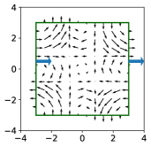
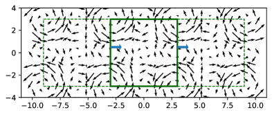
(a)	(b)

Figure 1: Figure (a) depicts that when a particle leaves the torus on a boundary, it reappears on the other side. The velocity field is discontinuous on the boundary. In Figure (b), we consider the periodic extension of the density function $\alpha(t,x)$. This is equivalent to the torus since whenever a particle leaves the boundary, another particle will enter $\mathcal{X}$ from a corresponding adjoining cell. Note that in Figure (b) the velocity field is continuous on the whole domain.

3.1 Self-consistency of the Fokker-Planck Equation

Suppose that the particles are distributed initially according to the distribution $\alpha_{0}$ defined in eqn_FPE_initial and follow a hypothesis velocity field $f(t,x)$. From this perspective, we can write the distribution of particles on $\mathcal{X}$ at time $t$ in a push-forward manner

$$\rho^{1}(t,\cdot;f)=X(t,\cdot;f)\sharp\alpha_{0},$$ (13)

where the push-forward map $X$, induced by the velocity $f$, is defined in eqn_push_forward_map. Note that $\rho^{1}$ is well-defined on the whole domain $\mathbb{R}^{d}$, but we restrict our interest to $\mathcal{X}$. Based on this notation, the Fokker-Planck equation eqn_FPE induces a velocity-consistency transformation $\mathcal{A}$ of the velocity field in the following manner:

$$\mathcal{A}[f](t,x)=-\nabla V(t,x)-\nabla\log\rho^{1}(t,x;f).$$ (14)

Observe that, for the ground-truth velocity field $f^{*}$ that drives the particle evolution of the Fokker-Planck equation, i.e. $f^{*}(t,x)=-\nabla V(t,x)-\nabla\log\alpha(t,x)$, we have

$$\mathcal{A}[f^{*}]=f^{*}.$$

We term this property the self-consistency of the Fokker-Planck equation. Similar to Eq. eqn_pushforward_rho1, we can define $\rho^{2}(t,\cdot;f)=X(t,\cdot;\mathcal{A}[f])\sharp\alpha_{0},$. Indeed, the interplay between the two systems $\rho^{1}$ and $\rho^{2}$ is crucial to our analysis.

The goal of our paper is to show that if a sequence of hypothesis velocity fields $\{f_{n}\}$ asymptotically satisfies the above consistency property, i.e. $\|\mathcal{A}[f_{n}]-f_{n}\|\rightarrow 0$ as $n\rightarrow\infty$ for some appropriate norm $\|\cdot\|$, then the distribution $\rho^{1}(t,x;f_{\infty})$ generated from the hypothesis velocity field $f_{\infty}$ recovers $\alpha(t,x)$, the solution to the FPE eqn_FPE in the Wasserstein-2 sense.

3.2 Designing the Self-Consistency Potential Function and its Computation

Given a hypothesis velocity field $f$, we denote the difference between $f$ and $\mathcal{A}[f]$ by

$$\delta(t,x;f)=f(t,x)-\mathcal{A}[f](t,x).$$ (15)

We propose to use the time average of the $2$nd order Sobolev norm of $\delta$ with the base measure $\rho^{1}(t,\cdot;f)$ as the potential function of $f$: