Optimized Quantum Phase Estimation for Simulating Electronic States in Various Energy Regimes.

Abstract

While quantum algorithms for simulation exhibit better asymptotic scaling than their classical counterparts, they currently cannot be implemented on real-world devices. Instead, chemists and computer scientists rely on costly classical simulations of these quantum algorithms. In particular, the quantum phase estimation (QPE) algorithm is among several approaches that have attracted much attention in recent years for its genuine quantum character. However, it is memory-intensive to simulate and intractable for moderate system sizes. This paper discusses the performance and applicability of QPESIM, a new simulation of the QPE algorithm designed to take advantage of modest computational resources. In particular, we demonstrate the versatility of QPESIM in simulating various electronic states by examining the ground and core-level states of H₂O. For these states, we also discuss the effect of the active-space size on the quality of the calculated energies. For the high-energy core-level states, we demonstrate that new QPE simulations for active spaces defined by 15 active orbitals significantly reduce the errors in core-level excitation energies compared to earlier QPE simulations using smaller active spaces.

I Introduction

The emergence of quantum computing technologies promises to provide new modeling tools that eliminate known deficiencies of many-body formulations designed to take advantage of classical computing. Among these, one can highlight the exponential growth in the computational demands for methods that provide the so-called full configuration interaction (FCI) level of accuracy, which is needed to provide the quantitatively correct level of accuracies required in predictive computational chemistry. Another well-known deficiency is an inherent bias (biases), or limited applicability, of all approximations used in quantum chemistry. For example, in the area of wave function based correlated methods, the applicability of single-reference many-body perturbation theory (MBPT) or single-reference coupled-cluster (CC) methods Coester (1958); Coester and Kummel (1960); Čížek (1966); Paldus et al. (1972); Purvis and Bartlett (1982); Koch and Jørgensen (1990); Paldus and Li (1999); Crawford and Schaefer (2000); Bartlett and Musiał (2007) is limited by the quality of the so-called reference function, i.e., a Slater determinant that provides a zeroth-order approximation to the exact ground-state wave function. A typical way of manifesting these problems is associated with the nonuniform level of accuracy of calculated energies on the ground-state potential energy surfaces. For example, while MBPT methods provide a reasonable level of accuracy for the regions close to the equilibrium geometry of a given molecular system, the same techniques fail for stretched bond distances. Similarly, the applicability of multi-reference CC or CI methods Mukherjee et al. (1975); Kutzelnigg (1982); Stolarczyk and Monkhorst (1985); Jeziorski and Paldus (1989); Rittby and Bartlett (1991); Kaldor (1991); Meissner (1998); Jeziorski and Monkhorst (1981); Meissner et al. (1988); Pittner et al. (1999); Mahapatra et al. (1998, 1998); Evangelista et al. (2007); Lyakh et al. (2012) is limited by the quality of model/active spaces that cannot be universally defined for all geometries involved in studies of chemical transformations usually related to bond-forming and bond-breaking processes. On the other hand, quantum algorithms are capable of alleviating issues with identifying electronic states of interest. An excellent illustration of this is the quantum phase estimation (QPE) methodKitaev (1997); Nielsen and Chuang (2011); Luis and Peřina (1996); Cleve et al. (1998); Berry et al. (2007); Childs (2010); Seeley et al. (2012); Wecker et al. (2015); Häner et al. (2016); Poulin et al. (2017); Berry et al. (2006). The probability of detecting a phase of a particular electronic state is proportional to the square of the overlap between the initial state used as a starting point for the unitary time evolution and exact wave function. Therefore, one can use the trial wave function as a form of the hypothesis to get the statistical echo of relevant exact states (and corresponding phases) that have a non-zero overlap with the trial wave function. Recently, we have tested these algorithms on the example of valence excited states and high-energy states corresponding to excitations of electrons occupying inner atomic shells. When fault-tolerant quantum platforms are available, the QPE algorithms should be advantageous to the existing approximations for simulating core-level states on conventional computer platforms, especially in the context of identifying complex excited states dominated by multi-electron excitations. In studies of excited-state processes, the QPE approach has a clear advantage over the other algorithms, such as the Variational Quantum Eigensolver (VQE), Peruzzo et al. (2014); McClean et al. (2016); Romero et al. (2018); Shen et al. (2017); Kandala et al. (2017, 2019); Colless et al. (2018); Huggins et al. (2020); Cao et al. (2019); Anand et al. (2021) designed to utilize noisy intermediate-scale quantum (NISQ) devices, because detailed knowledge of the sought-after state is not required before the simulation.

The main focus of this paper is to highlight a recently developed QPE simulator that allows for scalable simulations of previously inaccessible atomic and molecular systems. We will discuss the implementation details, which allow us to execute sizable QPE simulations for systems described by 10-20 molecular orbitals using modest computational resources provided by broadly accessible commodity computer systems. We will also illustrate the importance of this expanded QPE capability by studying the behavior of the ground and core-level energies as functions of the active-space size. As a benchmark system, we chose to investigate the ground and core-level excited states of H₂O.

The paper is organized as follows: in Section 1, we provide an overview of the QPE algorithm. In Sections 2 and 3, we provide implementation details and a short description of the interface between the QPE algorithm and the NWChem Valiev et al. (2010); Apra et al. (2020) suite of computational chemistry software, which provides one- and two-electron integrals files and the second quantized characterization of the trial wave function, respectively. In Section 4, we discuss the results of the quantum algorithm simulations of H₂O, with special attention paid to the simulations of core-level excitations in the water molecule employing large active spaces. We demonstrate that using fifteen-orbital active space leads to a three-fold reduction of error in calculated core-level excitation energy discussed in Ref. (47). This result provides a strong argument for developing QPE algorithms for various types of x-ray spectroscopies and, in a more general perspective, identifying electronic states in arbitrary energy regimes.

II Methodology

The main goal of quantum chemistry is to find high-quality approximate form of solution to the electronic Schrödinger equation

$$H|\Psi_{K}\rangle=E_{K}|\Psi_{K}\rangle\;,$$ (1)

where the electronic Hamiltonian $H$ depends parametrically on the coordinates of nuclei that form a fixed nuclear frame and $E_{K}$ and $|\Psi_{K}\rangle$ correspond to energy and wave function corresponding to $K$-th electronic state. The simulations of excited states usually involve a specific form of the excited-state wave function ansatz. For example, in the ubiquitous equation-of-motion coupled-cluster formalism (EOMCC), Geertsen et al. (1989); Comeau and Bartlett (1993); Stanton and Bartlett (1993) the $K$-state is parametrized using the following Ansatz

$$|\Psi_{K}\rangle=R_{K}e^{T}|\Phi\rangle\;,$$ (2)

where $R_{K}$ and $T$ are many-body cluster and excitation operators and $|\Phi\rangle$ is the so-called reference function. To obtain accurate estimates of excitation energies for complex excited states, one needs to include high-rank collective excitations, which in many cases leads to insurmountable computational bottlenecks. Quantum computing and QPE formalism, in particular, have the potential to bypass these problems.

The language of second-quantization is not only a convenient language to express electronic Hamiltonian

$$H=\sum_{p,q}h_{pq}a^{\dagger}_{p}a_{q}+\frac{1}{2}\sum_{p,q,r,s}h_{pqrs}a^{\dagger}_{p}a^{\dagger}_{q}a_{r}a_{s}$$ (3)

and assure the anti-symmetry of the corresponding wave functions, but also gives rise to an efficient diagrammatic techniques for book-keeping the electron correlation effects of various order. The multi-dimensional tensors $h_{pq}$ and $h_{pqrs}$ are referred to as the one- and two-electron integrals. In Eq. (3), the creation/annihilation operators $a_{p}^{\dagger}$/$a_{p}$ for electrons in $p$-th single particle state (spin orbital) satisfy the standard Fermionic anti-commutation relations

$$[a_{p},a_{q}]_{+}=[a_{p}^{\dagger},a_{q}^{\dagger}]=0\;,$$ (4)

$$[a_{p},a_{q}^{\dagger}]_{+}=\delta_{pq}\;,$$ (5)

where $[A,B]_{+}=AB+BA$. Various spin orbitals bases can be used to express second quantized operators. In this paper, we will focus on the restricted Hartree-Fock (RHF) in calculations for ground and core-level states, and second-order MBPT natural orbitals (nMP2) in calculations for ground state energies. Assuming that we are dealing with system with $k_{\alpha}$ and $k_{\beta}$ $\alpha$ and $\beta$ electrons occupying $n$ orbitals, which corresponds to the wave function with defined $S_{z}$ quantum number, then the number of determinants in the FCI problem, $N_{\rm det}^{\rm(FCI)}$, corresponding to (1) is equal to

$$N_{\rm det}^{\rm(FCI)}={n\choose k_{\alpha}}{n\choose k_{\beta}}\;.$$ (6)

This dimensionality can be further reduced by incorporating spin and spatial symmetry of the system of interest. However, for realistic systems, this leads to prohibitive costs for simulation on classical computers.

II.1 Review of Hamiltonian Simulation via Quantum Phase Estimation

As broadly discussed in the literature, quantum algorithms that simulate the quantum evolution of a system described by Hamiltonian $H$ have asymptotically superior performance over classical ab initio techniques, enabling polynomial time and space complexity simulations. One technique, phase estimation-based Hamiltonian simulation, requires only a linear number of qubits relative to the number of orbitals Whitfield et al. (2011). We focus on phase estimation for its simplicity and utility.

In this section, we first describe the phase estimation-based Hamiltonian simulation, including how Hamiltonians can be efficiently mapped to quantum architectures via the Jordan–Wigner transformation. Then, we discuss the role of the Lie–Trotter–Suzuki product formulas and error scaling. Finally, we describe how phase estimation can be used to extract the energy eigenvalue.

II.1.1 Jordan–Wigner Transformation

There are several transformations to map electronic Hamiltonians onto a register of qubits, including the Jordan–Wigner and Bravyi–Kitaev transformations Whitfield et al. (2011); Seeley et al. (2012). Among them, the simplest (and historically oldest) is the Jordan–Wigner (JW) transformation that enables the representation of fermionic operators in terms of quantum gates:

$$a^{\dagger}_{l}=\bigotimes_{k=1}^{l-1}Z_{k}\frac{X_{l}-iY_{l}}{2}\qquad a_{l}=\bigotimes_{k=1}^{l-1}Z_{k}\frac{X_{l}+iY_{l}}{2}\;,$$ (7)

where $X,Y,Z$ are Pauli operators. Although the JW transformation is a non-local mapping in terms of fermionic degrees of freedom, it is sufficiently efficient in medium-scale applications to demonstrate the basic features of discussed quantum algorithms. The JW mapping transforms the second quantized Hamiltonian (3) into a linear combination of unitaries (or Pauli strings) $P_{k}$

$$H_{JW}=\sum_{k=1}^{m}H_{k}=\sum_{k=1}^{m}h_{k}P_{k}\;,$$ (8)

where $h_{k}$ is a scalar factor. In our simulated systems, we assume that $h_{k}\in\mathbb{R}$, though there exist systems where $h_{k}\in\mathbb{C}$.

II.1.2 Trotterization

Because $H_{JW}$ is Hermitian, $e^{-iH_{JW}t}$ is unitary and thus implementable on a quantum computer Whitfield et al. (2011). This operator can then be decomposed into a series of implementable unitaries on a quantum device via the Lie–Trotter–Suzuki matrix product formula Hatano and Suzuki (2005). In particular, when $t\ll 1$, the first order non-symmetric Trotter formula can be applied as follows:

$$\left\lVert e^{-iH_{JW}t}-\prod_{k=1}^{m}e^{-iH_{k}t}\right\rVert\in\mathcal{O}(m^{2}t^{2})\;,$$ (9)

where $e^{-iH_{k}t}$ is implementable (the precise circuits required are further described in Ref. (51)). Thus, the exponentiated second-quantized Hamiltonian can be simulated on a quantum computer, with quadratic error scaling. Furthermore, this technique can be generalized when we no longer can guarantee $t\ll 1$ via Trotterization. By selecting some number of Trotter steps $r$, we approximate the timesliced evolution operator $e^{-iH_{k}t/r}$ with $e^{iH_{k}t/r}$ terms, which has error scaling in:

$$\left\lVert e^{-iH_{JW}t}-\left(\prod_{k=1}^{m}e^{-iH_{k}(t/r)}\right)^{r}\right\rVert\in\mathcal{O}\left(\frac{m^{2}t^{2}}{r}\right)\;.$$ (10)

Thus, by selecting $r$ appropriately with respect to the desired $t$ and the number of Hamiltonian terms $n$, an acceptable error bound can be derived. Furthermore, this was simply the first order, non-symmetric Trotter formula; higher-order formulas exist and have preferable asymptotic scaling at the cost of quantum operations Berry et al. (2006).

II.1.3 Quantum Phase Estimation and Scaling

Now that we can implement an approximation of $e^{-iHt}$ with constrained error, we must extract the energy eigenvalue from the operator. Recall that for any eigenvector $\left|\psi\right\rangle$ of the electronic Hamiltonian we have:

$$e^{-iHt}\left|\psi\right\rangle=e^{-iE_{\psi}t}\left|\psi\right\rangle$$ (11)

where $E_{\psi}$ is the associated energy level. Thus, the core challenge is to extract the phase $E_{\psi}$ from the coefficient. In fact, this is precisely the objective of phase-estimation (PE) techniques Svore et al. (2013). PE operates such that, given a unitary $U$, eigenvector $\left|\psi\right\rangle$, and the number of precision bits $p$, we can extract the phase $\phi$:

$$U\left|\psi\right\rangle=e^{2\pi i\phi}\left|\psi\right\rangle\;.$$ (12)

using an additional $p$ qubits for precision. Recognize that Eq. 11 is precisely the form of Eq. 12 when $2\pi\phi=-E_{\psi}t$. Thus, we can apply PE to the Hamiltonian operator $e^{-iHt}$, and compute the energy as follows:

$$E_{\psi}=\frac{2\pi}{t}\phi\;.$$ (13)

When the time evolution operator is Trotterized, it typically is applied once as opposed to $r$ times. This still allows us to extract the energy:

$$e^{-iHt/r}\left|\psi\right\rangle=e^{-iE_{\psi}t/r}\left|\psi\right\rangle\implies E_{\psi}=\frac{-2\pi r}{t}\phi\;.$$ (14)

We typically take $t=1$, so that $E_{\psi}=-(2\pi r)\phi$. Thus, given a phase estimate from PE, we can produce an estimation of the energy eigenvalue.

In our implementation, we emulate a Fourier-based quantum phase estimation (QPE) Abrams and Lloyd (1999). QPE requires $2^{p}-1$ applications of $U$, $p+2n$ qubits, where $2n$ corresponds to the number of spin orbitals, and applies the inverse quantum Fourier transform to produce $\phi$, which can be used to compute $E_{\psi}$.

III Algorithm

The discussed implementation of the QPE algorithm (QPESIM) has been developed using a C++ environment Kang et al. (2022) and is optimized to take advantage of mid-range computer architectures. QPESIM is capable of performing QPE simulations for chemical systems and processes driven by ground and/or excited states in various energy regimes. In the following section, we provide details of QPESIM’s implementation.

III.1 Psuedocode and Implementation

Our algorithm simulates QPE-based energy estimation on molecular Hamiltonians. QPESIM (Algorithm 1) takes as input Hamiltonians produced by NWChem in the Broombridge format, a starting state to simulate, and two initial hyperparameters $p$, the number of bits of precision for phase estimation, and $r$, the number of Trotter steps. The algorithm then outputs a probability distribution over all phases from $0$ to $2^{p}-1$:

Input: A second quantized Hamiltonian $H$ with $n$ orbitals and $k_{\alpha}+k_{\beta}=2k_{\alpha}$ electrons stored as an array of classes of terms, $p$ number of ancilla precision bits, $r$ steps

Output: Probabilities, a vector of length $2^{p}$ with the probability of each phase after QPE

StateVector $\leftarrow$ complex, combinatorial ansatz vector of length $\binom{n}{k_{\alpha}}\binom{n}{k_{\alpha}}2^{p}$

for $i=0$; $i\leq 2^{p}-1$; $i+=1$ do

       ApplyUnitary(i, StateVector)

      

Probabilities $\leftarrow$ InverseQuantumFourierTransform(StateVector)

return StateVector

Algorithm 1 SIMULATE emulates QPE-based Hamiltonian simulation

The key contribution is that StateVector has an improved data representation that enables a superpolynomial reduction in space complexity. In Section III.2, we discuss the data layout of StateVector. Then, in Section III.3, we describe the implementation of new loop update structures to execute ApplyUnitary on the novel data layout.

III.2 Representing Data in StateVector

One of the limiting factors for typical quantum simulators is the naïve preparation of state vectors, often ignoring the symmetries of molecular systems. QPESIM improves upon this by being mindful of the chemical problem at hand and accounting for electronic symmetries when storing configuration amplitudes in StateVector. The benefit of the state preparation in QPESIM is fully appreciated when describing the algorithm using the occupation number representation.

III.2.1 Occupation Number Representation

For interacting fermionic systems, to describe the action of the creation/annihilation operators on the Slater determinants it is convenient to invoke the occupation number representation, where each Slater determinant is represented as a vector

$$|n_{M}\;n_{M-1}\;\ldots\;n_{i+1}\;n_{i}\;n_{i-1}\;\ldots\;n_{1}\rangle$$ (15)

where occupation numbers $n_{i}$ are equal to either 1 (electron occupies $i$-th spin orbital) or 0 (no electron is occupying $i$-th spin orbital). In (15), $M$ stands for the total number of spin orbitals used to describe quantum system and $M=2n$, where $n$ is the number of orbitals.

The following formulas give the non-trivial action of creation/annihilation operators on the state vectors

$$a_{i}^{\dagger}|n_{M}\;n_{M-1}\;\ldots\;n_{i+1}\;0\;n_{i-1}\;\ldots n_{1}\;\rangle = (-1)^{\sum_{k=1}^{i-1}n_{k}}|n_{M}\;n_{M-1}\;\ldots\;n_{i+1}\;1\;n_{i-1}\;\ldots n_{1}\;\rangle\;\;\;\;\;\;$$ (16)

$$a_{i}|n_{M}\;n_{M-1}\;\ldots\;n_{i+1}\;1\;n_{i-1}\;\ldots n_{1}\;\rangle = (-1)^{\sum_{k=1}^{i-1}n_{k}}|n_{M}\;n_{M-1}\;\ldots\;n_{i+1}\;0\;n_{i-1}\;\ldots n_{1}\;\rangle.$$ (17)

It should be stressed that the language of second quantization automatically assures proper anti-symmetry of the wave function expansions.

Since the discussed implementation of the QPE algorithm utilizes the list of the configurations in the occupation number representation, it is easy to incorporate various symmetries, including spin and spatial symmetries of the quantum system of interest. Another essential element of flexibility is the possibility of restricting the configurational space for the QPE simulations. For example, one can envision the process of selecting configurations that correspond to the Hartree-Fock determinant and all singly, doubly, triply, and quadruply excited Slater determinants with respect to the HF Slater determinant. This allows one to form the analogs of the truncated or even adaptive (multi-reference and/or state-selective) configuration-interaction expansions. In the example above, the selection of amplitudes would provide CISDTQ (configuration interaction with singles, doubles, triples, and quadruples) energies in the QPE simulations.

III.2.2 QPESIM approach to state vectors

Existing quantum simulators store all potential qubit configurations: assuming $n$ is the number of orbitals, simulators must store $2^{M}=2^{2n}$ amplitudes. This is because each of the $2n$ spin orbitals are allocated a qubit in QPE, so each configuration from $00...0$ to $11...1$ must be stored. However, when accounting for symmetries and conservation of electrons, there are only at most $N_{\rm det}^{\rm(FCI)}$ valid configurations. Thus, using general-purpose quantum emulators for simulation algorithms often amounts to storing significantly more amplitudes than necessary to simulate the system.

Our algorithm exploits configuration constraints by creating a vector StateVector which only stores valid configurations. The data structure itself can be represented as a 3D array defined by three indices: $l$, $c_{1}$, and $c_{2}$. In a given layer $(l,c_{1},c_{2})$, $l$ expresses the number of times the unitary $\prod_{j=1}^{n}e^{-iH_{j}t/r}$ has been applied and $c_{1}$ and $c_{2}$ serve as indices for $\binom{n}{k_{\alpha}}$ alpha and $\binom{n}{k_{\beta}}$ beta spin-orbital configurations in the amplitude vector, respectively. In our simulated system of H₂O with 15 orbitals, this exhibits about a 100x reduction in memory, and the savings would only be greater for larger systems. In general, our approximation has a memory reduction of at least $2^{M}/N_{\rm det}^{\rm(FCI)}$ compared to traditional quantum simulation approaches.

III.3 Updating StateVector

While the StateVector format requires asymptotically less memory, it also requires a new update scheme. Matrix-based emulators simply use existing matrix product libraries to compute a series of matrix-vector products; in QPESIM, we instead iterate over the Hamiltonian terms and directly apply updates to the respective StateVector indices.

To achieve the update, we analyze the impacts of each type of Hamiltonian term on StateVector. Out of the five Hamiltonian term types, $pp$, $pq$, $pqqp$, $pqqr$, and $pqrs$, two classes can be created:

1. Configuration preserving ($pp$, $pqqp$): these terms only modify the coefficient of configurations. Thus, the $pp$/$pqqp$ terms simply apply a multiplicative scalar coefficient

2. Configuration modifying ($pq$, $pqqr$, $pqrs$): these terms represent interactions between two electronic configurations. Thus, these terms apply a 2x2 matrix transformation to an electron configuration and its conjugate.

III.3.1 Configuration Preserving Terms

We first provide the effect of the configuration preserving operators. Suppose we have operators $a_{p}^{\dagger}$, $a_{p}$ operating on the spin orbital $p$ and an arbitrary state

$$|\ldots\;n_{p}\;\ldots\rangle$$ (18)

where $p$-th spin orbital is occupied (i.e. $n_{p}=1$) then using definitions (16) and (17) the action of the $pp$ transformations ($a_{p}^{\dagger}a_{p}$) and their exponentials on the above vector is given by the formula

$$e^{-i(h_{pp}(a^{\dagger}_{p}a_{p}))t}|\ldots\;n_{p}\;\ldots\rangle=e^{-i(h_{pp}n_{p})t}|\ldots\;n_{p}\;\;\ldots\rangle\;\;(n_{p}=1)\;.$$ (19)

Similarly, if in the state

$$|\ldots\;n_{q}\;\ldots\;n_{p}\;\ldots\rangle\;,$$ (20)

spin orbitals $p$ and $q$ are occupied (i.e., $n_{p}=n_{q}=1$) then the action of the $pqqp$ transformation on this vector can be written as:

$$e^{-i(h_{pqqp}(a^{\dagger}_{p}a^{\dagger}_{q}a_{q}a_{p}))t}|\ldots\;n_{q}\;\ldots\;n_{p}\;\ldots\rangle =e^{-i(h_{pqqp}n_{p}n_{q})t}|\ldots\;n_{q}\;\ldots\;n_{p}\;\ldots\rangle\;\;(n_{p}=n_{q}=1)$$ (21)

This is a consequence of the fact that for $p\neq q$ the product $a_{p}^{\dagger}a_{q}^{\dagger}a_{q}a_{p}$ is equal to the product of particle number operators $\hat{n}_{p}\hat{n}_{q}$ where $\hat{n}_{p}=a_{p}^{\dagger}a_{p}$ and $\hat{n}_{q}=a_{q}^{\dagger}a_{q}$.

On all other states, these transformations simply apply identity. Thus, for the $pp$/$pqqp$ terms, QPESIM simply needs to find affected indices and multiply the associated coefficients by $e^{-ih_{pp}t/r},e^{-ih_{pqqp}t/r}$, respectively. In code, this is implemented as:

⬇

StateVector[psi_pp_index] *= std::exp(-i * hpp * t)

StateVector[psi_pqqp_index] *= std::exp(-i * hpqqp * t)

III.3.2 Configuration Modifying Terms

The second class of terms, $pq$, $pqqr$, and $pqrs$, require more complex updates. In contrast to the configuration preserving terms, the $pq$, $pqqr$, and $pqrs$ terms can produce singly or doubly excited configurations with respect to the configuration these terms are acting on.

By using the Jordan–Wigner transformation, we can derive an explicit form for the 2x2 linear transformation given the coefficients of the two configurations. In particular, it’s necessary to introduce $\eta$, the parity of the bits between the $p,q,r,s$ orbitals. For example, suppose $h$ is the Hamiltonian term coefficient of an $a_{p}^{\dagger}a_{q}^{\dagger}a_{s}a_{r}$ string and $\alpha_{\left|01\right\rangle}$ and $\alpha_{\left|10\right\rangle}$ are the coefficients of the conjugate configurations for that specific term. Then, the transformation can be described via a linear, symmetric matrix:

$$\begin{bmatrix}\cos(ht)&(-1)^{\eta+1}i\sin(ht)\\ (-1)^{\eta+1}i\sin(ht)&\cos(ht)\end{bmatrix}\begin{bmatrix}\alpha_{\left|01\right\rangle}\\ \alpha_{\left|10\right\rangle}\end{bmatrix}$$ (22)

This simplified translation also reduces the complexity of the code, as all terms can be reduced to accessing at most two elements of the state vector. Thus, the following code is sufficient:

⬇

void updateStateVector(std::array<std::complex<double>, 4> coeffs,

unsigned leftIdx, unsigned rightIdx)

{

stud::complex<double> left, right;

left = StateVector[leftIdx];

right = StateVector[rightIdx];

StateVector[leftIdx] = left * coeffs[0] + right * coeffs[1];

StateVector[rightIdx] = left * coeffs[1] + right * coeffs[0];

}

III.3.3 ApplyUnitary Pseudocode

In order to identify the indices to modify, we employ the following loop hierarchy in the ApplyUnitary method (Algorithm 2):

1. Class of Hamiltonian term (for each type $pp$, $pqqp$, $pq$, $pqqr$, $pqrs$, there is a list of Hamiltonian terms $H_{pp},H_{pqqp},H_{pq},H_{pqqr},H_{pqrs}$)

2. Term within the class

3. Affected amplitudes/state vector indices

This produces the following update algorithm:

Input: Sets of terms broken by class, $H_{pp},H_{pqqp},H_{pq},H_{pqqr},H_{pqrs}$ and a starting ansatz StateVector

Output: $e^{-iHt}$ is applied once to StateVector

for Class in $\{H_{pp},H_{pqqp},H_{pq},H_{pqqr},H_{pqrs}\}$ do

       for Term in Class do

             for Configuration affected by Term do

                   IndicesToUpdate $\leftarrow$ ConfigurationToIndex(Configuration)

                   UpdateStateVector(IndicesToUpdate, Term.coefficients)

                  

            

      

Algorithm 2 ApplyUnitary applies the $e^{-iHt}$ unitary once

Note that we update the state vector in a particular ordering, as specific Hamiltonian orderings affect the accuracy of the Trotter–Suzuki formulaHastings et al. (2014).

IV Results & Discussion

We chose the H₂O as an exemplary system that we could examine both ground and high-energy excited states with while going beyond the capabilities of alternative QPE solvers. The geometry of the system is given by $R_{\rm OH}=0.95778$ Å and $\theta_{HOH}=104.47984^{\circ}$. In our earlier study Bauman et al. (2020), we demonstrated the utility of the QPE algorithm in targeting core-level excited states. However, we were restricted to stinted active spaces that lead to understandably imperfect results when compared to experimental results. In this study, we employed an active space consisting of the 15 lowest-lying RHF orbitals and MP2 natural orbitals of the cc-pVDZ basis set (24 orbitals in the full basis).

Our primary contribution, a new algorithm for quantum phase estimation-based simulation, requires significantly less memory than general purpose quantum simulators and integrates with NWChem and the Broombridge Hamiltonian format. Our end-to-end pipeline, as described in Figure 1, first ingests Broombridge Hamiltonians from NWChem, converts it to a Jordan–Wigner Hamiltonian, and runs the simulation. The final output is a distribution of phases corresponding to the predicted energy level of the system.

When we view the phase distributions on our sample systems (see Figures 2-4), the phase results reflect how well our ansatz approximates the target-state eigenvector, as seen in the probability distribution of the phases. Essentially, while the Trotter formula does slightly modify the true eigenvectors, we would expect an ansatz with high overlap with the original target-state configuration to also have a phase readout with a high probability of measuring the correct energy phase. In particular, by taking the phase(s) with the highest probability, we can produce an energy level estimate of the system.

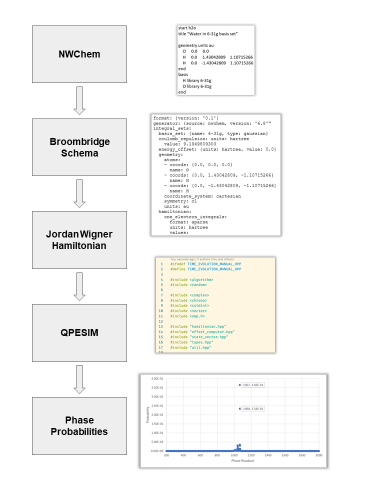
Figure 1: Flowchart describing the QPESIM simulation process. Systems are represented using NWChem and the corresponding Hamiltonian is extracted using the Broombridge Schema. Next, this Hamiltonian can be converted into an implementable Hamiltonian via the Jordan–Wigner transformation. QPESIM ingests this Hamiltonian to produce a series of phase probabilities, i.e. the probability of obtaining a certain phase from QPE. These phase probabilities can be used to produce an energy level estimate for the associated ansatz.

As seen in Table 1, the 15 orbital ground-state QPE simulation is relatively close to the analogous classical exact (FCI) solution and is lower than the previous 9 orbital simulations by $\sim$0.1 Hartree. The error relative to the full cc-pVDZ CCSDTQ (CC with singles, doubles, triples, and quadruples) Oliphant and Adamowicz (1991); Kucharski and Bartlett (1991); Piecuch and Adamowicz (1994) benchmark is reduced by more than a factor of three for the 15 orbital simulation compared to the previous smaller active space simulation. For the excited state, the larger active space lowers the total energy by 0.2–0.3 Hartree. As a result of the improved energies for the ground and excited state energies, the error of the excitation energy for the larger active space is reduced by more than a factor of two when compared to experiment and is only a few eVs higher than the benchmark EOMCCSD (Equation-of-motion CC with singles and doubles) Geertsen et al. (1989); Comeau and Bartlett (1993); Stanton and Bartlett (1993) and EOMCCSDT (EOMCC with singles, doubles, and triples) Kowalski and Piecuch (2001) excitation energies obtained with the full cc-pVDZ orbital space. We would also like to note that while previous simulations and EOMCC benchmarks used a slightly different geometry, the differences in energies due to the changes in geometry are insignificant compared to the change in energies due to the larger active space.

While larger active spaces can significantly improve results and expand the capabilities of quantum simulations, there is much value in techniques for compacting electronic correlation and reducing the dimensions of a problem through various techniques. A simple demonstration of this is seen when we replace the RHF orbitals in the active space with the 15 largest occupation MP2 natural orbitals for the ground state. Not only is the energy reduced by approximately 60 milliHartree compared to the analogous RHF case, but the improved energy is only 23 milliHartree from the benchmark CCSDTQ energy for the full orbital space. This error would further improve with natural orbitals from higher-order methods and approaches such as the downfolding techniques that we introduced in earlier studies.

Method	Orbitals	Energy
Ground State
QPEa	RHF (9 Orbitals)	-76.0591
QPE(p=14, r=5)	RHF (15 Orbitals)	-76.1612
QPE(p=14, r=10)b	nMP2 (15 Orbitals)	-76.2225
		-76.2187
		(-76.2207)
FCI	RHF (15 Orbitals)	-76.1482
CCSDTQc	RHF (24 Orbitals)	-76.2438
Core-level Excited State
QPEa	RHF (9 Orbitals)	-55.9517
QPE(p=14, r=5)	RHF (15 Orbitals)	-56.3076
Excitation Energies
QPEa	RHF (9 Orbitals)	547.15
QPE(p=14, r=5)	RHF (15 Orbitals)	540.24
EOMCCSDd	RHF (24 Orbitals)	538.40
EOMCCSDTe	RHF (24 Orbitals)	537.32
Experimentf	–	534.0

Table 1: Total energies (Hartree) for the ground ($1^{1}A_{1}$) and excited ($1a_{1}\rightarrow 4a_{1}$ transition) states of H₂O, along with their respective excitation energies (eV).

^aTaken from Ref. (47). ^bTwo neighboring phases with probabilities greater than 0.1 were identified within the same simulation. Both energies are reported along with a weighted average, in parenthesis, based on their respective probabilities. ^cThe CCSDTQ total energy for the full cc-pVDZ orbital space. ^dThe EOMCCSD cc-pVDZ excitation energy taken from Ref. (61). ^eThe EOMCCSDT cc-pVDZ excitation energy taken from Ref. (61). ^fExperimental excitation energy taken from Ref. (62)

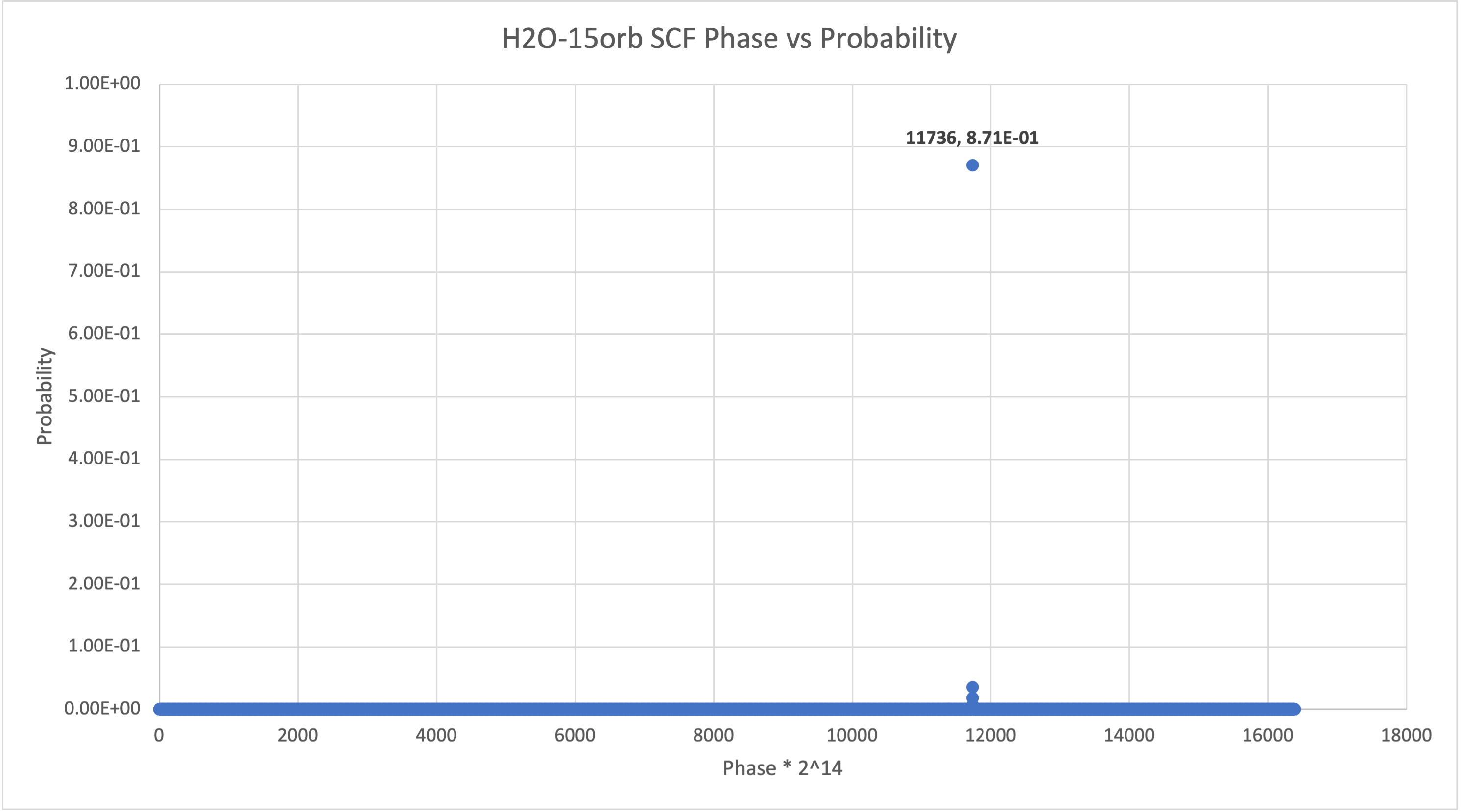
Figure 2: The phase/probability distribution for the ground state of H₂O, obtained using the 15 lowest-energy RHF orbitals. There is a primary peak at 11736 with probability 87.1%.

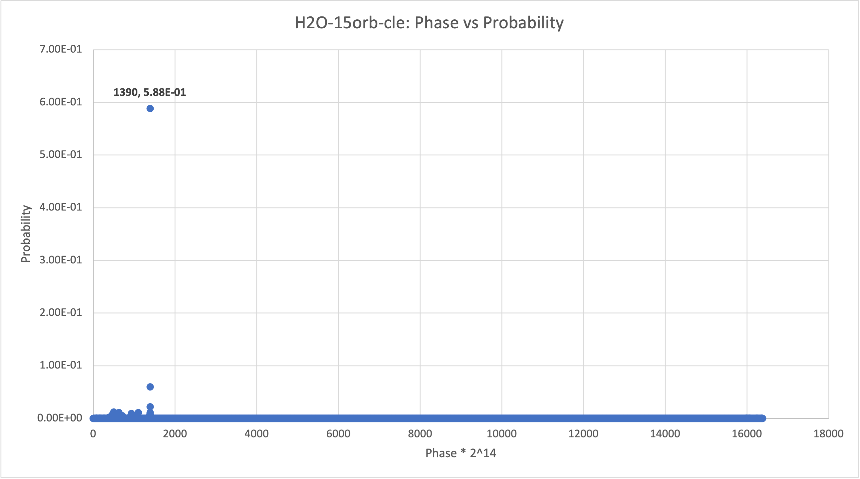
Figure 3: The phase/probability distribution for the lowest-energy core-level excited state of H₂O ($1a_{1}\rightarrow 4a_{1}$ transition), obtained using the 15 lowest-energy RHF orbitals. We observe a dominant phase of 1390 with probability 58.8% which was taken as the lone peak in our computation of the energy level.

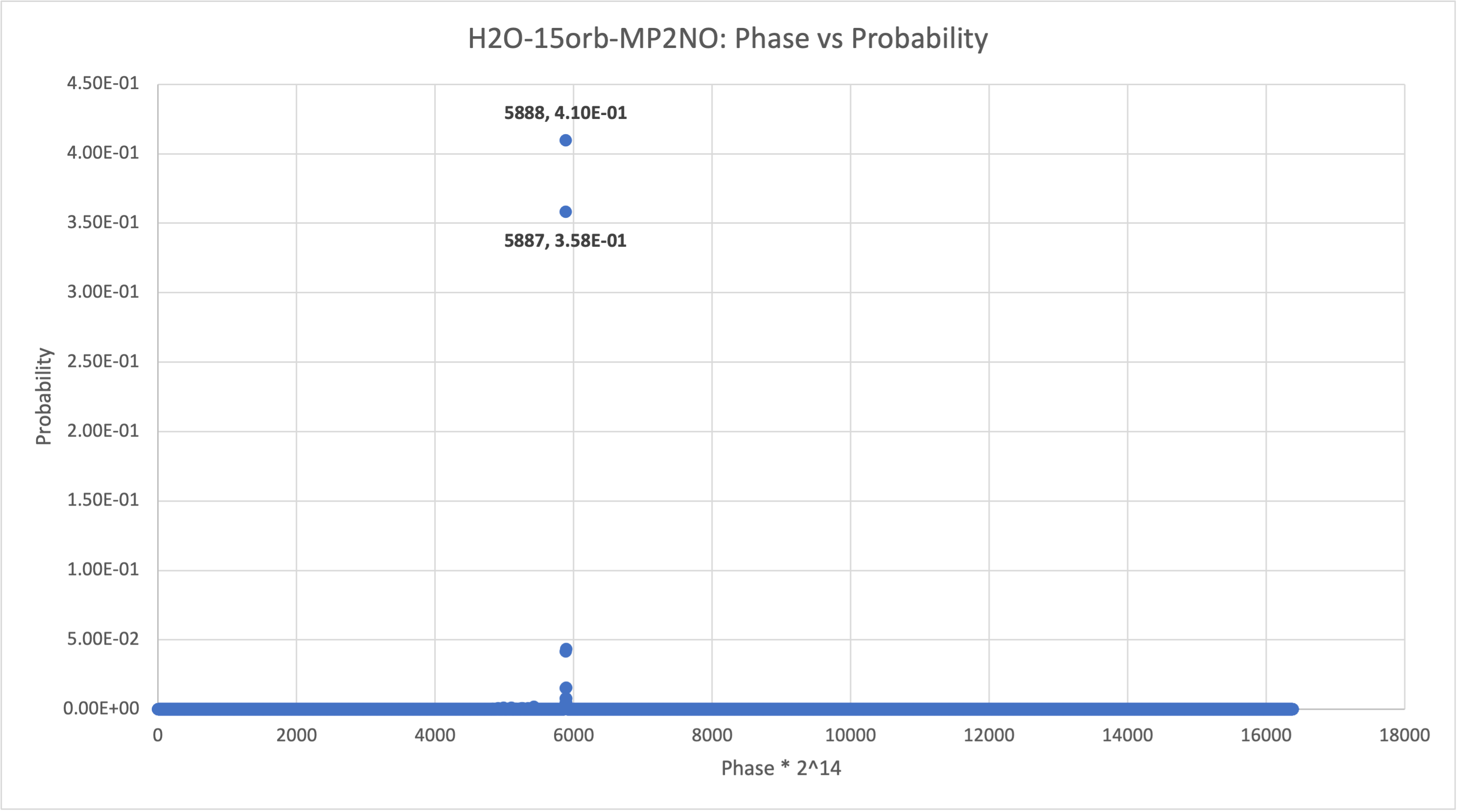
Figure 4: The phase/probability distribution for the ground state of H₂O, obtained using the 15 lowest-energy MP2 natural orbitals. We observe that the phase is split between two readouts: 5888 with probability 41.0% and 5887 with probability 35.8%. Table 1 contains the corresponding energies for these two phases, as well as the weighted average of these two readouts.

V Conclusion

In this paper, we demonstrated the versatility of the QPESIM code in applications to chemical problems. Our primary focus was on describing electronic states corresponding to various energy regimes. As a particular example, we chose the problem of calculating excitation energies corresponding to core-level excitation of the water molecule recently analyzed using the QPE algorithm. Our QPESIM implementation allowed for the utilization of significantly larger active spaces than previously possible. As a result, when using active space defined by 15 RHF orbitals, we could observe a significant two-fold reduction of computed core-level excitation energy error obtained in QPE simulations employing 9 RHF active orbitals when compared with experiment. The obtained QPE results for core-level excitation energy corresponding to the singly-excited core-level state of ${}^{1}A_{1}$ symmetry are in good agreement with the EOMCCSD results obtained with all orbitals being correlated.

In the QPESIM calculations for the ground-state energy of water molecules in equilibrium configurations, we also demonstrated the advantage of utilizing natural orbitals determined at the MP2 level. Using active space composed of 15 natural active orbitals, we achieved more than a three-fold reduction of error in correlation energy obtained in simulations involving 15 RHF active orbitals compared to the CCSDTQ results obtained for all orbitals being correlated.

There is an ongoing effort towards further optimization of the QPESIM code, which should enable QPE simulations of systems described by 20-25 active orbitals, which will enable us for the direct evaluation of the QPE performance compared to the results obtained with high-order CC/EOMCC methods for a broad class of electronic states.

VI Acknowledgement

The main part of this work was supported by the Quantum Science Center (QSC), a National Quantum Information Science Research Center of the U.S. Department of Energy (DOE). Part of this work was supported by the ”Embedding QC into Many-body Frameworks for Strongly Correlated Molecular and Materials Systems” project, which is funded by the U.S. Department of Energy, Office of Science, Office of Basic Energy Sciences (BES), the Division of Chemical Sciences, Geosciences, and Biosciences. C.K. thanks Nathan Wiebe for discussions about the nature of QPE-based algorithms for simulation.

References

- Coester (1958) Coester, F. Bound States of a Many-Particle System. Nucl. Phys. 1958, 7, 421–424.
- Coester and Kummel (1960) Coester, F.; Kummel, H. Short-Range Correlations in Nuclear Wave Functions. Nucl. Phys. 1960, 17, 477–485.
- Čížek (1966) Čížek, J. On the Correlation Problem in Atomic and Molecular Systems. Calculation of Wavefunction Components in Ursell-Type Expansion Using Quantum-Field Theoretical Methods. J. Chem. Phys. 1966, 45, 4256–4266.
- Paldus et al. (1972) Paldus, J.; Čížek, J.; Shavitt, I. Correlation Problems in Atomic and Molecular Systems. IV. Extended Coupled-Pair Many-Electron Theory and Its Application to the B Molecule. Phys. Rev. A 1972, 5, 50–67.
- Purvis and Bartlett (1982) Purvis, G.; Bartlett, R. A Full Coupled-Cluster Singles and Doubles Model: The Inclusion of Disconnected Triples. J. Chem. Phys. 1982, 76, 1910–1918.
- Koch and Jørgensen (1990) Koch, H.; Jørgensen, P. Coupled Cluster Response Functions. J. Chem. Phys. 1990, 93, 3333–3344.
- Paldus and Li (1999) Paldus, J.; Li, X. A Critical Assessment of Coupled Cluster Method in Quantum Chemistry. Adv. Chem. Phys. 1999, 110, 1–175.
- Crawford and Schaefer (2000) Crawford, T. D.; Schaefer, H. F. An introduction to coupled cluster theory for computational chemists. Reviews in computational chemistry 2000, 14, 33–136.
- Bartlett and Musiał (2007) Bartlett, R. J.; Musiał, M. Coupled-Cluster Theory in Quantum Chemistry. Rev. Mod. Phys. 2007, 79, 291–352.
- Mukherjee et al. (1975) Mukherjee, D.; Moitra, R. K.; Mukhopadhyay, A. Correlation problem in open-shell atoms and molecules. Mol. Phys. 1975, 30, 1861–1888.
- Kutzelnigg (1982) Kutzelnigg, W. Quantum chemistry in Fock space. I. The universal wave and energy operators. The Journal of Chemical Physics 1982, 77, 3081–3097.
- Stolarczyk and Monkhorst (1985) Stolarczyk, L. Z.; Monkhorst, H. J. Coupled-cluster method in Fock space. I. General formalism. Physical Review A 1985, 32, 725.
- Jeziorski and Paldus (1989) Jeziorski, B.; Paldus, J. Valence universal exponential ansatz and the cluster structure of multireference configuration interaction wave function. The Journal of chemical physics 1989, 90, 2714–2731.
- Rittby and Bartlett (1991) Rittby, C.; Bartlett, R. Multireference coupled cluster theory in Fock space. Theoretica chimica acta 1991, 80, 469–482.
- Kaldor (1991) Kaldor, U. The Fock space coupled cluster method: theory and application. Theoretica chimica acta 1991, 80, 427–439.
- Meissner (1998) Meissner, L. Fock-space coupled-cluster method in the intermediate Hamiltonian formulation: Model with singles and doubles. The Journal of chemical physics 1998, 108, 9227–9235.
- Jeziorski and Monkhorst (1981) Jeziorski, B.; Monkhorst, H. J. Coupled-cluster method for multideterminantal reference states. Phys. Rev. A 1981, 24, 1668–1681.
- Meissner et al. (1988) Meissner, L.; Jankowski, K.; Wasilewski, J. A coupled-cluster method for quasidegenerate states. Int. J. Quantum Chem. 1988, 34, 535–557.
- Pittner et al. (1999) Pittner, J.; Nachtigall, P.; Carsky, P.; Masik, J.; Hubac, I. Assessment of the single-root multireference Brillouin-Wigner coupled-cluster method: Test calculations on CH2, SiH2,and twisted ethylene. J. Chem. Phys. 1999, 110, 10275–10282.
- Mahapatra et al. (1998) Mahapatra, U. S.; Datta, B.; Mukherjee, D. A state-specific multi-reference coupled cluster formalism with molecular applications. Mol. Phys. 1998, 94, 157–171.
- Mahapatra et al. (1998) Mahapatra, U. S.; Datta, B.; Bandyopadhyay, B.; Mukherjee, D. In State-Specific Multi-Reference Coupled Cluster Formulations: Two Paradigms; Lowdin, P.-O., Ed.; Advances in Quantum Chemistry; Academic Press, 1998; Vol. 30; pp 163–193.
- Evangelista et al. (2007) Evangelista, F. A.; Allen, W. D.; III, H. F. S. Coupling term derivation and general implementation of state-specific multireference coupled cluster theories. J. Chem. Phys. 2007, 127, 024102.
- Lyakh et al. (2012) Lyakh, D. I.; Musiał, M.; Lotrich, V. F.; Bartlett, R. J. Multireference nature of chemistry: The coupled-cluster view. Chem. Rev. 2012, 112, 182–243.
- Kitaev (1997) Kitaev, A. Y. Quantum computations: algorithms and error correction. Russian Mathematical Surveys 1997, 52, 1191–1249.
- Nielsen and Chuang (2011) Nielsen, M. A.; Chuang, I. L. Quantum Computation and Quantum Information: 10th Anniversary Edition, 10th ed.; Cambridge University Press: New York, NY, USA, 2011.
- Luis and Peřina (1996) Luis, A.; Peřina, J. Optimum phase-shift estimation and the quantum description of the phase difference. Phys. Rev. A 1996, 54, 4564.
- Cleve et al. (1998) Cleve, R.; Ekert, A.; Macchiavello, C.; Mosca, M. Proc. R. Soc. Lond. A 1998, 454, 339–354.
- Berry et al. (2007) Berry, D. W.; Ahokas, G.; Cleve, R.; Sanders, B. C. Efficient quantum algorithms for simulating sparse Hamiltonians. Comm. Math. Phys. 2007, 270, 359–371.
- Childs (2010) Childs, A. M. On the relationship between continuous-and discrete-time quantum walk. Comm. Math. Phys. 2010, 294, 581–603.
- Seeley et al. (2012) Seeley, J. T.; Richard, M. J.; Love, P. J. The Bravyi-Kitaev transformation for quantum computation of electronic structure. J. Chem. Phys. 2012, 137, 224109.
- Wecker et al. (2015) Wecker, D.; Hastings, M. B.; Troyer, M. Progress towards practical quantum variational algorithms. Phys. Rev. A 2015, 92, 042303.
- Häner et al. (2016) Häner, T.; Steiger, D. S.; Smelyanskiy, M.; Troyer, M. High Performance Emulation of Quantum Circuits. SC ’16: Proceedings of the International Conference for High Performance Computing, Networking, Storage and Analysis. 2016; pp 866–874.
- Poulin et al. (2017) Poulin, D.; Kitaev, A.; Steiger, D. S.; Hastings, M. B.; Troyer, M. Fast quantum algorithm for spectral properties. arXiv preprint arXiv:1711.11025 2017,
- Berry et al. (2006) Berry, D. W.; Ahokas, G.; Cleve, R.; Sanders, B. C. Efficient Quantum Algorithms for Simulating Sparse Hamiltonians. Communications in Mathematical Physics 2006, 270, 359-371.
- Peruzzo et al. (2014) Peruzzo, A.; McClean, J.; Shadbolt, P.; Yung, M.-H.; Zhou, X.-Q.; Love, P. J.; Aspuru-Guzik, A.; O’brien, J. L. A variational eigenvalue solver on a photonic quantum processor. Nat. Commun. 2014, 5, 4213.
- McClean et al. (2016) McClean, J. R.; Romero, J.; Babbush, R.; Aspuru-Guzik, A. The theory of variational hybrid quantum-classical algorithms. New J. Phys 2016, 18, 023023.
- Romero et al. (2018) Romero, J.; Babbush, R.; McClean, J. R.; Hempel, C.; Love, P. J.; Aspuru-Guzik, A. Strategies for quantum computing molecular energies using the unitary coupled cluster ansatz. Quantum Sci. Technol. 2018, 4, 014008.
- Shen et al. (2017) Shen, Y.; Zhang, X.; Zhang, S.; Zhang, J.-N.; Yung, M.-H.; Kim, K. Quantum implementation of the unitary coupled cluster for simulating molecular electronic structure. Phys. Rev. A 2017, 95, 020501.
- Kandala et al. (2017) Kandala, A.; Mezzacapo, A.; Temme, K.; Takita, M.; Brink, M.; Chow, J. M.; Gambetta, J. M. Hardware-efficient variational quantum eigensolver for small molecules and quantum magnets. Nature 2017, 549, 242–246.
- Kandala et al. (2019) Kandala, A.; Temme, K.; Corcoles, A. D.; Mezzacapo, A.; Chow, J. M.; Gambetta, J. M. Error mitigation extends the computational reach of a noisy quantum processor. Nature 2019, 567, 491–495.
- Colless et al. (2018) Colless, J. I.; Ramasesh, V. V.; Dahlen, D.; Blok, M. S.; Kimchi-Schwartz, M. E.; McClean, J. R.; Carter, J.; de Jong, W. A.; Siddiqi, I. Computation of Molecular Spectra on a Quantum Processor with an Error-Resilient Algorithm. Phys. Rev. X 2018, 8, 011021.
- Huggins et al. (2020) Huggins, W. J.; Lee, J.; Baek, U.; O’Gorman, B.; Whaley, K. B. A non-orthogonal variational quantum eigensolver. New Journal of Physics 2020, 22, 073009.
- Cao et al. (2019) Cao, Y.; Romero, J.; Olson, J. P.; Degroote, M.; Johnson, P. D.; Kieferová, M.; Kivlichan, I. D.; Menke, T.; Peropadre, B.; Sawaya, N. P., et al. Quantum chemistry in the age of quantum computing. Chemical reviews 2019, 119, 10856–10915.
- Anand et al. (2021) Anand, A.; Schleich, P.; Alperin-Lea, S.; Jensen, P. W.; Sim, S.; Díaz-Tinoco, M.; Kottmann, J. S.; Degroote, M.; Izmaylov, A. F.; Aspuru-Guzik, A. A Quantum Computing View on Unitary Coupled Cluster Theory. arXiv preprint arXiv:2109.15176 2021,
- Valiev et al. (2010) Valiev, M.; Bylaska, E.; Govind, N.; Kowalski, K.; Straatsma, T.; Dam, H. V.; Wang, D.; Nieplocha, J.; Apra, E.; Windus, T.; de Jong, W. NWChem: A Comprehensive and Scalable Open-Source Solution for Large Scale Molecular Simulations. Comput. Phys. Comm. 2010, 181, 1477–1489.
- Apra et al. (2020) Apra, E.; Bylaska, E. J.; De Jong, W. A.; Govind, N.; Kowalski, K.; Straatsma, T. P.; Valiev, M.; van Dam, H. J.; Alexeev, Y.; Anchell, J., et al. NWChem: Past, present, and future. The Journal of chemical physics 2020, 152, 184102.
- Bauman et al. (2020) Bauman, N. P.; Liu, H.; Bylaska, E. J.; Krishnamoorthy, S.; Low, G. H.; Granade, C. E.; Wiebe, N.; Baker, N. A.; Peng, B.; Roetteler, M., et al. Toward Quantum Computing for High-Energy Excited States in Molecular Systems: Quantum Phase Estimations of Core-Level States. Journal of Chemical Theory and Computation 2020, 17, 201–210.
- Geertsen et al. (1989) Geertsen, J.; Rittby, M.; Bartlett, R. J. The Equation-of-Motion Coupled-Cluster Method: Excitation Energies of Be and CO. Chem. Phys. Lett. 1989, 164, 57–62.
- Comeau and Bartlett (1993) Comeau, D. C.; Bartlett, R. J. The Equation-of-Motion Coupled-Cluster Method. Applications to Open- and Closed-Shell Reference States. Chem. Phys. Lett. 1993, 207, 414–423.
- Stanton and Bartlett (1993) Stanton, J. F.; Bartlett, R. J. A Coupled-Cluster Based effective Hamiltonian Method for Dynamic Electric Polarizabilities. J. Chem. Phys. 1993, 99, 5178–5183.
- Whitfield et al. (2011) Whitfield, J. D.; Biamonte, J.; Aspuru-Guzik, A. Simulation of electronic structure Hamiltonians using quantum computers. Molecular Physics 2011, 109, 735-750.
- Hatano and Suzuki (2005) Hatano, N.; Suzuki, M. Quantum annealing and other optimization methods; Springer, 2005; pp 37–68.
- Svore et al. (2013) Svore, K. M.; Hastings, M. B.; Freedman, M. Faster phase estimation. arXiv preprint arXiv:1304.0741 2013,
- Abrams and Lloyd (1999) Abrams, D. S.; Lloyd, S. Quantum Algorithm Providing Exponential Speed Increase for Finding Eigenvalues and Eigenvectors. Physical Review Letters 1999, 83, 5162-5165.
- Kang et al. (2022) Kang, C.; Bauman, N.; Krishnamoorthy, S.; Kowalski, K. QPESIM. 2022; https://github.com/christopherkang/2022-qpesim.
- Hastings et al. (2014) Hastings, M. B.; Wecker, D.; Bauer, B.; Troyer, M. Improving quantum algorithms for quantum chemistry. arXiv preprint arXiv:1403.1539 2014,
- Oliphant and Adamowicz (1991) Oliphant, N.; Adamowicz, L. Coupled-cluster method truncated at quadruples. J. Chem. Phys. 1991, 95, 6645–6651.
- Kucharski and Bartlett (1991) Kucharski, S. A.; Bartlett, R. J. Recursive intermediate factorization and complete computational linearization of the coupled-cluster single, double, triple, and quadruple excitation equations. Theor. Chem. Acc. 1991, 80, 387–405.
- Piecuch and Adamowicz (1994) Piecuch, P.; Adamowicz, L. State-selective multireference coupled-cluster theory employing the single-reference formalism: Implementation and application to the H8 model system. J. Chem. Phys. 1994, 100, 5792–5809.
- Kowalski and Piecuch (2001) Kowalski, K.; Piecuch, P. The active-space equation-of-motion coupled-cluster methods for excited electronic states: Full EOMCCSDt. J. Chem. Phys. 2001, 115, 643–651.
- Brabec et al. (2012) Brabec, J.; Bhaskaran-Nair, K.; Govind, N.; Pittner, J.; Kowalski, K. Communication: Application of state-specific multireference coupled cluster methods to core-level excitations. The Journal of Chemical Physics 2012, 137, 171101.
- Schirmer et al. (1993) Schirmer, J.; Trofimov, A. B.; Randall, K. J.; Feldhaus, J.; Bradshaw, A. M.; Ma, Y.; Chen, C. T.; Sette, F. K-shell excitation of the water, ammonia, and methane molecules using high-resolution photoabsorption spectroscopy. Phys. Rev. A 1993, 47, 1136–1147.