Abstract

Most modern probabilistic generative models, such as the variational autoencoder (VAE), have certain indeterminacies that are unresolvable even with an infinite amount of data. Different tasks tolerate different indeterminacies, however recent applications have indicated the need for strongly identifiable models, in which an observation corresponds to a unique latent code. Progress has been made towards reducing model indeterminacies while maintaining flexibility, and recent work excludes many—but not all—indeterminacies. In this work, we motivate model-identifiability in terms of task-identifiability, then construct a theoretical framework for analyzing the indeterminacies of latent variable models, which enables their precise characterization in terms of the generator function and prior distribution spaces. We reveal that strong identifiability is possible even with highly flexible nonlinear generators, and give two such examples. One is a straightforward modification of iVAE (Khemakhem et al., 2020a, ); the other uses triangular monotonic maps, leading to novel connections between optimal transport and identifiability.

1 INTRODUCTION

In generative models, indeterminacy refers to the situation where the latent values underlying observations cannot be uniquely inferred from any amount of empirical evidence. It is a structural issue occurring in generative models such as the variational auto-encoder (VAE) (Kingma and Welling,, 2013) or independent component analysis (ICA) (Comon,, 1994; Hyvärinen and Pajunen,, 1999). For example, it is well known that even linear Gaussian models are plagued by a rotational indeterminacy, where arbitrary rotations of the latent space result in equivalent observation distributions. Modern nonlinear (deep) generative models inherit such indeterminacies and many more.

Characterizing and reducing the indeterminacies of generative models has been referred to as identifiability, and has been motivated as a way to address a variety of problems in representation learning such as disentangelment (Locatello et al.,, 2019; Hälvä et al.,, 2021; Yang et al.,, 2021; Klindt et al.,, 2021), posterior collapse (Wang et al.,, 2021), and causal representation learning (Wang and Jordan,, 2021; Schölkopf et al.,, 2021; Lu et al.,, 2022). Compared to linear models, which restrict indeterminacies to linear transformations of the latent space, nonlinear identifiability is more challenging, and has been the subject of much recent work.

Consider a prototypical generative model,

$$Z_{i}\sim P_{z}\;,\quad\epsilon_{i}\sim\mathcal{N}(0,\sigma^{2})\;,\quad X_{i}=f(Z_{i})+\epsilon_{i}\;,$$

where $P_{z}\in\mathcal{P}_{z}$ is a distribution on latent variables, $f\in\mathcal{F}$ is an injective generator function, and $X_{i}$ is an observation. Indeterminacies arise when more than one $(f,P_{z})$ pair give rise to the same marginal distribution on observations, due to transformations of the latent space. Despite the seemingly disparate approaches taken in recent work to reduce indeterminacy, an intuitive trade-off appears: as more structure is added to the model through $\mathcal{F}$ and $\mathcal{P}_{z}\textbf{}$, indeterminacy is reduced and hence stronger identifiability results are obtained. Our first contribution is a framework for analyzing indeterminacy that abstracts away model specifics and formalises the trade-off as a general phenomenon, described by separating indeterminacy transformations into two possible sources. The first source is the set of transports that turn one distribution in $\mathcal{P}_{z}$ into another; denote this set by $\mathcal{A}(\mathcal{P}_{z})$. The second source, $\mathcal{A}(\mathcal{F})$, is the set of automorphisms of the latent space formed from two functions in $\mathcal{F}$ as $f_{b}^{-1}\circ f_{a}$ (See Section 2.3 for details). The main result of the analysis is that model indeterminacies must belong to both sets.

Theorem (Informal Statement of Theorem 2.2).

The set of indeterminacy transformations of a generative model $(\mathcal{F},\mathcal{P}_{z})$ is precisely $\mathcal{A}(\mathcal{F})\cap\mathcal{A}(\mathcal{P}_{z})$.

This reduces the identifiability analysis for any suitable generative model to a well-defined mathematical problem. It also categorizes various methods to reduce indeterminacies in the model class—either constrain $\mathcal{F}$, as in linear models; constrain $\mathcal{P}_{z}$, e.g., non-Gaussians; or constrain both. Any of these approaches will reduce the size of the intersection. This describes many recent methods for nonlinear identifiability. Generator constraints include restrictions to certain optimal transport maps (Wang et al.,, 2021), sparsity (Moran et al.,, 2022; Zheng et al.,, 2022) and restrictions on the Jacobian (Gresele et al.,, 2021; Buchholz et al.,, 2022). Many methods also assume a diffeomorphic or analytic generator, which further reduces $\mathcal{A}(\mathcal{F})$. Direct constraints on $\mathcal{P}_{z}$ include non-Gaussianity (Stühmer et al.,, 2020) and mixture distributions (Kivva et al.,, 2022). More commonly, latent distribution constraints are formulated in terms of dependence on an auxiliary variable (Hyvärinen and Morioka,, 2016, 2017; Hyvärinen et al.,, 2018; Khemakhem et al., 2020a, ; Khemakhem et al., 2020b, ; Hälvä et al.,, 2021; Klindt et al.,, 2021), multiple views (Locatello et al.,, 2020), when latent variables are perturbed via interventions (Brehmer et al.,, 2022) or sparse mechanism shifts (Lachapelle et al.,, 2022; Ahuja et al., 2022b, ). As an application of our framework, we show explicitly in Section 4 how multiple environments (e.g., Khemakhem et al., 2020a, ) and multiple views (e.g., Locatello et al.,, 2020) can yield stronger identifiability, simply by reducing the set of indeterminacy transformations.

Despite the progress in the references above, each of the identifiability results contained therein are weak, in the sense that non-trivial indeterminacies remain. An unanswered question is what constraints are required for strong identifiability, that is, pointwise uniqueness of the latent representation. It has long been seen as unattainable without major sacrifices to model flexibility. For example, permutation and scaling indeterminacies are considered fundamental in ICA models (Comon,, 1994). Our second main contribution is to use our framework in a few different ways to specify strongly identifiable nonlinear models, without restrictive sacrifices in flexibility. The simplest is to freeze the latent distribution before training the generator, as is typically done in a VAE. Specifically, we show that freezing the priors in iVAE (Khemakhem et al., 2020a, ), either from the outset or after some initial training, yields strong identifiability—with no further constraints on the generator class—when data from distinct environments (auxiliary information) are used (Section 4). We also show that monotonic triangular flow generators (Huang et al.,, 2018; Jaini et al.,, 2019; Wehenlkel and Louppe,, 2019; Irons et al.,, 2022), which are universal transports between fully supported distributions, are strongly identifiable even with a single environment, and with any latent distribution (Section 5).

Even when strong identifiability is unachievable, weakly identifiable models may be useful for tasks that tolerate the remaining indeterminacies. Our third main contribution is to formally relate model identifiability to task identifiability in Section 3, providing precise conditions for when weak identifiability is good enough for identifiability of a particular downstream task, including some examples from the recent literature. One obvious conclusion is that strongly identifiable models are acceptable for any task based on the latent variables.

Before proceeding, we note that any notion of model identifiability is an asymptotic property not achievable with finite data. However, model identifiability is an important quality for statistical inference, and in particular is necessary for the typical consistency guarantees (van der Vaart,, 1998). Though future work is required to assess the finite-sample properties of identifiable models, empirical evidence shows that even weak identifiability can recover ground truths in simulation studies (Khemakhem et al., 2020a, ; Sorrenson et al.,, 2020; Lu et al.,, 2022).

Outline   In the rest of this section, we motivate our framework with two classical linear examples, and discuss identifiability at a high level from a downstream task-specific point of view, outlining when and what degree of identifiability is required. In Section 2, we define our mathematical framework and present our main technical results on model identifiability. After revisiting the task-specific view in detail in Section 3, we then apply the framework to analyze the auxiliary information setting in Section 4, showing in detail how the iVAE fits into the framework, and how it can be easily adapted for strong identifiability. In Section 5 we describe properties of triangular flows that yield strongly identifiable models, which can then be generalized to flows based on certain optimal transports.

1.1 Factor Analysis and Linear ICA

Factor analysis (Lawley and Maxwell,, 1962) is a linear generative model,

$$Z_{i}\sim\mathcal{N}(0,I_{d_{z}}),\;\quad\epsilon_{i}\sim\mathcal{N}(\mu,I_{d_{x}}),\;\quad X_{i}=F\,Z_{i}+\epsilon_{i}\;,$$

where $\epsilon_{i}{\perp\!\!\!\perp}Z_{i}$, and $F$ is a full-rank $d_{x}\times d_{z}$ matrix of so-called factor loadings. Here, $F$ is the only learnable parameter and $\mathcal{P}_{z}=\{\mathcal{N}(0,I_{d_{z}})\}$, a singleton. Linear ICA (Comon,, 1994) is structurally identical, but relaxes the assumption that $Z$ has a Gaussian distribution. Instead, it is parametrized by $(F,P_{z})$, where $F$ is again full rank, and $P_{z}$ is required to have independent components and is learned along with $F$ from data. In other words, $\mathcal{P}_{z}$ is some collection of fully supported distributions with independent components, typically excluding Gaussians.

It is well known that factor analysis suffers from a rotational indeterminacy due to the Gaussian $P_{z}$. On the other hand, Hastie et al., (2009) note that ICA is identical in form to factor analysis, but avoids the rotational indeterminacy via its non-Gaussian assumption. However, if scaling indeterminacies are fundamental to ICA (Hyvarinen et al.,, 2001), why are they ignored in factor analysis?

Factor analysis does not suffer from scaling indeterminacy due to a fundamental difference in how indeterminacies arise in these two models. The factor model fixes its Gaussian $P_{z}$, and the rotational indeterminacies in factor analysis can be characterized precisely as linear measure-preserving automorphisms of the standard Gaussian. Since scaling does not preserve the standard Gaussian, it is not an indeterminacy. On the other hand, ICA does not fix $P_{z}$. Due to this, any linear transformation of $P_{z}\in\mathcal{P}_{z}$ to another $P_{z}^{\prime}\in\mathcal{P}_{z}$ is an indeterminacy, and a result of Comon, (1994, Thm. 10) is that only scalings and permutations are possible when $\mathcal{P}_{z}$ contains all independent distributions excluding Gaussians.

Our Theorem 2.2 below generalizes these special cases. It can be used to show that indeterminacies are completely characterized as measure-preserving automorphisms for fixed latent distributions (as in factor analysis), and as measure-transporting isomorphisms within $\mathcal{P}_{z}$ otherwise (as in ICA). One takeaway is that strong identifiability appears to be much easier to obtain in the factor analysis setting. We investigate this further in Sections 4 and 5.

1.2 Why and How Much Identifiability

In the recent literature on generative model identifiability, the question of why we care about identifiability typically appeals to recovering ground truth latent factors (Khemakhem et al., 2020a, ; Ahuja et al., 2022a, ; Yang et al.,, 2021; Lu et al.,, 2022). Besides requiring a philosophical position that asserts the objective reality of the latent variables and that the model contains the “true” data generating distribution, the use of an unidentifiable model—unable to be uniquely resolved from any amount of empirical evidence—makes the recovery of “true” latent factors impossible without further, untestable assumptions about the model. Another perspective is to consider when model indeterminacies preserve certain observable quantities, for example distances between observations (Arvanitidis et al.,, 2018). More generally, we might judge the importance of model identifiability in terms of whether or not a model can be used for its intended purpose. This opens the possibility that in some cases, weak identifiability may be sufficient; in others, it may not. To our knowledge, a characterization of the distinction has not been formalized in this setting.

To address these questions, we take a pragmatic approach based on downstream tasks that use the inferred latent variables. Informally, a task $t$ is a function of the model parameters $(f,P_{z})$, of data, $\mathbf{x}_{m}=(x_{1},\dotsc,x_{m})$, and of a finite collection of points in the latent space, $\mathbf{z}_{n}=(z_{1},\dotsc,z_{n})$. There must be some procedure for selecting the latent points $\mathbf{z}_{n}$ represented by a selection function $\mathbf{z}_{n}=s(f,P_{z},\mathbf{x}_{m})$, e.g., $s(f,P_{z},\mathbf{x}_{m})\approx f^{-1}(\mathbf{x}_{m})$. The entire task is given by $t(f,P_{z},\mathbf{x}_{m},s(f,P_{z},\mathbf{x}_{m}))$.

Some examples are generating synthetic or counterfactual data by shifting inferred latent variables (Higgins et al.,, 2017), or causal discovery through independence tests (Monti et al.,, 2020; Khemakhem et al., 2020a, ; Lu et al.,, 2022). Both of these examples are studied in detail in Section 3. For a model to be useful for a task, the resulting task output should be the same for all generative model parameters $(f,P_{z})$ that yield the same marginal distribution for the observations (this is made precise in Section 3). For example, Fig. 1 illustrates a task that is constant on each set of points induced by the indeterminacy transformations (rotations). That guarantees that two fits of the same model to the same (infinite) data yield the same task values; weak model identifiability can be sufficient when the relevant task is insensitive to all model indeterminacies. Strongly identifiable models make all tasks trivially insensitive and therefore identifiable.

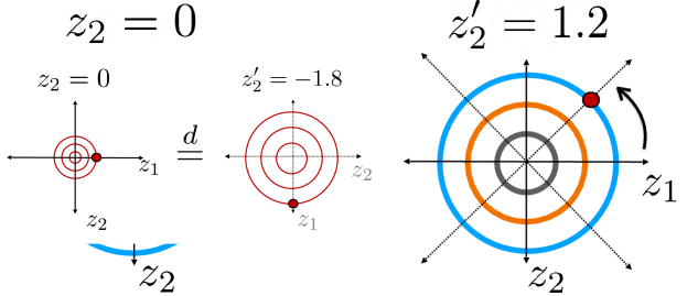
Figure 1: Rotational indeterminacy is fundamental in Gaussian i.i.d. models, where each point on the above orbits represent an equivalent solution. If a task gives constant output on each orbit, the task is identifiable even in the presence of model indeterminacies.

2 IDENTIFIABILITY IN GENERATIVE MODELS

Conceptually, our results are relatively simple, but some care is required to establish them rigorously. See Appendix C and Appendix D for technical background and proofs.

A Borel space $(\mathbf{X},\mathcal{B}(\mathbf{X}))$ is a topological space $\mathbf{X}$ equipped with the $\sigma$-algebra generated by its open sets, denoted $\mathcal{B}(\mathbf{X})$. All measurable spaces in this paper will be Borel spaces, and for convenience we leave the $\sigma$-algebra implicit in the notation, referring to the Borel space $(\mathbf{X},\mathcal{B}(\mathbf{X}))$ simply as $\mathbf{X}$. Let $\mathbf{Z}$ and $\mathbf{X}$ be two Borel spaces and $f\colon\mathbf{Z}\to\mathbf{X}$ a measurable function. If $f$ is bijective with measurable inverse then it is called a Borel isomorphism of $\mathbf{Z}$ and $\mathbf{X}$. If $\mathbf{X}=\mathbf{Z}$ then $f$ is a Borel automorphism. We denote the set of Borel automorphisms of $\mathbf{Z}$ as $\operatorname{Aut}(\mathbf{Z})$.

We will use the notation $\mathbf{X}$ and $\mathbf{Z}$ to represent the observable space and latent space, respectively. In practice, typically $\mathbf{X}=\mathbb{R}^{d_{x}}$ and $\mathbf{Z}=\mathbb{R}^{d_{z}}$, $d_{z}\leq d_{x}$. For clarity, we will usually refer to these specific spaces, where almost everywhere statements and probability densities are with respect to the Lebesgue measure; our results in Section 2 and Section 3 apply to generic Borel measure spaces. We write $f_{a}\mathrel{\mathop{=}\limits^{\vbox to0.75346pt{\kern-2.0pt\hbox{$\scriptstyle\text{\rm a.e.}$}\vss}}}f_{b}$ for measurable functions as shorthand for equality almost everywhere on their domain. The main objects of study in our theory are certain elements of $\operatorname{Aut}(\mathbf{Z})$, as follows.

Let $\mu$ and $\nu$ be two measures on $\mathbf{Z}$, and $A\in\operatorname{Aut}(\mathbf{Z})$. $A$ is called a $(\mu,\nu)$-measure isomorphism whenever $A_{\#}\mu=\nu$ (equiv.  $A^{-1}_{\#}\nu=\mu)$, and a $\mu$-measure preserving automorphism if $\mu=A_{\#}\mu=A^{-1}_{\#}\mu$.

2.1 Model Definition

We model observations denoted $x_{i}$ as i.i.d. realizations of a random variable $X$ with distribution $P_{x}$ on $\mathbf{X}$. Define a latent random variable $Z$ with corresponding realizations $z_{i}$, with distribution $P_{z}$ on the latent space $\mathbf{Z}$. We further assume the presence of some noise realization $\epsilon_{i}$ with some fixed distribution $P_{\epsilon}$ applied by some noise mechanism $g$. Let $f\colon\mathbf{Z}\to\mathbf{X}$ be a measurable function, which we call the generator. We define a generative model as,

$$Z_{i}\sim P_{z}\;,\quad\epsilon_{i}\sim P_{\epsilon}\;,\quad X_{i}=g(f(Z_{i}),\epsilon_{i})\;,$$ (1)

with $Z_{i}{\perp\!\!\!\perp}\epsilon_{i}$. For example, in a VAE or factor analysis, $\mathbf{X}$ and $\mathbf{Z}$ are Euclidean spaces, and $g(f(z),\epsilon)=f(z)+\epsilon$ is additive noise. We will not be concerned with inferring the noise. Instead, we work with the assumption that the noise distribution and mechanism are fixed and have null effect on the probabilistic properties of the model.

Assumption 1.

Assume that $g$ and $P_{\epsilon}$ are such that, with $\epsilon_{a}\mathrel{\mathop{=}\limits^{\vbox to0.75346pt{\kern-2.0pt\hbox{$\scriptstyle\text{\rm d}$}\vss}}}\epsilon_{b}$, $g(f(Z_{a}),\epsilon_{a})\mathrel{\mathop{=}\limits^{\vbox to0.75346pt{\kern-2.0pt\hbox{$\scriptstyle\text{\rm d}$}\vss}}}g(f(Z_{b}),\epsilon_{b})$ if and only if $f(Z_{a})\mathrel{\mathop{=}\limits^{\vbox to0.75346pt{\kern-2.0pt\hbox{$\scriptstyle\text{\rm d}$}\vss}}}f(Z_{b})$.

This assumption includes, for example, the noiseless case, and additive noise for a suitable noise distribution (e.g., Hälvä et al.,, 2021). It means that, for identifiability purposes, it is sufficient to analyze the noiseless case. We note that it rules out the possibility of discrete observations except in very limited cases; see Appendix B for a brief discussion of this point. Designing a generative model involves specifying parameter spaces for the generator and the prior. We denote these as $\mathcal{F}$, a set of measurable mappings $\mathbf{Z}\to\mathbf{X}$; and $\mathcal{P}_{z}$, a set of probability measures on $\mathbf{Z}$. For example, $\mathcal{P}_{z}$ could be a singleton, as in factor analysis. In ICA, $\mathcal{P}_{z}$ contains only distributions that factorize over its components.

We will also assume that the generators are bijective on their range, which is required to make the inverse problem of recovering latents well-defined, and is a standard assumption in the identifiability literature.

Assumption 2.

Assume that any $f\in\mathcal{F}$ is injective, and has the same image: for any $f_{a},f_{b}\in\mathcal{F}$, $f_{a}(\mathbf{Z})=f_{b}(\mathbf{Z}):=\mathcal{F}(\mathbf{Z})\subseteq\mathbf{X}$.

2.2 Model Indeterminacies

A generative model (1) induces a statistical model as

$$\mathcal{M}(\mathcal{F},\mathcal{P}_{z})=\{P_{\theta}\text{ on }\mathbf{X}\mid\theta=(f,P_{z})\in\mathcal{F}\times\mathcal{P}_{z}\}\;.$$ (2)

Classical parameter identifiability can be defined via an equivalence relation $\sim$ on parameter space, $\theta\sim\theta^{\prime}\iff P_{\theta}=P_{\theta^{\prime}}$. The equivalence classes of parameters induced by $\sim$ are denoted by $[\theta]:=\{\theta^{\prime}\colon P_{\theta}=P_{\theta^{\prime}}\}$, and a model is identifiable up to $[\theta]$. Some authors refer only to the previous case as partial or set identifiability (Tamer,, 2010), and reserve the term identifiability for the case that $[\theta]=\{\theta\}$. We refer to this latter case as strong identifiability. Parameter identifiability does not appear to contain any information about the latent values. We take classical parameter identifiability as our starting point to formulate an alternative definition tailored to latent variable indeterminacy. Specifically, we work with transformations of the latent space that yield different generators but that leave the marginal distribution of the data unchanged.

Definition 1.

For a model $\mathcal{M}(\mathcal{F},\mathcal{P}_{z})$, $A_{a,b}$ is an indeterminacy transformation at $\theta_{a},\theta_{b}$ if $P_{\theta_{a}}=P_{\theta_{b}}$ and $f_{a}\circ A_{a,b}^{-1}\mathrel{\mathop{=}\limits^{\vbox to0.75346pt{\kern-2.0pt\hbox{$\scriptstyle\text{\rm a.e.}$}\vss}}}f_{b}$. The indeterminacy set of a model $\mathcal{M}(\mathcal{F},\mathcal{P}_{z})$, denoted $\mathcal{A}(\mathcal{M})$, is the collection of all indeterminacy transformations of the model.

Definition 1 describes latent variable indeterminacy; it implies that if $\mathcal{A}(\mathcal{M})$ contains non-trivial transformations, any latent $z$ that generates $x=f(z)$ has an equivalent counterpart $A(z)$ for some $A\in\mathcal{A}(\mathcal{M})$. The identity map on $\mathbf{Z}$, $\textrm{id}_{z}$, is always (trivially) an indeterminacy transformation by taking $\theta_{a}=\theta_{b}$. A simple way to construct non-trivial candidate indeterminacy transformations at $\theta_{a}\neq\theta_{b}$ is by “pushing forward” and “pulling back” along the generators,

$$\vec{A}_{a,b}(z):=f_{b}^{-1}(f_{a}(z))\;,\quad z\in\mathbf{Z}\;.$$ (3)

It is possible to show that $\vec{A}_{a,b}\in\operatorname{Aut}(\mathbf{Z})$, and thus if transforming $\mathbf{Z}$ in this way results in $P_{\theta_{a}}=P_{\theta_{b}}$, then $\vec{A}_{a,b}$ is an indeterminacy transformation. We refer to $\vec{A}_{a,b}\colon\mathbf{Z}\to\mathbf{Z}$ as the generator transform between $\theta_{a}$ and $\theta_{b}$. It turns out that generator transforms characterize all the possible indeterminacy transformations of a model—though not every generator transform is an indeterminacy transformation.

Lemma 2.1.

Let $\theta_{a}=(f_{a},P_{z,a})$ and $\theta_{b}=(f_{b},P_{z,b})$ be two parametrizations of a generative model with resulting marginal distributions $P_{\theta_{a}}$ and $P_{\theta_{b}}$. Then, $P_{\theta_{a}}=P_{\theta_{b}}$ if and only if $\vec{A}_{a,b}$ is a $(P_{z,a},P_{z,b})$-measure isomorphism. Furthermore, any $A\in\operatorname{Aut}(\mathbf{Z})$ is an indeterminacy transformation at $\theta_{a},\theta_{b}$ (Definition 1) if and only if $A\mathrel{\mathop{=}\limits^{\vbox to0.75346pt{\kern-2.0pt\hbox{$\scriptstyle\text{\rm a.e.}$}\vss}}}\vec{A}_{a,b}$, and therefore all indeterminacy transformations $A_{a,b}$ must be $(P_{z,a},P_{z,b})$-measure isomorphisms.

Lemma 2.1 is the technical foundation for the rest of the paper, and can be interpreted as an existence and uniqueness result, as follows. $\vec{A}_{a,b}$ is a distinguished indeterminacy transformation at $\theta_{a}$, $\theta_{b}$ that always exists; it is probabilistically equivalent to all other indeterminacy transformations, making it essentially unique. It implies that two parameterizations $\theta_{a},\theta_{b}$ induce the same marginal distribution on observations if and only if one can transport between the two latent measures in $\mathcal{P}_{z}$ by pushing and pulling along the generators. Not only are there no other non-equivalent indeterminacy transformations, but $A_{a,b}$ cannot be an indeterminacy transformation for any other parameters $\theta_{c},\theta_{d}$ unless $\vec{A}_{a,b}=f_{b}^{-1}\circ f_{a}\mathrel{\mathop{=}\limits^{\vbox to0.75346pt{\kern-2.0pt\hbox{$\scriptstyle\text{\rm a.e.}$}\vss}}}f_{d}^{-1}\circ f_{c}=\vec{A}_{c,d}$. Both of these properties follow directly from the injectivity of the generators; relaxing 2 would require a substantially different theory than the one developed here.

2.3 Characterizing Model Identifiability

Let $\widetilde{\textrm{id}}_{z}$ denote the set of all Borel automorphisms that are equal a.e. to the identity mapping on $\mathbf{Z}$. If $\mathcal{A}(\mathcal{M})=\widetilde{\textrm{id}}_{z}$, then $f_{a}\mathrel{\mathop{=}\limits^{\vbox to0.75346pt{\kern-2.0pt\hbox{$\scriptstyle\text{\rm a.e.}$}\vss}}}f_{b}$ for all $\theta_{a},\theta_{b}$ with $P_{\theta_{a}}=P_{\theta_{b}}$. We use this to define the appropriate notion of identifiability.

Definition 2.

A generative model $\mathcal{M}(\mathcal{F},\mathcal{P}_{z})$ is weakly identifiable up to $\mathcal{A}(\mathcal{M})$, or $\mathcal{A}(\mathcal{M})$-identifiable, if its indeterminacy transformations are $\mathcal{A}(\mathcal{M})$. If $\mathcal{A}(\mathcal{M})=\widetilde{\textrm{id}}_{z}$, then the model is strongly identifiable.

Strong identifiability means that $f_{a}(z)=f_{b}(z)$ for all $z\in\mathbf{Z}$ outside of a set of measure zero. If $f_{a},f_{b}$ are continuous functions, this implies that $f_{a}(z)=f_{b}(z)$ for all $z\in\mathbf{Z}$, assuming the reference measure has full support. This definition is in correspondence to the classical definition, in the sense that the equivalence classes $[\theta]$ correspond to subsets of $\mathcal{A}(\mathcal{M})$ (see Proposition A.2 for details). Note that when the generator is further parameterized (for example via deep neural networks), this identifiability does not necessarily pass to the generator parameters (network weights). Rather, we use this as a proxy to make the notion of latent variable recoverability precise.

Lemma 2.1 gives a necessary and sufficient condition for two parameterizations to correspond to the same marginal distribution on observations. It also documents the cases in which $P_{\theta_{a}}$ cannot be equal to $P_{\theta_{b}}$, and allows us to construct the set of model indeterminacies $\mathcal{A}(\mathcal{M})$ as indeterminacies generated by $\mathcal{F}$ and $\mathcal{P}_{z}$. To that end, define the following subsets of $\operatorname{Aut}(\mathbf{Z})$ induced by the generative model,

$$\mathcal{A}(\mathcal{F})=\{A\in\operatorname{Aut}(\mathbf{Z})\mid\exists f_{a},f_{b}\in\mathcal{F}\text{ s.t. }A\mathrel{\mathop{=}\limits^{\vbox to0.75346pt{\kern-2.0pt\hbox{$\scriptstyle\text{\rm a.e.}$}\vss}}}f_{b}^{-1}\circ f_{a}\}$$

$$\mathcal{A}(\mathcal{P}_{z})=\{A\in\operatorname{Aut}(\mathbf{Z})\mid\exists P_{a},P_{b}\in\mathcal{P}_{z}\text{ s.t. }A_{\#}P_{a}=P_{b}\}\;.$$

$\mathcal{A}(\mathcal{F})$ consists of all possible indeterminacy transforms constructed from $\mathcal{F}$, which are a.e. equivalent to the generator transforms. $\mathcal{A}(\mathcal{P}_{z})$ consists of all possible isomorphisms between measures in $\mathcal{P}_{z}$. Both sets always include $\widetilde{\textrm{id}}_{z}$ by taking $f_{a}=f_{b}$ and $P_{a}=P_{b}$. The indeterminacies of the model are precisely their intersection.

Theorem 2.2.

The generative model $\mathcal{M}(\mathcal{F},\mathcal{P}_{z})$ is identifiable up to $\mathcal{A}(\mathcal{M})=\mathcal{A}(\mathcal{F})\cap\mathcal{A}(\mathcal{P}_{z})$. In particular, it is strongly identifiable if and only if $\mathcal{A}(\mathcal{F})\cap\mathcal{A}(\mathcal{P}_{z})=\widetilde{\textrm{id}}_{z}$.

This expresses the identifiability of a generative model in terms of the indeterminacy transforms induced by its parameter spaces. In particular, all model indeterminacies must be transports between distributions in $\mathcal{P}_{z}$ that can be constructed by pushing and pulling along generators from $\mathcal{F}$ as $f_{b}^{-1}\circ f_{a}$. These are the scaling and permutation matrices in the linear ICA example from Section 1.1. When $\mathcal{P}_{z}$ is a singleton $\{P_{z}\}$ as in factor analysis, they are $P_{z}$-measure-preserving automorphisms, such as the rotation matrices preserving the standard Gaussian.

2.4 Beyond Linear Generators

Theorem 2.2 exposes the structure of unidentifiability and indicates that there may be approaches to specifying strongly identifiable non-linear generative models. It suggests that model identifiability strengthens as we increase the number of constraints on $\mathcal{F}$, $\mathcal{P}_{z}$, or both, until the intersection $\mathcal{A}(\mathcal{F})\cap\mathcal{A}(\mathcal{P}_{z})$ contains only the identity. We demonstrate examples of leaving the generator unconstrained and only constraining $\mathcal{A}(\mathcal{P}_{z})$, as well as a triangular constraint on $\mathcal{A}(\mathcal{F})$ in Sections 4 and 5, respectively.

3 TASK IDENTIFIABILITY

In the literature on model identifiability, practical implications are often ignored. How does model identifiability relate to the intended uses of a model after it is fit to data? In practice, one may have a model that is only weakly identifiable but that still allows some tasks to be identified. That is, an unidentifiable model may still be useful for some tasks. For example, a causal estimand may still be identified without identification of the full causal model. For other tasks, an unidentifiable model is not useful. We make this idea precise before giving some examples from the literature.

Let $\mathbf{x}_{m}=(x_{1},\dotsc,x_{m})$ be a finite collection of points in $\mathbf{X}$ (e.g., $m$ observations), and recall that $\theta=(f,P_{z})$. Define a task as a pair of functions $(s,t)$: the function $s(\theta,\mathbf{x}_{m})\in\mathbf{Z}^{n}$ selects a set of $n$ points in the latent space to use for the task, e.g., estimates of $f^{-1}(x_{i})$; and $t\colon\mathcal{F}\times\mathcal{P}_{z}\times\mathbf{X}^{m}\times\mathbf{Z}^{n}\to\mathbf{T}$ generates the task output as $t(\theta,\mathbf{x}_{m},s(\theta,\mathbf{x}_{m}))$. Here, $\mathbf{T}$ is the task output space, such as $\mathbf{T}=\mathbf{X}$ for sample generation. We consider a task to be identifiable if two equivalent model fits produce the same task output.

Definition 3.

A task $(s,t)$ is identifiable at $[\theta]$ if, for all $\theta\sim\theta^{\prime}$ and $\mathbf{x}_{m}\in\mathbf{X}^{m}$,

$$t(\theta,\mathbf{x}_{m},s(\theta,\mathbf{x}_{m}))=t(\theta^{\prime},\mathbf{x}_{m},s(\theta^{\prime},\mathbf{x}_{m}))\;.$$ (4)

A task is (globally) identifiable if it is identifiable at all $[\theta]$.

This captures the idea that two different research groups may obtain different but equivalent model fits ($\theta$ and $\theta^{\prime}$) from the same data, and still reach the same conclusion for a task. Before proceeding, we give some examples.

Tasks Without Reference to Observations   Consider two labs with different but equivalent models, $\theta_{a}\sim\theta_{b}$. Now both labs set $s(\theta,\mathbf{x}_{m})=c$, without reference to observations. This could, for example, correspond to a ‘do’ intervention when $\mathbf{Z}$ is endowed with a causal model (Yang et al.,, 2021; Shen et al.,, 2022; Lu et al.,, 2022). As the task output, each lab generates a synthetic observation, $f_{a}(c)$ and $f_{b}(c)$. Without strong model identifiability, in general $f_{a}(c)\neq f_{b}(c)$ and the task is unidentifiable due to the fact that the value $c$ has no inherent meaning in either model. Tasks $t(\theta,\mathbf{x}_{m},c)$ will not be identifiable in general: the selection of latent points must incorporate the transformation of $\mathbf{Z}$ that occurs when $\theta_{a}\mapsto\theta_{b}$; only if the task output is constant across all equivalent $\theta$ will it be identifiable.

Disentanglement and Latent Shifts   A common demonstration of disentanglement is to select a latent variable $s(\theta,x_{i})=f^{-1}(x_{i})$ corresponding to an observation $x_{i}$, apply a shift $\delta$ along a latent dimension $k$ (with unit vector $e_{k}$), and then generate synthetic data $t_{\delta e_{k}}(\theta,x_{i},s(\theta,x_{i}))=f(\delta e_{k}+f^{-1}(x_{i}))$ for a sequence of different values of $\delta$ (e.g., Higgins et al.,, 2017; Lu et al.,, 2022). For most models, this task is not identifiable. To see why, observe that task identifiability requires

$$f_{a}( \delta e_{k}+f_{a}^{-1}(x))=f_{b}(\delta e_{k}+f_{b}^{-1}(x))$$

$$=f_{a}(\vec{A}^{-1}_{a,b}(\delta e_{k}+\vec{A}_{a,b}(f_{a}^{-1}(x))))\;.$$

In general, this will not be the case unless

$$\vec{A}^{-1}_{a,b}( \delta e_{k}+\vec{A}_{a,b}(f_{a}^{-1}(x))=\delta e_{k}+f_{a}^{-1}(x)\;.$$

That is, $\vec{A}_{a,b}$ must commute with $\delta e_{k}$. If that property is to hold for all $\delta$, $e_{k}$, and $x$ then $\vec{A}_{a,b}$ must be itself a translation.

Independence Testing and Causal Discovery    In applications of (nonlinear) ICA to causal discovery, tests for independence between observed variables and components of latent variables are conducted (Monti et al.,, 2020; Khemakhem et al., 2020a, ). In the simplest case, the goal is to determine the causal direction between two observed variables, $X_{1},X_{2}$. After fitting a model with independent latent components, pair-wise independence tests are conducted; if $X_{1}$ is a cause of $X_{2}$ and not vice versa, then $X_{1}$ will be independent of the second component of the corresponding latent variable, $f^{-1}(X_{1},X_{2})_{2}$. The task, based on observations $(x_{i})_{i=1}^{N}=(x_{i,1},x_{i,2})_{i=1}^{N}$ is then $s(\theta_{a},(x_{i})_{i=1}^{N})=(f_{a}^{-1}(x_{i}))_{i=1}^{N}$ and

$$t(\theta_{a}, (x_{i})_{i=1}^{N},s(\theta_{a},(x_{i})_{i=1}^{N}))$$

$$=\text{IndTest}((x_{i,1})_{i=1}^{N},(f_{a}^{-1}(x_{i,1},x_{i,2})_{2})_{i=1}^{N})\;.$$

If the model is identifiable up to component-wise transformations then $f_{a}^{-1}(x_{i,1},x_{i,2})_{2}=h(f_{b}^{-1}(x_{i,1},x_{i,2})_{2})$, for some function $h\colon\mathbb{R}\to\mathbb{R}$. Since two real-valued random variables $U,V$ are independent if and only if all transformations $k(U),k^{\prime}(V)$ are independent, this task remains identifiable under component-wise indeterminacies.

Define a local subset of indeterminacy transformations as $\mathcal{A}(\mathcal{M})|_{\theta}=\{A\in\mathcal{A}(\mathcal{M})\colon P_{\theta}=P_{A\theta}\}$, and $A\theta=(f\circ A^{-1},A_{\#}P_{z})$. Our main result on task identifiability is an application of Proposition A.2.

Proposition 3.1.

A task $(s,t)$ is identifiable at $[\theta]$ if and only if, for each $\mathbf{x}_{m}\in\mathbf{X}^{m}$,

$$t(\theta,\mathbf{x}_{m},s(\theta,\mathbf{x}_{m})) =t(A\theta,\mathbf{x}_{m},s(A\theta,\mathbf{x}_{m}))\;,$$ (5)

for each $A\in\mathcal{A}(\mathcal{M})|_{\theta}$. A sufficient condition for $(s,t)$ to be identifiable at $[\theta]$ is hence if the following holds for each $A\in\mathcal{A}(\mathcal{M})|_{\theta}$ and $\mathbf{x}_{m}\in\mathbf{X}^{m}$:

$$t(\theta,\mathbf{x}_{m},\mathbf{z}_{n})=t(A\theta,\mathbf{x}_{m},A(\mathbf{z}_{n}))$$ (6)

$$\textrm{and}\quad s(A\theta,\mathbf{x}_{m})=A(s(\theta,\mathbf{x}_{m}))\;.$$

Clearly, any task is identifiable if $\mathcal{M}$ is strongly identifiable: $\mathcal{A}(\mathcal{M})|_{\theta}=\mathcal{A}(\mathcal{M})=\widetilde{\textrm{id}}_{z}$. Weak identifiability may be enough depending on the task, Proposition 3.1 gives sufficient conditions based on the symmetries implied by $\mathcal{A}(\mathcal{M})$. In the next two sections, we apply the theory of Section 2 to obtain strongly identifiable models.

4 GENERATIVE MODELS IN MULTIPLE ENVIRONMENTS

Suppose data arise from environments indexed by $e\in E$, where $E$ is an arbitrary set, and the environment label is assumed to be deterministic (i.e., known, or observed without noise). Each environment corresponds to a different observation random variable $X^{e}\sim P_{x}^{e}$ on a shared observation space $\mathbf{X}$. This is reflected in the generative model as $|E|$ distinct distributions on latent variables, $Z^{e}\sim P_{z}^{e}$ on a shared latent space $\mathbf{Z}$. Crucially, each environment shares the same generator $f$. We denote the generative model $\mathcal{M}(\mathcal{F},\{\mathcal{P}_{z}^{e}\}_{e\in E})$ specified as, for each $e\in E$,

$$Z_{i}\sim P_{z}^{e}\;,\ \epsilon_{i}^{e}\sim P_{\epsilon}\;,\ X_{i}^{e}=g(f(Z_{i}^{e}),\epsilon_{i}^{e})\;,$$ (7)

with $Z_{i}{\perp\!\!\!\perp}\epsilon_{i}^{e}$ in each environment. In general, we do not assume that observations from different environments are paired in any way besides sharing a generator, e.g., they may be from separate datasets.

We use the multiple environments set-up in the same way as auxiliary information in iVAE. The definition of identifiability is subtly different here, but its implications for latent variable indeterminacy remain the same (see Section D.4 for details).

Corollary 4.1.

The generative model $\mathcal{M}(\mathcal{F},\{\mathcal{P}_{z}^{e}\}_{e\in E})$ is identifiable up to

$$\mathcal{A}(\mathcal{F})\cap\left(\cap_{e\in E}\mathcal{A}(\mathcal{P}_{z}^{e})\right).$$ (8)

We note that permutations of the environments are ruled out because the environments are assumed to be known. Clearly, the indeterminacy set shrinks with each environment added, formalizing why auxiliary information has such significant benefits for identifiability. As a demonstration, we recast iVAE under this framework and present the necessary modification for strong identifiability in Sections 4.2 and 4.3 (see LABEL:proofs:esm for a similar exercise for the results of Ahuja et al., 2022a ).

4.1 Multiple Views

A result similar to Corollary 4.1 can be obtained under different modelling assumptions similar to those made by Gresele et al., (2019); Locatello et al., (2020). Specifically, we assume here finitely many observed views of each latent variable, indexed by the finite set $E$. We study the following model, denoted by $\mathcal{M}(\{\mathcal{F}^{e}\}_{e\in E},\mathcal{P}_{z})$: for $e\in E$,

$$Z_{i}\sim P_{z}\;,\quad\epsilon_{i}^{e}\sim P_{\epsilon}^{e}\;,\quad X_{i}^{e}=g^{e}(f^{e}(Z_{i}),\epsilon_{i}^{e})\;,$$ (9)

with $Z_{i}{\perp\!\!\!\perp}\epsilon^{e}_{i}$. Here, for fixed $i$, each observed view $X_{i}^{e}$, $e\in E$, is generated by a shared latent variable $Z_{i}$, and hence the observations are necessarily grouped across environments (unlike the multiple environments setting). Each view $X_{i}^{e}$ can have a different observation space $\mathbf{X}^{e}$ with its own generator $f^{e}\in\mathcal{F}^{e}$, e.g., an image and its caption.

Again, the definition of identifiability here changes, but the implications for latent variable indeterminacy are identical. Intuitively, identification in any of the views yields identification of the generating latent (Section D.5).

Corollary 4.2.

The generative model $\mathcal{M}(\{\mathcal{F}^{e}\}_{e\in E},\mathcal{P}_{z})$ is identifiable up to

$$(\cap_{e\in E}\mathcal{A}(\mathcal{F}^{e}))\cap\mathcal{A}(\mathcal{P}_{z}).$$ (10)

This can be useful when, for example, when we have access to a lower-dimensional view (e.g., clinical data) which we might fit using an identifiable triangular flow (as developed in Section 5), in addition to a higher-dimensional view (e.g., genomics data), which can be reconstructed using a VAE.

4.2 (Weakly) Identifiable VAE

In the iVAE model (Khemakhem et al., 2020a, ), the latent variable distribution varies via an auxillary variable $u$, for example a time index (Hyvärinen et al.,, 2018). The prior is parameterized as an exponential family density on $\mathbf{Z}=\mathbb{R}^{d_{z}}$,

$$p(z;\eta(u))=m(z)\exp(\eta(u)^{\top}T(z)-a(\eta(u)),$$ (11)

with functional parameters $\eta$, $T$ taking values in $\mathbb{R}^{K}$. We denote this distribution as $\mathcal{E}_{m}(\eta(u),T)$. Note that this means the prior is explicitly inferred from the data, contrary to a standard VAE. The remainder of the model design follows (7) with additive noise. We note that Khemakhem et al., 2020a assumed the distribution to factorize over dimensions of $Z$ (as in ICA), but that is not necessary, an observation also made recently in Lu et al., (2022).

The main identifiability result of Khemakhem et al., 2020a (their Thm. 1) says that for two parametrizations $(f_{a},T_{a},\eta_{a})$ and $(f_{b},T_{b},\eta_{b})$, if there exist points $u_{0},u_{1},\dots u_{K}$ such that $\{\eta_{a}(u_{i})-\eta_{a}(u_{0})\}_{i=1}^{K}$ are linearly independent and span the latent space (and likewise for $\eta_{b})$, then there are an invertible matrix $L$ and offset vector $\mathbf{c}$ such that for all $x$,

$$T_{a}(f_{a}^{-1}(x))=L^{\top}T_{b}(f_{b}^{-1}(x))+\mathbf{c}.$$ (12)

Our framework allows us to show that this is purely a result of the following property of exponential families.

Proposition 4.3.

Suppose that $A\in\operatorname{Aut}(\mathbf{Z})$ is a $(\mathcal{E}_{m}(\eta_{a}(u_{i}),T_{a}),\mathcal{E}_{m}(\eta_{b}(u_{i}),T_{b})$-measure isomorphism for each $i=0,1,\dots,K$. Suppose that both $\{\eta_{a}(u_{i})\}_{i=0}^{K}$ and $\{\eta_{b}(u_{i})\}_{i=0}^{K}$ are linearly independent. Then,

$$T_{b}(A(z))=L^{\top}T_{a}(z)+\mathbf{d},$$ (13)

almost everywhere, where $L$ is a $K\times K$ invertible matrix and $d$ is a $K$-dimensional vector not depending on $x$.

Although the arguments made in the proof of the proposition are similar to those originally presented in Khemakhem et al., 2020a , our framework indicates that identifiability is a result purely of the exponential family form of the prior—neither diffeomorphic decoders nor independent components are needed. Further assuming that $f$ is diffeomorphic reduces $\mathcal{A}(\mathcal{F})$, leading to the stronger identifiability results of Theorems 2 and beyond in (Khemakhem et al., 2020a, ).

4.3 (Strongly) Identifiable VAE

In this section, we show how fixed priors, i.e., a nonlinear factor analysis take on VAEs, can lead to strong identifiability. By definition, with fixed latent distribution $P_{z}$, $\mathcal{A}(\{P_{z}\})$ is the set of $P_{z}$-preserving automorphisms. However, constructing distributions such that the only automorphism is the identity is in general very difficult; non-trivial measure automorphisms, such as via the Darmois construction, almost always exist (see Gresele et al.,, 2021, for an example). On the other hand, we show that multiple environments provide a simple solution to this problem.

We denote a set of full-rank exponential family densities indexed by $\eta\in\mathbb{R}^{K}$ as

$$\mathcal{E}_{m,T}=\{p_{\eta}(z)=m(z)\exp{(\eta^{\top}T(z)-a(\eta))}\mid\eta\in\mathbb{R}^{K}\}\;.$$ (14)

We refer to a particular distribution in such a set as $\mathcal{E}_{m,T}(\eta)$. Compared to the isomorphisms in Proposition 4.3, there is a stronger result characterizing the automorphisms of collections of exponential families.

Proposition 4.4.

Let $\mathcal{E}_{m,T}$ be as in (14), with $m$ strictly positive. Let $\eta_{i}\in\mathbb{R}^{K}$ for $i=0,1,\dots,K$ and suppose $A\in\operatorname{Aut}(\mathbb{R}^{d_{z}})$ is a $\mathcal{E}_{m,T}(\eta_{i})$-measure preserving automorphism for each $\eta_{i}$. Then, arranging $\eta_{i}$ into the rows of a matrix $M$, we have

$$(T(z)-T(A(z)))\in\textrm{ker}M,\ a.e.$$ (15)

Figure 2 illustrates (15). The proposition provides a characterization that can be specialized in several ways. Firstly, the only shared automorphism for each distribution from a suitably fixed exponential family $\mathcal{E}_{m,T}$ whose parameters form a basis of $\mathbb{R}^{K}$ is the identity (under $T$). Strong identifiability follows when these are fixed as the priors.

Theorem 4.5.

Let $\mathcal{M}(\mathcal{F},\{\mathcal{P}_{z}^{e}\}_{e\in E})$ be the multiple environments model described in (7), with $\mathbf{Z}=\mathbb{R}^{d_{z}}$. For a subset of environments $E^{*}\subset E$, with $|E^{*}|=K+1$, fix $P_{z}^{e}=\mathcal{E}_{m,T}(\eta_{e})$ with $m$ strictly positive and $T$ injective in at least one dimension, and such that the corresponding parameters $\{\eta_{e}\}_{e\in E^{*}}$ span $\mathbb{R}^{K}$. Then $\mathcal{M}(\mathcal{F},\{\mathcal{P}_{z}^{e}\}_{e\in E})$ is strongly identifiable.

In fact, we do not require a spanning set of environments for a useful characterization of the indeterminacy. A second specialization of Proposition 4.4 is in the case of Gaussian priors. In such a setting, assuming common covariances across environments, the model is identifiable up to arbitrary transformations on the dimensions not spanned by the environment means $\mu_{e}$; see Section D.9 for details.

Figure 2: The indeterminacy set (under the sufficient statistic) in red for parameter vectors $\eta_{1},\eta_{2}$.

4.4 Fixed versus Learned Distributions

In ICA compared to factor analysis (Section 1.1), and now iVAE compared to a strongly identifiable version, learning the latent distributions adds indeterminacies. It is not apparent to us that that source of indeterminacies can be addressed without either: (i) fixing the latent distributions before fitting the generator; or (ii) cleverly constructing $\mathcal{F},\mathcal{P}_{z}$ to ensure that any generator transform $f_{b}^{-1}\circ f_{a}$ applied to any $P_{z}\in\mathcal{P}_{z}$ transports $P_{z}$ to a different distribution not contained in $\mathcal{P}_{z}$. The latter seems difficult to do in a flexible and general way, though it poses an interesting question for future research. Fixing the latent distributions, on the other hand, is easy, but it comes with questions about flexibility and interpretation. We briefly discuss these here, and note that more work is required.

Fixing the latent distributions before fitting the generator is one way to achieve strong identifiability, though how the distributions ought to be specified depends on the desired use of the model, and the framework for doing so remains unresolved. A task-driven approach, as in Section 3, is one avenue for exploration. The use of auxiliary data, for example $u$ in iVAE, also appears to be a useful way to structure the latent space. In all of the “fixed distribution” identifiability results in this paper, a mapping $u\to\mathcal{P}_{z}$ can be learned from data (as in iVAE), as long as it is frozen at some point during training. These frozen parameters should be published alongside any results for reproducibility. We note this does not hinder efforts to generalize to new environments—the fixed environments $E^{*}$ (as in Theorem 4.5) may act as “anchors” that shape the latent space for the remaining distributions in $E\setminus E^{*}$.

5 IDENTIFIABILITY VIA TRANSPORTS

In Section 4.3, $\mathcal{F}$ was left unconstrained; strong identifiability was achieved through multiple environments and restricting the environment latent variable distributions to be fixed members of an exponential family. In this section we construct strongly identifiable models in which the latent distributions can be any fixed distributions with strictly positive density, and without requiring observations from multiple environments (i.e., auxiliary information). This is achieved by restricting the class of generators, with the additional condition that $\mathbf{Z}=\mathbf{X}=\mathbb{R}^{d}$. For simplicity of presentation, results are stated for a single environment, but the results also apply in multiple environments or views.

We approach the problem indirectly, by considering what properties of $\mathcal{A}(\mathcal{F})$ would yield strong identifiability. We aim to specify $\mathcal{F}$ such that when $\vec{A}_{a,b}=f_{b}^{-1}\circ f_{a}$ transports one latent distribution to another, it is unique in a suitable sense so that, in particular, when it transports a distribution to itself, it must be (equivalent to) the identity map.

5.1 Knöthe–Rosenblatt Transports

Triangular monotone increasing (TMI) maps are of growing interest in generative modelling (Kingma et al.,, 2016; Papamakarios et al.,, 2017; Jaini et al.,, 2019; Irons et al.,, 2022). In particular, they can be used to approximate any fully supported distribution, and can be parametrized via deep neural networks (Huang et al.,, 2018; Wehenlkel and Louppe,, 2019). Given two probability measures $P_{a}$, $P_{b}$ on $\mathbb{R}^{d}$, there always exists a $(P_{a},P_{b})$-measure isomorphism with an explicit construction as a TMI map in terms of one dimensional conditional CDF transforms. This is known as the Knöthe–Rosenblatt (KR) transport.

The KR transport has several appealing properties. 1) It is the unique (up to a.e. equivalence) TMI map that transports between $P_{a}$ and $P_{b}$. 2) The class of TMI maps are closed under composition and inversion. 3) Due to its construction, if $P_{a}=P_{b}$, then it is almost everywhere equal to the identity map. These properties are ideal for specifying identifiable generative models: 1) gives us a criterion (TMI maps); 2) ensures that the resulting generator transforms are also TMI maps; and 3) says that the resulting measure preserving automorphisms are trivial (akin to triangular matrices in factor analysis). For more details, see LABEL:sec:appx:triangular.

Theorem 5.1.

Let $\mathbf{Z}=\mathbf{X}=\mathbb{R}^{d}$ with fixed latent distribution $P_{z}$ with strictly positive density. If $\mathcal{F}$ is the set of all TMI maps, then $\mathcal{M}(\mathcal{F},\{P_{z}\})$ is strongly identifiable.

This is a generalization of linear factor models with triangular $F$ (Geweke and Zhou,, 1996; Aguilar and West,, 2000). Such a generator class also provides identifiability in the ICA sense—we thus believe the following result may also be of independent interest to the ICA community.

Proposition 5.2.

Let $\mathbf{Z}=\mathbf{X}=\mathbb{R}^{d}$. The nonlinear ICA model where $\mathcal{F}$ are TMI maps and $\mathcal{P}_{z}$ are fully supported distributions with independent components is identifiable up to invertible, component-wise transformations.

5.2 Optimal Transport Indeterminacies

Though the KR transport is not an optimal transport map itself, it is the limit of optimal transport maps for a sequence of appropriately weighted quadratic costs (Santambrogio,, 2015, Ch. 2.4), and the properties that yield identifiability may apply to some optimal transport maps more generally.

Given two probability measures $P_{a}$ and $P_{b}$ on $\mathbb{R}^{d}$, the Monge formulation of the optimal transport problem with respect to the cost function $c\colon\mathbf{Z}\times\mathbf{Z}\to\mathbb{R}_{+}$ is to find a map $T\colon\mathbf{Z}\to\mathbf{Z}$ such that $T_{\#}P_{a}=P_{b}$ and that minimizes the total cost (Santambrogio,, 2015),

$$\int_{\mathbb{R}^{d}}c(z,T(z))dP_{a}(z)\;.$$ (16)

We call $T$ an optimal transport (OT) map with respect to $c$ if it minimizes (16) for transporting between some pair of probability distributions on $\mathbb{R}^{d}$. Let $\mathcal{T}_{c}$ be the set of OT maps with respect to a cost $c$. Most OT cost functions are derived from metrics, and thus typically $c(z_{1},z_{2})=0\iff z_{1}=z_{2}$, in which case we say that $c$ is separating. This has the implication that the unique OT map from a distribution $P_{z}$ to itself must be equal to the identity map $P_{z}$-almost everywhere, as it incurs the minimal cost 0. We use this to formulate a sufficient condition for strong identifiability.

Theorem 5.3.

Let $\mathbf{Z}=\mathbf{X}=\mathbb{R}^{d}$, with fixed latent distribution $P_{z}$ with full support on $\mathbb{R}^{d}$. If $\mathcal{A}(\mathcal{F})\subseteq\mathcal{T}_{c}$ for a separating cost, then $\mathcal{M}(\mathcal{F},\{P_{z}\})$ is strongly identifiable.

We are unaware of any general and flexible function classes that satisfy this property. In particular, properties 1) and 3) that yield strong identifiability in TMI maps are generally true for optimal transport maps, but property 2), the closure property, typically does not hold. Detailed specification of such models is left for future work.

6 CONCLUSION

We have developed a general formal framework for analyzing the sources of indeterminacy in a broad class of generative models. The framework brings seemingly disparate approaches to the problem together: if a model satisfies our assumptions then any identifiability result must be a special case of Theorem 2.2. The theory is descriptive rather than constructive, in the sense that proving identifiability results for specific models still requires the non-trivial work of characterizing $\mathcal{A}(\mathcal{F})$ and $\mathcal{A}(\mathcal{P}_{z})$. To that end, Theorem 2.2 also makes the sources of indeterminacy visible, enabling more straightforward reasoning during model design. That visibility was crucial to our strong identifiability results, particularly for the transport-based models in Section 5. Those models are far from exhaustive, and we believe that our framework can be useful in developing novel strongly identifiable generative models.

6.1 Limitations and Societal Implications

As with much of the identifiability literature, our results require that the generator is injective with ignorable noise; this is a technical limitation that must be overcome in order to have a theory that is applicable to the full array of models in use. We also note that incorporating inference from finite data into the framework is an important unsolved problem; our framework is limited in that respect. Finally, generative models with stronger identifiability properties can be used to the benefit of society (e.g., latent causal models for drug development), or to its detriment (e.g., better control over harmful synthetic data generation). The present work does not specifically address either, as it is purely theoretical; the potential impact depends on the application.

Acknowledgements

The authors acknowledge helpful comments from anonymous reviewers at AISTATS 2023, as well as the organizers and participants of the Generative Models and Uncertainty Quantification Workshop (Copenhagen, September, 2022) for challenging and helpful discussions. BBR gratefully acknowledges the support of the Natural Sciences and Engineering Research Council of Canada (NSERC): RGPIN-2020-04995, RGPAS-2020-00095, DGECR-2020-00343.

Appendix A INDETERMINACIES AND PARAMETER IDENTIFIABILITY

In this section, we justify the study of indeterminacy transformations, which are mappings on $\mathbf{Z}$, as a proxy for identifiability in parameter space. For any $A\in\operatorname{Aut}(\mathbf{Z})$ and $\theta=(f,P_{z})\in\mathcal{F}\times\mathcal{P}_{z}$, define $A\theta=(f\circ A^{-1},A_{\#}P_{z})$. We say that $A\theta_{a}=\theta_{b}$ if $A_{\#}P_{z,a}=P_{z,b}$ and $f_{a}\circ A^{-1}\mathrel{\mathop{=}\limits^{\vbox to0.75346pt{\kern-2.0pt\hbox{$\scriptstyle\text{\rm a.e.}$}\vss}}}f_{b}$. Finally, let $\mathcal{A}(\mathcal{M})|_{\theta}=\{A\in\mathcal{A}(\mathcal{M})\colon P_{\theta}=P_{A\theta}\}$—we can show that this is a local set of indeterminacy transformations “originating” at $\theta$ (Lemma A.1).

Lemma A.1.

$\mathcal{A}(\mathcal{M})|_{\theta_{a}}$ consists exactly the collection of indeterminacy transformations at $\theta_{a}$ and all $\theta_{\,\vbox{\hbox{$\bullet$}}\,}\sim\theta_{a}$.

Proof.

Let $A^{\prime}$ denote the set of indeterminacy transformations at $\theta_{a}$ and some arbitrary $\theta_{\,\vbox{\hbox{$\bullet$}}\,}\sim\theta_{a}$. We show that $\mathcal{A}^{\prime}=\mathcal{A}(\mathcal{M})|_{\theta_{a}}$.

We first show that $\mathcal{A}^{\prime}\subset\mathcal{A}(\mathcal{M})|_{\theta_{a}}$. Let $\theta_{\,\vbox{\hbox{$\bullet$}}\,}\sim\theta_{a}$, i.e., $P_{\theta_{a}}=P_{\theta_{\,\vbox{\hbox{$\bullet$}}\,}}$. Then $A_{a,{\,\vbox{\hbox{$\bullet$}}\,}}\in\mathcal{A}^{\prime}$ is an indeterminacy transformation at $\theta_{a},\theta_{\,\vbox{\hbox{$\bullet$}}\,}$. By Lemma 2.1, $A_{a,{\,\vbox{\hbox{$\bullet$}}\,}\#}P_{z,a}=P_{z,{\,\vbox{\hbox{$\bullet$}}\,}}$, and by definition of an indeterminacy transformation, $f_{a}\circ A_{a,{\,\vbox{\hbox{$\bullet$}}\,}}^{-1}\mathrel{\mathop{=}\limits^{\vbox to0.75346pt{\kern-2.0pt\hbox{$\scriptstyle\text{\rm a.e.}$}\vss}}}f_{\,\vbox{\hbox{$\bullet$}}\,}$. Hence $A_{a,{\,\vbox{\hbox{$\bullet$}}\,}}\theta_{a}=\theta{\,\vbox{\hbox{$\bullet$}}\,}$, which shows that $A_{a,{\,\vbox{\hbox{$\bullet$}}\,}}\in\mathcal{A}(\mathcal{M})|_{\theta_{a}}$.

We now show that $\mathcal{A}(\mathcal{M})|_{\theta_{a}}\subset\mathcal{A}^{\prime}$. Let $A\in\mathcal{A}(\mathcal{M})|_{\theta_{a}}$ and denote $A\theta=\theta_{\,\vbox{\hbox{$\bullet$}}\,}$, so that $P_{\theta}=P_{A\theta}=P_{\theta_{\,\vbox{\hbox{$\bullet$}}\,}}$. By definition of $A\theta$, we have $f_{a}\circ A^{-1}\mathrel{\mathop{=}\limits^{\vbox to0.75346pt{\kern-2.0pt\hbox{$\scriptstyle\text{\rm a.e.}$}\vss}}}f_{\,\vbox{\hbox{$\bullet$}}\,}$. Hence, $A$ is an indeterminacy map at $\theta,\theta_{\,\vbox{\hbox{$\bullet$}}\,}$, i.e., $A\in\mathcal{A}^{\prime}$. ∎

We are now ready to prove Proposition A.2.

Proposition A.2.

The equivalence class of each $\theta\in\mathcal{F}\times\mathcal{P}_{z}$ is generated by $\mathcal{A}(\mathcal{M})|_{\theta}$. That is, $[\theta]=\{A\theta\colon A\in\mathcal{A}(\mathcal{M})|_{\theta}\}$.

Proof of Proposition A.2.

For notational purposes, we denote an arbitrary $\theta$ by $\theta_{a}$.

We wish to show that $[\theta_{a}]=\{A\theta_{a}\colon A\in\mathcal{A}(\mathcal{M})|_{\theta_{a}}\}$. Note that by Lemma A.1, $\mathcal{A}(\mathcal{M})|_{\theta_{a}}$ consists of indeterminacy transformations at $\theta$ and some arbitrary $\theta_{\,\vbox{\hbox{$\bullet$}}\,}\sim\theta_{a}$.

We first show that $[\theta_{a}]\subset\{A\theta_{a}\colon A\in\mathcal{A}(\mathcal{M})|_{\theta_{a}}\}$. Let $\theta_{\,\vbox{\hbox{$\bullet$}}\,}\in[\theta_{a}]$. Then, $P_{\theta_{a}}=P_{\theta_{\,\vbox{\hbox{$\bullet$}}\,}}$ which by Lemma 2.1 implies that $\vec{A}_{a,{\,\vbox{\hbox{$\bullet$}}\,}}\theta_{a}=\theta_{\,\vbox{\hbox{$\bullet$}}\,}$. Clearly, $\vec{A}_{a,{\,\vbox{\hbox{$\bullet$}}\,}}$ is an indeterminacy transformation at $\theta,\theta_{\,\vbox{\hbox{$\bullet$}}\,}$, and so $\vec{A}\in\mathcal{A}(\mathcal{M})_{\theta_{a}}$, implying that $\theta_{\,\vbox{\hbox{$\bullet$}}\,}\in\{A\theta_{a}\colon A\in\mathcal{A}(\mathcal{M})|_{\theta_{a}}\}$.

We now show that $\{A\theta_{a}\colon A\in\mathcal{A}(\mathcal{M})|_{\theta_{a}}\}\subset[\theta_{a}]$. Let $\theta_{\,\vbox{\hbox{$\bullet$}}\,}\in\{A\theta_{a}\colon A\in\mathcal{A}(\mathcal{M})|_{\theta_{a}}\}$. Then, $\theta_{\,\vbox{\hbox{$\bullet$}}\,}=A_{a,{\,\vbox{\hbox{$\bullet$}}\,}}\theta_{a}$ for some indeterminacy transformation $A_{a,{\,\vbox{\hbox{$\bullet$}}\,}}$. Since $A_{a,{\,\vbox{\hbox{$\bullet$}}\,}}$ is an indeterminacy transformation, $P_{\theta_{a}}=P_{\theta_{\,\vbox{\hbox{$\bullet$}}\,}}$ by definition and hence $\theta_{\,\vbox{\hbox{$\bullet$}}\,}\in[\theta_{a}]$. ∎

The above result states that the indeterminacy transforms (mappings on $\mathbf{Z}$) can be used to generate the equivalence classes of parameters. This justifies the study of indeterminacy transformations of $\mathbf{Z}$ (and their extension to the parameter space), rather than studying the parameter space directly, and puts identifiability up to indeterminacy transformations (Definition 2) in correspondence with parameter identifiability.

Appendix B DISCRETE OBSERVATIONS

In this section, we discuss models with discrete observations, e.g., Bernoulli with probability parameter given by $f(z)$, or Poisson with mean parameter $f(z)$ (such models were briefly discussed in iVAE (Khemakhem et al., 2020a, ), as well as in follow-up work such as the pi-VAE (Zhou and Wei,, 2020)). In short, the framework developed in this paper rests on bijective generators which enable the recovery of unique latent codes for each observed value. As noted in a correction in Khemakhem et al., 2020a , this task seems fundamentally impossible for example when the latent space is uncountable and the outcome is discrete, due to the lack of an bijective map between spaces of different cardinality. However, generative models do not typically send a latent variable to the outcome, but rather to a parameter value of a conditional distribution. This allows us to reformulate the assumptions required for our theory, although as we will see shortly, most discrete outcome models do not satisfy these assumptions. Formally, suppose $\mathbf{X}$ is either finite or countable. Let $X$ be a random variable on $\mathbf{X}$ and denote by $P_{x}:=P(X=x):\mathbf{X}\to[0,1]$ the probability mass function, which satisfies $\sum_{x\in\mathbf{X}}P_{x}(x)=1$. Two random variables $X_{a}$, $X_{b}$ are said to be equal in distribution if and only if their respective PMFs satisfy $P_{x,a}(x)=P_{x,b}(x)$ for all $x\in\mathbf{X}$.

The observation model is then described by a conditional PMF $P(X=x|z)$. We assume this model has a topological parameter space $\Theta$ and also pair it with the Borel $\sigma$-algebra, e.g., $\Theta=[0,1]^{n}$ for an $n$-dimensional Bernoulli. Let $f:\mathbf{Z}\to\Theta$ be an injective generator (note this implies $\Theta$ has cardinality at least that of $\mathbf{Z}$). Then the generative model is as follows:

$$Z\sim P_{z}\;,\quad P(X=x|z)=g_{x}(f(z))\;,$$ (17)

where $g_{x}(\theta)$ is the PMF of the observation model with parameter $\theta$ at $x$.

Recall 1 of the main text. We now introduce its discrete analogoue, which would be required for the theory developed in this paper to apply in the discrete formulation. First, note that the marginal PMF on $\mathbf{X}$ is given as follows:

$$P_{x}(x)=\int_{\mathbf{Z}}g_{x}(f(z))P_{z}(dz)=\int_{\Theta}g_{x}(\theta)P_{z}(f^{-1}(d\theta))=\mathbb{E}_{\theta}\left[g_{x}(\theta)\right],$$ (18)

where as a random variable, $\theta=f(Z)$. The assumption is then as follows:

Assumption 3 (Discrete analogue to main text: 1).

Assume that $\mathbb{E}_{\theta_{a}}\left[g_{x}(\theta_{a})\right]=\mathbb{E}_{\theta_{b}}\left[g_{x}(\theta_{b})\right]$ for each $x\in\mathbf{X}$ if and only if $\theta_{a}\mathrel{\mathop{=}\limits^{\vbox to0.75346pt{\kern-2.0pt\hbox{$\scriptstyle\text{\rm d}$}\vss}}}\theta_{b}$.

In other words, the distribution of $\theta=f(Z)$ must be characterized by the moments $\mathbb{E}[g_{x}(\theta_{a})]$, for each $x\in\mathbf{X}$. Indeed, for observational equivalence to imply anything about the latent spaces, such an assumption would be needed. However, it appears that this assumption is rarely satisfied for any reasonable models. For example, the Bernoulli observation model with $P(X=1|z)=g_{1}(\theta)=f(z)$, $\Theta=[0,1]$, requires that the distribution of $\theta$ be characterized by just its first moment, $\mathbb{E}[\theta]$. Of course, this is highly unlikely unless very strict restrictions are placed on $f$ and $P_{z}$, such as $f_{\#}P_{z}$ being Gaussian, indicating that identifiability in this case may be restricted to linear generators.

More generally, the core of the issue remains the cardinality mismatch between $\mathbf{Z}$ and $\mathbf{X}$. A necessary condition for $\theta_{a}\mathrel{\mathop{=}\limits^{\vbox to0.75346pt{\kern-2.0pt\hbox{$\scriptstyle\text{\rm d}$}\vss}}}\theta_{b}$ is that $\mathbb{E}[g(\theta_{a})]=\mathbb{E}[g(\theta_{b})]$ for all bounded continuous $g:\Theta\to\mathbb{R}$ (test functions). For $\Theta$ uncountable, there are clearly uncountably many test functions, while in our discrete assumption above, there are countably many test functions at best. Though we do not make this notion precise here, we believe this makes the discrete assupmtion above unlikely to be satisfied, and hence any notion of identifiability, at least under our framework (which we believe to be reasonably general), is highly unlikely for discrete outcomes with uncountable latent spaces.

Appendix C DEFINITIONS AND PRELIMINARIES

The rest of this Appendix takes place in the mathematical setting of measure-theoretic probability. This section will review some relevant definitions. Our standard reference here will be Çinlar, (2011), though we will sometimes refer to other texts depending on the specific topic (Kechris,, 1995; Schilling,, 2005; Bogachev,, 2007).

C.1 Basic Definitions

Let $(E,\tau)$ be a topological space with $E$ a set and $\tau$ its collection of open sets.

Definition 4 ($\sigma$-algebras, Çinlar,, 2011, Eq. 1.3).

A collection $\mathcal{E}$ of subsets of $E$ is called a $\sigma$-algebra on $E$ if it is closed under complements and countable unions:

$$B\in\mathcal{E}\implies E\setminus B\in\mathcal{E},\quad B_{1},B_{2},\dots\in\mathcal{E}\implies\cup_{n}A_{n}\in\mathcal{E}.$$ (19)

Note that a $\sigma$-algebra always contains the empty set and $E$ itself. The pair $(E,\mathcal{E})$ defines a measurable space. The elements of $\mathcal{E}$ in this context are called measurable sets. When the $\sigma$-algebra is insignificant, or obvious by context, we will simply refer to the space by $E$.

Definition 5 (Generated $\sigma$-algebras, Çinlar,, 2011, Sec. 1).

The $\sigma$-algebra generated by a collection of subsets $\mathcal{E}^{\prime}$, denoted $\sigma(\mathcal{E}^{\prime})$ is the smallest $\sigma$-algebra that contains $\mathcal{E}^{\prime}$.

In this work, we will always work with what is known as the Borel $\sigma$-algebra.

Definition 6 (Borel $\sigma$-algebras, Çinlar,, 2011, Sec. 1).

Let $(E,\tau)$ be a topological space. The Borel $\sigma$-algebra of $E$ is generated by the collection of open sets, $\sigma(\tau)$. We denote it by $\mathcal{B}(E)$.

An element $B\in\mathcal{B}(E)$ is then said to be a Borel set.

Let $(E,\mathcal{E})$, $(F,\mathcal{F})$ be two measurable spaces, and $f:E\to F$ a mapping between them. The image of $A\subset E$ is defined as

$$f(A)=\{f(a)\mid a\in A\}\subset F.$$ (20)

Similarly, the preimage of $B\subset F$ is defined as

$$f^{-1}(B)=\{x\in E\mid f(x)\in B\}\subset E.$$ (21)

Most mappings we will be concerned with will be assumed to be measurable.

Definition 7 (Measurable Mappings, Çinlar,, 2011, Sec. 2).

A mapping $f:E\to F$ is said to be $(\mathcal{E},\mathcal{F})$-measurable if $f^{-1}(B)\in\mathcal{E}$ for each $B\in\mathcal{F}$.

If $(E,\mathcal{E})=(F,\mathcal{F})$, we will refer to $f$ as simply $\mathcal{E}$-measurable.

Definition 8 (Measures, Çinlar,, 2011, Sec. 3).

Given a measurable space $(E,\mathcal{E})$, a mapping $\mu:\mathcal{E}\to[0,\infty]$ is a measure if it satisfies

$$\mu(\emptyset)=0,\quad\mu(\cup_{n}A_{n})=\sum_{n}\mu(A_{n}),\quad(A_{n})\text{ a disjoint sequence in }\mathcal{E}.$$ (22)

In particular, if $\mu(E)=1$, then $\mu$ is said to be a probability measure.

The triplet $(E,\mathcal{E},\mu)$ is known as a measure space, and, if $\mu$ is a probability measure, as a probability space. When there is no risk for confusion, we simply identify a measure space by its measure $\mu$. Two measures $\mu$ and $\nu$ on the same measurable space are equal whenever

$$\mu(B)=\nu(B),\text{ for all }B\in\mathcal{E}.$$ (23)

C.2 Random Variables, Pushforward measures

(Çinlar,, 2011, Ch. 2) covers probability spaces in depth. Here, we only review the relevant notion pertaining to random variables and their distributions. A random variable $X$ on $(E,\mathcal{E})$ is associated to a probability measure $\mu$, called its distribution, defined as

$$\mu(B)=P(X\in B),\text{ for all }B\in\mathcal{E}.$$ (24)

Random variables $X$, $Y$ defined on the same measurable space with distributions $\mu$, $\nu$ are said to be equal in distribution if $\mu=\nu$ as probability measures, denoted $X\mathrel{\mathop{=}\limits^{\vbox to0.75346pt{\kern-2.0pt\hbox{$\scriptstyle\text{\rm d}$}\vss}}}Y$.

Any $(\mathcal{E},\mathcal{F})$-measurable function $f:E\to F$ applied to $X$, denoted $f(X)$, defines a random variable on $(F,\mathcal{F})$ with distribution $\mu\circ f^{-1}$, where $f^{-1}$ denotes the preimage of $f$ as a set function $\mathcal{F}\to\mathcal{E}$. Whenever it is convenient, we will use the more streamlined pushforward notation for the distribution of $f(X)$, as follows:

$$f_{\#}\mu=\mu\circ f^{-1}.$$ (25)

Finally, we define the notion of a pushforward $\sigma$-algebra.

Definition 9 (Pushforward $\sigma$-algebras, Çinlar,, 2011, Sec. 2).

Let $(E,\mathcal{E})$ be a measurable space, $F$ be a set, and $f$ be a mapping $f:E\to F$. The pushforward $\sigma$-algebra of $f$ is defined as

$$\sigma(f)=\{B\subset F;f^{-1}(B)\in\mathcal{E}\}$$ (26)

It is easily shown that $\sigma(f)$ is a $\sigma$-algebra on $F$, and that $f$ is measurable with respect to $\sigma(f)$ (Çinlar,, 2011, Exercise 2.20). In fact, it is the smallest $\sigma$-algebra that makes $f$ measurable.

C.3 Null sets and absolute continuity

Definition 10 (Null Sets, Çinlar,, 2011, Sec. 3).

Given a measurable space $(E,\mathcal{E})$, a measurable set $A\in\mathcal{E}$ is said to be null with respect to a measure $\mu$, or $\mu$-null, if $\mu(A)=0$.

The empty set is always a null set by the definition of a measure, but there can be many more null sets, depending on the measure. Any countable union of null sets is again null. For example, the Lebesgue measure $\lambda$ on $\mathbb{R}$ assigns null measure to a singleton $\{x\}$ for $x\in\mathbb{R}$, and so both the set of natural numbers and rational numbers are $\lambda$-null sets.

For a measure space $(E,\mathcal{E},\mu)$, most properties that are consequences of measure-theoretic manipulations can only hold $\mu$-almost everywhere. This is a weaker notion than a property holding pointwise, and the strength of a result can depend on the measure $\mu$.

Definition 11 (Almost Everywhere, Çinlar,, 2011, Sec. 3).

Given a measure space, a property that is stated for $x\in E$ is said to hold $\mu$-almost everywhere if there exists a measurable set $N$ with $\mu(N)=0$ such that $P$ holds for all $x\in E\setminus N$.

Furthermore, two measures are often compared with respect to their null sets.

Definition 12 (Absolute Continuity, Çinlar,, 2011, p. 31).

A measure $\mu$ is said to be absolutely continuous with respect to $\nu$ defined on the same measurable space, denoted $\mu\ll\nu$, if for any $A\in\mathcal{E}$ such that $\nu(A)=0$, we also have $\mu(A)=0$.

An equivalent property is given by the Radon-Nikodym theorem.

Theorem C.1 (Radon-Nikodym, Çinlar,, 2011, Thm. 5.11).

$\mu\ll\nu$ on $(E,\mathcal{E})$ if and only if there exists a measurable function $p:E\to[0,\infty)$, uniquely defined $\nu$-almost everywhere, such that for any measurable set $A\in\mathcal{E}$ and measurable function $f$, we have

$$\int_{x\in A}f(x)\mu(dx)=\int_{x\in A}p(x)f(x)\nu(dx).$$ (27)

We call $p$ the density of $\mu$ with respect to $\nu$.

Typically, when discussing a probability measure $P$ on $\mathbb{R}^{d}$, $p$ is the density of $P$ with respect to the Lebesgue measure $\lambda$, implicitly assuming that $P\ll\lambda$. In this work, we will also be working in this context, referring to $p$ as a probability density, unless stated otherwise.

Definition 13 (Equivalence, Schilling,, 2005, Problem 19.5).

Two measures $\mu$, $\nu$ are said to be equivalent if $\mu\ll\nu$ and $\nu\ll\mu$.

Clearly, equivalent measures assign the exact same null sets, and imply the same “almost everywhere” statements. There is again an analogous definition in terms of densities.

Lemma C.2.

[Schilling,, 2005, Exercise 19.5] If $\mu$ and $\nu$ are two measures defined on the same measurable space, then any density $p$ of one with respect to the other satisfies $p(x)>0$ $\mu$-almost everywhere (equiv. $\nu$-almost everywhere) if and only if they are equivalent.

When working on Euclidean spaces, we will simply write almost everywhere (or a.e.) to mean $\lambda$-almost everywhere—if a probability measure $P_{z}$ is equivalent to $\lambda$, then $P_{z}$-almost everywhere is equivalent.

Finally, it should be intuitively obvious that if $f$ and $g$ are $\mu$-almost-everywhere equal, then pushing forward $\mu$ by either $f$ or $g$ results in the same measure.

Proposition C.3.

Let $(E,\mathcal{E},\mu)$ be a measure space and $(F,\mathcal{F})$ a measurable space. Let $f,g:E\to F$ be measurable. Suppose $f=g$ $\mu$-almost everywhere. Then, we have $f_{\#}\mu=g_{\#}\mu$ on $\mathcal{F}$.

Proof.

Let $B\in\mathcal{F}$, and $\mathbf{1}_{B}$ be the indicator function for $B$. Clearly, $\mathbf{1}_{B}\circ f=\mathbf{1}_{B}\circ g$ $\mu$-almost everywhere. Then,

$$f_{\#}\mu(B)=\int\mathbf{1}_{B}(x)\mu(f^{-1}(dx))=\int\mathbf{1}_{B}\circ f(x)\mu(dx)$$ (28)

$$=\int\mathbf{1}_{B}\circ g(x)\mu(dx)=\int\mathbf{1}_{B}(x)\mu(g^{-1}(dx))=g_{\#}\mu(B),$$ (29)

since $\int fd\mu=\int gd\mu$ for $f=g$ $\mu$-almost everywhere. ∎

C.4 Bijective Mappings, Borel Isomorphisms

This section reviews relevant facts about Borel isomorphisms, the main reference is (Kechris,, 1995, Ch. 15). In this section, we refer to the Borel spaces measurable spaces $(E,\mathcal{B}(E))$ and $(F,\mathcal{B}(F))$ simply by $E$ and $F$.

Bijective mappings $f:E\to F$ can enjoy some additionally nice properties. First, it can be easily shown that

$$f(f^{-1}(A))=A,\text{ for all }A\subset E.$$ (30)

Furthermore, the image $f(A)$ defines the pre-image of the inverse mapping $f^{-1}$. This is not necessarily true for non-bijective mappings.

We now define the notion of isomorphism between Borel measurable spaces.

Definition 14 (Borel Isomorphism, Kechris,, 1995, Ch. 10.B).

Let $f:E\to F$ be a bijective mapping. If $f$ and $f^{-1}$ are both measurable, it is known as an Borel isomorphism, and $E$, $F$ are said to be isomorphic. If $E=F$, $f$ is called an Borel automorphism.

We denote the space of Borel automorphisms of $E$ as $\operatorname{Aut}(E)$.

Lemma C.4 (Kechris,, 1995, Corollary 15.2).

For $f:E\to F$ Borel and injective, $f(B)\in\mathcal{B}(F)$ for any $B\in\mathcal{B}(E)$.

Since compositions of measurable functions remain measurable, the composition of Borel isomorphisms is again a Borel isomorphism of the appropriate spaces. Borel-measurable bijections are particularly nice to work with—they are automatically Borel isomorphisms.

Lemma C.5.

Let $E$, $F$ be Borel spaces and $f:E\to F$ be bijective. Then, $f$ is measurable if and only if it is a Borel isomorphism.

Proof.

We only prove the forward direction, i.e., showing $f^{-1}$ is measurable if $f$ is measurable. The reverse direction is identically proved. By (Kechris,, 1995, Theorem 15.1), for $f$ Borel-measurable and injective, $f(B)$ is a Borel set of $F$ for any Borel set $B$ of $E$. Since $f(B)$ defines the pre-image of $f^{-1}$ for any Borel set $B$ of $E$, it immediately follows that $f^{-1}$ is also Borel-measurable. ∎

Finally, we define the notion of a measure auto/isomorphism.

Definition 15 (Measure Isomorphism, Bogachev,, 2007, Sec 9.2).

Let $(E,\mathcal{E},\mu)$ and $(F,\mathcal{F},\nu)$ be two Borel measure spaces. A Borel isomorphism $f:E\to F$ is called a $(\mu,\nu)$-measure isomorphism if

$$f_{\#}\mu=\nu,\quad f^{-1}_{\#}\nu=\mu.$$ (31)

It is called a $\mu$-measure-preserving automorphism if $(E,\mathcal{E},\mu)=(F,\mathcal{F},\nu)$.

Furthermore, by Proposition C.3, if $f$ is a measure auto/isomorphism and $f=g$ $\mu$-almost everywhere, then $g$ is also a measure auto/isomorphism.

Appendix D PROOFS

Before proceeding into the proofs of any specific result, we first state a useful technical fact.

Lemma D.1.

Let $f_{a},f_{b}\in\mathcal{F}$. Then, $\vec{A}_{a,b}=f_{b}^{-1}\circ f_{a}\in\operatorname{Aut}(\mathbf{Z})$.

Proof.

The pre-image of $\vec{A}_{a,b}$ is $f_{a}^{-1}\circ f_{b}$, since $\mathcal{F}$ is a family of injective functions. By definition of measurability, it suffices to show that $f_{a}^{-1}(f_{b}(B))\subset\mathbf{Z}$ is still Borel for any Borel set $B\in\mathcal{B}(\mathbf{Z})$. By Lemma C.4, $f_{b}(B)\subset\mathbf{X}$ is Borel. Then, by measurability of $f_{a}$, it follows that $f_{a}^{-1}(f_{b}(B))$ is Borel and hence $\vec{A}_{a,b}$ is measurable. ∎

D.1 Proof of Lemma 2.1

The proof of Lemma 2.1 is conceptually simple, but requires some careful book-keeping to make the measure theoretic arguments precise. Specifically, we are required to analyze $\vec{A}_{a,b}$, involving $f_{b}^{-1}$, which is only well-defined on $\mathcal{F}(\mathbf{Z})$. As a result, we need to first establish a measurable space on $\mathcal{F}(\mathbf{Z})$.

Recall the definition of a pushforward $\sigma$-algebra of $f$ (Definition 9). This defines a $\sigma$-algebra on $\mathcal{F}(\mathbf{Z})$, and by construction, $f$ is $(\mathcal{B}(\mathbf{Z}),\mathcal{F}(\mathbf{Z}))$-measurable. Further, all generators in $\mathcal{F}$ induce the same pushforward $\sigma$-algebra.

Lemma D.2.

For $f_{a},f_{b}$ in $\mathcal{F}$, $\sigma(f_{a})=\sigma(f_{b})$.

Proof.

To see that $\sigma(f_{a})\subset\sigma(f_{b})$, suppose $C\in\sigma(f_{a})$. By Lemma D.3, $C$ is Borel, which means that $f_{b}^{-1}(C)$ is Borel by measurability. Hence, $C\in\sigma(f_{b})$. We have $\sigma(f_{b})\subset\sigma(f_{a})$ by the exact same argument, which implies that $\sigma(f_{a})=\sigma(f_{b})$. ∎

We denote this shared $\sigma$-algebra by $\sigma(\mathcal{F})$. Importantly, $\sigma(\mathcal{F})$ is a subset of the Borel sets of $\mathbf{X}$.

Lemma D.3.

$\sigma(\mathcal{F})$ contains only Borel sets. In other words, $\sigma(\mathcal{F})\subset\mathcal{B}(\mathbf{X})$.

Proof.

Let $C\in\sigma(\mathcal{F})$, and let $f\in\mathcal{F}$ be any generator. By definition, $f^{-1}(C)$ is Borel. Since $f$ is injective, we have $f(f^{-1}(C))=C$. By Lemma C.4, $C$ must be Borel. ∎

We are now ready to construct the measurable space $(\mathcal{F}(\mathbf{Z}),\sigma(\mathcal{F}))$. Note the following facts about $(\mathcal{F}(\mathbf{Z}),\sigma(\mathcal{F}))$:

• For any $f\in\mathcal{F}$, $f:\mathbf{Z}\to\mathcal{F}(\mathbf{Z})$ is bijective, and $f^{-1}:\mathcal{F}(\mathbf{Z})\to\mathbf{Z}$ is well defined.

• For any $f\in\mathcal{F}$ and a Borel set $B\in\mathcal{B}(\mathbf{Z})$, its image $f(B)\subset\mathcal{F}(\mathbf{Z})$ is also the pre-image of $f^{-1}$—that is, $(f^{-1})^{-1}(B)=f(B)$.

• Since $\sigma(\mathcal{F})\subset\mathcal{B}(\mathbf{X})$, if any measures are equal on $\mathcal{B}(\mathbf{X})$, then they are also equal on $\sigma(\mathcal{F})$.

We are now ready to prove Lemma 2.1. Recall that to say $A_{a,b}$ is a $(P_{z,a},P_{z,b})$-measure isomorphism is to say that $A_{a,b\#}P_{z,a}=P_{z,b}$—equivalently, for each $B\in\mathcal{B}(\mathbf{Z})$, $P_{z,a}(A_{a,b}^{-1}(B))=P_{z,b}(B)$.

Proof of Lemma 2.1.

We first show the claim that $P_{\theta_{a}}=P_{\theta_{b}}$ if and only if $\vec{A}_{a,b}$ is a $(P_{z,a},P_{z,b})$-measure isomorphism.

1. Recall that $\vec{A}_{a,b}\in\operatorname{Aut}(\mathbf{Z})$, by Lemma D.1. By 1 in the main text, $P_{\theta_{a}}=P_{\theta_{b}}$ implies that $f_{a\#}P_{z,a}=f_{b\#}P_{z,b}$ as measures on $\mathcal{B}(\mathbf{X})$. By Lemma D.3, this implies $f_{a\#}P_{z,a}=f_{b\#}P_{z,b}$ also as measures on $\sigma(\mathcal{F})$. Now, let $B\in\mathcal{B}(\mathbf{Z})$. Then,

   $$P_{z,a}(\vec{A}_{a,b}^{-1}(B))=P_{z,a}(f_{a}^{-1}(f_{b}(B))=P_{z,b}(f_{b}^{-1}(f_{b}(B))=P_{z,b}(B),$$ (32)

   where the first equality is by definition (working on $\sigma(\mathcal{F})$), the second equality is due to $f_{a\#}P_{z,a}=f_{b\#}P_{z,b}$, and the third equality is due to injectivity (on the measurable space $(\mathcal{F}(\mathbf{Z}),\sigma(\mathcal{F})$). Since $B$ was arbitrary, this shows that $P_{z,a}\circ\vec{A}_{a,b}^{-1}=P_{z,b}$.

2. We show the contrapositive statement, i.e.,

   $$\vec{A}_{a,b\#}P_{z,a}\neq P_{z,b}\implies P_{\theta_{a}}\neq P_{\theta_{b}}$$ (33)

   Note that by 1, the hypothesis is equivalent to $f_{a\#}P_{z,a}\neq f_{b\#}P_{z,b}$. This means that there exists $B\in\mathcal{B}(\mathbf{X})$ such that

   $$P_{z,a}(f_{a}^{-1}(B))\neq P_{z,b}(f_{b}^{-1}(B)).$$ (34)

   To show that $\vec{A}_{a,b\#}P_{z,a}\neq P_{z,b}$ is to find $B^{*}\in\mathcal{B}(\mathbf{Z})$ such that

   $$P_{z,a}(f_{a}^{-1}(f_{b}(B^{*}))\neq P_{z,b}(B^{*}).$$ (35)

   Now, $f_{b}^{-1}(B)\in\mathcal{B}(\mathbf{Z})$ by measurability, and hence taking $B^{*}=f_{b}^{-1}(B)$, we obtain

   $$P_{z,a}(f_{a}^{-1}(f_{b}(f_{b}^{-1}(B)))=P_{z,a}(f_{a}^{-1}(B))\neq P_{z,b}(f_{b}^{-1}(B)),$$ (36)

   and hence $\vec{A}_{a,b\#}P_{z,a}\neq P_{z,b}$, as required.

   Now, note that by definition of $\vec{A}_{a,b}$, it is the unique such map that $f_{a}(\vec{A}_{a,b}^{-1}(z))=f_{b}(z)$ pointwise. Therefore, all possible indeterminacy transformations must be equivalent almost everywhere to $\vec{A}_{a,b}$. By Proposition C.3, almost everywhere equivalence preserves measure isomorphisms, and hence any indeterminacy transformation $A_{a,b}$ must be a $P_{z,a},P_{z,b})$-measure isomorphism.

∎

D.2 Proof of Theorem 2.2

As a result of Lemma 2.1, the proof of Theorem 2.2 is straight forward.

Proof of Theorem 2.2.

Recall that, for the generative model to be identifiable up to a set of measurable functions $\mathcal{A}(\mathcal{M})$ is to say that, for all $(f_{a},P_{z,a})$, $(f_{b},P_{z,b})\in\mathcal{F}\times\mathcal{P}_{z}$ such that $P_{\theta_{a}}=P_{\theta_{b}}$, there exists some $A\in\mathcal{A}(\mathcal{M})$ such that $A\mathrel{\mathop{=}\limits^{\vbox to0.75346pt{\kern-2.0pt\hbox{$\scriptstyle\text{\rm a.e.}$}\vss}}}f_{b}^{-1}\circ f_{a}$.

We first show that for any parameter spaces $\mathcal{F}$ and $\mathcal{P}_{z}$, we have that $\mathcal{A}(\mathcal{M})\subseteq\mathcal{A}(\mathcal{F})\cap\mathcal{A}(\mathcal{P}_{z})$. Suppose $A\in\mathcal{A}(\mathcal{M})$. That is, $A\mathrel{\mathop{=}\limits^{\vbox to0.75346pt{\kern-2.0pt\hbox{$\scriptstyle\text{\rm a.e.}$}\vss}}}f_{b}^{-1}\circ f_{a}$ for some $P_{z,a},P_{z,b}$ such that $P_{\theta_{a}}=P_{\theta_{b}}$, where $\theta_{a}=(f_{a},P_{z,a}),\theta_{b}=(f_{b},P_{z,b})$. By definition of $A$, we have $A\in\mathcal{A}(\mathcal{F})$. By Lemma 2.1, we must have that $A\in\mathcal{A}(\mathcal{P}_{z})$ also.

We now show that $\mathcal{A}(\mathcal{F})\cap\mathcal{A}(\mathcal{P}_{z})\subseteq\mathcal{A}(\mathcal{M})$. Suppose $A\in\mathcal{A}(\mathcal{F})\cap\mathcal{A}(\mathcal{P}_{z})$. Since $A\in\mathcal{A}(\mathcal{F})$, we can write $A\mathrel{\mathop{=}\limits^{\vbox to0.75346pt{\kern-2.0pt\hbox{$\scriptstyle\text{\rm a.e.}$}\vss}}}f_{b}^{-1}\circ f_{a}$ for some $f_{a},f_{b}\in\mathcal{F}$, e.g., $A\mathrel{\mathop{=}\limits^{\vbox to0.75346pt{\kern-2.0pt\hbox{$\scriptstyle\text{\rm a.e.}$}\vss}}}\vec{A}_{a,b}$. Since $A\in\mathcal{A}(\mathcal{P}_{z})$, there exist $P_{z,a}$ and $P_{z,b}$ such that $A_{\#}P_{z,a}=P_{z,b}$. By Lemma 2.1, $\theta_{a}=(f_{a},P_{z,a})$, $\theta_{b}=(f_{b},P_{z,b})$ are such that $P_{\theta_{a}}=P_{\theta_{b}}$, and hence $A\in\mathcal{A}(\mathcal{M})$. ∎

D.3 Proof of Proposition 3.1

Proof of Proposition 3.1.

Equation (5) is just the definition of task identifiability (Definition 3) with $\theta^{\prime}=A\theta$, along with $[\theta]=\{A\theta\colon A\in\mathcal{A}(\mathcal{M})|_{\theta}\}$ from Proposition A.2. Now, assume that both equations in (6) hold. Then

$$t(A\theta,\mathbf{x}_{m},s(A\theta,\mathbf{x}_{m})) =t(A\theta,\mathbf{x}_{m},A(s(\theta,\mathbf{x}_{m})))$$

$$=t(\theta,\mathbf{x}_{m},s(\theta,\mathbf{x}_{m}))\;.$$

∎

D.4 Proof of Corollary 4.1

We first define an appropriate notion of identifiability in the multiple environments model indexed by $e\in E$, $\mathcal{M}(\mathcal{F},\{\mathcal{P}_{z}^{e}\}_{e\in E})$. Since the environments are known deterministically, we view the overall model as a statistical model over each environment with parameter $\theta^{e}$. We have $\theta^{e}=(f,P_{z}^{e})\in\mathcal{F}\times\mathcal{P}_{z}^{e}$, where $\mathcal{P}_{z}^{e}$ is not necessarily the same for each $e\in E$. We will denote $\theta=\{\theta^{e}\}_{e\in E}$, and denote the marginal distribution over $\mathbf{X}$ in environment $e$ as $P_{\theta}^{e}$ (recall that each of these are over $\mathbf{X}$). We adapt the definition of an indeterminacy transform as follows.

Definition 16 (Multiple Environments Analogue to Main Text: Definition 1).

$A_{a,b}$ is an indeterminacy transformation at $\theta_{a},\theta_{b}$ if $P_{\theta_{a}}^{e}=P_{\theta_{b}}^{e}$ for each $e\in E$ and $f_{a}\circ A_{a,b}^{-1}\mathrel{\mathop{=}\limits^{\vbox to0.75346pt{\kern-2.0pt\hbox{$\scriptstyle\text{\rm a.e.}$}\vss}}}f_{b}$.

That is, $A_{a,b}$ should be an indeterminacy transformation for the model in each environment. The indeterminacy set is again the collection of all indeterminacy transforms, and weak and strong identifiability remain as in Definition 1 and Definition 2 in this setting. Since there are more constraints on $\theta_{a}$ and $\theta_{b}$ compared to the single environment case, it should be intuitively clear that the indeterminacy set is smaller in this case. Since the generator and hence the generator transforms do not change across environments, Theorem 2.2 applies in each environment. This forms the basic idea of the following proof of Corollary 4.1.

Proof of Corollary 4.1.

Fix an environment $e\in E$. Recall that an indeterminacy transformation at $\theta_{a}$, $\theta_{b}$ in each environment is an automorphism $A_{a,b}\in\operatorname{Aut}(\mathbf{Z})$ such that $P_{\theta_{a}}^{e}=P_{\theta_{b}}^{e}$ and $f_{a}\circ A_{a,b}^{-1}\mathrel{\mathop{=}\limits^{\vbox to0.75346pt{\kern-2.0pt\hbox{$\scriptstyle\text{\rm a.e.}$}\vss}}}f_{b}$. By Theorem 2.2, any $A_{a,b}$ satisfying the above lies in $\mathcal{A}(\mathcal{F})\cap\mathcal{A}(\mathcal{P}_{z}^{e})$.

Now, by definition, the indeterminacy transformations as defined in Definition 16 are necessarily also indeterminacy transformations for each environment $e\in E$. Hence, for any indeterminacy transformation $A_{a,b}$, we have

$$A_{a,b}\in\bigcap_{e\in E}\left(\mathcal{A}(\mathcal{F})\cap\mathcal{A}(\mathcal{P}_{z}^{e})\right)=\mathcal{A}(\mathcal{F})\cap\left(\cap_{e}\mathcal{A}(\mathcal{P}_{z}^{e})\right),$$ (37)

and hence the indeterminacy set is at most $\mathcal{A}(\mathcal{F})\cap\left(\cap_{e}\mathcal{A}(\mathcal{P}_{z}^{e})\right)$. ∎

D.5 Proof of Corollary 4.2

In the multiple environments setting, the model could be viewed $|E|$ separate models which jointly identify the generator. In the multiple views case, $\mathcal{M}(\{\mathcal{F}^{e}\}_{e\in E},\mathcal{P}_{z})$, we assume $E=(e_{1},\dots,e_{n})$ and combine all views into one unifying model, on which we apply our previously developed theory.

Suppose we have the observation spaces $\mathbf{X}^{e_{i}}$ and generator classes $\mathcal{F}^{e_{i}}$ (all of which are injective), which may be different across views (indeed, this should be the case for the result to be interesting). Our model is then parametrized in each view by $\theta^{e_{i}}=(f^{e_{i}},P_{z})$, where $f^{e_{i}}\in\mathcal{F}^{e_{i}}$ and $P_{z}\in\mathcal{P}_{z}$.

Note that each observation $\{x_{e_{i}}\}_{i=1}^{n}$ is assumed to be generated by the same latent point $z$, i.e., the noiseless views are $\{f^{e_{i}}(z)\}_{i=1}^{n}$. We can equivalently state this assumption by stacking the views into a multivariate function:

$$f(z)=\begin{bmatrix}f^{e_{1}}(z)\\ \vdots\\ f^{e_{n}}(z)\end{bmatrix},$$ (38)

where we have $f:\mathbf{Z}\to\bigtimes_{i=1}^{n}\mathbf{X}^{e_{i}}$. Note the image of $f$ is significantly smaller than the product of the respective images. Writing $\mathcal{F}$ to denote the implied parameter space of the stacked $f$, we can write the shared image as:

$$\mathcal{F}(\mathbf{Z})=\{(x_{1},\dots,x_{n})\in\bigtimes_{i=1}^{n}\mathbf{X}^{e_{i}}\mid(f^{e_{i}})^{-1}(x_{i})=(f^{e_{j}})^{-1}(x_{j}),\text{ for all }i,j=1,\dots,n\}.$$ (39)

As an example, consider $f:\mathbb{R}\to\mathbb{R}^{2}$ defined by $f(z)=(z,z^{3})$. Writing $x=z,y=z^{3}$, the image is defined by the graph of the function $y=x^{3}$ in $\mathbb{R}^{2}$. Now, $f$ is invertible as a mapping $\mathbf{Z}\to\mathcal{F}(\mathbf{Z})$, and we have

$$f^{-1}(x_{1},\dots,x_{n})=(f^{e_{1}})^{-1}(x_{1})=\cdots=(f^{e_{n}})^{-1}(x_{n}).$$ (40)

Clearly, identifying $f$ in the usual sense is equivalent to identifying each underlying generator. Hence, we follow Definition 1 and Definition 2 in the main text, and do not need any additional definitions. For an $f\in\mathcal{F}$, $f_{\#}P_{z}$ is the joint distribution on $\bigtimes_{i=1}^{n}\mathbf{X}^{e_{i}}$ with marginals $f^{e_{i}}_{\#}P_{z}$. Now, let $\theta=(f=\{f^{e}\}_{e\in E},P_{z})$, we denote the resulting distribution over $\bigtimes_{i=1}^{n}\mathbf{X}^{e_{i}}$ by $P_{\theta}$, and the corresponding marginals by $P_{\theta}^{e}$. Note that if $\theta_{a}$ and $\theta_{b}$ result in the same joint distribution, then their corresponding marginals match also. We now prove Corollary 4.2 (for the case $E=(e_{1},\dots,e_{n})$).

Proof of Corollary 4.2.

Suppose $A_{a,b}$ is an indeterminacy transform at $\theta_{a}$, $\theta_{b}$. By Lemma 2.1, $A_{a,b}\mathrel{\mathop{=}\limits^{\vbox to0.75346pt{\kern-2.0pt\hbox{$\scriptstyle\text{\rm a.e.}$}\vss}}}\vec{A}_{a,b}$. The generator transform $\vec{A}_{a,b}=f_{b}^{-1}\circ f_{a}$ is given by, for any $z\in\mathbf{Z}$

$$f_{b}^{-1}(f_{a}^{e_{1}}(z),\dots,f_{a}^{e_{n}}(z))=(f_{b}^{e_{1}})^{-1}(f_{a}^{e_{1}}(x_{1}))=\cdots=(f_{b}^{e_{n}})^{-1}(f^{e_{n}}_{a}(x_{n})).$$ (41)

In other words, letting $\vec{A}_{a,b}^{e}$ denote the generator transform for each view, we have

$$\vec{A}_{a,b}=\vec{A}_{a,b}^{e_{1}}=\cdots=\vec{A}_{a,b}^{e_{n}}.$$ (42)

Since the marginals match at $\theta_{a},\theta_{b}$ also, $A_{a,b}^{e_{i}}\mathrel{\mathop{=}\limits^{\vbox to0.75346pt{\kern-2.0pt\hbox{$\scriptstyle\text{\rm a.e.}$}\vss}}}\vec{A}_{a,b}^{e_{i}}=\vec{A}_{a,b}\mathrel{\mathop{=}\limits^{\vbox to0.75346pt{\kern-2.0pt\hbox{$\scriptstyle\text{\rm a.e.}$}\vss}}}A_{a,b}$ for any indeterminacy transform in each view $e_{i}$, i.e., since the generator transforms characterize the indeterminacy transforms, $A_{a,b}$ must be an indeterminacy transformation for each $e_{i}$. By Theorem 2.2, we have $A_{a,b}^{e_{i}}\in\mathcal{A}(\mathcal{F}^{e_{i}}))\cap\mathcal{A}(\mathcal{P}_{z})$ for each $e_{i}$, which implies that

$$A_{a,b}\in(\bigcap_{e\in E}\left[\mathcal{A}(\mathcal{F}^{e}))\cap\mathcal{A}(\mathcal{P}_{z})\right]=(\cap_{e\in E}\mathcal{A}(\mathcal{F}^{e})\cap\mathcal{A}(\mathcal{P}_{z})).$$ (43)

∎

D.6 Proof of Proposition 4.3

This section makes heavy use of probability densities and absolute continuity. Refer to Appendix C for precise definitions. We will reproduce the following Lemma for convenience.

See C.2

Now, we may state an intermediate result.

Lemma D.4.

Suppose probability measures $P_{z,a},P_{z,b}$ admits strictly positive densities $p_{a}$, $p_{b}$. Suppose $A$ is a ($P_{z,a}$, $P_{z,b})$-measure isomorphism. Then,

$$p_{b}(A(x))k_{A}(x)=p_{a}(x)\quad a.e.,$$ (44)

where $k_{A}$ depends only on $A$ and is strictly positive a.e..

Proof.

Since $A$ is a ($P_{z,a}$, $P_{z,b})$-measure isomorphism and $P_{z,a},P_{z,b}$ are equivalent to $\lambda_{z}$, we have that for a Borel set $B$,

$$\lambda_{z}(B)=0\iff P_{z,a}(B)=0\iff P_{z,b}(A(B))=0\iff\lambda_{z}(A(B))=0,$$ (45)

where the first and third equivalences are because $P_{z,a}$ and $P_{z,b}$ are equivalent to $\lambda_{z}$. This shows that $\lambda_{z}\circ A$ is equivalent to $\lambda_{z}$, and hence it has an a.e.-strictly positive density $k_{A}$. Then, by the definition of the density (Theorem C.1), we have for a Borel set B,

$$P_{z,a}(B)=P_{z,b}(A(B))$$ (46)

$$\iff\int_{B}p_{a}(x)\lambda_{z}(dx)=\int_{A(B)}p_{b}(x)\lambda_{z}(dx)=\int_{B}p_{b}(A(x))\lambda_{z}(A(dx)),$$ (47)

where the last equality is by the standard change of variables formula, noting that $B=A^{-1}(A(B))$ since $A$ is invertible. Now, we have that

$$\int_{B}p_{a}(x)\lambda_{z}(dx)=\int_{B}p_{b}(A(x))k_{A}(x)\lambda_{z}(dx),$$ (48)

by invoking the definition of the density again. Since the above holds for any $B$, we have

$$p_{b}(A(x))k_{A}(x)=p_{a}(x)\quad a.e.,$$ (49)

where $k_{A}(x)$ is strictly positive a.e.. ∎

Corollary D.5.

Suppose four probability measures $P_{1,a},P_{2,a},P_{1,b},P_{2,b}$ have strictly positive densities $p_{1,a},p_{2,a},p_{1,b},p_{2,b}$. For $A$ both a $(P_{1,a},P_{1,b})$-measure isomorphism and a $(P_{2,a},P_{2,b})$-measure isomorphism, we have

$$\frac{p_{1,a}}{p_{2,a}}(x)=\frac{p_{1,b}}{p_{2,b}}(A(x))\quad a.e..$$ (50)

Proof.

This follows immediately from Lemma D.4 from the fact that $k_{A}$ is strictly positive a.e. and depends only on $A$. ∎

We are now ready to prove Proposition 4.3.

Proof of Proposition 4.3.

Let $A\in\operatorname{Aut}(\mathbf{Z})$ be $(\mathcal{E}_{m}(\eta_{a}(u_{i}),T_{a}),\mathcal{E}_{m}(\eta_{b}(u_{i}),T_{b})$-measure isomorphisms for all $i=0,1,\dots,K$. Suppose that both $\{\eta_{a}(u_{i})\}_{i=0}^{K}$ and $\{\eta_{b}(u_{i})\}_{i=0}^{K}$ are linearly independent. Fix $j$ arbitrarily and note that $\{\eta_{a}(u_{i})-\eta_{a}(u_{j})\}_{i\neq j}$ and $\{\eta_{b}(u_{i})-\eta_{b}(u_{j})\}_{i\neq j}$ both still span $\mathbb{R}^{K}$. From Corollary D.5 and by taking logarithms, we have for each $i\neq j$,

$$\eta_{a}(u_{i})^{\top}T_{a}(z)-a(\eta_{a}(u_{i}))-(\eta_{a}(u_{j})^{\top}T_{a}(z)-a(\eta_{a}(u_{j})))$$ (51)

$$=\eta_{b}(u_{i})^{\top}T_{b}(A(z))-a(\eta_{b}(u_{i}))-(\eta_{b}(u_{j})^{\top}T_{b}(A(z))-a(\eta_{b}(u_{j}))),$$ (52)

almost everywhere, which simplifies to

$$(\eta_{a}(u_{i})-\eta_{a}(u_{j}))^{\top}T_{a}(z)-c_{a}(u_{i})=(\eta_{b}(u_{i})-\eta_{b}(u_{j}))^{\top}T_{b}(A(z))-c_{b}(u_{i}),$$ (53)

almost everywhere. $c_{a}$, $c_{b}$ are differences in the normalizing constants $a(\eta_{a})$, and do not depend on $z$—we suppress the dependency on $u$ for convenience. Written in matrix form, we have

$$\begin{bmatrix}\eta_{a}(u_{0})-\eta_{a}(u_{j})\\ \vdots\\ \eta_{a}(u_{K})-\eta_{a}(u_{j})\end{bmatrix}^{\top}T_{a}(z)=\begin{bmatrix}\eta_{b}(u_{0})-\eta_{b}(u_{j})\\ \vdots\\ \eta_{b}(u_{K})-\eta_{b}(u_{j})\end{bmatrix}^{\top}T_{b}(A(z))+\mathbf{c},$$ (54)

almost everywhere, where $\mathbf{c}$ is the vector of differences $c_{a}-c_{b}$. Following (Khemakhem et al., 2020a, ), we will call these two matrices $L_{a}$ and $L_{b}$, noting that they are invertible since their rows are linearly independent by assumption. Then, we obtain

$$L_{a}^{\top}T_{a}(z)=L_{b}^{\top}T_{b}(A(z))+c$$ (55)

$$\implies T_{b}(A(z))=(L_{b}^{-1}L_{a})^{\top}T_{a}(z)-(L_{b}^{-1}L_{a})^{\top}\mathbf{c}$$ (56)

$$\implies T_{b}(A(z))=L^{\top}T_{a}(z)+\mathbf{d},$$ (57)

almost everywhere, where $L=L_{b}^{-1}L_{a}$ is invertible and $\mathbf{d}=-L^{\top}\mathbf{c}$. ∎

For completeness, we will state the iVAE identifiability result within these terms.

Proposition D.6.

Suppose a generative model is described by (7) with latent distributions described by (11), and that $m$ is strictly positive. Suppose we observe at least $K+1$ distinct values of $u_{i}$ such that the corresponding natural parameters $\{\eta(u_{i})\}_{i=0}^{K}$ are linearly independent. Then, any indeterminacy transformation satisfies

$$T_{b}(A_{a,b}(x))=L^{\top}T_{a}(x)+\mathbf{d},$$ (58)

almost everywhere, where $L$ is an invertible $K\times K$ matrix and $\mathbf{d}$ is a $K$-dimensional vector.

Proof.

By Corollary 4.1 and since we do not constrain $\mathcal{F}$, the generator is identifiable up to the transformations described in Proposition 4.3. ∎

D.7 Proof of Proposition 4.4

Here, we present proofs for the automorphism version of Proposition 4.3. These results are simply special cases of the theory developed above by setting $P=P_{z,a}=P_{z,b}$ and where $(P_{z,a},P_{z,b})$-measure isomorphisms are replaced with $P$-measure automorphisms. We begin with an intermediate result.

Lemma D.7.

Let $\mathcal{E}_{m,T}$ be as in (14), with $m$ strictly positive. Suppose $A$ is simultaneously a $\mathcal{E}_{m,T}(\eta_{1})$ and $\mathcal{E}_{m,T}(\eta_{2})$-measure preserving automorphism. Then, we have

$$(\eta_{1}-\eta_{2})^{\top}T(z)=(\eta_{1}-\eta_{2})^{\top}T(A(z))\quad a.e..$$ (59)

Proof.

Denote the densities for $\mathcal{E}_{m,T}(\eta_{1})$ and $\mathcal{E}_{m,T}(\eta_{2})$ as $p_{1}$, $p_{2}$. The expression is a direct consequence of Corollary D.5 by plugging in the exponential family densities $p_{1,a}=p_{1,b}=p_{1}$ and likewise for $p_{2}$. Taking logarithms on both sides, we have

$$\eta_{1}^{\top}T(z)-\eta_{2}^{\top}T(z)-a(\eta_{1})+a(\eta_{2})=\eta_{1}^{\top}T(A(z))-\eta_{2}^{\top}T(A(z))-a(\eta_{1})+a(\eta_{2})$$ (60)

$$\implies(\eta_{1}-\eta_{2})^{\top}T(z)=(\eta_{1}-\eta_{2})^{\top}T(A(z))\quad a.e..$$ (61)

∎

This result implies Proposition 4.4.

Proof of Proposition 4.4.

Lemma D.7 applies to the $K$ contrast vectors $(\eta_{i}-\eta_{0})$, so we have for each $i=1,\dots,K$,:

$$(\eta_{i}-\eta_{0})^{\top}(T(z)-T(A(z))=0\quad a.e..$$ (62)

Any vector $v\in\text{span}\{(\eta_{i}-\eta_{0})\}_{i=1}^{K}$ is of the form $v=\sum_{i=1}^{K}a_{i}(\eta_{i}-\eta_{0})$. Clearly,

$$v^{\top}(T(z)-T(A(z))=0\quad a.e..$$ (63)

Since $\text{span}\{(\eta_{i}-\eta_{0})\}_{i=1}^{K}$ is the row space of $M$, we have $(T(z)-T(A(z)))\in\textrm{ker}M$, almost everywhere. ∎

D.8 Proof of Theorem 4.5

A more useful adaptation of Proposition 4.4 for strong identifiability is the following result.

Proposition D.8.

Let $\mathcal{E}_{m,T}$ be a fixed exponential family, with dimension $K$, such that $m$ is strictly positive and $T$ is injective. Suppose that $\eta_{i}\in\mathbb{R}^{K}$, $i=0,1,\dots,K$ span $\mathbb{R}^{K}$. Suppose $A:\mathbb{R}^{d}\to\mathbb{R}^{d}$ is a simultaneously a $\mathcal{E}_{m,T}(\eta_{i})$-measure automorphism for each $\eta_{i}$. Then, $A(z)=z$, almost everywhere.

Proof.

Without loss of generality, assume that $\eta_{0}$ is such that $\{\eta_{i}-\eta_{0}\}$ forms a basis of $\mathbb{R}^{K}$. By Proposition 4.4, $(T(z)-T(A(z)))\in\textrm{ker}M=\{0\}$, since $M$ is full rank. This shows that $T(A(z))=T(z)$ almost everywhere. If $T$ is injective, then we have

$$A(z)=z\quad a.e..$$ (64)

∎

Strong identifiability of our proposed method then follows.

Proof of Theorem 4.5.

In this model, we have $\mathcal{P}_{z}^{e}=\{\mathcal{E}_{m,T}(\eta_{e})\}$. By Corollary 4.1, the generator is identifiable up to $\mathcal{A}(\mathcal{F})\cap\left(\cap_{e}\mathcal{A}(\{\mathcal{E}_{m,T}(\eta_{e})\})\right)$. By Proposition D.8, $\cap_{e}\mathcal{A}(\{\mathcal{E}_{m,T}(\eta_{e})\})$ contains only functions that are equal to the identity almost everywhere, and hence the model is strongly identifiable. ∎

D.9 Geometric characterization of iVAE indeterminacies

We can further characterize the indeterminacy set geometrically in terms of the orthogonal complements of the subspace spanned by the natural parameter vectors; this is the Gaussian specialization of Proposition 4.4. See Fig. 3 for a visualization.

Figure 3: The Gaussian specialization (Proposition D.9) of Proposition 4.4. The indeterminacy set (in red) concentrates entirely on the z-axis, with means $\mu_{1}=(1,0,0),\mu_{2}=(0,1,0)$. The kernel of a plane in $\mathbb{R}^{3}$ is the perpendicular line through the origin.

Proposition D.9.

In the multiple environments model described in Theorem 4.5 (with $\mathbf{Z}=\mathbb{R}^{d}$), fix a base environment with distribution $\mathcal{N}(0,\Sigma)$ and a subset $E^{*}$ of environments where $|E^{*}|=d^{\prime}\leq d$, with distributions $\mathcal{N}(\mu_{e},\Sigma)$. Suppose $\{\mu_{e}\}_{e\in E^{*}}$ are linearly independent, and $(\mu_{e})_{i}=0$ for each $e$ and $i\notin d^{*}$ for some collection of dimensions $d^{*}$. Then, for any indeterminacy transformation $A_{a,b}$ it holds that

$$(A_{a,b}(x))_{i\in d^{*}}=(x)_{i\in d^{*}}\quad a.e.$$ (65)

Proof.

Similarly to the previous identifiability proofs, we appeal to Corollary 4.1 and analyze the shared automorphisms. For Gaussian distributions with a fixed covariance matrix varying by its mean, we have $T(x)=x$, and $\eta_{i}=\mu_{c}$. Using the base environment we have $\mu_{0}=0$. Now, arrange $\{\mu_{i}\}_{i=1}^{K}$ into the rows of a matrix $M$. By Proposition 4.4, we have $(z-A(z))\in\textrm{ker}M$.

$M$ has columns of $0$ corresponding to $d^{*}$ and linearly independent rows. Together, standard Gaussian elimination reveals that the reduced row echelon form of $M$ has the following form:

(66)

(67)

(68)

(69)

(70)

Thecorrespondingkernelisthespaceofvec

References

- Aguilar and West, (2000) Aguilar, O. and West, M. (2000). Bayesian dynamic factor models and portfolio allocation. Journal of Business & Economic Statistics, 18(3).
- (2) Ahuja, K., Hartford, J., and Bengio, Y. (2022a). Properties from mechanisms: An equivariance perspective on identifiable representation learning. In ICLR 2022.
- (3) Ahuja, K., Hartford, J., and Bengio, Y. (2022b). Weakly supervised representation learning with sparse perturbations. In NeurIPS 2022.
- Arvanitidis et al., (2018) Arvanitidis, G., Hansen, L., and Hauberg, S. (2018). Latent space oddity: On the curvature of deep generative models. In ICLR 2018.
- Bogachev, (2007) Bogachev, V. I. (2007). Isomorphisms of measure spaces. Springer.
- Brehmer et al., (2022) Brehmer, J., de Haan, P., Lippe, P., and Cohen, T. (2022). Weakly supervised causal representation learning. In NeurIPS 2022.
- Buchholz et al., (2022) Buchholz, S., Besserve, M., and Schölkopf, B. (2022). Function classes for identifiable nonlinear independent component analysis. In NeurIPS 2022.
- Çinlar, (2011) Çinlar, E. (2011). Probability and stochastics, volume 261. Springer.
- Comon, (1994) Comon, P. (1994). Independent Component Analysis, a new concept? Signal Processing, 36(3):287–314.
- Geweke and Zhou, (1996) Geweke, J. and Zhou, G. (1996). Measuring the pricing error of the arbitrage pricing theory. The review of financial studies, 9(2).
- Gresele et al., (2021) Gresele, L., Kügelgen, J. V., Stimper, V., Schölkopf, B., and Besserve, M. (2021). Independent mechanism analysis, a new concept? In NeurIPS 2021.
- Gresele et al., (2019) Gresele, L., Rubenstein, P. K., Mehrjou, A., Locatello, F., and Schölkopf, B. (2019). The incomplete Rosetta Stone problem: Identifiability results for multi-view nonlinear ICA. In UAI 2019.
- Hälvä et al., (2021) Hälvä, H., Corff, S. L., Lehéricy, L., So, J., Zhu, Y., Gassiat, E., and Hyvärinen, A. (2021). Disentangling identifiable features from noisy data with structured nonlinear ICA. In NeurIPS 2021.
- Hastie et al., (2009) Hastie, T., Tibshirani, R., and Friedman, J. H. (2009). The Elements of Statistical Learning: Data Mining, Inference, and Prediction, volume 2. Springer.
- Higgins et al., (2017) Higgins, I., Matthey, L., Pal, A., Burgess, C., Glorot, X., Botvinick, M., Mohamed, S., and Lerchner, A. (2017). beta-VAE: Learning basic visual concepts with a constrained variational framework. In ICLR 2017.
- Huang et al., (2018) Huang, C.-W., Krueger, D., Lacoste, A., and Courville, A. (2018). Neural autoregressive flows. In ICML 2018.
- Hyvarinen et al., (2001) Hyvarinen, A., Karhunen, J., and Oja, E. (2001). Independent Component Analysis and Blind Source Separation, volume 1. John Wiley & Sons Hoboken, NJ.
- Hyvärinen and Morioka, (2016) Hyvärinen, A. and Morioka, H. (2016). Unsupervised feature extraction by time-contrastive learning and nonlinear ICA. In NeurIPS 2016.
- Hyvärinen and Morioka, (2017) Hyvärinen, A. and Morioka, H. (2017). Nonlinear ICA of temporally dependent stationary sources. In AISTATS 2017.
- Hyvärinen and Pajunen, (1999) Hyvärinen, A. and Pajunen, P. (1999). Nonlinear Independent Component Analysis: Existence and uniqueness results. Neural Networks, 12(3):429–439.
- Hyvärinen et al., (2018) Hyvärinen, A., Sasaki, H., and Turner, R. E. (2018). Nonlinear ICA using auxiliary variables and generalized contrastive learning. In AISTATS 2019, pages 859–868.
- Irons et al., (2022) Irons, N. J., Scetbon, M., Pal, S., and Harchaoui, Z. (2022). Triangular flows for generative modeling: Statistical consistency, smoothness classes, and fast rates. In AISTATS 2022.
- Jaini et al., (2019) Jaini, P., Selby, K. A., and Yu, Y. (2019). Sum-of-squares polynomial flow. In ICML 2019.
- Kechris, (1995) Kechris, A. S. (1995). Classical Descriptive Set Theory. Springer.
- (25) Khemakhem, I., Kingma, D. P., Monti, R. P., and Hyvärinen, A. (2020a). Variational autoencoders and nonlinear ICA: A unifying framework. In AISTATS 2020.
- (26) Khemakhem, I., Monti, R. P., Kingma, D. P., and Hyvärinen, A. (2020b). ICE-BeeM: Identifiable conditional energy-based deep models based on nonlinear ICA. In NeurIPS 2020.
- Kingma and Welling, (2013) Kingma, D. and Welling, M. (2013). Auto-encoding variational Bayes. arXiv preprint arXiv:1312.6114.
- Kingma et al., (2016) Kingma, D. P., Salimans, T., Jozefowicz, R., Chen, X., Sutskever, I., and Welling, M. (2016). Improved variational inference with inverse autoregressive flow. In NeurIPS 2016.
- Kivva et al., (2022) Kivva, B., Rajendran, G., Ravikumar, P. K., and Aragam, B. (2022). Identifiability of deep generative models under mixture priors without auxiliary information. In NeurIPS 2022.
- Klindt et al., (2021) Klindt, D., Schott, L., Sharma, Y., Ustyuzhaninov, I., Brendel, W., Bethge, M., and Palton, D. M. (2021). Towards nonlinear disentanglement in natural data with temporal sparse decoding. In ICLR 2021.
- Lachapelle et al., (2022) Lachapelle, S., Rodriguez, P., Sharma, Y., Everett, K. E., Le Priol, R., Lacoste, A., and Lacoste-Julien, S. (2022). Disentanglement via mechanism sparsity regularization: A new principle for nonlinear ICA. In Conference on Causal Learning and Reasoning.
- Lawley and Maxwell, (1962) Lawley, D. N. and Maxwell, A. E. (1962). Factor Analysis as a statistical method. Journal of the Royal Statistical Society, Series D (The Statistician), 12(3):209–229.
- Locatello et al., (2019) Locatello, F., Bauer, S., Lucic, M., Rätsch, G., Gelly, S., Schölkopf, B., and Bachem, O. (2019). Challenging common assumptions in the unsupervised learning of disentangled representations. In ICML 2019.
- Locatello et al., (2020) Locatello, F., Poole, B., Rätsch, G., Schölkopf, B., Bachem, O., and Tshannen, M. (2020). Weakly-supervised disentanglement without compromises. In ICML 2020.
- Lu et al., (2022) Lu, C., Wu, Y., Hernàndez-Lobato, J. M., and Schölkopf, B. (2022). Invariant causal representation learning for out-of-distribution generalization. In ICLR 2022.
- Monti et al., (2020) Monti, R. P., Zhang, K., and Hyvärinen, A. (2020). Causal discovery with general non-linear relationships using non-linear ICA. In UAI 2020.
- Moran et al., (2022) Moran, G. E., Sridhar, D., Wang, Y., and Blei, D. M. (2022). Identifiable variational autoencoders via sparse decoding. Transactions on Machine Learning Research.
- Papamakarios et al., (2017) Papamakarios, G., Pavlakou, T., and Murray, I. (2017). Masked autoregressive flow for density estimation. In NeurIPS 2017.
- Santambrogio, (2015) Santambrogio, F. (2015). Optimal Transport for Applied Mathematicians. Birkhäuser Cham.
- Schilling, (2005) Schilling, R. L. (2005). Measures, Integrals and Martingales. Cambridge University Press.
- Schölkopf et al., (2021) Schölkopf, B., Locatello, F., Bauer, S., Ke, N. R., Kalchbrenner, N., Goyal, A., and Bengio, Y. (2021). Toward causal representation learning. Proceedings of the IEEE, 109(5).
- Shen et al., (2022) Shen, X., Liu, F., Dong, H., Lian, Q., Chen, Z., and Zhang, T. (2022). Weakly supervised disentangled generative causal representation learning. Journal of Machine Learning Research, 23.
- Shimizu et al., (2006) Shimizu, S., Hoyer, P. O., Hyvärinen, A., Kerminen, A., and Jordan, M. (2006). A linear non-Gaussian acyclic model for causal discovery. Journal of Machine Learning Research, 7(10).
- Sorrenson et al., (2020) Sorrenson, P., Rother, C., and Köthe, U. (2020). Disentanglement by non-linear ICA with general incompressible-flow networks (GIN). In ICLR 2020.
- Stühmer et al., (2020) Stühmer, J., Turner, R., and Nowozin, S. (2020). Independent subspace analysis for unsupervised learning of disentangled representations. In AISTATS 2020.
- Tamer, (2010) Tamer, E. (2010). Partial identification in econometrics. Annu. Rev. Econ.
- van der Vaart, (1998) van der Vaart, A. (1998). Asymptotic Statistics. Cambridge University Press.
- Wang et al., (2021) Wang, Y., Blei, D., and Cunningham, J. P. (2021). Posterior collapse and latent variable non-identifiability. In NeurIPS 2021.
- Wang and Jordan, (2021) Wang, Y. and Jordan, M. I. (2021). Desiderata for representation learning: A causal perspective. arXiv preprint arXiv:2109.03795.
- Wehenlkel and Louppe, (2019) Wehenlkel, A. and Louppe, G. (2019). Unconstrained monotonic neural networks. In NeurIPS 2019.
- Yang et al., (2021) Yang, M., Liu, F., Chen, Z., Shen, X., Hao, J., and Wang, J. (2021). CausalVAE: Disentangled representation learning via neural structural causal models. In CVPR 2021.
- Zheng et al., (2022) Zheng, Y., Ng, I., and Zhang, K. (2022). On the identifiability of nonlinear ICA: Sparsity and beyond. In NeurIPS 2022.
- Zhou and Wei, (2020) Zhou, D. and Wei, X.-X. (2020). Learning identifiable and interpretable latent models of high-dimensional neural activity using pi-VAE. In NeurIPS 2020.