Core-periphery Models for Hypergraphs

Abstract.

We introduce a random hypergraph model for core-periphery structure. By leveraging our model’s sufficient statistics, we develop a novel statistical inference algorithm that is able to scale to large hypergraphs with runtime that is practically linear wrt. the number of nodes in the graph after a preprocessing step that is almost linear in the number of hyperedges, as well as a scalable sampling algorithm. Our inference algorithm is capable of learning embeddings that correspond to the reputation (rank) of a node within the hypergraph. We also give theoretical bounds on the size of the core of hypergraphs generated by our model. We experiment with hypergraph data that range to $\sim 10^{5}$ hyperedges mined from the Microsoft Academic Graph, Stack Exchange, and GitHub and show that our model outperforms baselines wrt. producing good fits.

1. Introduction

Numerous real-world higher-order networks exhibit the so-called core-periphery structure. In this structure, the network is roughly comprised of a core and a periphery. The core is a set of nodes where the nodes are tightly connected with one another, and almost cover the periphery of the network (Papachristou, 2021). The nodes that lie within the periphery of the graph are sparsely connected with one another and connected to the core. In terms of generative model formulations (Zhang et al., 2015; Elliott et al., 2020; Papachristou, 2021) study core-periphery structure on graphs and unravel interesting insights regarding the core of the network and its identification. Remarkably, the recent work of (Papachristou, 2021) observes that the core of (small-scale) real-world graphs is of sublinear size wrt. the number of nodes, by using a random graph model that builds on a communities-within-communities, i.e. fractal-like, (Leskovec et al., 2007; Kleinberg, 2002) skeleton where nodes are more likely to attach to other more prestigious nodes, exhibiting small-world phenomena, and power laws.

Core-periphery structure has a rich literature (Nemeth and Smith, 1985; Wallerstein, 1987; Zhang et al., 2015; Snyder and Kick, 1979) and appears in a variety of contexts (Bonato et al., 2010, 2012; Bonato et al., 2015; Nacher and Akutsu, 2012, 2013; Rombach et al., 2017; Della Rossa et al., 2013; Boyd et al., 2010). Moreover, a series of works have been devoted to identifying this structure on graphs (Jia and Benson, 2019; Tudisco and Higham, 2019a, b; Zhang et al., 2015; Borgatti and Everett, 2000) using generative graph models that provide us with useful insights regarding the understanding of graph structure (Leskovec et al., 2007; Newman et al., 2003). More specifically, the work of (Jia and Benson, 2019) provides a logistic model for core-periphery structure that is able to incorporate spatial characteristics and provides a core score $z_{i}\in\mathbb{R}$ for every node $i$ in the graph which determines the distance of each node to the core and has a gradient evaluation cost of $O(n\log n+m)$ for a graph on $n$ nodes and $m$ edges. The models of (Tudisco and Higham, 2019a, b) are based on inferring a permutation $\pi$ of the nodes based, again, on a logistic model of edge formation and propose iterative non-linear spectral algorithms which have $O(m)$ per-step complexity.

Moreover, everyday interactions are governed by higher-order relationships, i.e. interactions between groups, such as e-mail threads, research collaborations, and QA forums, which yield combinatorial structures known as hypergraphs. Despite the growing attention around hypergraphs, studying and tractably recovering the core-periphery structure in hypergraphs has general been a relatively unresolved question.

A generative model for core-periphery structure which can be compared with our model, though not as scalable as our proposed model, is the generalization of the baseline logistic model of (Jia and Benson, 2019), which is also known as the $\beta$-model (Wahlström et al., 2016; Stasi et al., 2014). Besides, the work of (Amburg et al., 2021) studies the recovery of the core in hypergraphs via the different notion of “core-fringe structure” (see also (Benson and Kleinberg, 2018) for the graph analogue). The core-fringe structure can be summarized, in a nutshell, as: in an e-mail network of a company, addresses of people within the company make up the core and addresses of people outside the company – the which have exchanged emails with people in the company, but not with one another (at least in the measured network), make up the fringe. In such case we are aware only of the core-core and core-fringe links, and the fringe-fringe links are generally non-existent in the data. Thus, (Amburg et al., 2021) models lack of information in a network and attempts to recover a (large) core, whereas our work models core-periphery structure in a continuous and hierarchical manner. It is therefore clear that the two works cannot be experimentally compared since they refer to different structural characterizations.

Concurrently and independently of our method, the work of (Tudisco and Higham, 2022) examines core-periphery identification in hypergraphs based on a generative model – HyperNSM – and develops a non-linear spectral method to rank hypergraph nodes according to their prestige. The main differences with our work are: Firstly, in our work we can account for features – without compromising computational complexity – on the nodes where their method assumes only hypergraph structure . Secondly, the log-likelihood of our model is tractable whereas the HyperNSM log-likelihood is not generally tractable. Thirdly, we provide an efficient and principled method to sample hypergraphs from our model, whereas it is generally intractable to sample hypergraphs from HyperNSM. Finally, we compare with HyperNSM and conclude that our model produces better fits (in terms of the log-likelihood) with respect to HyperNSM.

Contribution. In this paper, we make the following contributions:

1. We introduce – concurrently and independently with (Tudisco and Higham, 2022) – the novel inference task of identifying the (continuous) core-periphery structure of hypergraphs, and introduce a novel hierarchical model for learning this structure in hypergraphs (Sec. 2)

2. We develop a tractable exact inference algorithm to recover the core-periphery structure of hypergraphs. We show that for the proposed models, and after careful preprocessing which is (almost) linear in the hypergraph order and the number of edges, the graph likelihood can be computed in linear time wrt. the number of nodes for a constant number of layers (Sec. 3.1, Sec. 3.2). Moreover, when $d$-dimensional features are provided, we are able to extend this scheme to infer endogenous (latent) ranks by paying an $O(nd+m)$ cost-per-step (Sec. 3.3).

3. We develop an efficient sampling algorithm (Sec. 3.5).

4. We prove that, under certain conditions, the size of the core (which is viewed as a dominating set) is sublinear wrt. the size of the graph (Sec. 4).

5. Experimentally (Sec. 5), we fit our model to real-world networks of various sizes and disciplines. We compare our model with the logistic models of (Jia and Benson, 2019; Stasi et al., 2014; Wahlström et al., 2016), and HyperNSM (Tudisco and Higham, 2022) and show that our model is able to produce better fits.

Source Code. (Papachristou and Kleinberg, 2022a) Data. (Papachristou and Kleinberg, 2022b)

2. Model

The use of hierarchical (or self-similar, or fractal-like) models for graphs has enabled the understanding and modelling of important graph phenomena such as densification laws (Leskovec et al., 2007), core-periphery structure (Papachristou, 2021), and are observed in a variety of graphs such as computer networks, patent networks, social networks (Watts et al., 2002; Menczer, 2002; Leskovec et al., 2010). Briefly, models which enable us to describe self-similar structures usually obey the communities-within-communities structure in terms of a finite-height $b$-ary tree which is then combined with a (random) edge-creation law to generate a random graph.

As we noted, such models have been extensively and successfully used to model graphs, yet the generation of hypergraphs from such hierarchical models is a completely new task. Although hypergraphs are the obvious generalization of graphs, tasks regarding random hypergraph models pose new challenges, primarily from a computational standpoint, which correspond to the tractability of computing the respective log-likelihood function (see Sec. 3). Furthermore, the hybrid nature of the existing models (i.e. involving both discrete and continuous structures) poses challenges wrt. the corresponding optimization problems of fitting the data. Here existing models such as (Leskovec et al., 2007; Papachristou, 2021) use heuristic methods to recover the model parameters given data, which in general do not correspond to the maximum likelihood estimates.

The proposed model, which we name the Continuous Influencer-Guided Attachment Model (CIGAM) is a novel random hypergraph model that overcomes the aforementioned challenges. Our model starts with a hypergraph $G(V=[n],E)$ on $n$ nodes where each node $i\in[n]$ is associated with a (probably learnable) prestige value $r_{i}\in[0,1]$ which we call the rank of node $i$ and is generated (i.i.d.) from a truncated exponential distribution, i.e.

(1) $$p(r_{i})\propto\lambda e^{-\lambda r_{i}}\bm{1}\{r_{i}\in[0,1]\}\text{ for }\lambda>0.$$

We define $b=e^{\lambda}>1$. For simplicity of exposition, we start with presenting the single-layer CIGAM model. The model generates hyperedges of any order $2\leq k\leq n$. Conceptually, we want the hyperedge creation probabilities to exhibit attachment towards more prestigious nodes; in agreement with existing generative core-periphery models (Jia and Benson, 2019; Tudisco and Higham, 2019b; Stasi et al., 2014). Subsequently, we want the edge creation law $f(e)$ to depend on $r_{i}$ for $i\in e$, and be scale-free (Leskovec et al., 2007; Papachristou, 2021).

For the former property, we assume that $f(e)$ depends on $r_{e}=(r_{i})_{i\in e}$, and specifically on $\|r_{e}\|_{\infty}=\max_{i\in e}r_{i}$. For the latter property, we want that for two edges $e,e^{\prime}$ with $r_{e^{\prime}}=r_{e}+\delta$ and for any appropriately chosen $\delta$ to obey $\frac{f(e^{\prime})}{f(e)}=c^{\delta}$. This functional equation has a solution of the form $f(e)\propto c^{\|r(e)\|_{\infty}}$, and, thus, we generate each hyperedge $e$ independently with probability

(SL-CIGAM) $$f(e)=c^{-\zeta+\|r_{e}\|_{\infty}}$$

for $c,\zeta>1$. We define $|e|$ to be the size of $e\in E$, $k_{\min}=\min_{e\in E}|e|$, and $k_{\max}=\max_{e\in E}|e|$ (also known as the hypergraph rank).

From (1), we observe that CIGAM overcomes the design challenge of a hybrid model since learning the parameters of CIGAM corresponds to solving a continuous optimization problem (see also Sec. 3.2), and that the hyperedge creation probabilities of (SL-CIGAM) are determined by the node with the highest prestige. Thus, the highest-prestige nodes serve as sufficient statistics to simplify the log-likelihood of the model.

The previous definition can be extended to a multi-layer model parametrized by $\lambda>0$, and $1<c_{2}\leq c_{3}\leq\dots\leq c_{L}$, $H_{0}=0\leq H_{1}\leq H_{2}\dots\leq H_{L}=1$ as follows: We define a function $\phi:E\to[L]$ such that $\phi(e)=\inf\{i\in[L]:1-\|r_{e}\|_{-\infty}\geq H_{i}\}$, where $\|r_{e}\|_{-\infty}=\min_{u\in e}r_{u}$, and draw each edge $e$ independently with probability

(ML-CIGAM) $$f(e)=c_{\phi(e)}^{-\zeta+\|r_{e}\|_{\infty}}.$$

The value of $\zeta=2$ works well empirically, so we set $\zeta=2$ from now on. We will refer to $c=(c_{i})_{i\in[L]}$ as the density parameters (or core profile) and to $H=(H_{i})_{i\in[L]}$ as the breakpoints. The models agree with the stochastic blockmodel of (Zhang et al., 2015), namely for nodes that are closer to the core, their probability of jointly participating as a hyperedge is higher than a subset of nodes that are further from it. The density parameters $c$ give us a way to tweak the density between different levels of the graph, thus giving us flexibility to encode more complex structures with a constant overhead in terms of complexity, when the number of layers is constant (in our experiments $L\in\{1,2\}$). Fig. 1 shows instances generated from CIGAM.

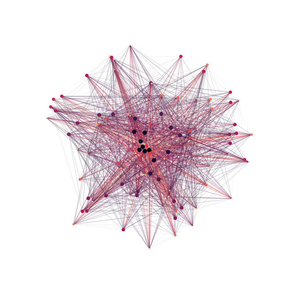
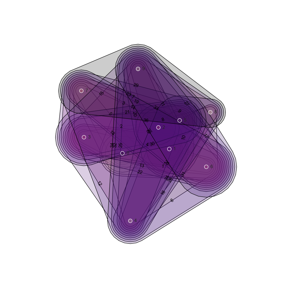
Figure 1. Generated Instances of a 2-layer model with $c=[1.5,2.5],H=[0.25,1],\lambda=\log 3$. Left: $k=2$, Right: $k=3$.

3. Fast Algorithms

Note that the naïve exact computation of the log-likelihood (LL), i.e. without taking into account the sufficient statistics of each hyperedge, requires flipping $\sum_{k=k_{\min}}^{k_{\max}}\binom{n}{k}$ coins in total which is highly prohibitive even for hypergraphs with very small $k_{\max}$ even if $n$ is moderate ($n>100$). In the same way, sampling hypergraphs from CIGAM also needs flipping $\sum_{k=k_{\min}}^{k_{\max}}\binom{n}{k}$ coins which makes sample generation inefficient as well. We also note that in the simple case of graphs with spatial features the work of (Jia and Benson, 2019), the authors approximate the likelihood and sampling of their model, where, in our case, we take advantage of the sufficient statistics of each hyperedge to do exact inference in linear time. Our approach follows the methodology used to sample Kronecker hypergraphs (Eikmeier et al., 2018), however the partitioning of the graph is significantly different in both cases and requires careful calculation.

More specifically, we observe that a graph generated by the CIGAM model can be broken down into multiple Erdös-Rényi graphs, whose block sizes and parameters we devise in Sec. 3.1, and such partitions have efficient representations in terms of the LL as well as can be sampled by standard methods for sampling Erdös-Rényi graphs (Ramani et al., 2019).

3.1. Hyperedge Set Partitioning

From the definition of the model, we deduce that the hyperedge set can be efficiently partitioned, both for sampling and inference, namely each edge in the multi-layer model is determined by $\max_{u\in e}r_{u}$ and $\min_{u\in e}r_{u}$. The edge set $E$ of a hypergraph that contains simplices of order $k\in[k_{\min},k_{\max}]$ is partitioned as

$$E=\bigsqcup_{k\in[k_{\min},k_{\max}],\;i\in[n],\;l\in[L]}E(k,i,l),$$

where $E(k,i,l)=\{e\in E:|e|=k,i=\mathrm{argmax}_{u\in e}r_{u},\phi(e)=l\}$. To sample the multi-layer model, we first assign a layer to each node $i$, assuming again that $r_{1}\succ r_{2}\succ\dots\succ r_{n}$, that is the layer that the current node belongs if its the node with the smallest rank in a given hyperedge. We call this matrix, which has increasing entries, $\texttt{layers[}n\texttt{]}$. We then form $N(i,l)=\{i<j\leq n|\texttt{layers[}j\texttt{]}=l\}$. Now, a hyperedge $e$ needs two components: the largest rank, which determines the exponent of $f(e)$ and the smallest rank in $e$ that determines the layer that the hyperedge is in. We start by iterating on the ranks array and while fixing $i$ as the dominant node: we first select $j$ from $N(i,l)$ and then, we sample $k-2$ nodes from $[i+1,j-1]$, for $j-i-1\geq k-2$ for every $k\in[k_{\min},k_{\max}]$. Therefore, a total of $\sum_{j\in N(i,l)}\binom{j-i-1}{k-2}$ $k$-simplices can belong to the partition where $i$ is the dominant rank node. We construct a $(k_{\max}-k_{\min}-1)\times n\times L$ matrix which contains $|E(k,i,l)|$ for all $k\in[k_{\min},k_{\max}]$, $i\in[n]$ and $l\in[L]$. We iterate over all $e\in E$ and increment the $(|e|,\mathrm{argmax}_{u\in e}\{r_{u}\},\texttt{layers[}\mathrm{argmin}_{u\in e}\{r_{u}\}\texttt{]})$-th entry of the matrix. The complement sets have sizes

$$|\bar{E}(k,i,l)|=\sum_{j\in N(i,l)}\binom{j-i-1}{k-2}-|E(k,i,l)|\quad\forall k,i,l.$$

To simplify the summation, note that by the binomial identity $\binom{j-i-1}{k-2}=\binom{j-i}{k-1}-\binom{j-i-1}{k-1}$, we calculate the sum $\sum_{j\in N(i,l)}\binom{j-i-1}{k-2}$ as

(2) $$\sum_{j\in N(i,l)}\binom{j-i-1}{k-2}=\binom{j_{\max}(i,l)-i}{k-1}-\binom{j_{\min}(i,l)-i-1}{k-1},$$

with $j_{\max}(i,l)=\max_{j\in N(i,l)}j$, and $j_{\min}(i,l)=\min_{j\in N(i,l)}j$ and using the fact that $N(i,l)$ is a contiguous array. We can further validate that for the simple case that $k_{\min}=k_{\max}=k$, $L=1$ we have that $j_{\min}(i,1)=i+1$ and $j_{\max}(i,1)=n$ yielding $|\bar{E}(i,1)|=\binom{n-i}{k-1}-|E(i,1)|$ as expected. As a generative model, each block requires throwing $E|(k,i,l)|$ balls where $|E(k,i,l)|$ follows a binomial r.v. with $\binom{j_{\max}(i,l)-i}{k-1}-\binom{j_{\min}(i,l)-i-1}{k-1}$ trials of bias $c_{l}^{-2+r_{i}}$ for a hyperedge of order $k$. We further simplify the number of trials by noting that $j_{\max}(i,l)=j_{\min}(i,l)+|N(i,l)|-1$ since $N(i,l)$ is a contiguous array. We need $O(k_{\max}(m+n)+n\log n)$ to build the $|E(k,i,l)|$ and time $O(n(k_{\max}+L))$ to build $|\bar{E}(k,i,l)|$ giving a total preprocessing time of $T_{PRE}=O(n(k_{\max}+L)+k_{\max}m+n\log n)$. Usually (see Sec. 5), $k_{\max}$ and $L$ are constant which brings $T_{PRE}$ to $O(n\log n+m)$.

3.2. Exact Inference

Based on the hyperedge set partitioning of Sec. 3.1 we can compute the LL function $\log p(G,r|\lambda,c)$ as follows, assuming the elements of $r$ are sorted in decreasing order:

(3) $$\begin{split}\log p(G,r|\lambda,c)=&-\lambda\sum_{i\in[n]}r_{i}+n\log\lambda-n\log(1-e^{-\lambda})\\ &+\sum_{i,l}\bigg{[}\left(\sum_{k}|E(k,i,l)|\right)\log\left(c_{l}^{-2+r_{i}}\right)\\ &+\left(\sum_{k}|\bar{E}(k,i,l)|\right)\log\left(1-c_{l}^{-2+r_{i}}\right)\bigg{]}.\end{split}$$

Then, the likelihood can be computed in $T_{LL}=O(nL)$ time by precomputing $\sum_{k}|E(k,i,l)|$ and $\sum_{k}|\bar{E}(k,i,l)|$. The total memory required is $O(nL)$ to store $\sum_{k}|E(k,i,l)|$ (resp. $\sum_{k}|\bar{E}(k,i,l)|$), $O(m)$ to store the edges, and $O(nk_{\max})$ to store the binomial coefficients. Therefore, the total memory cost is $O(n(k_{\max}+L)+m)$. Since the number of layers $L$ are constant compared to $n$, the time needed to compute the likelihood is $O(n)$.

The breakpoints $H_{i}$ are hyperparameters of the model. We impose constraints on the density of the edges, i.e. we want the graph to “sparsify” towards the periphery which can be encoded with the following domain $\mathcal{K}=\{(\lambda,c):1<c_{1}<c_{2}\dots<c_{L}\}$. We encode the domain $\mathcal{K}$ on the LL by considering the log-barrier function $\varphi\left(\lambda,c\right)=\log(c_{1}-1)+\sum_{i=1}^{L-1}\log(c_{i+1}-c_{i})$ which equals $-\infty$ for every $(\lambda,c)\notin\mathcal{K}$. Thus, we solve the following inference problem to get the optimal parameters of the model

$$\max_{(\lambda,c)\in\mathcal{K}}\log p(G,r|\lambda,c)\Leftrightarrow\max_{(\lambda,c)\in\mathbb{R}^{L+1}}\log p(G,r|\lambda,c)+\varphi(\lambda,c).$$

3.3. Learning Endogenous Ranks

When the rank vector $r$ is not provided we learn the endogenous (or latent) ranks given a feature matrix $X\in\mathbb{R}^{n\times d}$ by using a learnable model $h(\cdot|\theta)$ to get $r_{i}=h(x_{i}|\theta)$, which we replace on the LL as follows:

$$\begin{split}\log p(G,X|\lambda,c,\theta)&=-\lambda\sum_{i\in[n]}h(x_{i}|\theta)+n\log\lambda-n\log(1-e^{-\lambda})\\ &+\sum_{i,l}\bigg{[}\left(\sum_{k}|E(k,i,l)|\right)\log\left(c_{l}^{-2+h(x_{i}|\theta)}\right)\\ &+\left(\sum_{k}|\bar{E}(k,i,l)|\right)\log\left(1-c_{l}^{-2+h(x_{i}|\theta))}\right)\bigg{]}.\end{split}$$

In Sec. 5, we use a simple logistic model for determining the ranks, i.e. $r_{i}=h(x_{i}|w,b)=\sigma(w^{T}x_{i}+b)$ where $\sigma(\cdot)$ is the sigmoid function. After training, we can use the learned parameters $\theta^{*}$ to extract embeddings that capture the endogenous ranks of nodes in the graph. Besides, we can use centrality measures (degree centrality, [hypergraph] eigenvector centrality for $k$-uniform hypergraphs (Benson, 2019)), PageRank etc.) to enrich the feature vectors. Here, the ranks $r_{i}$ need to be re-sorted after each forward call to $h$ which makes the total per-step cost for evaluating the LL equal to $T_{PRE}+T_{LL}+O(dn)$.

3.4. Choosing Hyperparameters

A question that arises when we fit a multi-layer CIGAM model is the following: How to choose the number of layers $L$ and the breakpoints $H$? We observe that samples generated from CIGAM have roughly a piecewise linear form when the observed degree is plotted versus the degree ordering of a node in the degree ordering in a log-log plot (Fig. 2). This observation motivates the following heuristic for hyperparameter selection: given a hypergraph $G$ we calculate the degrees of all nodes, sort them in decreasing order and fit a piecewise linear function on the log-log scale. We then apply the elbow criterion (Thorndike, 1953) and choose the number of layers to be

$$L_{\mathrm{pw}}=\underset{l\in[2,L_{\max}-1]}{\mathrm{argmax}}\left\{\frac{\log\mathsf{PWFitError}^{*}(l)-\log\mathsf{PWFitError}^{*}(l-1)}{\log\mathsf{PWFitError}^{*}(l+1)-\log\mathsf{PWFitError}^{*}(l)}\right\}$$

where $\mathsf{PWFitError}^{*}(l)$ is the minimum piecewise linear fit error when fitting a function that is a piecewise combination of $l$ lines. Roughly the rule says to pick the number of layers around which the ratio of the subsequent gradients is maximized. Then to identify the breakpoints we run grid search (i.e. likelihood ratio test/AIC/BIC) on all feasible $L_{\mathrm{pw}}$ breakpoints.

3.5. Exact Sampling

Given the parameters $\lambda,c$ of a single-layer model, a reasonable question to ask is: How can we efficiently generate $k$-uniform – and subsequently general hypergraphs – samples from the model with parameters $\lambda,c$? Identically to computing the LL a naiv̈e coin flipping approach is computationally intractable; and can be exponential in the worst case. To mitigate this issue we use the ball-dropping technique to generate edges as follows:

Step 1. Generate the $n$ ranks $r\sim\mathrm{TruncatedExp}(\lambda,[0,1])$ with inverse transform sampling in $O(n)$ time (assuming access to a uniform $[0,1]$-variable in $O(1)$ time). Sort wrt. $\succ$.

Step 2. For each $i\in[n]$ in the order draw a random binomial variable $M_{i}\sim\mathrm{Bin}\left(\binom{n-i}{k-1},c^{-2+r_{i}}\right)$. Drop $M_{i}$ balls, where each ball represents a hyperedge $e$ with $i\in e$ (see App. B for how hyperedges are sampled).

We repeat the same process for various values of $k$ to create a graph with multiple orders. This technique runs much fastetr than $\binom{n}{k}$ (see (Ramani et al., 2019)). The same logic can be extended to the multi-layer model where instead of dropping $M_{i}\sim\mathrm{Bin}\big{(}\binom{n-i}{k-1},c^{-2+r_{i}}\big{)}$ balls for each $i$ on the corresponding spots, we (more generally) throw $M_{i,l}\sim\mathrm{Bin}\left(\binom{j_{\max}(i,l)-i}{k-1}-\binom{j_{\min}(i,l)-i-1}{k-1},c_{l}^{-2+r_{i}}\right)$ for every $i\in[n]$ and $l\in[L]$ where each ball spot is chosen by throwing the first ball between $j_{\min}(i,l)$ and $j_{\max}(i,l)$ and the rest $k-2$ balls between $i$ and $j_{\max}(i,l)$. We again use a rejection sampling mechanism to sample from this space. Finally, to sample a hypergraph with a simplex order range between $k_{\min}$ and $k_{\max}$ we repeat the above process for every $k\in[k_{\min},k_{\max}]$ and take the union of the produced edge sets. Our implementation contains ball-dropping techniques for the general case of multiple layers, however here we present the single layer case for clarity of exposition.

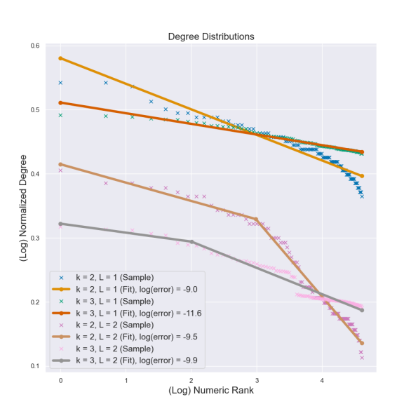
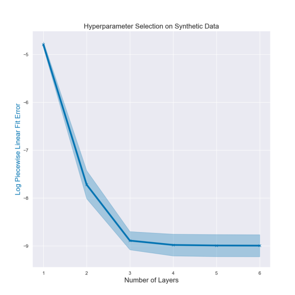
Figure 2. (Left) Degree Plot for an instance with $k\in\{2,3\},L\in\{1,2\}$ layer, $b=3$, $H=1$, $H$ split as powers of $1/2$ in $[0,1]$ and $c$ split uniformly on $[1.5,2.9]$ with p/w fits. (Right) Elbow plot for 10 3-layer simulated graphs.

4. “Small-core” Property

The model we are using serves as a generalization of hierarchical random graph models to random hypergraphs. In those models, see e.g. (Papachristou, 2021), it is often a straightforward calculation to bound the size of the core. Nevertheless, trivially carrying out the same analysis on hypergraphs does not work since the combinatorial structure of the problem changes cardinally, which highlights the needs of new analysis tools in order to be proven.

In detail, in order to characterize the properties of the core of networks generated with CIGAM, we ask the following question: Given a randomly generated $k$-uniform hypergraph $G$ generated by CIGAM, what is the size of its core? In our regime the core is a subset $C$ of the vertices with the following properties:

1. Nodes within the core set $C$ are “tightly” connected with respect to the rest of the graph.

2. Nodes within the core set $C$ form a dominating set for $G$ with high probability (i.e. w.p. $1-O(1/n)$).

For the former requirement, it is easy to observe that the induced subhypergraph that contains nodes with $r_{i}\geq t$ for some appropriately chosen $t$ would form the most densely connected set wrt. the rest of the network. For the latter requirement, we use a probabilistic argument to characterize the core.

Clearly, members of the core are responsible for covering the periphery of the graph, i.e. each peripheral node has at least one hyperedge in the core. Thus the size of the core is the number of nodes that are needed to cover the periphery with high probability. We analyze the core size of the multi-layer model by constructing coupling with a single layer model that generates $k$-uniform hypergraphs with density $c_{L}$ (that corresponds to the “sparsest” density). Then, we start with a threshold $t\in[0,1]$ and we let $N_{k}(t)$ be the number of $(k-1)$-combinations that have at least one rank value $\geq t$. Then, we need to determine the value of $t$ such that (i) $N_{k}(t)$ exceeds some quantity $N_{0}$ with high probability; (ii) the nodes with $r_{j}\geq t$ form an almost dominating set (serving as the core of the graph) with probability $1-O(1/n)$ conditioned on $N_{k}(t)\geq N_{0}$. Proving (ii) proceeds by calculating the (random) probability that a node is not dominated by a core hyperedge, i.e. a hyperedge that has at least one node with $r_{j}\geq t$, and then taking a union bound over the nodes and setting the resulting probability to be at most $1/n$, yielding the desired lower bound $N_{0}$. Now, given that we know $N_{0}$ we want to set it in a value such that $N_{k}(t)\geq N_{0}$ with probability at least $1-1/n$. Observing that $N_{k}(t)$ obeys a combinatorial identity involving $N_{2}(t)$ which is a binomial r.v. and by using the Chernoff bound on $N_{2}(t)$ we can get a high probability guarantee for $N_{k}(t)\geq N_{0}$ by setting $N_{0}$ appropriately. Finally, we set the threshold $t$ such that the probability of having a core at threshold $t$ is at least $1-O(1/n)$. We present the Theorem (proof in App. A)

Theorem 1 (Core Size).

Let $G$ be a $k$-uniform hypergraph on $n\geq 2$ nodes with $k<n$ generated by a CIGAM model with $L$ layers and parameters $1<c_{1}\leq c_{2}\dots\leq c_{L}<e^{\lambda}$ for $\lambda<\tfrac{\ln(n/72)}{4}$. Then, with probability at least $1-2/n$ the graph has a core at a threshold $t$ such that $\tfrac{2\log n}{c_{L}^{-2+t}}=\binom{n}{k-1}-\binom{nF(t)+\sqrt{n\log n/2}}{k-1}$ with size $\widetilde{O}(\sqrt{n})$. $\binom{x}{y}$ is the generalized binomial coefficient.

Fig. 3 depicts the (theoretical) threshold $t$ for a 3-uniform and a 4-uniform hypergraph on 10 nodes. In App. A we also plot the empirical thresholds of CIGAM-generated hypergraphs with $n=200$. As $k$ increases the threshold $t$ moves to the right and therefore the core becomes smaller.

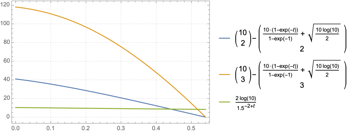
Figure 3. Core threshold functions from Thm. 1 for $c_{L}=1.5,\lambda=1,k\in\{3,4\}$, and $t\in[0,F^{-1}(1-\sqrt{\log n/(2n)})]$ (x-axis).

5. Experiments

We first validate our model’s ability to recover the correct parameters on synthetically generated data, as well as the efficiency of the proposed sampling method. We then perform experiments on small-scale graphs and show that the recovered latent ranks (and their subsequent ordering) can accurately represent the degree structure of the network. Finally, we do experiments with large-scale hypergraph data where we evaluate and compare our model with (generalized) baselines with respect to their abilities to fit the data.

We implement Point Estimation (MLE/MAP) and Bayesian Inference (BI) algorithms as part of the evaluation process, which are available in the code supplement. App. C describes the specifics of each implementation and the design choices, and Tab. 1 shows the costs of fitting CIGAM on various occasions.

Table 1. Time complexity of fitting CIGAM for preprocessing (PP) and log-likelihood (LL). Here $r_{i}=\sigma(w^{T}x_{i}+b)$.

Ranks	Method	# Params	PP	LL
Known	All	$L+1$	$T_{PRE}$	$T_{LL}$
Exogenous	BI	$L+1+n$	–	$T_{PRE}+T_{LL}$
Endogenous	MLE, MAP	$L+d+2$	–	$T_{PRE}+T_{LL}+O(dn)$

5.1. Experiments on Synthetic Data

Sampling. Fig. 4 shows the performance of the ball-dropping method on 2-order and 3-order hypergraphs for graphs with 50-500 nodes with a step of 50 nodes where for each step we sample 10 graphs and present the aggregate statistics (mean and 1 standard deviation).

Inference. In Fig. 4, we generate a 2-Layer graph with $n=100$ nodes, $k\in\{2,3\}$, $\lambda=2.5$, $c=[1.5,2.5]$, $H=[0.5,1]$, and use non-informative priors for recovery. Our algorithm can successfully recover the synthetic data.

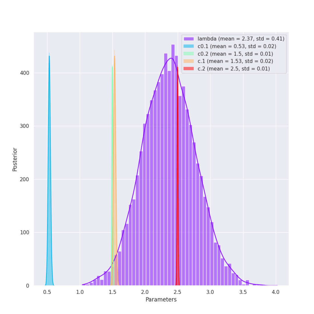
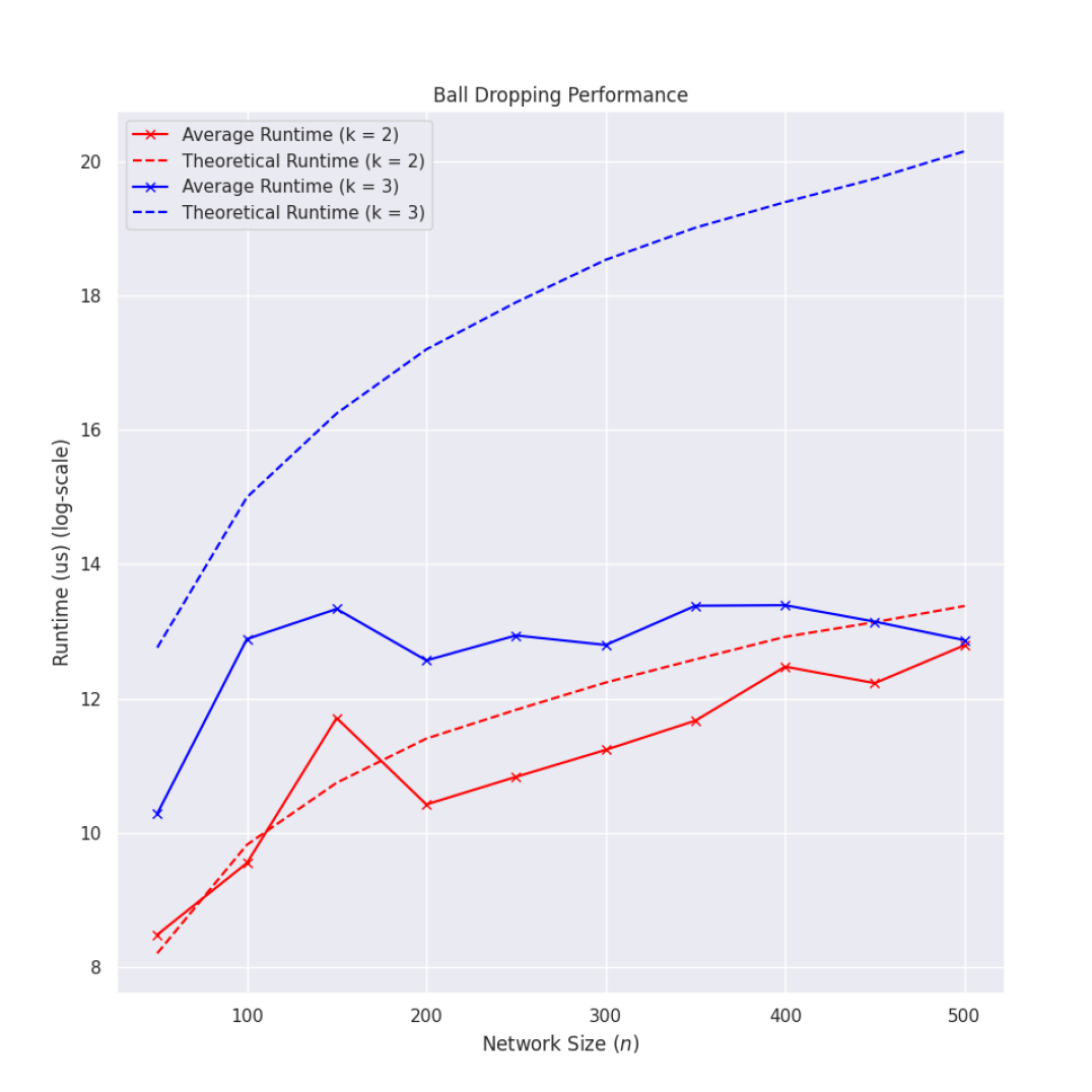
Figure 4. (Top) Parameter recovery for $n=100,k\in\{2,3\},c=[1.5,2.5],\lambda=2.5$. Legend: c0 corresponds to off-by-one parameters and c corresponds to the actual parameters. (Bottom) Average Runtime of Sampling Using the Ball Dropping Method for hypergraphs of orders $k\in\{2,3\}$ and $50-500$ nodes with a step of 50 nodes for an 1-layer instance with $b=3,c=1.5$. The dashed line is the function is the expected number of edges of a $k$-uniform CIGAM hypergraph.

5.2. Recovering the Degree Structure of small-scale graphs

We perform BI on world-trade, c-elegans, history-faculty, and business-faculty using $L=1$ layer, a $\mathrm{Gamma}(2,2)$ prior for $\lambda$, and a $\mathrm{Pareto}(1,2)$ prior for $c$. In Fig. 5, we order the actual degrees of the graphs in decreasing order and for every draw of the vector $r$ from the posterior (using MCMC with $N=1\text{K}$ samples) as follows: (i) We sort the entries of $r$ in decreasing order. Let $\{\pi\}_{i\in[N]}$ be the corresponding permutations of the nodes. For each $i\in[n]$ we calculate the mean and the standard deviation of $\begin{pmatrix}\texttt{degrees[}\pi_{1,i}\texttt{]},\dots,\texttt{degrees[}\pi_{N,i}\texttt{]}\end{pmatrix}^{T}$. The scales of Fig. 5 are log-log. We observe that the degrees as they are determined by the ranks are consistent with the actual degree sequence. This suggests that core-periphery organization agrees with the degree centralities, as in (Papachristou, 2021).

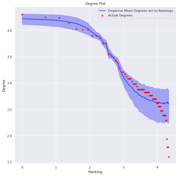
(a) world-trade (De Nooy et al., 2018) ($n=76,m=845$)

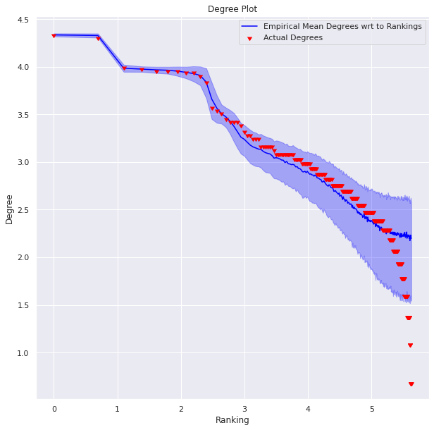
(b) c-elegans (Kaiser and Hilgetag, 2006) ($n\!=\!279,m\!=\!1.9\mathrm{K})$

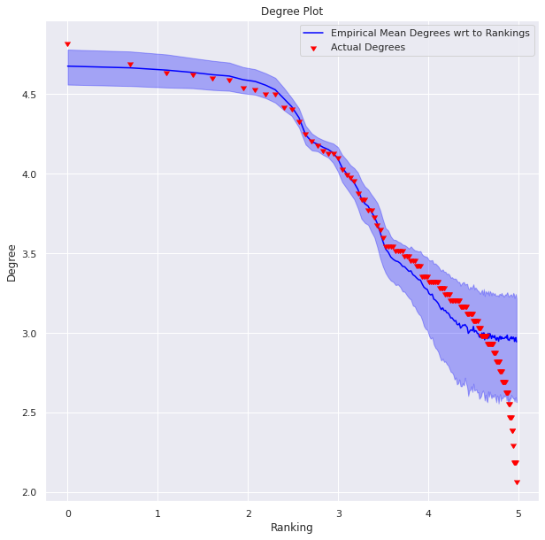
(c) history (Clauset et al., 2015) ($n\!=\!145,m\!=\!2\mathrm{K}$)

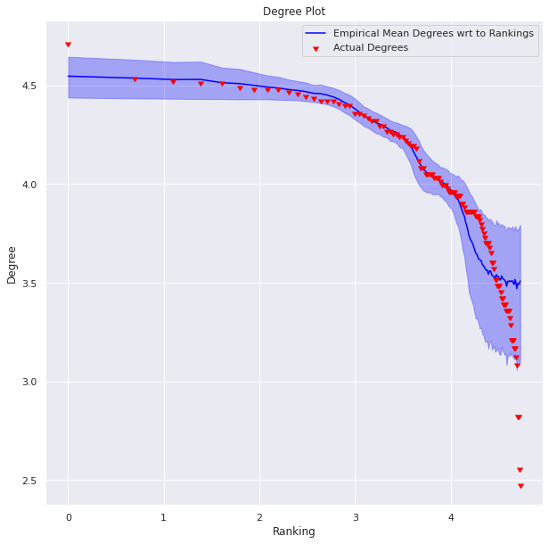
(d) business (Clauset et al., 2015) ($n\!=\!113,m\!=\!3\mathrm{K})$

Figure 5. Recovery of the Degree Structure for world-trade, c-elegans, history-faculty, and business-faculty datasets.

5.3. Experiments with large-scale data

Datasets. We perform experiments with publicly available datasets.

Table 2. Dataset Statistics. $n_{LCC},m_{LCC}$ refer to the size of the LCCs, $n_{dt},m_{dt}$ refers to the size of the LCCs after removing nodes with degree $\leq 4$, $n_{kc},m_{kc}$ refers to the size of the 2-core of the LCC.

Dataset	$k_{\max}$	$n_{LCC}$	$m_{LCC}$	$n_{dt}$	$m_{dt}$	$n_{kc}$	$m_{kc}$
c-MAG-KDD	22	2.7K	1.4K	47	40	–	–
t-ask-ubuntu	6	6.2K	7.8K	664	1.7K	50	33
t-math-sx	7	26.4K	66.1K	5.4K	39.2K	100	58
t-stack-overflow	10	164.9K	306.4K	34.3K	140.4K	7.0K	6.0K
ghtorrent-p	7	78.4K	74.8K	10.8K	14.8K	3.4K	2.7K

Table 3. Hypergraph Experiments. We use SGD with step-size 0.001 for CIGAM, and SGD with stepsize of 1e-6 for Logistic-CP, for 10 epochs. For HyperNSM we use $a=10$, $p=20$, and $\xi(e)=1/|e|$. For evaluating the log-likelihood of Logistic-CP and HyperNSM we use $|\mathcal{B}|=0.2\bar{m}$ negative samples. Best likelihood is in bold. † = LL cannot be computed.

Dataset	CIGAM	$c^{*}$	$\lambda^{*}$	Logistic-CP	HyperNSM	CIGAM	$c^{*}$	$\lambda^{*}$	Logistic-CP	HyperNSM
	Degree Threshold + LCC					LCC + 2-core
	Exogenous ranks
coauth-MAG-KDD	-1334	[3.0e+4]	1.4	-2025	-2.5e+6	–	–	–	–	–
threads-ask-ubuntu	-1.3e+5	[9.5e+9]	3.5	†	†	-166	[11.94]	1.5	-1510	-1073
threads-math-sx	-4.2e+6	[2.3e+20]	8.7	†	†	-1736	[5.2, 31.1]	1.8	-1478	-1.4e+5
threads-stack-overflow	-2.0e+7	[1.8e+20, 8.3e+27]	4.8	†	†	-1.2e+5	[2.1e+5]	5.1	-1.0+e7	†
ghtorrent-projects	-1.2e+6	[7.8e+15, 5.9e+20]	4.4	†	†	-2.6e+5	[9.4e+18]	3.6	†	†
	Endogenous (Learnable) ranks
coauth-MAG-KDD	-1.8e+5	[32.4]	1.1	-2024	-2.5e+6	–	–	–	–	–
threads-ask-ubuntu	-1.6e+5	[9.6e+6]	1.1	†	†	-2079	[1.1]	1.1	-1659	-1075
threads-math-sx	-4.2e+6	[2.3e+20]	11.3	†	†	-3.8e+4	[2.8]	1.1	-5.8e+4	-1.4e+5
threads-stack-overflow	-1.9e+7	[4.1e+29]	26.8	†	†	-4.0e+5	[8.6e+8]	1.1	†	†
ghtorrent-projects	-1.2e+6	[2.9e+22]	2.8	†	†	-2.1e+5	[9.4e+20]	1.1	†	†

1. coauth-MAG-KDD. Contains all papers published at the KDD conference and are included in the Microsoft Academic Graph v2 (Tang et al., 2008; Sinha et al., 2015). We also include data for each of the authors’ number of citations, h-index, number of publications and use the R package amelia (Honaker et al., 2011) to impute missing data at rows where at least one of the columns exists after applying a log-transformation.

2. ghtorrent-projects. We mined timestamped data from the ghtorrent project (Gousios and Spinellis, 2012; Gousios, 2013) and created the ghtorrent-projects dataset where each hyperedge corresponds to the users that have push access to a repository. We used features regarding: number of followers on GitHub, number of commits, number of issues opened, number of repositories created, and the number of organizations the user participates at.

3. threads-{ask-ubuntu, math-sx, stack-overflow} (Benson et al., 2018). Nodes are users on askubuntu.com, math.stackexchange.com, and stackoverflow.com. A simplex describes users participating in a thread that lasts $\leq 24$ hours. We observe that there is a high concentration of (non-engaged) users with reputation 1 and then the next peak in the reputation distrubution is at reputation 101. This bimodality is explained since Stack Exchange gives users an engagement bonus of 100 for staying on the platform. Therefore, we filter out all the threads at which non-engaged users (i.e. users with reputation less than 101) participate. We keep the (platform-given) reputation (as the ranks), the up-votes, and the down-votes of each user as her features.

Deduplication. We keep each appearing hyperedge exactly once.

Outlier Removal & Feature Pre-processing. We filter outliers from the data in two ways. This is done in order to guarantee the numerical stability of the fitting algorithms. In the former filtering (Degree Threshold + LCC), we remove all nodes with degree $<4$ and then find the Largest Connected Component (LCC) of the resulting data. In the latter filtering (LCC + 2-core) we first find the LCC of the hypergraph and then keep the 2-core within it. The statistics of the post-processed datasets can be found at Tab. 2.

In the experiments considering exogenous ranks only, we take logarithms (plus one) of the exogenous ranks and min-max normalize the results to lie in $[0,1]$. For the learning task (i.e. endogenous ranks), we perform standard $Z$-normalization (i.e. subtract column means and divide by the column stds.) in lieu of min-max normalization.

Table 4. Projected Graph Experiments. We use SGD with step-size 0.001 for CIGAM, and SGD with stepsize of 1e-6 for Logistic-CP, for 10 epochs. For evaluating the log-likelihood of Logistic-CP, and Logistic-TH $(\alpha=10,p=20)$ we use $|\mathcal{B}|=0.2\bar{m}$ negative samples. Best likelihood in bold. † = LL cannot be computed.

Dataset	CIGAM	$c^{*}$	$\lambda^{*}$	Logistic-CP	Logistic-TH	CIGAM	$c^{*}$	$\lambda^{*}$	Logistic-CP	Logistic-TH
	Degree Threshold + LCC					LCC + 2-core
	Exogenous ranks
coauth-MAG-KDD	-532	[12.2]	1.4	-1532	-1419	–	–	–	–	–
threads-ask-ubuntu	-2.8e+4	[1.9e+3]	3.5	-1.3e+4	-2.4e+5	-166	[11.94]	1.5	-1510	-1329
threads-math-sx	-8.5e+5	[116.1, 2.0e+3]	8.7	-6.1e+6	-1.6e+7	-564	[2.7, 4.9]	1.8	-1376	-5471
threads-stack-overflow	-4.0e+6	[5.1e+6]	4.8	†	†	-1.2e+5	[2.1e+5]	5.1	†	-2.7e+7
ghrtorrent-projects	-4.9e+6	[1.7e+6]	4.4	†	†	-7.4e+5	[359.3, 951.3]	3.6	†	-1.8e+6
	Endogenous (Learnable) ranks
coauth-MAG-KDD	-2171	[1.1]	1.1	-1680	-1458	–	–	–	–	–
threads-ask-ubuntu	-5.0e+4	[3.2]	1.1	-3.4e+4	-2.8e+5	-185	[12.1]	1.3	-1666	-1329
threads-math-sx	-1.3e+6	[1.2e+5]	10.7	†	†	-402	[45.2]	1.7	-1926	-5471
threads-stack-overflow	-3.8e+6	[5.2e+6]	20.7	†	†	-1.2e+5	[2.1e+5]	1.9	-1.0e+7	-2.7e+7
ghtorrent-projects	-7.1e+5	[5.1e+5]	4.4	†	†	-5.7e+4	[1.4e+4]	4.5	-1.9e+5	-1.8e+6

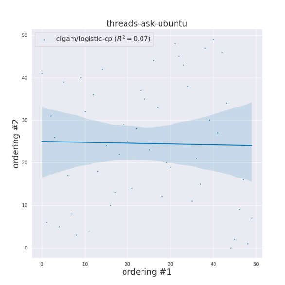
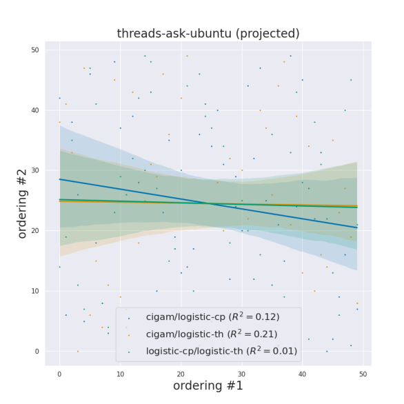
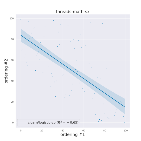
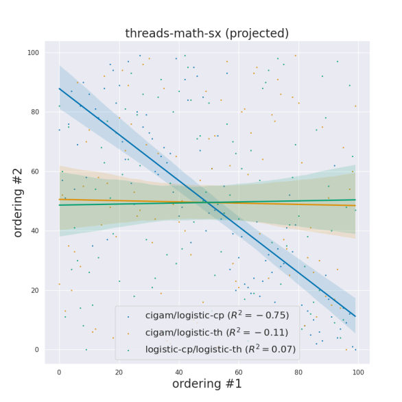
Figure 6. Ranking comparison between algorithms (Tabs. 3, 4) for threads-{ask-ubuntu, math-sx} datasets (LCC + 2-core).

Hypergraph Experiments. We compare CIGAM with the baseline (without spatial dependencies) logistic model of (Jia and Benson, 2019). This model is also known as the $\beta$-model (Stasi et al., 2014; Wahlström et al., 2016) and has been already generalized to hypergraphs (see (Stasi et al., 2014)). However, the inference algorithm of (Stasi et al., 2014) suffers from combinatorial explosion since for every node, the fixed-point equations require a summation over $\binom{n-1}{k-1}$ terms for a $k$-uniform hypergraph which makes the inference task infeasible for the datasets we study.

Logistic-CP generates independent hyperedges based on the sum of core scores $\sum_{i\in e}z_{i}$ for a hyperedge $e$, i.e. $e$ is generated with probability $\rho(e)=\sigma\left(\sum_{i\in e}z_{i}\right)$ where $\sigma(z)=\tfrac{1}{1+e^{-z}}$. That corresponds to a LL $\log p(G|z)=\sum_{e\in E}\log\rho(e)+\sum_{\bar{e}\notin E}\log(1-\rho(e))$. In contrast to our model, computing the likelihood of Logistic-CP and its gradient exactly is – contrary to the case of CIGAM – intractable since it requires exhaustively summing over $\bar{e}\notin E$ which can be very large. To approximate the log-likelihood we use negative sampling by selecting a batch $\mathcal{B}$ as follows: We sample a hyperedge order $K\in[k_{\min},k_{\max}]$ with probability $\Pr[K=k]=\tfrac{\bar{m}_{k}}{\bar{m}}$ where $\bar{m}_{k}=\binom{n}{k}-m_{k}$ denotes the number of negative hyperedges of order $k$ and then given the sampled order $K$ we sample a negative hyperedge $\bar{e}$ uniformly from the set of non-edges of order $k$. That uniform sampling scheme has a probability of selecting a hyperedge $\bar{e}$ equal to $\tfrac{|\mathcal{B}|}{\bar{m}}$ (App. B describes the sampling algorithm). We use the following unbiased estimator of the LL based on this sampling scheme,

(4) $$\hat{\ell}(G|z)=\sum_{e\in E}\log\rho(e)+\frac{\bar{m}}{|\mathcal{B}|}\sum_{\bar{e}\sim\mathcal{B}}\log(1-\rho(\bar{e})),$$

where its easy to confirm that $\mathbb{E}\left[\hat{\ell}\right]=\log p(G|\theta)$, and that $\mathrm{Var}\left[\hat{\ell}\right]=\frac{\bar{m}-|\mathcal{B}|}{|\mathcal{B}|}\sum_{\bar{e}\in\bar{E}}\log^{2}(1-\rho(\bar{e}))$, which is at most $\tfrac{(\bar{m}-|\mathcal{B}|)\bar{m}}{|\mathcal{B}|}$ for $\rho(\bar{e})\in[0,0.51]$ (true for real-world datasets). Letting $|\mathcal{B}|=\alpha\bar{m}$ for some $\alpha\in(0,1)$ we get a variance upper bound that equals $\tfrac{1-\alpha}{\alpha}\bar{m}$ for small values of $\rho(\bar{e})$. The per-step complexity of approximately computing the likelihood and its gradient in this case is both higher than computing the LL for CIGAM. Logistic-CP can also be augmented with the use of features and a learnable map $\psi$ with parameters $\nu$ such that $z_{i}=\psi(x_{i}|\nu)$. In this model, the core nodes are nodes with $z_{i}\geq 0$ and the periphery nodes are nodes with $z_{i}<0$ respectively.

We also use the concurrent and independently developed method of (Tudisco and Higham, 2022) – HyperNSM – where a permutation $\pi$ of the nodes is generated and then hyperedges are independently generated with probability $\sigma\left(\xi(e)M_{a}(\{a_{u}\}_{u\in e})\right)$, where $M_{a}$ denotes the generalized (Hölder) $a$-mean. $\xi(e)$ is a weight function (e.g. $\xi(e)=1/|e|$) and $a_{u}=1-\tfrac{\pi_{u}}{n}$. The goal of HyperNSM is to recover the optimal permutation $\pi^{*}$ of the nodes through a fixed-point iteration scheme. To calculate the LL of HyperNSM we use negative sampling such as in the case of Logistic-CP.

Tab. 3 shows the results of comparing CIGAM with Logistic-CP, and HyperNSM. As in Section 4.2 of (Jia and Benson, 2019), we compare the optimized LL values of both CIGAM, Logistic-CP, and HyperNSM. We run experiments both using exogenous ranks (directly from the features), as well as endogenous (learnable) ranks via the mined features. We also report the learned core profile $c^{*}$ and the learned $\lambda^{*}$ for all datasets. The breakpoints are taken with step $0.5$. In almost all of the experiments, CIGAM has a substantially better optimal LL than its competitors, which in many cases cannot scale (because GPUs run out of memory) to even moderate dataset sizes (denoted by ${\dagger}$). In terms of learned parameters, we observe that most of the datasets are very sparse (very high values of $c^{*}$) in both the exogenous and the endogenous case. In App. D, we show how to add regularization (or priors) to the model.

Projected Hypergraph Experiments. We run the same experiments as in Tab. 3 but instead of the hypergraph data, we use the projected graphs that result from replacing each hyperedge with a clique. We also use the model of (Tudisco and Higham, 2019b), together with Logistic-CP and CIGAM. More specifically, the model of (Tudisco and Higham, 2019b), which we call Logistic-TH, is a logistic-based model (the graph analogue of HyperNSM) that depends on finding a permutation $\pi$ of the nodes. In this model, and edge $(u,v)$ is generated independently with probability $\sigma(M_{a}(a_{u},a_{v}))$ where $a_{u}=1-\frac{\pi_{u}}{n}$ (resp. $a_{v}$). The authors devise an iterative method to optimize the LL of the corresponding generative model. The iterative method converges to a fixed point vector $x^{*}$, and the ordering of the elements of $x^{*}$ implies the optimal permutation $\pi^{*}$. Again, to calculate the LL after finding $\pi^{*}$ we use negative sampling.

We report the experimental results in Tab. 4. Again, we observe that CIGAM is able to find better fits than both Logistic-CP and Logistic-TH, while it is also able to scale more smoothly to the largest datasets. Furthermore, we observe that the values of $c^{*}$ that CIGAM finds compared to the hypergraph case are substantially smaller. This can be attributed to the fact that the projected hypergraphs have a smaller possible number of edges (i.e. $\binom{n}{2}$), and, thus, they are “denser” than the hypergraph instances since hyperedges are projected on the same order.

Ranking Comparison. In Fig. 6 we compare the node orderings produced by CIGAM and Logistic-CP (and Logistic-TH in the graph case) on threads-ask-ubuntu and threads-math-sx (LCC + 2-core). We observe that in threads-ask-ubuntu have uncorrelated rankings, whereas in the case of threads-math-sx the rankings are negatively correlated. So, in both cases, the two algorithms are producing different rankings. Finally, we observe that both Logistic-CP and CIGAM are uncorrelated with the rankings that Logistic-TH produces. This is indicative of the algorithms having a different way on ranking the nodes. Indeed, Logistic-CP creates edges based on the sum of the core scores of the nodes, CIGAM creates edges based on the nodes with the maximum and minimum ranks, while Logistic-TH uses the generalized mean to resolve a version of the problem in the spectrum “between” CIGAM and Logistic-CP.

Applications & Future Work. Similarly to graphs (see e.g. (Papachristou, 2021)), hypergraphs with a small core can be utilized to speed up computational tasks ( community detection, clustering, embeddings, user modeling, fandom formation etc.) that can be performed within the sublinear core and then the results can be aggregated to the periphery.

Finally, it should be noted that CIGAM does not have control over motifs, and the experimental or theoretical study of the distributions of motifs is interesting future work.

Acknowledgements. Supported in part by a Simons Investigator Award, a Vannevar Bush Faculty Fellowship, AFOSR grant FA9550-19-1-0183, a Simons Collaboration grant, and a grant from the MacArthur Foundation.The authors would like to thank A. Benson, E. Pierson, A. Singh, K. Tomlinson, J. Ugander, and Y. Wang for the useful discussions.

Appendix A Core Structure

A.1. Proof of Theorem 1

Coupling construction. Let a CIGAM model $G_{1}$ with parameters $\lambda$ and $1<c_{1}\leq c_{2}\dots\leq c_{L}<e^{\lambda}$ be given and let a CIGAM model $G_{2}$ have parameters $\lambda$ and one layer with value $c_{L}$. We construct the coupling $\nu$ as follows: We first sample the rank vector $r$ (common for both $G_{1}$ and $G_{2}$) and then construct the hyperedges as follows: (i) If a hyperedge appears on $G_{2}$ then with probability 1 is appears on $G_{1}$, and (ii) if a hyperedge does does not appear on $G_{2}$ then it appears on $G_{1}$ with probability $\frac{f_{1}(e)-f_{2}(e)}{1-f_{2}(e)}$. We can easily show that the marginals satisfy $\Pr[e\in E(G_{1})|r]=f_{2}(e)\cdot 1+(1-f_{2}(e))\frac{f_{1}(e)-f_{2}(e)}{1-f_{2}(e)}=f_{1}(e)$ and $\Pr[e\in E(G_{2})|r]=f_{2}(e)$. Finally, we integrate over $r$ to get that $\Pr[e\in E(G_{1})]=f_{1}(e)$ and $\Pr[e\in E(G_{2})]=f_{2}(e)$. Therefore $\nu$ is a valid coupling. Under $\nu$ we have that always $G_{2}\subseteq G_{1}$. Therefore, it suffices to prove the Theorem for $G_{2}$ to get a result that holds for $G_{1}$.

Core size. We prove the statement in the case that $G_{1}$ is $k$-uniform. Since by the coupling construction $G_{2}\subseteq G_{1}$, proving a statement for the size of the core on $G_{2}$ will also hold for $G_{1}$ since a dominating set in $G_{2}$ is a dominating set in $G_{1}$. Let $t\in[0,1]$ be a threshold value to be determined later. Define

$$N_{k}(t)=\sum_{(j_{1},\dots j_{k-1})\in\binom{[n]}{k-1}}\bm{1}\{\max\{r(j_{1}),\\ \dots,r(j_{k-1})\}\geq t\}$$

be the number of nodes with ranks at least $t$. Note that by a simple combinatorial argument

$$\begin{split}N_{k}(t)&=\binom{n}{k-1}-\left|J\in\binom{[n]}{k-1}:\forall j\in J,r_{j}<t\right|\\ &=\binom{n}{k-1}-\binom{n-N_{2}(t)}{k-1}\end{split}$$

where $N_{2}(t)\sim\mathrm{Bin}(n,1-F(t))$ is the number of nodes with $r_{j}\geq t$ and $\binom{x}{y}=\frac{\Gamma(x+1)}{\Gamma(y+1)\Gamma(x-y+1)}$ is the generalized biniomial coefficient. The function $g(\nu)=\binom{n}{k-1}-\binom{n-\nu}{k-1}$ is strictly increasing for $0\leq\nu\leq n$. Therefore, we can directly devise a concentration bound for $N_{k}(t)$ via concentration bounds for $N_{2}(t)$. Indeed, by the Chernoff bound

$$\Pr\bigg{[}N_{k}(t)\geq\binom{n}{k-1}-\binom{n-\mathbb{E}\left[N_{2}(t)\right]+\sqrt{n\log n/2}}{k-1}\bigg{]}$$

$$=\Pr[N_{2}(t)\geq\mathbb{E}\left[N_{2}(t)\right]-\sqrt{n\log n/2}]\geq 1-\frac{1}{n}$$

as long as $t\leq F^{-1}(1-\sqrt{\log n/(2n)})$. Note that the probability that a node $i\in[n]$ is not dominated by any core-hyperedge is given by

$$\Pr[\text{$i$ is not dominated by the core}]$$

$$=\prod_{J\in\binom{[n]}{k-1}}\left(1-c_{L}^{-2+\max_{j\in J\cup\{i\}}r_{j}}\right)^{\bm{1}\{\max_{j\in J}r_{j}\geq t\}}$$

$$\leq\prod_{J\in\binom{[n]}{k-1}}\left(1-c_{L}^{-2+t}\right)^{\bm{1}\{\max_{j\in J}r_{j}\geq t\}}$$

$$=\left(1-c_{L}^{-2+t}\right)^{N_{k}(t)}\leq\exp(-N_{k}(t)c_{L}^{-2+t}).$$

If $N_{k}(t)\geq\frac{2\log n}{c_{L}^{-2+t}}$ then by the union bound $\Pr[\exists i:\text{$i$ is not}\\ \text{dominated by the core}|N_{k}(t)\geq 2\log n/c_{L}^{-2+t}]\leq\frac{1}{n}$. Subsequently, the complementary event (i.e. $\forall i$, $i$ is dominated by the core) happens with probability at least $1-1/n$. We let $t$ to be such that

(5) $$\frac{2\log n}{c_{L}^{-2+t}}=\binom{n}{k-1}-\binom{nF(t)+\sqrt{n\log n/2}}{k-1},$$

in order for $\Pr[N_{k}(t)\geq 2\log n/c_{L}^{-2+t}]\geq 1-\tfrac{1}{n}$. Finally we have that given $t$ that satisfies (5)

$$\Pr\left[\text{Core at threshold $t$}\right] \geq\left(1-\frac{1}{n}\right)^{2}\geq 1-\frac{2}{n}.$$

Existence and Uniqueness of threshold $t$. We define

(6) $$\Phi(t)=\frac{2\log n}{c_{L}^{-2+t}}-\binom{n}{k-1}+\binom{nF(t)+\sqrt{n\log n/2}}{k-1}$$

in the range $[0,t^{\prime}]$ where $t^{\prime}=F^{-1}\left(1-\sqrt{\frac{\log n}{2n}}\right)$ is the point where the difference of the binomial coefficients becomes 0. Note that $\Phi$ is continuous and differentiable in $[0,t^{\prime}]$ with derivative

$$\Phi^{\prime}(t) =-2\log c_{L}\log n/c_{L}^{-2+t}+\binom{nF(t)+\sqrt{n\log n/2}}{k-1}nf(t)\psi(nF(t)$$

$$+\sqrt{n\log n/2})$$

$$\geq-2e^{2\lambda}\lambda e^{-\lambda t}\log n+\binom{nF(t)+\sqrt{n\log n/2}}{k-1}nf(t)\psi(nF(t)$$

$$+\sqrt{n\log n/2})$$

$$\geq nf(t)\left[-2e^{2\lambda}+\binom{nF(t)+\sqrt{n\log n/2}}{k-1}\psi(nF(t)+\sqrt{n\log n/2})\right]$$

$$\geq nf(t)\left[-2e^{2\lambda}+\binom{\sqrt{n\log n/2}}{k-1}\psi(\sqrt{n\log n/2})\right]$$

$$\geq nf(t)\left[-2e^{2\lambda}+\sqrt{n\log n/2}\psi(\sqrt{n\log n/2})\right]$$

$$\geq nf(t)\left[-2e^{2\lambda}+\sqrt{n\log n/2}\left[\frac{1}{2}\log(n\log n/2)-\frac{1}{\sqrt{n\log n/2}}\right]\right]$$

$$\geq nf(t)\left[-3e^{2\lambda}+\sqrt{n/8}\right]>0.$$

for $\lambda<\frac{\ln(n/72)}{4}\in o(\log n)$. $\psi(x)=\frac{\Gamma^{\prime}(x)}{\Gamma(x)}$ is the digamma function. For the inequalities we have used the facts: (i) $c_{L}<e^{\lambda}$, (ii) $\log n\leq n$, (iii) monotonicity of the Gamma and the digamma function for $t\geq 0$, (iv) $\binom{n}{k-1}\geq n$ for $k<n-1$, (v) $\psi(x)\geq\log x-\frac{1}{x}$, (vi) $n\geq 2$. Therefore $\Phi(t)$ is strictly increasing. Note that $\Phi(0)=2c_{L}^{2}\log n-\binom{n}{k-1}+\binom{\sqrt{n\log n}}{k-1}<0$ for large enough $n$ and since $c_{L}=o(n)$. Moreover note that $\Phi(t^{\prime})=2\log n/c_{L}^{-2+t^{\prime}}>0$. Therefore $\Phi(0)\Phi(t^{\prime})<0$. Thus by Bolzano’s theorem and the fact that $\Phi^{\prime}(t)>0$ we get that there exists a unique threshold $t\in[0,t^{\prime}]$ such that $\Phi(t)=0$.

Upper Bound. Note that the threshold is maximized when $k=2$, i.e. in the graph case, and therefore the expected size of the core satisfies $\mathbb{E}\left[\text{Core size}\right]\leq n(1-F(t(k=2)))=\sqrt{n\log n/2}+2\log n/c_{L}^{-2+t}=\widetilde{O}(\sqrt{n})$ (see also Fig. 3).

A.2. Empirical Core Thresholds

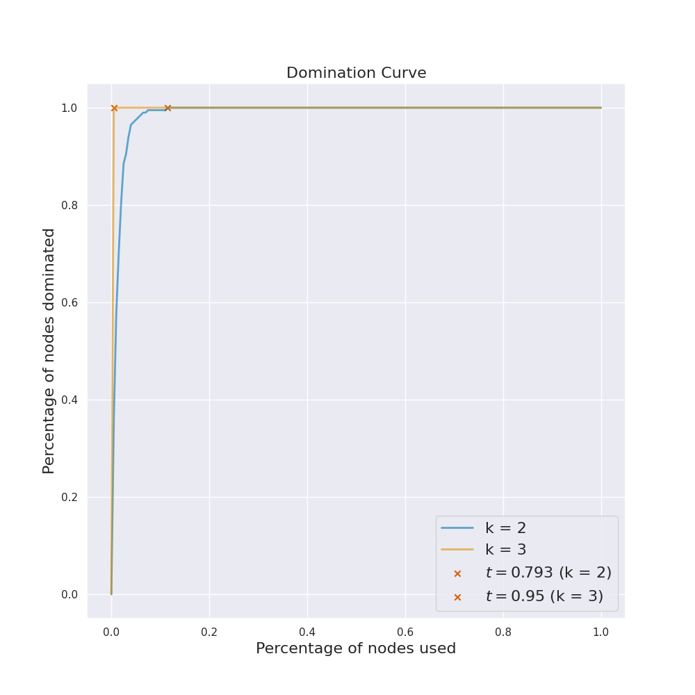
Figure 7. Empirical core Threshold on generated instances for single layer model with $n=200$, $b=3.5$, $c_{1}=3$ for $k\in\{2,3\}$. By ‘‘x’’ we denote the sample core threshold values.

Appendix B Sampling

Uniformly Sampling from $\binom{[n]}{k}$. To sample a $k$-tuple uniformly at random we use a rejection sampling algorithm:

1. Initialize $S\leftarrow\emptyset$.

2. While $|S|\leq k$ repeat: Sample $i$ uniformly from $[n]$, and if $i\notin S$, add $i$ to $S$.

Ball-dropping (Single-Layer / $k$-uniform). For each $i\in[n]$ we create a set $\mathcal{B}_{i}$ in which we sample $M_{i}$ edges by sampling an edge $e$ uniformly from $\binom{[n]}{k-1}$ (with $i$ being the dominant node, and if $e\cup\{i\}$ does not belong to $\mathcal{B}_{i}$ we add it to $\mathcal{B}_{i}$.

Sampling Negative Edges. To sample edges from $e\in\bar{E}$ (i.e. $e\notin E$) we maintain a set $\mathcal{B}$ of certain size $b$ and while $|\mathcal{B}|\leq b$ we sample uniformly an order $\{K=k\}$ with probability $\frac{\bar{m}_{k}}{\bar{m}}$ and then we sample $\bar{e}$ from $\binom{[n]}{k}$ uniformly. If $\bar{e}\notin(E\cup\mathcal{B})$ then we update $\mathcal{B}\leftarrow\mathcal{B}\cup\{\bar{e}\}$.

Appendix C Implementations

Methods. We implement point estimation and Bayesian inference algorithms as part of the evaluation process, which are available in the code supplement. Tab. 1 shows the costs of fitting CIGAM on various occasions.

1. Point Estimation (MLE/MAP). We implement point estimation for the parameters $(\lambda,c)$ (or $(\lambda,c,\theta)$) of CIGAM with PyTorch using the log-barrier method. We use Stochastic Gradient Descent (SGD) to train the model for a certain number of epochs, until the learned parameters have converged to their final values. To avoid underflows, and because the resulting probabilities at each epoch are $\ll 1$ we use a smoothing parameter $\gamma$ (here we use $\gamma=10^{-10}$). which we add to the corresponding probabilities to avert underflow. For MAP we add priors/regularization to $\lambda,c$ (see App. D). For Logistic-CP we use the following architecture to learn $z_{i}$’s: Linear($d$, $d$) $\to$ ReLU $\to$ Linear($d$, $1$).

2. Bayesian Inference (BI). We implement the posterior sampling procedures with mc-stan (Gelman et al., 2015) which offers highly efficient sampling using Hamiltonian Monte Carlo with No-U-Turn-Sampling (HMC-NUTS) (Hoffman et al., 2014) and compiles a C++ model for BI. Note that $\mathcal{K}$ is a convex polytope. Finally, we add priors (see App. D) on the parameters to form a posterior density to sample from. For BI, the stan model samples from the truncated density via defining the parameter c0 as a positive_ordered vector (which induces a log-barrier constraint on the log-posterior) and the parameter c is devised as c0 + 1 in the transformed parameters block. The preprocessing takes place in the transformed data block, and the model block is responsible for the log-posterior oracle.

Tab. 1 shows the complexity of the implemented methods.

Table 5. Experiments with Regularization $\alpha_{c}=100,\alpha_{\lambda}=1,\beta_{\lambda}=2$ (LCC + 2-core) for the StackExchange datasets for SGD with step-size 0.001 and 10 epochs.

Dataset	$c^{*}$	$\lambda^{*}$	$c^{*}$	$\lambda^{*}$
	Hypergraph		Projected
threads-ask-ubuntu	[11.1]	1.3	[11.1]	1.3
threads-math-sx	[1522]	1.9	[44.1]	1.7
threads-stack-overflow	[8.6e+11]	10.5	[2.1e+5]	10.9

Appendix D Priors & Regularization

For notational convenience, we refer to the priors using the variables defined in the stan model. For CIGAM we can use exponential priors for c (or c0 respectively), i.e. we can impose a penalty of the form $p(\texttt{c0})\propto e^{-\alpha_{c}\sum_{i\in[L]}\texttt{c0}_{i}}$. Moreover, a stronger penalty can be applied in terms of a Pareto prior, i.e. $p(\texttt{c})\propto e^{-\alpha_{c}\sum_{i\in[L]}\log(\texttt{c}_{i})}$. For the rank parameter $\lambda$ we impose a $\texttt{Gamma}(\alpha_{\lambda},\beta_{\lambda})$ prior.

For Logistic-CP we can use L2 regularization for $z_{i}$ which corresponds to a Gaussian prior $p(z)\propto e^{-\frac{\alpha_{\theta}}{2}\sum_{i\in[n]}z_{i}^{2}}$ to penalize large values of the core scores both in terms of core ($z_{i}\geq 0$) and periphery ($z_{i}<0$) nodes.

Tab. 5 shows the learned parameters when regularization is applied.

References

- (1)
- Amburg et al. (2021) Ilya Amburg, Jon Kleinberg, and Austin R Benson. 2021. Planted hitting set recovery in hypergraphs. Journal of Physics: Complexity 2, 3 (2021), 035004.
- Benson (2019) Austin R Benson. 2019. Three hypergraph eigenvector centralities. SIAM Journal on Mathematics of Data Science 1, 2 (2019), 293–312.
- Benson et al. (2018) Austin R Benson, Rediet Abebe, Michael T Schaub, Ali Jadbabaie, and Jon Kleinberg. 2018. Simplicial closure and higher-order link prediction. Proceedings of the National Academy of Sciences 115, 48 (2018), E11221–E11230.
- Benson and Kleinberg (2018) Austin R Benson and Jon Kleinberg. 2018. Found Graph Data and Planted Vertex Covers. Advances in Neural Information Processing Systems 31 (2018), 1356–1367.
- Bonato et al. (2010) Anthony Bonato, Jeannette Janssen, and Pawel Prałat. 2010. The geometric protean model for on-line social networks. In International Workshop on Algorithms and Models for the Web-Graph. Springer, 110–121.
- Bonato et al. (2012) Anthony Bonato, Jeannette Janssen, and Paweł Prałat. 2012. Geometric protean graphs. Internet Mathematics 8, 1-2 (2012), 2–28.
- Bonato et al. (2015) Anthony Bonato, Marc Lozier, Dieter Mitsche, Xavier Pérez-Giménez, and Paweł Prałat. 2015. The domination number of on-line social networks and random geometric graphs. In International Conference on Theory and Applications of Models of Computation. Springer, 150–163.
- Borgatti and Everett (2000) Stephen P Borgatti and Martin G Everett. 2000. Models of core/periphery structures. Social networks 21, 4 (2000), 375–395.
- Boyd et al. (2010) John P Boyd, William J Fitzgerald, Matthew C Mahutga, and David A Smith. 2010. Computing continuous core/periphery structures for social relations data with MINRES/SVD. Social Networks 32, 2 (2010), 125–137.
- Clauset et al. (2015) Aaron Clauset, Samuel Arbesman, and Daniel B Larremore. 2015. Systematic inequality and hierarchy in faculty hiring networks. Science advances 1, 1 (2015), e1400005.
- Clauset et al. (2009) Aaron Clauset, Cosma Rohilla Shalizi, and Mark EJ Newman. 2009. Power-law distributions in empirical data. SIAM review 51, 4 (2009), 661–703.
- De Nooy et al. (2018) Wouter De Nooy, Andrej Mrvar, and Vladimir Batagelj. 2018. Exploratory social network analysis with Pajek: Revised and expanded edition for updated software. Vol. 46. Cambridge University Press.
- Della Rossa et al. (2013) Fabio Della Rossa, Fabio Dercole, and Carlo Piccardi. 2013. Profiling core-periphery network structure by random walkers. Scientific reports 3, 1 (2013), 1–8.
- Eikmeier et al. (2018) Nicole Eikmeier, Arjun S Ramani, and David Gleich. 2018. The hyperkron graph model for higher-order features. In 2018 IEEE International Conference on Data Mining (ICDM). IEEE, 941–946.
- Elliott et al. (2020) Andrew Elliott, Angus Chiu, Marya Bazzi, Gesine Reinert, and Mihai Cucuringu. 2020. Core–periphery structure in directed networks. Proceedings of the Royal Society A 476, 2241 (2020), 20190783.
- Gelman et al. (2015) Andrew Gelman, Daniel Lee, and Jiqiang Guo. 2015. Stan: A probabilistic programming language for Bayesian inference and optimization. Journal of Educational and Behavioral Statistics 40, 5 (2015), 530–543.
- Gousios (2013) Georgios Gousios. 2013. The GHTorrent dataset and tool suite. In Proceedings of the 10th Working Conference on Mining Software Repositories (San Francisco, CA, USA) (MSR ’13). IEEE Press, Piscataway, NJ, USA, 233–236. http://dl.acm.org/citation.cfm?id=2487085.2487132
- Gousios and Spinellis (2012) Georgios Gousios and Diomidis Spinellis. 2012. GHTorrent: GitHub’s data from a firehose. In 2012 9th IEEE Working Conference on Mining Software Repositories (MSR). IEEE, 12–21.
- Hoffman et al. (2014) Matthew D Hoffman, Andrew Gelman, et al. 2014. The No-U-Turn sampler: adaptively setting path lengths in Hamiltonian Monte Carlo. J. Mach. Learn. Res. 15, 1 (2014), 1593–1623.
- Honaker et al. (2011) James Honaker, Gary King, and Matthew Blackwell. 2011. Amelia II: A program for missing data. Journal of statistical software 45, 1 (2011), 1–47.
- Jia and Benson (2019) Junteng Jia and Austin R Benson. 2019. Random spatial network models for core-periphery structure. In Proceedings of the Twelfth ACM International Conference on Web Search and Data Mining. 366–374.
- Kaiser and Hilgetag (2006) Marcus Kaiser and Claus C. Hilgetag. 2006. Nonoptimal Component Placement, but Short Processing Paths, due to Long-Distance Projections in Neural Systems. PLoS Computational Biology 2, 7 (2006), e95. https://doi.org/10.1371/journal.pcbi.0020095
- Kleinberg (2002) Jon M Kleinberg. 2002. Small-world phenomena and the dynamics of information. In Advances in neural information processing systems. 431–438.
- Leskovec et al. (2010) Jure Leskovec, Deepayan Chakrabarti, Jon Kleinberg, Christos Faloutsos, and Zoubin Ghahramani. 2010. Kronecker graphs: an approach to modeling networks. Journal of Machine Learning Research 11, 2 (2010).
- Leskovec et al. (2007) Jure Leskovec, Jon Kleinberg, and Christos Faloutsos. 2007. Graph evolution: Densification and shrinking diameters. ACM transactions on Knowledge Discovery from Data (TKDD) 1, 1 (2007), 2–es.
- Menczer (2002) Filippo Menczer. 2002. Growing and navigating the small world web by local content. Proceedings of the National Academy of Sciences 99, 22 (2002), 14014–14019.
- Nacher and Akutsu (2012) Jose C Nacher and Tatsuya Akutsu. 2012. Dominating scale-free networks with variable scaling exponent: heterogeneous networks are not difficult to control. New Journal of Physics 14, 7 (2012), 073005.
- Nacher and Akutsu (2013) Jose C Nacher and Tatsuya Akutsu. 2013. Structural controllability of unidirectional bipartite networks. Scientific reports 3, 1 (2013), 1–8.
- Nemeth and Smith (1985) Roger J Nemeth and David A Smith. 1985. International trade and world-system structure: A multiple network analysis. Review (Fernand Braudel Center) 8, 4 (1985), 517–560.
- Newman et al. (2003) Mark EJ Newman et al. 2003. Random graphs as models of networks. Handbook of graphs and networks 1 (2003), 35–68.
- Papachristou (2021) Marios Papachristou. 2021. Sublinear Domination and Core-Periphery Networks. Scientific Reports 11 (2021).
- Papachristou and Kleinberg (2022a) Marios Papachristou and Jon Kleinberg. 2022a. Code - Core-periphery Models for Hypergraphs. https://doi.org/10.5281/zenodo.5965856
- Papachristou and Kleinberg (2022b) Marios Papachristou and Jon Kleinberg. 2022b. Datasets - Core-periphery Models for Hypergraphs. https://doi.org/10.5281/zenodo.5943044
- Ramani et al. (2019) Arjun S Ramani, Nicole Eikmeier, and David F Gleich. 2019. Coin-flipping, ball-dropping, and grass-hopping for generating random graphs from matrices of edge probabilities. SIAM Rev. 61, 3 (2019), 549–595.
- Rombach et al. (2017) Puck Rombach, Mason A Porter, James H Fowler, and Peter J Mucha. 2017. Core-periphery structure in networks (revisited). SIAM review 59, 3 (2017), 619–646.
- Sinha et al. (2015) Arnab Sinha, Zhihong Shen, Yang Song, Hao Ma, Darrin Eide, Bo-June Hsu, and Kuansan Wang. 2015. An overview of microsoft academic service (mas) and applications. In Proceedings of the 24th international conference on world wide web. 243–246.
- Snyder and Kick (1979) David Snyder and Edward L Kick. 1979. Structural position in the world system and economic growth, 1955-1970: A multiple-network analysis of transnational interactions. American journal of Sociology 84, 5 (1979), 1096–1126.
- Stasi et al. (2014) Despina Stasi, Kayvan Sadeghi, Alessandro Rinaldo, Sonja Petrović, and Stephen E Fienberg. 2014. -models for random hypergraphs with a given degree sequence. arXiv preprint arXiv:1407.1004 (2014).
- Tang et al. (2008) Jie Tang, Jing Zhang, Limin Yao, Juanzi Li, Li Zhang, and Zhong Su. 2008. Arnetminer: extraction and mining of academic social networks. In Proceedings of the 14th ACM SIGKDD international conference on Knowledge discovery and data mining. 990–998.
- Thorndike (1953) Robert L Thorndike. 1953. Who belongs in the family? Psychometrika 18, 4 (1953), 267–276.
- Tudisco and Higham (2019a) Francesco Tudisco and Desmond J Higham. 2019a. A fast and robust kernel optimization method for core–periphery detection in directed and weighted graphs. Applied Network Science 4, 1 (2019), 1–13.
- Tudisco and Higham (2019b) Francesco Tudisco and Desmond J Higham. 2019b. A nonlinear spectral method for core–periphery detection in networks. SIAM Journal on Mathematics of Data Science 1, 2 (2019), 269–292.
- Tudisco and Higham (2022) Francesco Tudisco and Desmond J Higham. 2022. Core-periphery detection in hypergraphs. arXiv preprint arXiv:2202.12769 (2022).
- Wahlström et al. (2016) Johan Wahlström, Isaac Skog, Patricio S La Rosa, Peter Händel, and Arye Nehorai. 2016. The -model for Random Graphs—Regression, Cramér-Rao Bounds, and Hypothesis Testing. arXiv preprint arXiv:1611.05699 (2016).
- Wallerstein (1987) Immanuel Wallerstein. 1987. World-systems analysis. Social theory today 3 (1987).
- Watts et al. (2002) Duncan J Watts, Peter Sheridan Dodds, and Mark EJ Newman. 2002. Identity and search in social networks. science 296, 5571 (2002), 1302–1305.
- Zhang et al. (2015) Xiao Zhang, Travis Martin, and Mark EJ Newman. 2015. Identification of core-periphery structure in networks. Physical Review E 91, 3 (2015), 032803.