BRExIt: On Opponent Modelling in Expert Iteration

Abstract

Finding a best response policy is a central objective in game theory and multi-agent learning, with modern population-based training approaches employing reinforcement learning algorithms as best-response oracles to improve play against candidate opponents (typically previously learnt policies). We propose Best Response Expert Iteration (BRExIt), which accelerates learning in games by incorporating opponent models into the state-of-the-art learning algorithm Expert Iteration (ExIt). BRExIt aims to (1) improve feature shaping in the apprentice, with a policy head predicting opponent policies as an auxiliary task, and (2) bias opponent moves in planning towards the given or learnt opponent model, to generate apprentice targets that better approximate a best response. In an empirical ablation on BRExIt’s algorithmic variants against a set of fixed test agents, we provide statistical evidence that BRExIt learns better performing policies than ExIt.

1 Introduction

Reinforcement learning has been successfully applied in increasingly challenging settings, with multi-agent reinforcement learning being one of the frontiers that pose open problems Hernandez-Leal et al. (2017); Albrecht and Stone (2018); Nashed and Zilberstein (2022). Finding strong policies for multi-agent interactions (games) requires techniques to selectively explore the space of best response policies, and techniques to learn such best response policies from gameplay. We here contribute a method that speeds up the learning of approximate best responses in games.

State-of-the-art training schemes such as population based training with centralized control Lanctot et al. (2017); Liu et al. (2021) employ a combination of outer-loop training schemes and inner-loop learning agents in a nested loop fashion Hernandez et al. (2019). In the outer loop, a combination of fixed policies is chosen via game theoretical analysis to act as static opponents. Within the inner loop, a reinforcement learning (RL) agent repeatedly plays against these static opponents, in order to find an approximate best response policy against them. In theory, any arbitrary RL algorithm could be used as such a policy improvement operator/best response oracle in the inner loop. The best response policy found is then added to the training scheme’s population, and the outer loop continues, constructing a population of increasingly stronger policies over time. This technique has been successfully applied in highly complex environments such as Dota 2 Berner et al. (2019) and Starcraft II  Vinyals et al. (2019), with PPO Schulman et al. (2017) and IMPALA Espeholt et al. (2018) respectively used as policy improvement operators.

The large number of training episodes required by modern deep RL (DRL) algorithms as policy improvement operators makes the inner loop of such training schemes a computational bottleneck. In this paper we accelerate approximating best responses by introducing Best Response Expert Iteration (BRExIt). We extend Expert Iteration (ExIt) Anthony et al. (2017), famously used in AlphaGo Silver et al. (2016), by introducing opponent models (OMs) in both (1) the apprentice (a deep neural network), with the aim of feature shaping and learning a surrogate model, and (2) the expert (Monte Carlo Tree Search), to bias its search towards approximate best responses to the OMs, yielding better targets for the apprentice. BRExIt thus better exploits OMs that are available in centralized training approaches, or also in Bayesian settings which assume a given set of opponents Oliehoek and Amato (2014).

For the case of given OMs that are computationally too demanding for search, but which can be used to generate training games, we also test a variant of BRExIt that uses learned surrogate OMs instead. In the game of Connect4, we find BRExIt learns significantly stronger policies than ExIt with the same computation time, alleviating the computational bottleneck in training towards a best response.

2 Related work

BRExIt stands at the confluence of two streams of literature: improving the sample efficiency of the ExIt framework (Section 2.1), and incorporating opponent models within deep reinforcement learning (Section 2.2).

2.1 Expert Iteration and improvements

Expert Iteration Anthony et al. (2017) combines planning and learning during training, with the goal of finding a parameterized policy $\pi_{\bm{\theta}}$ (where $\bm{\theta}\in\mathbb{R}^{n}$) that maximizes a reward signal. The trained policy can either be used within a planning algorithm or act as a standalone module during deployment without needing environment models.

ExIt’s two main components are (1) the expert, traditionally an MCTS procedure Browne et al. (2012), and (2) the apprentice, a parameterized policy $\pi_{\bm{\theta}}$, usually a neural network. In short, the expert takes actions in an environment using MCTS, generating a dataset of good quality moves. The apprentice updates its parameters $\bm{\theta}$ to better predict both the expert’s actions and future rewards. The expert in turn uses the apprentice inside MCTS to bias its search. Updates to the apprentice yield higher quality expert searches, yielding new and better targets for the apprentice to learn. This iterative improvement constitutes the main ExIt training loop, depicted at the top of Figure 1.

Significant effort has been aimed at improving ExIt, e.g. exploring alternate value targets Willemsen et al. (2021) or incorporating prioritized experience replay Schaul et al. (2015), informed exploratory measures Soemers et al. (2020) or domain specific auxiliary tasks for the apprentice Wu (2019). BRExIt improves upon ExIt by deeply integrating opponent models within it.

2.2 Opponent modelling in DRL

Policy reconstruction methods predict agent policies from environment observations via OMs Albrecht and Stone (2018), which has been shown to be beneficial in collaborative Carroll et al. (2019), competitive Nashed and Zilberstein (2022) and mixed settings Hong et al. (2018). Deep Reinforcement Opponent Modelling (DRON) was one of the first works combining DRL with opponent modelling He et al. (2016). The authors used two networks, one that learns $Q$-values using Deep Q-Network (DQN) Mnih et al. (2013), and another that learns an opponent’s policy by observing hand-crafted opponent features. Their key innovation is to combine the output of both networks to compute a $Q$-function that is conditioned on (a latent encoding of) the approximated opponent’s policy. This accounts for a given agent’s $Q$-value dependency on the other agents’ policies. Deep Policy Inference Q-Network (DPIQN) Hong et al. (2018) brings two further innovations: (1) merging both modules into a single neural network, and (2) baking the aforementioned $Q$ function conditioning into the neural network architecture by reusing parameters from the OM module in the $Q$ function.

OMs within MCTS have been shown to improve search Timbers et al. (2022) when assuming access to ground truth opponent models, or partially correct models Goodman and Lucas (2020). As auxiliary tasks for the apprentice, OMs have been used in ExIt to predict the follow-up move an opponent would play in sequential games Wu (2019). BRExIt both learns opponent models as an auxiliary task, and uses them inside of MCTS.

3 Background

Section 3.1 introduces relevant RL and game theory constructs, followed by the approach to opponent modelling used in BRExIt in Section 3.2 and the inner workings of ExIt in Section 3.3.

3.1 Multiagent Reinforcement Learning

Let E represent a fully observable stochastic game with $n$ agents, state space $S$, shared action space $A$ and shared policy space $\Pi$. Policies are stochastic mappings from states to actions, with $\pi_{i}:S\times A\rightarrow[0,1]$ denoting the $i$th agent’s policy, and $\bm{\pi}=[\pi_{1},\ldots,\pi_{n}]$ the joint policy vector, which can be regarded as a distribution over the joint action space. $T:S\times A\times S\rightarrow[0,1]$ is the transition model (the environment dynamics), determining how an environment state $s$ changes to a new state $s^{\prime}$ given a joint action $\bm{a}$. $R_{i}:S\times A\times S\rightarrow\mathbb{R}$ is agent $i$’s reward function. $G^{i}_{t}\in\mathbb{R}$ is the return from time $t$ for agent $i$, the accumulated reward obtained by agent $i$ from time $t$ until episode termination; $\gamma\in(0,1]$ is the environment’s discount factor. When considering the viewpoint of a specific agent $i$, we decompose a joint action vector $\bm{a}=(a_{i},\bm{a_{-i}})$ and joint policy vector $\bm{\pi}=(\pi_{i},\bm{\pi_{-i}})$ into the individual action or policy for agent $i$, and the other agents denoted by $-i$.

The state-value function $V^{\bm{\pi}}_{i}:S\rightarrow\mathbb{R}$ denotes agent $i$’s expected cumulative reward from state $s$ onwards assuming all agents act as prescribed by $\bm{\pi}$.

$$V^{\bm{\pi}}_{i}(s)= \sum_{\bm{a}\in A}\bm{\pi}(\bm{a}|s)$$

$$\sum_{s^{\prime}\in S}T(s^{\prime}|s,a_{i},\bm{a_{-i}})[R_{i}(s,a_{i},\bm{a_{-i}},s^{\prime})+\gamma V^{\bm{\pi}}_{i}(s^{\prime})]$$

Agent $i$’s optimal policy depends on the other policies:

$$\pi^{*}_{i}(\cdot|s)=\operatorname*{arg\,max}_{\pi_{i}}V^{(\pi_{i},\bm{\pi_{-i}})}_{i}(s)$$ (1)

Assuming $\bm{\pi_{-i}}$ to be stationary, agent $i$’s optimal policy $\pi^{*}_{i}$ is also called a best response $\pi^{*}_{i}\in BR(\bm{\pi_{-i}})$, where $BR(\bm{\pi_{-i}})$ denotes the set of all best responses against $\bm{\pi_{-i}}$. Our goal is to train a system to (1) predict and encode what is knowable about the opponents’ policies $\bm{\pi_{-i}}$ and (2) compute a best response to that.

3.2 Opponent modelling in DRL

We follow the opponent modelling approach popularized by DPIQN Hong et al. (2018), which uses a neural network to both learn opponent models and an optimal $Q$-function. The latter is learnt by minimising the loss function $\mathcal{L}_{Q}$ of DQN Mnih et al. (2013). Opponent modelling is an auxiliary task, trained by minimising the cross-entropy between one-hot encoded observed action for each agent $j$, $\bm{a}^{j}$, and their corresponding predicted opponent policies at state $s$, $\hat{\pi}_{j}(\cdot|s)$, defined as the policy inference loss $\mathcal{L}_{PI}$ in Equation 2. These two losses are combined into $\mathcal{L}_{DPIQN}$ with an adaptive weight to improve learning stability.

$$\mathcal{L}_{PI} =-\frac{1}{N}\sum_{j=0}^{N}\bm{a_{j}}log(\hat{\pi}_{j}(\cdot|s))$$ (2a)

$$\mathcal{L}_{DPIQN} =\frac{1}{\sqrt{\mathcal{L}_{PI}}}\mathcal{L}_{Q}+\mathcal{L}_{PI}$$ (2b)

BRExIt makes use of both the policy inference loss for its OMs and the adaptive learning weight to regularize its critic loss. However, instead of learning a $Q$-function as a critic, BRExIt learns a state-value function $V$, as suggested by previous work Hernandez-Leal et al. (2019).

3.3 Expert Iteration

We use an open-loop MCTS implementation Silver et al. (2018) as the expert; tree nodes represent environment states $s$, and edges $(s,a)$ represent taking action $a$ at state $s$. Each edge stores a set of statistics:

$$\{N(s,a),Q(s,a),P(s,a),i,A_{n}\}$$ (3)

$N(s,a)$ is the number of visits to edge $(s,a)$. $Q(s,a)$ is the mean action-value for $(s,a)$, aggregated from all simulations that have traversed $(s,a)$. $P(s,a)$ is the prior probability of following edge $(s,a)$. ExIt uses the apprentice policy to compute priors, $P(s,a)=\pi_{\bm{\theta}}(a|s)$. One of our contributions is adding opponent-awareness to the computation of these priors. Finally, index $i$ denotes the player to act in the node and $A_{n}$ indicates the available actions.

For every state $s$ encountered by an ExIt agent during a training episode, the expert takes an action $a$ computed by running MCTS from state $s$ and selecting the action of to the root node’s most visited edge $(s,a)$. During search, the tree is traversed using the same selection strategy as AlphaZero Silver et al. (2018). Edges $(s,a)$ are traversed following the most promising action according to the PUCT formula:

$$\operatorname*{arg\,max}_{a}\;Q(s,a)+C_{PUCT}\frac{P(s,a)\sqrt{\sum_{a^{\prime}}N(s,a^{\prime})}}{1+N(s,a)},$$ (4)

where $C_{PUCT}$ is a tunable constant. The apprentice $\pi_{\bm{\theta}}$ is a distillation of previous MCTS searches, and provides $P(s,a)$, thus biasing MCTS towards actions that were previously computed to be promising. Upon reaching a leaf node with state $s^{\prime}$, we backpropagate a value given by a learnt state value function $V_{\bm{\phi}}(s^{\prime})$ with parameters $\bm{\phi}\in\mathbb{R}^{n}$ trained to regress against observed returns.

After completing search from a root node representing state $s$, the policy $\pi_{MCTS}(\cdot|s)$ can be extracted from the statistics stored on the root node’s edges. This policy is stored as a training target for the apprentice’s policy head to imitate:

$$\pi_{MCTS}(a|s)=\frac{N(s,a)}{\sum_{a^{\prime}}N(s,a^{\prime})}$$ (5)

As shown in the top right corner of Figure 1 ExIt builds a dataset containing a datapoint for each timestep $t$:

$$\{s_{t},\pi_{MCTS}(\cdot|s_{t}),G^{i}_{t}\}$$ (6)

The top left corner of Figure 1 shows an actor-critic architecture, used as the apprentice, with a policy head $\pi_{\bm{\theta}}$, and a value head $V_{\bm{\phi}}$. A cross-entropy loss is used to train the actor towards imitating the expert’s moves, and a mean-square error loss is used to update the critic’s state value function towards observed returns $G^{i}_{t}$.

4 BRExIt: Opponent modelling in ExIt

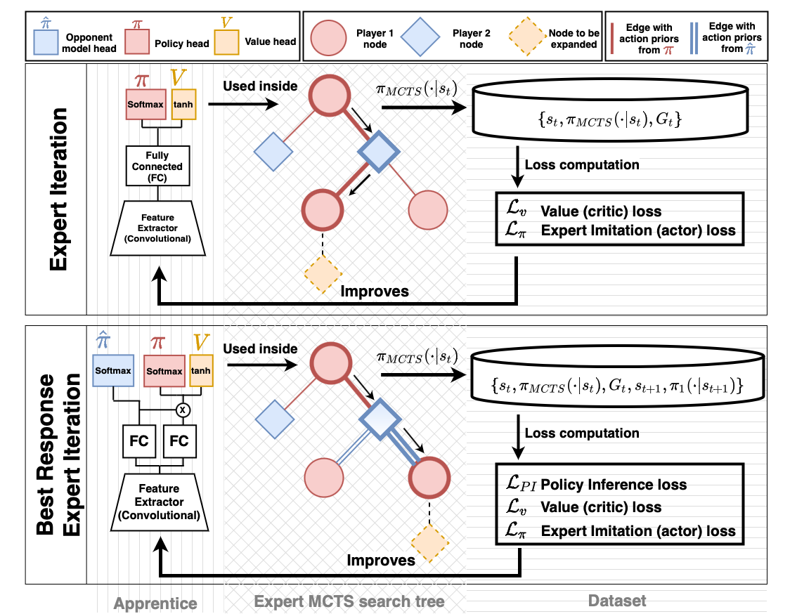
Figure 1: Illustration of ExIt (top half) and BRExIt (bottom half) for a 2-player game. BRExIt bases the decision on how to compute edge priors based on whose turn a node corresponds to. For opponent nodes, during training, these action priors can come from the true opponent’s policy or from the apprentice’s opponent model heads ${\color[rgb]{0,0,1}\hat{\pi}}$. BRExIt adds an opponent modelling loss by also gathering the states observed by the opponent $s_{t+1}$ and either the output of their policy $\pi_{1}(\cdot|s_{t+1})$, or a corresponding one-hot encoded action.

We present Best Response Expert Iteration (BRExIt), an extension on ExIt that uses opponent modelling for two purposes. First, to enhance the apprentice’s architecture with opponent modelling heads, acting as feature shaping mechanisms – see Subsection 4.1. Second, to allow the MCTS expert to approximate a best response against a set of opponents: $\pi_{MCTS}\in BR(\bm{\pi_{-i}})$ – see Subsection 4.3. We visually compare BRExIt and ExIt in Figure 1.

4.1 Learning opponent models in sequential games

Previous approaches to learn opponent models used observed actions as learning targets, coming from a game theoretical tradition where individual actions can be observed but not the policy that generated them Brown (1951). However, the centralized population-based training schemes which motivate our research already require access during training to all policies in the environment, both for the training agent and the opponents’ policies. We further exploit this assumption by separately testing two options for the learning targets in the policy inference loss from Equation 2: the one-hot encoded observed opponent actions, or the full distributions over actions computed by the opponents during play.

Prior work has typically focused on fully observable simultaneous games, where a shared environment state is used by all agents to compute an action at every timestep. Thus, if agent $i$ wanted to learn models of its opponents’ policies, storing (a) each of $i$’s observed shared states and (b) opponent actions, was sufficient to learn opponent models. We extend this to sequential games, where agents take turns acting based on individual states, in the following way. BRExIt augments the dataset collected by ExIt, specified in Equation 6, by adding (1) the state which each opponent agent $j\neq i$ observed and (2) either only the observed opponent actions or the full ground truth action distributions given by the opponent policies in their corresponding turn. The data collection process for sequential environments is described in Algorithm 1. Formally, for the BRExIt agent acting at timestep $t$ and its $n_{o}$ opponents acting at timesteps $t+1$ to $t+n_{o}$, BRExIt adds to its dataset either the observed action of every agent $j$, or their policy $\pi_{j}$ evaluated at the state of their turn.

$$\{s_{t},\pi_{MCTS}(\cdot|s_{t}),\{s_{t+j},\pi_{j}(\cdot|s_{t+j})\}^{n_{o}}_{j=1},G^{i}_{t}\}$$ (7)

4.2 Apprentice Representation

BRExIt’s three headed apprentice architecture extends ExIt’s actor-critic representation with opponent models as per DPIQN’s design Hernandez-Leal et al. (2019), depicted on the bottom left of Figure 1 for a single opponent. This architecture reuses parameters from the OM as a feature shaping mechanism for both the actor and the critic. It takes as input an environment state $s_{t}\in\mathcal{S}$ for a timestep $t$, which can correspond to the observed state of any agent. It features 3 outputs: (1) the apprentice’s actor policy $\pi_{\bm{\theta}}(s_{t})$ (2) the state-value critic $V^{\pi_{\bm{\theta}},\bm{\hat{\pi}_{\Psi}}}_{\bm{\phi}}(s_{t})$ (3) the opponent models $\hat{\pi}^{\bm{\psi}_{j}}(s_{t})\in\bm{\hat{\pi}^{\Psi}}$, where $\bm{\Psi}$ contains the parameters for all opponent models and $\psi_{j}\subset\bm{\Psi}$ the parameters for opponent model head $j$.

On certain sequential games the distribution of states encountered by each agent might differ, and so the actor-critic head and each of the OM heads could each be trained on different state distributions. In practice this means that the output of one of these heads might only be usable if the input state $s_{t}$ for a timestep $t$ comes from the distribution it was trained on; however, the OM can in any case help via feature shaping. This does not apply to simultaneous games where all agents observe the same state.

4.3 Opponent modelling inside MCTS

BRExIt follows Equation 8 to compute the action priors $P(s,a)$ from Equation 4 for a node with player index $j$, notably using opponent models in nodes within the search tree that correspond to opponents’ turns. This process is exemplified in the lower middle half of Figure 1. Such opponent models can be either the ground truth opponent policies (the real opponent policies $\bm{\pi_{-i}}$) by exploiting centralized training scheme assumptions, or otherwise the apprentice’s learnt opponent models $\bm{\hat{\pi}^{\psi}}$. This is a key difference from ExIt, which always uses the apprentice’s $\pi_{\bm{\theta}}$ to compute $P(s,a)$.

$$P(s,a)=\begin{cases*}\pi_{\bm{\theta_{\phantom{j}}}}(a|s)&$j$ == BRExIt player index\\ \pi^{j}_{-i}(a|s)&For ground truth models\\ \hat{\pi}^{\bm{\psi_{j}}}(a|s)&For learnt opponent models\end{cases*}$$ (8)

By using either the ground truth or learnt opponent models, we initially bias the search towards a best response against the actual policies in the environment. However, note that initial $P(s,a)$ values will be overridden by the aggregated simulation returns $Q(s,a)$, as with infinite compute MCTS converges to best response against a perfectly rational player, whose actions may deviate from the underlying opponent’s policy. Thus, BRExIt’s search maintains the asymptotic behaviour of MCTS while simultaneously priming the construction of the tree towards areas which are likely to be explored by the policies in the environment.

In contrast to BRExIt, ExIt biases its expert search towards a best response against the apprentice’s own policy, by using the apprentice $\pi_{\bm{\theta}}$ to compute $P(s,a)$ at every node in the tree. MCTS here assumes that all agents follow the same policy as the apprentice, whereas in reality agents might follow any arbitrary policy. Not trying to exploit the opponents it is trained against, ExIt generates more conservative searches. Recent studies show that this conservativeness can be detrimental in terms of finding diverse sets of policies throughout training for population-based training schemes Balduzzi et al. (2019); Liu et al. (2021). Instead, they advocate for a more direct computation of best responses against known opponents as a means to discover a wider area of the policy space. This allows the higher level training scheme to better decide on which opponents to use as targets to guide future exploration. We argue that BRExIt has this property built-in, by actively biasing its search towards a best response against ground truth opponent policies. Future work could investigate this claim.

We could have designed BRExIt to be even more exploitative towards opponent models, by masking actions sampled from these models as part of the environment dynamics. While this would yield actions very specifically targeted to respond to the modelled policies, it makes such best reponses very brittle, and can be problematic especially for imperfect OMs. In contrast, we propose using opponent models as priors in BRExIt, such that planning can still improve upon the opponent policies; this results in more robust learning targets.

Algorithms 1, 2 and 3 depict BRExIt’s data collection, model update logic and overarching training loop respectively for a sequential environment. Coloured lines represent our contributions w.r.t ExIt.

Input: $(\text{apprentice }\pi_{\bm{\theta}},{\color[rgb]{1,.5,0}\text{opp. models }\hat{\bm{\pi}}^{\bm{\psi}}_{-i}},\text{critic }V_{\bm{\phi}})$

Input: Opponent policies: $\bm{\pi_{-i}}$

Input: Environment: $E=(\mathcal{P},\rho_{0})$

1 Initialize dataset: $D=[\ ]$;

2 Initialize time $t\leftarrow 0$;

3 Sample initial state $s_{0}\sim\rho_{0}$;

4 while $s_{t}$ is not $terminal$ do

5       Search: $a_{t},tree=MCTS(s_{t},\pi_{\bm{\theta}},{\color[rgb]{1,.5,0}\bm{\pi_{-i}}},V_{\bm{\psi}})$;

6       Act in the game $s_{t+1},r_{t}\sim\mathcal{P}(s_{t},a_{t})$;

7       Get from $tree$: $\pi_{MCTS}(s_{t},a)=\frac{N_{root}(s_{t},a)}{\sum_{a^{\prime}}N_{root}(s_{t},a^{\prime})}$;

8       for $j=1,\ldots,|\bm{\pi_{-i}|}$ do

9             Sample opp. action: $a_{t+j}\sim\bm{\pi_{-i}}^{j}(s_{t+j})$;

10             Act in the game $s_{t+j},\_\sim\mathcal{P}(s_{t+j},a_{t+j})$

11       end for

12      $D\cup\{s_{t},\pi_{mcts}(s_{t}),$ $\{s_{t+j},\bm{\pi_{-i}}^{j}(s_{t+j})\}^{|\bm{\pi_{o}}|}_{j=1}$$,r_{i}\}$;

13       $t\leftarrow t+|\bm{\pi_{-i}}|$;

14      

15 end while

16return $D$;

Algorithm 1 BRExIt data collection

Input: Three head network: $NN=(\pi_{\bm{\theta}},{\color[rgb]{1,.5,0}\hat{\bm{\pi}}^{\bm{\psi}}_{-i}},V_{\bm{\phi}})$

Input: Dataset: $D$

1 for $t=0,1,2,\dots$ do

2      

3      Sample $n$ datapoints from $D$:

4       $(s_{t},r_{t},\pi_{MCTS}(s_{t},\cdot),r_{i},\linebreak{\color[rgb]{1,.5,0}\{s_{t+j},\bm{\pi_{-i}}^{j}(\cdot|s_{t+1})\}^{|\hat{\bm{\pi}}^{\bm{\psi}}_{-i}|}_{j=1}})_{1,\ldots,n}$;

5      

6      MSE value loss: $\mathcal{L}_{v}=(v-V_{\bm{\phi}}(s_{t}))^{2}$ ;

7      

8      CE policy loss $\mathcal{L}_{\pi}=\pi_{MCTS}(s_{t})\log{(\pi_{\bm{\theta}}(s_{t}))}$;

9      

10      CE policy inference loss: $\mathcal{L}_{PI}=\frac{1}{|\bm{\pi}_{-i}|}\sum^{|\bm{\pi_{-i}}|}_{j=1}\pi^{j}_{-i}(s_{t+j})\log{(\hat{\pi}^{\bm{\psi_{j}}}_{-i}(s_{t+j}))}$;

11      

12      Policy inference weight: $\lambda=\frac{1}{\sqrt{\mathcal{L}_{PI}}}$;

13      

14      Weighted final loss $\mathcal{L}_{total}={\color[rgb]{1,.5,0}\lambda}(\mathcal{L}_{v}+\mathcal{L}_{\pi})+{\color[rgb]{1,.5,0}\mathcal{L}_{PI}}$;

15      

16      Backpropagate $\nabla\mathcal{L}_{total}$ through $\bm{\theta},{\color[rgb]{1,.5,0}\bm{\psi}},\bm{\phi}$ ;

17      

18 end for

19

Algorithm 2 BRExIt model update

Input: Three head network: $NN=(\pi_{\bm{\theta}},{\color[rgb]{1,.5,0}\hat{\bm{\pi}}^{\bm{\psi}}_{-i}},V_{\bm{\phi}})$

Input: Opponent policies: $\bm{\pi}_{-i}$

1

2for $training\ iteration=0,1,2,\dots$ do

3       Algo. 1: $D=DatasetCollection(NN,{\color[rgb]{1,.5,0}\bm{\pi}_{-i}})$;

4       Algo. 2: $NN=UpdateApprentice(NN,D)$;

5      

6 end for

return NN

Algorithm 3 BRExIt training loop

5 Experiments & Discussion

We are trying to answer the following two questions: Primarily, is BRExIt more performant than ExIt at distilling a competitive policy against fixed opponents into its apprentice? Secondarily, are full distribution targets for learning opponent models preferable over one-hot action encodings?

The environment: We conducted our experiments in the fully observable, sequential two-player game of Connect4, which is computational amenable and possesses a high degree of skill transitivity Czarnecki et al. (2020). We decided on using a single environment in order to obtain statistically significant results through a larger number of runs over granular algorithmic ablations. We acknowledge the limitations of using a single test domain.

Test opponents: We generated two test agents $\pi_{weak},\pi_{strong}$ by freezing copies of a PPO Schulman et al. (2017) agent trained under $\delta=0$-Uniform self-play Hernandez et al. (2019) after 200k and 600k episodes. Motivated by population-based training schemes, we also used an additional opponent policy $\pi_{mixed}$, which randomly selects one of the test agents every episode.

Trained agents: We independently trained 7 types of agents for 48 wall-clock hours each, performing an additive construction from ExIt to BRExIt. ExIt is the original algorithm, ExIt-OMFS denotes ExIt using OMs only for feature shaping. BRExIt-OMS additionally uses learnt OMs during search and BRExIt uses the ground truth OMs during search. For the agents using OMs, we trained both a version using full action distributions as action targets and another with one-hot encoded action targets. Each algorithm was independently trained 10 times against the 3 test opponents, yielding a total of 280 training runs. Following statistical practices Agarwal et al. (2021) we use Inter Quartile Metrics (IQM) for all results, discarding the worst and best performing 25% runs to obtain performance metrics less susceptible to outliers.

5.1 On BRExIt’s performance vs. ExIt

To answer our first question, Figure 2 shows the evolution of the winrate of each of the ablation’s apprentice policies throughout training. A datapoint was computed every policy update (i.e every 800 episodes) by evaluating the winrate of the apprentice policy against the opponent over 100 episodes. (Note that the difference in number of episodes between all

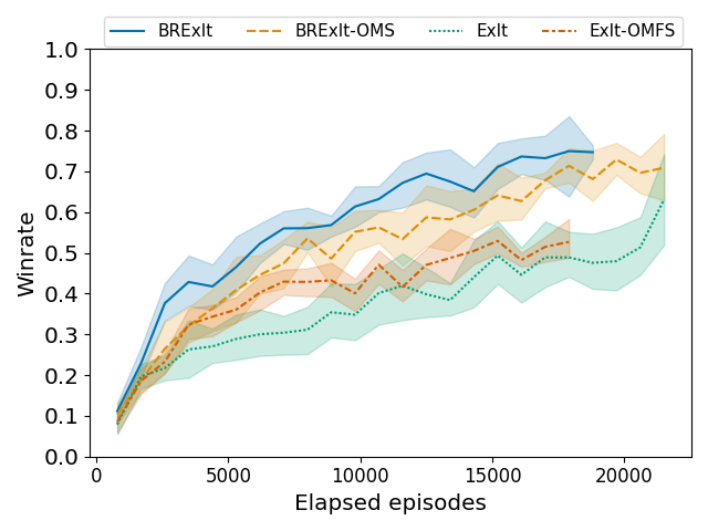
(a) VS Weak agent

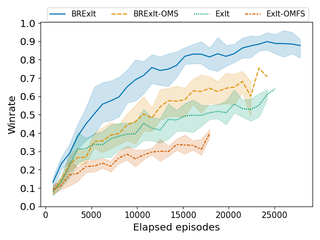
(b) VS Strong

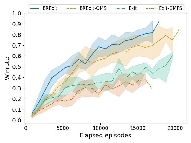
(c) VS Mixed

Figure 2: The evolution of winrates for each ablation during training vs fixed opponents for 48h wall-clock time. Lines represent the mean value the of final apprentice’s winrate over all runs. Higher is better; shaded areas show 95% bootstrap confidence intervals.

ablations depends on the average episode length over the 48h of training time, which can vary as a function of both players involved.) Figure 3 analyzes these results and shows the probability of improvement (PoI) that one ablation has over another, defined as the probability that algorithm $X$ would yield an apprentice policy which has a higher winrate against its training opponent that algorithm $Y$ Agarwal et al. (2021). All agents are using full distribution OM targets here.

Figure 2 shows that BRExIt style agents consistently achieve a higher winrate than ExIt agents. BRExIt regularly outperforms BRExIt-OMS (77% PoI), successfully exploiting the centralized assumption of having opponent policies available during search for extra performance. If opponent policies can only be sampled for training games but not during search, using learnt OMs during search is still beneficial, as we see that BRExIt-OMS consistently outperforms ExIt (90 % PoI). Surprisingly, ExIt-OMFS performs worse than ExIt by a significant margin (the latter has a 80% PoI against the former), providing empirical evidence that OMs with static opponents can be detrimental for ExIt if OMs are not exploited within MCTS. This goes against previous results Wu (2019), which explored OMs within ExIt merely as a feature shaping mechanism and claimed modest improvements when predicting the opponent’s follow-up move. Differences may be attributed to the fact that we model the opponent policy on the current state, instead of the next state.

In summary, with BRExIt (using ground truth OMs) and BRExIt-OMS (using learnt OMs) featuring a $>97\%$ and $>91\%$ PoI respectively against vanilla ExIt, our empirical results warrant the use of our novel algorithmic variants instead of ExIt whenever opponent policies are available for training.

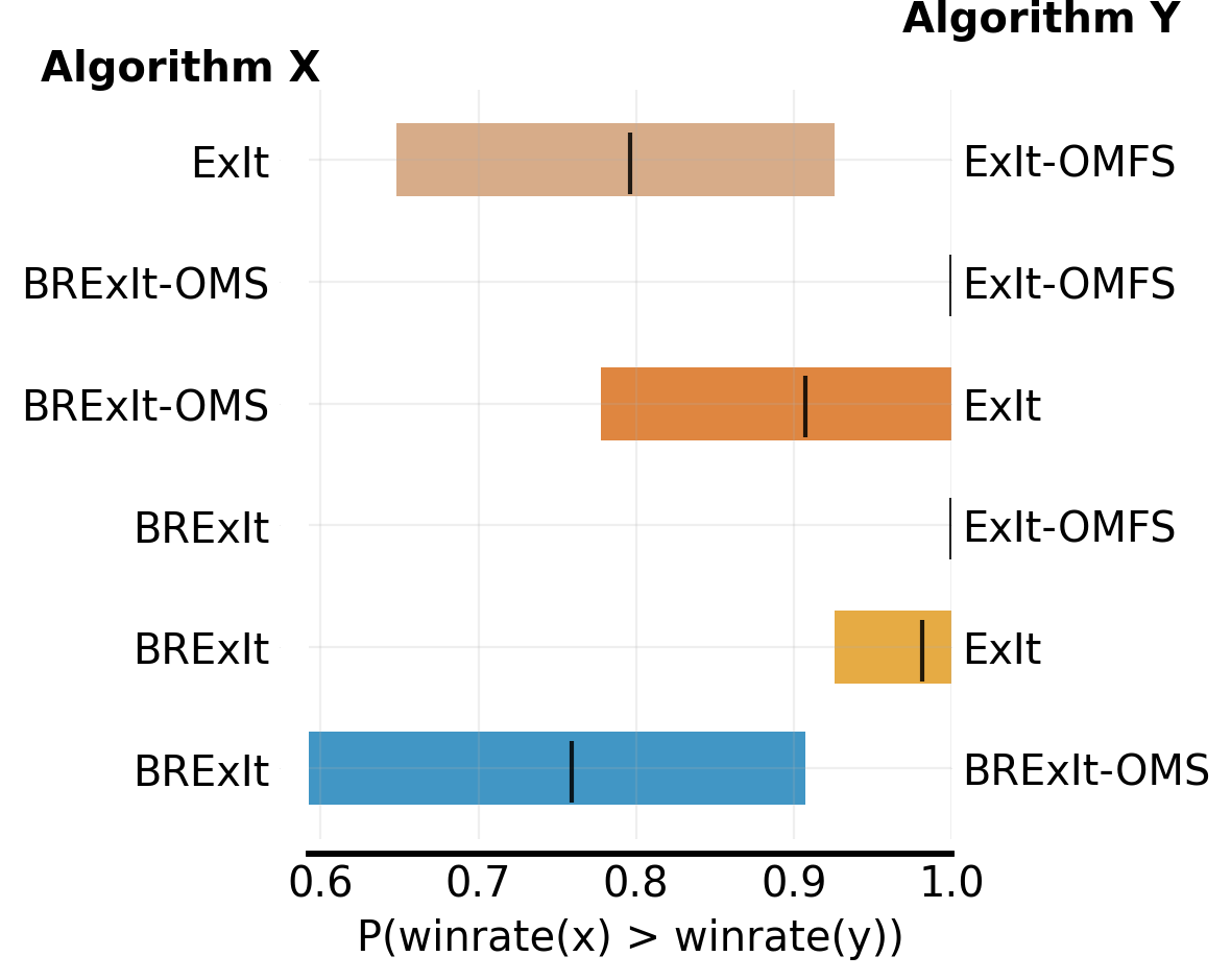
Figure 3: Each row shows the probability (vertical marker) that the algorithm $X$ (left) trains its apprentice’s policy to reach a higher winrate than algorithm $Y$ (right) after the allotted 48h. Colored bars indicate 95% bootstrap confidence intervals. Note that every training run for both BRExIt and BRExIt-OMS yielded higher performing policies than any run from ExIt-OMFS, and thus their comparisons have a 100% probability of improvement over ExIt-OMFS.

5.2 On full distribution VS one-hot targets

To answer our second question, we conducted Kolmogorov-Smirnov tests comparing full action distribution targets to one-hot encoded action targets for OMs. The samples we compared were the sets of winrates at the end of training, one datapoint per training run. Table 1 shows the results: There is no statistical difference between agents trained with algorithms using one-hot encoded OM targets when compared to using full action distributions. We obtain $p\gg 0.05$ for each algorithmic combination, so we cannot reject the null hypotheses that both data samples come from the same distribution; the only exception being ExIt-OMFS, which shows a statistically significant decrease in performance when using one-hot encoded targets.

These results run contrary to the intuition that richer targets for opponent models will in turn improve the quality of the apprentice’s policy. However, we observed that full distributional targets do yield OMs with better prediction capabilities, as indicated by lower loss of the OM during training. This hints at the possibility that OM’s usefulness increases only up to a certain degree of accuracy, echoing recent findings Goodman and Lucas (2020). Hence, while BRExIt does require access to ground truth policies during search, search in BRExIt-OMS achieves similar performance with opponent models trained on action observations, which is promising for transferring BRExIt-OMS into practical applications.

Table 1: Testing potential improvements of full distribution targets to one-hot encoded action targets. $p$-values are from two-sample Kolmogorov-Smirnov tests.

Base Algorithm	Opponent	$p$-value	Distr. targets
			signif. better?
BRExIt	Weak	0.930	No
BRExIt-OMS	Weak	0.931	No
ExIt-OMFS	Weak	0.930	No
BRExIt	Strong	0.930	No
BRExIt-OMS	Strong	0.999	No
ExIt-OMFS	Strong	0.930	No
BRExIt	Mixed	0.142	No
BRExIt-OMS	Mixed	0.930	No
ExIt-OMFS	Mixed	0.025	Yes

6 Conclusion

We investigated the use of opponent modelling within the ExIt framework, introducing the BRExIt algorithm. BRExIt augments ExIt by introducing opponent models both within the expert planning phase, biasing its search towards a best response against the opponent, and within the apprentice’s model, to use opponent modelling as an auxiliary task. In Connect4, we demonstrate BRExIt’s improved performance compared to ExIt when training policies against fixed agents.

There are multiple avenues for future work. At the level of population based training schemes (such as self-play), future work can focus on measuring whether the quality of populations generated by different training schemes using BRExIt surpasses that of populations where ExIt is used as a policy improvement operator. In addition, search methods can struggle with complex games due to their high branching factor – simultaneous move games for example have combinatorial action spaces – which could be alleviated by using BRExIt’s opponent models to narrow down the search space.

Appendix A Appendix

A.1 Training & benchmarking opponents

We used $\delta=0$-Uniform self-play Hernandez et al. [2019], both for training our agents with BRExIt and its various ablations, and for training our test opponents with PPO. This self-play scheme makes a copy of the learning agent at the end of each episode, and adds it to its population – the set of available policies to be used as training opponents. At the beginning of each training episode, a policy is randomly sampled from the population as opponent for the learning agent. This self-play scheme is effective for relatively simple games like Connect4, because it ensures that the learning agent continues to face all policies discovered during training, preventing catastrophic forgetting and cyclic policy evolution, which leads to transitively better strategies.

Initially, we generated three internally monotonically stronger test opponents $\bm{\pi^{test}}=[\pi_{0},\pi_{1},\pi_{2}]$, by freezing a copy of a PPO Schulman et al. [2017] agent trained under $\delta=0$-Uniform self-play after 200k, 400k, and 600k episodes respectively. Table 2 shows the hyperparameters used to train these agents. No formal hyperparameter sweep was conducted, and the final values were chosen after a few manual trials. We experimented with frame stacking to add a temporal dimension to the state space, but it was ultimately discarded as it lead to weaker agents for our compute budget.

Table 2: PPO hyperparameters used to generate test opponents. Empty entries in rightmost column indicate that a single value was used.

Hyperparameter name	Value	Values explored
Horizon (T)	$2048$	512, 1024, 2048
Adam stepsize	$10^{-5}$	-
Num. epochs	$10$	5, 10
Minibatch size	$256$	128, 256, 512
Discount ($\gamma$)	$0.99$	-
GAE parameter ($\lambda$)	$0.95$	-
Entropy coefficient	$0.01$	-
Clipping parameter ($\epsilon$)	$0.2$	-
Gradient norm clipping	$1$	1, 5
Channels	[3, 10, 20, 20, 20, 1]	-
Kernel sizes	[3, 3, 3, 3, 3]	-
Paddings	[1, 1, 1, 1, 1]	-
Strides	[1, 1, 1, 1, 1]	-
Residual connections	[0,1], [1,2], [2,3], [3,4]	-

To evaluate the relative strength of the test opponents, we computed their corresponding winrate evaluation matrix to study pair-wise agent performances, as shown in Figure 4. We see that later agents can consistently beat earlier versions. This shows a transitive improvement within the population of agents that emerges from our single training run. However, the nature of PPO agents is reactive, as there is no planning involved during their training. This means that agents can be internally better because they learn how to exploit specific weaknesses of previous agents, which might not be present in unrelated agents, for example agents generated via planning based methods such as BRExIt. Because BRExIt uses planning to choose its actions during training, we ultimately want to give a ranking to our test agents against MCTS based methods. In order to label our test agents with the labels of weak and strong used in the main text, we use MCTS equivalent strength, which we define as the computational budget (number of MCTS iterations) required for an MCTS agent using random rollouts to reach a given winrate against a given agent policy $\pi$.

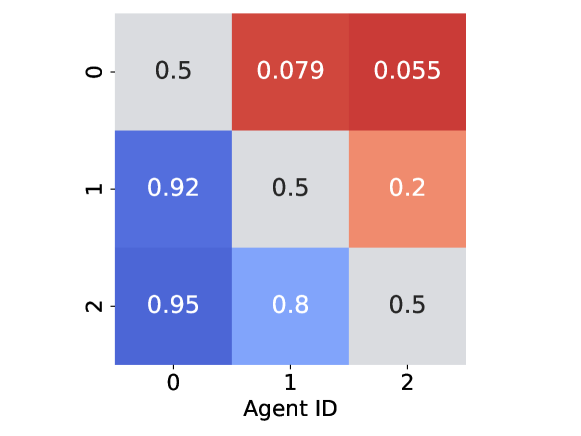
Figure 4: Winrates of $\pi_{\text{row}}$ against $\pi_{\text{column}}$, where each entry was computed by playing $1000$ head-to-head matches in the game of Connect4. The color of each agent (first player or second player) was chosen randomly at the beginning of each match to enforce symmetry. The agent IDs 0, 1 and 2 correspond to the 200K, 400K and 600K agents respectively.

Figure 5 shows a sweep of MCTS equivalent strength up to $80\%$ winrate. Surprisingly, we see that the test agent with only 200K training episodes, even though it is the weakest when matched directly against other agents from the test population as seen in Figure 4, is the strongest against MCTS with an MCTS equivalent strength of 95. We hypothesize that in the relatively low computational budgets that we have used for the agents trained in Section 5 of the main text, the heavily stochastic behaviour of the 200K agent can thwart shallow plans made by low budget MCTS agents. The MCTS equivalent strength for both other agents is 79. Given the superiority of the agent trained for 600K episodes in Figure 4 when compared to the agent trained for 400K, and their equivalent strengths against MCTS, we ultimately decided to discard the 400K agent as a test opponents for our main experiments. It is from this strength analysis against MCTS that we label the 600K and 200K agents as weak and strong respectively in the main paper.

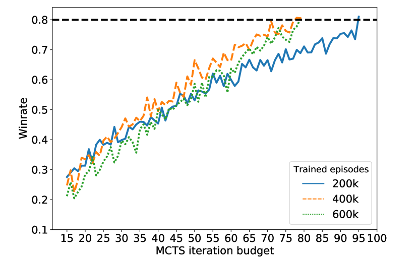
Figure 5: Evolution of winrate by MCTS against all candidate test agents (excluding $\pi_{mixed}$). As the MCTS computational budget increases on the horizontal axis, so does its playing strength. The black horizontal dashed line at the $80\%$ winrate mark is shown to compare the required budget to reach such winrate against all test opponents.

A.2 Neural network architectures

In order to level the playing field for all algorithms, we adjusted the actor-critic architecture, used by ExIt, and the opponent modelling enhanced actor-critic architecture, used by BRExIt and its ablations, to feature a similar number of parameters (approximately 27,000 trainable parameters).

The game of Connect4 is played on a $6\times 7$ grid, and each grid position can either be empty, occupied by one of player 1’s chips, or by one of player 2’s chips. The input to PPO’s and BRExIt’s neural network models was a $3\times 6\times 7$ tensor (a 3 channeled $6\times 7$ grid): The first channel features $0$s on all non-empty positions and $1$s on empty positions; the second channel features $1$s on positions taken by the current player and $0$s everywhere else; the third channel features $1$s on positions taken by the opponent and $0$s everywhere else.

We used a similar network architecture to Hernandez et al. [2019]. The input tensor was put through 5 convolutional layers, with residual connections skipping every other layer. Extra details are shown in Table 2. The output embedding found at the end of the last convolutional layer was fed into two parallel layers. One was a fully connected layer with a softmax activation function which represented the agent’s policy (the actor). The other was a single neuron and no activation function representing a state-value function (the critic).

Table 3: BRExIt, BRExIt-OMS, ExIt and ExIt-OMFS hyperparameters. Hyperparameter tuning was done manually and in a limited way due to limited computational resources. Empty entries in the rightmost column indicate that a single value was used. The neural network architecture shared across all agents was adapted from the original DPIQN Hong et al. [2018].

Hyperparameter name	Value	Values explored
MCTS budget	50	30, 50, 80
MCTS rollout budget	0	$\infty$, 0
MCTS exploration factor	2.	$1,2,5$
Dirichlet noise	False	True, False
Batch size	512	128, 256, 512
Espisodes per generation (train every $n$ episodes)	800	300, 500, 800, 1000
Epochs per iteration	5	1, 3, 5, 10
Reduce temperature after $n$ moves	10	$\infty$, 10
Channels	[12, 15, 20, 20, 20, 1]	-
Kernel sizes	[3, 3, 3, 3, 3]	-
Paddings	[1, 1, 1, 1, 1]	-
Strides	[1, 1, 1, 1, 1]	-
Residual connections	[[0,1], [1,2], [2,3], [3,4]]	-
Learning rate	1.5e-3	1e-3, 1.5e-3
Post feature extractor hidden units	[128, 128, 128]	-
Post feature extractor policy inference hidden units	[128, 64]	-
Post feature extractor actor critic hidden units	[128, 64]	-
Activation function	ReLu	-
Critic activation function	tanh	-
Gradient norm clipping	1	None, 1, 5

A.3 Kolmogorov-Smirnov test

Table 1 in Section 5 shows the $p$-values corresponding to the different two-sided Kolmogorov-Smirnov tests. This test measures if there is a significant statistical difference between 2 distributions $f(x)$ and $g(x)$. In our case, $f,g$ correspond to an algorithmic ablation (i.e BRExIt, BRExIt-OMS and ExIt-OMFS), with $g$ representing the same ablation as $f$ but using one hot action encodings for OM targets instead of full action distributions. $x$ denotes a test agent policy ($\pi_{weak},\pi_{strong}$ or $\pi_{mixed}$). Hence, $f(x),g(x)$ denote the stochastic functions that determine the final winrate obtained by $f$ or $g$ respectively at the end of a training run against policy $x$. Each of the 6 training runs used for each algorithmc ablation (originally 10, but we discard the top and bottom 2 performing runs as per Agarwal et al. [2021]) gives us one data point. Thus, our comparisons are between sets of 6 datapoints $f(x)=[f_{1}(x),f_{2}(x),f_{3}(x),f_{4}(x),f_{5}(x),f_{6}(x)]$ and similarly $g(x)=[g_{1}(x),g_{2}(x),g_{3}(x),g_{4}(x),g_{5}(x),g_{6}(x)]$.

A.4 Hyperparameters and general performance improvements

Deep reinforcement learning algorithms require a large amount of simulated experiences to train policies, and more so for deep multi-agent reinforcement learning. This is further exacerbated when planning based algorithms are used as part of RL algorithms, as is the case with MCTS within BRExIt. A single step in the main game requires many simulated games inside of MCTS. On top of this, RL methods do not tend to be robust to hyperparameters, requiring a lot of manual tuning and stabilizing implementation details. Because of this, it is common place to add ad-hoc or environment specific methods to reduce the amount of compute required to train policies and to increase their robustness. Here we present some performance improvements shared across all algorithmic ablations, which are orthogonal to the novel contributions presented in this paper but were nonetheless required to train our agents within our computational budget. We argue that these improvement methods benefit all ablations equally, and thus do not affect our comparisons. We present them here for completeness and to aid reimplementations efforts. The set of hyperparameters used for all algorithmic ablations during the final training run is present in Table 3.

A.4.1 Reducing exploration: removing Dirichlet noise on MCTS root priors

The algorithm AlphaGo Silver et al. [2018] introduced the notion of adding noise to the prior probabilities in the root node. By adding noise, we modify the priors over actions used in the selection phase, given by the apprentice’s state-value function. This is used as an exploration mechanism, by redistributing some probability weight given by the priors over all valid actions. The Dirichlet distribution is used to sample that noise: $P(s,a)=0.25*Dirichlet(\alpha)+0.75*P(s,a)$, where $\alpha=\sqrt{2}$. During an MCTS search with many hundreds of iterations (as was the case with AlphaZero), the explorative effects of this Dirichlet noise on the root node’s priors would eventually be washed out by state evaluations propagated upwards from further down the tree. In our case however, due to our relatively low MCTS budget of 50, we cannot afford to use Dirichlet noise, as this exploratory noise would randomize the output policy of the search $\pi_{MCTS}$ too much.

A.4.2 Sample efficiency: Data augmentation via exploiting state space symmetries

The board of Connect4, a $6\times 7$ matrix, is symmetrical over the vertical axis. We can exploit this to reduce the complexity of the environment. Let’s define a function over states $\sigma(\mathcal{S})\rightarrow\mathcal{S}$ which swaps columns with indexes $[1,2,3]$ with those with index $[7,6,5]$; and also over policies $\sigma(\Pi)\rightarrow\Pi$ by also swapping the probability weight over those column indices. Strategically speaking, the swapped situations are identical. AlphaZero was shown to be able to naturally learn this symmetry over enough training episodes Silver et al. [2018]. We add this symmetry a priori into our algorithm to reduce computational costs. This is done by augmenting every data point at the time it is appended to the replay buffer by also adding a copy with the corresponding symmetric transformation, on both the state and the policy target (and the opponent policy target in case of BRExIt). The value target remains the same. Formally, for every data point we obtain a tuple:

$$\{s_{t},\pi_{MCTS}(\cdot|s_{t}),G^{i}_{t}\}\rightarrow$$

$$(\{s_{t},\pi_{MCTS}(\cdot|s_{t}),G^{i}_{t}\},\{\sigma(s_{t}),\sigma(\pi)_{MCTS}(\cdot|s_{t}),G^{i}_{t}\})$$

A.4.3 Variance reduction on value targets: Averaging MCTS estimated returns with episodic returns

In the original ExIt specification, as described in Equation 6, at every timestep of each training episode, the following information is stored in a replay buffer: $\{s_{t},\pi_{MCTS}(\cdot|s_{t}),G^{i}_{t}\}$, where $G^{i}_{t}$ denotes player $i$’s total reward observed at the end of the episode. What this means for our state value function $V(s_{t})$ is that we are regressing all observed states in an episode $[s_{0},s_{1},\ldots]$ to the same value $G^{i}_{t}$. This target features a large variance, as we are mapping potentially dozens of states to the same target value. We can reduce the variance, with the downside of introducing some bias, by re-using state-dependent computation from each state-dependent MCTS call, meaning that we don’t use the same value target for each state anymore. For every data point we substitute $G^{i}_{t}$ by another variable $z^{i}_{t}$, for which we tried three different alternatives:

$$z^{i}_{t}=\frac{1}{2}*(\underbrace{\sum_{a\in\mathcal{A}}\pi_{MCTS}(a|s)*Q(s,a)}_{\textrm{Definition of $V^{\pi_{MCTS}}(s)$}}+G^{i}_{t})$$ (9)

First, we averaged the original target with the root node value of MCTS. This includes the value of sub-optimal actions that were sampled during exploration. This in turn induced pessimism in $V(s)$ estimations by our trained critics $V_{\bm{\phi}}(s)$, leading them to consistently estimate lower winrates than observed in practice.

$$z^{i}_{t}=\frac{1}{2}*(\underbrace{\text{max}_{a\in\mathcal{A}}*Q(s,a)}_{\textrm{Greedy w.r.t $Q(s,\cdot)$}}+G^{i}_{t})$$ (10)

Second, we tried using the value of the root node’s highest valued child node. This also introduced a bias, although this time in a positive direction, because the policy that will actually be followed corresponds to MCTS’s normalized child visitations (Equation 5) – which will put some probability weight on lower valued child nodes as well.

$$z^{i}_{t}=\frac{1}{2}*(\underbrace{Q(s,\operatorname*{arg\,max}_{a\in\mathcal{A}}N(s,a))}_{\textrm{MCTS action selection}}+G^{i}_{t})$$ (11)

Ultimately, we decided to average the episode returns with the $Q(s,a)$ value associated with the action actually selected and returned by MCTS. In our experiments, this was the most visited action at the root. Theoretically this still yields biased targets, as our actors $\pi_{\bm{\theta}}$ imitate an MCTS derived policy $\pi_{MCTS}$ while our critic $V_{\bm{\phi}}$ will regress against state-values that do not exactly match the actions taken by $\pi_{MCTS}$. However, not only did this seem to work well in practice, but we saw little to no bias in our critic’s estimations compared to the real episode returns using this bootstrapped estimate.

A.4.4 Extra exploitation: Temperature parameter

It is beneficial to have a high degree of exploration on the initial states of an environment, specially during early stages of training. The policy targets derived from normalized child visits at the root node $\pi_{MCTS}$ feature a high degree of exploration, especially with our low computational budget, as MCTS would discard low quality moves given larger computational budgets. This is convenient early during training for the aforementioned exploration on initial states, but can slow down the learning of exploitative policies against fixed agents. Thus, ideally we would like to focus initial moves on exploration, and switch to exploitation later into an episode.

We achieve this with temperature parameter $\tau$, which we use to exponentiate the visits to root node children before they are normalized:

$$\pi_{MCTS}(a|s)=\frac{N(s,a)^{1/\tau}}{\sum_{a^{\prime}}N(s,a^{\prime})^{1/\tau}}$$ (12)

We set $\tau=1$ for the first 10 moves, after which we reduce it to $\tau=0.01$, which effectively moves all probability weight to the most visited action. Therefore, the first 10 moves will feature increased exploration, and all other moves will focus on the most-visited action. We note that there exists research on this area, with a focus on removing exploration elements from MCTS policy targets with the hope of aiding interpretability Soemers et al. [2019].

A.4.5 Gradient norm clipping

Many RL algorithms which involve computing gradients with respect to a loss function suffer from high variance in the estimation of these gradients. If the parameters of a model are updated by applying gradients of a large magnitude, these might move the model’s parameters too far, even into poor performing sections of the parameter space. A proposed solution is to introduce gradient clipping Pascanu et al. [2013]. Its most naive implementation involves clipping the value of each individual gradient to a hyperparameter threshold $c$. A more nuanced alternative is gradient norm clipping. It involves concatenating all gradients of all parameters into a single vector $\bm{g}$. If the vector’s $n$th norm is greater than a threshold value $c$, then the vector is normalized according to:

$$\bm{g}=\begin{cases}\bm{g}\quad&\text{if}||\bm{g}||_{n}\leq c\\ c\frac{\bm{g}}{||\bm{g}||_{n}}&\text{otherwise}\\ \end{cases}$$ (13)

For all experiments we used the $L_{2}$ norm. We tried thresholds of $5$, $3$ and $1$. Even though we found that higher thresholds yielded a sharper increase in performance early on, a threshold of $c=1$ ended up achieving better stability and final performance than the other values.

A.4.6 Parallel data generation: Parallelized MCTS with centralized apprentice

We simulate multiple games of Connect4 in parallel, With every MCTS procedure running on an individual CPU core. A single process hosts the apprentice’s neural network, acting as a server, whose only function is to receive states from all MCTS processes. These are evaluated for (1) node priors $P(s,a)$ and (2) state evaluations $V(s)$. It busy polls all connections to MCTS processes for incoming states, batching all requests into a single neural network forward pass. This allows us to scale horizontally, theoretically linearly with the number of available CPUs. Because of the size of the network, Connect4’s small state size and the average batch size, we saw no performance improvement hosting the apprentice in CPU vs GPU. Surprisingly, our main bottleneck came from Python’s communication of PyTorch tensors among processes, stalling MCTS speed while requesting node evaluations $V(s)$ and node prior generations $P(s,a)$.

A.5 Description of computational infrastructure

The experiments presented in this publication were carried out in Snellius, the Dutch National supercomputer, a SLURM based computing cluster. Each of the 280 runs from Section 5 were individual SLURM jobs that run for 48h. They each had access to 1280GB of RAM and 64 CPUs with no GPUs.

References

- Agarwal et al. [2021] Rishabh Agarwal, Max Schwarzer, Pablo Samuel Castro, et al. Deep reinforcement learning at the edge of the statistical precipice. Advances in Neural Information Processing Systems, 34, 2021.
- Albrecht and Stone [2018] Stefano V Albrecht and Peter Stone. Autonomous agents modelling other agents: A comprehensive survey and open problems. Artificial Intelligence, 258:66–95, 2018.
- Anthony et al. [2017] Thomas Anthony, Zheng Tian, and David Barber. Thinking fast and slow with deep learning and tree search. In NIPS, 2017.
- Balduzzi et al. [2019] David Balduzzi, Marta Garnelo, Yoram Bachrach, et al. Open-ended learning in symmetric zero-sum games. In International Conference on Machine Learning, pages 434–443. PMLR, 2019.
- Berner et al. [2019] Christopher Berner, Greg Brockman, Brooke Chan, et al. Dota 2 with large scale deep reinforcement learning. arXiv preprint arXiv:1912.06680, 2019.
- Brown [1951] George W Brown. Iterative solution of games by fictitious play. Activity analysis of production and allocation, 13(1):374–376, 1951.
- Browne et al. [2012] Cameron B Browne, Edward Powley, Daniel Whitehouse, et al. A survey of Monte Carlo Tree Search methods. IEEE Transactions on Computational Intelligence and AI in Games, 4(1):1–43, 2012.
- Carroll et al. [2019] Micah Carroll, Rohin Shah, Mark K Ho, et al. On the utility of learning about humans for human-ai coordination. In Advances in Neural Information Processing Systems, pages 5175–5186, 2019.
- Czarnecki et al. [2020] Wojciech M Czarnecki, Gauthier Gidel, Brendan Tracey, et al. Real world games look like spinning tops. Advances in Neural Information Processing Systems, 33:17443–17454, 2020.
- Espeholt et al. [2018] Lasse Espeholt, Hubert Soyer, Remi Munos, et al. IMPALA: Scalable Distributed Deep-RL with Importance Weighted Actor-Learner Architectures. CoRR, abs/1802.01561, 2018.
- Goodman and Lucas [2020] James Goodman and Simon Lucas. Does it matter how well I know what you’re thinking? opponent modelling in an RTS game. In IEEE Congress on Evolutionary Computation, CEC 2020, pages 1–8. IEEE, 2020.
- He et al. [2016] He He, Jordan Boyd-Graber, Kevin Kwok, and Hal Daumé III. Opponent modeling in deep reinforcement learning. In International Conference on Machine Learning, pages 1804–1813, 2016.
- Hernandez et al. [2019] Daniel Hernandez, Kevin Denamganaï, Yuan Gao, et al. A generalized framework for self-play training. In 2019 IEEE Conference on Games (CoG), pages 1–8. IEEE, 2019.
- Hernandez-Leal et al. [2017] Pablo Hernandez-Leal, Michael Kaisers, Tim Baarslag, and Enrique Munoz de Cote. A survey of learning in multiagent environments: Dealing with non-stationarity. arxiv 2017. arXiv preprint arXiv:1707.09183, 2017.
- Hernandez-Leal et al. [2019] Pablo Hernandez-Leal, Bilal Kartal, and Matthew E. Taylor. Agent modeling as auxiliary task for deep reinforcement learning. In Gillian Smith and Levi Lelis, editors, Proceedings of the Fifteenth AAAI Conference on Artificial Intelligence and Interactive Digital Entertainment, AIIDE 2019, pages 31–37. AAAI Press, 2019.
- Hong et al. [2018] Zhang-Wei Hong, Shih-Yang Su, Tzu-Yun Shann, et al. A deep policy inference q-network for multi-agent systems. In Proceedings of the 17th International Conference on Autonomous Agents and MultiAgent Systems, pages 1388–1396. International Foundation for Autonomous Agents and Multiagent Systems, 2018.
- Lanctot et al. [2017] Marc Lanctot, Vinicius Zambaldi, Audrunas Gruslys, et al. A unified game-theoretic approach to multiagent reinforcement learning. Advances in Neural Information Processing Systems, 30:4190–4203, 2017.
- Liu et al. [2021] Xiangyu Liu, Hangtian Jia, Ying Wen, et al. Towards unifying behavioral and response diversity for open-ended learning in zero-sum games. Advances in Neural Information Processing Systems, 34, 2021.
- Mnih et al. [2013] Volodymyr Mnih, Koray Kavukcuoglu, David Silver, et al. Playing Atari with Deep Reinforcement Learning. CoRR, abs/1312.5602, 2013.
- Nashed and Zilberstein [2022] Samer Nashed and Shlomo Zilberstein. A survey of opponent modeling in adversarial domains. Journal of Artificial Intelligence Research, 73:277–327, 2022.
- Oliehoek and Amato [2014] Frans A Oliehoek and Christopher Amato. Best response bayesian reinforcement learning for multiagent systems with state uncertainty. In Proceedings of the Ninth AAMAS Workshop on Multi-Agent Sequential Decision Making in Uncertain Domains (MSDM), 2014.
- Pascanu et al. [2013] Razvan Pascanu, Tomas Mikolov, and Yoshua Bengio. On the difficulty of training recurrent neural networks. In International conference on machine learning, pages 1310–1318. PMLR, 2013.
- Schaul et al. [2015] Tom Schaul, John Quan, Ioannis Antonoglou, and David Silver. Prioritized Experience Replay. CoRR, abs/1511.05952, 2015.
- Schulman et al. [2017] John Schulman, Filip Wolski, Prafulla Dhariwal, et al. Proximal policy optimization algorithms. CoRR, abs/1707.06347, 2017.
- Silver et al. [2016] David Silver, Aja Huang, Chris J Maddison, et al. Mastering the game of Go with deep neural networks and tree search. Nature, 529(7587):484–489, 2016.
- Silver et al. [2018] David Silver, Thomas Hubert, Julian Schrittwieser, et al. Mastering Chess and Shogi by Self-Play with a General Reinforcement Learning Algorithm. Science, 362:1140–1144, 2018.
- Soemers et al. [2019] Dennis JNJ Soemers, Eric Piette, Matthew Stephenson, and Cameron Browne. Learning policies from self-play with policy gradients and mcts value estimates. In 2019 IEEE Conference on Games (CoG), pages 1–8. IEEE, 2019.
- Soemers et al. [2020] Dennis JNJ Soemers, Éric Piette, Matthew Stephenson, and Cameron Browne. Manipulating the distributions of experience used for self-play learning in expert iteration. arXiv preprint arXiv:2006.00283, 2020.
- Timbers et al. [2022] Finbarr Timbers, Nolan Bard, Edward Lockhart, et al. Approximate exploitability: Learning a best response. In Proceedings of the International Joint Conference on Artificial Intelligence (IJCAI), pages 3487–3493, 2022.
- Vinyals et al. [2019] Oriol Vinyals, Igor Babuschkin, Wojciech M Czarnecki, et al. Grandmaster level in starcraft ii using multi-agent reinforcement learning. Nature, 575(7782):350–354, 2019.
- Willemsen et al. [2021] Daniel Willemsen, Hendrik Baier, and Michael Kaisers. Value targets in off-policy alphazero: a new greedy backup. Neural Computing and Applications, pages 1–14, 2021.
- Wu [2019] David J Wu. Accelerating self-play learning in go. arXiv preprint arXiv:1902.10565, 2019.