Relaxation of phonons in the Lieb-Liniger gas by dynamical refermionization

Abstract

Motivated by recent experiments, we investigate the Lieb-Liniger gas initially prepared in an out-of-equilibrium state that is Gaussian in terms of the phonons, namely whose density matrix is the exponential of an operator quadratic in terms of phonons creation and anihilation operators. Because the phonons are not exact eigenstates of the Hamiltonian, the gas relaxes to a stationary state at very long times whose phonon population is a priori different from the initial one. Thanks to integrability, that stationary state needs not be a thermal state. Using the Bethe Ansatz mapping between the exact eigenstates of the Lieb-Liniger Hamiltonian and those of a non-interacting Fermi gas and bosonization techniques we completely characterize the stationary state of the gas after relaxation and compute its phonon population distribution. We apply our results to the case where the initial state is an excited coherent state for a single phonon mode, and we compare them to exact results obtained in the hard-core limit.

Introduction.

Phonons are a central concept in the field of quantum gases. They are quantized sound waves, or collective phase-density excitations, that arise in low-energy and long wave-length description of quantum gases, e.g. in Bogoliubov theory of Bose-Einstein condensates in $D\geq 2$ spatial dimensions Pitaevskii and Stringari (2016), or, in 1D, in Bogoliubov theory for quasi-condensates Popov (1987); Mora and Castin (2003) and more generally in Luttinger liquid theory Haldane (1981); Cazalilla (2004); Cazalilla et al. (2011). Phonons are routinely used to analyze experiments with out-of-equilibrium quantum gases, such as the dynamics generated by a quench of the interaction strength in a 1D Bose gas Schemmer et al. (2018), or by its splitting into two parallel clouds Langen et al. (2013); Rauer et al. (2018), or by a quench of the external potential Cataldini et al. (2021). In general, the description in terms of phonons accounts remarkably well for the observed short time dynamics Rauer et al. (2018); Geiger et al. (2014). Crucially, the out-of-equilibrium states produced in these experimental setups are phononic Gaussian states with expectation values of phononic operators obeying Wick’s theorem. This is because they are obtained from a thermal equilibrium state, which is itself described by a Gaussian density matrix, by acting on it with linear or quadratic combinations of density and/or phase field.

However, although phonons are exact eigenstates of the effective low-energy Hamiltonian, they are only approximations of the true eigenstates of the microscopic Hamiltonian. Thus, phonons have finite lifetime Andreev (1980); Samokhin (1998); Ristivojevic and Matveev (2014, 2016); Micheli and Robertson (2022) and, at long times, the phonon distribution should evolve. In ergodic systems, this evolution would consist in the relaxation towards thermal equilibrium. But what if the microscopic system is integrable? In this paper, we investigate the integrable Lieb-Liniger model of 1D Bosons with contact repulsive interactions Lieb and Liniger (1963). We express the phonons in terms of the true, i.e. infinite-lifetime, quasi-particles of the Lieb-Liniger model. We can then characterize the final stationary state of the system after relaxation and we relate the phonon mode occupations to the ones in the initial state.

Sketch of the main result.

The Hamiltonian of the Lieb-Liniger model is

$$H=\int_{0}^{L}dx\leavevmode\nobreak\ \Psi^{\dagger}\left(-\frac{1}{2}\partial_{x}^{2}+\frac{c}{2}\Psi^{\dagger}\Psi\right)\Psi,$$ (1)

with second-quantized bosonic operators obeying commutation relations $[\Psi(x),\Psi^{\dagger}(y)]=\delta(x-y)$. Here $c>0$ is the repulsion strength, $L$ is the length of the system (we use periodic boundary conditions) and we use units such that $\hbar=m=1$. For $N$ atoms the average density is $\rho_{0}=N/L$. The density fluctuation and current operators are

$$\delta\rho(x) = \Psi^{\dagger}(x)\Psi(x)-\rho_{0},$$

$$J(x) = \frac{i}{2}\left[(\partial_{x}\Psi^{\dagger}(x))\Psi(x)-\Psi^{\dagger}(x)(\partial_{x}\Psi(x))\right].$$ (2)

At low temperature, it is customary to think of low-energy and long wavelength excitations above the ground state as quantized sound waves (phonons) that move to the right or to the left at the sound velocity $v$. The chiral combinations

$$J_{\rm R/L}(x)=\frac{1}{2}\left(v\leavevmode\nobreak\ \delta\rho(x)\pm J(x)\right)$$ (3)

are the currents carried by right-moving (R) or left-moving (L) quasi-particles, with Fourier modes

$$J_{\rm R}(x)=\frac{v\sqrt{K}}{L}\sum_{n>0}\sqrt{n}\left(e^{i\frac{2\pi nx}{L}}A_{{\rm R},n}+e^{-i\frac{2\pi nx}{L}}A^{\dagger}_{{\rm R},n}\right),$$ (4)

with $n>0$ (a similar definition holds for $A_{{\rm L},n}$). Here $K=\pi\rho_{0}/v$ is the Luttinger parameter. Acting with $A^{\dagger}_{\mathrm{R/L},n}$ on the ground state $\left|0\right>$, one generates R/L-phonons. We stress that the excited states generated this way are only approximations of the true eigenstates of the Lieb-Liniger Hamiltonian (1). The lifetime of phonons may be large, but it is not infinite, so the phonon population will evolve, until it ultimately reaches a stationary value, governed by the true eigenstates of the Lieb-Liniger model.

Our main result is a general formula that relates the phonon population at infinite time to the one in the initial state. The latter is assumed to be Gaussian in terms of phonons, such that correlation functions of products of operators $J_{\rm R/L}(x)$ reduces to sums of products of one- and two-point correlation functions by Wick’s theorem. In the special case of a translation-invariant initial state $\left<.\right>_{0}$, populated by R-phonons, parametrized by a single function $g(x)$ via  

$$\left<J_{\rm R}(x)J_{\rm R}(y)\right>_{0}\,=\,-\frac{\rho_{0}v}{4\pi}\partial_{x}^{2}g(x-y),$$ (5)

and $\expectationvalue{J_{R}(x)}_{0}=0$, our result is that the two-point function ultimately relaxes to

$$\left<J_{\rm R}(x)J_{\rm R}(y)\right>_{\infty}\,=\,\frac{\pi\rho_{0}v}{L^{2}}\exp\left(2g(x-y)\right).$$ (6)

Thus, the phonon population evolves, unless the function $g(x)$ satisfies $\partial_{x}^{2}g=-(4\pi^{2}/L^{2})e^{2g}$. One solution to this equation is the thermal distribution at inverse temperature $\beta\ll L/v$, for which $g(x-y)=-\log\left(\frac{2\beta v}{iL}\sinh\left(\frac{\pi(x-y)}{\beta v}\right)\right)$ Giamarchi (2003). So the thermally occupied phonon modes will not evolve, but more general initial states will show a relaxation phenomenon.

In the rest of this Letter we derive Eq. (6) and its generalisation to initial Gaussian phononic states not necessarly translationally invariant. We compare our predictions to exact numerical results obtained in the hard-core (Tonks-Girardeau) limit for an state with a single phononic mode initially displaced. We conclude by discussing perspectives for experimental observation of the evolution of phonon populations.

Eigenstates of the Lieb-Liniger model and Bethe fermions.

For even/odd $N$, an $N$-particle eigenstate of (1) is specified by an ordered set of half-integers/integers $I_{1}<I_{2}<\ldots<I_{N}$ which uniquely determines the set of $N$ rapidities $\lambda_{1}<\lambda_{2}<\ldots<\lambda_{N}$ via the Bethe equations Lieb and Liniger (1963); Gaudin (2014); Korepin et al. (1997)

$$\lambda_{a}+\frac{1}{L}\sum_{b=1}^{N}{\rm arctan}\left(\frac{\lambda_{a}-\lambda_{b}}{c}\right)\,=\,\frac{2\pi}{L}I_{a}\,.$$ (7)

The energy of that eigenstate is $E_{\{\lambda_{a}\}}=\sum_{a}\lambda_{a}^{2}/2$ and the corresponding wavefunction is $\left<{\rm vacuum}\right|\prod_{j=1}^{N}\Psi(x_{j})\left|\{\lambda_{a}\}\right>\,\propto\sum_{\sigma}\mathcal{A}_{\sigma}e^{i\sum_{a}\lambda_{\sigma(a)}x_{a}}$, where the sum is over all permutations $\sigma$ of $N$ elements and $\mathcal{A}_{\sigma}=\prod_{a>b}\left(1-ic\leavevmode\nobreak\ {\rm sgn}(x_{a}-x_{b})/(\lambda_{\sigma(a)}-\lambda_{\sigma(b)})\right)$. In the following we assume $N$ even. The ground state corresponds to densely packed Bethe half-integers $\{I^{(0)}_{a}\}\,=\,\left\{-\frac{N-1}{2},-\frac{N-1}{2}+1,\dots,\frac{N-1}{2}\right\}$.

Eq. (7) provides a one-to-one mapping between the eigenstates $\ket{\{I_{a}\}}$ of the Lieb-Liniger model and the eigenstates of $N$ non-interacting fermions with momenta $2\pi I_{a}/L$, $a=1,\ldots,N$. This mapping preserves the total momentum $P_{\{\lambda_{a}\}}=\sum_{a}\lambda_{a}=(2\pi/L)\sum_{a}I_{a}$. It is natural to introduce fermion operators $b_{J}$ that act on the normalized eigenstate $\ket{\{I_{a}\}}$ by removing a Bethe half-integer $J$ from the set $\{I_{a}\}$, if it is present, and by annihilating the state otherwise. Conversely, the operator $b^{\dagger}_{J}$ inserts $J$ in the set $\{I_{a}\}$ unless it is already present. The eigenstate corresponding to the modified state is then multiplied by $(-1)^{n_{I_{a}<J}}$, where $n_{I_{a}<J}$ is the number of elements of $\{I_{a}\}$ smaller than $J$, to enforce the correct anti-commutation relations for the ‘Bethe fermion’ operators $b_{J}^{\dagger}/b_{J}$  .

All eigenstates of (1) with a total atom number $N$ are generated by acting on the ground state with an equal number of Bethe fermion creation and annihilation operators. In particular, the low energy states are obtained by acting with creation/annihilation operators close to the R/L Fermi points. For a half-integer $l$, we define the operators

$$c_{{\rm R},l}^{\dagger}=b^{\dagger}_{\frac{N}{2}+l},\qquad c_{{\rm L},l}^{\dagger}=b^{\dagger}_{-\frac{N}{2}-l}.$$ (8)

The low energy eigenstates $\ket{\psi}$ with $q$ R-excitations are of the form

$$\ket{\psi}=\prod_{i=1}^{q}c^{\dagger}_{\mathrm{R},l_{i}}\prod_{j=1}^{q}c_{\mathrm{R},m_{j}}\ket{0},$$ (9)

for sets of half-integers $l_{j}>0$ and $m_{j}<0$, with $q\ll N$, and $|l_{j}|,|m_{j}|\ll N$. To lighten our formulas, we consider eigenstates with R-excitations only; it is straightforward to generalize our results to include also L-excitations. The energy of the low-energy eigenstate (9) is $E=\sum_{j=1}^{q}(\epsilon(l_{j})-\epsilon(m_{j}))$ with the ‘dressed’ energy Lieb (1963) given approximately by the quadratic dispersion relation $\epsilon(l)=\frac{2\pi vl}{L}+\frac{1}{2m^{*}}\left(\frac{2\pi l}{L}\right)^{2}+O(1/L^{3})$ with the effective mass $m^{*}=(1+(\rho_{0}/v)\partial v/\partial\rho_{0})$ Rozhkov (2005); Pereira et al. (2006); Imambekov et al. (2012).

Phonons.

We will make extensive use of the following simple formula for the matrix elements of $A^{\dagger}_{\mathrm{R},n}$ (Eq. (4)) between two low-energy states of the form (9) in the thermodynamic limit,

$$\left<\psi_{2}\right|A_{{\rm R},n}^{\dagger}\left|\psi_{1}\right>\underset{N\rightarrow\infty}{=}\frac{1}{\sqrt{n}}\left<\psi_{2}\right|\sum_{l\in\mathbb{Z}+\frac{1}{2}}c^{\dagger}_{\mathrm{R},n+l}c^{\phantom{\dagger}}_{\mathrm{R},l}\left|\psi_{1}\right>.$$ (10)

Eq. (10) follows from known results about form factors of the density operator in the Lieb-Liniger model, see Refs. Kozlowski (2011); Kozlowski and Maillet (2015); De Nardis and Panfil (2015, 2018) and SM . It shows that a phonon created by $A^{\dagger}_{{\rm R},n}$ is a coherent superposition of Bethe fermion particle-hole pairs and that phonons are obtained by bosonization of the Bethe fermions Giamarchi (2003); Gogolin et al. (2004). This implies that $A_{R,n}$ and $A_{R,n}^{\dagger}$ satisfy bosonic canonical commutation rules Giamarchi (2003); Gogolin et al. (2004)

$$[A^{\phantom{\dagger}}_{{\rm R},n},A^{\dagger}_{{\rm R},n^{\prime}}]=\delta_{n,n^{\prime}}.$$ (11)

Bosonization allows to invert Eq. (10) and represent the Bethe fermion operators $c^{\dagger}_{\rm R}(x)=\sum_{l}e^{-i\frac{2\pi lx}{L}}c^{\dagger}_{{\rm R},l}/\sqrt{L}$ as

$$\langle\psi_{2}|c_{\rm R}^{\dagger}(x)c_{\rm R}(y)|\psi_{1}\rangle=\langle\psi_{2}|:e^{-i\varphi_{\rm R}(x)}::e^{i\varphi_{\rm R}(y)}:|\psi_{1}\rangle/L,$$ (12)

where the notation $:.:$ denotes normal ordering and $\varphi_{\rm R}(x)\!=\!-i\sum_{n>0}(e^{i2\pi nx/L}A^{\dagger}_{R,n}-e^{-i2\pi nx/L}A^{\phantom{\dagger}}_{R,n})/\sqrt{n}$ is the chiral field, related to the chiral current by $J_{\rm R}(x)=v\sqrt{K}/(2\pi)\partial_{x}\varphi_{\rm R}(x).$ The bosonization formulas require that $\langle\varphi_{\rm R}(x)\varphi_{\rm R}(y)\rangle$ has the same short-distance logarithmic divergence as the one in the ground state, $\langle\varphi_{\rm R}(x)\varphi_{\rm R}(y)\rangle=-\log(2\pi(x-y+i\epsilon)/iL)$ as $y\rightarrow x$  , which implies that the phonon population $\langle A_{{\rm R},n}^{\dagger}A_{{\rm R},n}\rangle$ decays at least exponentially with $n$.

Initial state preparation and short time dynamics.

For short times the nonlinearity of the fermionic spectrum has small effect and, as one restricts to low-energy and long wavelength states, one can approximate the Lieb-Liniger Hamiltonian, Eq. (1), by the Luttinger Liquid Hamiltonian

$$H\simeq v\sum_{n>0}\frac{2\pi n}{L}\left(A^{\dagger}_{{\rm R},n}A^{\phantom{\dagger}}_{{\rm R},n}+A^{\dagger}_{{\rm L},n}A^{\phantom{\dagger}}_{{\rm L},n}\right)\,.$$ (13)

This Hamiltonian permits efficient calculation of equal-time correlation functions at thermal equilibrium  Mathey et al. (2009); Imambekov et al. (2009). As explained in the introduction, it also describes successfully several experiments probing out-of-equilibrium dynamics Schemmer et al. (2018); Langen et al. (2013); Rauer et al. (2018). In those experiments, the initial state is Gaussian in terms of phononic operators which motivates our choice to consider an initial phononic Gaussian state. The latter is characterized by the one- and (connected) two-point correlations functions of the chiral currents, that we parameterize in terms of functions $f(x)$ and $g(x,y)$ as

$$\left<J_{\rm R}(x)\right>_{0} =v\frac{\sqrt{K}}{2\pi}\partial_{x}f_{\rm R}(x)$$ (14)

$$\left<J_{\rm R}(x)J_{\rm R}(y)\right>^{\rm conn.}_{0}= v^{2}\frac{K}{(2\pi)^{2}}\partial_{x}\partial_{y}g_{{\rm RR}}(x,y),$$ (15)

and similarly for $\left<J_{\rm L}(x)\right>_{0}$ and $\left<J_{\rm L}(x)J_{\rm L}(y)\right>^{\rm conn.}_{0}$, as well as for the possible cross correlation $\left<J_{\rm R}(x)J_{\rm L}(y)\right>^{\rm conn.}_{0}$. Here $\left<J_{\rm R}(x)J_{\rm R}(y)\right>^{\rm conn.}=\left<J_{\rm R}(x)J_{\rm R}(y)\right>-\left<J_{\rm R}(x)\right>\left<J_{\rm R}(y)\right>$. Higher order correlation functions are obtained from those by Wick’s theorem for the phononic operators.

Long time dynamics and relaxation.

The key point of this paper is that the phononic states are not eigenstates of the Lieb-Liniger Hamiltonian and therefore are not well adapted to study the long time evolution. This is clearly seen by examining the phase difference accumulated between different particle-hole states entering a phononic excitation given by the r.h.s. of Eq. (10): one can estimate the relevant time scale for the dephasing of a single phonon with momentum $n$ as $t_{\mathrm{deph}}=\hbar m^{*}\left(\frac{L}{2\pi n}\right)^{2}.$

The long-time behavior of the Lieb-Liniger gas is now well established Caux and Konik (2012); Palmai and Konik (2018). The system shows a relaxation phenomena: as long as local observables are concerned, the density matrix at long times is obtained from the initial one by retaining only its diagonal elements in the Bethe-Ansatz eigenbasis. Moreover, according to the Generalized Eigenstate Thermalization Hypothesis  Caux and Essler (2013); Cassidy et al. (2011); D’Alessio et al. (2016) which states that all eigenstates are locally identical provided they have the same coarse grained rapidity distribution $\rho(\lambda)=(1/L)\sum_{a}\delta(\lambda-\lambda_{a})$, all diagonal density matrix sufficiently peaked around the correct rapidity distribution Caux and Essler (2013); Cassidy et al. (2011); D’Alessio et al. (2016) are acceptable. In this paper, we choose the Gaussian density matrix Rigol et al. (2007); Vidmar and Rigol (2016)

$$\hat{\rho}_{\infty}\,\propto\,{\rm exp}\left(\sum_{I}\beta^{\phantom{\dagger}}_{I}b^{\dagger}_{I}b^{\phantom{\dagger}}_{I}\right)$$ (16)

where the distribution of Bethe half-integers imposed by the Lagrange multipliers $\beta^{\phantom{\dagger}}_{I}$ ensures the correct distribution of rapidities . A commonly used alternative is the Generalized Gibbs Ensemble in terms of the rapidity distribution. Both ensembles are equally valid as long as local quantities are concerned .

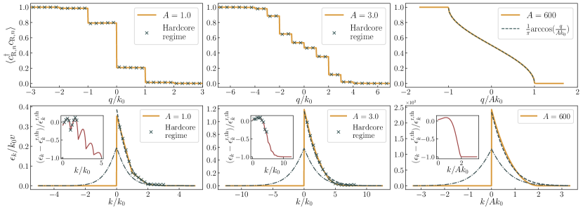
Figure 1: Relaxation of a single displaced phononic mode, characterized by $f_{R}(x)=A\cos(k_{0}x)$. Solid yellow lines are obtained by dynamical re-fermionization, i.e. Eqs. (17-18-Long time dynamics and relaxation.-21), in the thermodynamic limit $L\rightarrow\infty$. Top: Bethe-fermions occupations in the vicinity of the Fermi sea right-border. Bottom: Energy in each phononic mode after relaxation, $\epsilon_{k}=|k|v\langle A^{\dagger}_{R,n}A_{R,n}\rangle_{\infty}$, where $k=2n\pi/L$ (resp. $-2n\pi/L$) for right-movers (resp. left-movers). The dashed-dotted black lines is the results expected if the system would relax to a thermal equilibrium. Dashed line shows the distribution $\epsilon_{k}^{\rm r,th}$ corresponding to thermal redistribution of the initial energy within the right-movers phonons only and the insets highlight its difference with the dynamical refermionization results. Crosses are exact numerical results obtained in the limiting case of hard-core bosons, performed for 100 atoms (see text), using $k_{0}=5\times 2\pi/L$ in the left figure (resp. $k_{0}=2\times 2\pi/L$ in the central figure) for $A=1.0$ (resp. $A=3.0$), and the relaxed phonon population is computed in the fermionic diagonal ensemble. Those numerical results are performed for a lattice gas of 1000 sites, which represents faithfully the continuous gas only for small $k$.

Extracting the numbers $\beta_{I}$, or equivalently the expectations $\langle b^{\dagger}_{I}b^{\phantom{\dagger}}_{I}\rangle$ from the correlation functions Eqs. (14)-(15) which parameterize the initial phononic Gaussian state, is, generally speaking, an excruciating task. However, for an initial state in the low energy sector, only fermionic states close to the Fermi points are affected and calculation of $\langle b^{\dagger}_{I}b^{\phantom{\dagger}}_{I}\rangle$, which reduces to finding the distributions $\langle c^{\dagger}_{{\rm R},n}c^{\phantom{\dagger}}_{{\rm R},n}\rangle$, $\langle c^{\dagger}_{{\rm L},n}c^{\phantom{\dagger}}_{{\rm L},n}\rangle$, is much an easier task as it can be done by using bosonization.

To do this we concentrate on the right movers and introduce $G_{\mathrm{R}}(\xi)$ defined by

$$G_{\mathrm{R}}(\xi)=\frac{1}{L}\sum_{l}e^{-i2\pi l\xi/L}\langle c^{\dagger}_{\mathrm{R},l}c^{\phantom{\dagger}}_{\mathrm{R},l}\rangle\,.$$ (17)

which can be rewritten as the spatially averaged fermion two-point correlation function

$$G_{\mathrm{R}}(\xi)=(1/L)\int du\langle c^{\dagger}_{{\rm R}}(u+\xi/2)c^{\phantom{\dagger}}_{{\rm R}}(u-\xi/2)\rangle\,.$$ (18)

The crucial observation is that since $G_{R}$ is time-independent it can be evaluated using the initial state. Since the latter is a phononic Gaussian state, one can use Wick’s theorem for $\varphi_{\rm R}$ in Eq.(12) to evaluate of the two-point fermionic correlation function. One obtains, using $\langle\varphi_{\rm R}(x)\rangle_{0}=f_{\rm R}(x)$ and $\langle\varphi_{\rm R}(x)\varphi_{\rm R}(y)\rangle^{\rm conn.}_{0}=g_{\rm RR}(x,y)$,

$$\langle c^{\dagger}_{{\rm R}}(x)c^{\phantom{\dagger}}_{{\rm R}}(y)\rangle_{0}=\frac{1}{L}\exp\left[-i(f_{{\rm R}}\left(x\right)-f_{{\rm R}}\left(y\right))\right]$$

$$\times\exp\left[g_{\rm RR}\left(x,y\right)-\frac{1}{2}g_{\rm RR}^{\rm reg.}\left(x\right)-\frac{1}{2}g_{\rm RR}^{\rm reg.}\left(y\right)\right]$$ (19)

where $g_{{\rm RR}}^{\rm reg.}(x)\,=\,\lim_{y\to x}g_{{\rm RR}}(x,y)+\log(2\pi(y-x)/(iL))$ is independent of the short distance cutoff $\epsilon$. The function $G_{R}(\xi)$ is obtained by injecting Eq. (Long time dynamics and relaxation.) into Eq. (18). The population of the Bethe fermions, which entirely characterizes the state after relaxation, is then computed inverting Eq. (17). We dub this crucial intermediate result ‘dynamical refermionization’.

Consequence: relaxation of phonon population.

Mean values of products of phononic operators after relaxation are computed expressing them in terms of fermionic operators thanks to Eq.(10), and using Wick’s theorem, valid for the fermionic Gaussian density matrix Eq. (16). In particular, to compute $\langle J_{\rm R}(x)J_{\rm R}(y)\rangle_{\infty}$, we use the relation $J_{\rm R}(x)=(v\sqrt{K}/L)\sum_{l}\sum_{n\neq 0}e^{i2\pi nx/L}c^{\dagger}_{{\rm R},l+n}c^{\phantom{\dagger}}_{{\rm R},l}$, obtained injecting Eq. (10) into (4). This gives, for $x\neq y$,

$$\langle J_{\rm R}(x)J_{\rm R}(y)\rangle_{\infty}=-Kv^{2}G_{\rm R}(x-y)G_{\rm R}(y-x).$$ (20)

Also $\expectationvalue{J_{\mathrm{R}}(x)}_{\infty}=0$ due to translational invariance. The phonon population reads

$$\langle A^{\dagger}_{{\rm R},n}A_{{\rm R},n}\rangle_{\infty}=\frac{1}{n}\sum_{l}\langle c^{\dagger}_{{\rm R},l+n}c_{{\rm R},l+n}\rangle\left(1-\langle c^{\dagger}_{{\rm R},l}c_{{\rm R},l}\rangle\right).$$ (21)

Note that one should consider its weighted sum over a small but non-vanishing width in $k=2\pi n/L$, to ensure that the quantity is local so Eq. (16) applies.

Eqs. (20)-(21) constitute the main result of this paper. The translation-invariant case, Eq. (6), announced earlier, is obtained by using $f_{\rm R}(x)=0$, $g_{\rm RR}(x,y)=g(x-y)$, $g^{\mathrm{reg.}}_{\mathrm{RR}}(0)=0$. We stress that the relaxed state of the system is no longer Gaussian in terms of the phonons, so that higher order phononic correlation functions would require a separate calculation.

Example: application to the case of a single excited phononic mode.

Let us consider the situation where the initial state is obtained from the ground state by a displacement of an R-phonon: $f_{\rm R}(x)=A\cos(k_{0}x)$ with the amplitude $A$ and the wave-vector $k_{0}$, while keeping $g_{\rm RR}(x,y)$ equal to its ground-state value. Fig. 1 shows the Bethe fermion distribution obtained from dynamical refermionization, Eqs. (17),(18),(Long time dynamics and relaxation.). For small amplitudes $A$, one observes plateaus of width $k_{0}$ which reflect the quantization of phonons SM . As $A$ increases, more plateaus appear, and for large $A$ it becomes the smooth profile $\langle c_{{\rm R},n}^{\dagger}c_{{\rm R},n}\rangle=(1/\pi){\rm arccos}(2\pi n/(LAk_{0}))$ expected semiclassically SM . The bottom row of Fig. 1 shows the energy of each phononic mode after relaxation. The difference of the distributions of R and L-phonons is a strong signature of the non-thermal nature of the relaxed system. Within the space of R-phonons, redistribution of energy among phonons is found to be very efficient: the relaxed distribution is close, albeit not identical, to that expected for a thermal state. We compare the dynamical refermionization predictions to exact results in the asymptotic regime of hard-core bosons ($c\rightarrow\infty$): in this regime, the Hamiltonian in term of Bethe fermions is that of non-interacting fermions and the current operator $J_{R}$ is equal to that for the Bethe fermions, which enables exact calculations. The initial state is obtained as the ground state of the Hamiltonian $H+(Ak_{0}/\sqrt{K})\int dxJ_{\rm R}(x)\sin(k_{0}x)$. As seen in Fig. (1), results are in excellent agreement with the predictions of dynamical refermionization.

Experimental perspectives.

Our predictions can be tested in cold atom experiments, where initial out-of-equilibrium states can be generated in various ways. By quenching the longitudinal potential from a long-wavelength sinusoidal potential to a flat potential Cataldini et al. (2021), one produces displaced phononic states, corresponding to non vanishing functions $f_{\rm R}$, $f_{\rm L}$. A quench of the interaction strength will produce two-modes squeezed phononic states Schemmer et al. (2018), a situation which corresponds to $f_{\rm R}=f_{\rm L}=0$, but to modified functions $g_{{\rm R}{\rm R}}$, $g_{{\rm L}{\rm L}}$, $g_{\rm RL}$. Alternatively, modulating the coupling constant with time will parametrically excite only part of the phononic spectrum Jaskula et al. (2012). In the above scenarios the prepared initial state is symmetric under exchange of R and L-phonons. To break this symmetry, one could expose the gas to a potential $V(x)=V_{0}\cos(k_{0}x-vkt)$ for some short time duration: then only the R-phonons would be resonantly excited.

To probe the phonon distribution after relaxation, one possibility is to measure the in situ long-wavelength density fluctuations Esteve et al. (2006) and access $\delta\rho(x)=(J_{\rm R}(x)+J_{\rm L}(x))/v$, see Eq. (Sketch of the main result.). Alternatively, one can use the density ripple techniques to probe the long wavelength phase fluctuations Manz et al. (2010); Schemmer et al. (2018), whose gradient is the velocity field proportional to $J(x)=J_{\rm R}(x)-J_{\rm L}(x)$. The above methods however do not discriminate between right and left movers. In order to probe selectively R-phonons, one needs to probe the dynamics, for instance using sequences of non-destructive images Andrews et al. (1997).

At very long times, one expects integrability breaking perturbations to bring the system to a thermal equilibirum. However, such perturbations can be weak enough to have negligible effect during the relaxation time of the Lieb-Liniger phonons, as is observed experimentally in Ref. Cataldini et al. (2021) and modeled recently in Ref. Møller et al. (2022).

Interestingly, the occupation of Bethe fermions $\langle c^{\dagger}_{{\rm R},n}c_{{\rm R},n}\rangle$ —which, in this Letter, is used as an intermediate result — could also be measured experimentally. To measure it, one could first perform an adiabatic increase of the repulsion strength $c$, which preserves the distribution of Bethe fermions Bastianello et al. (2019), until the hard-core regime is reached. In this regime the distribution of Bethe fermions is the same as the rapidity distribution, which can be measured by a 1D expansion Wilson et al. (2020); Bouchoule and Dubail (2022).

Prospects.

This work calls for further investigations in several directions. First, one could investigate higher order functions of the chiral currents or of the phonons populations to show that the relaxed state is non Gaussian with respect to the phonons. Secondly, our predictions call for numerical studies of relaxation in the Lieb-Liniger model away from the strongly interacting regime. Finally, as discussed above, the predictions of this Letter are to be confirmed experimentally.

Appendix A Matrix element of density and current operators between two low-energy eigenstates of the Lieb-Liniger Hamiltonian

A.1 Density operator

Various formulas are available in the literature for form factors of the density operator $\delta\rho(x)$, see e.g. Slavnov (1989); Kozlowski (2011); Kozlowski et al. (2011); Kozlowski and Maillet (2015); De Nardis and Panfil (2015, 2018). Here we use formula (8) of Ref. De Nardis and Panfil (2018) as a starting point. That formula says that the matrix element between a Bethe state $\left|\psi\right>$ and another Bethe state $\left|\psi^{\prime}\right>$, multiplied by the system size $L$, vanishes in the thermodynamic limit, unless $\left|\psi^{\prime}\right>$ is obtained from $\left|\psi\right>$ by a single particle-hole excitation. In that case, if $p$ is the rapidity of the particle and $h$ is the rapidity of the hole, then the matrix element is

$$L\left|\left<\psi^{\prime}\right|\delta\rho(x)\left|\psi\right>\right|\underset{p\rightarrow h}{=}k^{\prime}(p)\left|\frac{\lambda_{0}-h}{\lambda_{0}-p}\right|^{\Delta\vartheta(F(\lambda_{0}|p)-F(\lambda_{0}|h))}$$ (22)

where $k(\lambda)$ is the dressed momentum as a function of the rapidity $\lambda$, $\lambda_{0}$ is the rapidity at the Fermi point, $\Delta\vartheta$ is the height of the discontinuity of the occupation ratio at the Fermi point (here, for the ground state, we simply have $\Delta\vartheta=1$), and $F(\lambda|\lambda^{\prime})$ is the backflow, see Ref. De Nardis and Panfil (2018). For low-energy excitations around the ground state, both $p$ and $h$ are very close to $\lambda_{0}$, so

$$L\left|\left<\psi^{\prime}\right|\delta\rho(x)\left|\psi\right>\right| \underset{p,h\rightarrow\lambda_{0}}{=} k^{\prime}(\lambda_{0})e^{{\partial_{\lambda^{\prime}}F(\lambda_{0}|\lambda^{\prime})_{|\lambda^{\prime}=\lambda_{0}}\,(p-h)\log\left|\frac{\lambda_{0}-h}{\lambda_{0}-p}\right|}}$$

$$= k^{\prime}(\lambda_{0})\left(1+O(|p-h|\log|p-h|)\right),$$

and the derivative of the dressed momentum at the Fermi rapidity is the square root of the Luttinger parameter, $k^{\prime}(\lambda_{0})=\sqrt{K}$ (see e.g. Ref. Korepin et al. (1997)). So, in the notations of our main text, we have that the matrix element of the Fourier mode $\delta\rho_{n}=\int_{0}^{L}e^{i2\pi nx/L}\delta\rho(x)dx$ between two low-energy Bethe states $\left|\psi_{1}\right>$, $\left|\psi_{2}\right>$ in the thermodynamic limit is

$$\left<\psi_{2}\right|\delta\rho_{n}\left|\psi_{1}\right>=$$ (23)

$$\sqrt{K}\left<\psi_{2}\right|\sum_{l\in\mathbb{Z}+\frac{1}{2}}c^{\dagger}_{{\rm R},n+l}c_{{\rm R},l}+\sum_{l\in\mathbb{Z}+\frac{1}{2}}c^{\dagger}_{{\rm L},n+l}c_{{\rm L},l}\left|\psi_{1}\right>,$$

up to corrections of order $O(\log L/L)$.

A.2 Current operator

A similar formula is obtained for the expectation value of the Fourier modes of the current operator, $J_{n}=\int_{0}^{L}e^{i\frac{2\pi nx}{L}}J(x)dx$. It follows from the one for the density operator, and from continuity equation. Indeed, using

$$\partial_{x}J(x)=-\partial_{t}\delta\rho(x)=-i[H,\delta\rho(x)]$$ (24)

one finds

$$-i\frac{2\pi n}{L}\left<\psi_{2}\right|J_{n}\left|\psi_{1}\right> = -i\left<\psi_{2}\right|[H,\delta\rho_{n}]\left|\psi_{1}\right>$$ (25)

$$= -i(E_{2}-E_{1})\left<\psi_{2}\right|\delta\rho_{n}\left|\psi_{1}\right>,$$

where $E_{1}$ and $E_{2}$ are the energies of the eigenstates $\left|\psi_{1}\right>$, $\left|\psi_{2}\right>$. According to the expression given in the main text, the difference between energies for a single particle-hole excitation of momentum $p-h=\frac{2\pi n}{L}$ is $E_{2}-E_{1}=\epsilon(p)-\epsilon(h)\simeq\frac{2\pi vn}{L}$. This, together with Eq. (23), gives the matrix element of the current operator in the thermodynamic limit,

$$\left<\psi_{2}\right|J_{n}\left|\psi_{1}\right>=$$ (26)

$$v\sqrt{K}\left<\psi_{2}\right|\sum_{l\in\mathbb{Z}+\frac{1}{2}}c^{\dagger}_{{\rm R},n+l}c_{{\rm R},l}-\sum_{l\in\mathbb{Z}+\frac{1}{2}}c^{\dagger}_{{\rm L},n+l}c_{{\rm L},l}\left|\psi_{1}\right>,$$

up to corrections of order $O(\log L/L)$. The matrix elements (23) and (26) then lead to formula (10) in the main text.

Appendix B Asymptotic behavior of the Bethe fermion distribution for a displaced phonon mode at $T=0$

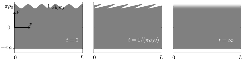
Figure 2: Illustration of dynamical refermionization in the semiclassical limit, when the number of phonons in the initial states is large. For simplicity we focus on the hard-core limit, where the dynamics of the bosons maps to the one of non-interacting fermions. Semiclassically, the fermions at zero temperature fill a region of phase space (grey area). In the initial state, this region is the set of all points $(x,p)$ with $0\leq x<L$ and $\pi\rho_{0}\leq p\leq\pi\rho_{0}-A_{0}k_{0}\sin(k_{0}x)$. Then, at later times $t$, all points in phase space get translated at the velocity $v(p)=p$. Consequently, the initial oscillations around the right Fermi point get deformed into waves that are more and more elongated in the $x$-direction. This results in thin layers of alternating empty/filled regions along the $p$-direction. At very long times, this layered structure can be locally averaged, resulting in a smooth distribution around the R-Fermi point. Although here we formulated the argument for the hard-core limit, it is easily adapted to the finite repulsion case using Generalized Hydrodynamics Castro-Alvaredo et al. (2016); Bertini et al. (2016), see in particular Doyon et al. (2017).

Let us consider the particular case of an initial state parameterized by (in this Appendix we set the sound velocity to $v=1$)

$$\left<J_{\rm R}(x)\right>_{0} = \frac{\sqrt{K}}{2\pi}\partial f_{\rm R}(x),$$ (27)

$$\left<J_{\rm R}(x)J_{\rm R}(y)\right>_{0}^{\rm conn.} = -\frac{(\frac{\sqrt{K}}{2\pi})^{2}}{[\frac{L}{\pi}\sin(\frac{\pi(x+i\epsilon-y)}{L})]^{2}},$$ (28)

This is a state obtained from the ground state, by displacing some of the R-phonons. Then the fermion two-point function in the initial state is

$$\langle c_{\rm R}^{\dagger}(x)c_{\rm R}(y)\rangle_{0}=\frac{i}{2\pi}\frac{e^{-if_{\rm R}(x)+if_{\rm R}(y)}}{\frac{L}{\pi}\sin(\frac{\pi(x-y+i\epsilon)}{L})},$$ (29)

and the occupation of the ${\rm R}$-fermions,

$$\left<c^{\dagger}_{{\rm R},n}c_{{\rm R},n}\right> = \int_{0}^{L}e^{i\frac{2\pi n}{L}v}\left<c_{\rm R}^{\dagger}(v/2)c_{\rm R}(-v/2)\right>dv.$$

B.1 Limiting cases

• Large number of phonons: $|f_{\rm R}(x)|\gg 1$. In that case $e^{if_{\rm R}(u+v/2)}$ oscillates very fast, and we can evaluate the integral by the stationary phase approximation. Because of the denominator in (29), the integral is dominated by the neighborhood of $v=x-y=0$, and we find

  $$\langle c^{\dagger}_{{\rm R},n}c_{{\rm R},n}\rangle \simeq \frac{1}{L}\int_{0}^{L}du\int_{-\infty}^{\infty}dv\frac{i}{2\pi}\frac{e^{i[\frac{2\pi n}{L}-\partial f_{\rm R}(u)]v}}{v+i\epsilon}$$ (30)

  $$= \frac{1}{L}\int_{0}^{L}du\leavevmode\nobreak\ \Theta(\partial f_{\rm R}(u)-\frac{2\pi n}{L}),$$ (31)

  where $\Theta(.)$ is the Heaviside step function. This is precisely what is expected from the geometric intuition illustrated in Fig. 2.

• Small density of phonons: $|f_{\rm R}(x)|\ll 1$. In that case we can simply expand the exponential in the numerator of (29),

  $$\langle c^{\dagger}_{{\rm R},n}c_{{\rm R},n}\rangle \simeq \frac{1}{L}\int_{0}^{L}du\int_{0}^{L}dv\leavevmode\nobreak\ e^{i\frac{2\pi n}{L}v}\frac{i}{2\pi}\frac{1-i[f_{\rm R}(u+v/2)-f_{\rm R}(u-v/2)]-\frac{1}{2}[f_{\rm R}(u+v/2)-f_{\rm R}(u-v/2)]^{2}}{\frac{L}{\pi}\sin(\frac{\pi v+i\epsilon}{L})}$$ (32)

  $$= \Theta(-n)-\frac{1}{2}\int_{0}^{L}dv\leavevmode\nobreak\ \frac{i}{2\pi}\frac{e^{i\frac{2\pi n}{L}v}}{\frac{L}{\pi}\sin(\frac{\pi v+i\epsilon}{L})}\left(\frac{1}{L}\int_{0}^{L}[f_{\rm R}(u+v/2)-f_{\rm R}(u-v/2)]^{2}du\right).$$

  The first order term in the expansion does not contribute because $\int[f_{\rm R}(u+v/2)-f_{\rm R}(u-v/2)]du=0$.

B.2 Special case: sinusoidal wave.

If we specialize to

$$f_{\rm R}(x)=A_{0}\cos(k_{0}x),$$ (33)

corresponding to a single phonon excited w.r.t the ground state, then formula (30) gives the fermion occupation

$$\langle c^{\dagger}_{{\rm R},n}c_{{\rm R},n}\rangle\simeq\frac{1}{\pi}{\rm arccos}\left(\frac{2\pi n/L}{A_{0}k_{0}}\right),$$ (34)

while formula (32) gives

$$\langle c^{\dagger}_{{\rm R},n}c_{{\rm R},n}\rangle \simeq \Theta(-n)-\frac{1}{2}\int_{0}^{L}dv\leavevmode\nobreak\ \frac{i}{2\pi}\frac{e^{i\frac{2\pi n}{L}v}}{\frac{L}{\pi}\sin(\frac{\pi v+i\epsilon}{L})}\left(A_{0}^{2}(1-\cos k_{0}v)\right)$$

$$\simeq \Theta(-n)-\frac{A_{0}^{2}}{2}\left(\Theta(-n)-\frac{1}{2}\Theta(k_{0}-\frac{2\pi n}{L})-\frac{1}{2}\Theta(-k_{0}-\frac{2\pi n}{L})\right).$$

The result (34) can be interpreted semi-classically, see Fig. 2. The result (B.2), on the other hand, where one observes the emergence of plateaux as in Fig. 1, is a consequence of phonon quantization.

References

- Slavnov (1989) N. A. Slavnov, Teoreticheskaya i Matematicheskaya Fizika 79, 232 (1989).
- Kozlowski (2011) K. K. Kozlowski, Journal of mathematical physics 52, 083302 (2011).
- Kozlowski et al. (2011) K. K. Kozlowski, J. M. Maillet, and N. A. Slavnov, Journal of Statistical Mechanics: Theory and Experiment 2011, P03018 (2011).
- Kozlowski and Maillet (2015) K. K. Kozlowski and J. M. Maillet, Journal of Physics A: Mathematical and Theoretical 48, 484004 (2015).
- De Nardis and Panfil (2015) J. De Nardis and M. Panfil, Journal of Statistical Mechanics: Theory and Experiment 2015, P02019 (2015).
- De Nardis and Panfil (2018) J. De Nardis and M. Panfil, Physical review letters 120, 217206 (2018).
- Korepin et al. (1997) V. E. Korepin, N. M. Bogoliubov, and A. G. Izergin, Quantum inverse scattering method and correlation functions, Vol. 3 (Cambridge university press, 1997).
- Castro-Alvaredo et al. (2016) O. A. Castro-Alvaredo, B. Doyon, and T. Yoshimura, Physical Review X 6, 041065 (2016).
- Bertini et al. (2016) B. Bertini, M. Collura, J. De Nardis, and M. Fagotti, Phys. Rev. Lett. 117, 207201 (2016).
- Doyon et al. (2017) B. Doyon, J. Dubail, R. Konik, and T. Yoshimura, Physical review letters 119, 195301 (2017).