Towards near-term quantum simulation of materials

Abstract

Simulation of materials is considered one of the most promising applications of quantum computers. On near-term hardware, the crucial constraint on simulations of real material models is the quantum circuit depth (and, to a lesser extent, the number of qubits required). The core of many quantum simulation algorithms, including time-dynamics and the variational quantum eigensolver under the Hamiltonian variational ansatz, is a layer of unitary evolutions by each local term in the Hamiltonian: a single Trotter step in time-dynamics simulation, or a single layer of VQE.

In this work we develop a new quantum algorithm design for materials modelling where this depth is independent of the system’s size. To achieve this, we take advantage of the locality of materials Hamiltonians in the Wannier single-particle electron basis and construct a tailored, multi-layer fermionic encoding that keeps the weight of Pauli operators appearing in the Hamiltonian independent of the system’s size. We analyse the circuit and measurement cost of this approach and present a compiler that is able to produce quantum circuit instructions for our method starting from density functional theory data, thus bridging from the physics description of a material to the quantum circuit needed to simulate it. The quantum circuits produced by our compiler are automatically optimised at multiple levels, not only at the circuit level but also incorporating optimisations derived from the physics of the specific target material. We present detailed numerical results for different materials spanning a wide structural and technological range. Our results demonstrate a reduction of many orders of magnitude in circuit depth over standard prior methods that do not consider the structure of the Hamiltonian.

For example, for Strontium Vanadate (SrVO₃), our results improve the resource requirements over standard quantum simulation algorithms from 864 to 180 qubits for a $3\times 3\times 3$ lattice, and the circuit depth of a single Trotter or variational layer from $7.5\times 10^{8}$ to depth $884$. Although these circuit depths are still beyond current hardware, our results show that realistic materials simulation may be feasible on quantum computers without necessarily requiring fully scalable, fault-tolerant quantum computers, providing quantum algorithm design incorporates deeper understanding of the specific target materials and applications.

1 Introduction

The race to demonstrate useful applications for near term quantum computers has begun in earnest, with quantum simulation being one of the leading candidates [georgescu14, bharti2021noisy]. Accurate simulations of complex materials yield valuable insight into their behaviour. This understanding serves to predict macroscopic properties and facilitates the rational design of materials with novel characteristics. The capability to understand and design characteristics in chemicals and materials is crucial for scientific, industrial, and commercial purposes, evidenced by the central role of classical simulation in guiding innovation in the multi-billion dollar chemical industry [icca_rep, Chem]. There are various challenges involved in the rational design of properties in novel materials, encompassing vastly different length and time scales; notably, fundamentally inefficient descriptions of electron–electron interactions hinder the ability to make predictions in the strong-coupling regime, where many relevant technological applications are expected to appear [quant_materials].

A quantum computer (QC) can simulate these correlated processes natively, by decomposing the quantum evolution into a sequence of elementary operations (i.e. a quantum circuit), applied to a specified quantum state. The state obtained from this procedure is then queried by measuring relevant quantities. Crucially, the advantage of this approach over direct classical simulation of the state vector appears for large enough systems (in terms of qubits and quantum circuit complexity), where the exponential growth of the Hilbert space outpaces state-of-the-art supercomputer capabilities [arute19].

Two main challenges pervade the noisy intermediate-scale quantum (NISQ) era of QCs. First, the number of physical qubits is restricted, although various hardware providers project that this will increase dramatically in the next decade [IBM, Google, IonQ]. The second challenge is to obtain gate fidelities sufficient to facilitate reliable circuits. Taken together, both capabilities are critical to the production of large quantum circuits, where error mitigation techniques can handle the noisy outcomes to generate meaningful signals beyond classical capabilities. Further developments will be required for quantum error correction and fault tolerance to become feasible, which themselves will allow for arbitrarily deep circuits.

These limitations on QCs constrain the types of algorithm that can in principle be implemented – and algorithms targeting near-term hardware should use all available strategies to minimize the required number of qubits and required circuit depth in order to meet these limitations. Materials’ simulation is well suited to this domain. Although the number of electrons in a large piece of material is of the order of Avogadro’s number, the regularity of the lattice restricts the behaviour of electrons, allowing us to concentrate the important degrees of freedom into a relevant active space, wherein the dominant mechanisms of interest lie. In doing so, we may minimise the number of qubits required to perform an accurate simulation. The periodic structure of materials also usually offers a great deal of symmetries, that can be leveraged to generate a compact representation of the Hamiltonian, lowering the number of interactions and ultimately the cost of implementing a circuit based on that Hamiltonian. Symmetries can also be used to mitigate errors in the measured signals, as already demonstrated experimentally [stanisic2021].

Materials’ systems also enjoy some useful properties. Band theory – namely the description of materials in terms of single-particle physics – is a well defined limit underlying the success of density functional theory (DFT). This limit provides a natural starting point for quantum state preparation, where one can initialize the system in the correct symmetry sector with an efficient quantum circuit. Moreover, using the single-particle state as a starting point has already been shown as a useful technique for error mitigation [montanaro2021_FLF]. Here, by training on the data obtained in a non-interacting instance, a map between the data obtained in the QC and the exact values can be inferred, and used to correct extracted data in the instances where classical simulations are not feasible. Similar error mitigation approaches are plausible for chemical systems, but have not yet been explored.

			Bands	Qubits	Depth
Material	Applications	Method
GaAs	Semiconductors [GaAs_semi], transistors [shur1987gaas], solar cells [Jun2013], spintronics [Okamoto2014]	This work	4	1120	7.9E+03
		Baseline estimate	18	4500	1.2E+11
H${}_{3}$S	Superconductors [Drozdov2015]	This work	7	1870	3.7E+04
		Baseline estimate	6	1500	4.0E+09
Li${}_{2}$CuO${}_{2}$	High-capacity battery cathode [Jing2017Li2CuO2]	This work	11	1024	8.4E+03
		Baseline estimate	11	990	1.1E+09
Si	Semiconductors [si_semi], solar cells [si_sc]	This work	4	1120	8.6E+03
		Baseline estimate	3	750	4.8E+08
SrVO${}_{3}$	Solar cells [srvo3_solar_cell], batteries [svo_anode, svo_cathode]	This work	3	180	8.8E+02
		Baseline estimate	16	864	7.5E+08

Table 1.1: Summary of resources needed to implement a single VQE layer that simulates the Hamiltonian of a material, without accounting for initial state preparation. The properties of the materials are listed in LABEL:tab:mat_props. Baseline estimates are based on standard methods available in the literature – namely employing the Jordan-Wigner transform in the Bloch basis – without considering the structure of the Hamiltonian (see LABEL:app:previous_method). For further details, see LABEL:sec:res_materials.

The description of electronic systems in digital quantum computers also presents particular challenges. While the most important components describing the physics of materials are electrons, most digital quantum computers operate with two-level systems, i.e. qubits. In order to properly account for fermion statistics and the Pauli principle, an algebraic mapping between fermions and qubits is needed. The usual mapping – the Jordan Wigner (JW) transform – can increase the cost of a computation by a multiplicative factor which scales according to the size of the system, outweighing the benefits yielded by preparing a local fermion Hamiltonian. Further, crystalline solids possess at least two natural bases for the single-particle electrons, the band (Bloch) basis, which represents electrons in momentum space, and the Wannier basis, which represents electrons in real space. Each single-particle basis affects the final cost of implementing a circuit differently, so we must establish stringent principles upon which we may choose between them.

In this work we take advantage of the interplay between single-particle bases, locality, symmetries, fermionic encodings, fermionic swap networks, and measurement strategies in order to develop novel, efficient algorithms for simulating materials’ systems. In doing so, we demonstrate a speed up of multiple orders of magnitude over standard methods, in a cost model assuming all-to-all hardware connectivity and cost 1 for each 2-qubit gate. Selected results appear in Table 1.1, where we compare the circuit depth obtained by our methods with a standard, generic method that does not exploit the structure of the Hamiltonian (see LABEL:app:previous_method for details). The materials analysed here represent a selection of systems whose behaviours are dominated by distinct underlying mechanisms: they span a minimal but wide structural, chemical, and technological range. Strontium vanadate (SrVO${}_{3}$) is a strongly correlated material that serves as a benchmark for post-DFT methods [Sheridan2019], gallium arsenide (GaAs) is a fairly well-understood material with many technological applications. Likewise, Si is the cornerstone material used in modern electronics [si_sc] and is also important in many other applications, such as solar technologies [si_sc]. Recently, hydrogen disulfide (H${}_{3}$S) has been found to host a high superconducting transition temperature at high pressures [Drozdov2015]. Finally, lithium copper oxide (Li${}_{2}$CuO${}_{2}$) is a material used in advanced lithium-ion battery technology [Jing2017Li2CuO2].

We present a unified resource estimate for quantum algorithms, namely VQE, and Time Dynamics Simulation (TDS), where a layer represents a single Trotter step or single Hamiltonian Variational Ansatz VQE layer in the overall evolution. The remainder of this text describes the numerous strategies employed to achieve these resource estimates.

1.1 Comparison with earlier works

Qubit and gate resources required for Trotterized Hamiltonian simulation algorithms of local Hamiltonians have recently been investigated by Kanno et al. [Kanno22]. Here, effective Hamiltonians of several unit cells of materials have been constructed starting from a classical description that accounts for the important chemistry of the active space [Imada10]. The resources to implement a single Trotter step are investigated on devices with nearest-neighbor connectivity in terms of CNOT and arbitrary single-qubit gates. They use a JW transform to encode the fermionic modes, and fermionic swaps [kivlichan18, OGorman19] to deal with the large operator weight of the encoded Pauli operators. This leads to a scaling of the gate count that is $O(N_{\rm cells}^{2})$ for a Hamiltonian defined in $N_{\rm cells}$ unit cells.

In comparison, our approach attains $O(N_{\rm cells})$ scaling of the number of gates, as the intercell interactions are implemented through ancillas in the compact encoding [derby2021compact]. This incurs a qubit overhead proportional to the number of unit cells. Importantly, considering that the main problem of current QCs is the presence of gate errors, our approach allows us to achieve a layer depth for single Trotter step that is independent of the size of the system, in stark contrast with the $O(N_{\rm cells}^{2/3})$ depth using JW (in a cubic system with nearest neighbour interactions).

Delgado et al. recently gave a detailed resource analysis of quantum algorithms for determining properties of battery materials, such as equilibrium voltages and thermal stability [delgado22]. They use a first quantisation approach with the plane wave basis and compute the cost of the quantum phase estimation algorithm. Considering one unit cell of the material Li${}_{2}$FeSiO${}_{4}$ with 156 electrons, these authors find a Toffoli gate cost of between $10^{11}$ and $10^{15}$ for quantum phase estimation, depending on the number of plane waves and level of accuracy required.

Counting the overall number of Toffoli or T gates is an appropriate approach to estimate complexity in the fault-tolerant regime, as this quantity directly determines the (very significant) overhead required for fault-tolerance. For near-term quantum computers, depending on the architecture, quantum circuit depth can be more appropriate, for several reasons. First, quantum computations are limited by decoherence, which sets an upper bound on the overall running time, as measured by circuit depth. Second, as errors can be seen as spreading out across a quantum circuit within a ‘‘lightcone’’, lower-depth circuits lead to improved localisation of errors. Third, as the circuit depth determines the running time, a lower-depth circuit executes more quickly.

Several other works have produced quantum algorithmic resource costs tailored for the fault tolerant era in molecular systems [PRXQuantum.2.030305, Su2021, kim2022] and the interacting electron gas (Jellium) [Babbush2018, Kivlichan2020improvedfault, Su2021nearlytight, McArdle2022].

2 Design strategy

The NISQ era is characterised by QCs operating without fault tolerance, so the depth of implementable quantum circuits is fixed by the error level present in the available device. Therefore the construction of compact circuits for simulation is crucial, as it can enable meaningful results (i.e., circuits where the accumulated error can be mitigated), as opposed to the random noise otherwise likely. Such constructions rely on two critical components: the physical instance being simulated, and an efficient decomposition of the physical information into layers of quantum gates. Our design strategy tackles these aspects in tandem.

The first step is to identify the relevant degrees of freedom (DoF) of the phenomena under investigation. This is not a sharp (or even well defined) procedure, but instead depends on the nature of the question being asked. For a given material, for example, studying electric transport at low temperatures involves different physical processes than the melting behaviour at high temperature. At a high level, this approach consists of choosing an active space, commonly discussed in chemistry and materials science [jensen2016book]. This active space can be seen as a distillation of the relevant DoF at a certain energy scale. Once the relevant DoF in the active space have been identified, their dynamics are constructed: these dynamics are governed by an effective Hamiltonian which describes their interactions.

Once this effective Hamiltonian has been obtained, a map between the physical and the logical DoF is required. Abstractly, this procedure maps interactions between the original DoF to qubit operations. In particular for fermions, the interplay between the structure of the Hamiltonian interactions and the fermionic encoding plays an important role in the ability to create compact circuits. At the end of this step a collection of Pauli operators is derived, comprising the qubit Hamiltonian $H_{Q}$.

Following this, the protocol implementing all the terms in the qubit Hamiltonian is computed. Here, the general approach that we use has the same structure as Trotterization of the evolution operator ${\rm exp}(iH_{Q}t)$. The structure of this step is indicative of the cost of finding a ground state via a VQE approach (in particular under the Hamiltonian variational ansatz [wecker15]), or TDS. This produces the circuit for a single Trotter step (or a single layer of VQE). Finally, we determine the measurement protocol that produces the minimum measurement overhead. Clearly, the decisions at each stage will have an effect on final cost of implementing all the qubit operators present in $H_{Q}$ through a quantum circuit. Hence we adopt a multi-tiered strategy for minimizing the cost of the quantum circuit, that we describe below in the context of materials simulations.

For the physics-based construction of the Hamiltonian of a material we adopt the Born-Oppenheimer approximation [Cederbaum_BO, Solyom2_book, Ashcroft_book], and concentrate on the quantum description of the electron DoF, including the nuclei as a classical background potential. While this approach is general enough to be used in chemistry and materials science, we note that including the quantum mechanical DoF of the nuclei is also possible within this framework. The existence of the periodic ionic potential is a distinctive feature of materials, which sets them apart from molecules. We use DFT for a low level exploration of the active space of materials, defined as an energy window around the Fermi level. Using this window containing the relevant DoF, we construct an effective Hamiltonian by classically computing its matrix elements.

We study two natural single-particle bases for the electrons: the Bloch basis, and the Wannier basis [Solyom2_book, Ashcroft_book]. The bands kept in the active space become modes in the unit cell, and the size of the material determines the number of unit cells. Due to the locality in real space achieved by the Wannier basis, a bespoke selection of bands allows us to construct a local Hamiltonian in real space, where the Coulomb interactions are localised, and the hopping range of electrons between unit cells does not scale with the system size. This local Hamiltonian defines a motif that can be used to tile a system of any size without increasing the depth, i.e. the number of layers, each containing many quantum gates.

To leverage the locality of the obtained fermion Hamiltonians, we introduce a novel fermionic encoding that uses the local structure of Coulomb interactions and hopping terms by hybridizing two existing encodings: the JW transform within a unit cell (where the majority of the electron-electron interactions are present), and the compact encoding [derby2021compact] between unit cells, where fewer interactions have to be considered, following from the locality of the fermion Hamiltonian. This comes at the cost of introducing further ancillary qubits. In order to deal with the existence of large weight operators along the JW line, we introduce an algorithm based on the use of fermionic swap operations (fswaps) [kivlichan18]. These operations can bring operators closer together along the JW line and minimise their weight, by relabelling the fermionic modes. This construction can be expanded to span structures other than single unit cells, depending on the connectivity graph of the Hamiltonian in question.

We invoke a cost model where all-to-all qubit interactions are available, arbitrary 2-qubit gates have cost 1 each, and 1-qubit gates are free (i.e. negligible). We hereby perform an in-depth analysis of the cost of implementing the most general terms allowed by symmetry, and the cost of performing fswaps to bring modes into an adjacent ordering within the JW string. Finally, we analyse the cost of executing a full VQE layer of the Hamiltonian $H_{Q}=\sum_{k}H_{k}$ given by $\prod_{k}e^{i\theta_{k}H_{k}}$, where $\set{\theta_{k}}$ is a set of variational parameters. Here $H_{Q}$ is obtained from a fermion representation in the Wannier bases, with different fermionic encodings. Additionally, we calculate the classical measurement overhead, i.e., we determine how many times a given circuit must be repeated to estimate an observable of interest, according to a series of measurement strategies.

We develop a tool to perform the necessary decomposition into layers of simultaneously implementable terms from a given Hamiltonian. This allows us to study different materials and model Hamiltonians, to understand their cost complexity, and to find a full decomposition into quantum circuits. The summary of the design strategy to optimise over circuit cost is shown in Fig. 2.1.

A self-contained exposition of the physics behind the construction of Hamiltonians is presented in Section 3. The role of symmetries, Wannier and Bloch functions, and efficient techniques to construct the matrix elements are discussed there.

In LABEL:sec:qubit_rep we introduce a hybrid fermionic encoding, and discuss its use in the context of materials’ simulation, where it represents an efficient fermion-to-qubit mapping. In LABEL:sec:vqe_alg we first concentrate on the quantum algorithm (VQE) itself and then discuss the decomposition of operators in terms of gates, initial state preparation, time evolution according to the material’s Hamiltonian, and measurement protocols. Combining these ideas, in LABEL:sec:compiler we discuss the design of our circuit compiler, which we go on to use in LABEL:sec:results to analyse the cost of running a single layer of VQE or a single Trotter step for TDS, in examples of increasing complexity.

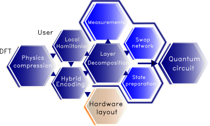
Figure 2.1: Summary of the strategy developed in this work to minimise circuit depth in the simulation of materials. Starting from a low level calculation based on DFT, we perform a compression of the physical information into relevant degrees of freedom. The locality of the interactions and the hardware layout determine the structure of the hybrid encoding. In order to minimise the circuit depth, the layer decomposition module determines the appropriate fswap networks, state preparation layers, and a measurement protocol. These elements constitute the quantum circuit that implements a layer of either VQE or TDS.

3 Effective description of the Hamiltonian

The full simulation of a physical system comprises infinitely many DoF, which makes it infeasible. This has never been a problem in domains where the relevant energy scale of the problem is restricted to a finite range. In this situation, the DoF at that scale are the ones that mostly contribute to the physical phenomena in question. For everyday applications, where most of the processes are controlled by the behaviour of the electron DoF in atoms, the Hamiltonian

$$H =\sum_{\sigma}\int d{\textbf{r}}\left[\frac{\hbar^{2}}{2m}|\nabla\hat{\psi}_{\sigma}(\textbf{r})|^{2}+\tilde{U}(\textbf{r})\hat{\psi}^{\dagger}_{\sigma}(\textbf{r})\hat{\psi}_{\sigma}(\textbf{r})\right]$$

$$+\frac{1}{2}\sum_{\sigma,\sigma^{\prime}}\int d\textbf{r}\int d\textbf{r}^{\prime}\hat{\psi}^{\dagger}_{\sigma}(\textbf{r})\hat{\psi}^{\dagger}_{\sigma^{\prime}}(\textbf{r}^{\prime})V(|\textbf{r}-\textbf{r}^{\prime}|)\hat{\psi}_{\sigma^{\prime}}(\textbf{r}^{\prime})\hat{\psi}_{\sigma}(\textbf{r})$$ (1)

describes all the possible non-relativistic physical systems in the absence of external magnetic fields. Here, $\hat{\psi}^{\dagger}_{\sigma}(\textbf{r})$ $(\hat{\psi}_{\sigma}(\textbf{r}))$ is an operator that creates (destroys) an electron at position r of spin $\sigma$. For the sake of notational simplicity, in what follows we will omit the hat when denoting operators. In Section 3, $V(|\textbf{r}-\textbf{r}^{\prime}|)$ is the distance-dependent repulsive potential between electrons. To derive explicit formulas, in what follows we will consider the screened Coulomb potential $V(|\textbf{r}-\textbf{r}^{\prime}|)=q_{e}(4\pi\epsilon_{0})^{-1}e^{-\mu|\textbf{r}-\textbf{r}^{\prime}|}/|\textbf{r}-\textbf{r}^{\prime}|$, with $\mu$ being the inverse screening length, but our results hold for any positive definite, central, and spin-independent potential. The constants $\hbar$, $m$, $q_{e}$ and $\epsilon_{0}$, are Planck’s constant, the electron mass, electron charge, and the vacuum permittivity of space respectively.

The abundant phenomena we observe in nature day-to-day is due, in part, to the structure of the potential $\tilde{U}(\textbf{r})$, which characterises the Coulomb potential produced by the positively charged nucleus of the atoms in the system.

In materials, the external potential created by the ions in the lattice heavily influences the electrons. Assuming a block of material is invariant under lattice translations $\textbf{R}_{n}$, the external potential satisfies $\tilde{U}({\textbf{r}}+{\textbf{R}_{n}})=\tilde{U}({\textbf{r}})$. A usual way of parameterising it is

$$\tilde{U}(\textbf{r})=\frac{q_{e}}{4\pi\epsilon_{0}}\sum_{I}\frac{Z_{I}}{|\textbf{r}-\textbf{r}_{I}|},$$ (2)

where $Z_{I}$ is the charge of the ions and $\textbf{r}_{I}$ is their position.

Starting from this scenario, in this section we discuss how the reduction of the Hamiltonian in Section 3 (which from now on we assume to represent a block of material, and thus lattice periodic) is performed, leading to a Hamiltonian over finitely many degrees of freedom and with an interaction structure that makes it amenable to simulation using shorter quantum circuits. As quantum simulation brings different communities together, we present a self contained discussion, revising familiar concepts to condensed matter physicists and materials scientists, but which may be not completely familiar to other communities.

3.1 General characteristics of fermion Hamiltonians

3.1.1 Structure of two and four fermion integrals

In this section we examine the general properties of the two- and four-fermion integrals occurring in the Hamiltonian of Section 3. We first expand the electron operator ${\psi}_{\sigma}(\textbf{r})$ in a basis of single-particle wavefunctions $\set{\phi_{\lambda}(\textbf{r})}$ as

$${\psi}_{\sigma}(\textbf{r})=\sum_{\lambda}\phi_{\lambda}(\textbf{r})c_{\lambda,\sigma},$$ (3)

where $\lambda$ represents the collection of all the particles’ quantum numbers but the spin, and $c_{\lambda,\sigma}$ ($c^{\dagger}_{\lambda,\sigma}$) is the annihilation (creation) operator for a fermion in the state $(\lambda,\sigma)$. In terms of the latter, Section 3 becomes

$$H=\sum_{\sigma}\sum_{\lambda_{1},\lambda_{2}}t_{\lambda_{1}\lambda_{2}}c^{\dagger}_{\lambda_{1},\sigma}c_{\lambda_{2},\sigma}+\sum_{\sigma,\sigma^{\prime}}\sum_{\lambda_{1},\lambda_{2},\lambda_{3},\lambda_{4}}V_{\lambda_{1}\lambda_{2}\lambda_{3}\lambda_{4}}c^{\dagger}_{\lambda_{1},\sigma}c^{\dagger}_{\lambda_{2},\sigma^{\prime}}c_{\lambda_{3},\sigma^{\prime}}c_{\lambda_{4},\sigma}.$$ (4)

Here, the hopping matrix is defined as

$$t_{\lambda_{1}\lambda_{2}}=\int d\textbf{r}\ \phi^{*}_{\lambda_{1}}(\textbf{r})\left[-\frac{\hbar^{2}\nabla^{2}}{2m}+\tilde{U}(\textbf{r})\right]\phi_{\lambda_{2}}(\textbf{r}),$$ (5)

while the Coulomb tensor is

$$V_{\lambda_{1}\lambda_{2}\lambda_{3}\lambda_{4}}=\frac{1}{2}\int d\textbf{r}\int d\textbf{r}^{\prime}\ \phi^{*}_{\lambda_{1}}(\textbf{r})\phi^{*}_{\lambda_{2}}(\textbf{r}^{\prime})V(|\textbf{r}-\textbf{r}^{\prime}|)\phi_{\lambda_{3}}(\textbf{r}^{\prime})\phi_{\lambda_{4}}(\textbf{r}).$$ (6)

In particular, both the hopping matrix and the Coulomb tensor are Hermitian, i.e., $t_{\lambda_{1}\lambda_{2}}=t^{*}_{\lambda_{2}\lambda_{1}}$ and $V_{\lambda_{1}\lambda_{2}\lambda_{3}\lambda_{4}}=V^{*}_{\lambda_{4}\lambda_{3}\lambda_{2}\lambda_{1}}$, where $a^{*}$ denotes the complex conjugate of $a$. From Eq. 6 it immediately follows that the Coulomb tensor obeys the index-swap symmetry $V_{\lambda_{1}\lambda_{2}\lambda_{3}\lambda_{4}}=V_{\lambda_{2}\lambda_{1}\lambda_{4}\lambda_{3}}$.

3.1.2 Cauchy-Schwarz inequality for the Coulomb tensor

Exploiting the fact that $V(|\textbf{r}-\textbf{r}^{\prime}|)$ is a real positive definite function, one can rewrite Eq. 6 in terms of an inner product. The latter can be defined in two possible ways. The first one is

$$V_{\lambda_{1}\lambda_{2}\lambda_{3}\lambda_{4}}\equiv\langle\rho_{\lambda_{1}\lambda_{2}},\rho_{\lambda_{4}\lambda_{3}}\rangle_{1}=\frac{1}{2}\int d\textbf{r}\int d\textbf{r}^{\prime}\ V(|\textbf{r}-\textbf{r}^{\prime}|)\rho^{*}_{\lambda_{1}\lambda_{2}}(\textbf{r},\textbf{r}^{\prime})\rho_{\lambda_{4}\lambda_{3}}(\textbf{r},\textbf{r}^{\prime}),$$ (7)

where $\rho_{\lambda_{i}\lambda_{j}}(\textbf{r},\textbf{r}^{\prime})\equiv\phi_{\lambda_{i}}(\textbf{r})\phi_{\lambda_{j}}(\textbf{r}^{\prime})$. Hence, the following inequality between the elements of the Coulomb tensor follows from the Cauchy-Schwarz inequality applied to Eq. 7

$$|V_{\lambda_{1}\lambda_{2}\lambda_{3}\lambda_{4}}|^{2}\leq|V_{\lambda_{1}\lambda_{2}\lambda_{2}\lambda_{1}}V_{\lambda_{4}\lambda_{3}\lambda_{3}\lambda_{4}}|.$$ (8)

On the other hand, another well-defined inner product can be introduced as

$$V_{\lambda_{1}\lambda_{2}\lambda_{3}\lambda_{4}}\equiv\langle\rho^{\prime}_{\lambda_{1}\lambda_{4}},\rho^{\prime}_{\lambda_{2}\lambda_{3}}\rangle_{2}=\frac{1}{2}\int d\textbf{r}\int d\textbf{r}^{\prime}\ V(|\textbf{r}-\textbf{r}^{\prime}|)\rho^{\prime*}_{\lambda_{1}\lambda_{4}}(\textbf{r})\rho^{\prime}_{\lambda_{3}\lambda_{2}}(\textbf{r}^{\prime}),$$ (9)

where $\rho^{\prime}_{\lambda_{i}\lambda_{j}}(\textbf{r})\equiv\phi_{\lambda_{i}}(\textbf{r})\phi^{*}_{\lambda_{j}}(\textbf{r})$. Similarly to the previous case, the Cauchy-Schwarz inequality associated with this inner product implies the following relation between the Coulomb tensor elements

$$|V_{\lambda_{1}\lambda_{2}\lambda_{3}\lambda_{4}}|^{2}\leq|V_{\lambda_{1}\lambda_{4}\lambda_{1}\lambda_{4}}V_{\lambda_{3}\lambda_{2}\lambda_{3}\lambda_{2}}|.$$ (10)

Eq. 8 and Eq. 10 can be exploited to obtain bounds on the Coulomb tensor coefficients, allowing one to truncate the elements smaller than a given threshold without having to directly compute them. This is usually very useful in reducing the classical computation needed to determine a quantum Hamiltonian.

3.2 Momentum-space single-particle bases

In this and the following sections we will introduce some of the most common single-particle bases to study condensed matter systems. As we will be discussing different bases for the same Hamiltonian, to avoid confusion, especially when these Hamiltonians are mapped into qubit operators, we will explicitly add a superscript to a Hamiltonian in a particular basis, each of which will be defined below. We will have:

• $H^{P}$: Hamiltonian Section 3 in the plane wave single-particle electron basis. The second quantized creation (annihilation) operators of momentum $k$ and spin $\sigma$ in this context are denoted by $c^{\dagger}_{k,\sigma}$ $(c_{k,\sigma})$. Choosing a lattice of discrete translations, the total momentum $k$ can always be decomposed in the lattice momentum k and reciprocal lattice vector G as $k=\textbf{k}+\textbf{G}$.

• $H^{B}$: Hamiltonian Section 3 in the Bloch-wave single-particle electron basis. The creation (annihilation) operators are $f^{\dagger}_{\textbf{k},n,\sigma}$ ($f_{\textbf{k},n,\sigma}$), with k the lattice momentum, $n$ the band index and $\sigma$ the spin.

• $H^{W}$: Hamiltonian Section 3 in the Wannier single-particle electron basis. The creation (annihilation) operators of band $n$ and spin $\sigma$ are $w^{\dagger}_{\textbf{R},n,\sigma}$ ($w_{\textbf{R},n,\sigma}$), where R is the lattice vector.

All single-particle basis operators (called generically $A_{j}$) satisfy the equal-time anti-commutation relations $\{A_{i},A^{\dagger}_{j}\}=\delta_{ij}$.

We begin with momentum-space bases, which fully exploit the translational invariance of crystalline solids. For more details see e.g., Refs. [Ashcroft_book, Solyom1_book]. In a material, atoms are arranged in a periodic structure (see Fig. 3.1) which is spanned by the lattice vectors $\textbf{R}_{a}$, $a=1,2,3$. The lattice points correspond to

$$\textbf{R}=n_{1}\textbf{R}_{1}+n_{2}\textbf{R}_{2}+n_{3}\textbf{R}_{3},$$ (11)

where $n_{a}\in\mathbb{Z}$. The lattice vector $\textbf{R}_{a}$ has length $R_{a}$. Translations $T_{\textbf{R}}$ along these lattice vectors leave the Hamiltonian $H$ invariant (assuming periodic boundary conditions). Consequently, we can block-diagonalize the Hamiltonian, and each block will correspond to a different eigenvalue of the translation operator. The Bloch Theorem allows us to find the simultaneous eigenfunctions of $T_{\textbf{R}}$ and $H$ [Ashcroft_book, Solyom1_book].

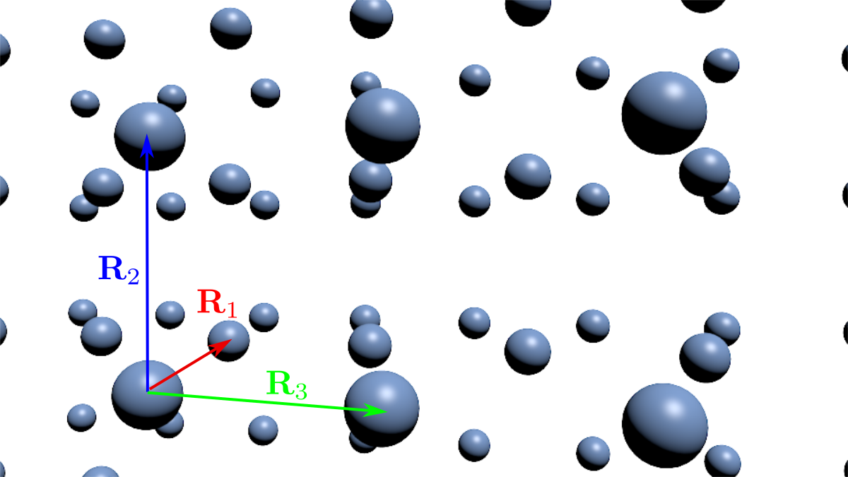
Figure 3.1: Simple Orthorhombic Bravais lattice, with its lattice vectors.

The translation operator $T_{\textbf{R}}$ forms an Abelian group, satisfying $T_{\textbf{R}}T_{\textbf{R}^{\prime}}=T_{{\textbf{R}}+{\textbf{R}^{\prime}}}$, with $T_{\textbf{0}}=1$. As $T$ should be represented by a unitary operator, in its diagonal basis it acts on the single-particle wavefunctions as

$$T_{\textbf{R}}\phi(\textbf{r})\equiv\phi({\textbf{r}}+{\textbf{R}})=e^{i{\textbf{k}}\cdot{\textbf{R}}}\phi({\textbf{r}}),$$ (12)

where the vector k is called the crystal momentum. In a periodic system with linear size $L_{a}=N_{a}R_{a}$ in each lattice vector direction, the periodic boundary conditions (Born-von Karman boundary conditions) $\psi({\textbf{r}}+N_{a}{\textbf{R}_{a}})=\psi({\textbf{r}})$ imply the quantization of the crystal momentum as

$${\textbf{k}}=\frac{n_{1}}{N_{1}}{\textbf{b}_{1}}+\frac{n_{2}}{N_{2}}{\textbf{b}_{2}}+\frac{n_{3}}{N_{3}}{\textbf{b}_{3}},$$ (13)

where the reciprocal lattice vectors ${\textbf{b}_{j}}$ satisfy ${\textbf{b}_{i}}\cdot{\textbf{R}_{j}}=2\pi\delta_{ij}$ and $n_{a}\in[0,N_{a}-1]$. The eigenstates of the translation operator $T_{\textbf{R}}$ can then be labelled by the triplet $n_{1},n_{2},n_{3}$, corresponding to a total of $N=N_{1}N_{2}N_{3}$ states. The total volume of the crystal is $V_{c}=N\Omega$, with $\Omega=|{\textbf{R}}_{1}\cdot({\textbf{R}}_{2}\times{\textbf{R}}_{3})|$ the volume of the unit cell. The relation between direct and reciprocal lattice is shown in Fig. 3.2.

Using Eq. 12, we can define

$$\phi_{\textbf{k}}({\textbf{r}})=e^{i{\textbf{k}}\cdot{\textbf{r}}}[e^{-i{\textbf{k}}\cdot{\textbf{r}}}\phi_{\textbf{k}}({\textbf{r}})]=e^{i{\textbf{k}}\cdot{\textbf{r}}}u_{\textbf{k}}({\textbf{r}}),$$ (14)

with $u_{\textbf{k}}({\textbf{r}}+{\textbf{R}})=u_{\textbf{k}}({\textbf{r}})$ a lattice periodic function. The single electron wavefunction $\phi_{\textbf{k}}({\textbf{r}})=e^{i{\textbf{k}}\cdot{\textbf{r}}}u_{\textbf{k}}({\textbf{r}})$ is called a Bloch wave [Ashcroft_book, Solyom2_book]. Since $u_{\textbf{k}}({\textbf{r}})$ is a lattice periodic function, it may be useful to expand it in Fourier series as

$$u_{\textbf{k}}(\textbf{r})=\sum_{\textbf{G}}u_{\textbf{k},\textbf{G}}e^{i\textbf{G}\cdot\textbf{r}},$$ (15)

where G is a reciprocal lattice vector ${\textbf{G}}=m_{1}{\textbf{b}_{1}}+m_{2}{\textbf{b}_{2}}+m_{3}{\textbf{b}_{3}}$, with $m_{i}\in\mathbb{Z}$, and to write the Bloch wave as

$$\phi_{\textbf{k}}(\textbf{r})=\sum_{\textbf{G}}u_{\textbf{k},\textbf{G}}e^{i(\textbf{k}+\textbf{G})\cdot\textbf{r}}.$$ (16)

3.2.1 Plane wave basis

A particularly simple choice for the functions $u_{\textbf{k}}(\textbf{r})$ is $u_{\textbf{k}}(\textbf{r})=N^{-1}\sum_{R}\delta(\textbf{r}-\textbf{R})$, with $\delta(\textbf{R})$ the Dirac delta function. This choice implies that all the Fourier coefficients $u_{\textbf{k},\textbf{G}}$ in Eq. 16 are set to 1 and, therefore, it corresponds to expanding the Bloch wave $\phi_{\textbf{k}}(\textbf{r})$ in the plane wave basis $\set{e^{i(\textbf{k}+\textbf{G})\cdot\textbf{r}}}$. An advantage of this basis is that plane waves for different momenta are orthogonal. The electron operator takes the form

$$\psi_{\sigma}(\textbf{r})=\frac{1}{\sqrt{V_{c}}}\sum_{{\textbf{k}},\textbf{G}}e^{i({\textbf{k}}+\textbf{G})\cdot{\textbf{r}}}c_{\textbf{k}+\textbf{G},\sigma},$$ (17)

where $c_{{\textbf{k}}+{\textbf{G}},\sigma}$ ($c^{\dagger}_{{\textbf{k}}+{\textbf{G}},\sigma}$) is the annihilation (creation) operator of an electron with momentum ${\textbf{k}}+{\textbf{G}}$ and spin $\sigma$. In the plane wave basis, the Hamiltonian of Eq. 4 becomes

$$H^{P}=\sum_{\textbf{k},\textbf{G},\textbf{G}^{\prime},\sigma}h_{\textbf{k},\textbf{G}-\textbf{G}^{\prime}}c^{\dagger}_{\textbf{k}+\textbf{G},\sigma}c_{\textbf{k}+\textbf{G}^{\prime},\sigma}+\sum_{\begin{subarray}{c}\textbf{k},\textbf{k}^{\prime},p\\ \textbf{G},\textbf{G}^{\prime},\sigma,\sigma^{\prime}\end{subarray}}V_{p}c^{\dagger}_{\textbf{k}+\textbf{G}+p,\sigma}c^{\dagger}_{\textbf{k}^{\prime}+\textbf{G}^{\prime}-p,\sigma^{\prime}}c_{\textbf{k}^{\prime}+\textbf{G}^{\prime},\sigma^{\prime}}c_{\textbf{k}+\textbf{G},\sigma},$$ (18)

where $h_{\textbf{k},\textbf{G}-\textbf{G}^{\prime}}=\left[\frac{|\hbar(\textbf{k}+\textbf{G})|^{2}}{2m}\delta_{\textbf{G},\textbf{G}^{\prime}}+U_{\textbf{G}-\textbf{G}^{\prime}}\right]$, $V_{p}=1/(2V_{c})\int d\textbf{r}e^{-ip\cdot\textbf{r}}V(|\textbf{r}|)$, and $p=\textbf{p}+\textbf{P}$ is the total momentum, with $\textbf{p}=\textbf{k}+\textbf{k}^{\prime}$ and $\textbf{P}=\textbf{G}+\textbf{G}^{\prime}$. $U_{\textbf{G}}$ is the Fourier component of the external lattice potential at reciprocal lattice vector G

$$\tilde{U}(\textbf{r})=\sum_{\textbf{G}}e^{i{\textbf{G}}\cdot\textbf{r}}U_{\textbf{G}}\quad\rightarrow\quad U_{\textbf{G}}=\frac{1}{\Omega}\int_{uc}d{\textbf{r}}e^{-i{\textbf{G}}\cdot\textbf{r}}\tilde{U}(\textbf{r}),$$ (19)

where the integral is over the unit cell. Using Eq. 2, we find

$$U_{\textbf{G}}=\frac{q_{e}}{\epsilon_{0}\Omega}\sum_{a}Z_{a}\frac{e^{i\textbf{r}_{a}\cdot\textbf{G}}}{|\textbf{G}|^{2}},\quad\mbox{for $\textbf{G}\neq 0$}\quad(U_{0}=0),$$ (20)

where the sum runs over the positions $\textbf{r}_{a}$ of the atoms in the unit cell (see Fig. 3.2).

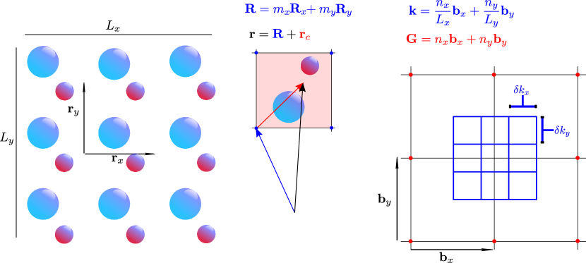
Figure 3.2: Direct and reciprocal lattice of a 2D square Bravais lattice. Left: Square Bravais lattice with two atoms per unit cell. The lattice vectors are $\textbf{r}_{x}$ and $\textbf{r}_{y}$ and the size of the system is $L_{x}$ and $L_{y}$. Middle: Every position r in the material can be decomposed in the position of the cell R and a position inside the cell $\textbf{r}_{c}$. Right: The reciprocal lattice (black grid) is unbounded. The finer $k$-mesh (blue lattice) represents the different lattice momentum states k. The system size determines the number of $k$ points and does not affect the reciprocal lattice.

3.2.2 Bloch wave basis

Going back to the Hamiltonian of Eq. 18, in the non-interacting limit we see that the lattice momentum k enters as a parameter,

$$H_{0}=\sum_{\textbf{k},\textbf{G},\textbf{G}^{\prime},\sigma}\left[\frac{|\hbar(\textbf{k}+\textbf{G})|^{2}}{2m}\delta_{\textbf{G},\textbf{G}^{\prime}}+U_{\textbf{G}-\textbf{G}^{\prime}}\right]c^{\dagger}_{\textbf{k}+\textbf{G},\sigma}c_{\textbf{k}+\textbf{G}^{\prime},\sigma}.$$ (21)

This implies that we can decompose the Hamiltonian in different crystal momentum blocks as $H=\sum_{\textbf{k}}H_{0}(\textbf{k})$ and solve an independent Schrödinger equation for each of them,

$$H_{0}(\textbf{k})|\Psi_{n}(\textbf{k})\rangle=\epsilon_{n}(\textbf{k})|\Psi_{n}(\textbf{k})\rangle,$$ (22)

with $|\Psi_{n}(\textbf{k})\rangle$ being a two-component spinor state. It is useful to define a particular zone of k values called the Brillouin zone, which corresponds to the Wigner-Seltz cell construction in reciprocal space, i.e., the locus of points k in the reciprocal space which is closer to $\textbf{G}=0$. The eigenvalues $\epsilon_{n}(\textbf{k})$ define the energy bands of the system.

The expansion of the non-interacting Hamiltonian in the basis defined by the momentum block eigenstates of Eq. 22, can be obtained by diagonalising $h_{\textbf{k},\textbf{G}-\textbf{G}^{\prime}}$ in Eq. 18,

$$H_{0}({\textbf{k}})\equiv\sum_{\textbf{G},\textbf{G}^{\prime},\sigma}h_{\textbf{k},\textbf{G}-\textbf{G}^{\prime}}c_{\textbf{k},\textbf{G},\sigma}^{\dagger}c_{\textbf{k},\textbf{G}^{\prime},\sigma}=\sum_{n,\sigma}\epsilon_{n}(\textbf{k})f_{\textbf{k},n,\sigma}^{\dagger}f_{\textbf{k},n,\sigma},$$ (23)

where $f_{\textbf{k},n,\sigma}=\sum_{\textbf{G}}S_{n,\textbf{G}}(\textbf{k},\sigma)c_{\textbf{k}+\textbf{G},\sigma}$ ($f^{\dagger}_{\textbf{k},n,\sigma}$) is the band fermion annihilation (creation) operator. Here, $S_{n,\textbf{G}}(\textbf{k},\sigma)$ is the unitary matrix that diagonalises $h$, i.e., $h_{\textbf{k},\textbf{G}-\textbf{G}^{\prime}}=\sum_{n}(S^{\dagger})_{\textbf{G},n}(\textbf{k},\sigma)\epsilon_{n}(\textbf{k})S_{n,\textbf{G}^{\prime}}(\textbf{k},\sigma)$. The index $n$ here denotes the band and takes the same number of values $|n|$ as the reciprocal lattice vectors G, i.e., $|n|=8G_{\rm max}^{3}$ in $D=3$ dimensions.

For a system with $\nu_{\rm el}$ electrons per unit cell (i.e., corresponding to a total of $\nu_{\rm el}\times N$ electrons), the system will have $\nu_{\rm el}$ occupied bands, as each band can accommodate $N$ states, which is the number of different lattice momentum values in the Brillouin zone (note that $\nu_{\rm el}$ can be a rational number, in which case there are $\lfloor\nu_{\rm el}\rfloor$ fully occupied bands and the last band $\lceil\nu_{\rm el}\rceil$ is partially occupied).

In real space, the non-interacting Hamiltonian corresponding to each momentum block is $H_{0}(\textbf{k})=\frac{\hbar^{2}}{2m}(\textbf{k}-i\nabla)^{2}+\tilde{U}(\textbf{r})$. The spin components of its eigenstates coincide with the periodic functions $u_{\textbf{k},n,\sigma}(\textbf{r})$ introduced in Eq. 14, i.e.,

$$H_{0}(\textbf{k})u_{\textbf{k},n,\sigma}(\textbf{r})=\epsilon_{n}(\textbf{k})u_{\textbf{k},n,\sigma}(\textbf{r}),$$ (24)

with the boundary condition $u_{\textbf{k}+\textbf{G},n,\sigma}(\textbf{r})=e^{-i\textbf{G}\cdot\textbf{r}}u_{\textbf{k},n,\sigma}(\textbf{r})$. Note that the functions $u_{\textbf{k},n,\sigma}(\textbf{r})$ are defined within the unit cell via $u_{\textbf{k},n,\sigma}(\textbf{r})=u_{\textbf{k},n,\sigma}(\textbf{r}_{c}+\textbf{R})=u_{\textbf{k},n,\sigma}(\textbf{r}_{c})$, where R is a lattice vector and $\textbf{r}_{c}$ is a vector with domain in the unit cell. By expanding $u_{\textbf{k},n,\sigma}(\textbf{r})$ in Eq. 24 in Fourier series one can verify that

$$u_{\textbf{k},n,\sigma}(\textbf{r})=\sum_{\textbf{G}}e^{i\textbf{G}\cdot\textbf{r}}S_{n,\textbf{G}}(\textbf{k},\sigma).$$ (25)

In the language of Section 3.1, what we have done so far corresponds to expanding the electron operator on a Bloch wave basis (also called band fermion basis) $\set{\phi_{\textbf{k},n,\sigma}(\textbf{r})}$, with $\phi_{\textbf{k},n,\sigma}(\textbf{r})=e^{i\textbf{k}\cdot\textbf{r}}u_{\textbf{k},n,\sigma}(\textbf{r})/\sqrt{V_{c}}$. In this basis, the full Hamiltonian is

$$H^{B}=\sum_{\textbf{k},n,\sigma}\epsilon_{n}(\textbf{k})f^{\dagger}_{\textbf{k},n,\sigma}f_{\textbf{k},n,\sigma}+\sum_{\sigma,\sigma^{\prime}}\sum_{\begin{subarray}{c}n_{1},n_{2},n_{3},n_{4}\\ \textbf{k},\textbf{q},\textbf{k}^{\prime}\end{subarray}}V_{n_{1}n_{2}n_{3}n_{4}}^{(\textbf{k},\textbf{k}^{\prime},\textbf{q})}f^{\dagger}_{\textbf{k}+\textbf{q},n_{1},\sigma}f^{\dagger}_{\textbf{k}^{\prime}-\textbf{q},n_{2},\sigma^{\prime}}f_{\textbf{k}^{\prime},n_{3},\sigma^{\prime}}f_{\textbf{k},n_{4},\sigma},$$ (26)

with Coulomb tensor coefficients

$$V_{n_{1}n_{2}n_{3}n_{4}}^{(\textbf{k},\textbf{k}^{\prime},\textbf{q})}=\sum_{\textbf{G},\textbf{K},\textbf{G}^{\prime}}V_{\textbf{q}+\textbf{K}}S_{n_{1},\textbf{G}+\textbf{K}}(\textbf{k}+\textbf{q},\sigma){S}_{n_{2},\textbf{G}^{\prime}-\textbf{K}}(\textbf{k}^{\prime}-\textbf{q},\sigma^{\prime})S^{*}_{n_{3},\textbf{G}^{\prime}}(\textbf{k}^{\prime},\sigma^{\prime})S^{*}_{n_{4},\textbf{G}}(\textbf{k},\sigma).$$ (27)

and $V_{\textbf{q}+\textbf{K}}$ defined after Eq. 18.

3.3 Real-space single-particle basis: Wannier functions

In Eq. 26, the quadratic part of the Hamiltonian is diagonal, but the electron-electron interaction is highly non-local. On the other hand, in a real-space coordinate basis (such as the one obtained by discretising the position operator r on a real-space grid), the electron-electron interaction is diagonal but non-local, while the kinetic term is not diagonal. To reduce the number of the relevant coefficients entering the Hamiltonian, one strategy is to look for a representation where both the hopping matrix and Coulomb tensor are not diagonal with respect to the single-particle basis, but as local (in real space) as possible. One convenient way to achieve this goal is to consider Wannier functions as the single-particle basis. The fermion annihilation operators associated with the latter are defined in [Marzari12] as

$$w_{\textbf{R},n,\sigma}=\sum_{\textbf{k},m}e^{i\textbf{k}\cdot\textbf{R}}U^{*}_{mn}(\textbf{k})f_{\textbf{k},m,\sigma}\rightarrow f_{\textbf{k},m,\sigma}=\frac{1}{N}\sum_{\textbf{R},n}e^{-i\textbf{k}\cdot\textbf{R}}U_{mn}(\textbf{k})w_{\textbf{R},n,\sigma},$$ (28)

where $U_{mn}(\textbf{k})$ is a unitary transformation representing the gauge freedom in the definition of the Bloch waves. In this basis, the Hamiltonian of Eq. 4 becomes

$$H^{W} =\sum_{\sigma}\sum_{\begin{subarray}{c}m,n\\ \textbf{R}_{1},\textbf{R}_{2}\end{subarray}}T(\textbf{R}_{1}-\textbf{R}_{2})_{mn}w_{\textbf{R}_{1},m,\sigma}^{\dagger}w_{\textbf{R}_{2},n,\sigma}$$

$$+\sum_{\sigma,\sigma^{\prime}}\sum_{\begin{subarray}{c}s,l,m,n\\ \textbf{R}_{1},\textbf{R}_{2},\textbf{R}_{3},\textbf{R}_{4}\end{subarray}}\tilde{V}^{(\textbf{R}_{1}\textbf{R}_{2},\textbf{R}_{3},\textbf{R}_{4})}_{slmn}w_{\textbf{R}_{1},s,\sigma}^{\dagger}w_{\textbf{R}_{2},l,\sigma^{\prime}}^{\dagger}w_{\textbf{R}_{3},m,\sigma^{\prime}}w_{\textbf{R}_{4},n,\sigma},$$ (29)

with the matrix elements

$$T(\textbf{R})_{mn} =\frac{1}{N^{2}}\sum_{\textbf{k}}e^{i\textbf{k}\cdot\textbf{R}}[U(\textbf{k})\epsilon(\textbf{k})U^{\dagger}(\textbf{k})]_{nm},$$ (30)

$$\tilde{V}_{slmn}^{(\textbf{R}_{1},\textbf{R}_{2},\textbf{R}_{3},\textbf{R}_{4})} =\frac{1}{N^{4}}\sum_{\begin{subarray}{c}n_{1}n_{2}n_{3}n_{4}\\ \textbf{k},\textbf{q},\textbf{k}^{\prime}\end{subarray}}V_{n_{1}n_{2}n_{3}n_{4}}^{(\textbf{k},\textbf{k}^{\prime},\textbf{q})}U^{*}_{n_{1}s}(\textbf{k}+\textbf{q})U^{*}_{n_{2}l}(\textbf{k}-\textbf{q})U_{n_{3}m}(\textbf{k}^{\prime})U_{n_{4}n}(\textbf{k})$$

$$\times e^{i\textbf{k}\cdot(\textbf{R}_{1}-\textbf{R}_{4})}e^{i\textbf{q}\cdot(\textbf{R}_{1}-\textbf{R}_{2})}e^{i\textbf{k}^{\prime}\cdot(\textbf{R}_{2}-\textbf{R}_{3})}.$$ (31)

The Wannier functions corresponding to the operators in Eq. 28 are

$$\mathcal{W}^{\textbf{R}}_{s,\sigma}(\textbf{r})=\mathcal{W}^{\textbf{0}}_{s,\sigma}(\textbf{r}-\textbf{R})=\sum_{\textbf{k},n}e^{-i\textbf{k}\cdot\textbf{R}}U_{ns}(\textbf{k})u_{\textbf{k},n,\sigma}(\textbf{r})e^{i\textbf{k}\cdot\textbf{r}}.$$ (32)

In terms of the latter, the matrix elements of the hopping matrix and the Coulomb tensor can expressed as

$$T(\textbf{R}_{1}-\textbf{R}_{2})_{mn} =\int d\textbf{r}\mathcal{W}^{\textbf{R}_{1}*}_{m,\sigma}(\textbf{r})\left[-\frac{\hbar^{2}\nabla^{2}}{2m}+\tilde{U}(\textbf{r})\right]\mathcal{W}^{\textbf{R}_{2}}_{n,\sigma}(\textbf{r}),$$ (33a)

$$\tilde{V}_{slmn}^{(\textbf{R}_{1},\textbf{R}_{2},\textbf{R}_{3},\textbf{R}_{4})} =\frac{1}{2}\int d\textbf{r}\int d\textbf{r}^{\prime}\mathcal{W}_{s,\sigma}^{\textbf{R}_{1}*}(\textbf{r})\mathcal{W}_{l,\sigma^{\prime}}^{\textbf{R}_{2}*}(\textbf{r}^{\prime})V(|\textbf{r}-\textbf{r}^{\prime}|)\mathcal{W}_{m,\sigma^{\prime}}^{\textbf{R}_{3}}(\textbf{r}^{\prime})\mathcal{W}_{n,\sigma}^{\textbf{R}_{4}}(\textbf{r}).$$ (33b)

The discrete translational invariance of the lattice allows us to rewrite the coefficients above as

$$T(\textbf{R})_{mn} =\int d\textbf{r}\mathcal{W}^{\textbf{R}}_{m,\sigma}(\textbf{r})\left[-\frac{\hbar^{2}\nabla^{2}}{2m}+\tilde{U}(\textbf{r})\right]\mathcal{W}^{\textbf{0}}_{n,\sigma}(\textbf{r}),$$ (34a)

$$\tilde{V}_{slmn}^{(\textbf{0},\textbf{R}_{2},\textbf{R}_{3},\textbf{R}_{4})} =\frac{1}{2}\int d\textbf{r}\int d\textbf{r}^{\prime}\mathcal{W}_{s,\sigma}^{\textbf{0}}(\textbf{r})\mathcal{W}_{l,\sigma^{\prime}}^{\textbf{R}_{2}}(\textbf{r}^{\prime})V(|\textbf{r}-\textbf{r}^{\prime}|)\mathcal{W}_{m,\sigma^{\prime}}^{\textbf{R}_{3}}(\textbf{r}^{\prime})\mathcal{W}_{n,\sigma}^{\textbf{R}_{4}}(\textbf{r}),$$ (34b)

with $\textbf{R}=\textbf{R}_{1}-\textbf{R}_{2}$.

Since the Coulomb tensor coefficients $\tilde{V}_{slmn}^{(\textbf{0},\textbf{R}_{2},\textbf{R}_{3},\textbf{R}_{4})}$ involves integrals over the real space, if the Wannier functions $\mathcal{W}_{s,\sigma}^{\textbf{R}}(\textbf{r})$ are localized around R, then the coefficients will decay fast for distant cells in the lattice. From the definition of the Wannier functions we have $\mathcal{W}^{\textbf{0}}_{s,\sigma}(\textbf{r})\equiv\sum_{\textbf{k}}v_{\textbf{k},{s},\sigma}(\textbf{r})e^{i\textbf{k}\cdot\textbf{r}}$, where $v_{\textbf{k},{s},\sigma}(\textbf{r})=\sum_{n}U_{ns}(\textbf{k})u_{\textbf{k},n,\sigma}(\textbf{r})$ are quasi-Bloch functions. This relation tells us that the quasi-Bloch functions and the Wannier functions are related by a Fourier transform. As discussed in LABEL:app:MLWFs, we can then use the analytical form of the quasi-Bloch functions $v_{\textbf{k},{s},\sigma}(\textbf{r})$ as a function of the crystal momentum k to show that