Superradiance and Subradiance in a Gas of Two-level Atoms

Abstract

Cooperative effects describe atomic ensembles with exchange of photonic excitations, such as dipole-dipole interactions. As a particular example, superradiance arises from spontaneous emission when this exchange leads to constructive interference of the emitted photons. Here, we introduce an integrated method for studying cooperative radiation in many-body systems. This method, which allows to study extended systems with arbitrarily large number of particles, can be formulated by an effective, nonlinear, two-atom master equation that describes the dynamics using a closed form which treats single- and many-body terms on an equal footing. We apply this method to a homogeneous gas of initially inverted two-level atoms, and demonstrate the appearance of both superradiance and subradiance, identifying a many-body coherence term as the source of these cooperative effects. We describe the many-body induced broadening – which is analytically found to scale with the optical depth of the system – and light shifts, and distinguish spontaneous effects from induced ones. In addition, we theoretically predict the time-dependence of subradiance, and the phase change of the radiated field during the cooperative decay.

I Introduction

Cooperative phenomena in many-body radiative systems result from the build-up of correlation among the radiators [1, 2]. The dipole-dipole interaction mediated by a shared electromagnetic field gives rise to the all-to-all coupling of the radiators, leading to a dramatically different behavior compared to that of independent ones. As first presented in the pioneering work by Dicke [1], superradiance results from the fact that a spontaneously emitted photon from one particle can stimulate emission from close-by neighbors (Fig. 1) [3, 4]. The emitted photons are phase coherent and therefore lead to an enhancement of radiated intensity (Fig. 2). Subradiance, on the contrary, results from the destructive interference between the emitted photons which suppresses radiation. These cooperative effects have been experimentally observed in various physical platforms, ranging from dense disordered atomic systems [5, 6, 7, 8, 9, 10, 11, 12] and ensembles of atoms in a cavity [13, 14, 15] to condensed matter systems such as two-dimensional materials [16] and quantum dots [17, 18]. While superradiance has been extensively studied due to its applications in laser techniques [19, 20] and the generation of spin-squeezing and entanglement [21, 22, 23, 24, 25], subradiant atomic modes offer promising avenues for sensing [26, 27], metrology [28] and light storage and retrieval [29, 30].

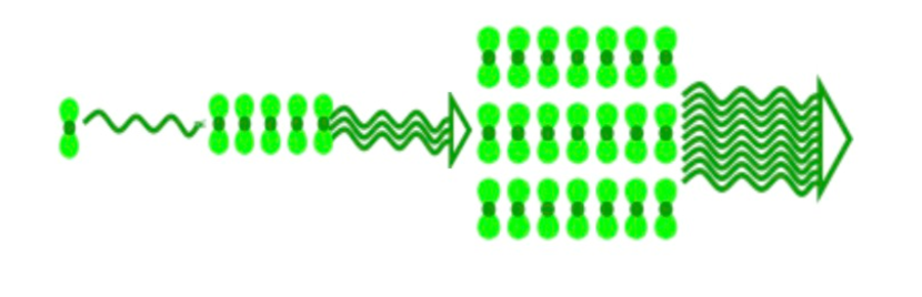
Figure 1: Visualization of superradiance. A photon emitted by one particle stimulates the close-by neighbors in turn, resulting in enhanced radiation.

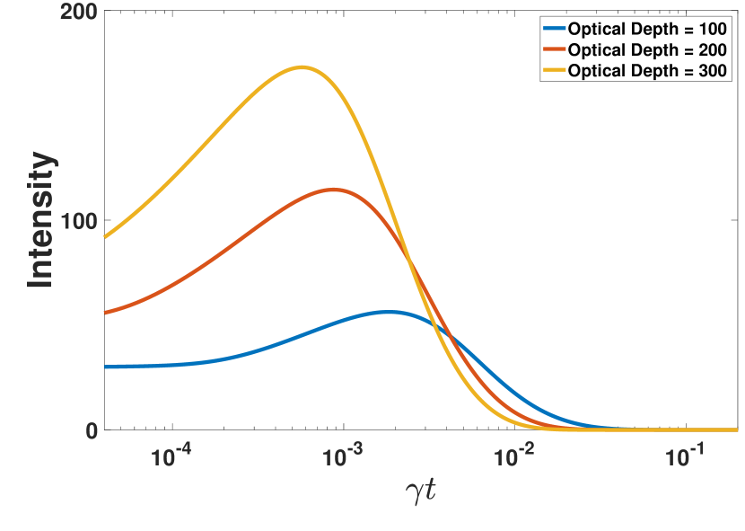
Figure 2: Radiated intensity (in arbitrary units) for superradiance with different optical depths of the sample, plotted with a dimensionless time scale, where $\gamma$ is the vacuum spontaneous decay rate.

Due to the interacting many-body nature of the problem, the dimensionality of the Hilbert space for an ensemble with $N$ particles grows exponentially as $2^{N}$, making theoretical approaches and numerical calculations challenging. Efforts have been made to reduce the complexity of the problem, including the case where all atoms are assumed to be within a volume of sidelength much smaller than the transition wavelength such that the system is described by the symmetric Dicke states [1, 2, 31, 32, 33]. Other methods rely on classical treatment [34, 35], restricting the system to singly-excited states [36, 37, 38, 39, 40, 41, 42], or considering ensembles with a small number of particles such that quantum Monte-Carlo wave function techniques can be applied [43, 44, 45]. The methods above reduce the full Hilbert space to a low-dimensional, relevant subspace and therefore make the problem feasible to solve, at the expense of compromising its applicability to systems with certain prerequisites. Recent studies exploit the system’s behavior at the initial time to predict the universal properties of superradiance for inverted ensembles with large number of atoms [46, 47]. While these formalisms do not require to solve the full time evolution of the system, they provide no information about the magnitude of the superradiant burst or the late time dynamics of the atomic ensemble.

In addition, there has been a large number of experimental demonstrations recently, such as those in Refs. [48, 49, 50, 51, 52], which can, as an overall sample of experimental results, only be confirmed theoretically by a comprehensive treatment of large-scale and long-time theoretical treatment.

In this article, we propose an integrated method to study correlated systems that exhibit cooperative phenomena such as superradiance and subradiance. Our goal is to obtain an effective description of a system with a large particle number, whose degrees of freedom are reduced to a solvable level. Additionally, this description does still preserve the many-body nature of the problem, including interactions, arising from quantum correlations. For that, we follow the idea of a mean-field-plus-second-order-correlations approach by tracing out the electromagnetic field and all but two atoms. As a result, we obtain the dynamics of the two remaining probe atoms, which reveal the cooperative behavior of arbitrarily large systems. As opposed to other treatments, the present formalism also reveals the analytical dependencies of the emission properties on the parameters of the system, such as the optical depth, the particle density and the magnitude of the external field.

Our formalism can be briefly outlined as follows: (i) we write down the full Hamiltonian of the system, which describes the atoms interacting with a shared quantized field and a classical driving field [Eq. (1)]. The Hamiltonian is then divided into two parts: an interaction term $V$, which consists of the interaction of two random probe atoms with the electromagnetic field, and $H_{0}$, which includes the interaction of the field with all the remaining atoms. (ii) We trace out the quantum field and the non-probe atoms, such that the dynamics effectively results from an atom-atom interaction and the degrees of freedom are dramatically reduced. This effective atom-atom interaction takes into account multiple scattering of photons to any order. (iii) We then develop a self-consistent formalism (see Fig. 3) in which the effective description of the full atomic ensemble is given by an average over all possible choices of probe atoms. (iv) This finally results in a nonlinear two-atom master equation of Lindblad form that captures the dynamics of the whole system.

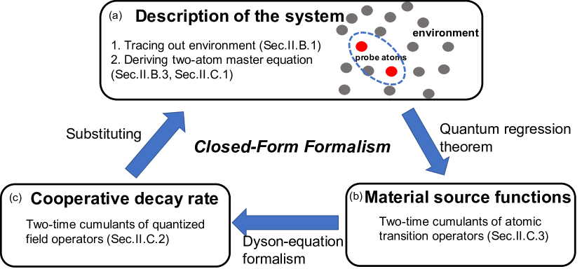
Figure 3: Schematic diagram of the closed form formalism.

In this article, we focus on the deceptively simple example of a homogeneous gas of two-level atoms and obtain the time-evolution of an initially fully inverted system. By calculating the radiated intensity and the off-diagonal coherence of the density matrix, we find a superradiant outburst at early times and subradiant emission immediately afterwards. The non-zero coherence shows that these are indeed cooperative effects. At late times, radiation trapping emerges [53], a regime characterized by a slowdown of emission in the absence of atomic coherences. Additionally, we demonstrate that observables such as the cooperative decay rate and the emission linewidth scale with the optical depth of the system. Finally, we investigate the slow decay in the subradiant regime, as well as the phase change of the radiated field during the cooperative decay.

II Method

The treatment in this section of the paper is a generalization and expansion of the method presented in Ref. [54], with the comprehensive formalism that is applicable to the presence of an external driving field, as well as an arbitrary geometry and particle distribution. It is worthwhile noting that the system does not needs to be small compared to the transition wavelength. Our treatment is valid as long as the time scale of cooperative decay $\tau_{coop}$ is longer than the propagation time of the radiation through the media $l/c$, where $l$ is the size of the sample, and $c$ is the speed of light .

II.1 Model

We consider an ensemble of $N$ two-level atoms that interact via a quantized electric field. We distinguish two probe atoms from the system, which are labeled as “1” and “2”. With the dipole approximation, the full Hamiltonian of the system is given by

$$H=H_{0}+V$$ (1)

where

$$H_{0} = H_{atom,free}+H_{field,free}-\sum_{i\neq 1,2}\vec{p}_{i}\cdot(\vec{\cal E}_{i}+\vec{E}_{i})$$

$$V = -\sum_{i=1,2}\vec{p}_{i}\cdot(\vec{\cal E}_{i}+\vec{E}_{i})$$

$H_{atom,free}\equiv\sum_{i}H_{atom,free}^{i}$ and $H_{field,free}$ are the free Hamiltonian for the atoms and quantized field, respectively. Here, $\vec{E}_{i}$ is the quantized field operator at the position of the $i$-th atom, $\vec{p}_{i}$ is the dipole operator of the $i$-th atom, and $\vec{\cal E}_{i}$ is the external classical driving field. Note that the spatial dependence of these quantities is implicitly included in the index $i$. The interaction term $V$ only includes the interaction between the probe atoms and the field, and all the atomic dipole operators couple to the radiation field at their own location.

Using the Keldysh formalism (see Ref.[56] and Appendix A), the dynamics of the full system are described by a time-evolution operator defined on the Schwinger-Keldysh contour $\cal C$.

$$S_{\cal C}\;\equiv\;{\cal T}_{\cal C}e^{-\frac{i}{\hbar}\int\limits_{\cal C}d\check{\tau}\,V^{I}(\check{\tau})}$$ (2)

where $V^{I}(\check{\tau})$ is the interaction term $V$ in the interaction picture and the check mark on the time variable denotes a time on the Keldysh contour. Note that $V^{I}(\check{\tau})$ contains the $\vec{E}_{i}$-term and therefore includes the effect of all the atoms. Each physical time $\tau$ corresponds to two times on the contour, $\check{\tau}=\tau_{+}$ on the upper branch and $\check{\tau}=\tau_{-}$ on the lower branch. ${\cal T}_{\cal C}$ is the time-ordering operator on the Keldysh contour defined as follows: it is the ordinary time-ordering operator (${\cal T}$) on the upper branch, and the inverse time-ordering operator (${\cal T}^{-1}$) on the lower branch. Additionally, terms that have time arguments on the lower branch are always ordered to the left, while terms on the upper branch are ordered to the right.

The state of the full system is described by a density matrix that includes the degrees of freedom of the $N$ atoms and the quantized field. Rewriting $\rho_{\alpha\beta}={\rm Tr}(\rho\left|\beta\right\rangle\!\!\left\langle\alpha\right|)$ in the interaction picture and defining the initial state $\rho_{0}\equiv\rho(t\!\to\!-\infty)$, the matrix elements can be written as (see Appendix A)

$$\rho_{\alpha\beta}(t)={\rm Tr}\left(\rho_{0}{\cal T}_{\cal C}{\cal S}_{\cal C}P_{\beta\alpha}^{I}(t)\right)\equiv\left\langle{\cal T}_{\cal C}{\cal S}_{\cal C}P_{\beta\alpha}^{I}(t)\right\rangle_{0}$$ (3)

II.2 Master Equation of an Effective Two-atom System

II.2.1 Tracing out the Environment

So far the model has been built upon an $N$-atom ensemble and the dimension of the density matrix in Eq. (3) is, in principle, $2^{N}\times$ the number of field modes. The exponential increase of its dimensionality make it unfeasible for a large particle number. We hereby follow the idea of a mean-field approach by looking into two probe atoms, and treating the rest of $(N-2)$ atoms and the field as the environment (denoted by the subscript $E$).

We define the effective time-evolution operator for the two-atom system by taking the average with respect to the environment

$${\cal S}^{\rm eff}_{\cal C}\equiv\left\langle{\cal S}_{\cal C}\right\rangle_{E}=\left\langle{\cal T}_{\cal C}{\rm exp}\left\{-\frac{i}{\hbar}\int_{\cal C}d\check{\tau}V^{I}(\check{\tau})\right\}\right\rangle_{E}$$ (4)

Using a generalized cumulant expansion method for the operators (see Appendix B), Eq. (4) can be further expressed as

$${\cal S}^{\rm eff}_{\cal C} = {\rm exp}\bigg{\{}\sum_{n=1}^{\infty}\frac{1}{n!}\left(-\frac{i}{\hbar}\right)^{n}\int...\int_{\cal C}d\check{\tau}_{1}...d\check{\tau}_{n}$$ (5)

$$\times\left\langle\!\left\langle{\cal T}_{\cal C}V^{I}(\check{\tau}_{1})...V^{I}(\check{\tau}_{n})\right\rangle\!\right\rangle_{E}\bigg{\}}$$

where $\left\langle\!\left\langle{\cal T}_{\cal C}V^{I}(\check{\tau}_{1})...V^{I}(\check{\tau}_{n})\right\rangle\!\right\rangle_{E}$ is the $n$-th order cumulant. Note that each of the cumulants is assigned with a time-ordering operator, such that the $V^{I}$ terms are ordered according to the branches that $\check{\tau}_{1}...\check{\tau}_{n}$ sit on. We further assume a Gaussian form for the radiation field, that is, only cumulants up to the second-order are kept . The resulting two-atom density matrix is a $4\times 4$ matrix

$$\tilde{\rho}_{\alpha\beta}(t) = \left\langle{\cal T}_{\cal C}{\cal S}^{\rm eff}_{\cal C}P^{I}_{\beta\alpha}(t)\right\rangle_{0}$$ (6)

where each of the subscripts $\alpha$ and $\beta$ represent a bare two-atom eigenstates $\alpha,\beta\in$ {gg,ge,eg,ee}.

II.2.2 Rotating Wave Approximation

In this section, we express the cumulants in terms of atomic dipole operators and quantized field operators. Note that all time-dependent operators in this section are in the interaction picture and that we drop the superscript to simplify the notation. We first separate the dipole and the fields into positive and negative frequency components

$$p_{i\mu}(\tau) = p_{i\mu}^{+}(\tau)e^{-i\omega_{a}\tau}+p_{i\mu}^{-}(\tau)e^{i\omega_{a}\tau}$$

$$E_{i\mu}(\tau) = E_{i\mu}^{+}(\tau)e^{-i\omega_{l}\tau}+E_{i\mu}^{-}(\tau)e^{i\omega_{l}\tau}$$

$${\cal E}_{i\mu}(\tau) = {\cal E}_{i\mu}^{+}(\tau)e^{-i\omega_{c}\tau}+{\cal E}_{i\mu}^{-}(\tau)e^{i\omega_{c}\tau}$$

where $i=1,2$ is the index for the probe atom and $\mu=x,y,z$ are the spatial components. Note that $p_{i\mu}$ and $E_{i\mu}$ are operators, while the classical driving field ${\cal E}_{i\mu}$ is a complex number. The negative (positive) frequency component of the dipole operator is associated with the atomic raising (lowering) operator,

$$p_{i\mu}^{+}(t) = \wp_{\mu}\sigma_{i\mu}(t)$$ (7)

$$p_{i\mu}^{-}(t) = \wp_{\mu}\sigma_{i\mu}^{\dagger}(t)$$ (8)

where $\wp_{\mu}$ is the dipole matrix element for polarization $\mu$ and $\sigma_{i\mu}=\left|g\right\rangle_{i\mu}\!\!\left\langle e\right|$.

Using the rotating wave approximation, we obtain the first-order cumulant

$$\left\langle\!\left\langle V(\check{\tau})\right\rangle\!\right\rangle = \left\langle V(\check{\tau})\right\rangle$$

$$= -\sum_{i,\mu}\left(p^{+}_{i\mu}(\check{\tau}){\cal E}^{-}_{L,i\mu}(\check{\tau})+p^{-}_{i\mu}(\check{\tau}){\cal E}^{+}_{L,i\mu}(\check{\tau})\right)$$

where we have defined the Lorentz-Lorenz local field [58, 59]

$${\cal E}_{L,i\mu}^{\pm}\;\equiv\;{\cal E}_{i\mu}^{\pm}+\langle E_{i\mu}^{\pm}\rangle$$ (9)

The second-order term is calculated as follows

$$\left\langle\!\left\langle{\cal T}_{\cal C}V(\check{\tau}_{1})V(\check{\tau}_{2})\right\rangle\!\right\rangle\;=$$

$$= \sum_{i\mu,j\nu}\left\langle\!\left\langle{\cal T}_{\cal C}\;p_{i\mu}(\check{\tau}_{1})E_{i\mu}(\check{\tau}_{1})p_{j\nu}(\check{\tau}_{2})E_{j\nu}(\check{\tau}_{2})\right\rangle\!\right\rangle$$

$$= \sum_{i\mu,j\nu}\{p^{+}_{i\mu}(\check{\tau}_{1})\left\langle\!\left\langle{\cal T}_{\cal C}E^{-}_{i\mu}(\check{\tau}_{1})E^{+}_{j\nu}(\check{\tau}_{2})\right\rangle\!\right\rangle p^{-}_{j\nu}(\check{\tau}_{2})e^{-i\omega(\check{\tau}_{1}-\check{\tau}_{2})}$$

$$+p^{-}_{i\mu}(\check{\tau}_{1})\left\langle\!\left\langle{\cal T}_{\cal C}E^{+}_{i\mu}(\check{\tau}_{1})E^{-}_{j\nu}(\check{\tau}_{2})\right\rangle\!\right\rangle p^{+}_{j\nu}(\check{\tau}_{2})e^{i\omega(\check{\tau}_{1}-\check{\tau}_{2})}\}$$

where $\omega=\omega_{a}-\omega_{l}$ is the detuning between atomic frequency and light frequency. In the first step, all terms with classical field $\cal E$ vanish in the cumulant. In the second step, the dipole operators are moved outside the cumulants, since the average does not involve the probe atoms. Under the rotating-wave approximation, the fast oscillating terms are dropped. Note that we explicitly write the ${\cal T}_{\cal C}$ in the cumulant.

We further define the following quantities

$$D_{i\mu,j\nu}^{\pm\pm} \equiv\left\langle\!\left\langle{\cal T}_{\cal C}E^{-}_{i\mu}(\check{\tau}_{1\pm})E^{+}_{j\nu}(\check{\tau}_{2\pm})\right\rangle\!\right\rangle$$ (11a)

$$C_{i\mu,j\nu}^{\pm\pm} \equiv\left\langle\!\left\langle{\cal T}_{\cal C}E^{+}_{i\mu}(\check{\tau}_{1\pm})E^{-}_{j\nu}(\check{\tau}_{2\pm})\right\rangle\!\right\rangle$$ (11b)

where the double superscript of $D$ and $C$ stands for the branches of $\check{\tau}_{1}$ and $\check{\tau}_{2}$. $D$ stands for terms like $\left\langle\!\left\langle{\cal T}_{\cal C}E^{-}E^{+}\right\rangle\!\right\rangle$, while $C$ is for $\left\langle\!\left\langle{\cal T}_{\cal C}E^{+}E^{-}\right\rangle\!\right\rangle$. Note that the time-ordering operator ${\cal T}_{\cal C}$ will simplify once the branches of the time variables are determined.

II.2.3 Derivation of the Master Equation

Taking the time derivative on both sides of Eq. (6) results in the master equation

$$\dot{\rho}_{\alpha\beta}(t)=\left\langle{\cal T}_{\cal C}\dot{\cal S}^{\rm eff}_{\cal C}P^{I}_{\beta\alpha}(t)\right\rangle+\left\langle{\cal T}_{\cal C}{\cal S}^{\rm eff}_{\cal C}\dot{P}^{I}_{\beta\alpha}(t)\right\rangle$$ (12)

where we have omitted the tilde over the reduced density matrix. The second term of Eq. (12) gives rise to the dynamics corresponding to the free Hamiltonian $H_{0}$

$$\left\langle{\cal T}_{\cal C}{\cal S}^{\rm eff}_{\cal C}\dot{P}^{I}_{\beta\alpha}(t)\right\rangle = -\frac{i}{\hbar}\left\langle{\cal T}_{\cal C}{\cal S}^{\rm eff}_{\cal C}\left[P^{I}_{\beta\alpha}(t),H_{0}\right]\right\rangle$$

$$= -\frac{i}{\hbar}\left\langle\alpha\right|\left[H_{0},\rho(t)\right]\left|\beta\right\rangle$$

The first term of Eq. (12) includes all the non-trivial effects arising from second-order correlations. Defining the term

$$P\equiv\sum_{n=1}^{\infty}\frac{1}{n!}\left(-\frac{i}{\hbar}\right)^{n}\int...\int_{\cal C}d\check{\tau}_{1}...d\check{\tau}_{n}\left\langle\!\left\langle{\cal T}_{\cal C}V^{I}(\check{\tau}_{1})...V^{I}(\check{\tau}_{n})\right\rangle\!\right\rangle_{E}$$ (13)

one can formally write

$$\dot{\cal S}^{\rm eff}_{\cal C}=\frac{d}{dt}{\cal T}_{\cal C}e^{P}={\cal T}_{\cal C}\left(\frac{d}{dt}P\right)e^{P}={\cal T}_{\cal C}\frac{d}{dt}\left(-\frac{i}{\hbar}\int_{\cal C}d\check{\tau}_{1}\left\langle V^{I}(\check{\tau}_{1})\right\rangle-\frac{1}{2\hbar^{2}}\iint_{\cal C}d\check{\tau}_{1}d\check{\tau}_{2}\left\langle\!\left\langle{\cal T}_{\cal C}V^{I}(\check{\tau}_{1})V^{I}(\check{\tau}_{2})\right\rangle\!\right\rangle+...\right)e^{P}.$$ (14)

The $t-$dependence in $P$ comes in through the integration limits: $\int_{\cal C}d\check{\tau}=\int_{-\infty}^{t}d\tau_{+}+\int^{-\infty}_{t}d\tau_{-}$. Note that the Keldysh contour can be extended to $+\infty$ with the present time $t$ assigned to the lower branch, such that the integration becomes $\int_{\cal C}d\check{\tau}=\int_{-\infty}^{+\infty}d\tau_{+}+\int_{+\infty}^{t}d\tau_{-}+\int^{-\infty}_{t}d\tau_{-}$. Under the Gaussian-field assumption, we keep only the terms with first and second order cumulants. Then, the first term of Eq. (12) is simply given by

$$\left\langle{\cal T}_{\cal C}\dot{\cal S}^{\rm eff}_{\cal C}P^{I}_{\beta\alpha}(t)\right\rangle= \frac{i}{\hbar}\sum_{i,\mu}\wp_{\mu}\left\langle\alpha\right|\left[\sigma_{i\mu}{\cal E}^{-}_{L,i\mu}+\sigma_{i\mu}^{\dagger}{\cal E}^{+}_{L,i\mu},\rho(t)\right]\left|\beta\right\rangle$$

$$- \sum_{i\mu,j\nu}\frac{\wp_{\mu}\wp_{\nu}}{\hbar^{2}}\int^{+\infty}_{0}d\tau\left\langle\alpha\right|\bigg{\{}\sigma_{i\mu}\sigma_{j\nu}^{\dagger}\rho(t)f^{(-)}_{i\mu j\nu}(\tau)+\sigma_{j\nu}^{\dagger}\sigma_{i\mu}\rho(t)g^{(+)}_{i\mu j\nu}(\tau)$$

$$+ \rho(t)\sigma_{j\nu}^{\dagger}\sigma_{i\mu}g^{(-)}_{i\mu j\nu}(\tau)+\rho(t)\sigma_{i\mu}\sigma_{j\nu}^{\dagger}f^{(+)}_{i\mu j\nu}(\tau)-\sigma_{i\mu}\rho(t)\sigma_{j\nu}^{\dagger}g^{(-)}_{i\mu j\nu}(\tau)-\sigma_{j\nu}^{\dagger}\rho(t)\sigma_{i\mu}f^{(+)}_{i\mu j\nu}(\tau)$$

$$- \sigma_{i\mu}\rho(t)\sigma_{j\nu}^{\dagger}g^{(+)}_{i\mu j\nu}(\tau)-\sigma_{j\nu}^{\dagger}\rho(t)\sigma_{i\mu}f^{(-)}_{i\mu j\nu}(\tau)\bigg{\}}\left|\beta\right\rangle$$

where the detuning $\omega$ now works as the Fourier frequency and where we have defined the two-time correlation functions

$$f^{(-)}_{i\mu j\nu}(\tau) \equiv e^{-i\omega\tau}\left\langle\!\left\langle E_{i\mu}^{-}(t)E_{j\nu}^{+}(t-\tau)\right\rangle\!\right\rangle$$ (15a)

$$f^{(+)}_{i\mu j\nu}(\tau) \equiv e^{i\omega\tau}\left\langle\!\left\langle E_{i\mu}^{-}(t)E_{j\nu}^{+}(t+\tau)\right\rangle\!\right\rangle$$ (15b)

$$g^{(-)}_{i\mu j\nu}(\tau) \equiv e^{-i\omega\tau}\left\langle\!\left\langle E_{j\nu}^{+}(t-\tau)E_{i\mu}^{-}(t)\right\rangle\!\right\rangle$$ (15c)

$$g^{(+)}_{i\mu j\nu}(\tau) \equiv e^{i\omega\tau}\left\langle\!\left\langle E_{j\nu}^{+}(t+\tau)E_{i\mu}^{-}(t)\right\rangle\!\right\rangle$$ (15d)

A detailed derivation of the result above can be found in Appendix D. We additionally define the following quantities

$$\Gamma_{i\mu,j\nu}(\omega,t)=\frac{\wp_{\mu}\wp_{\nu}}{\hbar^{2}}\int\limits^{+\infty}_{0}d\tau(f^{(+)}_{i\mu j\nu}(\tau)+f^{(-)}_{i\mu j\nu}(\tau))$$ (16a)

$$\gamma_{i\mu,j\nu}(\omega,t)+\Gamma_{i\mu,j\nu}(\omega,t)=$$

$$\quad\quad\quad\quad\frac{\wp_{\mu}\wp_{\nu}}{\hbar^{2}}\int\limits^{+\infty}_{0}d\tau(g^{(+)}_{i\mu j\nu}(\tau)+g^{(-)}_{i\mu j\nu}(\tau))$$ (16b)

$$\Delta_{i\mu,j\nu}(\omega,t)=-\frac{i}{\hbar^{2}}\frac{\wp_{\mu}\wp_{\nu}}{2}\int\limits^{+\infty}_{0}d\tau(f^{(+)}_{i\mu j\nu}(\tau)-f^{(-)}_{i\mu j\nu}(\tau))$$ (16c)

$$\delta_{i\mu,j\nu}(\omega,t)+\Delta_{i\mu,j\nu}(\omega,t)=$$

$$\quad\quad\quad\quad-\frac{i}{\hbar^{2}}\frac{\wp_{\mu}\wp_{\nu}}{2}\int\limits^{+\infty}_{0}d\tau(g^{(+)}_{i\mu j\nu}(\tau)-g^{(-)}_{i\mu j\nu}(\tau))$$ (16d)

Here, the $\Gamma$ and $\gamma$ terms describe broadening (decay rates) and will consequently show up in the Lindblad part of the master equation. From the mathematical form, one can see that all $\Gamma$ terms are proportional to the light intensity, and thus constitute terms akin to stimulated emission/absorption and power broadening. The $\gamma$ terms, on the other hand, describe spontaneous decay and in vacuum follow the Wigner-Weisskopf vacuum decay rate form [60] for $i\mu=j\nu$, and are $0$ for $i\mu\neq j\nu$. Similarly, the $\Delta$ and $\delta$ terms are Hamiltonian in nature, and describe collective induced ($\Delta$) and Lamb ($\delta$) shifts.

Note that $\Gamma_{i\mu j\nu}$ and $\Delta_{i\mu j\nu}$ satisfy the relation

$$\frac{\wp_{\mu}\wp_{\nu}}{\hbar^{2}}\int^{+\infty}_{0}d\tau f^{(\pm)}_{i\mu j\nu}(\tau)=\frac{\Gamma_{i\mu,j\nu}(\omega,t)}{2}\pm i\Delta_{i\mu,j\nu}(\omega,t)$$ (17)

As $\Gamma_{i\mu j\nu}$ and $\Delta_{i\mu j\nu}$ are the real and imaginary parts of this analytic function, they are connected via the Kramers-Kronig relation, such that $\Delta_{i\mu j\nu}$ can be alternatively computed as

$$\Delta_{i\mu,j\nu}(\omega,t)=-\frac{1}{2\pi}{\cal P}\int_{-\infty}^{+\infty}\frac{\Gamma_{i\mu,j\nu}(\omega^{\prime},t)}{\omega^{\prime}-\omega}d\omega^{\prime}$$ (18)

where $\cal P$ denotes a principle value integral. An analogous relation exists for the pair $\gamma_{i\mu j\nu}$ and $\delta_{i\mu j\nu}$.

Then, the master equation for the two-atom system in the rotating frame finally reads

$$\dot{\rho} = -\frac{i}{\hbar}\left[\tilde{H}_{0},\rho\right]+\frac{i}{\hbar}\sum_{i,\mu}\wp_{\mu}\left[\sigma_{i\mu}{\cal E}^{-}_{L,i\mu}+\sigma_{i\mu}^{\dagger}{\cal E}^{+}_{L,i\mu},\rho\right]$$

$$+i\sum_{i,\mu\nu}\Delta_{i\mu,i\nu}\left[\left[\sigma_{i\mu},\sigma^{\dagger}_{i\nu}\right],\rho\right]-i\sum_{i\mu,j\nu}\delta_{i\mu,j\nu}\left[\sigma^{\dagger}_{j\nu}\sigma_{i\mu},\rho\right]$$

$$-\sum_{i\mu,j\nu}\frac{\Gamma_{i\mu,j\nu}}{2}(\sigma_{i\mu}\sigma_{j\nu}^{\dagger}\rho-2\sigma_{j\nu}^{\dagger}\rho\sigma_{i\mu}+\rho\sigma_{i\mu}\sigma_{j\nu}^{\dagger})$$

$$-\sum_{i\mu,j\nu}\frac{\Gamma_{i\mu,j\nu}+\gamma_{i\mu,j\nu}}{2}(\sigma_{j\nu}^{\dagger}\sigma_{i\mu}\rho-2\sigma_{i\mu}\rho\sigma_{j\nu}^{\dagger}+\rho\sigma_{j\nu}^{\dagger}\sigma_{i\mu})$$

where $\tilde{H}_{0}=\hbar(\omega_{0}-\omega_{c})\sum_{i\mu}\sigma^{\dagger}_{i\mu}\sigma_{i\mu}=\hbar\Delta_{0}\sum_{i\mu}\sigma^{\dagger}_{i\mu}\sigma_{i\mu}$ is the two-atom free Hamiltonian in the rotating frame. This master equation is the first major result of this article.

II.3 The Closed Form Expressions for $\Gamma$

While we have formally obtained the two-atom master equation in Eq. (LABEL:eq:master_equation), the specific expressions of the cumulants in Eqs. (11) or Eqs. (15) are still unknown. In this section, we show how to calculate the cumulants, and further express the cooperative decay rate $\Gamma_{i\mu j\nu}$ and the light shift $\Delta_{i\mu j\nu}$ in terms of the matrix elements of the density matrix $\rho$.

This amounts to a closed form for solving $\Gamma_{i\mu j\nu}$ and $\Delta_{i\mu j\nu}$, as shown in Fig. 3. The procedure is briefly summarized as follows: (a) We employ a Dyson equation formalism [61] to relate the cumulants of the field operators in Eqs. (11) to their source, that is, the atomic polarization functions, which depend on the cumulants of the atomic transition operators $\langle\!\langle\sigma_{i}(t)\sigma^{\prime}_{j}(t^{\prime})\rangle\!\rangle$. (b) The cooperative decay rate $\Gamma_{i\mu j\nu}$ is then expressed in terms of the above cumulants. (c) By virtue of the quantum regression theorem, the form of the master equation is then used to calculate the cumulants of the atomic transition operators $\langle\!\langle\sigma_{i}(t)\sigma^{\prime}_{j}(t^{\prime})\rangle\!\rangle$. (d) Finally, we plug the result for $\Gamma_{i\mu j\nu}$ in the master equation and self-consistently solve for the density matrix. This procedure is carried out at each step of the time evolution given by Eq. (LABEL:eq:master_equation).

II.3.1 Simplification of the Master Equation

We first rewrite the master equation Eq. (II.2.3) in terms of the matrix elements, by introducing the following notation

$$\rho_{\alpha\beta,\gamma\delta}\equiv\left\langle\alpha\gamma\right|\rho\left|\beta\delta\right\rangle$$ (20)

where $\left|\beta\delta\right\rangle\equiv\left|\beta\right\rangle_{1}\left|\delta\right\rangle_{2}$ is the product of the single-atom states, namely $\left|\beta\delta\right\rangle\in\{\left|gg\right\rangle,\left|eg\right\rangle,\left|ge\right\rangle,\left|ee\right\rangle\}$. Note that the density matrix in principle depends on the position of the two probe atoms in the ensemble. We define the following atomic variables as combinations of the matrix elements

$$a \equiv (\left\langle\sigma_{ee1}\right\rangle+\left\langle\sigma_{ee2}\right\rangle)/2$$

$$= \rho_{ee,ee}+(\rho_{ee,gg}+\rho_{gg,ee})/2$$

$$n \equiv \left\langle\sigma_{z1}\sigma_{z2}\right\rangle$$

$$= \rho_{ee,ee}-\rho_{ee,gg}-\rho_{gg,ee}+\rho_{gg,gg}$$

$$x \equiv (\langle\sigma_{1}\sigma_{2}^{\dagger}\rangle+\langle\sigma_{1}^{\dagger}\sigma_{2}\rangle)/2$$

$$= (\rho_{eg,ge}+\rho_{ge,eg})/2$$

$$\rho_{eg} \equiv (\left\langle\sigma_{1}\right\rangle+\left\langle\sigma_{2}\right\rangle)/2$$

$$= (\rho_{eg,ee}+\rho_{eg,gg}+\rho_{ee,eg}+\rho_{gg,eg})/2=\rho_{ge}^{*}$$

$$m_{eg} \equiv (\left\langle\sigma_{1}\sigma_{z2}\right\rangle+\left\langle\sigma_{z1}\sigma_{2}\right\rangle)/2$$

$$= (\rho_{eg,ee}-\rho_{eg,gg}+\rho_{ee,eg}-\rho_{gg,eg})/2=m_{ge}^{*}$$

$$\rho_{eg,eg} \equiv \left\langle\sigma_{1}\sigma_{2}\right\rangle=\rho_{ge,ge}^{*}$$

where $\sigma_{eei}\equiv\left|e\right\rangle_{i}\!\!\left\langle e\right|$. $a$ is the average upper-state population, and $n$ is the effective two-atom inversion. Further assuming a permutational symmetry for atom “1” and atom “2”, there are 6 independent variables left for a Hermitian matrix with trace one. We neglect the retardation effects of the propagation of the electromagnetic wave [54], and thus the spatial dependence of all the variables can be omitted. We disregard the direction of the radiation, and leave out the $\mu,\nu$ index for spatial components. The master equation can be written as the following set of equations

$$\dot{a} =\Gamma-(\gamma+2\Gamma)a-\bar{\gamma}x-i\Omega(\rho_{eg}-\rho_{ge})$$ (21a)

$$\dot{n} =2\gamma-2(\gamma+2\Gamma)n-4\gamma a+4(\bar{\gamma}+2\bar{\Gamma})x-4i\Omega(m_{eg}-m_{ge})$$ (21b)

$$\dot{x} =-(\gamma+2\Gamma)x+\frac{\bar{\gamma}+2\bar{\Gamma}}{2}n+\bar{\gamma}a-\frac{\bar{\gamma}}{2}+i\Omega(m_{eg}-m_{ge})$$ (21c)

$$\dot{\rho}_{eg} =(\dot{\rho}_{ge})^{*}=-\bigg{(}\frac{\gamma+2\Gamma}{2}+i(\delta+2\Delta+\Delta_{0})\bigg{)}\rho_{eg}+\frac{\bar{\gamma}+2i\bar{\delta}}{2}m_{eg}-i\Omega(2a-1)$$ (21d)

$$\dot{m}_{eg} =(\dot{m}_{ge})^{*}=-\bigg{(}3\frac{\gamma+2\Gamma}{2}+\bar{\gamma}+2\bar{\Gamma}+i(\delta+2\Delta+\Delta_{0})\bigg{)}m_{eg}-(\gamma+\frac{\bar{\gamma}}{2}-i\bar{\delta})\rho_{eg}-i\Omega(n-2x+2\rho_{egeg})$$ (21e)

$$\dot{\rho}_{egeg} =(\dot{\rho}_{gege})^{*}=-((\gamma+2\Gamma)+2i(\delta+2\Delta+\Delta_{0}))\rho_{egeg}-2i\Omega m_{eg}$$ (21f)

where $\Gamma=(\Gamma_{11}+\Gamma_{22})/2$ is the induced pump and decay rate from a single atom, and $\bar{\Gamma}=(\Gamma_{12}+\Gamma_{21})/2$ is the inter-atom contribution. $\gamma=(\gamma_{11}+\gamma_{22})/2$ and $\bar{\gamma}=(\gamma_{12}+\gamma_{21})/2$ are the collective spontaneous decay rates. Similarly, $\Delta=(\Delta_{11}+\Delta_{22})/2$ is the induced light shift, while $\delta=(\delta_{11}+\delta_{22})/2$ and $\bar{\delta}=(\delta_{12}+\delta_{21})/2$ are the collective spontaneous light shifts. Since the difference between natural and collectively modified spontaneous decay rate and Lamb shift are very small compared to the induced quantities, we hereby replace $\delta$ by the free-space Lamb shift ($\delta_{l}$) and $\gamma$ by the free-space spontaneous emission rate ($\gamma_{f}$) [62], and set $\bar{\gamma}=\bar{\delta}=0$. Additionally, $\Omega=|{\cal E}_{L}^{\pm}|\wp/\hbar$ and $\Delta_{0}=\omega_{0}-\omega_{c}$ denote the Rabi frequency and the detuning of the external driving field, respectively. The physical interpretation of the parameters are summarized in Table 1.

Table 1: List of parameters

	single-atom	inter-atom
induced pump and decay rate	$\Gamma$	$\bar{\Gamma}$
spontaneous decay rate	$\gamma\approx\gamma_{f}$	$\bar{\gamma}\approx 0$
induced light shift	$\Delta$	$\bar{\Delta}$
spontaneous light shift	$\delta\approx\delta_{l}$	$\bar{\delta}\approx 0$

II.3.2 Cooperative Decay Rate $\Gamma$ via Dyson Equation Formalism

From Eq. (15a), Eq. (15b) and Eq. (16a), the cooperative decay rate $\Gamma$ depends on the cumulants of the form

$$D_{i\mu,j\nu}^{-+}=\left\langle\!\left\langle{\cal T}_{\cal C}E^{-}_{i\mu}(\check{\tau}_{1-})E^{+}_{j\nu}(\check{\tau}_{2+})\right\rangle\!\right\rangle$$

Using the Dyson equation formalism [63], they can be formally expressed as

$$D_{i\mu,j\nu}(\check{1},\check{2}) = D_{i\mu,j\nu}^{(0)}(\check{1},\check{2})-\sum_{\alpha,\beta}\int\!\!\int d\check{1}^{\prime}d\check{2}^{\prime}D_{i\mu,j\alpha}^{(0)}(\check{1},\check{1}^{\prime})$$

$$\times\Pi_{\alpha,\beta}(\check{1}^{\prime},\check{2}^{\prime})D_{i\beta,j\nu}(\check{2}^{\prime},\check{2})$$

where $\check{1}\equiv\vec{r}_{1},\check{\tau}_{1}$, and $D_{i\mu,j\nu}^{(0)}(\check{1},\check{2})\!=\!\left\langle\!\left\langle{\cal T}_{\cal C}E_{0i\mu}^{-}(\check{1})E_{0j\nu}^{+}(\check{2})\right\rangle\!\right\rangle$ is the free space Green’s function. The integration goes over the whole space and the complete Keldysh contour. The source function $\Pi$ comes from the following ansatz which corresponds to a self-consistent Hartree approximation:

$$\Pi_{\alpha,\beta}(\check{1},\check{2}) = \frac{\wp_{\alpha}\wp_{\beta}}{\hbar^{2}}\sum_{i,j}\left\langle\!\left\langle{\cal T}_{\cal C}\sigma^{\dagger}_{i\alpha}(\check{\tau}_{1})\sigma_{j\beta}(\check{\tau}_{2})\right\rangle\!\right\rangle$$ (22)

$$\times\delta(\vec{r}_{1}-\vec{r}_{i})\delta(\vec{r}_{2}-\vec{r}_{j})$$

Therefore, the cooperative decay rate $\Gamma$ is now related to the cumulants of atomic transition operators. The single-atom decay rate $\Gamma$ and the inter-atom decay rate $\bar{\Gamma}$ in Fourier space are then readily obtained as the following, of which the detailed derivation can be found in Ref. [54, 60]

$$\Gamma(\omega,t)= \frac{\wp^{2}}{\hbar^{2}}\int_{V}d^{3}x|\tilde{D}^{ret}(\vec{r},\vec{x},\omega,t)|^{2}P^{(1)s}(\vec{x},\omega,t)$$

$$\quad\quad+\frac{\wp^{2}}{\hbar^{2}}\iint_{V}d^{3}x_{1}d^{3}x_{2}\tilde{D}^{ret}(\vec{r},\vec{x}_{1},\omega,t)\tilde{D}^{*ret}(\vec{r},\vec{x}_{2},\omega,t)P^{(2)s}(\vec{x}_{1},\vec{x}_{2},\omega,t)$$

$$\equiv A_{1}+B$$ (23a)

$$\bar{\Gamma}(\omega,t)= \frac{\wp^{2}}{\hbar^{2}}\int_{V}d^{3}x\tilde{D}^{ret}(\vec{r}_{1},\vec{x},\omega,t)\tilde{D}^{*ret}(\vec{r}_{2},\vec{x},\omega,t)P^{(1)s}(\vec{x},\omega,t)$$

$$\quad\quad+\frac{\wp^{2}}{\hbar^{2}}\iint_{V}d^{3}x_{1}d^{3}x_{2}\tilde{D}^{ret}(\vec{r}_{1},\vec{x}_{1},\omega,t)\tilde{D}^{*ret}(\vec{r}_{2},\vec{x}_{2},\omega,t)P^{(2)s}(\vec{x}_{1},\vec{x}_{2},\omega,t)$$

$$\equiv A_{2}+B^{\prime}$$ (23b)

where the retarded Green’s function in the medium takes the form (see Appendix E)

$$\tilde{D}^{ret}(\vec{x}_{1},\vec{x}_{2},\omega,t) = -\frac{i\hbar\omega_{0}^{2}}{6\pi\epsilon_{0}c^{2}}\frac{e^{-iq_{0}(\Delta)r}}{r}$$ (24)

$${\rm with}\quad q_{0}(\Delta) = \frac{\omega_{0}}{c}\bigg{(}1+i\frac{\hbar}{3\epsilon_{0}}P^{(1)ret}(\vec{r},\Delta,t)\bigg{)}$$

where $r=|\vec{x}_{1}-\vec{x}_{2}|$, and $\omega_{0}$ is the transition frequency. To derive Eq. (24), we assume that the source function $P^{(1)ret}$ is small. This approximation is justified in Appendix F for a non-driven system.

As can be seen from the ansatz in Eq. (22), the source functions depend on the correlation functions of the dipole operators and can be written as

$$P^{(1,2)s}(r_{i},r_{j};t_{1},t_{2})=$$

$$\quad\quad\frac{\wp^{2}}{\hbar^{2}}N^{1(2)}\left\langle\!\left\langle\sigma^{\dagger}_{i}(t_{1})\sigma_{j}(t_{2})\right\rangle\!\right\rangle$$ (25a)

$$P^{(1,2)ret}(r_{i},r_{j};t_{1},t_{2})=$$

$$\quad\quad\frac{\wp^{2}}{\hbar^{2}}N^{1(2)}\theta(t_{1}-t_{2})\left\langle\!\left\langle\left[\sigma^{\dagger}_{i}(t_{1}),\sigma_{j}(t_{2})\right]\right\rangle\!\right\rangle$$ (25b)

where the superscripts “1” and “2” stand for the one-atom ($i=j$) and the two-atom ($i\neq j$) source functions, respectively. Additionally, $N$ denotes the particle density of the sample.

II.3.3 Two-time Cumulants of Transition Operators

In this section, we further derive the cumulants of atomic transition operators in Eqs. (25), which are finally written in terms of the matrix elements of the density matrix.

By virtue of the quantum regression theorem [64], the equation of motion for the two-time correlation function is the same as that of the single-time expectation value. For example, directly from Eq. (21d) we have

$$\frac{d}{d\tau}\left\langle\sigma(t+\tau)\right\rangle = -(\gamma/2+\Gamma+i\tilde{\delta})\left\langle\sigma(t+\tau)\right\rangle$$ (26)

$$-i\Omega(2\left\langle\sigma_{ee}(t+\tau)\right\rangle-1)$$

where we have defined the total detuning $\tilde{\delta}=\delta+2\Delta+\Delta_{0}$, and denote the excited state projection operator $\left|e\right\rangle\!\!\left\langle e\right|$ by $\sigma_{ee}$. Then, for any time-dependent operator $\pi(t)$, we have

$$\frac{d}{d\tau}\left\langle\!\left\langle\pi(t)\sigma(t+\tau)\right\rangle\!\right\rangle = -(\gamma/2+\Gamma+i\tilde{\delta})\left\langle\!\left\langle\pi(t)\sigma(t+\tau)\right\rangle\!\right\rangle$$ (27)

$$-2i\Omega\left\langle\!\left\langle\pi(t)\sigma_{ee}(t+\tau)\right\rangle\!\right\rangle$$

Note that the constant term vanishes because $\left\langle\!\left\langle\pi\cdot 1\right\rangle\!\right\rangle=\left\langle\pi\cdot 1\right\rangle-\left\langle\pi\right\rangle\left\langle 1\right\rangle=0$. Define the Laplace transform of $f_{\pi\sigma}(\tau;t)\equiv\left\langle\!\left\langle\pi(t)\sigma(t+\tau)\right\rangle\!\right\rangle$ with respect to $\tau$ as

$$F_{\pi\sigma}(\lambda;t)\equiv LT\{f_{\pi\sigma}(\tau;t)\}(\lambda)=\int_{0}^{\infty}f_{\pi\sigma}(\tau;t)e^{-\lambda\tau}d\tau$$ (28)

We can rewrite Eq.(27) as

$$\lambda F_{\pi\sigma}(\lambda;t)-f_{\pi\sigma}(0;t)$$ (29)

$$= -(\gamma/2+\Gamma+i\tilde{\delta})F_{\pi\sigma}(\lambda;t)-2i\Omega F_{\pi e}(\lambda;t)$$

where $f_{\pi\sigma}(0;t)=\left\langle\!\left\langle\pi(t)\sigma(t)\right\rangle\!\right\rangle$ is the initial condition, and $F_{\pi e}(\lambda;t)$ is the Laplace transform of $f_{\pi e}(\tau;t)\equiv\left\langle\!\left\langle\pi(t)\sigma_{ee}(t+\tau)\right\rangle\!\right\rangle$. Using the explicit form of $a$ and $\rho_{ge}$, we obtain

$$\lambda F_{\pi e}(\lambda;t)-f_{\pi e}(0;t)$$ (30)

$$= -(\gamma+2\Gamma)F_{\pi e}(\lambda;t)\!-\!i\Omega\big{[}F_{\pi\sigma}(\lambda;t)\!-\!F_{\pi\sigma^{\dagger}}(\lambda;t)\big{]}$$

and

$$\lambda F_{\pi\sigma^{\dagger}}(\lambda;t)-f_{\pi\sigma^{\dagger}}(0;t)$$ (31)

$$= -(\gamma/2+\Gamma-i\tilde{\delta})F_{\pi\sigma^{\dagger}}(\lambda;t)+2i\Omega F_{\pi e}(\lambda;t)$$

Combining Eq. (29)-(31), we can solve for $F_{\pi\sigma}$, $F_{\pi\sigma^{\dagger}}$ and $F_{\pi e}$. Replacing $\pi$ by $\sigma$ or $\sigma^{\dagger}$ and moving to the Fourier space by replacing $\lambda=i\omega$, we finally obtain the Fourier transform with respect to $\tau$ of the following cumulants: $\langle\!\langle\sigma_{j}(t)\sigma_{i}^{\dagger}(t+\tau)\rangle\!\rangle$, $\langle\!\langle\sigma_{i}^{\dagger}(t+\tau)\sigma_{j}(t)\rangle\!\rangle$, $\langle\!\langle\sigma_{j}^{\dagger}(t)\sigma_{i}(t+\tau)\rangle\!\rangle$ and $\langle\!\langle\sigma_{i}(t+\tau)\sigma_{j}^{\dagger}(t)\rangle\!\rangle$.

II.3.4 The Explicit Form of $\Gamma$ in Terms of Atomic Variables

Inserting the expressions of the cumulants derived in the previous subsection, we obtain the source functions as the following

$$P^{(1,2)s} = 2\frac{\wp^{2}}{\hbar^{2}}N^{1(2)}Re\bigg{[}\frac{2\Omega A_{0}(i\Gamma_{f}+\omega-\tilde{\delta})+R_{ge0}(2\Gamma_{f}-i\omega)(\Gamma_{f}-i\omega+i\tilde{\delta})+2\Omega^{2}(R_{eg0}+R_{ge0})}{(2\Gamma_{f}-i\omega)((\Gamma_{f}-i\omega)^{2}+\tilde{\delta}^{2})+4\Omega^{2}(\Gamma_{f}-i\omega)}\bigg{]}$$ (32)

$$P^{(1)ret} = \frac{\wp^{2}}{\hbar^{2}}N\frac{(2a-1)((\Gamma_{f}+i\tilde{\delta}-i\omega)(2\Gamma_{f}-i\omega)+2\Omega^{2})+2\Omega\rho_{eg}(-i\Gamma_{f}+\tilde{\delta}-\omega)}{(\tilde{\delta}^{2}+(\Gamma_{f}-i\omega)^{2})(2\Gamma_{f}-i\omega)+4\Omega^{2}(\Gamma_{f}-i\omega)}$$ (33)

where $\Gamma_{f}=\Gamma+\gamma/2$. For $P^{(1)s}$, $A_{0}=-a\rho_{eg}$, $R_{ge0}=a-\rho_{eg}\rho_{ge}$, $R_{eg0}=-\rho_{eg}^{2}$. For $P^{(2)s}$, $A_{0}=\rho_{ee,eg}-a\rho_{eg}=\frac{\rho_{eg}+m_{eg}}{2}-a\rho_{eg}$, $R_{ge0}=\rho_{eg,ge}-\rho_{eg}\rho_{ge}$ and $R_{eg0}=\rho_{eg,eg}-\rho_{eg}^{2}$.

The spatial integration in $\Gamma$ and $\bar{\Gamma}$ is performed over a sphere of diameter $l$, which is the characteristic size of the sample. $\vec{r}$ lies at the center of the sphere. Then,

$$\int_{V}d^{3}x\to\int_{0}^{2\pi}d\phi\int_{0}^{\pi}sin\theta d\theta\int_{0}^{l/2}r^{2}dr$$ (34)

Using the result of Wigner-Weisskopf theory, we can replace $\wp^{2}\omega^{3}_{0}/3\pi\hbar\epsilon_{0}c^{3}$ by $\gamma$. Along with the transition wavelength $\lambda=2\pi c/\omega_{0}$, we define the particle number within a cubed wavelength

$$C=\frac{\lambda^{3}N}{4\pi^{2}}$$ (35)

and the normalized sample size

$$\rho=\frac{\pi l}{\lambda}$$ (36)

as well as the quantities

$$R = \gamma C\rho Re[P^{(1)ret}]$$ (37)

$$\tilde{\rho} = 2\rho-\gamma C\rho Im[P^{(1)ret}]$$ (38)

We finally obtain the result for Eq. (23)

$$A_{1} =\gamma^{2}C\rho\frac{P_{1}}{R}\big{(}e^{R}-1\big{)}$$ (39)

$$B =\!32\gamma^{2}C^{2}\rho^{4}\frac{P_{2}}{\big{(}\tilde{\rho}^{2}+R^{2}\big{)}^{2}}\bigg{|}e^{\frac{R-i\tilde{\rho}}{2}}\big{(}\frac{i\tilde{\rho}-R}{2}+1\big{)}\!-\!1\bigg{|}^{2}$$ (40)

$$A_{2}= \frac{\wp^{2}}{\hbar^{2}}\frac{P^{(1)s}}{V}\bigg{(}\frac{\hbar\omega_{0}^{2}}{6\pi\epsilon_{0}c^{2}}\bigg{)}^{2}8\pi^{2}\frac{i}{q_{0}^{*}}$$ (41)

$$\int_{0}^{l/2}zdz\bigg{\{}e^{iq^{*}z}(\frac{e^{-2iq^{\prime}z}-1}{-2iq^{\prime}}-\frac{e^{2q^{\prime\prime}z}-1}{2q^{\prime\prime}})$$

$$+\frac{e^{q^{\prime\prime}l}-e^{2q^{\prime\prime}z}}{2q^{\prime\prime}}(e^{-iq^{*}z}-e^{iq^{*}z})\bigg{\}}$$

Note that the $A_{2}$ is not symmetric with respect to $r_{1}$ and $r_{2}$. To obtain the symmetric form, one has to add its complex conjugate and take the average, which is essentially taking the real part. $P_{1(2)}=P^{(1,2)s}\hbar^{2}/2\wp^{2}N^{1(2)}$ are the source functions without the pre-factor. Note that $P_{1}$, $P_{2}$ and $P^{(1)ret}$ all depend on the cooperative decay rate $\Gamma$. Thus, $\Gamma$ is obtained by solving the implicit function

$$\Gamma=A_{1}(\Gamma,a,\rho_{eg}...)+B(\Gamma,a,\rho_{eg}...)$$ (42)

Additionally, the collective decay rates primarily depend on the optical depth

$$\eta=C\rho=\frac{N\lambda^{2}l}{4\pi}$$ (43)

which will ultimately determine the behavior of the system. While the collective light shift $\Delta$ is obtained by solving Eq. (18) where we should replace $\omega=2\Delta+\delta$. This replacement comes directly from the definition of $\omega$.

III Example: Homogeneous Gas of Two-Level Atoms

III.1 Cooperative Decay of the System

As an example, we consider a homogeneous gas of two-levels atoms. We neglect the retardation effects of the light field, such that the atomic variables throughout the system changes simultaneously. This is a good approximation as long as the propagation time of the field $l/c$ is much shorter than the timescale of cooperative decay $\tau_{coop}\!\sim\!\Gamma^{-1}$. Therefore, the coordinate dependence of the atomic variables in Eq. (21) can be dropped. Note that this doesn’t mean that the system is limited to zero size. In fact, the calculation of cooperative decay rates in Eq. (23) involves an average over a extended volume. For a non-driven system ($\Omega\!=\!0$), Eqs. (21) are reduced to

$$\dot{a} =-(2\Gamma+\gamma)a+\Gamma$$ (44a)

$$\dot{n} =-2(2\Gamma+\gamma)n-2\gamma(2a-1)+8\bar{\Gamma}\rho_{eg,ge}$$ (44b)

$$\dot{\rho}_{eg,ge} =-(2\Gamma+\gamma)\rho_{eg,ge}+\bar{\Gamma}n$$ (44c)

The system is initially fully inverted, such that $a(0)=1$ and $n(0)=1$, and no coherences are present in the system, i.e. $\rho_{eg,ge}(0)=0$. For simplicity we neglect the collective light shift $\Delta$ and the spontaneous light shift $\delta$, and will solve Eq. (42) under the condition $\Delta=\delta=0$. This approximation is verified in Ref. [65] for a non-driven system.

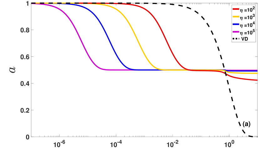
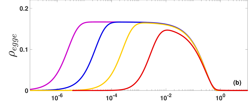
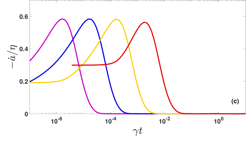
Figure 4: Numerical results showing super- and subradiance. (a) Upper-level population for different optical depths $\eta$; vacuum decay dynamics are shown for comparison (dashed black line). (b) Two-atom coherence $\rho_{egge}=\langle\sigma_{1}^{+}\sigma_{2}^{-}\rangle$. (c) Rate of loss of population (proportional to the radiated intensity per atom) normalized by optical depth $\eta$. Time is given in terms of vacuum life time $\gamma^{-1}$.

A simulation of the time-evolution is shown in Fig. 4, plotted with different optical depth $\eta$. Note that the chosen optical depths cover several orders of magnitude, ranging from the typical value for a cold-atom experiment ($\sim\!\!10^{2}$)[66], to the value that can be reached by Rydberg-state superradiance ($\sim\!\!10^{5}$)[11]. Fig. 4(a) shows the time-evolution of the average upper-level population $a$. As a comparison, the vacuum spontaneous decay for independent atoms (VD) is plotted with the black dashed line. Note that the time axis is in logarithmic scale and in units of $1/\gamma$. We observe an early decay where the excited population rapidly drops from $1$ to $\sim\!1/2$ compared to the vacuum decay. This rapid decay corresponds to the superradiant outburst, as shown by the peaks in the radiated intensity plotted in Fig. 4(c). Note that the radiated intensity scales linearly with the optical depth as $\eta\propto N$, so that the total intensity scales as ${\cal O}(N^{2})$. Also, the times at which the maximum intensity occurs have an $N^{-1}$ dependence. After this initial superradiant phase, the radiation is suppressed at $a\approx 1/2$ and the system enters a subradiant regime. Fig. 4(b) shows the coherence from the two-atom density matrix. Its non-zero value that covers both the short-lived outburst and the long-lived suppressed emission verifies the cooperative nature of both phenomena. Starting from $\gamma t\approx 1$ where the coherence vanishes, the decay is enhanced again but attains only a relatively small value. This last phase of the time-evolution corresponds to radiation trapping [53, 67].

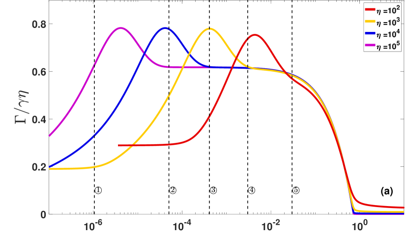
Figure 5: (a) Instantaneous cooperative decay rate $\Gamma$ normalized by optical depth $\eta$. (b) Line width of the radiated spectrum, normalized by optical depth. (c) The spectrum of $\Gamma$ at different times for $\eta=1000$. Numbered lines are plotted for times indicated in (a) and (b). Note that for all the plots $\Gamma$ is in units of $\gamma$.

Fig. 5(a) shows the time dependence of the approximated single-atom cooperative decay rate $\Gamma(\omega\!=\!0,t)$, by which the cooperative dynamic is mostly determined. Plotted are the dimensionless values normalized by the vacuum decay rate $\gamma$. $\Gamma$ builds up to its maximum during the superradiance phase, remains nearly constant during the subradiance phase and finally vanishes at the radiation trapping regime. Since in Fig. 5(a) the $\Gamma$’s are normalized by the optical depth $\eta$, we see that the actual $\Gamma$’s are indeed two to five orders of magnitude greater than the vacuum decay rate. Therefore, $\Gamma$ has the major contribution to the overall radiated intensity, and also possesses the ${\cal O}(N)$ dependence.

In Eq. (15) and Eq. (16a), $\Gamma(\omega,t)$ is expressed as the Fourier transform of the two-time field correlation with respect to the correlating time $\tau$, which, by virtue of the optical Wiener-Khinchin theorem [64], is related to the power spectral density of the field. The theorem is applicable to stationary processes, which is a well justified approximation as long as the correlating time scale $|\Delta\tau|$ is significantly shorter than the system evolution time scale $|\Delta t|$. Therefore, $\Gamma(\omega,t)$ is identical to the instantaneous spectrum of the cooperative radiation at time $t$. Fig. 5(c) shows the instantaneous spectra at different times for a sample with optical depth $\eta=10^{3}$, whereas Fig. 5(b) depicts the instantaneous linewidths, defined as the full width at half maximum. The circled numbers in Fig. 5(c) corresponds to the vertical dashed lines in Fig. 5(a,b). Note that the linewidths are broadened as the system evolves into the superradiant phase, and remain constant during the rest of the cooperative decay. The maximum linewidths scale with the optical depth $\eta$.

III.2 Subradiance

As can be seen qualitatively in the time evolution of the decay [e.g. Fig. 4(a)], the dynamics of the system turns very slow once the quick superradiant flash disappears. As we explain in this section, this phenomenon can be interpreted as a subradiant behavior. First, however, it is important to note that subradiance in fact emerges naturally in such a superradiant system. In Appendix  C, we demonstrate that the full Hilbert space consists of both the symmetric manifold and non-symmetric manifolds. Each manifold ladder decays and ends up in the ground state of the corresponding manifold, where the excitation “waits” for dipole-dipole interactions to take the system into the symmetric manifold such that the decay process can continue. In this subsection, we quantitatively investigate the subradiant phase of the homogeneous-gas model. For that, we introduce the quantity $\xi\equiv-\dot{a}/a$, which represents the number of emitted photons per excited atom per unit time. For a constant $\xi(t)=\gamma_{0}$, the dynamic of the system reduces to an exponential decay $a=a_{0}\,\rm{exp}(-\gamma_{0}t)$, where $\gamma_{0}$ is the inverse of the atomic lifetime $\tau_{0}$. A monotonically increasing (decreasing) $\xi(t)$ indicates a decay that is asymptotically faster (slower) than an exponential decay, a situation that can occur in the transition between exponential decays with different instantaneous decay rates. To see this, we expand $\xi(t)$ to the first order around $t$, i.e. $\xi(t)=\xi_{0}+\xi_{1}t$, and integrate to obtain

$$a = a_{0}e^{-\int\xi(t)dt}=a_{0}e^{-\xi_{1}t^{2}/2}e^{-\xi_{0}t}$$ (45)

$$\equiv a_{0}\,g(t)\,e^{-\xi_{0}t}$$

For small $\xi_{1}$, the dynamic can be seen as a modified exponential decay with an amplitude $g(t)$. With $\xi_{1}>0$, $g(t)$ is monotonically decreasing, which effectively describes a speedup of the decay.

Figure 6: Study of the time-dependent nature of subradiance through the quantity $-a/(\eta\dot{a})\equiv 1/\xi\eta$, plotted for different optical depths $\eta$. The constant plateau indicates an exponential decay, whereas the initial linear increase corresponds to a polynomial behavior. See main text for more explanation.

Figure 6 shows the inverse of $\xi\eta$ as a function of time. One can clearly see that $\xi$ remains constant during most of the subradiant phase. This is a signature of an exponential behavior featuring an extremely small instantaneous decay rate $\xi_{0}\sim\gamma/0.7\eta$, orders of magnitude smaller than the vacuum decay rate $\gamma$. Optically dense media therefore exhibit a strong subradiant effect, with a characteristic lifetime $\tau_{{\rm sub}}\!\sim\!1/\xi_{0}\!\sim\!\eta/\gamma$ that scales linearly with the optical depth. These two features —namely, the exponential behavior of subradiance and the scaling of its lifetime with the optical depth— agree with recent experimental observations in clouds of cold atoms [66]. Note also that the constant profile of $\xi$ finally disappears once the cooperative effect vanishes and radiation trapping starts to dominate.

III.3 Phase Change in Radiation Field

From Eq.(16a), $\Gamma(\omega,t)$ is expressed as the Fourier transform of the correlation function, up to a constant factor

$$\Gamma(\omega,t)\propto{\rm FT}\{\langle E^{-}(t)E^{+}(t+\Delta t)\rangle\}$$ (46)

That is, the two-time correlation of the field operators can be simply obtained by its inverse Fourier transform

$$\langle E^{-}(t)E^{+}(t+\Delta t)\rangle\propto\int_{-\infty}^{\infty}e^{-i\omega\Delta t}\Gamma(t,\omega)d\omega$$ (47)

The phase difference between the radiated field at different time is then related to its complex phase angle

$$\phi\equiv-\rm{arg}(\langle E^{-}(t)E^{+}(t+\Delta t)\rangle)$$ (48)

This argument follows from the correspondence between classical and quantum correlation function, where the field operators are related to the positive and negative components of the classical field as $\hat{E}^{\pm}\sim{\cal E}^{\pm}$. In the rotating frame and assuming a generic temporal relation of the classical field

$${\cal E}(t+\Delta t)\propto e^{-i\phi}{\cal E}(t)$$ (49)

The quantum correlation function can then be interpreted as

$$\langle\hat{E}^{-}(t)\hat{E}^{+}(t+\Delta t)\rangle\sim\overline{|{\cal E}|^{2}e^{-i\phi}}$$ (50)

where the over-line on right hand side denotes the ensemble average. Eq. (48) is therefore verified.

Figure 7: Phase angle of the field correlation function $\phi\equiv-\rm{arg}(\langle E^{+}(t)E^{-}(t+\Delta t)\rangle)$. We choose an adaptive time step $\Delta t=\alpha t$, with different constants $\alpha$. A phase change appears during the decay process. Its maximum, indicated by the dashed line, is reached during the superradiant burst, as shown by the excited state population profile in the inset.

Fig. 7 shows the normalized phase angle with adaptive time intervals $\Delta t=\alpha t$, for various constant values of $\alpha$ and an optical depth $\eta=1000$. With $\phi\!>\!0$, the radiated field exhibits an advancing phase change. This result is qualitatively in agreement with Ref. [11], where a phase turn was discovered in Rydberg-Rydberg superradiance transitions.

IV Conclusions

We have introduced an integrated method to describe an extended and optically dense ensemble of $N$ two-level atoms that radiate collectively. The dynamics of the system is formally derived with the help of the Keldysh formalism. By tracing out the quantized field and $(N-2)$ atoms, a two-atom effective description is obtained. The two-atom representation vastly reduces the difficulty of the many-body problem, while still capturing the essential collective nature of the full system. We established a self-consistent formalism that is satisfied at each physical time, and is thus able to solve the full time-evolution of the two-atom system. For a homogeneous gas of inverted two-level atoms, we demonstrate that the cooperative phenomena – both superradiance and subradiance – successively occur during the decay. These phenomena are characterized by a non-zero coherence $\rho_{eg,ge}$. The early-time superradiance features an outburst of radiated intensity that is proportional to the optical depth of the sample, while the cooperative decay rate is found to be orders of magnitude greater than the spontaneous decay rate of independent atoms. The subradiant phase, on the other hand, exhibits a slow exponential decay, having a decay rate that is inversely proportional to the optical depth, and a lifetime that scales linearly with the optical depth. Additionally, we find a broadened linewidth and a phase change of the radiated field during the cooperative decay, which qualitatively match with recent experimental observations of superradiant decay [11]. At late times, when the coherence vanishes, the system enters a radiation trapping regime. These results therefore present our formalism as a powerful method to study cooperative effects in radiative many-body systems.

The formalism presented in this letter can also be leveraged to study optically dense systems in the presence of an external classical driving field and may elucidate the nature of the resulting steady states, which are of great interest due to their potential to exhibit bistability and spin-squeezing effects [68, 21]. Additionally, this method can be readily employed to investigate the cooperative decay of systems with other geometries such as three-dimensional and two-dimensional ordered arrays of atoms [69]. Alternatively, lifting some symmetry constraints considered in this work could allow to study finite size effects of large samples.

Appendix A Keldysh Formalism[56]

Figure 8: Schwinger-Keldysh contour in the time-evolution operator $S_{\cal C}$. The time integral starts from $-\infty$ on the upper branch, turns at present time $t$, and then goes back to $-\infty$ on the lower branch. Note that the time-ordering operator ${\cal T}_{\cal C}$ is defined differently on each branch.

Suppose we have a Hamiltonian separated into free and interaction terms.

$$H\;=\;H_{0}+V$$

Recall the time-evolution operators in the Schrodinger and the interaction pictures. Each of them is assigned with a proper time-ordering operator.

$$U(t,t_{0}) ={\cal T}e^{-\frac{i}{\hbar}\int_{t_{0}}^{t}d\tau H(\tau)}$$ (51a)

$$U_{0}(t,t_{0}) ={\cal T}e^{-\frac{i}{\hbar}\int_{t_{0}}^{t}d\tau H_{0}(\tau)}$$ (51b)

$$U_{I}(t,t_{0}) =U_{0}^{\dagger}(t,t_{0})U(t,t_{0})={\cal T}e^{-\frac{i}{\hbar}\int_{t_{0}}^{t}d\tau V^{I}(\tau)}$$ (51c)

where $V^{I}(t)=U_{0}^{\dagger}(t,t_{0})V(t)U_{0}(t,t_{0})$ is the interaction term in the interaction picture. We consider $t>t_{0}$ in all cases. The key of Keldysh formalism is that the expectation value of any operator can alternatively be written in terms of those time-evolution operators

$$\langle\hat{O}\rangle(t) = {\rm Tr}\left(\rho(t)\hat{O}\right)$$ (52)

$$= {\rm Tr}\left(U(t,t_{0})\rho_{0}U^{\dagger}(t,t_{0})\hat{O}\right)$$

$$= {\rm Tr}\left(U(t,t_{0})\rho_{0}U^{\dagger}(t,t_{0})U_{0}(t,t_{0})\hat{O}^{I}(t)U_{0}^{\dagger}(t,t_{0})\right)$$

$$= {\rm Tr}\left(\rho_{0}U^{\dagger}(t,t_{0})U_{0}(t,t_{0})\hat{O}^{I}(t)U_{0}^{\dagger}(t,t_{0})U(t,t_{0})\right)$$

$$= {\rm Tr}\left(\rho_{0}U_{I}^{\dagger}(t,t_{0})\hat{O}^{I}(t)U_{I}(t,t_{0})\right)$$

The second step makes use of the time evolution of the density matrix in Schrodinger’s picture. The third step expresses $\hat{O}$ in terms of the interaction picture operator $\hat{O}^{I}(t)$. While in the last step, we make use of the definition of $U_{I}(t,t_{0})$. By defining the time-evolution operator along the Keldysh contour (see Fig. 8)

$$S_{\cal C}\;\equiv\;{\cal T}_{\cal C}e^{-\frac{i}{\hbar}\int\limits_{\cal C}d\check{\tau}\,V^{I}(\check{\tau})}$$ (53)

the expectation value of $\hat{O}$ can be written as

$$\langle\hat{O}\rangle(t)={\rm Tr}\left(\rho_{0}{\cal T}_{\cal C}{\cal S}_{\cal C}\hat{O}^{I}(t)\right)\equiv\left\langle{\cal T}_{\cal C}{\cal S}_{\cal C}\hat{O}^{I}(t)\right\rangle_{0}$$ (54)

Note that the ${\cal S}_{\cal C}$ in this expression includes the two-fold $U_{I}^{\dagger}(t,t_{0})$ and $U_{I}(t,t_{0})$ in Eq. (52). Now that the matrix elements of our density operator are exactly the expectation value of the corresponding projection operators [70], i.e. $\rho_{\alpha\beta}=\left\langle\left|\beta\right\rangle\left\langle\alpha\right|\right\rangle$, it is possible to write the density matrix elements in terms of ${\cal S}_{\cal C}$ and projection operators in the interaction picture.

$$\rho_{\alpha\beta}(t)={\rm Tr}\left(\rho_{0}{\cal T}_{\cal C}{\cal S}_{\cal C}P_{\beta\alpha}^{I}(t)\right)\equiv\left\langle{\cal T}_{\cal C}{\cal S}_{\cal C}P_{\beta\alpha}^{I}(t)\right\rangle_{0}$$ (55)

Appendix B Cumulant Expansion for Effective Time-evolution Operator

Suppose $X$, $Y$ and $Z$ are classical stochastic variables. The cumulant averages are defined as[71]

$$\left\langle\!\left\langle X\right\rangle\!\right\rangle \equiv \left\langle X\right\rangle$$

$$\left\langle\!\left\langle XY\right\rangle\!\right\rangle \equiv \left\langle XY\right\rangle-\left\langle X\right\rangle\left\langle Y\right\rangle$$

$$\left\langle\!\left\langle XYZ\right\rangle\!\right\rangle \equiv \left\langle XYZ\right\rangle-\left\langle X\right\rangle\left\langle YZ\right\rangle-\left\langle Y\right\rangle\left\langle XZ\right\rangle-\left\langle Z\right\rangle\left\langle XY\right\rangle$$

$$+2\left\langle X\right\rangle\left\langle Y\right\rangle\left\langle Z\right\rangle$$

$$...$$

Comparing term by term, we readily obtain

$$\left\langle e^{X}\right\rangle=\left\langle{\rm exp}\left\{{\sum_{n=0}^{\infty}}\frac{1}{n!}X^{n}\right\}\right\rangle={\rm exp}\left\{{\sum_{n=1}^{\infty}}\frac{1}{n!}\left\langle\!\left\langle X^{n}\right\rangle\!\right\rangle\right\}$$ (56)

This formula also works for operators, with the constrain that they mutually commute. This condition is satisfied with a time-ordering operator ${\cal T}_{\cal C}$ assigned to each term. Therefore, we can derive Eq. (5) from Eq. (4).

Appendix C Subradiant states

In Fig. 4(a), the time-evolution of the initially inverted homogeneous gas exhibits a transition from the superradiant phase to the subradiant phase. This transition can be understood by means of the full manifolds of the Hilbert space, which includes both the symmetric Dicke states and the non-symmetric states. In Fig. 9, we demonstrate this process with the simple example of a three-particle system, as well as with a generic $N-$particle system.

Because of the broken permutational symmetry of finite-size systems, dipole-dipole interactions (illustrated by the green arrows) mediate transitions between the symmetric Dicke states and the non-symmetric states. Once the system evolves into one of the non-symmetric states, it cascades down the “ladder” through spontaneous superradiant decay (yellow arrows) until it reaches the subradiant states. There, the excitation remains trapped until the dipole-dipole interactions cause new transitions to other states that can radiate. This qualitatively explains the long lifetime of the subradiant plateau at $a\!\sim\!1/2$.

The non-symmetric states can be obtained from the symmetric Dicke states and the bare eigenstates of the free Hamiltonian by using the Gram-Schmidt orthogonalization method. Repeatedly applying the collective lowering operator $\sum_{i}\sigma_{i}$, one can keep track of the route of the decay path and finally reach the subradiant states.

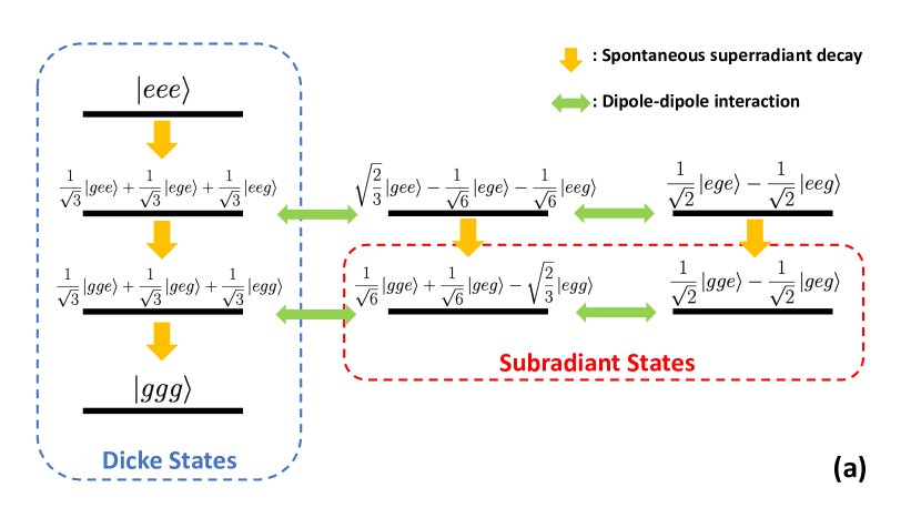
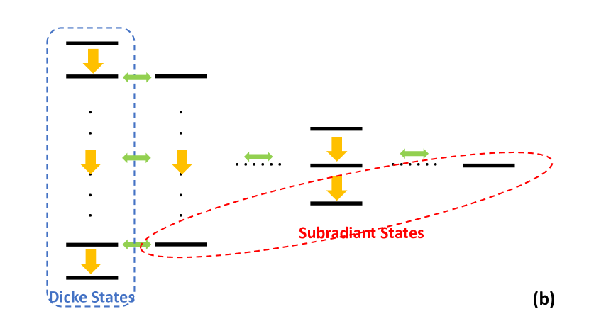
Figure 9: Schematic diagram of the cooperative radiation process for (a) three-particle system and (b) N-particle system.

Appendix D Derivation of Master Equation

We start with the effective time-evolution operator for the two atom system given in Eq. (14)

$$\dot{\cal S}^{\rm eff}_{\cal C} = {\cal T}_{\cal C}\frac{d}{dt}\bigg{(}-\frac{i}{\hbar}\int_{\cal C}d\tau_{1}\left\langle V^{I}(\tau_{1})\right\rangle$$

$$-\frac{1}{2\hbar^{2}}\iint_{\cal C}d\tau_{1}d\tau_{2}\left\langle\!\left\langle{\cal T}_{\cal C}V^{I}(\tau_{1})V^{I}(\tau_{2})\right\rangle\!\right\rangle\bigg{)}e^{P}$$

The first term can be expanded as

$$\frac{d}{dt}\left(-\frac{i}{\hbar}\int_{\cal C}d\tau_{1}\left\langle V^{I}(\tau_{1})\right\rangle\right)$$

$$= -\frac{i}{\hbar}\frac{d}{dt}\int_{\cal C}d\check{\tau}\left\langle V^{I}(\check{\tau})\right\rangle$$

$$= \frac{i}{\hbar}\frac{d}{dt}\int_{\cal C}d\check{\tau}\sum_{i,\mu}\left(p^{+}_{i\mu}(\check{\tau}){\cal E}^{-}_{L,i\mu}(\check{\tau})+p^{-}_{i\mu}(\check{\tau}){\cal E}^{+}_{L,i\mu}(\check{\tau})\right)$$

$$= \frac{i}{\hbar}\sum_{i,\mu}\wp_{\mu}\left\{\left(\sigma_{i\mu}(t^{+}){\cal E}^{-}_{L,i\mu}(t^{+})+\sigma_{i\mu}^{\dagger}(t^{+}){\cal E}^{+}_{L,i\mu}(t^{+})\right)\right.$$

$$\left.-\left(\sigma_{i\mu}(t^{-}){\cal E}^{-}_{L,i\mu}(t^{-})+\sigma_{i\mu}^{\dagger}(t^{-}){\cal E}^{+}_{L,i\mu}(t^{-})\right)\right\}$$

Therefore, the first and second order terms of $\left\langle{\cal T}_{\cal C}\dot{\cal S}^{\rm eff}_{\cal C}P^{I}_{\beta\alpha}(t)\right\rangle$ are

$$FOT=\left\langle{\cal T}_{\cal C}\frac{d}{dt}\left(-\frac{i}{\hbar}\int_{\cal C}d\tau_{1}\left\langle V^{I}(\tau_{1})\right\rangle\right)P^{I}_{\beta\alpha}(t)e^{P}\right\rangle$$

$$= \frac{i}{\hbar}\sum_{i,\mu}\wp_{\mu}\left\langle{\cal T}_{\cal C}\left\{\sigma_{i\mu}(t^{+}){\cal E}^{-}_{L,i\mu}(t^{+})+\sigma_{i\mu}^{\dagger}(t^{+}){\cal E}^{+}_{L,i\mu}(t^{+})-\sigma_{i\mu}(t^{-}){\cal E}^{-}_{L,i\mu}(t^{-})-\sigma_{i\mu}^{\dagger}(t^{-}){\cal E}^{+}_{L,i\mu}(t^{-})\right\}P^{I}_{\beta\alpha}(t){\cal S}^{\rm eff}_{\cal C}\right\rangle$$

$$= \frac{i}{\hbar}\sum_{i,\mu}\wp_{\mu}{\rm Tr}\left\{\rho(t)\left\{P_{\beta\alpha}\sigma_{i\mu}{\cal E}^{-}_{L,i\mu}+P_{\beta\alpha}\sigma_{i\mu}^{\dagger}{\cal E}^{+}_{L,i\mu}-\sigma_{i\mu}{\cal E}^{-}_{L,i\mu}P_{\beta\alpha}-\sigma_{i\mu}^{\dagger}{\cal E}^{+}_{L,i\mu}P_{\beta\alpha}\right\}\right\}$$

$$= \frac{i}{\hbar}\sum_{i,\mu}\wp_{\mu}{\rm Tr}\left\{P_{\beta\alpha}\sigma_{i\mu}{\cal E}^{-}_{L,i\mu}\rho(t)+P_{\beta\alpha}\sigma_{i\mu}^{\dagger}{\cal E}^{+}_{L,i\mu}\rho(t)-\rho(t)\sigma_{i\mu}{\cal E}^{-}_{L,i\mu}P_{\beta\alpha}-\rho(t)\sigma_{i\mu}^{\dagger}{\cal E}^{+}_{L,i\mu}P_{\beta\alpha}\right\}$$

$$= \frac{i}{\hbar}\sum_{i,\mu}\wp_{\mu}\left\langle\alpha\right|\left\{\sigma_{i\mu}{\cal E}^{-}_{L,i\mu}\rho(t)+\sigma_{i\mu}^{\dagger}{\cal E}^{+}_{L,i\mu}\rho(t)-\rho(t)\sigma_{i\mu}{\cal E}^{-}_{L,i\mu}-\rho(t)\sigma_{i\mu}^{\dagger}{\cal E}^{+}_{L,i\mu}\right\}\left|\beta\right\rangle$$

$$= \frac{i}{\hbar}\sum_{i,\mu}\wp_{\mu}\left\langle\alpha\right|\left[\sigma_{i\mu}{\cal E}^{-}_{L,i\mu}+\sigma_{i\mu}^{\dagger}{\cal E}^{+}_{L,i\mu},\rho(t)\right]\left|\beta\right\rangle$$

$$SOT = \left\langle{\cal T}_{\cal C}ST{\cal S}^{\rm eff}_{\cal C}P^{I}_{\beta\alpha}(t)\right\rangle$$

$$= \bigg{\langle}-{\cal T}_{\cal C}\sum_{i\mu,j\nu}\frac{\wp_{\mu}\wp_{\nu}}{2\hbar^{2}}\bigg{(}$$

$$\int_{-\infty}^{t}d\tau_{2}^{+}\left\{\sigma_{i\mu}(t^{+})D_{i\mu,j\nu}^{++}(t^{+},\tau_{2}^{+})\sigma_{j\nu}^{\dagger}(\tau_{2}^{+})e^{-i\delta\omega(t^{+}-\tau_{2}^{+})}+\sigma_{i\mu}^{\dagger}(t^{+})C_{i\mu,j\nu}^{++}(t^{+},\tau_{2}^{+})\sigma_{j\nu}(\tau_{2}^{+})e^{i\delta\omega(t^{+}-\tau_{2}^{+})}\right\}$$

$$+ \int_{-\infty}^{t}d\tau_{1}^{+}\left\{\sigma_{i\mu}(\tau_{1}^{+})D_{i\mu,j\nu}^{++}(\tau_{1}^{+},t^{+})\sigma_{j\nu}^{\dagger}(t^{+})e^{-i\delta\omega(\tau_{1}^{+}-t^{+})}+\sigma_{i\mu}^{\dagger}(\tau_{1}^{+})C_{i\mu,j\nu}^{++}(\tau_{1}^{+},t^{+})\sigma_{j\nu}(t^{+})e^{i\delta\omega(\tau_{1}^{+}-t^{+})}\right\}$$

$$+ \int_{-\infty}^{t}d\tau_{2}^{-}\left\{\sigma_{i\mu}(t^{-})D_{i\mu,j\nu}^{--}(t^{-},\tau_{2}^{-})\sigma_{j\nu}^{\dagger}(\tau_{2}^{-})e^{-i\delta\omega(t^{-}-\tau_{2}^{-})}+\sigma_{i\mu}^{\dagger}(t^{-})C_{i\mu,j\nu}^{--}(t^{-},\tau_{2}^{-})\sigma_{j\nu}(\tau_{2}^{-})e^{i\delta\omega(t^{-}-\tau_{2}^{-})}\right\}$$

$$+ \int_{-\infty}^{t}d\tau_{1}^{-}\left\{\sigma_{i\mu}(\tau_{1}^{-})D_{i\mu,j\nu}^{--}(\tau_{1}^{-},t^{-})\sigma_{j\nu}^{\dagger}(t^{-})e^{-i\delta\omega(\tau_{1}^{-}-t^{-})}+\sigma_{i\mu}^{\dagger}(\tau_{1}^{-})C_{i\mu,j\nu}^{--}(\tau_{1}^{-},t^{-})\sigma_{j\nu}(t^{-})e^{i\delta\omega(\tau_{1}^{-}-t^{-})}\right\}$$

$$- \int_{-\infty}^{t}d\tau_{2}^{-}\left\{\sigma_{i\mu}(t^{+})D_{i\mu,j\nu}^{+-}(t^{+},\tau_{2}^{-})\sigma_{j\nu}^{\dagger}(\tau_{2}^{-})e^{-i\delta\omega(t^{+}-\tau_{2}^{-})}+\sigma_{i\mu}^{\dagger}(t^{+})C_{i\mu,j\nu}^{+-}(t^{+},\tau_{2}^{-})\sigma_{j\nu}(\tau_{2}^{-})e^{i\delta\omega(t^{+}-\tau_{2}^{-})}\right\}$$

$$- \int_{-\infty}^{t}d\tau_{1}^{+}\left\{\sigma_{i\mu}(\tau_{1}^{+})D_{i\mu,j\nu}^{+-}(\tau_{1}^{+},t^{-})\sigma_{j\nu}^{\dagger}(t^{-})e^{-i\delta\omega(\tau_{1}^{+}-t^{-})}+\sigma_{i\mu}^{\dagger}(\tau_{1}^{+})C_{i\mu,j\nu}^{+-}(\tau_{1}^{+},t^{-})\sigma_{j\nu}(t^{-})e^{i\delta\omega(\tau_{1}^{+}-t^{-})}\right\}$$

$$- \int_{-\infty}^{t}d\tau_{2}^{+}\left\{\sigma_{i\mu}(t^{-})D_{i\mu,j\nu}^{-+}(t^{-},\tau_{2}^{+})\sigma_{j\nu}^{\dagger}(\tau_{2}^{+})e^{-i\delta\omega(t^{-}-\tau_{2}^{+})}+\sigma_{i\mu}^{\dagger}(t^{-})C_{i\mu,j\nu}^{-+}(t^{-},\tau_{2}^{+})\sigma_{j\nu}(\tau_{2}^{+})e^{i\delta\omega(t^{-}-\tau_{2}^{+})}\right\}$$

$$- \int_{-\infty}^{t}d\tau_{1}^{-}\left\{\sigma_{i\mu}(\tau_{1}^{-})D_{i\mu,j\nu}^{-+}(\tau_{1}^{-},t^{+})\sigma_{j\nu}^{\dagger}(t^{+})e^{-i\delta\omega(\tau_{1}^{-}-t^{+})}+\sigma_{i\mu}^{\dagger}(\tau_{1}^{-})C_{i\mu,j\nu}^{-+}(\tau_{1}^{-},t^{+})\sigma_{j\nu}(t^{+})e^{i\delta\omega(\tau_{1}^{-}-t^{+})}\right\}\bigg{)}$$

$${\cal S}^{\rm eff}_{\cal C}P^{I}_{\beta\alpha}(t)\bigg{\rangle}$$

There are in total 8 terms in $SOT$, here we show the calculation for the first term.

$$T_{1} = \bigg{\langle}{\cal T}_{\cal C}\int_{-\infty}^{t}d\tau_{2}^{+}\left\{\sigma_{i\mu}(t^{+})D_{i\mu,j\nu}^{++}(t^{+},\tau_{2}^{+})\sigma_{j\nu}^{\dagger}(\tau_{2}^{+})e^{-i\delta\omega(t^{+}-\tau_{2}^{+})}\right.$$

$$\left.+\sigma_{i\mu}^{\dagger}(t^{+})C_{i\mu,j\nu}^{++}(t^{+},\tau_{2}^{+})\sigma_{j\nu}(\tau_{2}^{+})e^{i\delta\omega(t^{+}-\tau_{2}^{+})}\right\}{\cal S}^{\rm eff}_{\cal C}P^{I}_{\beta\alpha}(t)\bigg{\rangle}$$

$$= \bigg{\langle}{\cal T}_{\cal C}\int_{-\infty}^{t}d\tau_{2}^{+}\left\{P^{I}_{\beta\alpha}(t)\sigma_{i\mu}(t^{+})\sigma_{j\nu}^{\dagger}(\tau_{2}^{+})D_{i\mu,j\nu}^{++}(t^{+},\tau_{2}^{+})e^{-i\delta\omega(t^{+}-\tau_{2}^{+})}\right.$$

$$\left.+P^{I}_{\beta\alpha}(t)\sigma_{i\mu}^{\dagger}(t^{+})\sigma_{j\nu}(\tau_{2}^{+})C_{i\mu,j\nu}^{++}(t^{+},\tau_{2}^{+})e^{i\delta\omega(t^{+}-\tau_{2}^{+})}\right\}{\cal S}^{\rm eff}_{\cal C}\bigg{\rangle}$$

$$= \bigg{\langle}\int_{-\infty}^{t}d\tau_{2}^{+}\left\{P^{H}_{\beta\alpha}(t)\sigma_{i\mu}^{H}(t^{+})\sigma_{j\nu}^{\dagger H}(\tau_{2}^{+})D_{i\mu,j\nu}^{++}(t^{+},\tau_{2}^{+})e^{-i\delta\omega(t^{+}-\tau_{2}^{+})}\right.$$

$$\left.+P^{H}_{\beta\alpha}(t)\sigma_{i\mu}^{\dagger H}(t^{+})\sigma_{j\nu}^{H}(\tau_{2}^{+})C_{i\mu,j\nu}^{++}(t^{+},\tau_{2}^{+})e^{i\delta\omega(t^{+}-\tau_{2}^{+})}\right\}\bigg{\rangle}$$

$$= \bigg{\langle}\int_{-\infty}^{t}d\tau^{\prime}\left\{P^{H}_{\beta\alpha}(t)\sigma_{i\mu}^{H}(t)\sigma_{j\nu}^{\dagger H}(\tau^{\prime})D_{i\mu,j\nu}^{++}(t,\tau^{\prime})e^{-i\omega(t-\tau^{\prime})}\right.$$

$$\left.+P^{H}_{\beta\alpha}(t)\sigma_{i\mu}^{\dagger H}(t)\sigma_{j\nu}^{H}(\tau^{\prime})C_{i\mu,j\nu}^{++}(t,\tau^{\prime})e^{i\omega(t-\tau^{\prime})}\right\}\bigg{\rangle}$$

$$= \bigg{\langle}\int_{-\infty}^{t}d\tau^{\prime}\left\{P^{H}_{\beta\alpha}(t)\sigma_{i\mu}^{H}(t)\sigma_{j\nu}^{\dagger H}(\tau^{\prime})\left\langle\!\left\langle E^{-}_{i\mu}(t)E^{+}_{j\nu}(\tau^{\prime})\right\rangle\!\right\rangle e^{-i\omega(t-\tau^{\prime})}\right.$$

$$\left.+P^{H}_{\beta\alpha}(t)\sigma_{i\mu}^{\dagger H}(t)\sigma_{j\nu}^{H}(\tau^{\prime})\left\langle\!\left\langle E^{+}_{i\mu}(t)E^{-}_{j\nu}(\tau^{\prime})\right\rangle\!\right\rangle e^{i\omega(t-\tau^{\prime})}\right\}\bigg{\rangle}$$

$$= \bigg{\langle}\int^{+\infty}_{0}d\tau\left\{P^{H}_{\beta\alpha}(t)\sigma_{i\mu}^{H}(t)\sigma_{j\nu}^{\dagger H}(t-\tau)\left\langle\!\left\langle E^{-}_{i\mu}(t)E^{+}_{j\nu}(t-\tau)\right\rangle\!\right\rangle e^{-i\omega\tau}\right.$$

$$\left.+P^{H}_{\beta\alpha}(t)\sigma_{i\mu}^{\dagger H}(t)\sigma_{j\nu}^{H}(t-\tau)\left\langle\!\left\langle E^{+}_{i\mu}(t)E^{-}_{j\nu}(t-\tau)\right\rangle\!\right\rangle e^{i\omega\tau}\right\}\bigg{\rangle}$$

$$= \bigg{\langle}\int^{+\infty}_{0}d\tau\left\{P^{H}_{\beta\alpha}(t)\sigma_{i\mu}^{H}(t)\sigma_{j\nu}^{\dagger H}(t)\left\langle\!\left\langle E^{-}_{i\mu}(t)E^{+}_{j\nu}(t-\tau)\right\rangle\!\right\rangle e^{-i\omega\tau}\right.$$

$$\left.+P^{H}_{\beta\alpha}(t)\sigma_{i\mu}^{\dagger H}(t)\sigma_{j\nu}^{H}(t)\left\langle\!\left\langle E^{+}_{i\mu}(t+\tau)E^{-}_{j\nu}(t)\right\rangle\!\right\rangle e^{i\omega\tau}\right\}\bigg{\rangle}$$

$$= \left\langle\alpha\right|\int^{+\infty}_{0}d\tau\left\{\sigma_{i\mu}\sigma_{j\nu}^{\dagger}\rho(t)\left\langle\!\left\langle E^{-}_{i\mu}(t)E^{+}_{j\nu}(t-\tau)\right\rangle\!\right\rangle e^{-i\omega\tau}+\sigma_{j\nu}^{\dagger}\sigma_{i\mu}\rho(t)\left\langle\!\left\langle E^{+}_{j\nu}(t+\tau)E^{-}_{i\mu}(t)\right\rangle\!\right\rangle e^{i\omega\tau}\right\}\left|\beta\right\rangle$$

In the 1st and 2nd steps all operators are in interaction picture, in the 4th step we remove the superscript on $t$ and replace $\delta\omega$ by $\omega$, $\tau_{2}$ by $\tau^{\prime}$. In the 6th step we make a variable substitution $\tau=t-\tau^{\prime}$. In the 7th step we make the Markov approximation, such that all atomic operators depend on t. The term with $e^{i\omega\tau}$ has $\tau$ on the “wrong” side, $\left\langle\!\left\langle E^{\mp}_{i\mu}(t)E^{\pm}_{j\nu}(t-\tau)\right\rangle\!\right\rangle\approx\left\langle\!\left\langle E^{\mp}_{i\mu}(t+\tau)E^{\pm}_{j\nu}(t)\right\rangle\!\right\rangle$. In the last step we go back to Schrodinger’s picture and reassign dummy indexes if needed.

Here we list the results of the remaining seven terms:

$$T_{2} = \left\langle\alpha\right|\int^{+\infty}_{0}d\tau\left\{\sigma_{j\nu}^{\dagger}\sigma_{i\mu}\rho(t)\left\langle\!\left\langle E^{+}_{j\nu}(t+\tau)E^{-}_{i\mu}(t)\right\rangle\!\right\rangle e^{i\omega\tau}+\sigma_{i\mu}\sigma_{j\nu}^{\dagger}\rho(t)\left\langle\!\left\langle E^{-}_{i\mu}(t)E^{+}_{j\nu}(t-\tau)\right\rangle\!\right\rangle e^{-i\omega\tau}\right\}\left|\beta\right\rangle$$

$$T_{3} = \left\langle\alpha\right|\int^{+\infty}_{0}d\tau\left\{\rho(t)\sigma_{j\nu}^{\dagger}\sigma_{i\mu}\left\langle\!\left\langle E^{+}_{j\nu}(t-\tau)E^{-}_{i\mu}(t)\right\rangle\!\right\rangle e^{-i\omega\tau}+\rho(t)\sigma_{i\mu}\sigma_{j\nu}^{\dagger}\left\langle\!\left\langle E^{-}_{i\mu}(t)E^{+}_{j\nu}(t+\tau)\right\rangle\!\right\rangle e^{i\omega\tau}\right\}\left|\beta\right\rangle$$

$$T_{4} = \left\langle\alpha\right|\int^{+\infty}_{0}d\tau\left\{\rho(t)\sigma_{i\mu}\sigma_{j\nu}^{\dagger}\left\langle\!\left\langle E^{-}_{i\mu}(t)E^{+}_{j\nu}(t+\tau)\right\rangle\!\right\rangle e^{i\omega\tau}+\rho(t)\sigma_{j\nu}^{\dagger}\sigma_{i\mu}\left\langle\!\left\langle E^{+}_{j\nu}(t-\tau)E^{-}_{i\mu}(t)\right\rangle\!\right\rangle e^{-i\omega\tau}\right\}\left|\beta\right\rangle$$

$$T_{5} = \left\langle\alpha\right|\int^{+\infty}_{0}d\tau\left\{\sigma_{i\mu}\rho(t)\sigma_{j\nu}^{\dagger}\left\langle\!\left\langle E^{+}_{j\nu}(t-\tau)E^{-}_{i\mu}(t)\right\rangle\!\right\rangle e^{-i\omega\tau}+\sigma_{j\nu}^{\dagger}\rho(t)\sigma_{i\mu}\left\langle\!\left\langle E^{-}_{i\mu}(t)E^{+}_{j\nu}(t+\tau)\right\rangle\!\right\rangle e^{i\omega\tau}\right\}\left|\beta\right\rangle$$

$$T_{6} = \left\langle\alpha\right|\int^{+\infty}_{0}d\tau\left\{\sigma_{i\mu}\rho(t)\sigma_{j\nu}^{\dagger}\left\langle\!\left\langle E^{+}_{j\nu}(t+\tau)E^{-}_{i\mu}(t)\right\rangle\!\right\rangle e^{i\omega\tau}+\sigma_{j\nu}^{\dagger}\rho(t)\sigma_{i\mu}\left\langle\!\left\langle E^{-}_{i\mu}(t)E^{+}_{j\nu}(t-\tau)\right\rangle\!\right\rangle e^{-i\omega\tau}\right\}\left|\beta\right\rangle$$

$$T_{7} = \left\langle\alpha\right|\int^{+\infty}_{0}d\tau\left\{\sigma_{j\nu}^{\dagger}\rho(t)\sigma_{i\mu}\left\langle\!\left\langle E^{-}_{i\mu}(t)E^{+}_{j\nu}(t-\tau)\right\rangle\!\right\rangle e^{-i\omega\tau}+\sigma_{i\mu}\rho(t)\sigma_{j\nu}^{\dagger}\left\langle\!\left\langle E^{+}_{j\nu}(t+\tau)E^{-}_{i\mu}(t)\right\rangle\!\right\rangle e^{i\omega\tau}\right\}\left|\beta\right\rangle$$

$$T_{8} = \left\langle\alpha\right|\int^{+\infty}_{0}d\tau\left\{\sigma_{j\nu}^{\dagger}\rho(t)\sigma_{i\mu}\left\langle\!\left\langle E^{-}_{i\mu}(t)E^{+}_{j\nu}(t+\tau)\right\rangle\!\right\rangle e^{i\omega\tau}+\sigma_{i\mu}\rho(t)\sigma_{j\nu}^{\dagger}\left\langle\!\left\langle E^{+}_{j\nu}(t-\tau)E^{-}_{i\mu}(t)\right\rangle\!\right\rangle e^{-i\omega\tau}\right\}\left|\beta\right\rangle$$

with

$$SOT=-\sum_{i\mu,j\nu}\frac{\wp_{\mu}\wp_{\nu}}{2\hbar^{2}}\left(T_{1}+T_{2}+T_{3}+T_{4}-T_{5}-T_{6}-T_{7}-T_{8}\right)$$ (57)

Appendix E Retarded Green’s function in the medium

According to Ref. [60], the Fourier transform of the retarded Green’s function in the atomic medium can be written as

$$\mathbf{\tilde{\tilde{D}}^{ret}}(\vec{q},\omega_{0},t)=\left[\mathbf{1}+\mathbf{\tilde{\tilde{D}}_{0}^{ret}}(\vec{q},\omega_{0})\cdot\mathbf{\tilde{P}}^{ret}(\omega_{0},t)\right]^{-1}\cdot\mathbf{\tilde{\tilde{D}}_{0}^{ret}}(\vec{q},\omega_{0})$$ (58)

where $\mathbf{\tilde{P}}^{ret}(\omega_{0},t)$ is the polarization function and $\mathbf{\tilde{\tilde{D}}_{0}^{ret}}(\vec{q},\omega_{0})$ is the free-space retarded propagator.

The three-dimensional free-space retarded propagator in real space is

$$D_{0\alpha\beta}^{ret}(\vec{x},\omega_{0}) = -\frac{i\hbar}{4\pi\epsilon_{0}}\left(\frac{\omega_{0}^{2}}{c^{2}}\delta_{\alpha\beta}+\frac{\partial^{2}}{\partial x_{\alpha}\partial x_{\beta}}\right)\frac{e^{-i\omega_{0}r/c}}{r}$$ (59)

$$= -\frac{i\hbar k_{0}^{2}}{4\pi\epsilon_{0}}\left[\left(1-\frac{i}{k_{0}r}-\frac{1}{k_{0}^{2}r^{2}}\right)\delta_{\alpha\beta}+\left(-1+\frac{3i}{k_{0}r}+\frac{3}{k_{0}^{2}r^{2}}\right)\frac{x_{\alpha}x_{\beta}}{r^{2}}\right]\frac{e^{-ik_{0}r}}{r}$$

with $r=|\vec{x}|$ and $k_{0}=\omega_{0}/c$.

For a randomly polarized medium we can apply the polarization average $\langle\mathcal{P}_{\alpha}\mathcal{P}_{\beta}\rangle=\frac{1}{3}\delta_{\alpha\beta}$, which is equivalent to performing the orientation average

$$\frac{x_{\alpha}x_{\beta}}{r^{2}}\rightarrow\langle\frac{x_{\alpha}x_{\beta}}{r^{2}}\rangle=\frac{1}{3}\delta_{\alpha\beta}$$ (60)

Under these conditions, the free-space Green’s function becomes a spherical tensor

$$\mathbf{\tilde{D}}_{0}^{ret}(\vec{x},\omega_{0})=-\frac{i\hbar k_{0}^{2}}{6\pi\epsilon_{0}}\frac{e^{-ik_{0}r}}{r}\mathbf{1}$$ (61)

and the corresponding Fourier transform can be written as

$$\mathbf{\tilde{\tilde{D}}_{0}^{ret}}(\vec{q},\omega_{0}) = \int_{V_{\infty}}d^{3}\vec{x}\mathbf{\tilde{D}}_{0}^{ret}(\vec{x},\omega_{0})e^{i\vec{q}\vec{x}}e^{-\epsilon r}$$

$$= -\frac{2i\hbar k_{0}^{2}}{3\epsilon_{0}}\frac{1}{q^{2}-k_{0}^{2}+2ik_{0}\epsilon}\mathbf{1}$$

with $q=|\vec{q}|$ and where we have introduced the small, positive constant $\epsilon$ that allows convergence of the infinite volume integral.

The spherical nature of the Fourier transformed free-space propagator tensor turns Eq.(58) into a scalar equation. The retarded propagator in the atomic medium in momentum space takes now the simple form

$$\tilde{\tilde{D}}^{ret}(\vec{q},\omega_{0})=-\frac{2i\hbar k_{0}^{2}}{3\epsilon_{0}}\frac{1}{q^{2}-k_{0}^{2}\left(1+\frac{2i\hbar}{3\epsilon_{0}}\tilde{P}^{ret}\right)+2ik_{0}\epsilon}$$ (62)

Going back to real space, we obtain

$$\tilde{D}^{ret}(\vec{x},\omega_{0})=\frac{1}{(2\pi)^{3}}\int d^{3}\vec{q}\tilde{\tilde{D}}^{ret}(\vec{q},\omega_{0})e^{i\vec{q}\vec{x}}$$ (63)

$$= \frac{\hbar k_{0}^{2}}{6\pi^{2}\epsilon_{0}}\frac{1}{r}\int_{-\infty}^{\infty}dq\frac{qe^{-iqr}}{q^{2}-k_{0}^{2}\left(1+\frac{2i\hbar}{3\epsilon_{0}}\tilde{P}^{ret}-\frac{2i\epsilon}{k_{0}}\right)}$$ (64)

This integral is solved by contour integration along the real axis and a semicircle on the lower half plane, where $e^{-iqr}\rightarrow 0$ for large $|q|$. The integrand has two poles at $Re[q]\approx\pm k_{0}$. For an absorbing medium with $Re[\tilde{P}^{ret}]<0$, the pole at $Re[q]\approx k_{0}$ is in the lower half-plane, whereas the pole at $Re[q]\approx-k_{0}$ is in the lower one. The integral therefore results in a retarded propagator. Similarly, a retarded propagator is obtained for $Re[\tilde{P}^{ret}]=0$ by introducing a small, positive $\epsilon$. For an amplifying medium with $Re[\tilde{P}^{ret}]>0$, the pole at $Re[q]\approx k_{0}$ is in the upper half-plane. This problem arises from the fact that the retarded propagator of an amplifying medium increases exponentially with distance and can therefore not be Fourier transformed. Instead, a cutoff function should be included to take into account the finite size of the medium. Here, we will assume that the effect of the cutoff is analogous to adding a sufficiently large $\epsilon$ that moves the pole to the lower half-plane (see Ref. [60]).

Using the residue theorem, we finally find

$$\tilde{D}^{ret}(\vec{x},\omega_{0})=-\frac{i\hbar k_{0}^{2}}{6\pi\epsilon_{0}}\frac{e^{-iq_{0}r}}{r}$$ (65)

where

$$q_{0}=k_{0}\sqrt{1+\frac{2i\hbar}{3\epsilon_{0}}\tilde{P}^{ret}}$$ (66)

Appendix F Taylor Expansion in the Retarded Green’s Function

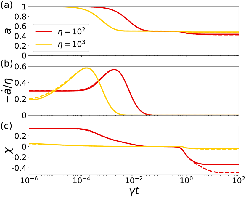
Figure 10: To show the validity of the Taylor expansion of $q_{0}=k_{0}\sqrt{1+i\chi}$, we compare the emission dynamics obtained with the exact expression (solid lines) and its Taylor-expanded form $q_{0}=k_{0}(1+i\chi/2)$ (dashed lines). (a) Upper-level population, (b) radiative intensity $\dot{a}/\eta$ and (c) expansion parameter $\chi$ in both scenarios and for $\eta=100$ ($C=\rho=10$) in red and $\eta=1000$ ($C=25$ and $\rho=40$) in yellow. The resulting dynamics are identical during the superradiant and subradiant phase, where $\chi$ remains small.

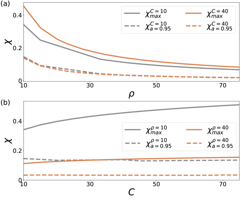
Figure 11: Expansion parameter $\chi$ (a) for fixed $C=10$ (silver) and $C=40$ (orange) as a function of $\rho$, as well as (b) for fixed $\rho=10$ (silver) and $\rho=40$ (orange) as a function of $C$. Solid line shows the maximum achieved value of $\chi$ during the superradiant phase, which occurs at $t=0$, or equivalently $a=1$. Dashed lines show $\chi$ when $a=0.95$, and demonstrate that $\chi$ remains small during most of the superradiant decay for all $C$ and $\rho$.

Let us focus on the non-driven case, for which

$$\tilde{P}^{ret}=\frac{\wp^{2}}{\hbar^{2}}\mathcal{N}\frac{2a-1}{\gamma/2+\Gamma-i\Delta}$$ (67)

Using the fact that $\gamma=\frac{\wp^{2}k_{0}^{3}}{3\pi\hbar\epsilon_{0}}$ and $C=\frac{\lambda_{0}^{3}\mathcal{N}}{(2\pi)^{2}}=2\pi\frac{\mathcal{N}}{k_{0}^{3}}$, Eq. (66) reduces to

$$q_{0}=k_{0}\sqrt{1+i\gamma C\frac{2a-1}{\gamma/2+\Gamma-i\Delta}}$$ (68)

One can define the quantity $\chi=\gamma C\frac{2a-1}{\gamma/2+\Gamma-i\Delta}$. For $|\chi|\ll 1$, $q_{0}$ can be Taylor expanded to first order

$$q_{0}=k_{0}\left(1+i\gamma\frac{C}{2}\frac{2a-1}{\gamma/2+\Gamma-i\Delta}\right)$$ (69)

and we retrieve the expression in Eq. (24) of the main text. The expansion parameter $\chi$ therefore sets the error of the Taylor expansion.

This approximation holds in the subradiant regime, where $a\approx 0.5$ and $\Gamma\propto\eta=C\rho$ (see Fig. 5), and $\chi$ therefore scales as $\chi\propto(2a-1)/\rho\rightarrow 0$ (region around $\gamma t=10^{-1}$ in Fig. 10c). For the superradiant outburst, we initially have $\Gamma(t\rightarrow 0)\approx\exp{(\eta/\Gamma)}$. This requires a sublinear dependence of $\Gamma$ on $\eta$. As a result, $\chi$ scales inversely proportional to $\rho$ at early times and additionally exhibits a strong sublinear increase as a function of $C$, as depicted in Fig. 11a and b, respectively. While the initial values can reach $\chi>0.5$ for certain combinations of $C$ and $\rho$, $\chi$ rapidly decreases during the superradiant outburst due to the fast increase of $\Gamma$ and the simultaneous decrease of $2a-1$. As shown in Fig. 11a-b, $\chi$ is always below $0.15$ when $a=0.95$ (dashed lines). Finally, $\chi$ becomes negative and grows again in absolute value during the radiation trapping regime ($a<0.5$). Although $\chi$ differs considerably for the exact and Taylor-expanded expressions ($\gamma t>10^{0}$ in Fig. 10c), $\dot{a}$ is smaller than $10^{-5}$ in this regime and no significant difference is observed in terms of excited population $a$ (Fig. 10a).

In conclusion, $\chi$ is sufficiently small during most of the evolution and no significant difference is observed between the exact solution (solid lines) and the Taylor-expanded one (dashed lines) in Fig. 10a-b, which confirms the validity of the approximation.

References

- Dicke [1954] R. H. Dicke, Coherence in spontaneous radiation processes, Phys. Rev. 93, 99 (1954).
- Gross and Haroche [1982] M. Gross and S. Haroche, Superradiance: An essay on the theory of collective spontaneous emission, Physics Reports 93, 301 (1982).
- Rehler and Eberly [1971] N. E. Rehler and J. H. Eberly, Superradiance, Phys. Rev. A 3, 1735 (1971).
- MacGillivray and Feld [1976] J. C. MacGillivray and M. S. Feld, Theory of superradiance in an extended, optically thick medium, Phys. Rev. A 14, 1169 (1976).
- Feher et al. [1958] G. Feher, J. P. Gordon, E. Buehler, E. A. Gere, and C. D. Thurmond, Spontaneous emission of radiation from an electron spin system, Phys. Rev. 109, 221 (1958).
- Skribanowitz et al. [1973] N. Skribanowitz, I. P. Herman, J. C. MacGillivray, and M. S. Feld, Observation of dicke superradiance in optically pumped hf gas, Phys. Rev. Lett. 30, 309 (1973).
- Szöke and Meiboom [1959] A. Szöke and S. Meiboom, Radiation damping in nuclear magnetic resonance, Phys. Rev. 113, 585 (1959).
- Inouye et al. [1999] S. Inouye, A. P. Chikkatur, D. M. Stamper-Kurn, J. Stenger, D. E. Pritchard, and W. Ketterle, Superradiant rayleigh scattering from a bose-einstein condensate, Science 285, 571 (1999).
- Baumann et al. [2010] K. Baumann, C. Guerlin, F. Brennecke, and T. Esslinger, Dicke quantum phase transition with a superfluid gas in an optical cavity, Nature 464, 1301 (2010).
- Wang et al. [2007] T. Wang, S. F. Yelin, R. Côté, E. E. Eyler, S. M. Farooqi, P. L. Gould, M. Koštrun, D. Tong, and D. Vrinceanu, Superradiance in ultracold rydberg gases, Phys. Rev. A 75, 033802 (2007).
- Grimes et al. [2017a] D. D. Grimes, S. L. Coy, T. J. Barnum, Y. Zhou, S. F. Yelin, and R. W. Field, Direct single-shot observation of millimeter-wave superradiance in rydberg-rydberg transitions, Phys. Rev. A 95, 043818 (2017a).
- Ferioli et al. [2021a] G. Ferioli, A. Glicenstein, L. Henriet, I. Ferrier-Barbut, and A. Browaeys, Storage and release of subradiant excitations in a dense atomic cloud, Phys. Rev. X 11, 021031 (2021a).
- Slama et al. [2007] S. Slama, S. Bux, G. Krenz, C. Zimmermann, and P. W. Courteille, Superradiant rayleigh scattering and collective atomic recoil lasing in a ring cavity, Phys. Rev. Lett. 98, 053603 (2007).
- Raimond et al. [1982] J. M. Raimond, P. Goy, M. Gross, C. Fabre, and S. Haroche, Collective absorption of blackbody radiation by rydberg atoms in a cavity: An experiment on bose statistics and brownian motion, Phys. Rev. Lett. 49, 117 (1982).
- Kaluzny et al. [1983] Y. Kaluzny, P. Goy, M. Gross, J. M. Raimond, and S. Haroche, Observation of self-induced rabi oscillations in two-level atoms excited inside a resonant cavity: The ringing regime of superradiance, Phys. Rev. Lett. 51, 1175 (1983).
- Haider et al. [2021] G. Haider, K. Sampathkumar, T. Verhagen, L. Nádvorník, F. J. Sonia, V. Valeš, J. Sýkora, P. Kapusta, P. Němec, M. Hof, O. Frank, Y.-F. Chen, J. Vejpravová, and M. Kalbáč, Superradiant emission from coherent excitons in van der waals heterostructures, Advanced Functional Materials 31, 2102196 (2021).
- Scheibner et al. [2007] M. Scheibner, T. Schmidt, L. Worschech, A. Forchel, G. Bacher, T. Passow, and D. Hommel, Superradiance of quantum dots, Nature Physics 3, 106 (2007).
- Rainò et al. [2018] G. Rainò, M. A. Becker, M. I. Bodnarchuk, R. F. Mahrt, M. V. Kovalenko, and T. Stöferle, Superfluorescence from lead halide perovskite quantum dot superlattices, Nature 563, 671 (2018).
- Meiser et al. [2009] D. Meiser, J. Ye, D. R. Carlson, and M. J. Holland, Prospects for a millihertz-linewidth laser, Phys. Rev. Lett. 102, 163601 (2009).
- Bohnet et al. [2012] J. G. Bohnet, Z. Chen, J. M. Weiner, D. Meiser, M. J. Holland, and J. K. Thompson, A steady-state superradiant laser with less than one intracavity photon, Nature 484, 78 (2012).
- Wolfe and Yelin [2014] E. Wolfe and S. F. Yelin, Spin squeezing by means of driven superradiance (2014), arXiv:1405.5288 [quant-ph] .
- Ma et al. [2011] J. Ma, X. Wang, C. Sun, and F. Nori, Quantum spin squeezing, Physics Reports 509, 89 (2011).
- González-Tudela and Porras [2013] A. González-Tudela and D. Porras, Mesoscopic entanglement induced by spontaneous emission in solid-state quantum optics, Phys. Rev. Lett. 110, 080502 (2013).
- Aparicio Alcalde et al. [2010] M. Aparicio Alcalde, A. H. Cardenas, N. F. Svaiter, and V. B. Bezerra, Entangled states and superradiant phase transitions, Phys. Rev. A 81, 032335 (2010).
- Lambert et al. [2004] N. Lambert, C. Emary, and T. Brandes, Entanglement and the phase transition in single-mode superradiance, Phys. Rev. Lett. 92, 073602 (2004).
- Ostermann et al. [2013] L. Ostermann, H. Ritsch, and C. Genes, Protected state enhanced quantum metrology with interacting two-level ensembles, Phys. Rev. Lett. 111, 123601 (2013).
- Facchinetti and Ruostekoski [2018] G. Facchinetti and J. Ruostekoski, Interaction of light with planar lattices of atoms: Reflection, transmission, and cooperative magnetometry, Phys. Rev. A 97, 023833 (2018).
- Henriet et al. [2019] L. Henriet, J. S. Douglas, D. E. Chang, and A. Albrecht, Critical open-system dynamics in a one-dimensional optical-lattice clock, Phys. Rev. A 99, 023802 (2019).
- Rubies-Bigorda et al. [2022] O. Rubies-Bigorda, V. Walther, T. L. Patti, and S. F. Yelin, Photon control and coherent interactions via lattice dark states in atomic arrays, Phys. Rev. Research 4, 013110 (2022).
- Ballantine and Ruostekoski [2021] K. E. Ballantine and J. Ruostekoski, Quantum single-photon control, storage, and entanglement generation with planar atomic arrays, PRX Quantum 2, 040362 (2021).
- Wang and Hioe [1973] Y. K. Wang and F. T. Hioe, Phase transition in the dicke model of superradiance, Phys. Rev. A 7, 831 (1973).
- Akkermans et al. [2008] E. Akkermans, A. Gero, and R. Kaiser, Photon localization and dicke superradiance in atomic gases, Phys. Rev. Lett. 101, 103602 (2008).
- Kirton and Keeling [2017] P. Kirton and J. Keeling, Suppressing and restoring the dicke superradiance transition by dephasing and decay, Phys. Rev. Lett. 118, 123602 (2017).
- Lehmberg [1970a] R. H. Lehmberg, Radiation from an -atom system. I. General formalism, Phys. Rev. A 2, 883 (1970a).
- Lehmberg [1970b] R. H. Lehmberg, Radiation from an -atom system. II. Spontaneous emission from a pair of atoms, Phys. Rev. A 2, 889 (1970b).
- Scully [2009] M. O. Scully, Collective lamb shift in single photon dicke superradiance, Phys. Rev. Lett. 102, 143601 (2009).
- Bienaimé et al. [2012] T. Bienaimé, N. Piovella, and R. Kaiser, Controlled dicke subradiance from a large cloud of two-level systems, Phys. Rev. Lett. 108, 123602 (2012).
- Scully et al. [2006] M. O. Scully, E. S. Fry, C. H. R. Ooi, and K. Wódkiewicz, Directed spontaneous emission from an extended ensemble of atoms: Timing is everything, Phys. Rev. Lett. 96, 010501 (2006).
- Svidzinsky and Chang [2008] A. Svidzinsky and J.-T. Chang, Cooperative spontaneous emission as a many-body eigenvalue problem, Phys. Rev. A 77, 043833 (2008).
- Svidzinsky et al. [2010] A. A. Svidzinsky, J.-T. Chang, and M. O. Scully, Cooperative spontaneous emission of atoms: Many-body eigenstates, the effect of virtual lamb shift processes, and analogy with radiation of classical oscillators, Phys. Rev. A 81, 053821 (2010).
- Kong and Pálffy [2017] X. Kong and A. Pálffy, Collective radiation spectrum for ensembles with zeeman splitting in single-photon superradiance, Phys. Rev. A 96, 033819 (2017).
- Cottier et al. [2018] F. Cottier, R. Kaiser, and R. Bachelard, Role of disorder in super- and subradiance of cold atomic clouds, Phys. Rev. A 98, 013622 (2018).
- Carmichael and Kim [2000] H. Carmichael and K. Kim, A quantum trajectory unraveling of the superradiance master equation., Optics Communications 179, 417 (2000).
- Clemens et al. [2003] J. P. Clemens, L. Horvath, B. C. Sanders, and H. J. Carmichael, Collective spontaneous emission from a line of atoms, Phys. Rev. A 68, 023809 (2003).
- Masson et al. [2020] S. J. Masson, I. Ferrier-Barbut, L. A. Orozco, A. Browaeys, and A. Asenjo-Garcia, Many-body signatures of collective decay in atomic chains, Phys. Rev. Lett. 125, 263601 (2020).
- Masson and Asenjo-Garcia [2022] S. J. Masson and A. Asenjo-Garcia, Universality of dicke superradiance in arrays of quantum emitters, Nature Communications 13, 2285 (2022).
- Robicheaux [2021] F. Robicheaux, Theoretical study of early-time superradiance for atom clouds and arrays, Phys. Rev. A 104, 063706 (2021).
- Das et al. [2020] D. Das, B. Lemberger, and D. D. Yavuz, Subradiance and superradiance-to-subradiance transition in dilute atomic clouds, Phys. Rev. A 102, 043708 (2020).
- Gold et al. [2022] D. C. Gold, P. Huft, C. Young, A. Safari, T. G. Walker, M. Saffman, and D. D. Yavuz, Spatial coherence of light in collective spontaneous emission, PRX Quantum 3, 010338 (2022).
- Ferioli et al. [2021b] G. Ferioli, A. Glicenstein, F. Robicheaux, R. T. Sutherland, A. Browaeys, and I. Ferrier-Barbut, Laser-driven superradiant ensembles of two-level atoms near dicke regime, Phys. Rev. Lett. 127, 243602 (2021b).
- Weiss et al. [2021] P. Weiss, A. Cipris, R. Kaiser, I. M. Sokolov, and W. Guerin, Superradiance as single scattering embedded in an effective medium, Phys. Rev. A 103, 023702 (2021).
- Grimes et al. [2017b] D. D. Grimes, S. L. Coy, T. J. Barnum, Y. Zhou, S. F. Yelin, and R. W. Field, Direct single-shot observation of millimeter-wave superradiance in rydberg-rydberg transitions, Phys. Rev. A 95, 043818 (2017b).
- Holstein [1947] T. Holstein, Imprisonment of resonance radiation in gases, Phys. Rev. 72, 1212 (1947).
- Lin and Yelin [2012] G.-D. Lin and S. F. Yelin, Chapter 6 - superradiance: An integrated approach to cooperative effects in various systems, in Advances in Atomic, Molecular, and Optical Physics, Vol. 61 (Academic Press, 2012) pp. 295–329.
- Note [1] See Ref. [66], for example, a typical experiment to observe cooperative effects. The size of the atomic cloud is . The propagation time of radiation is . On the other hand, the shortest possible timescale of cooperative decay , where is the optical depth and is the natural linewidth.
- Keldysh [1965] L. V. Keldysh, Diagram technique for nonequilibrium processes, Sov. Phys. JETP 20, 1018 (1965).
- Note [2] In a series expansion, we cut off after the second-order cumulants of the field operators. Since the second-order cumulants are calculated self-consistently related to the average of the full system, they indeed include the higher-order cumulants that are constructed by the two-body interaction. In the simplest case where there is no true many-body interactions, the treatment here is exact.
- Lorentz [1880] H. A. Lorentz, Ann. Phys. 9, 641 (1880).
- Lorenz [1880] L. Lorenz, Ann. Phys. 11, 70 (1880).
- Fleischhauer and Yelin [1999] M. Fleischhauer and S. F. Yelin, Radiative atom-atom interactions in optically dense media: Quantum corrections to the lorentz-lorenz formula, Phys. Rev. A 59, 2427 (1999).
- Dyson [1949] F. J. Dyson, The matrix in quantum electrodynamics, Phys. Rev. 75, 1736 (1949).
- Louisell [1990] W. H. Louisell, Quantum Statistical Properties of Radiation, Wiley Classics Library (Wiley, 1990).
- Fetter and Walecka [2003] A. L. Fetter and J. D. Walecka, Quantum Theory of Many-particle Systems, Dover Books on Physics (Dover Publications, 2003).
- Meystre and Sargent [2013] P. Meystre and M. Sargent, Elements of Quantum Optics (Springer Berlin Heidelberg, 2013).
- Putnam et al. [2016] G. Putnam, G.-D. Lin, and S. Yelin, Collective induced superradiant lineshifts (2016), arXiv:1612.04477 [physics.atom-ph] .
- Guerin et al. [2016] W. Guerin, M. O. Araújo, and R. Kaiser, Subradiance in a large cloud of cold atoms, Phys. Rev. Lett. 116, 083601 (2016).
- Weiss et al. [2018] P. Weiss, M. O. Araújo, R. Kaiser, and W. Guerin, Subradiance and radiation trapping in cold atoms, New Journal of Physics 20, 063024 (2018).
- Yelin and Fleischhauer [1997] S. F. Yelin and M. Fleischhauer, Modification of local field effects in two level systems due to quantum corrections, Opt. Express 1, 160 (1997).
- Rubies-Bigorda and Yelin [2021] O. Rubies-Bigorda and S. F. Yelin, Superradiance and subradiance in inverted atomic arrays (2021), arXiv:2110.11288 [quant-ph] .
- Fleischhauer [1994] M. Fleischhauer, Relation between the n-atom laser and the one-atom laser, Phys. Rev. A 50, 2773 (1994).
- Kubo [1962] R. Kubo, Generalized cumulant expansion method, Journal of the Physical Society of Japan 17, 1100 (1962).