Coherently coupled mechanical oscillators in the quantum regime

Abstract

Coupled harmonic oscillators are ubiquitous in physics and play a prominent role in quantum science. They are a cornerstone of quantum mechanics Sakurai (1994) and quantum field theory Itzykson and Zuber (1980), where second quantization relies on harmonic oscillator operators to create and annihilate particles. Descriptions of quantum tunneling, beamsplitters, coupled potential wells, “hopping terms”, decoherence, and many other phenomena rely on coupled harmonic oscillators. However, the ability to couple separate quantum harmonic oscillators directly, with coupling rates that substantially exceed decoherence rates, has remained elusive. Here, we realize high-fidelity coherent exchange of single motional quanta between harmonic oscillators – in this case, spectrally separated harmonic modes of motion of a trapped ion crystal – where the timing, strength, and phase of the coupling are controlled through an oscillating electric potential with suitable spatial variation. The coupling rate can be made much larger than the decoherence rates, enabling demonstrations of high-fidelity quantum state transfer, entanglement of motional modes, and Hong-Ou-Mandel-type interference Hong et al. (1987). We also project a harmonic oscillator into its ground state by measurement and preserve that state during repetitions of the projective measurement, an important prerequisite for non-destructive syndrome measurement in continuous-variable quantum error correction Lloyd and Slotine (1998); Lloyd and Braunstein (1999); Braunstein (1998a). Controllable coupling between harmonic oscillators has potential applications in quantum information processing with continuous variables, quantum simulation, and precision measurements. It can also enable cooling and quantum logic spectroscopy Schmidt et al. (2005) involving motional modes of trapped ions that are not directly accessible.

Quantum harmonic oscillators (HOs) are ubiquitous in models of nature and have a mathematically simple description based on creation and annihilation operators $\hat{a}^{\dagger}$ and $\hat{a}$, respectively Sakurai (1994). For two different HO modes labeled as $a$ and $b$, we designate the creation and annihilation operators {$\hat{a}^{\dagger}$, $\hat{a}$} and {$\hat{b}^{\dagger}$, $\hat{b}$} respectively. Combining the operators $\hat{a}^{{\dagger}}$ and $\hat{b}$ as $\hat{a}^{\dagger}\hat{b}$ models the creation of a quantized excitation in mode $a$ while annihilating one excitation in mode $b$, as required for elementary descriptions of tunneling, beamsplitters, coupled potential wells, and “hopping terms” in solid state models. Incomplete exchange leads to entanglement between modes $a$ and $b$, and models of decoherence can be realized by coupling a system $a$ with a reservoir of unobserved oscillators $\{b_{i}\}$ through interactions of the form $\hat{a}^{\dagger}\hat{b}_{i}$ Feynman and Vernon Jr (2000). Encoding information into HOs has applications in quantum simulation Feynman (2018); Leibfried et al. (2002); Porras and Cirac (2004); Bermudez et al. (2011), quantum communication Furusawa et al. (1998); Braunstein (1998b); Ralph (1999); van Loock and Braunstein (2000), and continuous-variable quantum information processing Chuang et al. (1997); Lloyd and Braunstein (1999); Knill et al. (2001); Gottesman et al. (2001); Braunstein and van Loock (2005); Kok et al. (2007). Conceptually, more quantum information can be stored in the high-dimensional Hilbert space of HOs, a potential advantage over qubits, if operations with sufficient fidelity and quantum error correction (QEC) Nielsen and Chuang (2002) can be implemented. Crucially, information encoded in the HO needs to be preserved during processing and error correction.

Harmonic oscillators have been coupled directly in a number of systems Wineland and Dehmelt (1975); Gröblacher et al. (2009); Hunger et al. (2010); Brown et al. (2011); Harlander et al. (2011); Teufel et al. (2011); Verhagen et al. (2012); Okamoto et al. (2013); Palomaki et al. (2013); Gorman et al. (2014); Wilson et al. (2014); Toyoda et al. (2015); Shalabney et al. (2015); Spethmann et al. (2016); Sandbo Chang et al. (2018); Hakelberg et al. (2019); An et al. (2022), in some cases in the single-quantum regime and with full control of the HO states Zakka-Bajjani et al. (2011); Nguyen et al. (2012). However, these latter systems exhibited substantial decoherence rates relative to the achieved coupling rates. HOs have also been indirectly coupled by interacting with shared qubits Rauschenbeutel et al. (2001); Jost et al. (2009); Wang et al. (2011); Wolf et al. (2016); Pfaff et al. (2017); Gao et al. (2018); Gan et al. (2020).

In this work, we demonstrate direct coherent coupling of two HOs in the single-quantum regime with full state control and, crucially, coherence times much longer than the duration of a single state exchange. In general, the bilinear coupling of two HOs can be described by the Hamiltonian

$$H=\hbar g\left(e^{i\phi}\hat{a}\hat{b}^{\dagger}+e^{-i\phi}\hat{b}\hat{a}^{\dagger}\right),$$ (1)

where $2\pi\hbar$ is Planck’s constant, $\hbar g$ is the coupling energy, and $\phi$ is a controllable phase. This coupling can lead to partial or full exchange of quantum states, as illustrated in Fig. 1a.

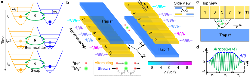
Figure 1: Coupled quantum mechanical oscillators. a, Illustration of quantum state transfer between two coupled HOs. A coherent coupling (green) fully exchanges the states of two HOs up to a phase at $t_{s}$ and creates two-mode entanglement at $t_{s}$/2, constituting a beamsplitter operation (see Supplementary Material). b, Three-dimensional perspective and c, top view of the trapping zone in a segmented Paul trap (not to scale). A ⁹Be⁺-²⁵Mg⁺-⁹Be⁺ crystal is confined along the axial direction $z$ in a harmonic potential well (solid black line in the top view). Two of three axial normal modes, “Alternating” at 3.66 MHz and “Stretch” at 3.38 MHz (mode participation vectors $\xi$ for all ions visualized as arrows in the dashed box at the bottom), are coupled by an oscillating electric potential $U({z,t})=U(z)A(t)\cos(\omega t+\phi)$. The coordinate origin is at the location of the Mg⁺ ion, and the spatial dependence of $U(z)=U_{0}z^{3}$ is visualized by the green curve in c. The potential is generated from twelve synchronized rf drives $V_{i}A(t)\cos(\omega t+\phi)$ ($i=1,...,12$, with $V_{i}$ represented by the color of wavy arrows) applied to twelve control electrodes (gold). d, Coupling pulse shape in the experiments. Green oscillating line represents the temporal dependence of $U({z,t})$ under the amplitude envelope $A(t)$ (blue dashed line).

Ideally, the timing, strength $g$, and phase $\phi$ of the coupling can be well controlled. To be practically useful, the coupling rates need to be much larger than decoherence rates of the coupled HO quantum states.

A linear string of $N$ ions confined in a three-dimensional harmonic potential and subject to mutual Coulomb repulsion exhibits $3N$ normal modes of collective ion motion that can be treated as uncoupled HOs James (1998) (see Supplementary Material). These motional modes typically have coherence times of several milliseconds and can be manipulated by external electric fields Carruthers and Nieto (1965), and by coupling to internal states of the ions using laser Wineland et al. (1998); Leibfried et al. (2003) or microwave fields Wineland et al. (1998); Mintert and Wunderlich (2001); Ospelkaus et al. (2008); Srinivas et al. (2019). In this way, individual modes can be initialized in a variety of quantum states Meekhof et al. (1996) and information about the motion can be transferred to the internal states of ions, which are in turn read out by state-dependent fluorescence Dehmelt (1982). The recoil from photons scattered during readout typically perturbs the ion motion and destroys its quantum coherence. Here, we couple pairs of normal modes by applying an electric potential with suitable spatial dependence that oscillates at the difference of two mode frequencies, and investigate the properties of such coupling operations. In particular, we can couple to a mode of motion whose symmetry protects it from perturbations during readout. This enables us to perform minimally disturbing measurements of the mode, projecting its state but not otherwise affecting it. To demonstrate this essential element of continuous-variable QEC, we repeatedly test whether the protected mode is in its ground state while preserving the state to a high degree.

We consider two normal modes $a$ and $b$ at frequencies $\omega_{a}$ and $\omega_{b}$, with position coordinates $\delta r_{n,i_{a}}$ and $\delta r_{n,i_{b}}$ referring to the displacement relative to equilibrium of the $n$th ion along direction $i_{a}$ or $i_{b}$, where $i_{a},i_{b}\in\{x,y,z\}$. To couple these modes, we apply an oscillating and spatially-varying electric potential

$$U(\boldsymbol{r},t)=U(\boldsymbol{r})A(t)\cos(\omega t+\phi),$$ (2)

with $0\leq A(t)\leq 1$ a pulse envelope (blue dashed line in Fig. 1d) that evolves slowly compared to $2\pi/\omega$, and $\omega\approx|\omega_{a}-\omega_{b}|$. The modes are coupled by curvature terms

$$\alpha_{n}=\frac{\partial^{2}U}{\partial i_{a}\partial i_{b}}|_{\boldsymbol{r}=\boldsymbol{r_{n,0}}}$$ (3)

in the expansion of $U(\boldsymbol{r})$ around the equilibrium position $\boldsymbol{r}_{n,0}$ of the $n$th ion. After transforming to the interaction picture and neglecting fast-rotating terms (see Supplementary Material), the interaction Hamiltonian has the form of Eq.(1) with $g(t)=A(t)g_{0}$. The coupling strength $g_{0}$ is a sum over contribution from each ion

$$g_{0}=\sum_{n=1}^{N}g_{n}=\sum_{n=1}^{N}\frac{Q_{n}\alpha_{n}}{4M_{n}\sqrt{\omega_{a}\omega_{b}}}\xi^{(i_{a})}_{n,a}\xi^{(i_{b})}_{n,b},$$ (4)

where $Q_{n}$, $M_{n}$, $\xi^{(i_{a})}_{n,a}$ and $\xi^{(i_{b})}_{n,b}$ denote the charge, mass and participation in modes $a$ and $b$ of the $n$th ion. The participation is defined as the $n$th ion’s component of the normalized eigenvector of a given normal mode. A particular contribution $g_{n}$ can be positive or negative and $g_{0}$ can be influenced by properly designing the curvatures $\alpha_{n}$ to constructively add when multiplied with the mode participations. For example, when two identical ions are subject to the same curvature $\alpha_{1}=\frac{\partial^{2}U}{\partial x\partial z}|_{\boldsymbol{r}=\boldsymbol{r_{1,0}}}=\alpha_{2}$, the coupling between modes $a$ and $b$, where the two ions oscillate in phase along the $z$ axis and out of phase along the $x$ axis respectively, will vanish, because $\xi^{(z)}_{1,{a}}\xi^{(x)}_{1,{b}}=-\xi^{(z)}_{2,{a}}\xi^{(x)}_{2,{b}}$. If instead the oscillating potential fulfills $\alpha_{1}=-\alpha_{2}$, the coupling terms add constructively.

Atomic motion is extremely fragile and can be significantly perturbed by a single photon recoil. However, if photon recoil can be limited to a certain ion $s$ that does not participate in a mode $a$, i.e. $\xi^{(i_{a})}_{s,a}=0$, this mode is protected and largely unperturbed even if thousands of photons are scattered from ion $s$. The coupling Eq.(1) enables “swapping” of the state in mode $a$ into a suitable mode $b$ where $\xi^{(i_{b})}_{s,b}\neq 0$ and subsequently, information about the state of $b$ can be coherently transferred to the internal state of $s$. After swapping the motional state back into $a$, readout of $s$ yields this information, while preserving the state of mode $a$ to a high degree. This could be exploited for implementing continuous-variable QEC. We characterize the degree of protection of states in the axial out-of-phase (“Stretch”) mode of a symmetric three-ion mixed species crystal from photon recoil on the middle ion (see Fig. 1b). This mode has negligible participation of the middle ion and we utilize this protection to gain information on the Stretch mode state without perturbing it substantially.

We trap ⁹Be⁺ and ²⁵Mg⁺ ions in a segmented linear Paul trap composed of two electrode layers. The structure near the trapping zone is shown in Fig. 1b and 1c (also see Blakestad (2010)). We denote the axis of the linear trap as $z$ and the two radial principal axes of the trap potential ellipsoid as $x$ and $y$. To produce the coupling potential $U(\boldsymbol{r},t)$, we apply signals oscillating at $\omega$ with different amplitudes $V_{i}$ to the twelve electrodes closest to the ions. We calculate the potentials due to each electrode to determine the set of $V_{i}$ that generates the desired curvatures at the ion positions while minimizing unwanted electric fields and curvatures. The coupling pulses have a smooth common envelope $A(t)$ applied to all electrodes that reduces sudden perturbations of the trapping potential (Fig. 1d).

We use microwave fields to implement “carrier” transitions between internal hyperfine states, which leave motional mode states unchanged. We use stimulated Raman transitions Wineland et al. (1998); Leibfried et al. (2003) on both species of ions to cool motional modes to near their ground states, to prepare approximate number states in a certain mode, and to transfer information about the states of motion onto internal states of the ions for readout by state-dependent fluorescence Meekhof et al. (1996). After near-ground-state cooling, ⁹Be⁺ is prepared in $\left|\downarrow\right\rangle_{B}\equiv\,^{2}S_{1/2}\left|F=2,m_{F}=2\right\rangle_{B}$ and ²⁵Mg⁺ in $\left|\downarrow\right\rangle_{M}\equiv\,^{2}S_{1/2}\left|F=3,m_{F}=3\right\rangle_{M}$ by optical pumping. In each experiment, information about the motional modes is mapped into the “bright” states $\left|\downarrow\right\rangle_{B}$ and $\left|\downarrow\right\rangle_{M}$. During a fluorescence detection lasting several hundred microseconds, ions in these states scatter several thousand photons in all directions, of which approximately 30 photons on average are detected, while all other hyperfine states (dark states) scatter on the order of one photon or less. Probabilities of detecting the ions to be in the “bright” and “dark” states are determined by fitting a histogram of photon counts from multiple trials to a Poisson distribution or using thresholds (see Supplementary Material). The mapping from a certain motional state to different combinations of bright and dark states is realized by $\pi$ pulses on motional sidebands or by rapid adiabatic passage (RAP) pulses Allen and Eberly (1975). Details on state mapping in each experiment are described in Supplementary Material.

Experimental characterization of the coupling between two axial modes, the “Alternating” ($\sim$3.66 MHz, subscript $A$) and Stretch ($\sim$3.38 MHz, subscript $S$) modes, in a symmetric mixed-species crystal ordered ⁹Be⁺-²⁵Mg⁺-⁹Be⁺ (BMB) as shown in Fig. 2. The participations of ions in the modes are represented by black arrows in Fig. 1b. The Mg⁺ ion does not contribute to $g_{0}$ because it has no participation in the Stretch mode. In Fig. 1c, a cubic oscillating potential $U({z,t})=A(t)U_{0}\cos(\omega t+\phi)z^{3}$ with origin at the ion crystal center (green line) yields differential (ideally opposite) $\alpha_{n}$ at the two Be⁺ ions’ positions and non-zero $g_{0}$. In a coupling pulse with a non-zero duration (Fig. 1d), $A(t)$ ramps up from zero to one in $\tau_{r}$ = 20 $\mu$s, then stays constant for $\tau_{c}$ and ramps back to zero in $\tau_{r}$. Its pulse area is equal to that of a square pulse of amplitude one and duration $\tau$ = $\tau_{r}+\tau_{c}$.

The sequence of operations for characterizing the coupling is shown in Fig. 2a. We calibrate the coupling frequency $\omega_{0}$ and strength $g_{0}$ by cooling all three axial modes close to the ground state and initializing the Alternating mode in an approximate number state $\left|n=1\right\rangle$ with a sideband $\pi$ pulse of the $\left|\downarrow\right\rangle_{M}\left|0\right\rangle_{A}\leftrightarrow\left|\uparrow\right\rangle_{M}\left|1\right\rangle_{A}$ transition ($\left|\uparrow\right\rangle_{M}\equiv\,^{2}S_{1/2}\left|F=2,m_{F}=2\right\rangle_{M}$). Exchange between the Alternating mode and Stretch mode will alter the probability that the injected phonon (motional quantum) is present in the Alternating or Stretch mode. This probability is read out through the Be⁺ ions, which participate in both modes, using a sideband pulse on the $\left|\downarrow\right\rangle_{B}\left|n\right\rangle_{A/S}\rightarrow\left|\uparrow\right\rangle_{B}\left|n-1\right\rangle_{A/S}$ transitions ($\left|\uparrow\right\rangle_{B}\equiv\,^{2}S_{1/2}\left|F=1,m_{F}=1\right\rangle_{B}$), followed by detection of state-dependent fluorescence. The probability $P(n_{A/S}=n)$ of either mode being found in number state $n$ = 0,1,2 is extracted from the observed fluorescence of the two Be⁺ ions (see Supplementary Material). When scanning the coupling pulse frequency $\omega$ (Fig. 2b) around the mode frequency difference with a fixed coupling duration of $\tau_{0}\approx$ 100$\,\mu$s, we observe a reduction of the probability $P$($n_{A}=1)$ to near zero coincident with an increase of the probability $P$($n_{S}=1)$. We next scan the pulse duration while on resonance at $\omega_{0}$ (Fig. 2c), observing $P$($n_{A}=1)$ and $P$($n_{S}=1)$ oscillating out of phase at a frequency of $\Omega_{c}=2g_{0}\approx 2\pi\times$5.1 kHz with similar contrast. The single phonon is swapped into the Stretch mode at $t_{s}\approx$ 100$\,\mu$s, and transferred back to the Alternating mode at $2t_{s}$, corresponding to a double-swap operation. The population loss per swap is estimated to be about 0.5% (see Supplementary Material). We can increase $\Omega_{c}$ to about 2$\pi\times$18 kHz, limited by low-pass filters on the electrodes and the maximum amplitude of the drive signals.

In Fig. 2d, we verify that the coupling acts as described in detail in the Supplementary Material and does not cause excess motional decoherence, by first creating a superposition $1/\sqrt{2}\left(\left|0\right\rangle_{A}+\left|1\right\rangle_{A}\right)$, followed by either a delay or a coupling pulse that results in a single swap or a double swap. Afterwards, the state of the Alternating mode is written onto the Mg⁺ internal states, followed by a microwave $\pi$/2 pulse with variable phase $\phi$. With just the delay, the whole experiment amounts to a Ramsey sequence, with a sinusoidal dependence of the probability $P(\left|\downarrow\right\rangle_{M})$ on $\phi$ (purple data points). When swapped into the Stretch mode, the motional superposition cannot be written onto the Mg⁺ ion and the subsequent $\pi/2$ pulse leads to $P(\left|\downarrow\right\rangle_{M})\approx 1/2$ independent of $\phi$ (grey data points). When double-swapped (green data points), the motional superposition returns to the Alternating mode, but also picks up an approximate phase shift of $\pi$ relative to no swap.

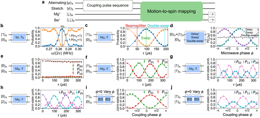
Figure 2: Coherent coupling dynamics. a, Experimental sequence for characterizing Alternating-Stretch coupling. The modes are cooled to near the ground state, then prepared in a certain state by Raman laser interactions. A coupling pulse sequence (white box) coherently exchanges the states between modes. Motional states are mapped onto one or both of the ion species by Raman laser interactions (green box, see details in text) followed by state-dependent fluorescence detection. The respective initial motional states and coupling pulse sequences (blue boxes represent single coupling pulses) are indicated in b-j. Lines in b-d are fits to the data, while lines in e-j are from numerical simulation using experimentally calibrated parameter values. b, When a single phonon is prepared in the Alternating mode, the probability of finding the phonon in the Alternating mode is high unless the coupling frequency $\omega$ is tuned near resonance, where the probability then becomes high for the phonon to be exchanged into the Stretch mode (blue squares). c, With the coupling held on resonance, a single phonon coherently swaps between the two modes as the coupling time $\tau$ increases. Vertical dashed lines in different colors indicate the pulse durations for beamsplitter (BS), swap, and double-swap operations respectively. d, Motional coherence verification after a coupling pulse. A superposition of $\left|0\right\rangle_{A}$ and $\left|1\right\rangle_{A}$ undergoes a swap operation (grey stars), a double-swap operation (teal dots), or a delay (purple squares) equivalent to the duration of the double-swap operation. Then, the motional superposition is mapped onto Mg⁺ hyperfine states $\left|\uparrow\right\rangle_{M}$ and $\left|\downarrow\right\rangle_{M}$ with a variable phase $\phi$. e-h, Probability of finding certain states in $\mathcal{S}$ as the exchange duration $\tau$ is swept for four different initial states. i,j, Phonon interference for initial states $\left|1\right\rangle_{A}\left|0\right\rangle_{S}$ and $\left|1\right\rangle_{A}\left|1\right\rangle_{S}$. Results in (f, i) and (g, j) verify two-mode entanglement generated by a beamsplitter for initial states $\left|1\right\rangle_{A}\left|0\right\rangle_{S}$ and $\left|1\right\rangle_{A}\left|1\right\rangle_{S}$ respectively. Results in (g, j) correspond to Hong-Ou-Mandel-type interference between two phonons at different frequencies.

Full characterization of entangling operations requires the detection of correlations between the entangled degrees of freedom. The distinct resonant wavelength of each ion species in the BMB crystal allows us to map joint probabilities of select number states of two normal modes onto the internal states and detect them through state-dependent fluorescence on both species. We read out the populations in the subspace $\mathcal{S}$ spanned by the nine orthonormal product states $\{\left|0\right\rangle_{A},\left|1\right\rangle_{A},\left|2\right\rangle_{A}\}\bigotimes\{\left|0\right\rangle_{S},\left|1\right\rangle_{S},\left|2\right\rangle_{S}\}$. A sideband RAP pulse maps the Stretch mode states on the two Be⁺ ions according to $\left|0\right\rangle_{S}\rightarrow\left|\downarrow\downarrow\right\rangle_{B}$, $\left|1\right\rangle_{S}\rightarrow\left|\uparrow\downarrow\right\rangle_{B}+\left|\downarrow\uparrow\right\rangle_{B}$, and $\left|2\right\rangle_{S}\rightarrow\left|\uparrow\uparrow\right\rangle_{B}$. A sequence consisting of Alternating sideband RAP pulses and microwave pulses on the Mg⁺ ion maps a chosen state among $\{\left|0\right\rangle_{A},\left|1\right\rangle_{A},\left|2\right\rangle_{A}\}$ onto the bright state $\left|\downarrow\right\rangle_{M}$, and transfers the other two number states to other hyperfine levels that appear dark during detection. Each experimental trial yields a measurement of whether or not the Alternating mode state was in the number state that was mapped to $\left|\downarrow\right\rangle_{M}$. By performing repeated experimental trials with different choices of the number state to be measured, we obtain approximate populations of all nine product states in $\mathcal{S}$ (see Supplementary Material for more details).

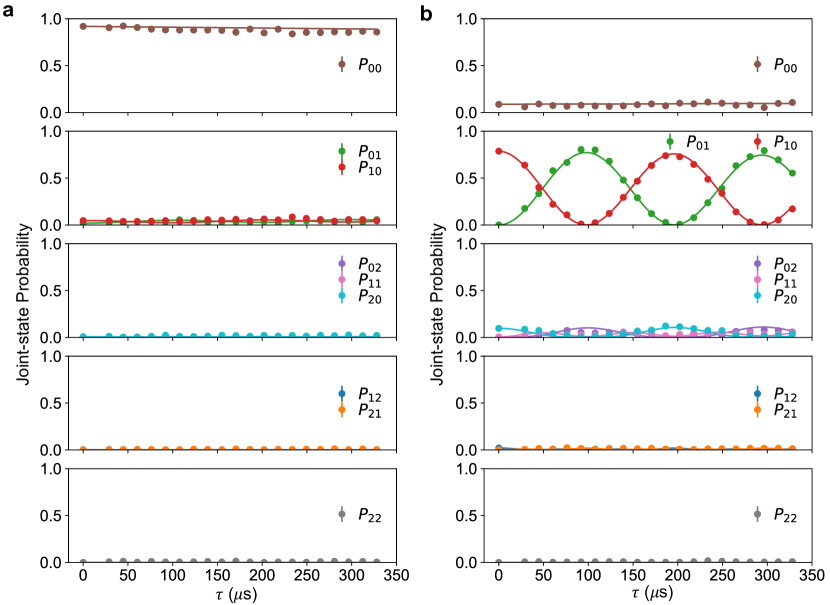
Figure 7: Joint-motional population dynamics: Coupling time scans I. The two normal modes are prepared in (a) $\left|0\right\rangle_{A}\left|0\right\rangle_{S}$ or (b) $\left|1\right\rangle_{A}\left|0\right\rangle_{S}$. The plots show population in the nine joint number states of the Alternating mode and the Stretch mode as a function of coupling time $\tau$ in five separate panels with (from top to bottom) 0 to 4 total quanta of motion in the two modes. Imperfect state preparation and measurement cause the population of the target initial state to deviate from one at $\tau$ = 0 while the other state populations may start with a non-zero value. More detailed descriptions of the experiments can be found in the main text.

Panels e-j of Fig. 2 show the correlated dynamics of the coupled modes for four initial states: $\left|n\right\rangle_{A}\left|m\right\rangle_{S}$ = {$\left|0\right\rangle_{A}\left|0\right\rangle_{S},\,\left|1\right\rangle_{A}\left|0\right\rangle_{S},\,\left|1\right\rangle_{A}\left|1\right\rangle_{S},\,\left|0\right\rangle_{A}\left|2\right\rangle_{S}\}$. The interaction Eq. (1) ideally conserves the total number $\mathcal{N}$ of motional quanta in the two modes. Experimentally, only populations of states with the same $\mathcal{N}$ were found to be substantial. These populations are shown as dots in Fig. 2e-j along with simulations (lines) Johansson et al. (2013) based on experimental parameters determined from separate measurements, including coupling strength, initial state populations, and heating rates. Dynamics of all states spanning the subspace $\mathcal{S}$ are shown in Fig. 7-10 in Supplementary Material.

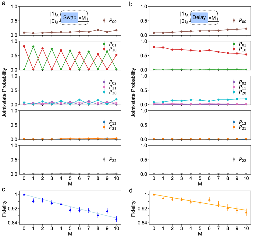
Figure 10: Joint-motional population dynamics during repeated swap operations. a, With the two modes prepared in $\left|1\right\rangle_{A}\left|0\right\rangle_{S}$, we apply M swap pulses and measure the populations of the two-mode joint states. The second panel shows that the injected single phonon is swapped between the two modes. The sum of populations in the second panel decreases as the number M of swap operations increases, while the populations of the states shown in the first and third panel grow because of heating. b, Data from a reference experiment where the coupling pulses are replaced with delays of equal duration to illustrate the effect of heating. In this case, no population is exchanged and only a slow population leakage from the initial state (red dots in the second panel) to primarily $\left|0\right\rangle_{A}\left|0\right\rangle_{S}$ (dots in the first panel) and $\left|2\right\rangle_{A}\left|0\right\rangle_{S}$ (blue dots in the third panel) is observed. This is due to a much larger heating rate in the Alternating mode compared to the Stretch mode. Solid lines in a and b serve as guides to the eye. c, With the population of all nine joint states, we estimate the fidelity of the final density matrix $\sigma$ compared to the target density matrix $\rho$ where ideal swaps are applied to an initial density matrix (data at M = 0 in a). We treat the density matrices $\sigma$ and $\rho$ as a fully decohered mixture of nine joint number states (only diagonal terms are non-zero) and estimate the fidelity with $F=(Tr\sqrt{\sqrt{\rho}\sigma\sqrt{\rho}})^{2}$. We fit the fidelities (blue triangles) to $F(\rm M)=(1-\epsilon)^{\rm M}$ to extract an error $\epsilon$ per swap operation to be 1.4(1)%. d, The same analysis is performed for the reference experiment data (orange triangles) where the fidelity to the initial density matrix (data at M = 0 in b) is shown and fitted, yielding an error per swap time of 0.9(1)%. The error of the swap operation is dominated by heating, which can be suppressed by increasing the coupling strength to reduce the swap time, or by lowering the heating rate, for example by operating in a similar trap at cryogenic temperatures.

With the system initialized in $\left|0\right\rangle_{A}\left|0\right\rangle_{S}$ ($\mathcal{N}$=0) the population mostly remains in this state, which is the only one with $\mathcal{N}$=0. We observe a slow decay out of $\left|0\right\rangle_{A}\left|0\right\rangle_{S}$ primarily due to heating of the Alternating mode (Fig. 2e), which results in the populations of $\left|0\right\rangle_{A}\left|1\right\rangle_{S}$ and $\left|1\right\rangle_{A}\left|0\right\rangle_{S}$ slowly increasing. In Fig. 2f, with $\left|1\right\rangle_{A}\left|0\right\rangle_{S}$ as the initial state ($\mathcal{N}=1$) the population swaps into the other state $\left|0\right\rangle_{A}\left|1\right\rangle_{S}$ and we observe two anti-correlated sinusoidal population oscillations with similar amplitude. The single phonon is swapped to the Stretch mode at $t_{s}$ with a population error of 1.4(1)% obtained from a separate measurement that repeatedly applies swap pulses (see error estimation in Fig. 10 in Supplementary Material). At $t_{BS}$ $\approx$ 50 $\mu$s, the coupling pulse realizes a beamsplitter (BS) operation $U=\exp[i(\pi/4)(\hat{a}\hat{b}^{\dagger}+\hat{b}\hat{a}^{\dagger})]$, which we expect to generate a NOON-type entangled motional state $\frac{1}{\sqrt{2}}(\left|1\right\rangle_{A}\left|0\right\rangle_{S}+\left|0\right\rangle_{A}\left|1\right\rangle_{S})$ Sanders (1989). We observe approximately equal population in $\left|0\right\rangle_{A}\left|1\right\rangle_{S}$ and $\left|1\right\rangle_{A}\left|0\right\rangle_{S}$ at $t_{BS}$ and verify the coherence between these two components by performing a phonon interferometry experiment consisting of two BS operations with variable phase difference $\phi$. The resulting interference fringes are shown in Fig. 2i and have similar contrast as the time scan data in Fig. 2f, indicating that motional coherence is preserved and an approximate NOON state is generated by the first BS pulse.

The initial state $\left|1\right\rangle_{A}\left|1\right\rangle_{S}$ evolves into $\left|0\right\rangle_{A}\left|2\right\rangle_{S}$ and $\left|2\right\rangle_{A}\left|0\right\rangle_{S}$ with nearly equal population, while the population in $\left|1\right\rangle_{A}\left|1\right\rangle_{S}$ is reduced almost to zero at $t_{BS}$ by destructive interference (Fig. 2g). This behavior is analogous to Hong–Ou–Mandel (HOM) interference Hong et al. (1987); here the interference is between phonons at different frequencies. The NOON state $\frac{1}{\sqrt{2}}(\left|2\right\rangle_{A}\left|0\right\rangle_{S}+\left|0\right\rangle_{A}\left|2\right\rangle_{S})$ is generated at $t_{BS}$, and the phase coherence of this state is also verified by a phonon interferometry experiment (Fig. 2j). When $\left|0\right\rangle_{A}\left|2\right\rangle_{S}$ is prepared (Fig. 2h), the two phonons are almost fully transferred into the Alternating mode ($\left|2\right\rangle_{A}\left|0\right\rangle_{S}$) at $t_{s}$, but they also partially populate $\left|1\right\rangle_{A}\left|1\right\rangle_{S}$ for $0<t<t_{s}$.

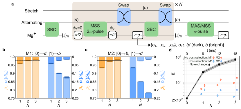
Figure 3: Repeated measurements of quantum ground state of trapped-ion motion. a, Diagram of measurement for non-destructively distinguishing number states $\{\left|0\right\rangle$, $\left|1\right\rangle\}$. The Alternating mode is initialized in a thermal distribution at $\bar{n}$ = 0.023(1), with $>0.999$ of the population in $\left|0\right\rangle$ ($p_{0}$=0.978(1)) and $\left|1\right\rangle$ ($p_{1}$=0.022(1)). These states can be distinguished with the operations in the grey box (see text) and read out on Mg⁺ after swapping the motional state into the Stretch mode to protect it from the recoil of the Mg⁺ ion during detection and sideband cooling (SBC). Another swap pulse brings the motional state back to the Alternating mode such that this measurement can be repeated. In each repetition, Mg⁺ is declared either bright ($b$) or dark ($d$) by comparing the detected photon number with a threshold of nine. We obtain a series of binary outcomes $\{o_{1},...,o_{i},...,o_{N}\}$, $o_{i}\in\{d,b\}$ with the measurement performed $N$ times. When $\phi_{2}=0$, we realize the mapping (M1): $\left|0\right\rangle\rightarrow d$, $\left|1\right\rangle\rightarrow b$, while $\phi_{2}=\pi$ exchanges the roles of $b$ and $d$, (M2): $\left|1\right\rangle\rightarrow d$, $\left|0\right\rangle\rightarrow b$. We verify the motional state after a certain sequence by measuring MAS and MSS excitation. b and c, Repeated measurement outcomes match the initial distribution. For M1 (b), we declare the state is $|0\rangle$ ($|1\rangle$) if all $N$ outcomes are $d$ ($b$), which occurs with probability $p(\{d\}_{N})$ ($p(\{b\}_{N})$). The relative frequencies of finding $|0\rangle$ and $|1\rangle$, {$\tilde{p}_{0}$ (light orange bars), $\tilde{p}_{1}$ (dark orange bars)} extracted (see text) from $p(\{d\}_{N})$ (light blue bars) and $p(\{b\}_{N})$ (dark blue bars), are consistent with {$p_{0}$, $p_{1}$} (dashed line). As $N$ increases, $\{\tilde{p}_{0},\tilde{p}_{1}\}$ become closer to the initial distribution but use less data, $i.e.$ the sum of $p(\{d\}_{N})$ and $p(\{b\}_{N})$ decreases. For M2 (c), we identify the state as $|0\rangle$ or $|1\rangle$ if all $N$ outcomes are $b$ or $d$ and observe similar results. d, Alternating mean occupation number ($\bar{n}$) post-selected on all $N$ outcomes being $d$ for M1 (blue dots) or $b$ for M2 (blue diamonds) are lower than the corresponding $\bar{n}$ with no post-selection (red symbols). “No exchange” $\bar{n}$ (black squares), which are measured after applying a delay with the duration of $N$ measurement blocks without swapping into the Stretch mode, are substantially higher than other results due to the higher heating rate of the Alternating mode. Data points are laterally offset from nominal $N$ values for legibility and error bars for some points are smaller than the plot symbols.

High-fidelity swap operations between the protected Stretch mode and the Alternating mode, the latter of which has substantial participation of the Mg⁺ ion, allow us to write information about a motional state in the Alternating mode onto Mg⁺ and then swap the motional state into the Stretch mode to preserve it during readout of the Mg⁺ ion. Preservation of the motional state enables the measurement to be repeated to achieve greater confidence in the result. Here, we implement a measurement that can non-destructively distinguish a number state $\left|n\right\rangle\in\{\left|0\right\rangle$, $\left|1\right\rangle\}$ of ion motion using the circuit shown in Fig. 3a. While $\left|n\right\rangle$ is stored in the Alternating mode, information can be mapped onto the Mg⁺ internal state with a Cirac-Zoller sequence (schematically shown in grey box, see Supplementary Material for details) that contains a motion-subtracting-sideband (MSS) 2$\pi$ pulse surrounded by two carrier $\pi/2$ pulses. This MSS pulse ideally will leave both $\left|0\right\rangle$ and $\left|1\right\rangle$ unaffected and will introduce a $\pi$ phase shift between the internal states only when the motional state is $\left|1\right\rangle$ Cirac and Zoller (1995). When the phase of the second $\pi/2$ pulse $\phi_{2}$ = 0, we map $\left|0\right\rangle$ and $\left|1\right\rangle$ to a dark ($d$) and bright ($b$) state respectively, $i.e.$ $\left|0\right\rangle\rightarrow d$ and $\left|1\right\rangle\rightarrow b$, and we label this mapping as M1. By setting $\phi_{2}=\pi$, we realize $\left|0\right\rangle\rightarrow b$ and $\left|1\right\rangle\rightarrow d$, labelled as M2. The state $\left|n\right\rangle$ is swapped to the Stretch mode before Mg⁺ fluorescence detection. Due to the limited collection and detection efficiency of our apparatus, we detect approximately 30 photons on average when in the bright state, while the total number of photons scattered into all directions is several thousand. In each measurement, we declare the Mg⁺ ion to be bright or dark depending on whether or not the number of detected photons is greater than nine. The in-phase (INPH) mode and the Alternating mode are cooled to near their ground states and another swap pulse transfers the number state back to the Alternating mode to permit the next measurement. This particular measurement cannot distinguish number states with $n>1$, but can be adapted in principle to reveal any single bit of information about the state of the motion by simply modifying the mapping sequence, which may make it amenable to syndrome extraction in bosonic error correction codes Chuang et al. (1997); Gottesman et al. (2001); Leghtas et al. (2013); Michael et al. (2016).

As a demonstration, the Alternating mode is sideband cooled to a thermal distribution with an average occupation of $\bar{n}$ = 0.023(1), with more than 99.9% of the population in $\left|0\right\rangle$ ($p_{0}$=0.978(1)) and $\left|1\right\rangle$ ($p_{1}$=0.022(1)). We repeat the motional state measurement up to three times and obtain a series of outcomes $\{o_{1},...,o_{i},...,o_{N}\}$ with $o_{i}\in\{d,b\}$, $i$=1,…, $N$. For M1, we declare the state is $\left|0\right\rangle$ or $\left|1\right\rangle$ if all $N$ outcomes are the same (all $d$ or all $b$, respectively), and discard the other outcomes because the state is not distinguished faithfully. The relative frequencies of finding $\left|0\right\rangle$ and $\left|1\right\rangle$, defined as $\tilde{p}_{0}=p(\{d\}_{N})/(p(\{d\}_{N})+p(\{b\}_{N})$ and $\tilde{p}_{1}=1-\tilde{p}_{0}$, should match with the initial distribution $\{p_{0},p_{1}\}$, where $p(\{d\}_{N})$ and $p(\{b\}_{N})$ are the probabilities of all $N$ outcomes being $d$ and $b$ respectively. For M2, the roles of $d$ and $b$ are exchanged. We examine the final state of the Alternating mode by applying a $\pi$ pulse on the motion-adding-sideband (MAS) transition $\left|\downarrow\right\rangle_{M}\left|0\right\rangle\leftrightarrow\left|\uparrow\right\rangle_{M}\left|1\right\rangle$ or a pulse of the same duration on the MSS transition, followed by Mg⁺ fluorescence detection. The $\bar{n}$ conditioned on various measurement outcomes can be estimated with MAS and MSS transition probabilities, if the conditioned state is close to a thermal state, or if the population is predominantly in $\left|0\right\rangle$ and $\left|1\right\rangle$ Leibfried et al. (2003).

In Fig. 3b, using M1 and $N$=1, we detect $\{d\}$ heralding $|0\rangle$ and obtain $\tilde{p}_{0}$ (light orange bar)= $p(\{d\})_{N=1}$ (light blue bar)= 0.960(3) while $\tilde{p}_{1}$ (dark orange bar)= $p(\{b\})_{N=1}$ (dark blue bar) = 0.040(3). The {$\tilde{p}_{0}$, $\tilde{p}_{1}$} are close to the initial state populations {$p_{0},p_{1}$} (indicated by dashed line) respectively with a small difference of about 0.02, which indicates a detection error. With $N$ = 2, the {$\tilde{p}_{0}$, $\tilde{p}_{1}$} are only different from {$p_{0}$, $p_{1}$} by 0.002(2) because the state is heralded twice, largely suppressing erroneous declarations. However, we discard about 7.8% of the total trials (gap between light blue and dark blue bars) where the outcomes from the two rounds disagree. This number is larger than the detection error of a single round, indicating that the motional state is slightly changed during the measurements, likely due to heating. With $N$ = 3, the $\{\tilde{p}_{0},\tilde{p}_{1}\}$ are also close to the initial distribution, but another 3% of the total trials are discarded. In Fig. 3c, we implemented M2 and observed that $\{\tilde{p}_{0},\tilde{p}_{1}\}$ also match well with the initial distribution. Compared to M1, more data were discarded due to disagreement between repeated measurements, suggesting that Mg⁺ scattering may introduce additional disturbance to the motional state. For larger $N$ with either M1 or M2, the leakage into higher number states also increases because of heating and may lower the readout fidelity.

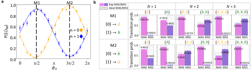
Figure 12: Cirac-Zoller mapping phase calibration and sideband transition probabilities conditioned on different motional state measurement outcomes. a, With the Alternating mode prepared in $\left|0\right\rangle_{A}$ (orange) or $\left|1\right\rangle_{A}$ (blue), we obtain two sinusoidal curves that oscillate out of phase as a function of the phase $\phi_{2}$ of the second $\pi$/2 pulse relative to the first $\pi$/2 pulse in the CZ sequence. The two vertical dashed lines indicate the phases for realizing mappings M1 and M2. b, MAS and MSS transition probabilities conditioned on the outcomes shown above each panel; measurements are repeated $N$ = 1, 2, 3 times under both M1 and M2. The grey hatched bars denote the ideal probabilities for $\left|0\right\rangle$ and $\left|1\right\rangle$ which are compared with experimental results (colored bars). For M1 (M2), when $|0\rangle$ is heralded by detecting $d$ ($b$) $N$=1, 2, 3 times, the sideband results match well with the ideal values. When $|1\rangle$ is heralded once ($N$=1), the sideband results deviate significantly from the ideal values for $|1\rangle$ because of false declaration events for $|0\rangle$ (see text in Supplementary Material). After performing the measurement more times ($N$=2 and 3), the sideband results when $|1\rangle$ is heralded are substantially closer to the ideal expectation values because the detection error is reduced.

The $\bar{n}$ values of final motional states as determined by MAS/MSS transition rates are shown in Fig. 3d. The black data points represent $\bar{n}$ after waiting an equivalent duration as is required for mapping, swapping, readout and cooling during the repeated measurement blocks. The increase in $\bar{n}$ is predominantly due to heating of the Alternating mode. The red dots and red diamonds represent trials where the measurement blocks are executed with mapping M1 and M2 respectively, but no further action is taken before determining $\bar{n}$. The $\bar{n}$ values are reduced compared to the black points because of the lower heating rate in the Stretch mode, where the motional state is stored part of the time. The remaining data show $\bar{n}$ post-selected on the measurement heralding $\left|0\right\rangle$ $N$ times. The blue dots are for M1 and the blue diamonds for M2. In all cases, M1—where $\left|0\right\rangle$ is heralded by no photons scattered on Mg⁺—yields the lowest $\bar{n}$. However, the case post-selected on scattering photons when in $\left|0\right\rangle$ (M2) also yields lower $\bar{n}$ than the unconditioned data. This shows that the measurements where photons are scattered do not perfectly preserve the motional state, but still yield useful information and can keep the state closer to the ideal outcome despite many recoils suffered by the Mg⁺ ion during readout. The difference between using M1 and M2 is likely due to a small amount of recoil heating in the Stretch mode, caused by non-ideal odd anharmonic terms in the trapping potential (see Supplementary Material). Complete MAS and MSS results for all $N$ and all outcomes can be found in Table 1-3 and Fig. 12b in Supplementary Material.

Coherent coupling of normal modes of a mixed-species ion string can be applied for cooling et.al. , indirect state preparation Chou et al. (2017), and precision spectroscopy of charged particles based on quantum logic Schmidt et al. (2005). The required time-varying potentials couple to the charge of the particles only, leaving electronic and spin states unaffected to a high degree. The coupling remains robust over weeks with very little calibration in our setup and can be enhanced and refined in smaller traps with more control electrodes. Coherent mode coupling can extend existing techniques, such as providing two-mode operations for continuous-variable quantum computing Lloyd and Braunstein (1999). Higher-order coupling potentials permit Kerr-type couplings Roos et al. (2008); Ding et al. (2017) or can act on more than two modes simultaneously. Any of these techniques can be combined with well-developed spin-motion control techniques to enable simulations of more complicated physical models Hartmann et al. (2006); Greentree et al. (2006). Protected modes can be exploited for more general measurements that leave a motional state intact. We note that similar work on protected modes of trapped ion crystals is underway in other research groups Metzner et al. (2021).

Supplementary Material: Coherently coupled mechanical oscillators in the quantum regime

I Coupling Hamiltonian derivation

We consider a mixed-species linear string consisting of $N$ ions with different masses $M_{n}$ and charges $Q_{n}$ $(n=1,...,N)$, trapped in a three-dimensional potential well $U_{0}(\textbf{r})$. We choose a coordinate system that is aligned with the principal axes of the equipotential ellipsoids that characterize $U_{0}(\textbf{r})$ near its minimum position, which we define as the origin of the coordinate system. As shown in Fig. 1b, $x$ and $y$ are defined by the control and rf electrodes, and $z$ is along the trap axis which runs parallel to the electrode edges. The coordinate origin is in the plane parallel to and midway between the electrode wafers and coincides with the minimum of the harmonic potential (black line) sketched in Fig. 1c. The coordinate axes line up with the eigenvectors of three groups of normal (decoupled) motional modes, with $N$ modes in each group that we will derive next. The total potential energy summed over ions at positions $\textbf{r}_{n}=(r_{x,n},r_{y,n},r_{z,n})^{T}$ is given by

$$U_{pot}(\textbf{r}_{1},...\textbf{r}_{N})=\sum_{n=1}^{N}Q_{n}U_{0}(\textbf{r}_{n})+\sum_{n=1}^{N}\sum_{n^{\prime}=n+1}^{N}\frac{Q_{n}Q_{n^{{}^{\prime}}}}{4\pi\epsilon_{0}|\textbf{r}_{n}-\textbf{r}_{n^{{}^{\prime}}}|}.$$ (5)

By solving $\partial U_{pot}/\partial\textbf{r}_{n}=0$, we obtain each ion’s equilibrium position $\textbf{r}_{n}^{(0)}$. Expanding $U_{pot}$ to second-order in small, mass-weighted coordinate changes $q_{i,n}=(r_{i,n}-r_{i,n}^{(0)})/\sqrt{M_{n}}$ with $i\in\{x,y,z\}$ around $\textbf{r}_{n}^{(0)}$ and diagonalizing the resulting Hessian matrix, we obtain $3N$ mutually decoupled normal modes of ion motion with frequencies $\omega_{i,m}$ and quantized normal mode coordinates

$$u_{i,m}=\sqrt{\frac{\hbar}{2\omega_{i,m}}}\left(\hat{a}_{i,m}+\hat{a}^{\dagger}_{i,m}\right),$$

where $\omega_{i,m}$, $\hat{a}^{\dagger}_{i,m}$, and $\hat{a}_{i,m}$ are the motional frequency, creation operator, and annihilation operator respectively of the $m$-th mode along axis $i\,\in\,\{x,y,z\}$. In the normal mode coordinates, the Hamiltonian of the motion of an ion string consists of $3N$ uncoupled HOs and can be written as

$$H_{0}=\sum_{i\in\{x,y,z\}}\sum_{m=1}^{N}\hbar\omega_{i,m}\left(\hat{a}^{\dagger}_{i,m}\hat{a}_{i,m}+1/2\right).$$

Each ion oscillates around its equilibrium position, but does not participate in all normal modes equally in general and may not participate at all in some modes. For the $n$th ion the displacement along the $i$-th axis, $\hat{q}_{i,n}$ can be written in terms of the $m$-th normal mode creation and annihilation operators as

$$\hat{q}_{i,n}=\sum^{N}_{m=1}\sqrt{\frac{\hbar}{2M_{n}\omega_{i,m}}}\xi^{(i)}_{n,m}\left(\hat{a}_{i,m}+\hat{a}_{i,m}^{\dagger}\right),$$ (6)

where $\xi^{(i)}_{n,m}$ is the transformation matrix element between the spatial coordinates of the $n$th ion displacement $q_{i,n}$ along axis $i$ and the normal mode vector component along the same axis for the $m$-th eigenmode.

To couple two particular normal modes, mode $a$ oscillating at frequency $\omega_{i_{a},a}$ along axis $i_{a}$ and mode $b$ at frequency $\omega_{i_{b},b}$ along axis $i_{b}$, we can apply an oscillating perturbing potential $U_{\rm pert}(\textbf{r},t)=U(\textbf{r})\cos(\omega t+\phi)$ with $\omega$ close to the frequency difference of the modes we would like to couple, $\omega\approx\omega_{i_{a},a}-\omega_{i_{b},b}$. Expanding $U(\textbf{r})$ up to second-order around a certain position $\textbf{r}_{0}$, we obtain

$$U(\textbf{r}_{0}+\delta\textbf{r})\approx U(\textbf{r}_{0})+\sum_{i\in\{x,y,z\}}\frac{\partial U}{\partial i}|_{\boldsymbol{r}=\boldsymbol{r}_{0}}\delta r_{i}+\frac{1}{2}\sum_{i,j\in\{x,y,z\}}\frac{\partial^{2}U}{\partial i\partial j}|_{\textbf{r}=\textbf{r}_{0}}\delta r_{i}\delta r_{j}.$$ (7)

Anticipating that only terms proportional to $\delta r_{i_{a}}\delta r_{i_{b}}$ of the two normal modes we desire to couple will rotate slowly in the interaction picture with respect to $H_{0}$, we can drop all other terms in $U(\textbf{r})$ to simplify the following steps,

$$U(\textbf{r}_{0}+\delta\textbf{r})\approx 2^{-\delta(i_{a},i_{b})}\frac{\partial^{2}U}{\partial i_{a}\partial i_{b}}|_{\textbf{r}=\textbf{r}_{0}}\delta r_{i_{a}}\delta r_{i_{b}},$$

where $\delta(i_{a},i_{b})=1$ for $i_{a}=i_{b}$ and 0 otherwise and we have used $\partial^{2}U/(\partial i_{a}\partial i_{b})=\partial^{2}U/(\partial i_{b}\partial i_{a})$. In practice, the dropped terms may cause undesirable distortion of the potential and excess ion motion and should be minimized when designing the perturbing potential. Again only keeping near-resonant terms, inserting the displacement operators for displacements of the $n$th ion in modes $a,b$, namely $\delta r_{i_{a},n}=\hat{q}_{i_{a},n},\delta r_{i_{b},n}=\hat{q}_{i_{b},n}$, abbreviating $\partial^{2}U/(\partial i_{a}\partial i_{b})|_{\boldsymbol{r}=\boldsymbol{r^{(0)}_{n}}}=\alpha_{n}$ and inserting Eq. (6), the Hamiltonian from the perturbing potential can be approximated as

$$\begin{split}H=&\sum_{n=1}^{N}Q_{n}U_{\rm pert}(\textbf{r}_{n},t)\\ \approx&\sum_{n=1}^{N}Q_{n}2^{-\delta(i_{a},i_{b})}\alpha_{n}\hat{q}_{i_{a},n}\hat{q}_{i_{b},n}\cos(\omega t+\phi)\\ =&\sum_{n=1}^{N}Q_{n}2^{-\delta(i_{a},i_{b})}\alpha_{n}\left[\sum_{m=1}^{N}\sqrt{\frac{\hbar}{2M_{n}\omega_{i_{a},m}}}\xi^{(i_{a})}_{n,m}\left(\hat{a}_{i_{a},m}+\hat{a}_{i_{a},m}^{\dagger}\right)\right]\\ &\qquad\times\left[\sum_{l=1}^{N}\sqrt{\frac{\hbar}{2M_{n}\omega_{i_{b},l}}}\xi^{(i_{b})}_{n,l}\left(\hat{a}_{i_{b},l}+\hat{a}_{i_{b},l}^{\dagger}\right)\right]\\ &\qquad\times\frac{1}{2}\left(e^{-i(\omega t+\phi)}+e^{i(\omega t+\phi)}\right)\\ =&\sum_{n,m,l=1}^{N}2^{-\delta(i_{a},i_{b})}\frac{\hbar Q_{n}\alpha_{n}}{4M_{n}\sqrt{\omega_{i_{a},m}\omega_{i_{b},l}}}\xi^{(i_{a})}_{n,m}\xi^{(i_{b})}_{n,l}\left(\hat{a}_{i_{a},m}+\hat{a}_{i_{a},m}^{\dagger}\right)\left(\hat{a}_{i_{b},l}+\hat{a}_{i_{b},l}^{\dagger}\right)\left(e^{-i(\omega t+\phi)}+e^{i(\omega t+\phi)}\right).\end{split}$$ (8)

We analyze this expression in the interaction frame with respect to $H_{0}$ by replacing $\hat{a}_{i,m}\rightarrow\hat{a}_{i,m}e^{-i\omega_{i,m}t}$, $\hat{a}_{i,m}^{\dagger}\rightarrow\hat{a}_{i,m}e^{i\omega_{i,m}t}$. When $\omega\approx\omega_{i_{a},a}-\omega_{i_{b},b}$, we can neglect all terms that are not rotating at $\pm\left[\omega-\left(\omega_{i_{a},a}-\omega_{i_{b},b}\right)\right]$, which simplifies the coupling Hamiltonian (8) to

$$H=\hbar g_{0}\left(e^{i\phi}\hat{a}\hat{b}^{\dagger}+e^{-i\phi}\hat{a}^{\dagger}\hat{b}\right)$$ (9)

where we use $\omega_{i_{a},a}=\omega_{a}$, $\omega_{i_{b},b}=\omega_{b}$, $\hat{a}_{i_{a},a}=\hat{a}$ and $\hat{a}_{i_{b},b}=\hat{b}$ for simplicity from this point onward. Note that coupling two modes along the same axis, $i_{a}=i_{b}$, results in two near-resonant cross-terms proportional to $\xi^{(i_{a})}_{n,a}\xi^{(i_{a})}_{n,b}$ and $\xi^{(i_{a})}_{n,b}\xi^{(i_{a})}_{n,a}$ that both contribute to the coupling equally and cancel the factor $2^{-\delta(i_{a},i_{a})}$. The coupling strength is

$$g_{0}=\sum_{n=1}^{N}g_{n}=\sum_{n=1}^{N}\frac{Q_{n}\alpha_{n}}{4M_{n}\sqrt{\omega_{a}\omega_{b}}}\xi^{(i_{a})}_{n,a}\xi^{(i_{b})}_{n,b}.$$ (10)

This is identical to Eq. (4) in the main text.

II Time evolution of coupled motional states

When two modes represented by ladder operators $\hat{a}$ and $\hat{b}$ are coupled by the Hamiltonian Eq.(9), their states of motion will become entangled and, after an exchange of population, disentangled, in a periodic fashion. The time-dependent states can be found by first performing a basis transformation

$$\hat{c}_{+} = \frac{1}{\sqrt{2}}\left(\hat{a}+e^{-i\phi}\hat{b}\right)$$

$$\hat{c}_{-} = \frac{1}{\sqrt{2}}\left(\hat{a}-e^{-i\phi}\hat{b}\right),$$ (11)

which diagonalizes the interaction Hamiltonian

$$\hbar g_{0}\left(e^{i\phi}\hat{a}\hat{b}^{\dagger}+e^{-i\phi}\hat{a}^{\dagger}\hat{b}\right)=\hbar g_{0}\left(\hat{c}_{+}^{\dagger}\hat{c}_{+}-\hat{c}_{-}^{\dagger}\hat{c}_{-}\right).$$ (12)

The right hand side represents two harmonic oscillators with energies separated by twice the interaction energy $\hbar g_{0}$. In the interaction frame of reference, these oscillators have simple equations of motion

$$\hat{c}^{\dagger}_{\pm}(t)=\hat{c}^{\dagger}_{\pm}(0)\exp(\pm ig_{0}t).$$ (13)

Writing $\hat{a}^{{\dagger}}(0)=\hat{a}^{{\dagger}}$, $\hat{b}^{{\dagger}}(0)=\hat{b}^{{\dagger}}$ for brevity and inserting the time dependence into the equations for $\hat{a}(t)$ and $\hat{b}(t)$ yields

$$\hat{a}^{\dagger}(t) = \hat{a}^{\dagger}\cos(g_{0}t)+ie^{i\phi}\hat{b}^{\dagger}\sin(g_{0}t)$$

$$\hat{b}^{\dagger}(t) = \hat{b}^{\dagger}\cos(g_{0}t)+ie^{-i\phi}\hat{a}^{\dagger}\sin(g_{0}t).$$ (14)

Any state of the oscillators at time $t$ can be written as a superposition of number states with complex amplitudes $c_{mn}$ by acting with different combinations of creation operators on the vacuum state $\left|0\right\rangle_{a}\left|0\right\rangle_{b}$,

$$\left|\Psi_{a}(t)\right\rangle\left|\Phi_{b}(t)\right\rangle=\sum_{m,n=0}^{\infty}\frac{c_{mn}}{\sqrt{m!n!}}\left[\hat{a}^{\dagger}(t)\right]^{m}\left[\hat{b}^{\dagger}(t)\right]^{n}\left|0\right\rangle_{a}\left|0\right\rangle_{b},$$ (15)

such that the time dependence is fully captured in the creation operators. For general times $t$ this implies a rather complicated entangled state of the modes, which becomes simpler for certain evolution times. For example when setting $\tau_{\rm BS}=\pi/(4g_{0})$ the trigonometric factors $\sin(g_{0}\tau_{\rm BS})=\cos(g_{0}\tau_{\rm BS})=1/\sqrt{2}$ and Eq.(II) turns into a beamsplitter relation Caves (1981) that can be used to demonstrate the Hong-Ou-Mandel effect, here for two modes at different frequencies in a mixed-species string of ions (See the main text and Fig. 2g and 2j).

Eq.(II) simplifies even more for $\tau_{k}=k\pi/(2g_{0})$ with $k$ a positive integer. For $k$ odd this yields

$$\hat{a}^{\dagger}(\tau_{k}) = ie^{i(g_{0}\tau_{k}+\phi)}\hat{b}^{\dagger}$$

$$\hat{b}^{\dagger}(\tau_{k}) = ie^{i(g_{0}\tau_{k}-\phi)}\hat{a}^{\dagger},$$ (16)

which implies that $\left|\Psi_{a}(\tau_{k})\right\rangle\left|\Phi_{b}(\tau_{k})\right\rangle$ with $k$ odd has the original states of modes $a$ and $b$ swapped and shifted by a phase $g_{0}\tau_{k}\pm\phi$. This phase difference arises relative to that of the uncoupled evolution of the modes and can be thought of as a consequence of the coupling that modifies the energies of the eigenstates with the additional factors due to the phase $\phi$ of the applied drive. For $k$ even

$$\hat{a}^{\dagger}(\tau_{k}) = e^{ig_{0}\tau_{k}}\hat{a}^{\dagger}$$

$$\hat{b}^{\dagger}(\tau_{k}) = e^{ig_{0}\tau_{k}}\hat{b}^{\dagger},$$ (17)

which signifies one or several complete forth-and-back exchanges and a phase shift due to the coupling energy. Up to this phase shift, the state $\left|\Psi_{a}(\tau_{k})\right\rangle\left|\Phi_{b}(\tau_{k})\right\rangle$ with $k$ even is identical to the one at $t=0$ in the interaction frame of reference.

III Experimental methods

Coupling drive generation and control
We use a segmented linear Paul trap consisting of a pair of RF electrodes and 47 control electrodes Blakestad (2010). The voltages of the control electrodes are produced by 47 independent arbitrary waveform generators (AWGs) with a 50 MHz clock rate Bowler et al. (2013). Each AWG output is connected to a control electrode through a two-stage low-pass filter with a 3 dB corner frequency of about 50 kHz to suppress noise at motional frequencies. The oscillating potential $U(\textbf{r},t)$ for creating mode-mode coupling is produced by the twelve electrodes nearest to the ions controlled by their AWGs. The oscillating signals are added to the static voltages that produce the axial confinement. The AWGs are not actively synchronized, but have approximately equal clock speeds, so we reset their phase at the beginning of each experiment to make sure all the drives oscillate in phase. Coupling of motional modes becomes ineffective for motional frequency differences larger than 1 MHz due to attenuation from the low-pass filters and the 1 MHz bandwidth of the AWG output amplifiers.

We shape the amplitude envelope of coupling pulses to suppress the excitation of nearby normal modes due to spectral side-lobes of square pulses. The pulse amplitude ramps up as approximately $\sin(2\pi ft)^{2}$ (with $f$= 12.5 kHz and 0 $\leq t\leq$ 20 $\mu$s) at the beginning of the pulse and ramps back to zero using the time-reversal of the ramp-up. We observe significant off-resonant excitation of the axial in-phase mode (at $\sim$ 1.5 MHz) of a BMB crystal when using a square coupling pulse around the resonant frequency of the Alternating-Stretch coupling, while such excitation is largely suppressed with shaped pulses.

We determine the coupling drive amplitudes for the twelve electrodes using a trap potential simulation Blakestad (2010) to generate a potential for which the desired spatial derivative is maximized while the unwanted components are minimized. These unwanted terms typically include the gradients $\partial U/\partial i$, $i\in\{x,y,z\}$, which displace and potentially heat the ion motion, and the curvatures $\partial^{2}U/\partial i^{2}$, $i\in\{x,y,z\}$ which modulate motional frequencies. Higher-order derivatives of the potential are typically negligible in our trap and are not considered in the simulations.

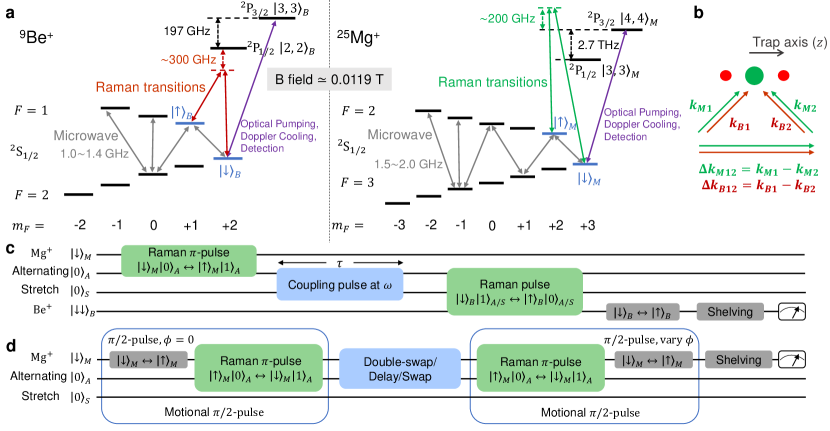
Figure 4: a, Relevant electronic states of ⁹Be⁺ and ²⁵Mg⁺ at an applied magnetic quantization field of $|\vec{B}|\approx$ 0.0119 T. b, Configuration of Raman laser beams for Be⁺ (red) and Mg⁺ (green). c, Experimental sequence for calibrating coupling resonant frequency and rates (results in Fig. 2b,c) of the Alternating-Stretch coupling. d, Experimental sequence for a motional Ramsey interference experiment between $\left|0\right\rangle_{A}$ and $\left|1\right\rangle_{A}$ (results in Fig. 2d) with a delay, or a coupling pulse for a single swap or a double swap inserted between the motional $\pi/2$ pulses.

Ion species and state manipulation
We trap two ion species, ⁹Be⁺ and ²⁵Mg⁺, at a quantization magnetic field of $\sim$ 0.0119 T. The relevant electronic states of both species are illustrated in Fig. 4a. A $\sigma^{+}$-polarized ultraviolet (UV) laser beam near 313 nm optically pumps Be⁺ ions to $\left|\downarrow\right\rangle_{B}=$ ${}^{2}S_{1/2}\left|F=2,m_{F}=2\right\rangle_{B}$, while Doppler cooling and state-dependent fluorescence detection are implemented with a second UV laser beam driving the ${}^{2}S_{1/2}\left|2,2\right\rangle_{B}\leftrightarrow\,^{2}P_{3/2}\left|3,3\right\rangle_{B}$ cycling transition, causing photons to be emitted from the ion when Be⁺ is in the “bright” state $\left|\downarrow\right\rangle_{B}$. Similarly, Mg⁺ ions are optically pumped to the bright state $\left|\downarrow\right\rangle_{M}$= ${}^{2}S_{1/2}\left|3,3\right\rangle_{M}$ with a $\sigma^{+}$-polarized laser beam near 280 nm. A second UV laser beam is used to drive the ${}^{2}S_{1/2}\left|3,3\right\rangle_{M}\leftrightarrow\,^{2}P_{3/2}\left|4,4\right\rangle_{M}$ transition for Doppler cooling and fluorescence detection.

State-dependent fluorescence detection is accomplished with resonant UV light illuminating the ions for a duration of 330 $\mu$s for Be⁺ and 200 $\mu$s for Mg⁺, with a fraction of the ion fluorescence collected by an achromatic imaging system and detected by a photomultiplier tube. To distinguish two hyperfine states of interest, we apply a “shelving” sequence that consists of microwave $\pi$ pulses to transfer one hyperfine state to the bright state and the other to a dark state (a hyperfine state away from the bright state in the ${}^{2}S_{1/2}$ manifold) before fluorescence detection. The microwave transitions used in the shelving sequence are indicated with grey double-arrows in Fig. 4a. The detected photon counts approximately follow Poisson distributions with a mean of $\sim$ 30 counts for each ion when they are in the bright states $\left|\downarrow\right\rangle_{B}$ and $\left|\downarrow\right\rangle_{M}$. The ions scatter only a few photons per detection when in any other hyperfine states. In particular, we detect a background of $\sim$ 2 photons for Be⁺ and $\sim$ 1 photons for Mg⁺ (dominated by background scatter) when ions are in the “dark” states, ${}^{2}S_{1/2}\left|1,-1\right\rangle_{B}$ and ${}^{2}S_{1/2}\left|2,-2\right\rangle_{M}$.

In the coupling calibrations, we analyze the photon counts of a reference dataset by using maximum likelihood estimation (MLE) to determine the Poissonian mean photon counts of $N$= 0,1,2 Be⁺ ions in the bright state. Then, we determine the probability $P_{b}(N)$ of $N$ Be⁺ ions in the bright state for the coupling calibration data using MLE with the fixed and pre-determined Poissonian means. Correlations of the populations in different motional modes need to be evaluated within a single experimental trial. We choose photon count thresholds such that the number of bright ions is distinguished with minimal error for both ion species in each trial and obtain the probability of the joint state over many experiment repetitions. For two Be⁺ ions, the ions are identified to be both in the bright state when the counts $c_{Be}>46$; and only one bright Be⁺ ion when $13\leq c_{Be}<46$; zero bright ions otherwise. A single Mg⁺ ion is determined to be in the bright state when the photon count $c_{Mg}>$ 9, and in the dark state otherwise. The histogram for one bright ion has an overlap of about 1.4% with that of two bright ions and has nearly zero overlap with that of zero bright ions assuming ideal Poisson distributions. In the repeated motional state measurements, the single Mg⁺ ion population is determined by using the threshold method.

We employ stimulated Raman transitions with two laser beams which coherently manipulate the internal states of the ions and the normal modes of the ion string. The Raman beams together with resonant repumping light are used to sideband-cool motional modes close to their ground states, and the Raman beams are used to prepare initial motional states and map the final motional states onto internal states of ions for readout. As illustrated in Fig. 4b, two pairs of Raman beams, one pair for Be⁺ near 313 nm (red arrows) and the other pair for Mg⁺ near 280 nm (green arrows), have their wave vector difference aligned with the $z$ axis, such that sideband transitions only address axial modes. The Alternating mode and the Stretch mode are cooled to an average quantum number of $\bar{n}\approx$ 0.07 and 0.02 respectively, while the third axial normal mode, the in-phase mode (at $\sim 2\pi\times$1.5 MHz), is cooled to a higher $\bar{n}\approx$ 0.25, because the cooling competes with a larger heating rate of $\sim$750 quanta per second in this mode. We measure the heating rates of the Alternating mode and the Stretch mode to be $\sim$ 60 and $\sim$ 1 quanta per second, respectively. In the repeated motional state measurements, the Alternating mode is cooled to a lower $\bar{n}\approx$ 0.02 than stated above, mainly due to increased Mg⁺ Raman laser power compared to the other experiments.

When determining correlations between populations in different modes, we tailor the frequency and pulse shape of the Raman beams to realize sideband rapid adiabatic passage (RAP) pulses Allen and Eberly (1975) that can implement nearly complete quantum state transfers $\left|\downarrow\right\rangle|n\rangle\leftrightarrow\left|\uparrow\right\rangle\left|n-1\right\rangle$ simultaneously for a range of $n$, despite sideband transitions having different $n$-dependent Rabi frequencies for different number states. For example, the initial state $\left|\downarrow\downarrow\right\rangle_{B}\left|2\right\rangle_{S}$ of two Be⁺ ions and the Stretch mode can be fully transferred to $\left|\uparrow\uparrow\right\rangle_{B}\left|0\right\rangle_{S}$ by an ideal RAP pulse, while a pulse with fixed frequency and square intensity envelope cannot transfer the full population between these two states. Similarly, the states $\left|\downarrow\right\rangle_{M}\left|n\right\rangle_{A}$ of a Mg⁺ ion and the Alternating mode can be transferred to $\left|\uparrow\right\rangle_{M}\left|n-1\right\rangle_{A}$ simultaneously for all relevant $n>0$ with a single RAP pulse. To experimentally generate a RAP pulse, we shape the amplitude of two Raman beams to follow a truncated Gaussian envelope $A_{i}\exp(-t^{2}/t_{width}^{2})$ with $A_{i=1,2}$ the maximum pulse amplitudes of the two Raman beams at $t$=0 when the pulse amplitude is at peak, and $t_{width}$ the pulse width. During this pulse, the relative detuning of one of the beams from the Raman resonance of the target transition is linearly swept from $-\delta_{max}$ to $\delta_{max}$ such that it is on resonance at $t=\,0$. The Gaussian envelope is truncated to zero at $\pm 2\,t_{width}$. The Be⁺ RAP pulse uses $t_{width}$ = 400 $\mu$s, $\delta_{max}$=  0.25 MHz for the Stretch mode sideband transition and the fidelity of single transfer is estimated to be $\sim$ 95% through independent experiments. The Mg⁺ RAP pulse on the Alternating mode sideband transition uses $t_{width}$ = 100 $\mu$s, $\delta_{max}$ = 0.3 MHz and the fidelity is estimated to be $\sim$ 94%.

Alternating-Stretch coupling characterization
In order to characterize the Alternating-Stretch mode coupling (experimental sequence in Fig. 4c), we prepare both modes in the ground state and all three ions in their bright states $\left|\downarrow\right\rangle_{B/M}$. We create a single phonon in the Alternating mode with a $\pi$ pulse on the $\left|\downarrow\right\rangle_{M}\left|0\right\rangle_{A}\leftrightarrow\left|\uparrow\right\rangle_{M}\left|1\right\rangle_{A}$ MAS transition of the Mg⁺ ion. Next, we apply a coupling pulse of variable frequency or duration to transfer the single phonon between modes. The probability of finding the single phonon in the Alternating mode $\,P$($n_{A}$=1) or the Stretch mode $P$($n_{S}$=1) varies as a function of coupling pulse frequency or duration. After the coupling pulse, we apply a MSS pulse on the $\left|\downarrow\right\rangle_{B}\left|n\right\rangle_{A/S}\leftrightarrow\left|\uparrow\right\rangle_{B}\left|n-1\right\rangle_{A/S}$ transition with a duration $t_{max}$, which is calibrated by finding the maximum probability of $\left|\uparrow\uparrow\right\rangle_{B}$ after applying a sideband pulse onto the two Be⁺ ions prepared in $\left|\downarrow\downarrow\right\rangle_{B}$. Before state-dependent fluorescence detection of Be⁺, we exchange the population between $\left|\uparrow\right\rangle_{B}$ and $\left|\downarrow\right\rangle_{B}$ with a microwave $\pi$ pulse, then apply a shelving sequence to transfer $\left|\uparrow\right\rangle_{B}$ to the dark state. We obtain the probabilities $P_{b}(N)$ of $N$ bright Be⁺ ions for $N$ = 0,1,2 by using MLE described above with the fluorescence histogram averaged over 300 experimental trials. We then use $P_{b}(N)$ to determine the populations of the three number states based on numerical simulation of the system. The numerical model assumes a square MSS pulse with a duration of $t_{max}$ that addresses both Be⁺ ions with equal Rabi frequency and limits the state space of the Alternating and Stretch modes to the lowest three number states, $i.e.\sum_{n=0}^{2}P$($n_{A/S}$)=1. The model predicts $P$($n_{A/S}$=1) = $P_{b}$(1)/0.942, $P$($n_{A/S}$=2) = $P_{b}$(2)/0.889, and $P$($n_{A/S}$=0) = 1-$P$($n_{A/S}$=1)-$P$($n_{A/S}$=2). For example, when the mode is in $|n=1\rangle$, the model predicts a probability of one of two ions flipping to be $P_{b}(1)=0.942$.

The results of a frequency scan are shown in Fig. 2b of the main text, where the coupling resonance is discernible from the probability $P$($n_{A}$=1) with a nearly complete exchange $P$($n_{S}$=1) around the frequency difference of the two modes, as expected. The data points from both modes are fitted to $P(\omega)=A\Omega_{0}\sin^{2}(\Omega T/2)/\Omega^{2}+P_{0}$ with $\Omega=\sqrt{\Omega_{0}^{2}+(\omega-\omega_{0})^{2}}$ to yield a resonant frequency $\omega_{0}\approx 2\pi\times$ 0.283 MHz. When setting the coupling frequency at $\omega_{0}$ and scanning the coupling duration, we obtain the results shown in Fig. 2c, where two anti-correlated sinusoidal oscillations of $P$($n_{A}$=1) and $P$($n_{S}$=1) were observed and fit with $P(\tau)=A\sin(\Omega_{C}\tau+\phi_{c})\exp(-\tau/\tau_{c})+y_{0}$. The data sets for both modes yield the same exchange rate $\Omega_{C}/(2\pi)\approx$ 5.1 kHz, $A\approx$ 0.46 and $y_{0}\approx 0.47$. The coherence time is $\tau_{c,E}$= 24(14) ms for $P$($n_{A}$=1) and $\tau_{c,S}$= 19(11) ms for $P$($n_{S}$=1), both are approximately 200 times longer than the duration of a swap. The maximum $P$($n_{A/S}$=1) $\approx$ 0.93 deviates from the ideal value of 1, predominantly due to imperfect ground state cooling and imperfect single phonon injection into the Alternating mode.

To examine whether motional coherence is preserved after a coupling pulse, we perform a motional Ramsey-like experiment on the Alternating mode with the pulse sequence shown in Fig. 4d. We prepare both modes in the ground state and the Mg⁺ ion in $\left|\downarrow\right\rangle_{M}$. Then, we apply an effective motional $\pi/2$ pulse consisting of a microwave carrier $\pi/2$ pulse on $\left|\downarrow\right\rangle_{M}\leftrightarrow\left|\uparrow\right\rangle_{M}$ and a subsequent sideband $\pi$ pulse on $\left|\uparrow\right\rangle_{M}\left|0\right\rangle_{A}\rightarrow\left|\downarrow\right\rangle_{M}\left|1\right\rangle_{A}$ which creates the superposition $\frac{1}{\sqrt{2}}(\left|0\right\rangle_{A}+\left|1\right\rangle_{A})$ in the Alternating mode and rotates the Mg⁺ back to $\left|\downarrow\right\rangle_{M}$. Next, we either apply a double-swap operation (Double-swap), a single swap operation (Swap), or just a delay of the same duration as the double-swap pulse (Delay). Afterwards, a second sideband $\pi$ pulse transfers the superposition of number states back onto a superposition of Mg⁺ internal states. Then, a microwave carrier $\pi/2$ pulse with phase difference $\phi$ with respect to the first $\pi/2$ pulse maps the motional phase difference between $\left|0\right\rangle_{A}$ and $\left|1\right\rangle_{A}$ onto the internal state populations of $\left|\downarrow\right\rangle_{M}$ and $\left|\uparrow\right\rangle_{M}$, which are then measured. In Fig. 2d of the main text, we show the data for the three cases discussed above, while the lines represent fits to $P(\phi)=B\sin(\phi)+y_{0}$. The fit to the double-swap signal has a contrast (defined as $B/y_{0}$) of 0.95(1), higher than the contrast of 0.92(1) when performing a delay, indicating that the coupling drive causes no damage to the motional coherence but rather helps in preserving it longer, since the state is swapped into the Stretch mode where it experiences a lower heating rate. We also observe a phase shift of roughly $\pi$ between those two traces because a double-swap pulse not only exchanges the motional population between two modes back and forth, but also leads to number-state-dependent phase shifts as predicted by Eq. (II). The rest of the contrast loss is mainly due to imperfections in state preparation and readout. When a single swap operation is performed, the state of the Alternating mode is replaced with the approximate Stretch mode ground state, removing the possibility for Ramsey interference and yielding roughly equal populations of both internal states, independent of the relative phase of the second $\pi/2$ pulse.

Joint motional population measurement
To uncover correlations between the populations of the Alternating and Stretch modes, one needs to determine their joint populations within a single experiment. Individual addressing of the Mg⁺ and Be⁺ ions with distinct wavelengths for laser-driven operations allows the Alternating and Stretch mode states to be mapped onto and detected via internal states of the two species respectively.

We prepare four different joint number states $\left|0\right\rangle_{A}\left|0\right\rangle_{S}$, $\left|1\right\rangle_{A}\left|0\right\rangle_{S}$, $\left|1\right\rangle_{A}\left|1\right\rangle_{S}$, and $\left|0\right\rangle_{A}\left|2\right\rangle_{S}$. The internal states of all three ions are initialized (and reset) in the $\left|\downarrow\right\rangle_{B/M}$ state before (and after) motional state preparation. The details of the preparation of each state are as follows:

• $\left|0\right\rangle_{A}\left|0\right\rangle_{S}$ is prepared by sideband cooling all three axial modes close to their ground states, with an infidelity of 0.09, estimated by using the average occupations $\bar{n}$ of the Alternating and Stretch modes, determined from sideband ratio measurements.

• $\left|1\right\rangle_{A}\left|0\right\rangle_{S}$ is prepared from $\left|0\right\rangle_{A}\left|0\right\rangle_{S}$ with a microwave $\pi$ pulse on the $\left|\downarrow\right\rangle_{M}\rightarrow\left|\uparrow\right\rangle_{M}$ transition, followed by a sideband $\pi$ pulse on $\left|\uparrow\right\rangle_{M}\left|0\right\rangle_{A}\rightarrow\left|\downarrow\right\rangle_{M}\left|1\right\rangle_{A}$, which injects a single phonon into the Alternating mode and leaves Mg⁺ in $\left|\downarrow\right\rangle_{M}$. The microwave pulse has negligible error and the sideband $\pi$ pulse has an error of about 0.03, in large part due to the Debye-Waller effect from the axial in-phase mode Wineland et al. (1998). When such an error occurs, the sideband $\pi$ pulse is incomplete and leaves the Mg⁺ ion partially in $\left|\uparrow\right\rangle_{M}$. Therefore, we apply an additional dissipative laser repumping pulse to ensure the Mg⁺ ion is reset to $\left|\downarrow\right\rangle_{M}$ before joint state mapping.

• $\left|1\right\rangle_{A}\left|1\right\rangle_{S}$ is prepared by initializing in $\left|1\right\rangle_{A}\left|0\right\rangle_{S}$, as described above. Then, a calibrated swap pulse transfers (with an infidelity of approximately 0.01) the single phonon from the Alternating mode to the Stretch mode ($\left|0\right\rangle_{A}\left|1\right\rangle_{S}$). Then, another single phonon is injected into the Alternating mode using the same method described above, resulting in $\left|1\right\rangle_{A}\left|1\right\rangle_{S}\left|\downarrow\right\rangle_{M}$.

• $\left|0\right\rangle_{A}\left|2\right\rangle_{S}$ is prepared from $\left|0\right\rangle_{A}\left|0\right\rangle_{S}$ by injecting two phonons into the Stretch mode by globally addressing two Be⁺ ions with a microwave carrier $\pi$ pulse on $\left|\downarrow\right\rangle_{B}\rightarrow\left|\uparrow\right\rangle_{B}$, followed by a sideband RAP pulse (with an error of approximately 0.05) on the transition $\left|\uparrow\right\rangle_{B}|n\rangle_{S}\rightarrow\left|\downarrow\right\rangle_{B}\left|n+1\right\rangle_{S}$. Afterwards, a Be⁺ repumping pulse is applied to reset the internal states to $\left|\downarrow\downarrow\right\rangle_{B}$ in case the RAP pulse did not leave the ions in that state.

For motional state analysis, we map the population of joint-number states in the subspace $\mathcal{S}\,=\,\{\left|0\right\rangle_{A},\left|1\right\rangle_{A},\left|2\right\rangle_{A}\}\bigotimes\{\left|0\right\rangle_{S},\left|1\right\rangle_{S},\left|2\right\rangle_{S}\}$ onto the internal states of two ion species. Two steps, Alternating-to-Mg⁺ mapping and Stretch-to-Be⁺ mapping, are sequentially implemented. The mapping is described in detail in the following and illustrated in Fig. 5.

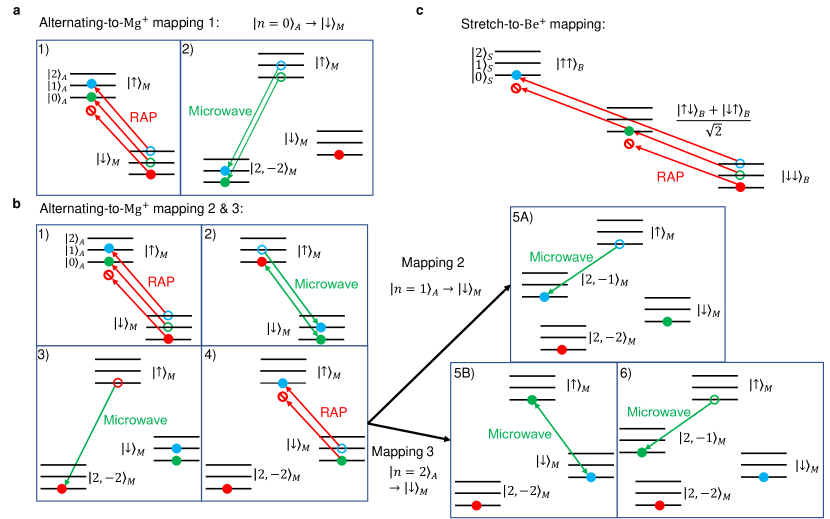
Figure 5: Diagram of motion-to-spin mapping for determining joint populations of motional modes. Circles in different colors represent the initial population in $\left|n=0\right\rangle$ (red), $\left|1\right\rangle$ (green), $\left|2\right\rangle$ (blue) at the beginning of the illustrated step and solid dots at the end. Transitions are indicated by arrows and forbidden transitions are indicated by a prohibitory symbol at the tip of the arrow.

• Alternating-to-Mg⁺ mapping: One of three different mapping sequences (Fig. 5a, b) maps the population in one of the three lowest number states respectively onto the bright state $\left|\downarrow\right\rangle_{M}$ and shelves the other two number states to dark states, $\left|2,-1\right\rangle_{M}$ and $\left|2,-2\right\rangle_{M}$. Repeated experimental trials with different choices of mapping sequences are used to build statistics for the populations of $|0\rangle$, $|1\rangle$, and $|2\rangle$.
  
  The mapping 1 for $\left|0\right\rangle_{A}\rightarrow\left|\downarrow\right\rangle_{M}$ (Fig. 5a) is as follows: 1) A MSS RAP pulse on the $\left|\downarrow\right\rangle_{M}|n\rangle_{A}\rightarrow\left|\uparrow\right\rangle_{M}\left|n-1\right\rangle_{A}$ transition flips the internal state of the Mg⁺ ion from $\left|\downarrow\right\rangle_{M}$ to $\left|\uparrow\right\rangle_{M}$ if the Alternating mode is in $\left|1\right\rangle_{A}$ (green dot) or $\left|2\right\rangle_{A}$ (blue dot) while also subtracting one quantum of motion, but leaves $\left|\downarrow\right\rangle_{M}\left|0\right\rangle_{A}$ (red dot) unchanged. 2) A microwave pulse shelves the population in $\left|\uparrow\right\rangle_{M}$ (the initial population of $\left|1\right\rangle_{A}$ and $\left|2\right\rangle_{A}$) to $\left|2,-2\right\rangle_{M}$.
  
  The mapping 2 for $\left|1\right\rangle_{A}\rightarrow\left|\downarrow\right\rangle_{M}$ and the mapping 3 for $\left|2\right\rangle_{A}\rightarrow\left|\downarrow\right\rangle_{M}$ (Fig. 5b) start similarly. 1) A MSS RAP pulse separates the population of $\left|0\right\rangle_{A}$ from $\left|1\right\rangle_{A}$ and $\left|2\right\rangle_{A}$. 2) Then, a microwave $\pi$ pulse $\left|\uparrow\right\rangle_{M}\leftrightarrow\left|\downarrow\right\rangle_{M}$ is applied. 3) A microwave shelving sequence then transfers the population in $\left|\uparrow\right\rangle_{M}$ (the initial population of $\left|0\right\rangle_{A}$) to $\left|2,-2\right\rangle_{M}$. 4) A second MSS RAP pulse separates the initial population of $\left|1\right\rangle_{A}$ from that of $\left|2\right\rangle_{A}$. 5A) The last step of mapping 2 is to apply a microwave shelving sequence which transfers the initial population of $\left|2\right\rangle_{A}$ (now in $\left|\uparrow\right\rangle_{M}$) to another dark state $\left|2,-1\right\rangle_{M}$ and leaves the initial population of $\left|1\right\rangle_{A}$ still in $\left|\downarrow\right\rangle_{M}$. 5B) For mapping 3, a microwave $\pi$ pulse of $\left|\uparrow\right\rangle_{M}\leftrightarrow\left|\downarrow\right\rangle_{M}$, inserted between the second RAP pulse and the final shelving sequence, maps the population in $\left|2\right\rangle_{A}$ onto $\left|\downarrow\right\rangle_{M}$ instead. 6) The initial population of $\left|1\right\rangle_{A}$ is shelved to $\left|2,-1\right\rangle_{M}$.

• Stretch-to-Be⁺ mapping (Fig. 5c) uses a RAP pulse on the $\left|\downarrow\right\rangle_{B}|n\rangle_{S}\rightarrow\left|\uparrow\right\rangle_{B}\left|n-1\right\rangle_{S}$ transition, flipping both Be⁺ ions from $\left|\downarrow\right\rangle_{B}$ to $\left|\uparrow\right\rangle_{B}$ if $\left|n\right\rangle_{S}=\left|2\right\rangle$, which realizes $\left|\downarrow\downarrow\right\rangle_{B}\left|2\right\rangle_{S}\rightarrow\left|\uparrow\uparrow\right\rangle_{B}\left|0\right\rangle_{S}$; only one ion flips if $\left|n\right\rangle_{S}=\left|1\right\rangle$, $\left|\downarrow\downarrow\right\rangle_{B}\left|1\right\rangle_{S}\rightarrow 1/\sqrt{2}(\left|\uparrow\downarrow\right\rangle_{B}+\left|\downarrow\uparrow\right\rangle_{B})\left|0\right\rangle_{S}$; and the two ions remain in $\left|\downarrow\downarrow\right\rangle_{B}$ when $\left|n\right\rangle_{S}=\left|0\right\rangle$. Before fluorescence detection, the population in $\left|\uparrow\right\rangle_{B}$ of both Be⁺ ions is shelved to the dark state $\left|1,-1\right\rangle_{B}$ (not shown in Fig. 5c).

State-dependent fluorescence detection of Mg⁺ and Be⁺ is performed sequentially after the mapping steps described above to obtain photon counts of both species. We perform three sets of experimental trials with different Alternating-to-Mg⁺ mappings with $N$=1000 trials per set. In each experimental trial, the Be⁺ counts $c_{Be}$ are compared to thresholds $\{$13, 46$\}$ to determine the number of the bright ions $N_{Be}$, which in turn indicates the Stretch mode state based on the mapping

$c_{Be}>$ 46 $\rightarrow N_{Be}$ = 2 $\rightarrow n_{S}$ = 0; 13 $<c_{Be}\leq$ 46 $\rightarrow N_{Be}$ = 1 $\rightarrow n_{S}$ = 1; $c_{Be}\leq$ 13 $\rightarrow N_{Be}$ = 0 $\rightarrow n_{S}$ = 2.

When mapping $\left|n\right\rangle_{A}\rightarrow\left|\downarrow\right\rangle_{M}$, the Alternating mode is declared to be in $\left|n\right\rangle_{A}$ if the Mg⁺ counts are beyond a threshold of nine. Experiments with the Mg⁺ counts below the threshold of nine are discarded because the Alternating mode is likely in one of the other two number states and we cannot distinguish them in such cases. We calculate the populations of the nine joint states $\{|n\rangle_{A}|m\rangle_{S}\}$ ($n,m$ = 0, 1, 2) according to $P_{i}^{(0)}$=$N^{(0)}_{i}/N_{rep}$, ($i$=0,…,9) with $N^{(0)}_{i}$ the occurrence of the $i$-th joint state and $N_{rep}$ the total number of successful repetitions of a certain mapping. The populations are then normalized to their sum using $P_{i}=P_{i}^{(0)}/(\sum_{i=1}^{9}P_{i}^{(0)})$ to yield the final data. Uncertainties are calculated assuming that projection noise is the dominant noise source, $\Delta P_{i}=\sqrt{P_{i}(1-P_{i})/N_{rep}}$.

Experimental results shown in Fig. 2e-j have appreciable state preparation and measurement (SPAM) errors. State preparation errors are from imperfect sideband cooling and imperfect phonon injection, as mentioned above. Measurement errors arise from imperfect mapping operations consisting of RAP pulses ($\sim$5% error per RAP pulse) and microwave pulse sequences. Since the mapping process takes between 2.6 ms and 3.8 ms, heating during mapping can change the motional state, with the Alternating mode being more affected than the Stretch mode. The motional state measurement error from heating varies for different number states and scales approximately with $n_{A}+1/2$ since the Alternating mode heating rate is much higher than that of the Stretch mode. The readout error due to the threshold method is estimated to be negligible. Precise determination of how SPAM errors compound for each joint state is complicated, so we did not attempt this. The error sources discussed here approximately explain the SPAM errors observed in the experiments.

Minimization of Mg⁺ participation in the Stretch mode
Anharmonicity in the external trap potential and higher-order terms (beyond the term linear in ion displacement) of the Taylor expansion of Coulomb force can impact mode participation of a multi-ion string Home et al. (2011). In our experiments, we consider three types of anharmonic terms including the radial gradients $\partial U/\partial x$ and $\partial U/\partial y$, the twist curvature term $\partial^{2}U/(\partial x\partial z)$, and the axial cubic term $\partial^{3}U/\partial z^{3}$. Non-zero values for these terms lead to non-zero participation of the Mg⁺ ion in the Stretch mode, which will then be coupled to recoil from Mg⁺ scattering events. To minimize these terms, we cool the Stretch mode to its ground state and apply “shim” voltages (shims) found based on trap simulations to mimimize relevant anharmonic terms, using a minimal amount of heating of the Stretch mode from Mg⁺ photon scattering as the figure of merit. Radial gradients are controlled by a differential voltage shim on the pair of control electrodes closest to the ions and an additional voltage shim applied to a bias electrode on a third-layer wafer outside the two main wafers Blakestad (2010). The twist term is controlled by the two pairs of electrodes next to the two electrodes closest to the ions. By applying a differential voltage shim of $v$ on the pair of electrodes on one side and $-v$ on the other, the twist of the ion string in the $x-z$ plane relative to the trap axis can be minimized. The cubic term $z^{3}$ is controlled with the same electrodes used for creating the Alternating-Stretch coupling. The optimal shim values are determined as follows: All three axial modes are sideband cooled close to their ground states, then the voltage shim controlling one of the anharmonicity terms is set to a certain strength. Mg⁺ resonant light is pulsed for 1 ms to cause scattering on Mg⁺, then the applied anharmonicity shim is set back to zero and probability of a state change of Be⁺ when driving a MSS pulse is determined. The shim with minimal MSS spin-flip probability is retained as optimal and applied for subsequent experiments. Since the shims are not perfectly decoupled from each other, we iterate the minimization of all three anharmonic terms for several rounds to find the overall best shims. However, we still observe small residual heating of the Stretch mode due to scattering on Mg⁺. This could be because the anharmonicity is still not totally eliminated. Another potential source is radiation pressure on the Mg⁺ ion, which shifts its position relative to the Be⁺ ions slightly during photon scattering and breaks the mirror symmetry of the ion string.

Calibration of the Cirac-Zoller mapping for repeated motional state measurements
In the repeated motional state measurements, a Cirac-Zoller (CZ) sequence maps information about the Alternating mode state onto the Mg⁺ internal state. The basic principle is that a motion-subtracting-sideband 2$\pi$ pulse does not change motional states $|0\rangle$ and $|1\rangle$ but leads to a motional-state-dependent phase shift on the Mg⁺ internal state. The Mg⁺ is prepared in $\left|3,1\right\rangle_{M}$ with optical pumping, followed by a microwave $\pi$ pulse sequence. Then, a microwave carrier $\pi$/2 pulse of $\left|3,1\right\rangle_{M}\leftrightarrow\left|2,0\right\rangle_{M}$ generates a superposition state $1/\sqrt{2}\left(\left|2,0\right\rangle_{M}+\left|3,1\right\rangle_{M}\right)$. Next, the population in $\left|3,1\right\rangle_{M}$ is transferred to $\left|2,2\right\rangle_{M}$ by a microwave $\pi$ pulse followed by a MSS 2$\pi$ pulse of $\left|2,2\right\rangle_{M}\left|1\right\rangle_{A}\leftrightarrow\left|3,3\right\rangle_{M}\left|0\right\rangle_{A}$. For $\left|n=0\right\rangle_{A}$, the MSS pulse does not change the Alternating mode or the Mg⁺ internal state, and the system remains in $1/\sqrt{2}(\left|2,0\right\rangle_{M}+\left|2,2\right\rangle_{M})\left|0\right\rangle_{A}$. For $\left|n=1\right\rangle_{A}$, the MSS pulse drives $\left|2,2\right\rangle_{M}\left|1\right\rangle_{A}$ to $\left|3,3\right\rangle_{M}\left|0\right\rangle_{A}$ and back to $-\left|2,2\right\rangle_{M}\left|1\right\rangle_{A}$, flipping the sign of this component. The state is changed to $1/\sqrt{2}(\left|2,0\right\rangle_{M}-\left|2,2\right\rangle_{M})\left|1\right\rangle_{A}$ in this case. After the MSS pulse, the population in $\left|2,2\right\rangle_{M}$ is transferred back to $\left|3,1\right\rangle_{M}$ with a microwave $\pi$ pulse. Subsequently, a second microwave $\pi$/2 pulse of $\left|3,1\right\rangle_{M}\leftrightarrow\left|2,0\right\rangle_{M}$ with a relative phase $\phi_{2}$ with respect to the first $\pi$/2 pulse is applied. The populations in $\left|3,1\right\rangle_{M}$ and $\left|2,0\right\rangle_{M}$ are shelved to $\left|3,3\right\rangle_{M}$ (the bright state) and $\left|2,-2\right\rangle_{M}$ (the dark state) respectively by a microwave sequence before Mg⁺ fluorescence detection.

The probability of Mg⁺ being measured in bright ($b$) or dark ($d$) is given by $P(b)=(1-\cos(\phi_{2}))/2$ and $P(d)=(1+\cos(\phi_{2}))/2$. By setting $\phi_{2}=0$, $\left|0\right\rangle_{A}$ is mapped to $d$ while $\left|1\right\rangle_{A}$ is mapped to $b$. The mapping $\left|0\right\rangle_{A}\rightarrow b$ and $\left|1\right\rangle_{A}\rightarrow d$ is realized by setting $\phi_{2}=\pi$. The particular transitions chosen in the CZ mapping implementation yield the shortest duration of the sequence in our apparatus, which reduces errors due to heating and dephasing. The phases $\phi_{2}$ are calibrated periodically to account for experimental drifts. We calibrate $\phi_{2}$ with the Alternating mode prepared in $\left|0\right\rangle_{A}$ and $\left|1\right\rangle_{A}$, which yields two out-of-phase sinusoidal signals as a function of $\phi_{2}$, as shown in Fig. 12a; we use the $\phi_{2}$ yielding maximal or minimal fluorescence for realizing the respective mappings. When the Alternating mode contains population in states with $\left|n>1\right\rangle_{A}$, the MSS pulse no longer accomplishes a 2$\pi$ rotation and changes the Alternating mode state. Therefore, this particular measurement does not preserve the motional state if it contains any population outside $\{\left|0\right\rangle_{A},\left|1\right\rangle_{A}\}$.

State verification after repeated motional state measurements
The final state after $N$ motional state measurements is examined with MAS and MSS $\pi$ pulses. In Fig. 12b, with $N=1$ and M1, we detect $\{o_{1}\}=\{d\}$ heralding $\left|0\right\rangle$ with a probability of 0.960(3), close to $p_{0}$ but with a small difference indicating a readout error of about $\epsilon_{0}$ $\approx$ 0.02. The MAS (pink bar) and MSS (violet bar) results conditioned on $\{d\}$ are close to their ideal values (hatched bars) for $\left|0\right\rangle$, suggesting that this conditioned final state is preserved during the measurement and close to $\left|0\right\rangle$. However, the sideband results conditioned on $\{o_{1}\}=\{b\}$ heralding $\left|1\right\rangle$ significantly deviate from their ideal values for $\left|1\right\rangle$. This is because the probability of getting a false outcome for $\left|0\right\rangle$, $p_{0}\epsilon_{0}\approx$ 0.02, is comparable to $p_{1}$, thus causing a noticeable effect on the heralded results for $\left|1\right\rangle$. Erroneous declarations can be reduced by repeating the measurement. When $N=2$, the sideband results conditioned on $\{o_{1},o_{2}\}=\{b,b\}$ are significantly closer to the ideal expectation for $\left|1\right\rangle$ even though Mg⁺ scatters double the amount of photons. When $N=3$, the final states conditioned on $\{o_{1},o_{2},o_{3}\}=\{b,b,b\}$ match the expectation values even more closely. The post-selected results for $\left|0\right\rangle$ also show improved accuracy relative to the MAS/MSS analysis when increasing the number of measurements. We observed similar performance when implementing M2 but with the roles of $\left|0\right\rangle$ and $\left|1\right\rangle$ flipped.

Characterization of heating associated with repeated motional state measurements
We perform a series of tests to characterize the heating from each element in the motional state measurement sequence. All three axial modes are sideband cooled to near their ground states and the Mg⁺ ion is prepared in $\left|\downarrow\right\rangle_{M}$. Then, modified measurement sequences are implemented with different combinations of CZ mapping, swap pulses, Mg⁺ detection, and Mg⁺ sideband cooling of the INPH and Alternating modes. Elements that are not applied are sometimes replaced with a delay of equal duration to account for anomalous heating. This is followed by either applying a Alternating MAS or MSS $\pi$ pulse and determining the respective spin-flip probabilities $P_{\rm MSS}$ and $P_{\rm MAS}$. The ratio of spin-flip probabilities $r=P_{\rm MSS}/P_{\rm MAS}$ is then used to estimate the average motional occupation $\bar{n}=r/(1-r)$ of the Alternating mode. This estimate is accurate if the motional state is well-described by a thermal distribution or if the probability for number states with $n>1$ can be neglected. More details and results of these tests are shown in Table 4.

We measure the mean occupation of the Alternating mode immediately after sideband cooling to be $\bar{n}_{\rm SBC}$ = 0.023(1) as a reference value. In the “no swaps” test, the two swaps are replaced with two delays of equal duration, which yields $\bar{n}$ = 0.040(3), higher than $\bar{n}_{\rm SBC}$ by $\Delta\bar{n}$ = 0.017(3) due to the heating of the Alternating mode acting over the delay replacing the second swap. This test also approximately sets a lower bound for $\bar{n}$ when at least one measurement is performed and no outcome is used for post-selection. Next, we perform the swap test where only two swap pulses are applied after sideband cooling. We find a rise in $\bar{n}$ by $\Delta\bar{n}$ = 0.021(4) from two swaps. In the CZ heating test, a delay of equal duration as a CZ mapping sequence is inserted before swaps and further increases $\bar{n}$ by $\Delta\bar{n}\approx$  0.005. To estimate the $\Delta\bar{n}$ due to heating of the Stretch mode during Mg⁺ detection and SBC of the other two modes, we apply a delay equal to the duration of Mg⁺ detection followed by Mg⁺ sideband cooling and find an increase of $\Delta\bar{n}$ = 0.010(5). In the recoil heating test, we apply Mg⁺ detection to investigate the additional heating of the Stretch mode from recoil of photons scattered on Mg⁺. We estimate $\Delta\bar{n}\approx$   0.012(5) added to $\bar{n}$ from scattered photons alone. An ion typically scatters on the order of a few tens of photons during sideband cooling while on the order of 10³ photons are scattered during fluorescence detection. Assuming recoil heating is proportional to scattered photon number, scattering during sideband cooling only causes a negligible gain in $\bar{n}$ on the order of 10^-4. Lastly, we implement a test (labelled as “No exchange” in Fig. 3d) of the main text) that replaces $N$=1, 2, 3 measurement blocks with an equal delay and obtain $\bar{n}$ = 0.25(3), 0.51(6), 0.8(1), respectively, which are significantly higher than $\bar{n}_{\rm SBC}$, because the motional state resides longer in the Alternating mode at a higher heating rate, compared to $N$ measurement blocks where the mode is swapped to the Stretch mode for substantial parts of the experiments.

Exp.	M1 ($N$ = 1)			M2 ($N$ = 1)
$\{o_{1}\}$	$\{d\}$	$\{b\}$	Overall	$\{d\}$	$\{b\}$	Overall
MAS	0.931(4)	0.76(3)	0.924(3)	0.84(2)	0.915(4)	0.910(4)
MSS	0.030(2)	0.49(3)	0.048(3)	0.33(2)	0.044(3)	0.064(3)
Prob.	0.960(3)	0.040(3)	1	0.066(3)	0.934(3)	1

Table 1: Sideband transition probabilities conditioned on different motional state measurement outcomes for $N$=1. The table shows the probability of a spin flip after a MAS or MSS $\pi$ pulse, conditioned on $\{o_{1}\}$=$\{d\}$ and $\{b\}$ for mapping M1 and M2 and the probability of outcomes $d$ and $b$. The overall sideband spin-flip probabilities with no conditioning on measurement outcomes are also shown.

Exp.	M1 ($N$ = 2)					M2 ($N$ = 2)
$\{o_{1},o_{2}\}$	$\{d,d\}$	$\{d,b\}$	$\{b,d\}$	$\{b,b\}$	Overall	$\{d,d\}$	$\{d,b\}$	$\{b,d\}$	$\{b,b\}$	Overall
MAS	0.924(4)	0.78(2)	0.88(2)	0.57(4)	0.908(4)	0.56(4)	0.91(2)	0.73(2)	0.929(4)	0.903(4)
MSS	0.027(2)	0.46(3)	0.08(2)	0.77(4)	0.066(3)	0.73(4)	0.05(1)	0.53(2)	0.044(3)	0.102(4)
Prob.	0.900(4)	0.049(3)	0.029(2)	0.022(2)	1	0.025(2)	0.042(3)	0.083(4)	0.850(5)	1

Table 2: Sideband transition probabilities conditioned on different motional state measurement outcomes for $N$ = 2. Similar to table 1, listing results for all combinations of two measurement outcomes.

Exp.	M1 ($N$ = 3)
$\{o_{1},o_{2},o_{3}\}$	$\{d,d,d\}$	$\{d,d,b\}$	$\{d,b,d\}$	$\{d,b,b\}$	$\{b,d,d\}$	$\{b,d,b\}$	$\{b,b,d\}$	$\{b,b,b\}$	{Majority $d$}	{Majority $b$}	Overall
MAS	0.935(2)	0.74(2)	0.89(2)	0.64(3)	0.93(2)	0.60(8)	0.75(6)	0.59(4)	0.926(2)	0.63(2)	0.912(3)
MSS	0.025(2)	0.51(2)	0.13(2)	0.78(2)	0.03(1)	0.78(7)	0.22(6)	0.82(3)	0.047(2)	0.74(2)	0.08(2)
Prob.	0.876(6)	0.036(2)	0.020(1)	0.024(1)	0.021(1)	0.0028(5)	0.0046(6)	0.016(1)	0.952(1)	0.048(1)	1
Exp.	M2 ($N$ = 3)
$\{o_{1},o_{2},o_{3}\}$	$\{d,d,d\}$	$\{d,d,b\}$	$\{d,b,d\}$	$\{d,b,b\}$	$\{b,d,d\}$	$\{b,d,b\}$	$\{b,b,d\}$	$\{b,b,b\}$	{Majority $d$}	{Majority $b$}	Overall
MAS	0.48(9)	1.0	0.8(1)	0.92(3)	0.66(5)	0.88(4)	0.72(4)	0.927(7)	0.64(4)	0.908(7)	0.891(7)
MSS	0.80(8)	0.07(7)	0.4(2)	0.03(2)	0.76(5)	0.04(2)	0.46(4)	0.045(5)	0.68(4)	0.077(6)	0.118(7)
Prob.	0.015(3)	0.004(1)	0.006(2)	0.034(4)	0.043(5)	0.042(5)	0.075(6)	0.783(9)	0.067(4)	0.933(4)	1

Table 3: Sideband transition probabilities conditioned on different motional state measurement outcomes for $N$ = 3. Similar to the previous two tables. In addition, majority $d$ or $b$ is conditioned on at least two out of three outcomes being $d$ or $b$.

	CZ mapping	Swaps	Mg detection	Mg SBC	$\bar{n}$	$\Delta\bar{n}$
SBC	No	No	No	No	0.023(1)	0
No-swaps test	Yes	Replaced with delay	Yes	Yes	0.040(3)	0.017(3)
Swap test	No	Yes	No	No	0.044(3)	0.021(4)
CZ heating test	Replaced with delay	Yes	No	No	0.049(4)	0.026(5)
Stretch heating test	Replaced with delay	Yes	Replaced with delay	Yes	0.059(4)	0.036(5)
Recoil heating test	Replaced with delay	Yes	Yes	Yes	0.071(5)	0.048(5)
No exchange ($N=1$)	Replaced with delay	Replaced with delay	Replaced with delay	Replaced with delay	0.25(3)	0.23(3)
No exchange ($N=2$)	Replaced with delay	Replaced with delay	Replaced with delay	Replaced with delay	0.51(6)	0.49(6)
No exchange ($N=3$)	Replaced with delay	Replaced with delay	Replaced with delay	Replaced with delay	0.8(1)	0.8(1)

Table 4: Experiments to characterize heating associated with certain parts of the motional state measurement. A series of tests to delineate heating of different elements of the measurements, including CZ mapping, swaps, Mg detection, and Mg SBC. Each element is either applied (“Yes”), omitted (“No”), or “Replaced with delay” of the same duration as the element in these tests. The Alternating mode $\bar{n}$ of all tests and the relative increase $\Delta\bar{n}=\bar{n}-\bar{n}_{\rm SBC}$ are listed.

Exp.	M1 ($N$ = 1)		M1 ($N$ = 2)
Condition	$\{o_{1}\}$=$\{d\}$	No post-selection	$\{o_{2}\}$=$\{d\}$	$\{o_{1},o_{2}\}$=$\{d,d\}$	No post-selection
$\bar{n}$	0.034(3)	0.055(3)	0.032(3)	0.030(3)	0.078(4)
Exp.	M1 ($N$ = 3)
Condition	$\{o_{3}\}$=$\{d\}$	$\{o_{2},o_{3}\}$=$\{d,d\}$	$\{o_{1},o_{2},o_{3}\}$=$\{d,d,d\}$	{Majority $d$}	No post-selection
$\bar{n}$	0.032(2)	0.028(2)	0.027(2)	0.053(2)	0.095(3)

Table 5: Mean occupations of the Alternating mode conditioned on different motional state measurement outcomes with mapping M1 ($\left|0\right\rangle\rightarrow d$, $\left|1\right\rangle\rightarrow b$).

Exp.	M2 ($N$ = 1)		M2 ($N$ = 2)
Condition	$\{o_{1}\}$=$\{b\}$	No post-selection	$\{o_{2}\}$=$\{b\}$	$\{o_{1},o_{2}\}$=$\{b,b\}$	No post-selection
$\bar{n}$	0.050(3)	0.075(4)	0.049(3)	0.049(3)	0.127(6)
Exp.	M2 ($N$ = 3)
Condition	$\{o_{3}\}$=$\{b\}$	$\{o_{2},o_{3}\}$=$\{b,b\}$	$\{o_{1},o_{2},o_{3}\}$=$\{b,b,b\}$	{Majority $b$}	No post-selection
$\bar{n}$	0.050(6)	0.050(6)	0.050(6)	0.093(8)	0.15(9)

Table 6: Mean occupations of the Alternating mode conditioned on different motional state measurement outcomes with mapping M2 ($\left|0\right\rangle\rightarrow b$ and $\left|1\right\rangle\rightarrow d$).

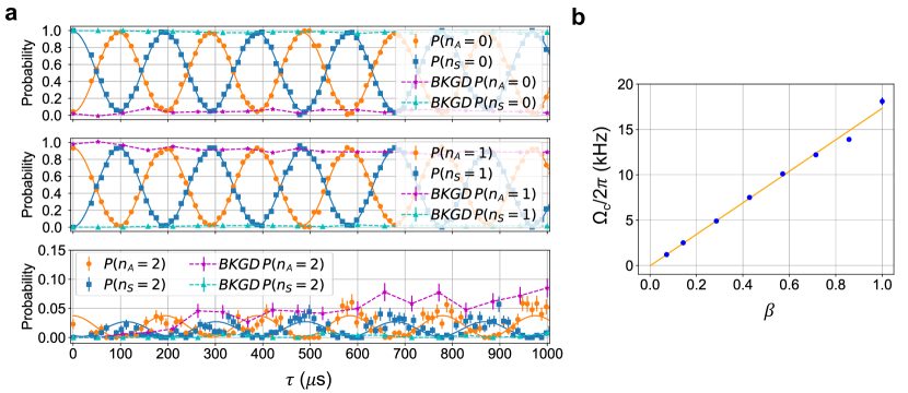
Figure 6: Characterization of the Alternating-Stretch coupling. a, With the Alternating and Stretch mode prepared in $\left|1\right\rangle_{A}\left|0\right\rangle_{S}$, the probabilities of the Alternating (orange dots) and Stretch (blue squares) modes in number state $n$=0 (top), $n$=1 (middle, also partially shown in Fig. 2c), $n$=2 (bottom), oscillate as the coupling pulse duration is varied while the coupling frequency is held on resonance. As references, we repeat the experiment by replacing the coupling pulse with a delay of the same duration to investigate effects of heating, and show the corresponding probabilities of certain number states in the Alternating (magenta stars) and Stretch (cyan triangles) modes in the three panels. The population mostly stays in $n$=0 and $n$=1, while oscillating out of phase between the two modes at $\Omega_{c}=2g_{0}$. In the bottom panel, the populations in $n$=2 of the two modes show small oscillations (due to imperfect state preparation) on top of a slowly growing background that is roughly the average heating rate of the two coupled modes, as independently verified by the reference data (magenta stars and cyan triangles). Solid lines are fits to the data and dashed lines are the guides to the eye. b, The population exchange rate $\Omega_{c}$ can be varied by controlling the amplitude of the coupling potential with a relative factor $0\leq\beta\leq 1$, such that $U(\textbf{r})=\beta U_{max}(\textbf{r})$. This is accomplished by scaling the oscillating potential amplitude of electrode $i$ with $V_{i}=\beta V_{max,i}$ for all twelve electrodes ($i=1,2,...,12$). We choose $\beta$=0.286 for all other results presented in this work. Using higher $\beta$ causes larger unintended excitation of the INPH mode.

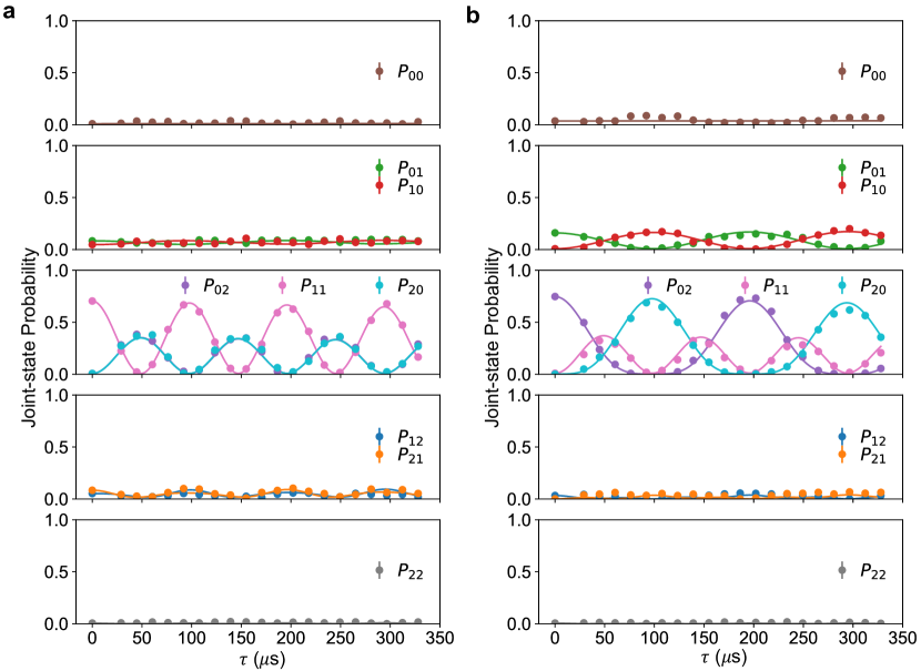
Figure 8: Joint-motional population dynamics: Coupling time scans II. The Alternating and Stretch modes are prepared in (a) $\left|1\right\rangle_{A}\left|1\right\rangle_{S}$ , (b) $\left|0\right\rangle_{A}\left|2\right\rangle_{S}$.

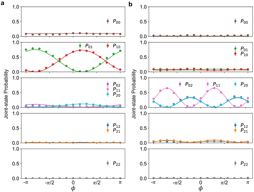
Figure 9: Joint-motional population dynamics: Coupling phase scans. Phonon interference with the initial states (a) $\left|1\right\rangle_{A}\left|0\right\rangle_{S}$ and (b) $\left|1\right\rangle_{A}\left|1\right\rangle_{S}$. The results in the second panel of a and the third panel of b are also shown in Fig. 2i and j of the main text.

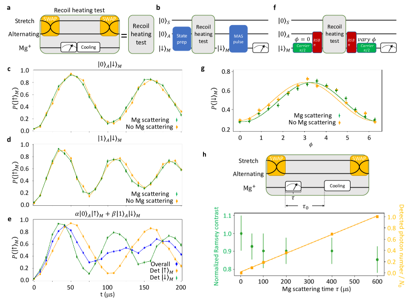
Figure 11: Effects of recoil heating on the protected mode. a, Circuit diagram for Mg⁺ recoil heating test. The test sequence consists of two swap pulses that exchange the states between the Stretch (“protected”) and the Alternating mode, Mg⁺ detection, and a sideband cooling sequence for the INPH mode. Mg⁺ detection can be replaced with a delay of the same duration as required. b, Circuit diagram for testing survival of motional population from Mg⁺ scattering. We prepare the Alternating mode and the Mg⁺ ion in $\left|0\right\rangle_{A}\left|\downarrow\right\rangle_{M}$ (results shown in c), $\left|1\right\rangle_{A}\left|\downarrow\right\rangle_{M}$ (d), and $\alpha\left|0\right\rangle_{A}\left|\uparrow\right\rangle_{M}+\beta\left|1\right\rangle_{A}\left|\downarrow\right\rangle_{M}$ where $|\alpha|^{2}\approx|\beta|^{2}\approx 0.5$ (e), then apply the recoil test sequence with or without Mg⁺ scattering, and finally apply a Alternating MAS pulse with a varying duration followed by Mg⁺ fluorescence detection. In c and d, without (orange squares) and with (green triangles) scattering thousands of photons from the Mg⁺ ion, we obtained nearly identical MAS excitation traces, implying that the motional state is not perturbed substantially by the Mg⁺ ion recoil while stored in the Stretch mode. e, The blue dots are the MAS oscillation results averaged over all experimental trials while disregarding the detection outcome from Mg⁺ in the middle of the experiment, with a rapid decay of contrast due to the mixture of motional states that remains after detection. However, if the MAS results are sorted based on the middle detection outcomes, we obtain two traces for when $\left|\uparrow\right\rangle_{M}$ and $\left|\downarrow\right\rangle_{M}$ are detected that project the motional state onto $\left|0\right\rangle_{A}$ (orange squares) and $\left|1\right\rangle_{A}$ (green triangles) respectively. The sorted trace for $\left|0\right\rangle_{A}$ ($\left|1\right\rangle_{A}$) is nearly identical to the trace in c (d) where $\left|0\right\rangle_{A}$ ($\left|1\right\rangle_{A}$) is directly prepared without a measurement on Mg⁺. The decay of contrast in these oscillation curves is mainly caused by fluctuations in the Rabi-frequency (Debye-Waller effect) due to substantial heating of the in-phase mode. f, Circuit diagram for testing survival of motional coherence between $\left|0\right\rangle_{A}$ and $\left|1\right\rangle_{A}$ during Mg⁺ scattering. A carrier $\pi$/2 pulse of $\left|\downarrow\right\rangle_{M}\leftrightarrow\left|\uparrow\right\rangle_{M}$ with a subsequent red-sideband (RSB) $\pi$ pulse of $\left|\downarrow\right\rangle_{M}\left|1\right\rangle_{A}\leftrightarrow\left|\uparrow\right\rangle_{M}\left|0\right\rangle_{A}$ prepares the Alternating mode in a superposition state $1/\sqrt{2}(\left|0\right\rangle_{A}+\left|1\right\rangle_{A})$ and Mg⁺ in $\left|\downarrow\right\rangle_{M}$. After the recoil heating test sequence, another RSB $\pi$ pulse and carrier $\pi$/2 pulse with varying phase $\phi$ relative to the first $\pi$/2 pulse close the motional Ramsey interferometer. g. The motional Ramsey fringes with (green triangles) or without (orange squares) Mg⁺ scattering have similar contrast which indicates the motional coherence is preserved despite scattering many photons while detecting the internal state of Mg⁺. The imperfect Ramsey contrast of these two curves is likely caused by imperfect preparation, motional dephasing and readout errors. h. With a fixed duration $\tau_{0}$ = 800 $\mu$s between the first swap and recooling of the INPH mode, we vary Mg⁺ scattering time $\tau$. We observe the detected photon number (orange squares, normalized to $N_{0}$ = 51.6) linearly increases over $\tau$ while the motional Ramsey contrast (green dots, normalized to the contrast of 0.41(4) for $\tau$ = 0 $\mu$s) remains unchanged within the experimental uncertainty as more photons are scattered.