Maximizing Global Model Appeal in Federated Learning

Abstract

Federated learning typically considers collaboratively training a global model using local data at edge clients. Clients may have their own individual requirements, such as having a minimal training loss threshold, which they expect to be met by the global model. However, due to client heterogeneity, the global model may not meet each client’s requirements, and only a small subset may find the global model appealing. In this work, we explore the problem of the global model lacking appeal to the clients due to not being able to satisfy local requirements. We propose MaxFL, which aims to maximize the number of clients that find the global model appealing. We show that having a high global model appeal is important to maintain an adequate pool of clients for training, and can directly improve the test accuracy on both seen and unseen clients. We provide convergence guarantees for MaxFL and show that MaxFL achieves a $22$-$40\%$ and $18$-$50\%$ test accuracy improvement for the training clients and unseen clients respectively, compared to a wide range of FL modeling approaches, including those that tackle data heterogeneity, aim to incentivize clients, and learn personalized or fair models.

1 Introduction

Federated learning (FL) is a distributed learning framework that considers training a machine learning model using a network of clients (e.g., mobile phones, hospitals), without directly sharing client data with a central server [1]. FL is typically performed by aggregating clients’ updates over multiple communication rounds to produce a global model [2]. In turn, each client may have its own requirement that it expects to be met by the resulting global model. For example, clients such as hospitals or edge-devices may expect that the global model at least performs better than a local model trained in isolation on the client’s limited local data before contributing to FL training. Unforunately, due to heterogeneity across the clients, the global model may fail to meet all the clients’ requirements [3].

In this work, we say that a global model is appealing to a client if it satisfies the client’s specified requirement, such as incurring at most some max training loss. Subsequently, we define the number of clients which find the global model appealing as global model appeal (formally defined in Definition 1). We find that having a high global model appeal is critical to maintain a large pool of clients to select from for training, and for gathering additional willingly participating clients. This is especially true in the light of clients possibly opting out of FL due to the significant costs associated with training (e.g., computational overhead, privacy risks, logistical challenges). With a larger pool of clients to select from, i.e., with a higher global model appeal, a server can not only improve privacy-utility trade-offs [4], but can also improve the test accuracy of the seen clients, and produce a global model that generalizes better at inference to new unseen clients (see Fig. 1 and Table 1).

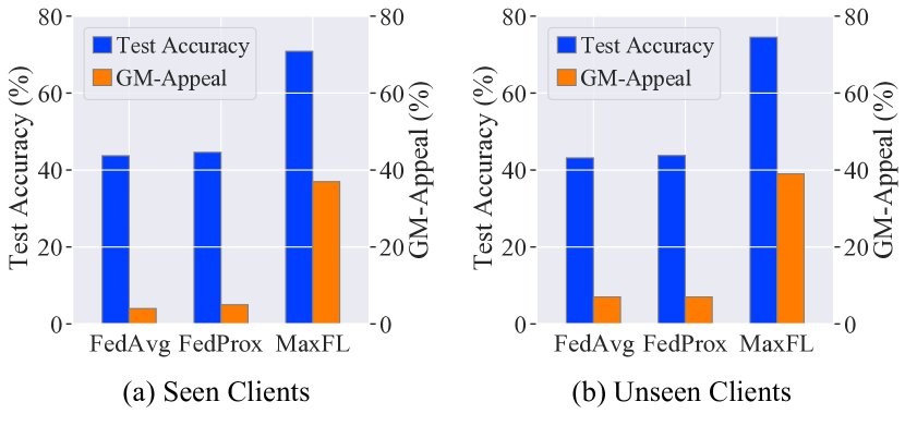
Figure 1: Test accuracy and global model appeal (GM-Appeal) of the global model for FMNIST dataset with the seen clients that have participated during training and unseen clients that have not (more details in Table 1). A higher GM-Appeal results in a higher test accuracy for both types of clients due to the server having a larger pool of clients to select from. MaxFL, which aims to maximize GM-Appeal, results in the highest test accuracy compared to the other baselines that do not consider GM-Appeal.

In this work, we seek to understand: (1) What strategies exist to maximize global model appeal in federated settings, and (2) What benefits exist when maximizing this notion relative to other common federated modeling approaches. Our key contributions are summarized as follows:

• We introduce the notion of global model appeal (referred to as GM-Appeal), which is the fraction of clients that have their local requirements met by the global model.

• We show that having a high global model appeal is imperative for better test accuracy on seen clients as well as better generalization to new unseen clients.

• We propose MaxFL, a novel framework that maximizes global model appeal via a client requirement-aware weighted aggregation of client updates.

• We provide convergence guarantees for our MaxFL solver which allows partial client participation, is applicable to non-convex objectives, and is stateless (does not require clients maintain local parameters during training).

• We empirically validate the performance of MaxFL with experiments where i) clients can flexibly opt-out of training, ii) there are new incoming (unseen) clients, and iii) there are Byzantine clients participating in training.

• We show that MaxFL improves the global model appeal greatly and thus achieves a $22$-$40\%$ and $18$-$50\%$ test accuracy improvement for the seen clients and unseen clients respectively, compared to a wide range of FL methods, including those that tackle data heterogeneity, aim for variance reduction or incentivizing clients, or provide personalization or fairness.

To the best of our knowledge, the notion of global model appeal has not been explored previously in FL. Our work is the first to consider such a notion, show its importance in FL, and then propose an objective to train a global model that can maximize the number of clients whose individual requirements are satisfied. We provide a more detailed review of prior work and related areas of fairness, personalization and client incentives in Section 4.

2 Problem Formulation

We consider a setup where $M$ clients are connected to a central server to collaboratively train a global model. For each client $k\in[M]$, its true loss function is given by $f_{k}(\mathbf{w})=\mathbb{E}_{\xi\sim\mathcal{D}_{k}}[\ell(\mathbf{w},\xi)]$ where $\mathcal{D}_{k}$ is the true data distribution of client $k$, and $\ell(\mathbf{w},\xi)$ is the composite loss function for the model $\mathbf{w}\in\mathbb{R}^{d}$ for data sample $\xi$. In practice, each client only has access to its local training dataset $\mathcal{B}_{k}$ with $|\mathcal{B}_{k}|=N_{k}$ data samples sampled from $\mathcal{D}_{k}$. Client $k$’s empirical loss function is $F_{k}(\mathbf{w})=\frac{1}{|\mathcal{B}_{k}|}\sum_{\xi\in\mathcal{B}_{k}}\ell(\mathbf{w},\xi)$. While some of the take-aways of our work (e.g., improving performance on unseen clients) are more specific to cross-device applications, our general setup and method are applicable to both cross-device and cross-silo FL.

Defining Global Model Appeal. Each client’s natural aim is to find a model that minimizes its true local loss $f_{k}(\mathbf{w})$. Clients can have different thresholds of how small this loss should be, and we denote such self-defined threshold for each client as $\rho_{k},\leavevmode\nobreak\ k\in[M]$. For instance, each client can perform solo training on its local dataset $\mathcal{B}_{k}$ to obtain an approximate local model $\widehat{\mathbf{w}}_{k}$ and have its threshold to be the true loss from this local model, i.e., $\rho_{k}=f_{k}(\widehat{\mathbf{w}}_{k})$. Based on these client requirements, we provide the formal definition of global model appeal below:

Definition 1 (Global Model Appeal).

A global model $\mathbf{w}$ is said to be appealing to client $k\in[M]$ if $f_{k}(\mathbf{w})<\rho_{k}$, i.e., the global model $\mathbf{w}$ yields a smaller local true loss than the self-defined threshold of the client. Global model appeal (GM-appeal) is then defined as the fraction of clients to which the global model is appealing:

$$\textsc{GM-Appeal}=\frac{1}{M}\sum_{k=1}^{M}\mathbb{I}\{f_{k}(\mathbf{w})<\rho_{k}\}$$ (1)

where $\mathbb{I}$ is the indicator function.

Our GM-Appeal metric measures the fraction of clients that find the global model appealing. Note that GM-Appeal only looks at whether the global model satisfies the clients’ requirements or not instead of looking at the gap between $f_{k}(\mathbf{w})$ and $\rho_{k}$. Another variation of 1 could be to measure the margin $\sum_{k}\max\{\rho_{k}-f_{k}(\mathbf{w}),0\}$, but this does not capture the motivation behind our work which is for the server to maximize the number of clients that find the global model appealing. To the best of our knowledge, a similar indicator-based metric has not been explored previously in the FL literature.

2.1 Why GM-Appeal is Important in FL

Before presenting our proposed objective MaxFL that maximizes GM-Appeal, we first elaborate on the significance of the GM-Appeal metric in FL, including how it affects the test performance of the training (seen) clients and the generalization performance on new (unseen) clients at inference.

GM-Appeal measures how many clients’ requirements are satisfied by the global model. Thus, it gauges important characteristics of the global model such as how many clients are likely to dropout with the current global model or how many new incoming clients will likely be satisfied with the current global model. Ultimately, a high global model appeal leads to a larger pool of clients for the server to select from. The standard FL objective [1] does not consider whether the global model satisfies the clients’ requirements, and implicitly assumes that the server will have a large number of clients to select from. However, this may not necessarily be true if clients are allowed to dropout when they find the global model unappealing.

Acquiring a larger pool of clients by improving global model appeal is imperative to improve test accuracy performance of the global model to the seen clients as well as for improving the generalization performance of the global model on the unseen clients at inference (see Fig. 1 and Table 1). In fact, we find that other baselines such as those that aim to tackle data heterogeneity, improve fairness, or provide personalization all have low GM-Appeal, leading to a large number of clients opting out. Due to this, the global model is trained on just a few limited data points, resulting in poor performance. On the other hand, our proposed MaxFL which aims to maximize GM-Appeal is able to retain a large number of clients for training, resulting in a better global model. Moreover, we show that a high GM-appeal for the current set of training (seen) clients also leads to having a high GM-appeal for the unseen clients and also better test accuracy on these new unseen clients at inference.

2.2 Proposed MaxFL Objective

In the previous section, we have shown that having a high global model appeal is imperative to achieve both good test accuracy and generalization performance. In this section, we introduce MaxFL whose aim is to train a global model that maximizes GM-Appeal. A naïve approach is to find the global model that can directly maximize GM-Appeal defined in 1 as follows:

$$\begin{aligned} \operatorname*{argmax}_{\mathbf{w}}\textsc{GM-Appeal}=\operatorname*{argmin}_{\mathbf{w}}\sum_{k=1}^{M}\text{sign}(f_{k}(\mathbf{w})-\rho_{k}).\end{aligned}$$ (2)

where $\text{sign}(x)=1$ if $x\geq 0$ and $0$ otherwise. There are two immediate difficulties in minimizing 2. First, clients may not know their true data distribution $\mathcal{D}_{k}$ to compute $f_{k}(\mathbf{w})-\rho_{k}$. Second, the sign function makes the objective nondifferentiable and limits the use of common gradient-based methods. We resolve these issues by proposing a "proxy" for 2 with the following relaxations.

Replacing the Sign function with the Sigmoid function $\sigma(\cdot)$: Replacing the non-differentiable 0-1 loss with a smooth differentiable loss is a standard tool used in optimization [5, 6]. Given the many candidates (e.g. hinge loss, ReLU, sigmoid), we find that using the sigmoid function is essential for our objective to faithfully approximate the true objective in 2. We discuss the theoretical implications of using the sigmoid loss in more detail in Section A.1.

Replacing $\sigma(f_{k}(\mathbf{w})-\rho_{k})$ with $\sigma(F_{k}(\mathbf{w})-\rho_{k})$: As clients do not have access to their true distribution $\mathcal{D}_{k}$ to compute $f_{k}(\cdot)$ we propose to use an empirical estimate $\sigma(F_{k}(\mathbf{w})-\rho_{k})$. This is again similar to what is done in standard FL where we minimize $F_{k}(\mathbf{w})$ instead of $f_{k}(\mathbf{w})$ at client $k$. Note that the global model $\mathbf{w}$ is trained on the data of all clients, making it unlikely to overfit to the local data of any particular client, leading to $f_{k}(\mathbf{w})\approx F_{k}(\mathbf{w})$, also shown empirically in Section D.2.

With the Sigmoid relaxation, we present our proposed MaxFL objective:

$$\begin{aligned} \text{{MaxFL} Obj.:}\leavevmode\nobreak\ \min_{\mathbf{w}}\widetilde{F}(\mathbf{w})=\min_{\mathbf{w}}\frac{1}{M}\sum_{i=1}^{M}\widetilde{F}_{i}(\mathbf{w}),\leavevmode\nobreak\ \text{where}\leavevmode\nobreak\ \widetilde{F}_{i}(\mathbf{w})\vcentcolon=\sigma(F_{i}(\mathbf{w})-\rho_{i}).\end{aligned}$$ (3)

Our empirical results in Section 5 support our intuition of these relaxations and demonstrate that minimizing our proposed objective leads to a higher GM-Appeal than the standard FL objective. We also provide a theoretical analysis in Section A.1 to illustrate how our MaxFL objective behaves differently from the standard FL objective to maximize global model appeal for mean estimation.

3 Proposed MaxFL Solver

In this section, we present our MaxFL objective’s solver. The MaxFL algorithm enjoys the following properties, which make it a good candidate for real-world applications of cross-device FL: i) uses the same local SGD procedure as in standard FedAvg, ii) allows partial client participation, and iii) is stateless. By stateless, we mean that clients do not carry varying local parameters throughout training rounds, preventing issues from stale parameters [7].

With the sigmoid approximation of sign loss and for differentiable $F_{k}(\mathbf{w})$, our objective $\widetilde{F}(\mathbf{w})$ in 3 is differentiable and can be minimized with gradient descent and its variants. Its gradient is given by:

$$\nabla\widetilde{F}(\mathbf{w})=\frac{1}{M}\sum_{k=1}^{M}\underbrace{(1-\widetilde{F}_{k}(\mathbf{w}))\widetilde{F}_{k}(\mathbf{w})}_{\text{aggregating weight}\vcentcolon=q_{k}(\mathbf{w})}\nabla F_{k}(\mathbf{w}).$$ (4)

Observe that $\nabla\widetilde{F}(\mathbf{w})$ is a weighted aggregate of the gradients of the clients’ empirical losses, similar in spirit to the gradient $\nabla F(\mathbf{w})$ in standard FL. The key difference is that in MaxFL, the weights $q_{k}(\mathbf{w})\vcentcolon=(1-\widetilde{F}_{k}(\mathbf{w}))\widetilde{F}_{k}(\mathbf{w})$ depend on how much the global model appeals to the clients and are dynamically updated based on the current model ${\bf w}$, as we discuss below.

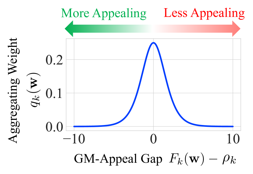
Figure 2: Aggregating weight $q_{k}(\mathbf{w})$ for any client $k$ versus the GM-Appeal gap $F_{k}(\mathbf{w})-\rho_{k}$. The weight is the highest for the clients which the global model performs similarly to the clients’ requirements since this allows it to increase GM-Appeal without sacrificing other clients’ requirements.

Behavior of the Aggregation Weights $q_{k}(\mathbf{w})$. For a given $\mathbf{w}$, the aggregation weights $q_{k}(\mathbf{w})$ depend on the GM-Appeal Gap, $F_{k}(\mathbf{w})-\rho_{k}$ (see Fig. 2). When $F_{k}(\mathbf{w})\ll\rho_{k}$, the global model $\mathbf{w}$ sufficiently meets the client’s requirement. Therefore, MaxFL sets $q_{k}(\mathbf{w})\approx 0$ to focus on the updates of other clients. Similarly, if $F_{k}(\mathbf{w})\gg\rho_{k}$, MaxFL sets $q_{k}(\mathbf{w})\approx 0$. This is because $F_{k}(\mathbf{w})\gg\rho_{k}$ implies that the current model $\mathbf{w}$ is incompatible with the requirement of client $k$ and hence it is better to avoid optimizing for this client at the risk of sacrificing other clients’ requirements. MaxFL gives the highest weight to clients for which the global model performs similarly to the clients’ requirements since this allows it to increase the GM-Appeal without sabotaging other clients’ requirements.

A Practical MaxFL Solver. Directly minimizing the MaxFL objective using gradient descent can be slow to converge and impractical, as it requires all clients to be available for training. Instead, we propose a practical MaxFL algorithm, which uses multiple local updates at each client to speed up convergence as done in standard FL [1] and allow partial client availability.

We use the superscript $(t,r)$ to denote the communication round $t$ and the local iteration index $r$. In each round $t$, the server selects a new set of clients $\mathcal{S}^{(t,0)}$ uniformly at random and sends the most recent global model $\mathbf{w}^{(t,0)}$ to the clients in $\mathcal{S}^{(t,0)}$. Clients in $\mathcal{S}^{(t,0)}$ perform $\tau$ local iterations with a learning rate $\eta_{l}$ to calculate their updates as follows:

$$\mathbf{w}_{k}^{(t,r+1)}=\mathbf{w}_{k}^{(t,r)}-\eta_{l}\mathbf{g}(\mathbf{w}_{k}^{(t,r)},\xi_{k}^{(t,r)}),\forall\leavevmode\nobreak\ r\in\{0,...,\tau-1\}$$ (5)

where $\mathbf{g}(\mathbf{w}_{k}^{(t,r)},\xi_{k}^{(t,r)})=\frac{1}{b}\sum_{\xi\in\xi_{k}^{(t,r)}}\nabla f(\mathbf{w}_{k}^{(t,r)},\xi)$ is the stochastic gradient computed using a mini-batch $\xi_{k}^{(t,r)}$ of size $b$ that is randomly sampled from client $k$’s local dataset $\mathcal{B}_{k}$. The weight $q_{k}(\mathbf{w}_{k}^{(t,0)})$ can be computed at each client by calculating the loss over its training data with $\mathbf{w}_{k}^{(t,0)}$, which is a simple inference step. Clients in $\mathcal{S}^{(t,0)}$ then send their local updates $\Delta\mathbf{w}_{k}^{(t,0)}\vcentcolon=\mathbf{w}_{k}^{(t,\tau)}-\mathbf{w}_{k}^{(t,0)}$ and weights $q_{k}(\mathbf{w}_{k}^{(t,0)})$ back to the server, which updates the global model as follows:

$$\begin{aligned} \mathbf{w}^{(t+1,0)}=\mathbf{w}^{(t,0)}-\eta^{(t,0)}_{g}\sum_{k\in\mathcal{S}^{(t,0)}}q_{k}(\mathbf{w}^{(t,0)})\Delta\mathbf{w}_{k}^{(t,0)}\end{aligned}$$ (6)

where $\eta^{(t,0)}_{g}=\frac{\eta_{g}}{\sum_{k\in\mathcal{S}^{(t,0)}}q_{k}(\mathbf{w}^{(t,0)})+\epsilon}$ is the adaptive server learning rate with global learning rate $\eta_{g}$ and $\epsilon>0$. We discuss the reasoning for such a learning rate below.

Algorithm 1 Our Proposed MaxFL Solver

1:  Input: mini-batch size $b$, local iteration steps $\tau$, client requirement $\rho_{k},\leavevmode\nobreak\ k\in[M]$

2:  Output: Global model $\mathbf{w}^{(T,0)}$

3:  Initialize: Global model $\mathbf{w}^{(0,0)}$

4:  For ${t=0,...,T-1}$ communication rounds do:

5:      Global server do:

6:         Select $m$ clients for $\mathcal{S}^{(t,0)}$ uniformly at random and send $\mathbf{w}^{(t,0)}$ to clients in $\mathcal{S}^{(t,0)}$

7:      Clients $k\in\mathcal{S}^{(t,0)}$ in parallel do:

8:         Set $\mathbf{w}_{k}^{(t,0)}=\mathbf{w}^{(t,0)}$, and calculate $q_{k}(\mathbf{w}_{k}^{(t,0)})=\sigma(F_{k}(\mathbf{w}_{k}^{(t,0)})-\rho_{k})$

9:         For $r=0,...,\tau-1$ local iterations do:

10:           Update $\mathbf{w}_{k}^{(t,r+1)}\leftarrow\mathbf{w}_{k}^{(t,r)}-\eta_{l}\mathbf{g}(\mathbf{w}_{k}^{(t,r)},\xi_{k}^{(t,r)})$

11:         Send $\Delta\mathbf{w}_{k}^{(t,0)}=\mathbf{w}_{k}^{(t,0)}-\mathbf{w}_{k}^{(t,\tau)}$ and aggregation weight $q_{k}(\mathbf{w}_{k}^{(t,0)})$ to the server

12:      Global server do:

13:         Update global model with $\mathbf{w}^{(t+1,0)}=\mathbf{w}^{(t,0)}-\eta^{(t,0)}_{g}\sum_{k\in\mathcal{S}^{(t,0)}}q_{k}(\mathbf{w}^{(t,0)})\Delta\mathbf{w}_{k}^{(t,0)}$

Adaptive Server Learning Rate for MaxFL. With $L_{c}$ continuous and $L_{s}$ smooth $F_{k}(\mathbf{w}),\leavevmode\nobreak\ \forall k\in[M]$ (see 3.1), the objective $\widetilde{F}(\mathbf{w})$ is $\widetilde{L}_{s}$ smooth where $\widetilde{L}_{s}=\frac{L_{s}}{M}\sum_{k=1}^{M}q_{k}(\mathbf{w})+\frac{L_{c}}{4}$ (see Appendix B). Hence, the optimal learning rate $\tilde{\eta}$ for the MaxFL is given by, $\widetilde{\eta}=1/\widetilde{L}_{s}=M\eta/\left({\sum_{k=1}^{M}q_{k}(\mathbf{w})+\epsilon}\right)$, where $\eta=\frac{1}{L_{s}}$ is the optimal learning rate for standard FL and $\epsilon=\frac{ML_{c}}{4L_{s}}$ > 0 is a constant. The denominator of the optimal $\widetilde{\eta}$ is proportional to the sum of the aggregation weights $q_{k}(\mathbf{w})$ and acts as a dynamic normalizing factor. Therefore, we propose using an adaptive global learning rate $\eta^{(t,0)}_{g}=\eta_{g}/(\sum_{k\in\mathcal{S}^{(t,0)}}q_{k}(\mathbf{w}^{(t,0)})+\epsilon)$ with hyperparameters $\eta_{g}$, $\epsilon$.

Example of $\rho_{k}$ as $F_{k}(\widehat{\mathbf{w}}_{k})$ for MaxFL. One intuitive way to set $\rho_{k}$ for each client is to set it as the training loss value $F_{k}(\widehat{\mathbf{w}}_{k})$ where $\widehat{\mathbf{w}}_{k}$ is a client local model that is solo-trained with a few warm-up local SGD steps on its local data. The loss value only needs to be computed once and saved as a constant beforehand at each client. The number of steps for training $\widehat{\mathbf{w}}_{k}$ can be entirely dependent on the personal resources and requirements of the clients. For our experiments, we use the same number of warm-up SGD steps (100 iterations) to achieve the local model $\widehat{\mathbf{w}}_{k}$ across all algorithms and set $\rho_{k}=F_{k}(\widehat{\mathbf{w}}_{k})$ for all our experiments. This gives us a reasonable requirement for each client which is the realistic estimate of the local model accuracy at a client without assuming any significant computation burden at clients. We have also included an ablation study on the effect of the number of local steps to obtain $\widehat{\mathbf{w}}_{k}$ in Section D.2.

Appeal-based Flexible Client Participation. It may appear that our MaxFL solver in Algorithm 1 requires clients to always participate in FL if selected even when the global model does not appeal to them. However, our algorithm can be easily modified to allow clients to participate flexibly during training depending on whether they find the global model appealing or not. For such appeal-based flexible client participation, we assume that clients are available for training if selected only during a few initial training rounds. After these rounds, clients may participate only if they find the global model appealing. We demonstrate this extension of MaxFL with appeal-based flexible client participation in Table 1 and Table 2. These experiments show that with flexible client participation, retaining a high global model is even more imperative for the server to achieve good test accuracy and generalization performance. We also show that even after we allow clients to participate flexibly, MaxFL retains a significantly higher number of clients that find the global model appealing compared to the other baselines.

3.1 Convergence Properties of MaxFL

In this section we show the convergence guarantees of MaxFL in Algorithm 1. Our convergence analysis shows that the gradient norm of our global model goes to zero, and therefore we converge to a stationary point of our objective $\widetilde{F}(\mathbf{w})$. First, we introduce the assumptions and definitions utilized for our convergence analysis below.

Assumption 3.1 (Continuity & Smoothness of $F_{k}(\mathbf{w}),\leavevmode\nobreak\ \forall\leavevmode\nobreak\ k$).

The local objective functions $F_{1}(\mathbf{w}),\leavevmode\nobreak\ ...,F_{M}(\mathbf{w})$, are $L_{c}$-continuous and $L_{s}$-smooth for any $\mathbf{w}$.

Assumption 3.2 (Unbiased Stochastic Gradient with Bounded Variance for $F_{k}(\mathbf{w}),\leavevmode\nobreak\ \forall\leavevmode\nobreak\ k$).

For the mini-batch $\xi_{k}$ uniformly sampled at random from $\mathcal{B}_{k}$, the resulting stochastic gradient is unbiased, i.e., $\mathbb{E}[\mathbf{g}_{k}(\mathbf{w}_{k},\xi_{k})]=\nabla F_{k}(\mathbf{w}_{k})$. The variance of stochastic gradients is bounded: $\mathbb{E}[\|\mathbf{g}_{k}(\mathbf{w}_{k},\xi_{k})-\nabla F_{k}(\mathbf{w}_{k})\|^{2}]\leq\sigma_{g}^{2}$ for $k\in[M]$.

Assumption 3.3 (Bounded Dissimilarity of $F(\mathbf{w})$).

There exists $\beta^{2}\geq 1,\leavevmode\nobreak\ \kappa^{2}\geq 0$ such that $\frac{1}{M}\sum_{i=1}^{M}\|\nabla F_{i}(\mathbf{w})\|^{2}\leq\beta^{2}\|\frac{1}{M}\sum_{i=1}^{M}\nabla F_{i}(\mathbf{w})\|^{2}+\kappa^{2}$ for any $\mathbf{w}$.

3.1-3.3 are standard assumptions used in the optimization literature [8, 9, 10, 11], including the $L_{c}$-continuity assumption [12, 13]. Note that we do not assume anything for our proposed objective function $\widetilde{F}(\mathbf{w})$ and only have assumptions over the standard objective function $F(\mathbf{w})$ to prove the convergence of MaxFL over $\widetilde{F}(\mathbf{w})$ in Theorem 3.1.

Theorem 3.1 (Convergence to the MaxFL Objective $\widetilde{F}(\mathbf{w})$).

Under 3.1-3.3, suppose the server uniformly selects $m$ out of $M$ clients without replacement in each round of Algorithm 1. With $\eta_{l}=\frac{1}{\sqrt{T}\tau},\leavevmode\nobreak\ \eta_{g}=\sqrt{\tau m}$, for a sufficiently large $T$ we have:

$$\begin{aligned} \min_{t\in[T]}\mathbb{E}\left[\left\|\nabla\widetilde{F}(\mathbf{w}^{(t,0)})\right\|^{2}\right]\leq\mathcal{O}\left(\frac{\sigma_{g}^{2}}{\sqrt{m\tau T}}\right)+\mathcal{O}\left(\frac{\sigma_{g}^{2}}{T\tau}\right)+\mathcal{O}\left(\frac{\sqrt{\tau}}{\sqrt{Tm}}\right)+\mathcal{O}\left(\frac{\kappa^{2}+\beta^{2}}{T}\right)\end{aligned}$$ (7)

where $\mathcal{O}$ subsumes all constants (including $L_{s}$ and $L_{c}$).

Theorem 3.1 shows that with a sufficiently large number of communication rounds $T$ we reach a stationary point of our objective function $\widetilde{F}(\mathbf{w})$. The proof is deferred to Appendix B where we also show a version of this theorem that contains the learning rates $\eta_{g}$ and $\eta_{l}$ with the constants.

4 Related Work

To the best of our knowledge, the notion of GM-Appeal and the proposal to maximize it while considering flexible client participation have not appeared before in the previous literature. Previous works have focused on the notion of satisfying clients’ personal requirements from a game-theoretic lens or designing strategies specifically to prevent client dropout, including the use of personalization, which have their limitations, as we discuss below.

4.1 Incentivizing Clients and Preventing drop-out

A recent line of work in game theory models FL as a coalition of self-interested agents and studies how clients can optimally satisfy their individual incentives defined differently from our goal. Instead of training a single global model, [14, 15] consider the problem where each client tries to find the best possible coalition of clients to federate with to minimize its own error. [16] consider an orthogonal setting where each client aims to satisfy its constraint of low expected error while simultaneously trying to minimize the number of samples it contributes to FL. While these works establish useful insights for simple linear tasks, it is difficult to extend these to practical non-convex machine learning tasks. In contrast to these works, in MaxFL we aim to directly maximize the number of satisfied clients using a global model. This perspective alleviates some of the analysis complexities occurring in game-theoretic formulations and allows us to consider general non-convex objective functions.

A separate line of work looks at how to prevent and deal with client drop-out in FL. [17] introduce a notion of ‘friendship’ among clients and proposes to use friends’ local update as a substitute for the update of dropped-out clients. [18] propose to use previous updates of dropped-out clients as a substitute for their current updates. Both algorithms are stateful. Another line of work [19, 20, 21] aims to incentivize clients to contribute resources for FL and promote long-term participation by providing monetary compensation for their contributions, determined using game-theoretic tools. These techniques are orthogonal to MaxFL’s formulation and can be combined if needed to further incentivize clients.

4.2 Personalized and Fair Federated Learning

Personalized federated learning (PFL) methods are able to increase performance by training multiple related models across the network [e.g., 22]. In contrast to PFL, MaxFL focuses on the more challenging goal of training a single global model that can maximize the number of clients for which the global model outperforms their local model. This is because, unlike PFL which may require additional training on new clients for personalization, MaxFL’s global model can be used by new clients without additional training (see Fig. 4). Also, MaxFL is stateless, in that clients do not carry varying local parameters throughout training rounds as in many popular personalized FL methods [22, 23, 24, 25], preventing parameter staleness problems which can be exacerbated by partial client participation [7]. Furthermore, MaxFL is orthogonal to and can be combined with PFL methods. We demonstrate this in Table 3, where we show results for MaxFL jointly used with personalization via fine-tuning [26]. We compare MaxFL $+$Fine-tuning with another well known PFL method PerFedAvg [24] and show that MaxFL appeals to a significantly higher number of clients than the baseline.

Finally, another related area is fair FL, where a common goal is to train a global model whose accuracy has less variance across the client population than standard FedAvg [27, 28]. A side benefit of these methods is that they can improve global model appeal for the worst performing clients. However, the downside is that the performance of the global model may be degraded for the best performing clients, thus making it unappealing for them to participate. We show in Section D.2 that fair FL methods are indeed not effective in increasing GM-Appeal.

	Seen Clients				Unseen Clients
	FMNIST		EMNIST		FMNIST		EMNIST
	Test Acc.	GM-Appeal	Test Acc.	GM-Appeal	Test Acc.	GM-Appeal	Test Acc.	GM-Appeal
FedAvg	$43.70{\scriptstyle(\pm 0.02)}$	$0.04{\scriptstyle(\pm 0.0)}$	$35.15{\scriptstyle(\pm 0.51)}$	$0.02{\scriptstyle(\pm 0.01)}$	$43.14{\scriptstyle(\pm 0.23)}$	$0.07{\scriptstyle(\pm 0.01)}$	$37.14{\scriptstyle(\pm 0.10)}$	$0.06{\scriptstyle(\pm 0.0)}$
FedProx	$44.59{\scriptstyle(\pm 1.94)}$	$0.05{\scriptstyle(\pm 0.01)}$	$34.06{\scriptstyle(\pm 1.21)}$	$0.004{\scriptstyle(\pm 0.0)}$	$43.80{\scriptstyle(\pm 1.67)}$	$0.07{\scriptstyle(\pm 0.01)}$	$36.82{\scriptstyle(\pm 0.22)}$	$0.008{\scriptstyle(\pm 0.0)}$
Scaffold	$39.90{\scriptstyle(\pm 0.59)}$	$0.0{\scriptstyle(\pm 0.0)}$	$34.78{\scriptstyle(\pm 2.05)}$	$0.0{\scriptstyle(\pm 0.0)}$	$39.24{\scriptstyle(\pm 0.68)}$	$0.01{\scriptstyle(\pm 0.0)}$	$34.19{\scriptstyle(\pm 1.25)}$	$0.004{\scriptstyle(\pm 0.0)}$
PerFedAvg	$46.62{\scriptstyle(\pm 1.0)}$	$0.05{\scriptstyle(\pm 0.0)}$	$34.78{\scriptstyle(\pm 1.05)}$	$0.003{\scriptstyle(\pm 0.0)}$	$46.00{\scriptstyle(\pm 0.87)}$	$0.07{\scriptstyle(\pm 0.0)}$	$36.92{\scriptstyle(\pm 0.51)}$	$0.008{\scriptstyle(\pm 0.0)}$
qFFL	$29.92{\scriptstyle(\pm 3.13)}$	$0.0{\scriptstyle(\pm 0.0)}$	$15.95{\scriptstyle(\pm 3.02)}$	$0.0{\scriptstyle(\pm 0.0)}$	$19.63{\scriptstyle(\pm 2.17)}$	$0.0{\scriptstyle(\pm 0.0)}$	$5.41{\scriptstyle(\pm 0.52)}$	$0.0{\scriptstyle(\pm 0.0)}$
MW-Fed	$44.41{\scriptstyle(\pm 2.38)}$	$0.04{\scriptstyle(\pm 0.0)}$	$30.44{\scriptstyle(\pm 3.07)}$	$0.01{\scriptstyle(\pm 0.0)}$	$43.46{\scriptstyle(\pm 2.15)}$	$0.06{\scriptstyle(\pm 0.0)}$	$36.54{\scriptstyle(\pm 0.40)}$	$0.01{\scriptstyle(\pm 0.0)}$
MaxFL	$\mathbf{70.86}{\scriptstyle(\pm 2.18)}$	$\mathbf{0.37}{\scriptstyle(\pm 0.05)}$	$\mathbf{57.34}{\scriptstyle(\pm 1.41)}$	$\mathbf{0.25}{\scriptstyle(\pm 0.03)}$	$\mathbf{74.53{\scriptstyle(\pm 0.50)}}$	$\mathbf{0.39{\scriptstyle(\pm 0.07)}}$	$\mathbf{55.62}{\scriptstyle(\pm 0.86)}$	$\mathbf{0.31}{\scriptstyle(\pm 0.03)}$

Table 1: Avg. test accuracy and GM-Appeal where we train for 200 communication rounds. At the 10th communication round, we let clients flexibly opt-out or opt-in depending on whether the global model has met their requirements. We report the final avg. test accuracy and GM-Appeal at the 200th communication round.

5 Experiments

Datasets and Model.

We evaluate MaxFL in three different settings: image classification for non-iid partitioned (i) FMNIST [29], (ii) EMNIST with 62 labels [30], and (iii) sentiment analysis for (iv) Sent140 [31]with a MLP. For FMNIST, EMNIST, and Sent140 dataset, we consider 100, 500, and 308 clients in total that are used for training where we select 5 and 10 clients uniformly at random per round for FMNIST and EMNIST, Sent140 respectively. These clients are active at some point in training the global model and we call them ‘seen clients’. We also sample the ‘unseen clients’ from the same distribution from which we generate the seen clients, with 619 clients for Sent140, 100 clients for FMNIST, and 500 for EMNIST. These unseen clients represent new incoming clients that have not been seen before during the training rounds of FL to evaluate the generalization performance at inference. Further details of the experimental settings are deferred to Section D.1.

Baselines.

We compare MaxFL with numerous well-known FL algorithms such as standard FedAvg [1]; FedProx [32] which aims to tackle data heterogeneity; SCAFFOLD [9] which aims for variance-reduction; PerFedAvg [24] which facilitates personalization; MW-Fed [16] which incentivizes client participation; and qFFL which facilitates fairness [27]. For all algorithms, we set $\rho_{k}$ to be the same, i.e., $\rho_{k}=F_{k}(\widehat{\mathbf{w}}_{k})$, where $\widehat{\mathbf{w}}_{k}$ is obtained by running a few warm-up local SGD steps on client $k$’s data as outlined in algorithm 1. We do this to ensure a fair comparison across baselines. We perform grid search for hyperparameter tuning for all different baselines and choose the best performing ones.

	Seen Clients
	FMNIST				EMNIST
	Byz=0.1		Byz=0.05		Byz=0.1		Byz=0.05
	Test Acc.	GM-Appeal	Test Acc.	GM-Appeal	Test Acc.	GM-Appeal	Test Acc.	GM-Appeal
MW-Fed	$17.24\leavevmode\nobreak\ {\scriptstyle(\pm 2.35)}$	$0.01\leavevmode\nobreak\ {\scriptstyle(\pm 0.0)}$	$21.28\leavevmode\nobreak\ {\scriptstyle(\pm 1.79)}$	$0.02\leavevmode\nobreak\ {\scriptstyle(\pm 0.0)}$	$15.83\leavevmode\nobreak\ {\scriptstyle(\pm 1.52)}$	$0.004\leavevmode\nobreak\ {\scriptstyle(\pm 0.0)}$	$22.22\leavevmode\nobreak\ {\scriptstyle(\pm 0.63)}$	$0.008\leavevmode\nobreak\ {\scriptstyle(\pm 0.001)}$
MaxFL	$\mathbf{69.42}\leavevmode\nobreak\ {\scriptstyle(\pm 2.87)}$	$\mathbf{0.35}\leavevmode\nobreak\ {\scriptstyle(\pm 0.05)}$	$\mathbf{70.60}\leavevmode\nobreak\ {\scriptstyle(\pm 2.76)}$	$\mathbf{0.42}\leavevmode\nobreak\ {\scriptstyle(\pm 0.03)}$	$\mathbf{52.74}\leavevmode\nobreak\ {\scriptstyle(\pm 0.44)}$	$\mathbf{0.20}\leavevmode\nobreak\ {\scriptstyle(\pm 0.01)}$	$\mathbf{56.10}\leavevmode\nobreak\ {\scriptstyle(\pm 0.77)}$	$\mathbf{0.23}\leavevmode\nobreak\ {\scriptstyle(\pm 0.01)}$
	Unseen Clients
	FMNIST				EMNIST
	Byz=0.1		Byz=0.05		Byz=0.1		Byz=0.05
	Test Acc.	GM-Appeal	Test Acc.	GM-Appeal	Test Acc.	GM-Appeal	Test Acc.	GM-Appeal
MW-Fed	$18.45\leavevmode\nobreak\ {\scriptstyle(\pm 2.81)}$	$0.01\leavevmode\nobreak\ {\scriptstyle(\pm 0.0)}$	$21.91\leavevmode\nobreak\ {\scriptstyle(\pm 3.81)}$	$0.01\leavevmode\nobreak\ {\scriptstyle(\pm 0.0)}$	$17.03\leavevmode\nobreak\ {\scriptstyle(\pm 0.21)}$	$0.005\leavevmode\nobreak\ {\scriptstyle(\pm 0.0)}$	$22.23\leavevmode\nobreak\ {\scriptstyle(\pm 0.63)}$	$0.003\leavevmode\nobreak\ {\scriptstyle(\pm 0.0)}$
MaxFL	$\mathbf{69.75}\leavevmode\nobreak\ {\scriptstyle(\pm 3.66)}$	$\mathbf{0.39}\leavevmode\nobreak\ {\scriptstyle(\pm 0.01)}$	$\mathbf{71.11}\leavevmode\nobreak\ {\scriptstyle(\pm 1.47)}$	$\mathbf{0.46}\leavevmode\nobreak\ {\scriptstyle(\pm 0.01)}$	$\mathbf{53.82}\leavevmode\nobreak\ {\scriptstyle(\pm 0.09)}$	$\mathbf{0.26}\leavevmode\nobreak\ {\scriptstyle(\pm 0.02)}$	$\mathbf{55.10}\leavevmode\nobreak\ {\scriptstyle(\pm 0.78)}$	$\mathbf{0.28}\leavevmode\nobreak\ {\scriptstyle(\pm 0.01)}$

Table 2: Byzantine clients are included in the total clients where they artificially report large losses to the server and add noise to their gradients. The percentage of the Byzantine clients are denoted as ‘Byz’. We report the final avg. test accuracy and GM-Appeal across clients where we train for 200 communication rounds. At the 10th communication round, we let clients flexibly opt-out or opt-in depending on whether the global model has met their requirements.

Evaluation Metrics: GM-Appeal, Average Test Accuracy, and Preferred-model Test Accuracy.

We evaluate MaxFL and other methods with three key metrics: 1) GM-Appeal, defined in (1), 2) average test accuracy (avg. test acc.) across clients, and a new metric that we propose called 3) preferred-model test accuracy. Preferred-model test accuracy is the average of the clients’ test accuracies computed on either the global model $\mathbf{w}$ or their solo-trained local model $\widehat{\mathbf{w}}_{k}$, whichever one satisfies the client’s requirement. We belive that average test accuracy is a more server-oriented metric as it assumes that clients will use the global model by default. On the other hand, preferred-model test accuracy is a more client-centric metric that allows clients to select the model which works best, thereby better reflecting their actual satisfaction. Ideally, it is desirable for an algorithm to improve all three metrics for both the server and clients to benefit from the algorithm.

5.1 Experiment Results

Average Test Accuracy of Seen Clients & Unseen Clients.

We first show that we improve the GM-Appeal and thus the average test accuracy performance for the ‘seen clients’ used during the training of the global model. In Table 1, we show the average test accuracy across clients where we let clients flexibly join or drop-out depending on whether the global model is appealing after $5\%$ of communication rounds of mandatory participation. We show that MaxFL achieves the highest GM-Appeal than other baselines for both FMNIST and EMNIST by $0.32$-$0.39$ and $0.23$-$0.31$ improvement, respectively. Since MaxFL is able to retain a larger pool of clients due to having a higher GM-Appeal, it therefore trains from selecting from a more larger client pool, leading to the highest average test accuracy compared to the baselines by $22$-$40\%$ and $18$-$50\%$ improvement respectively for the seen and unseen clients. Since the other baselines do not consider the notion of GM-Appeal entirely, it fails in preventing client dropouts leading to poor performance. Note that we do not use any of the ‘unseen clients’ during training and only calculate the GM-Appeal and test accuracy via inference with the global model trained with the ‘seen clients’.

capbtabboxtable[][0.47]

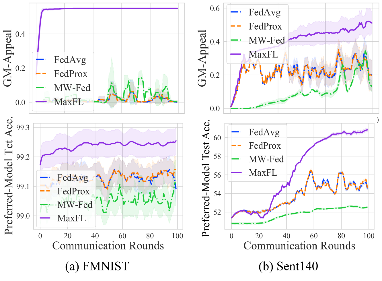
Figure 3: GM-Appeal (upper) and preferred-model test accuracy (lower) for the seen clients. For both datasets, the preferred-model test accuracy and GM-Appeal is significantly higher for MaxFL. Therefore, by using MaxFL, clients can also benefit from choosing either the local or global model for best performance, while the server also gains a large number of clients to select from.

	GM-Appeal		Preferred-Model Test Acc.
	FMNIST	Sent140	FMNIST	Sent140
FedAvg	$0.08{\scriptstyle(\pm 0.01)}$	$0.37{\scriptstyle(\pm 0.07)}$	$98.53{\scriptstyle(\pm 0.13)}$	$57.05{\scriptstyle(\pm 1.44)}$
FedProx	$0.07{\scriptstyle(\pm 0.01)}$	$0.37{\scriptstyle(\pm 0.07)}$	$98.43{\scriptstyle(\pm 0.21)}$	$57.07{\scriptstyle(\pm 1.42)}$
Scaffold	$0.02{\scriptstyle(\pm 0.01)}$	$0.03{\scriptstyle(\pm 0.05)}$	$98.26{\scriptstyle(\pm 0.20)}$	$51.59{\scriptstyle(\pm 0.11)}$
MW-Fed	$0.05{\scriptstyle(\pm 0.04)}$	$0.17{\scriptstyle(\pm 0.03)}$	$98.32{\scriptstyle(\pm 0.13)}$	$55.57{\scriptstyle(\pm 1.28)}$
MaxFL	$\mathbf{0.55}{\scriptstyle(\pm 0.0)}$	$\mathbf{0.43}{\scriptstyle(\pm 0.05)}$	$\mathbf{98.83}{\scriptstyle(\pm 0.06)}$	$\mathbf{57.16}{\scriptstyle(\pm 1.35)}$

Figure 4: GM-Appeal and preferred-model test accuracy of the final global models for the unseen clients’ test data that were not active during the training. MaxFL improves the GM-Appeal of the new incoming unseen clients by at least $47\%$ for FMNIST, and $6\%$ for Sent140 and achieves the same or higher preferred-model test accuracy compared to that of all baselines.

Robustness of MaxFL Against Byzantine Clients. One may think that MaxFL may be perceptible to attacks from Byzantine clients that intentionally send a greater GM-Appeal gap to the server to gain a higher aggregation weight. To show MaxFL’s robustness against such attacks we show in Table 2 the performance of MaxFL with Byzantine clients attacks which send higher losses to gain higher weights and then send Gaussian noise mixed gradients to the server. We compare with the MW-Fed baseline [16] which aims for incentivizing client participation by clients sending higher weights to the server and performing more local updates. In Table 2 we see that for both high and low byzantine client ratios, MaxFL achieves only $1$-$5\%$ lower test accuracy for seen and unseen clients compared to the case where there are no Byzantine clients in Table 1. This is due to our objective (3) giving lower weight to those clients that give a too high GM-Appeal gap (see Fig. 2). Hence while MW-Fed is susceptible to Byzantine attacks, MaxFL disregards these clients that send artificially high GM-Appeal gaps.

Preferred-model Test Accuracy: Clients’ Perspective.

In Fig. 4 and Fig. 4 we show the GM-Appeal and preferred-model test accuracy for the seen and unseen clients respectively. Recall that a high preferred-model test accuracy implies that the client has a higher chance in satisfying its requirement by choosing between the global or solo-trained local model, whichever performs better. First, in Fig. 4 we show that as the GM-Appeal increases across the communication round, preferred-model test accuracy also increases. Among the other baselines, MaxFL achieves the highest final GM-Appeal and preferred-model test accuracy. This indicates that MaxFL provides a win-win situation for both the server and the clients, since the clients have the highest accuracy by choosing the better model between the global model $\mathbf{w}$ and the local model $\widehat{\mathbf{w}}_{k}$, and the server has the highest fraction of participating clients. Similarly, in Fig. 4, we show that MaxFL achieves the highest GM-Appeal and preferred-model test accuracy. Although the preferred-model test accuracy improvement compared to the other baselines may appear small, showing that MaxFL is able to maintain a high preferred-model test accuracy while also achieving a high GM-Appeal implies that it does not sabotage the benefit of clients while also bringing the server more clients to select from.

	Seen Clients		Unseen Clients
	FMNIST	Sent140	FMNIST	Sent140
FedAvg	$0.38{\scriptstyle(\pm 0.06)}$	$0.25{\scriptstyle(\pm 0.09)}$	$0.39{\scriptstyle(\pm 0.06)}$	$0.42{\scriptstyle(\pm 0.06)}$
FedProx	$0.40{\scriptstyle(\pm 0.07)}$	$0.26{\scriptstyle(\pm 0.09)}$	$0.41{\scriptstyle(\pm 0.07)}$	$0.43{\scriptstyle(\pm 0.12)}$
Scaffold	$0.02{\scriptstyle(\pm 0.02)}$	$0.16{\scriptstyle(\pm 0.22)}$	$0.03{\scriptstyle(\pm 0.02)}$	$0.07{\scriptstyle(\pm 0.01)}$
PerFedAvg	$0.45{\scriptstyle(\pm 0.05)}$	$0.24{\scriptstyle(\pm 0.10)}$	$0.46{\scriptstyle(\pm 0.06)}$	$0.47{\scriptstyle(\pm 0.06)}$
MW-Fed	$0.28{\scriptstyle(\pm 0.07)}$	$0.08{\scriptstyle(\pm 0.01)}$	$0.39{\scriptstyle(\pm 0.04)}$	$0.20{\scriptstyle(\pm 0.01)}$
MaxFL	$\mathbf{0.55}{\scriptstyle(\pm 0.01)}$	$\mathbf{0.36}{\scriptstyle(\pm 0.05)}$	$\mathbf{0.56}{\scriptstyle(\pm 0.01)}$	$\mathbf{0.55}{\scriptstyle(\pm 0.01)}$

Table 3: GM-Appeal of locally-tuned models with 5 local steps from the final global models for seen clients and unseen clients. Both for clients that are active during training and unseen test clients, MaxFL increases the fraction of clients that find the global model appealing by at least $10\%$ as compared to all baselines.

Local Tuning for Personalization.

Personalized FL methods can be used to fine-tune the global model at each client before comparing it with the client’s locally trained model. MaxFL can be combined with these methods by simply allowing clients to perform some fine-tuning iterations before computing the aggregation weights in Step 7 of Algorithm 1. Both for clients that are active during training and unseen test clients, we show in Table 3 that MaxFL increases the GM-Appeal by at least $10\%$ compared to all baselines. For FMNIST and Sent140, the improvement in GM-Appeal over other methods is up to $27\%,\leavevmode\nobreak\ 28\%$ respectively for active clients and $17\%,\leavevmode\nobreak\ 4\%$ respectively for unseen clients.

6 Concluding Remarks

In this work, we aim to understand whether the global model can maximize the number of clients whose requirements are satisfied in FL, defining this via the novel notion of GM-Appeal. We show that when participating clients drop out or new clients do not join due to finding the global model less appealing, the test accuracy for the current training (seen) clients and generalization performance to the new unseen clients can suffer significantly. We show that our proposed MaxFL framework (with convergence guarantees) which aims to maximize the global model appeal, is able to retain many clients for training and thus achieves a high average test accuracy across the participating clients and also across the new incoming clients. Moreover, we show additional benefits of MaxFL such as being robust against Byzantine clients and improving the preferred-model test accuracy for the clients. A similar notion of global model appeal has not been properly examined before, and we expect our work to open up new research directions in understanding the role played by the server in preventing client dropout and recruiting new clients by finding a global model that can satisfy as many clients as possible.

Appendix A Toy Example: Mean Estimation for MaxFL

A.1 Maximizing GM-Appeal in Mean Estimation: Theoretical Analysis

We consider a setup with $M=2$ clients where the true loss function at each client is given by $f_{k}(w)=(w-\theta_{k})^{2}$. In practice, clients only have $N_{k}$ samples drawn from the distribution given by $e_{k,j}\sim\mathcal{N}(\theta_{k},\nu^{2}),\;\forall j\in[N_{k}]$. We further assume that the empirical loss function at each client is given by $F_{k}(w)=(w-\widehat{\theta}_{k})^{2}+(\widehat{\theta}_{k}-\theta_{k})^{2}$ where $\widehat{\theta}_{k}$ is the empirical mean, $\widehat{\theta}_{k}=\frac{1}{|\mathcal{B}_{k}|}\sum_{j=1}^{N_{k}}e_{k,j}$. It is easy to see that the minimizer of $F_{k}(w)$ is the empirical mean $\widehat{\theta}_{k}$. Thus, we set the solo-trained model at each client as $\widehat{w}_{k}=\widehat{\theta}_{k}$ and the loss threshold requirement at a client as $\rho_{k}=F_{k}(\widehat{w}_{k})=(\widehat{\theta}_{k}-\theta_{k})^{2}$.

GM-Appeal for Standard FL Model Decreases Exponentially with Heterogeneity. For simplicity let us assume $N_{1}=N_{2}=N$. Let $\gamma^{2}=\nu^{2}/N$ be the variance of the local empirical means and $\gamma_{G}^{2}=((\theta_{1}-\theta_{2})/2)^{2}>0$ be a measure of heterogeneity between the true means. The standard FL objective will always set the FL model to be the average of the local empirical means (i.e. $w=(\widehat{\theta}_{1}+\widehat{\theta}_{2})/2$) and does not take into account the heterogeneity among the clients. As a result, the GM-Appeal of the global model decreases exponentially as $\gamma_{G}^{2}$ increases.

Lemma A.1.

The expected GM-Appeal of the standard FL model is upper bounded by $2\exp\left(-\frac{\gamma_{G}^{2}}{5\gamma^{2}}\right)$, where the expectation is taken over the randomness in the local datasets $\mathcal{B}_{1},\mathcal{B}_{2}$.

Maximizing GM-Appeal with Relaxed Objective. We now explicitly maximize the GM-Appeal for this setting by solving for a relaxed version of the objective in 2 as proposed earlier. We replace the true loss $f_{k}(\cdot)$ by the empirical loss $F_{k}(\cdot)$ and replace the 0-1 (sign) loss with a differentiable approximation $h(\cdot)$.

We first show that setting $h(\cdot)$ to be a standard convex surrogate for the 0-1 loss (e.g. log loss, exponential loss, ReLU) leads to our new objective behaving the same as the standard FL objective.

Lemma A.2.

Let $h$ be any function that is convex, twice differentiable, and strictly increasing in $[0,\infty)$. Then our relaxed objective is strictly convex and has a unique minimizer at $w^{*}=\left(\frac{\widehat{\theta}_{1}+\widehat{\theta}_{2}}{2}\right)$.

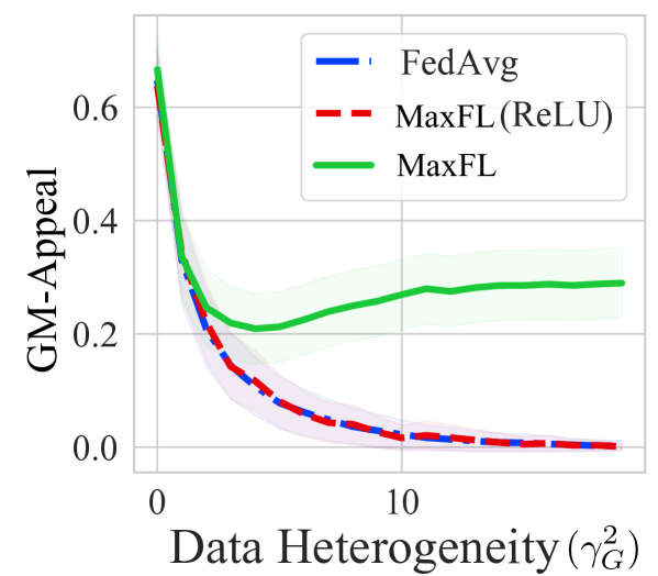
(a)

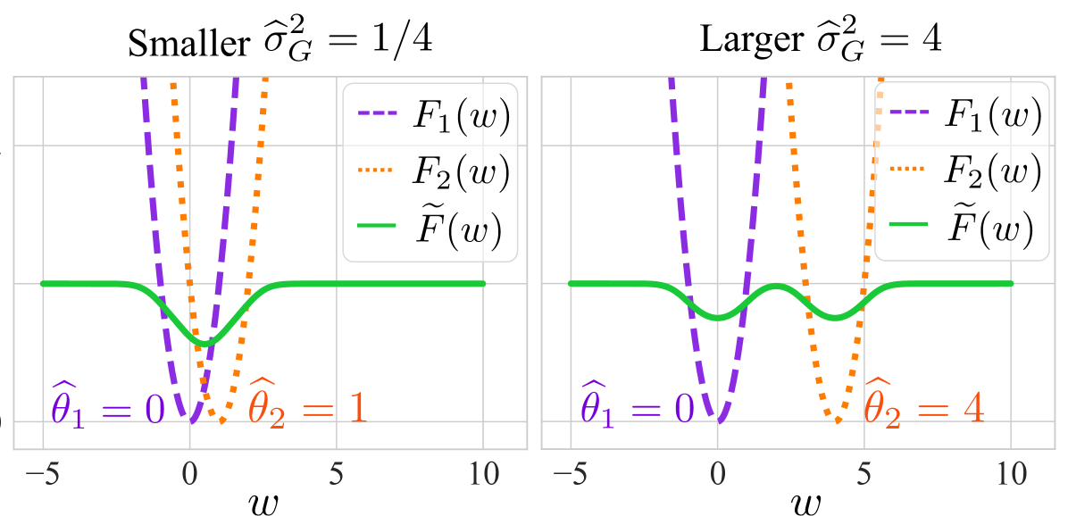
(b)

Figure 5: Results for the two client mean estimation; (a): GM-Appeal for FedAvg decays exponentially while GM-Appeal for MaxFL is lower bounded by a constant. Replacing the sigmoid approximation with ReLU approximation in MaxFL leads to the same solution as FedAvg; (b): MaxFL adapts to the heterogeneity of the problem—for small heterogeneity it encourages collaboration by having a single global minima, for large heterogeneity it encourages separation by having far away local minimas.

Maximizing the MaxFL Objective Leads to Increased GM-Appeal. Based on Lemma A.2, we see that we need nonconvexity in $h(\cdot)$ for the objective to behave differently than standard FL. We set $h(x)=\sigma(x)=\frac{\exp(x)}{1+\exp(x)}$, as proposed in our MaxFL objective in (3). We find that the MaxFL objective adapts to the empirical heterogeneity parameter $\widehat{\gamma}_{G}^{2}=\left(\frac{\widehat{\theta}_{2}-\widehat{\theta}_{1}}{2}\right)^{2}$. If $\widehat{\gamma}_{G}^{2}<1$ (small data heterogeneity), the objective encourages collaboration by setting the global model to be the average of the local models. On the other hand, if $\widehat{\gamma}_{G}^{2}>2$ (large data heterogeneity), the objective encourages separation by setting the global model close to either the local model of the first client or the local model of the second client (see Fig. 5). Based on this observation, we have the following theorem.

Theorem A.1.

Let $w$ be a local minima of the MaxFL objective. The expected GM-Appeal using $w$ is lower bounded by $\frac{1}{16}\exp\left(-\frac{1}{\gamma^{2}}\right)$where the expectation is over the randomness in the local dataset $\mathcal{B}_{1},\mathcal{B}_{2}$.

Note that our result above is independent of the heterogeneity parameter $\gamma_{G}^{2}$. Therefore even with $\gamma_{G}^{2}\gg 0$, MaxFL will keep incentivizing atleast one client by adapting its objective accordingly. Additional discussion and proof details can be found in Section A.2.

Mean Estimation with 3 Clients with MaxFL. We further examine the property of MaxFL to satisfy clients with a 3 clients toy example which is an extension from what we have shown for 2 clients. Reusing the notation from the 2 client example, where $\theta_{i}$ is the true mean at client $i$ and $\hat{\theta}_{i}\sim\mathcal{N}(\theta_{i},1)$ is the empirical mean of a client, our analysis can be divided into the following cases for the 3 client example (see Fig. 6):

• Case 1: $\theta_{1}\approx\theta_{2}\approx\theta_{3}$: This case captures the setting where the data at the clients is almost i.i.d. In this case, it makes sense for clients to collaborate together and therefore MaxFL’s optimal solution will be the average of local empirical means (same as FedAvg).

• Case 2: $\theta_{1}\neq\theta_{2}\neq\theta_{3}$: This case captures the setting where the data at clients is completely disparate. In this case, none of the clients benefit from collaborating and therefore MaxFL’s optimal solution will be the local model of one of the clients. This ensures at least one of the clients will still be satisfied with the MaxFL global model unlike FedAvg.

• Case 3: $\theta_{1}\approx\theta_{2}\neq\theta_{3}$: The most interesting case happens when data at two of the clients is similar but the data at the third client is different. Without loss of generality we assume that data at clients 1 and 2 is similar and client 3 is different. In this case, although client 1 and 2 benefit from federating, FedAvg is unable to leverage that due to the heterogeneity at client 3. MaxFL, on the other hand, will set the optimal solution to be the average of the local models of just client 1 and client 2. This ensures clients 1 and 2 are satisfied with the global model, thus maximizing the GM-Appeal.

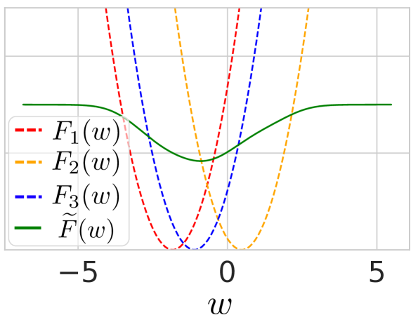
(a)

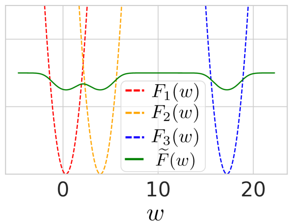
(b)

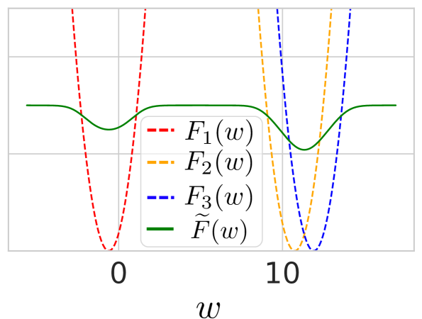
(c)

Figure 6: Results for the three client mean estimation; (a): case 1 when the true mean across clients are close to amongst each other where MaxFL’s optimal solution is identical to that of FedAvg; (b): case 2 when the true mean across clients are all different from each other where MaxFL’s optimal solution ensures that at least one of the clients will be satisfied with MaxFL’s global model (unlike FedAvg); (c) case 3 when two clients’ true means are close to each other while the other client has a different mean. MaxFL in this case, is able to ensure that the two clients satisfied while FedAvg is not able to make any client satisfied.

The behavior of MaxFL in the three client setup clearly highlights the non-trivialness of our proposed MaxFL’s formulation.

A.2 Proof for Theoretical Analysis in Section A.1

Recall the setup discussed in Section A.1. We additionally define the following quantities

$$\gamma^{2}\vcentcolon=\frac{\nu^{2}}{N};\hskip 10.0pt\gamma^{2}_{G}=\left(\frac{\theta_{2}-\theta_{1}}{2}\right)^{2};$$ (8)

Note that the distribution of the empirical means itself follows a normal distribution following the linear additivity of independent normal random variables.

$$\widehat{\theta}_{1}\sim\mathcal{N}(\theta_{1},\gamma^{2});\hskip 10.0pt\widehat{\theta}_{2}\sim\mathcal{N}(\theta_{2},\gamma^{2})$$ (9)

Lemma A.1 The expected GM-Appeal of the standard FL model is upper bounded by $2\exp\left(-\frac{\gamma_{G}^{2}}{5\gamma^{2}}\right)$, where the expectation is taken over the randomness in the local datasets $\mathcal{B}_{1},\mathcal{B}_{2}$.

Proof.

The standard FL model is given by,

$$w=\frac{\widehat{\theta}_{1}+\widehat{\theta}_{2}}{2}$$ (10)

Therefore the expected GM-Appeal is,

$$\mathbb{E}\left[{\frac{\mathbb{I}\{(w-\theta_{1})^{2}<(\widehat{\theta}_{1}-\theta_{1})^{2}\}+\mathbb{I}\{(w-\theta_{2})^{2}<(\widehat{\theta}_{2}-\theta_{2})^{2}\}}{2}}\right]$$ (11)

$$=\frac{1}{2}\left[\underbrace{\mathbb{P}\left({(w-\theta_{1})^{2}<(\widehat{\theta}_{1}-\theta_{1})^{2}}\right)}_{T_{1}}+\underbrace{\mathbb{P}\left({(w-\theta_{2})^{2}<(\widehat{\theta}_{2}-\theta_{2})^{2}}\right)}_{T_{2}}\right]$$ (12)

Next we bound $T_{1}$ and $T_{2}$.

$$T_{1} =\mathbb{P}\left({(w-\theta_{1})^{2}<(\widehat{\theta}_{1}-\theta_{1})^{2}}\right)$$ (13)

$$=\mathbb{P}\left({\left({\frac{\widehat{\theta}_{1}+\widehat{\theta}_{2}}{2}-\theta_{1}}\right)^{2}<(\widehat{\theta}_{1}-\theta_{1})^{2}}\right)$$ (14)

$$=\mathbb{P}\left({\left({\frac{\widehat{\theta}_{2}-\widehat{\theta}_{1}}{2}}\right)^{2}+2\left({\frac{\widehat{\theta}_{2}-\widehat{\theta}_{1}}{2}}\right)(\widehat{\theta}_{1}-\theta_{1})<0}\right)$$ (15)

$$=\mathbb{P}\left({\left\{\left({\frac{\widehat{\theta}_{2}-\widehat{\theta}_{1}}{2}}\right)^{2}+2\left({\frac{\widehat{\theta}_{2}-\widehat{\theta}_{1}}{2}}\right)(\widehat{\theta}_{1}-\theta_{1})<0\right\}\cap\left\{\widehat{\theta}_{2}>\widehat{\theta}_{1}\right\}}\right)$$

$$\hskip 10.0pt+\mathbb{P}\left({\left\{\left({\frac{\widehat{\theta}_{2}-\widehat{\theta}_{1}}{2}}\right)^{2}+2\left({\frac{\widehat{\theta}_{2}-\widehat{\theta}_{1}}{2}}\right)(\widehat{\theta}_{1}-\theta_{1})<0\right\}\cap\left\{\widehat{\theta}_{2}\leq\widehat{\theta}_{1}\right\}}\right)$$ (16)

$$=\mathbb{P}\left({\left\{\left({\frac{\widehat{\theta}_{2}-\widehat{\theta}_{1}}{2}}\right)+2(\widehat{\theta}_{1}-\theta_{1})<0\right\}\cap\left\{\widehat{\theta}_{2}>\widehat{\theta}_{1}\right\}}\right)$$

$$\hskip 10.0pt+\mathbb{P}\left({\left\{\left({\frac{\widehat{\theta}_{2}-\widehat{\theta}_{1}}{2}}\right)^{2}+2\left({\frac{\widehat{\theta}_{2}-\widehat{\theta}_{1}}{2}}\right)(\widehat{\theta}_{1}-\theta_{1})<0\right\}\cap\left\{\widehat{\theta}_{2}\leq\widehat{\theta}_{1}\right\}}\right)$$ (17)

$$\leq\mathbb{P}\left({\left({\frac{\widehat{\theta}_{2}-\widehat{\theta}_{1}}{2}}\right)+2(\widehat{\theta}_{1}-\theta_{1})<0}\right)+\mathbb{P}\left({\widehat{\theta}_{2}-\widehat{\theta}_{1}\leq 0}\right)$$ (18)

$$=\mathbb{P}\left({Z_{1}<0}\right)+\mathbb{P}\left({Z_{2}\leq 0}\right)\hskip 5.0pt\text{ where }Z_{1}\sim\mathcal{N}\left(\gamma_{G},\frac{5}{2}\gamma^{2}\right),Z_{2}\sim\mathcal{N}\left(2\gamma_{G},2\gamma^{2}\right)$$ (19)

$$\leq\exp\left({-\frac{\gamma_{G}^{2}}{5\gamma^{2}}}\right)+\exp\left({-\frac{\gamma_{G}^{2}}{\gamma^{2}}}\right)$$ (20)

$$\leq 2\exp\left({-\frac{\gamma_{G}^{2}}{5\gamma^{2}}}\right)$$ (21)

where 16 uses $\mathbb{P}\left({A}\right)=\mathbb{P}\left({A\cap B}\right)+\mathbb{P}\left({A\cap B^{\complement}}\right)$, 18 uses $\mathbb{P}\left({A\cap B}\right)\leq\mathbb{P}\left({A}\right)$, 19 uses 9 and linear additivity of independent normal random variables, 20 uses a Chernoff bound.

We can similarly bound $T_{2}$ to get $T_{2}\leq 2\exp\left({-\frac{\gamma_{G}^{2}}{5\gamma^{2}}}\right)$. Thus the expected GM-Appeal of the standard FL model is upper bounded by $2\exp\left({-\frac{\gamma_{G}^{2}}{5\gamma^{2}}}\right)$.

Lemma A.2 Let $h$ be any function that is convex, twice differentiable, and strictly increasing in $[0,\infty)$. Then our relaxed objective is strictly convex and has a unique minimizer at $w^{*}=\left(\frac{\widehat{\theta}_{1}+\widehat{\theta}_{2}}{2}\right)$.

Proof.

Let us denote our relaxed objective by $v(w)$. Then $v(w)$ can be written as,

$$v(w) =\frac{1}{2}\left[h\left(F_{1}(w)-F(\widehat{w}_{1})\right)+h\left(F_{2}(w)-F(\widehat{w}_{2})\right)\right]=\underbrace{\frac{1}{2}h\left((w-\widehat{\theta}_{1})^{2}\right)}_{v_{1}(w)}+\underbrace{\frac{1}{2}h\left((w-\widehat{\theta}_{2})^{2}\right)}_{v_{2}(w)}$$ (22)

We first prove that $v_{1}(w)$ is strictly convex. Let $\lambda\in(0,1)$ and $(w_{1},w_{2})$ be any pair of points in $\mathbb{R}^{2}$ such that $w_{1}\neq w_{2}$. We have,

$$v_{1}(\lambda w_{1}+(1-\lambda)w_{2}) =\frac{1}{2}h\left((\lambda(w_{1}-\widehat{\theta}_{1})+(1-\lambda)(w_{2}-\widehat{\theta}_{1}))^{2}\right)$$ (24)

$$<\frac{1}{2}h\left(\lambda(w_{1}-\widehat{\theta}_{1})^{2}+(1-\lambda)(w_{2}-\widehat{\theta}_{1})^{2}\right)$$ (25)

$$\leq\frac{\lambda}{2}h\left((w_{1}-\widehat{\theta}_{1})^{2}\right)+\frac{1-\lambda}{2}h\left((w_{2}-\widehat{\theta}_{1})^{2}\right)$$ (26)

$$=\lambda v_{1}(w_{1})+(1-\lambda)v_{1}(w_{2})$$ (27)

where 25 follows from the strict convexity of $f(w)=w^{2}$ and the fact that $h(w)$ is strictly increasing in the range $[0,\infty)$, 26 follows from the convexity of $h(w)$.

This completes the proof that $v_{1}(w)$ is strictly convex. We can similarly prove that $v_{2}(w)$ is stricly convex and hence $v(w)$ is strictly convex since summation of strictly convex functions is strictly convex.

Also note that,

$$\nabla v(w)=\nabla h\left((w-\widehat{\theta}_{1})^{2}\right)(w-\widehat{\theta}_{1})+\nabla h\left((w-\widehat{\theta}_{2})^{2}\right)(w-\widehat{\theta}_{2})$$ (28)

It is easy to see that $\nabla v(w)=0$ at $w=\left(\frac{\widehat{\theta}_{1}+\widehat{\theta}_{2}}{2}\right)$. Since $v(w)$ is strictly convex this implies that $w^{*}=\left(\frac{\widehat{\theta}_{1}+\widehat{\theta}_{2}}{2}\right)$ will be a unique global minimizer. This completes the proof.

Proof of Theorem A.1

Before stating the proof of Theorem A.1 we first state some intermediate results that will be used in the proof.

The MaxFL objective can be written as,

$$v(w)=\frac{1}{2}\sigma\left({(w-\widehat{\theta}_{1})^{2}}\right)+\frac{1}{2}\sigma\left({(w-\widehat{\theta}_{2})^{2}}\right)$$ (29)

where $\sigma(w)=1/(1+\exp(-w))$.

We additionally define the following quantities,

$$i\vcentcolon=\operatorname*{argmin}\left\{\widehat{\theta}_{1},\widehat{\theta}_{2}\right\};\hskip 5.0ptj\vcentcolon=\operatorname*{argmax}\left\{\widehat{\theta}_{1},\widehat{\theta}_{2}\right\};\hskip 5.0pt\widehat{\gamma}_{G}\vcentcolon=\frac{\widehat{\theta}_{j}-\widehat{\theta}_{i}}{2}$$ (30)

Let $q(w)=\sigma(w)(1-\sigma(w))$. The gradient of $v(w)$ is given as,

$$\nabla v(w)=q\left((w-\widehat{\theta}_{1})^{2}\right)(w-\widehat{\theta}_{1})+q\left((w-\widehat{\theta}_{2})^{2}\right)(w-\widehat{\theta}_{2})$$ (31)

Lemma A.3 For $\widehat{\gamma}_{G}>2$, $w=\left(\frac{\widehat{\theta}_{1}+\widehat{\theta}_{2}}{2}\right)$ will be a local maxima of the MaxFL objective.

It is easy to see that $w=\left(\frac{\widehat{\theta}_{1}+\widehat{\theta}_{2}}{2}\right)$ will always be a stationary point of $\nabla v(w)$. Our goal is to determine whether it will be a local minima or a local maxima. To do so, we calculate the hessian of $v(w)$ as follows. Let $f(w)=2\sigma(w)(1-\sigma(w))(1-2\sigma(w))$. Then,

$$\nabla^{2}v(w)=\underbrace{f\left((w-\widehat{\theta}_{1})^{2}\right)(w-\widehat{\theta}_{1})^{2}+q\left((w-\widehat{\theta}_{1})^{2}\right)}_{h_{1}(w)}+\underbrace{f\left((w-\widehat{\theta}_{2})^{2}\right)(w-\widehat{\theta}_{2})^{2}+q\left((w-\widehat{\theta}_{2})^{2}\right)}_{h_{2}(w)}$$ (32)

Note that $h_{1}(w)=h_{2}(w)$ for $w=\left(\frac{\widehat{\theta}_{1}+\widehat{\theta}_{2}}{2}\right)$. Hence it suffices to focus on the condition for which $h_{1}(w)<0$ at $w=\left(\frac{\widehat{\theta}_{1}+\widehat{\theta}_{2}}{2}\right)$. We have,

$$h_{1}\left((\widehat{\theta}_{1}+\widehat{\theta}_{2})/2\right) =f(\widehat{\gamma}_{G}^{2})\widehat{\gamma}_{G}^{2}+q(\widehat{\gamma}_{G}^{2})$$ (33)

$$=q(\widehat{\gamma}_{G}^{2})(2(1-2\sigma(\widehat{\gamma}_{G}^{2}))\widehat{\gamma}_{G}^{2}+1)$$ (34)

$$<0\hskip 5.0pt\text{ for }\widehat{\gamma}_{G}\geq 1.022$$ (35)

where the last inequality follows from the fact that $q(w)>0$ for all $w\in\mathbb{R}$ and $2(1-2\sigma(w^{2}))w^{2}+1<0$ for $w\geq 1.022$. Thus for $\widehat{\gamma}_{G}>2$, $w=\left(\frac{\widehat{\theta}_{1}+\widehat{\theta}_{2}}{2}\right)$ will be a local maxima of the MaxFL objective.

Lemma A.4 For $\widehat{\gamma}_{G}>0$, any local minima of $v(w)$ lies in the range $(\widehat{\theta}_{i},\widehat{\theta}_{i}+2]\cup[\widehat{\theta}_{j}-2,\widehat{\theta}_{j})$.

Firstly note that since $\widehat{\gamma}_{G}>0$ we have $\widehat{\theta}_{j}>\widehat{\theta}_{i}$. Secondly note that since $q(w)>0$ for all $w\in\mathbb{R}$, $\nabla v(w)<0$ for all $w\leq\widehat{\theta}_{i}$ and $\nabla v(w)>0$ for all $w\geq\widehat{\theta}_{j}$. Therefore any root of the function $\nabla v(w)$ must lie in the range $(\widehat{\theta}_{i},\widehat{\theta}_{j})$.

Case 1: $0<\widehat{\gamma}_{G}\leq 2$.

In this case, the lemma is trivially satisified since $(\widehat{\theta}_{i},\widehat{\theta}_{j})\subset\left\{(\widehat{\theta}_{i},\widehat{\theta}_{i}+2]\cup[\widehat{\theta}_{j}-2,\widehat{\theta}_{j})\right\}$.

Case 2: $\widehat{\gamma}_{G}>2$.

Let $x=w-\widehat{\theta}_{i}$ and $g(x)=q(x^{2})x$. We can write $\nabla v(w)$ as,

$$\nabla v(\widehat{\theta}_{i}+x)=g(x)-g(2\widehat{\gamma}_{G}-x)$$ (36)

It can be seen that for $x>2$, $g(x)$ is a decreasing function. For $x\in(2,\widehat{\gamma}_{G})$ we have $x>2\widehat{\gamma}_{G}-x$ which implies $g(x)>g(2\widehat{\gamma}_{G}-x)$. Therefore $\nabla v(\widehat{\theta}_{i}+x)>0$ for $x\in(2,\widehat{\gamma}_{G})$. Also $\nabla v(\widehat{\theta}_{i}+2\widehat{\gamma}_{G}-x)=-\nabla v(\widehat{\theta}_{i}+x)$ and therefore $\nabla v(\widehat{\theta}_{i}+x)<0$ for $x\in(\widehat{\gamma}_{G},2\widehat{\gamma}_{G}-2)$. $\nabla v(\widehat{\theta}_{i}+\widehat{\gamma}_{G})=0$ but this will be a local maxima for $\widehat{\gamma}_{G}>2$ as shown in Lemma A.3. Thus there exists no local minima of $v(w)$ for $w\in(\widehat{\theta}_{i}+2,\widehat{\theta}_{j}-2)$

Combining both cases we see that any local minima of $v(w)$ lies in the range $\left\{(\widehat{\theta}_{i},\widehat{\theta}_{i}+2]\cup[\widehat{\theta}_{j}-2,\widehat{\theta}_{j})\right\}$.

Theorem A.1 Let $w$ be a local minima of the MaxFL objective. The expected GM-Appeal using $w$ is lower bounded by $\frac{1}{16}\exp\left(-\frac{1}{\gamma^{2}}\right)$ where the expectation is over the randomness in the local dataset $\mathcal{B}_{1},\mathcal{B}_{2}$.

Proof.

The GM-Appeal can be written as,

$$\frac{1}{2}\left[\mathbb{P}\left({(w-\theta_{i})^{2}<(\widehat{\theta}_{i}-\theta_{i})^{2}}\right)+\mathbb{P}\left({(w-\theta_{j})^{2}<(\widehat{\theta}_{j}-\theta_{j})^{2}}\right)\right]$$ (37)

We focus on the case where $\widehat{\theta}_{2}\neq\widehat{\theta}_{i}$ implying $\widehat{\theta}_{j}>\widehat{\theta}_{i}$ ($\widehat{\theta}_{2}=\widehat{\theta}_{1}$ is a zero-probability event and does not affect our proof). Let $w$ be any local minima of the MaxFL objective. From Lemma A.4 we know that $w$ will lie in the range $(\widehat{\theta}_{i},\widehat{\theta}_{i}+2]\cup[\widehat{\theta}_{j}-2,\widehat{\theta}_{j})$

Case 1: $w\in(\widehat{\theta}_{i},\widehat{\theta}_{i}+2]$

$$\mathbb{P}\left({(w-\theta_{i})^{2}<(\widehat{\theta}_{i}-\theta_{i})^{2}}\right) =\mathbb{P}\left({(w-\widehat{\theta}_{i})^{2}+2(w-\widehat{\theta}_{i})(\widehat{\theta}_{i}-\theta_{i})<0}\right)$$ (38)

$$=\mathbb{P}\left({(w-\widehat{\theta}_{i})+2(\widehat{\theta}_{i}-\theta_{i})<0}\right)$$ (39)

$$\geq\mathbb{P}\left({2+2(\widehat{\theta}_{i}-\theta_{i})<0}\right)$$ (40)

$$=\mathbb{P}\left({(\widehat{\theta}_{i}-\theta_{i})<-1}\right)$$ (41)

$$\geq\mathbb{P}\left({\left\{\widehat{\theta}_{1}<\widehat{\theta}_{2}\right\}\cap\left\{(\widehat{\theta}_{1}-\theta_{1})<-1\right\}}\right)$$ (42)

$$=\mathbb{P}\left({\widehat{\theta}_{1}<\widehat{\theta}_{2}}\right)\mathbb{P}\left({\widehat{\theta}_{1}-\theta_{1}<-1|\widehat{\theta}_{1}<\widehat{\theta}_{2}}\right)$$ (43)

$$\geq\mathbb{P}\left({\widehat{\theta}_{1}<\widehat{\theta}_{2}}\right)\mathbb{P}\left({\widehat{\theta}_{1}-\theta_{1}<-1}\right)$$ (44)

$$=\mathbb{P}\left({\widehat{\theta}_{1}<\widehat{\theta}_{2}}\right)\mathbb{P}\left({Z>1/\gamma}\right)\hskip 5.0pt\text{ where }Z\sim\mathcal{N}(0,1)$$ (45)

$$\geq\frac{1}{8}\exp\left(-\frac{1}{\gamma^{2}}\right)$$ (46)

39 uses the fact that $(w-\widehat{\theta}_{i})>0$, 40 uses $(w-\widehat{\theta}_{i})\leq 2$, 42 uses $\mathbb{P}\left({A}\right)\geq\mathbb{P}\left({A\cap B}\right)$ and definition of $i$. 44 uses the following argument. If $\theta_{1}-1\geq\widehat{\theta}_{2}$ then $\mathbb{P}\left({\widehat{\theta}_{1}-\theta_{1}<-1|\widehat{\theta}_{1}<\widehat{\theta}_{2}}\right)=1$. If $\theta_{1}-1<\widehat{\theta}_{2}$ then $\mathbb{P}\left({\widehat{\theta}_{1}-\theta_{1}<-1|\widehat{\theta}_{1}<\widehat{\theta}_{2}}\right)=\mathbb{P}\left({\widehat{\theta}_{1}-\theta_{1}<-1}\right)/\mathbb{P}\left({\widehat{\theta}_{1}<\widehat{\theta}_{2}}\right)\geq\mathbb{P}\left({\widehat{\theta}_{1}-\theta_{1}<-1}\right)$. 45 uses $\widehat{\theta}_{1}-\theta_{1}\sim\mathcal{N}(0,\gamma^{2})$, 46 uses $\mathbb{P}\left({\widehat{\theta}_{1}<\widehat{\theta}_{2}}\right)\geq\frac{1}{2}$ and $\mathbb{P}\left({Z\geq x}\right)\geq\frac{2\exp(-x^{2}/2)}{\sqrt{2\pi}(\sqrt{4+x^{2}}+x)}\geq\frac{1}{4}\exp(-x^{2})$ where $Z\sim\mathcal{N}(0,1)$ [33].

In the case where $w\in(\widehat{\theta}_{j}-2,\widehat{\theta}_{j}]$ a similar technique can be used to lower bound $\mathbb{P}\left({(w-\theta_{j})^{2}<(\widehat{\theta}_{j}-\theta_{j})^{2}}\right)$. Thus the GM-Appeal of any local minima of the MaxFL objective is lower bounded by $\frac{1}{16}\exp\left(-\frac{1}{\gamma^{2}}\right)$.

Appendix B Convergence Proof

B.1 Preliminaries

First, we introduce the key lemmas used for the convergence analysis.

Lemma B.1 (Bounded Dissimilarity for $\widetilde{F}(\mathbf{w})$).

With 3.1 and 3.3 we have the bounded dissimilarity with respect to $\widetilde{F}(\mathbf{w})$ as:

$$\frac{1}{M}\sum_{i=1}^{M}\|\nabla\widetilde{F}_{i}(\mathbf{w})\|^{2}\leq\beta^{\prime 2}\|\nabla\widetilde{F}(\mathbf{w})\|^{2}+\kappa^{\prime 2}$$ (47)

where $\beta^{\prime 2}=2\beta^{2},\leavevmode\nobreak\ \kappa^{\prime 2}=4\beta^{2}L_{c}^{2}+\kappa^{2}$

Proof.

One can easily show that

$$\frac{1}{M}\sum_{i=1}^{M}\|\nabla\widetilde{F}_{i}(\mathbf{w})\|^{2}=\frac{1}{M}\sum_{i=1}^{M}q_{i}(\mathbf{w})^{2}\|\nabla{F}_{i}(\mathbf{w})\|^{2}\leq\frac{1}{M}\sum_{i=1}^{M}\|\nabla F_{i}(\mathbf{w})\|^{2}$$ (48)

due to $q_{i}(\mathbf{w})\leq 1$. Hence we have from 3.3 and Cauchy-Schwarz inequality that

$$\frac{1}{M}\sum_{i=1}^{M}\|\nabla\widetilde{F}_{i}(\mathbf{w})\|^{2}\leq\frac{1}{M}\sum_{i=1}^{M}\|\nabla F_{i}(\mathbf{w})\|^{2}$$ (49)

$$\leq\beta^{2}\|\nabla F(\mathbf{w})-\nabla\widetilde{F}(\mathbf{w})+\nabla\widetilde{F}(\mathbf{w})\|^{2}+\kappa^{2}$$ (50)

$$\leq 2\beta^{2}\|\nabla F(\mathbf{w})-\nabla\widetilde{F}(\mathbf{w})\|^{2}+2\beta^{2}\|\nabla\widetilde{F}(\mathbf{w})\|^{2}+\kappa^{2}$$ (51)

We bound the first term in 51 as

$$\|\nabla F(\mathbf{w})-\nabla\widetilde{F}(\mathbf{w})\|^{2}=\left\|\sum_{i=1}^{M}\frac{(1-q_{i}(\mathbf{w}))}{M}\nabla F_{i}(\mathbf{w})\right\|^{2}$$ (52)

$$\leq\frac{1}{M}\sum_{i=1}^{M}\|(1-q_{i}(\mathbf{w}))\nabla F_{i}(\mathbf{w})\|^{2}$$ (53)

$$\leq\frac{2}{M}\sum_{i=1}^{M}\|\nabla F_{i}(\mathbf{w})\|^{2}\leq 2L_{c}^{2}$$ (54)

where in 54 we use $q_{i}(\mathbf{w})\leq 1,\forall i\in[M]$ and 3.1. Then from 51 we have

$$\frac{1}{M}\sum_{i=1}^{M}\|\nabla\widetilde{F}_{i}(\mathbf{w})\|^{2}\leq 2\beta^{2}\|\nabla\widetilde{F}(\mathbf{w})\|^{2}+\kappa^{2}+4\beta^{2}L_{c}^{2}$$ (55)

completing the proof. ∎

Lemma B.2 (Smoothness of $\widetilde{F}(\mathbf{w})$).

If 3.1 is satisfied we have that the local objectives, $\widetilde{F}_{1}(\mathbf{w}),\leavevmode\nobreak\ ...\leavevmode\nobreak\ ,\widetilde{F}_{M}(\mathbf{w})$, are also $\widetilde{L}_{s}$-smooth for any $\mathbf{w}$ where $\widetilde{L}_{s}=L_{c}^{2}/4+q_{i}({\bf w})L_{s}$.

Proof.

Recall the definitions of $\widetilde{F}(\mathbf{w})$ below:

$$\widetilde{F}(\mathbf{w})=\frac{1}{M}\sum_{i=1}^{M}\widetilde{F}_{i}(\mathbf{w}),\leavevmode\nobreak\ \widetilde{F}_{i}(\mathbf{w})\vcentcolon=\sigma(F_{i}(\mathbf{w})-F_{i}(\widehat{\mathbf{w}}_{i}^{*}))$$ (56)

Let $\|\hskip 1.0pt\|_{op}$ denote the spectral norm of a matrix. Accordingly, with the model parameter vector $\mathbf{w}\in\mathbb{R}^{d}$, we have the spectral norm of the Hessian of $\widetilde{F}_{i}(\mathbf{w}),\leavevmode\nobreak\ \forall i\in[M]$ as:

$$\begin{aligned} &\|\nabla^{2}\widetilde{F}_{i}(\mathbf{w})\|_{op}\\ &=\|q_{i}(\mathbf{w})[(\nabla F_{i}(\mathbf{w})\nabla F_{i}(\mathbf{w})^{T})(1-q_{i}(\mathbf{w}))+\nabla^{2}F_{i}(\mathbf{w})]\|_{op}\end{aligned}$$ (57)

where $q_{i}(\mathbf{w})=\text{Sigmoid}(F_{i}(\mathbf{w})-F_{i}(\widehat{\mathbf{w}}_{i}^{*}))$ and $\nabla F_{i}(\mathbf{w})\in\mathbb{R}^{d\times 1}$ is the gradient vector for the local objective $F_{i}(\mathbf{w})$ and $\nabla^{2}F_{i}(\mathbf{w})\in\mathbb{R}^{d\times d}$ is the Hessian of $F_{i}(\mathbf{w})$. We can bound the RHS of 57 as follows

$$\|\nabla^{2}\widetilde{F}_{i}(\mathbf{w})\|_{op}=\|q_{i}({\bf w})(1-q_{i}(\mathbf{w}))(\nabla F_{i}(\mathbf{w})\nabla F_{i}(\mathbf{w})^{T})+q_{i}({\bf w})\nabla^{2}F_{i}(\mathbf{w})]\|_{op}$$ (58)

$$\leq\|q_{i}({\bf w})(1-q_{i}(\mathbf{w}))(\nabla F_{i}(\mathbf{w})\nabla F_{i}(\mathbf{w})^{T})\|_{op}+\|q_{i}({\bf w})\nabla^{2}F_{i}(\mathbf{w})\|_{op}$$ (59)

$$=q_{i}({\bf w})(1-q_{i}(\mathbf{w}))\|(\nabla F_{i}(\mathbf{w})\nabla F_{i}(\mathbf{w})^{T})\|_{op}+q_{i}({\bf w})\|\nabla^{2}F_{i}(\mathbf{w})\|_{op}$$ (60)

$$=q_{i}({\bf w})(1-q_{i}(\mathbf{w}))\|\nabla F_{i}(\mathbf{w})\|^{2}+q_{i}({\bf w})\|\nabla^{2}F_{i}(\mathbf{w})\|_{op}$$ (61)

$$\leq\frac{L_{c}^{2}}{4}+q_{i}({\bf w})L_{s}$$ (62)

where we use triangle inequality in 59, and use $\|{\bf x}{\bf y}^{T}\|_{op}=\|{\bf x}\|\|{\bf y}\|$ in 61, and use $q_{i}(\mathbf{w})\leq 1$ along with 3.1 in 62. Since the norm of the Hessian of $\widetilde{F}_{i}(\mathbf{w})$ is bounded by $\frac{L_{c}^{2}}{4}+q_{i}({\bf w})L_{s}$ we complete the proof. ∎

B.2 Proof of Theorem 3.1 – Full Client Participation

For ease of writing, we define the following auxiliary variables for any client $i\in[M]$:

$$\text{Weighted Stochastic Gradient: }\mathbf{h}_{i}^{(t,0)}\vcentcolon=q_{i}(\mathbf{w}^{(t,0)})\sum_{r=0}^{\tau-1}\mathbf{g}(\mathbf{w}_{i}^{(t,r)},\xi_{i}^{(t,r)}),$$ (63)

$$\text{Weighted Gradient: }\overline{\mathbf{h}}_{i}^{(t,0)}\vcentcolon=q_{i}(\mathbf{w}^{(t,0)})\sum_{r=0}^{\tau-1}\nabla F_{i}(\mathbf{w}_{i}^{(t,r)}),$$ (64)

$$\text{Normalized Global Learning Rate: }\eta_{g}^{(t,0)}\vcentcolon=\eta_{g}/\left(\sum_{i=1}^{M}q_{i}(\mathbf{w}^{(t,0)})+\epsilon\right)$$ (65)

where $\epsilon$ is a constant added to the denominator to prevent the denominator from being $0$. From Algorithm 1 with full client participation, our proposed algorithm has the following effective update rule for the global model at the server:

$$\mathbf{w}^{(t+1,0)}=\mathbf{w}^{(t,0)}-\eta^{(t,0)}_{g}\eta_{l}\sum_{k=1}^{M}\mathbf{h}_{k}^{(t,0)}$$ (66)

With the update rule in 66, defining $\widetilde{\eta}^{(t,0)}\vcentcolon=\eta_{g}^{(t,0)}\eta_{l}\tau M$ and using Lemma B.2 we have

$$\begin{aligned} \mathbb{E}\left[\widetilde{F}(\mathbf{w}^{(t+1,0)})\right]-\widetilde{F}(\mathbf{w}^{(t,0)})\leq-\widetilde{\eta}^{(t,0)}\mathbb{E}\left[\left\langle\nabla\widetilde{F}(\mathbf{w}^{(t,0)}),\frac{1}{M\tau}\sum_{i=1}^{M}\mathbf{h}_{i}^{(t,0)}\right\rangle\right]\\ +\frac{\widetilde{L}_{s}(\widetilde{\eta}^{(t,0)})^{2}}{2}\mathbb{E}\left[\left\|\frac{1}{M\tau}\sum_{i=1}^{M}\mathbf{h}_{i}^{(t,0)}\right\|^{2}\right]\end{aligned}$$ (67)

$$\begin{aligned} =-\widetilde{\eta}^{(t,0)}\mathbb{E}\left[\left\langle\nabla\widetilde{F}(\mathbf{w}^{(t,0)}),\frac{1}{M\tau}\sum_{i=1}^{M}\left(\mathbf{h}_{i}^{(t,0)}-\overline{\mathbf{h}}_{i}^{(t,0)}\right)\right\rangle\right]-\widetilde{\eta}^{(t,0)}\mathbb{E}\left[\left\langle\nabla\widetilde{F}(\mathbf{w}^{(t,0)}),\frac{1}{M\tau}\sum_{i=1}^{M}\overline{\mathbf{h}}_{i}^{(t,0)}\right\rangle\right]\\ +\frac{\widetilde{L}_{s}(\widetilde{\eta}^{(t,0)})^{2}}{2}\mathbb{E}\left[\left\|\frac{1}{M\tau}\sum_{i=1}^{M}\mathbf{h}_{i}^{(t,0)}\right\|^{2}\right]\end{aligned}$$ (68)

$$\begin{aligned} =-\frac{\widetilde{\eta}^{(t,0)}}{2}\left\|\nabla\widetilde{F}(\mathbf{w}^{(t,0)})\right\|^{2}-\frac{\widetilde{\eta}^{(t,0)}}{2}\mathbb{E}\left[\left\|\frac{1}{M\tau}\sum_{i=1}^{M}\overline{\mathbf{h}}_{i}^{(t,0)}\right\|^{2}\right]+\frac{\widetilde{\eta}^{(t,0)}}{2}\mathbb{E}\left[\left\|\nabla\widetilde{F}(\mathbf{w}^{(t,0)})-\frac{1}{M\tau}\sum_{i=1}^{M}\overline{\mathbf{h}}_{i}^{(t,0)}\right\|^{2}\right]\\ +\frac{\widetilde{L}_{s}(\widetilde{\eta}^{(t,0)})^{2}}{2M^{2}\tau^{2}}\mathbb{E}\left[\left\|\sum_{i=1}^{M}\mathbf{h}_{i}^{(t,0)}\right\|^{2}\right]\end{aligned}$$ (69)

For the last term in 69, we can bound it as

$$\frac{\widetilde{L}_{s}(\widetilde{\eta}^{(t,0)})^{2}}{2M^{2}\tau^{2}}\mathbb{E}\left[\left\|\sum_{i=1}^{M}\mathbf{h}_{i}^{(t,0)}\right\|^{2}\right]\leq\frac{\widetilde{L}_{s}(\widetilde{\eta}^{(t,0)})^{2}}{M^{2}\tau^{2}}\sum_{i=1}^{M}\mathbb{E}\left[\left\|\mathbf{h}_{i}^{(t,0)}-\overline{\mathbf{h}}_{i}^{(t,0)}\right\|^{2}\right]+\frac{\widetilde{L}_{s}(\widetilde{\eta}^{(t,0)})^{2}}{M^{2}\tau^{2}}\mathbb{E}\left[\left\|\sum_{i=1}^{M}\overline{\mathbf{h}}_{i}^{(t,0)}\right\|^{2}\right]$$ (70)

$$=\frac{\widetilde{L}_{s}(\widetilde{\eta}^{(t,0)})^{2}}{M^{2}\tau^{2}}\sum_{i=1}^{M}\mathbb{E}\left[\left\|q_{i}(\mathbf{w}^{(t,0)})\sum_{r=0}^{\tau-1}\left(\mathbf{g}(\mathbf{w}_{i}^{(t,r)},\xi_{i}^{(t,r)})-\nabla F_{i}(\mathbf{w}_{i}^{(t,r)})\right)\right\|^{2}\right]+\frac{\widetilde{L}_{s}(\widetilde{\eta}^{(t,0)})^{2}}{M^{2}\tau^{2}}\mathbb{E}\left[\left\|\sum_{i=1}^{M}\overline{\mathbf{h}}_{i}^{(t,0)}\right\|^{2}\right]$$ (71)

$$=\frac{\widetilde{L}_{s}(\widetilde{\eta}^{(t,0)})^{2}}{M^{2}\tau^{2}}\sum_{i=1}^{M}q_{i}(\mathbf{w}^{(t,0)})^{2}\sum_{r=0}^{\tau-1}\mathbb{E}\left[\left\|\mathbf{g}(\mathbf{w}_{i}^{(t,r)},\xi_{i}^{(t,r)})-\nabla F_{i}(\mathbf{w}_{i}^{(t,r)})\right\|^{2}\right]+\frac{\widetilde{L}_{s}(\widetilde{\eta}^{(t,0)})^{2}}{M^{2}\tau^{2}}\mathbb{E}\left[\left\|\sum_{i=1}^{M}\overline{\mathbf{h}}_{i}^{(t,0)}\right\|^{2}\right]$$ (72)

$$=\frac{\widetilde{L}_{s}(\widetilde{\eta}^{(t,0)})^{2}}{M^{2}\tau^{2}}\sum_{i=1}^{M}q_{i}(\mathbf{w}^{(t,0)})^{2}\tau\sigma_{g}^{2}+\frac{\widetilde{L}_{s}(\widetilde{\eta}^{(t,0)})^{2}}{M^{2}\tau^{2}}\mathbb{E}\left[\left\|\sum_{i=1}^{M}\overline{\mathbf{h}}_{i}^{(t,0)}\right\|^{2}\right]$$ (73)

$$\leq\frac{\widetilde{L}_{s}(\widetilde{\eta}^{(t,0)})^{2}\sigma_{g}^{2}}{M\tau}+\widetilde{L}_{s}(\widetilde{\eta}^{(t,0)})^{2}\mathbb{E}\left[\left\|\frac{1}{M\tau}\sum_{i=1}^{M}\overline{\mathbf{h}}_{i}^{(t,0)}\right\|^{2}\right]$$ (74)

where 70 is due to the Cauchy-Schwartz inequality and 73 is due to 3.2 and 74 is due to $q_{i}(\mathbf{w})\leq 1,\forall i\in[M]$. Merging 74 into 69 we have

$$\begin{aligned} \mathbb{E}\left[\widetilde{F}(\mathbf{w}^{(t+1,0)})\right]-\widetilde{F}(\mathbf{w}^{(t,0)})\leq-\frac{\widetilde{\eta}^{(t,0)}}{2}\left\|\nabla\widetilde{F}(\mathbf{w}^{(t,0)})\right\|^{2}+\frac{\widetilde{\eta}^{(t,0)}}{2}\mathbb{E}\left[\left\|\nabla\widetilde{F}(\mathbf{w}^{(t,0)})-\frac{1}{M\tau}\sum_{i=1}^{M}\overline{\mathbf{h}}_{i}^{(t,0)}\right\|^{2}\right]\\ +\frac{\widetilde{L}_{s}(\widetilde{\eta}^{(t,0)})^{2}\sigma_{g}^{2}}{M\tau}+\left((\widetilde{\eta}^{(t,0)})^{2}\widetilde{L}_{s}-\frac{\widetilde{\eta}^{(t,0)}}{2}\right)\mathbb{E}\left[\left\|\frac{1}{M\tau}\sum_{i=1}^{M}\overline{\mathbf{h}}_{i}^{(t,0)}\right\|^{2}\right]\end{aligned}$$ (75)

Now we aim at bounding the second term in the RHS of 75 as follows:

$$\frac{\widetilde{\eta}^{(t,0)}}{2}\mathbb{E}\left[\left\|\nabla\widetilde{F}(\mathbf{w}^{(t,0)})-\frac{1}{M\tau}\sum_{i=1}^{M}\overline{\mathbf{h}}_{i}^{(t,0)}\right\|^{2}\right]$$ (76)

$$=\frac{\widetilde{\eta}^{(t,0)}}{2}\mathbb{E}\left[\left\|\frac{1}{M}\sum_{i=1}^{M}q_{i}(\mathbf{w}^{(t,0)})\nabla F_{i}(\mathbf{w}^{(t,0)})-\frac{1}{M\tau}\sum_{i=1}^{M}q_{i}(\mathbf{w}^{(t,0)})\sum_{r=0}^{\tau-1}\nabla F_{i}(\mathbf{w}_{i}^{(t,r)})\right\|^{2}\right]$$ (77)

$$=\frac{\widetilde{\eta}^{(t,0)}}{2}\mathbb{E}\left[\left\|\frac{1}{M\tau}\sum_{i=1}^{M}q_{i}(\mathbf{w}^{(t,0)})\sum_{r=0}^{\tau-1}\left(\nabla F_{i}(\mathbf{w}^{(t,0)})-\nabla F_{i}(\mathbf{w}_{i}^{(t,r)})\right)\right\|^{2}\right]$$ (78)

$$\leq\frac{\widetilde{\eta}^{(t,0)}}{2M\tau}\sum_{i=1}^{M}q_{i}(\mathbf{w}^{(t,0)})^{2}\sum_{r=0}^{\tau-1}\mathbb{E}\left[\left\|\nabla F_{i}(\mathbf{w}^{(t,0)})-\nabla F_{i}(\mathbf{w}_{i}^{(t,r)})\right\|^{2}\right]$$ (79)

$$=\frac{L_{s}^{2}\widetilde{\eta}^{(t,0)}}{2M\tau}\sum_{i=1}^{M}q_{i}(\mathbf{w}^{(t,0)})^{2}\sum_{r=0}^{\tau-1}\mathbb{E}\left[\left\|\mathbf{w}^{(t,0)}-\mathbf{w}_{i}^{(t,r)}\right\|^{2}\right]$$ (80)

where 79 is due to Jensen’s inequality and 80 is due to Lemma B.2. We can bound the difference of the global model and local model for any client $i\in[M]$ as follows:

$$\mathbb{E}\left[\left\|\mathbf{w}^{(t,0)}-\mathbf{w}_{i}^{(t,r)}\right\|^{2}\right]=\eta_{l}^{2}\mathbb{E}\left[\left\|\sum_{l=0}^{r-1}\mathbf{g}(\mathbf{w}_{i}^{(t,l)},\xi_{i}^{(t,l)})\right\|^{2}\right]$$ (81)

$$\leq 2\eta_{l}^{2}\mathbb{E}\left[\left\|\sum_{l=0}^{r-1}\mathbf{g}(\mathbf{w}_{i}^{(t,l)},\xi_{i}^{(t,l)})-\nabla F_{i}(\mathbf{w}_{i}^{(t,l)})\right\|^{2}\right]+2\eta_{l}^{2}\mathbb{E}\left[\left\|\sum_{l=0}^{r-1}\nabla F_{i}(\mathbf{w}_{i}^{(t,l)})\right\|^{2}\right]$$ (82)

$$\leq 2\eta_{l}^{2}\sigma_{g}^{2}r+2\eta_{l}^{2}\mathbb{E}\left[\left\|\sum_{l=0}^{r-1}\nabla F_{i}(\mathbf{w}_{i}^{(t,l)})\right\|^{2}\right]$$ (83)

where 82 is due to Cauchy-Schwarz inequality and 83 is due to 3.2. We bound the last term in 83 as follows:

$$\mathbb{E}\left[\left\|\sum_{l=0}^{r-1}\nabla F_{i}(\mathbf{w}_{i}^{(t,l)})\right\|^{2}\right]\leq r\sum_{l=0}^{r-1}\mathbb{E}\left[\left\|\nabla F_{i}(\mathbf{w}_{i}^{(t,l)})\right\|^{2}\right]\leq\tau\sum_{l=0}^{\tau-1}\mathbb{E}\left[\left\|\nabla F_{i}(\mathbf{w}_{i}^{(t,l)})\right\|^{2}\right]$$ (84)

$$\leq 2\tau\sum_{l=0}^{\tau-1}\mathbb{E}\left[\left\|\nabla F_{i}(\mathbf{w}_{i}^{(t,l)})-\nabla F_{i}(\mathbf{w}^{(t,0)})\right\|^{2}\right]+2\tau^{2}\mathbb{E}\left[\left\|\nabla F_{i}(\mathbf{w}^{(t,0)})\right\|^{2}\right]$$ (85)

$$\leq 2L_{s}^{2}\tau\sum_{l=0}^{\tau-1}\mathbb{E}\left[\left\|\mathbf{w}_{i}^{(t,l)}-\mathbf{w}^{(t,0)}\right\|^{2}\right]+2\tau^{2}\mathbb{E}\left[\left\|\nabla F_{i}(\mathbf{w}^{(t,0)})\right\|^{2}\right]$$ (86)

where 84 is due to Jensen’s inequality, and 85 is due to Cauchy-Schwarz inequality, and 86 is due to Lemma B.2. Combining 86 with 83 we have that

$$\mathbb{E}\left[\left\|\mathbf{w}^{(t,0)}-\mathbf{w}_{i}^{(t,r)}\right\|^{2}\right]\leq 2\eta_{l}^{2}\sigma_{g}^{2}r+4L_{s}^{2}\eta_{l}^{2}\tau\sum_{l=0}^{\tau-1}\mathbb{E}\left[\left\|\mathbf{w}^{(t,0)}-\mathbf{w}_{i}^{(t,l)}\right\|^{2}\right]+4\eta_{l}^{2}\tau^{2}\mathbb{E}\left[\left\|\nabla F_{i}(\mathbf{w}^{(t,0)})\right\|^{2}\right]$$ (87)

Reorganizing 87 and taking the summation $r\in[\tau]$ on both sides we have,

$$(1-4L_{s}^{2}\eta_{l}^{2}\tau^{2})\sum_{r=0}^{\tau-1}\mathbb{E}\left[\left\|\mathbf{w}^{(t,0)}-\mathbf{w}_{i}^{(t,r)}\right\|^{2}\right]\leq 2\eta_{l}^{2}\sigma_{g}^{2}\sum_{r=0}^{\tau-1}r+4\eta_{l}^{2}\tau^{3}\mathbb{E}\left[\left\|\nabla F_{i}(\mathbf{w}^{(t,0)}\right\|^{2}\right]$$ (88)

$$\leq\eta_{l}^{2}\sigma_{g}^{2}\tau^{2}+4\eta_{l}^{2}\tau^{3}\mathbb{E}\left[\left\|\nabla F_{i}(\mathbf{w}^{(t,0)}\right\|^{2}\right]$$ (89)

With $\eta_{l}\leq 1/(2\sqrt{2}\tau L_{s})$, we have that $1/(1-4L_{s}^{2}\eta_{l}^{2}\tau^{2})\leq 2$ and hence can further bound 89 as

$$\sum_{r=0}^{\tau-1}\mathbb{E}\left[\left\|\mathbf{w}^{(t,0)}-\mathbf{w}_{i}^{(t,r)}\right\|^{2}\right]\leq 2\eta_{l}^{2}\sigma_{g}^{2}\tau^{2}+8\eta_{l}^{2}\tau^{3}\mathbb{E}\left[\left\|\nabla F_{i}(\mathbf{w}^{(t,0)})\right\|^{2}\right]$$ (90)

Finally, plugging in 90 to 80 we have

$$\begin{aligned} \frac{\widetilde{\eta}^{(t,0)}}{2}\mathbb{E}\left[\left\|\nabla\widetilde{F}(\mathbf{w}^{(t,0)})-\frac{1}{M\tau}\sum_{i=1}^{M}\overline{\mathbf{h}}_{i}^{(t,0)}\right\|^{2}\right]\\ \leq\frac{L_{s}^{2}\widetilde{\eta}^{(t,0)}}{2M\tau}\sum_{i=1}^{M}q_{i}(\mathbf{w}^{(t,0)})^{2}\left(2\eta_{l}^{2}\sigma_{g}^{2}\tau^{2}+8\eta_{l}^{2}\tau^{3}\mathbb{E}\left[\left\|\nabla F_{i}(\mathbf{w}^{(t,0)})\right\|^{2}\right]\right)\end{aligned}$$ (91)

$$\leq L_{s}^{2}\widetilde{\eta}^{(t,0)}\eta_{l}^{2}\sigma_{g}^{2}\tau+4\eta_{l}^{2}\tau^{2}L_{s}^{2}\widetilde{\eta}^{(t,0)}\frac{1}{M}\sum_{i=1}^{M}\mathbb{E}\left[\left\|\nabla F_{i}(\mathbf{w}^{(t,0)})\right\|^{2}\right]$$ (92)

$$\leq L_{s}^{2}\widetilde{\eta}^{(t,0)}\eta_{l}^{2}\sigma_{g}^{2}\tau+4\eta_{l}^{2}\tau^{2}L_{s}^{2}\widetilde{\eta}^{(t,0)}(\beta^{\prime 2}\left\|\nabla\widetilde{F}(\mathbf{w}^{(t,0)})\right\|^{2}+\kappa^{\prime 2})$$ (93)

where 92 uses $q_{i}(\mathbf{w})\leq 1,\forall i\in[M]$ and 93 uses Lemma B.1. Merging 93 to 75 we have

$$\begin{aligned} \mathbb{E}\left[\widetilde{F}(\mathbf{w}^{(t+1,0)})\right]-\widetilde{F}(\mathbf{w}^{(t,0)})\\ \leq-\frac{\widetilde{\eta}^{(t,0)}}{2}\left\|\nabla\widetilde{F}(\mathbf{w}^{(t,0)})\right\|^{2}+\widetilde{\eta}^{(t,0)}\left(\widetilde{\eta}^{(t,0)}\widetilde{L}_{s}-\frac{1}{2}\right)\mathbb{E}\left[\left\|\frac{1}{M\tau}\sum_{i=1}^{M}\overline{\mathbf{h}}_{i}^{(t,0)}\right\|^{2}\right]\\ +\frac{\widetilde{L}_{s}(\widetilde{\eta}^{(t,0)})^{2}\sigma_{g}^{2}}{M\tau}+\widetilde{\eta}^{(t,0)}L_{s}^{2}\eta_{l}^{2}\sigma_{g}^{2}\tau+4\widetilde{\eta}^{(t,0)}\eta_{l}^{2}\tau^{2}L_{s}^{2}\beta^{\prime 2}\left\|\nabla\widetilde{F}(\mathbf{w}^{(t,0)}\right\|^{2}+4\widetilde{\eta}^{(t,0)}\eta_{l}^{2}\tau^{2}L_{s}^{2}\kappa^{\prime 2}\end{aligned}$$ (94)

With $\eta_{l}\eta_{g}\leq 1/(4\tau L_{s})$ we have that $\widetilde{\eta}^{(t,0)}\widetilde{L}_{s}-\frac{1}{2}\leq-1/4$ and thus can further simplify 94 to

$$\begin{aligned} \mathbb{E}\left[\widetilde{F}(\mathbf{w}^{(t+1,0)})\right]-\widetilde{F}(\mathbf{w}^{(t,0)})\leq-\frac{\widetilde{\eta}^{(t,0)}}{2}\left\|\nabla\widetilde{F}(\mathbf{w}^{(t,0)})\right\|^{2}+4\widetilde{\eta}^{(t,0)}\eta_{l}^{2}\tau^{2}L_{s}^{2}\beta^{\prime 2}\left\|\nabla\widetilde{F}(\mathbf{w}^{(t,0)})\right\|^{2}\\ +\frac{\widetilde{L}_{s}(\widetilde{\eta}^{(t,0)})^{2}\sigma_{g}^{2}}{M\tau}+\widetilde{\eta}^{(t,0)}L_{s}^{2}\eta_{l}^{2}\sigma_{g}^{2}\tau+4\widetilde{\eta}^{(t,0)}\eta_{l}^{2}\tau^{2}L_{s}^{2}\kappa^{\prime 2}\end{aligned}$$ (95)

$$=\widetilde{\eta}^{(t,0)}\left(4\eta_{l}^{2}\tau^{2}L_{s}^{2}\beta^{\prime}-\frac{1}{2}\right)\left\|\nabla\widetilde{F}(\mathbf{w}^{(t,0)})\right\|^{2}+\frac{\widetilde{L}_{s}(\widetilde{\eta}^{(t,0)})^{2}\sigma_{g}^{2}}{M\tau}+\widetilde{\eta}^{(t,0)}L_{s}^{2}\eta_{l}^{2}\sigma_{g}^{2}\tau+4\widetilde{\eta}^{(t,0)}\eta_{l}^{2}\tau^{2}L_{s}^{2}\kappa^{\prime 2}$$ (96)

With local learning rate $\eta_{l}\leq\min\{1/(4\tau L_{s}),1/(4\beta^{\prime}\tau L_{s})\}$ we have that

$$\begin{aligned} \mathbb{E}\left[\widetilde{F}(\mathbf{w}^{(t+1,0)})\right]-\widetilde{F}(\mathbf{w}^{(t,0)})\leq-\frac{\widetilde{\eta}^{(t,0)}}{4}\left\|\nabla\widetilde{F}(\mathbf{w}^{(t,0)})\right\|^{2}+\frac{\widetilde{L}_{s}(\widetilde{\eta}^{(t,0)})^{2}\sigma_{g}^{2}}{M\tau}+\widetilde{\eta}^{(t,0)}L_{s}^{2}\eta_{l}^{2}\sigma_{g}^{2}\tau\\ +4\widetilde{\eta}^{(t,0)}\eta_{l}^{2}\tau^{2}L_{s}^{2}\kappa^{\prime 2}\end{aligned}$$ (97)

and we use the property of $\widetilde{\eta}^{(t,0)}$ that $\frac{M\tau\eta_{l}\eta_{g}}{M+\epsilon}\leq\widetilde{\eta}^{(t,0)}\leq\frac{M\tau\eta_{l}\eta_{g}}{\epsilon}$ to get

$$\begin{aligned} \mathbb{E}\left[\widetilde{F}(\mathbf{w}^{(t+1,0)})\right]-\widetilde{F}(\mathbf{w}^{(t,0)})\leq-\frac{M\tau\eta_{l}\eta_{g}}{4(M+\epsilon)}\left\|\nabla\widetilde{F}(\mathbf{w}^{(t,0)})\right\|^{2}+\frac{\widetilde{L}_{s}M\tau\eta_{l}^{2}\eta_{g}^{2}\sigma_{g}^{2}}{\epsilon^{2}}\\ +\frac{M\tau^{2}L_{s}^{2}\eta_{l}^{3}\eta_{g}\sigma_{g}^{2}}{\epsilon}+\frac{4M\eta_{l}^{3}\eta_{g}\tau^{3}L_{s}^{2}\kappa^{\prime 2}}{\epsilon}\end{aligned}$$ (98)

Taking the average across all rounds on both sides of 98 we get

$$\begin{aligned} \frac{1}{T}\sum_{t=0}^{T-1}\mathbb{E}\left[\|\nabla\widetilde{F}(\mathbf{w}^{(t,0)})\|^{2}\right]\leq\frac{4(M+\epsilon)\left(\widetilde{F}(\mathbf{w}^{(0,0)})-\widetilde{F}_{\text{inf}}\right)}{M\tau\eta_{l}\eta_{g}T}+\frac{16\eta_{l}^{2}\tau^{2}L_{s}^{2}\kappa^{\prime 2}(M+\epsilon)}{\epsilon}\\ +\frac{4L_{s}^{2}\eta_{l}^{2}\tau\sigma_{g}^{2}(M+\epsilon)}{\epsilon}+\frac{4\eta_{g}\eta_{l}\widetilde{L}_{s}\sigma_{g}^{2}(M+\epsilon)}{\epsilon^{2}}\end{aligned}$$ (99)

and prove

$$\begin{aligned} &\min_{t\in[T]}\mathbb{E}\left[\left\|\nabla\widetilde{F}(\mathbf{w}^{(t,0)})\right\|^{2}\right]\leq\frac{1}{T}\sum_{t=0}^{T-1}\mathbb{E}\left[\|\nabla\widetilde{F}(\mathbf{w}^{(t,0)})\|^{2}\right]\leq\frac{4(M+\epsilon)\left(\widetilde{F}(\mathbf{w}^{(0,0)})-\widetilde{F}_{\text{inf}}\right)}{M\tau\eta_{l}\eta_{g}T}\\ &+\frac{16\eta_{l}^{2}\tau^{2}L_{s}^{2}\kappa^{\prime 2}(M+\epsilon)}{\epsilon}+\frac{4L_{s}^{2}\eta_{l}^{2}\tau\sigma_{g}^{2}(M+\epsilon)}{\epsilon}+\frac{4\eta_{g}\eta_{l}\widetilde{L}_{s}\sigma_{g}^{2}(M+\epsilon)}{\epsilon^{2}}\end{aligned}$$ (100)

Further, using $\tilde{L}_{s}=\frac{L_{s}}{M}\sum_{k=1}^{M}q_{k}(\mathbf{w})+\frac{L_{c}}{4}$ and $\epsilon=\frac{ML_{c}}{4L_{s}}>0$ from the optimal learning rate we have the bound in 100 to be

$$\begin{aligned} \min_{t\in[T]}\mathbb{E}\left[\left\|\nabla\widetilde{F}(\mathbf{w}^{(t,0)})\right\|^{2}\right]&\leq\frac{(4L_{s}+L_{c})\left(\widetilde{F}(\mathbf{w}^{(0,0)})-\widetilde{F}_{\text{inf}}\right)}{L_{s}\tau\eta_{l}\eta_{g}T}+\frac{64\eta_{l}^{2}\tau^{2}L_{s}^{2}\kappa^{\prime 2}(4L_{s}+L_{c})}{L_{c}}\\ &+\frac{4L_{s}^{2}\eta_{l}^{2}\tau\sigma_{g}^{2}(4L_{s}+L_{c})}{L_{c}}+\frac{64L_{s}\eta_{g}\eta_{l}\sigma_{g}^{2}(L_{s}+L_{c}/4)^{2}}{ML_{c}^{2}}\end{aligned}$$ (101)

By setting the global and local learning rate as $\eta_{g}=\sqrt{\tau M}$ and $\eta_{l}=\frac{1}{\sqrt{T}\tau}$ we can further optimize the bound as

$$\begin{aligned} \min_{t\in[T]}\mathbb{E}\left[\left\|\nabla\widetilde{F}(\mathbf{w}^{(t,0)})\right\|^{2}\right]&\leq\frac{(4L_{s}+L_{c})\left(\widetilde{F}(\mathbf{w}^{(0,0)})-\widetilde{F}_{\text{inf}}\right)}{L_{s}\sqrt{TM\tau}}+\frac{64L_{s}^{2}\kappa^{\prime 2}(4L_{s}+L_{c})}{L_{c}T}\\ &+\frac{4L_{s}^{2}\sigma_{g}^{2}(4L_{s}+L_{c})}{T\tau L_{c}}+\frac{64L_{s}\sigma_{g}^{2}(L_{s}+L_{c}/4)^{2}}{\sqrt{TM\tau}}\end{aligned}$$ (102)

completing the full client participation proof of Theorem 3.1.

B.3 Proof of Theorem 3.1 – Partial Client Participation

We present the convergence guarantees of MaxFL for partical client participation in this section. With partical client participation, we have the update rule in 66 changed to

$$\mathbf{w}^{(t+1,0)}=\mathbf{w}^{(t,0)}-\eta^{(t,0)}_{g}\eta_{l}\sum_{k\in{\mathcal{S}^{(t,0)}}}\mathbf{h}_{k}^{(t,0)}$$ (103)

where the $m$ clients are sampled uniformly at random without replacement for ${\mathcal{S}}^{(t,0)}$ at each communication round $t$ by the server and $\eta^{(t,0)}_{g}=m\eta_{g}/(\sum_{k\in\mathcal{S}^{(t,0)}}q_{k}(\mathbf{w}^{(t,0)})+\epsilon)$ for positive constant $\epsilon$. Then with the update rule in 103 and Lemma B.2, defining $\widetilde{\eta}^{(t,0)}=\eta_{g}^{(t,0)}\eta_{l}\tau m$ we have

$$\begin{aligned} \mathbb{E}\left[\widetilde{F}(\mathbf{w}^{(t+1,0)})\right]-\widetilde{F}(\mathbf{w}^{(t,0)})\leq\mathbb{E}\left[-\widetilde{\eta}^{(t,0)}\left\langle\nabla\widetilde{F}(\mathbf{w}^{(t,0)}),\frac{1}{m\tau}\sum_{i\in\mathcal{S}^{(t,0)}}\mathbf{h}_{i}^{(t,0)}\right\rangle\right]\\ +\mathbb{E}\left[\frac{\widetilde{L}_{s}(\widetilde{\eta}^{(t,0)})^{2}}{2}\left\|\frac{1}{m\tau}\sum_{i\in\mathcal{S}^{(t,0)}}\mathbf{h}_{i}^{(t,0)}\right\|^{2}\right]\end{aligned}$$ (104)

For the first term in the RHS of 104 we have that due to the uniform sampling of clients (see Lemma 4 in [34]), it becomes analogous to the derivation for full client participation. Hence, with the property of $\frac{m\tau\eta_{l}\eta_{g}}{m+\epsilon}\leq\widetilde{\eta}^{(t,0)}\leq\frac{m\tau\eta_{l}\eta_{g}}{\epsilon}$ and using the previous bounds in 93, we result in the final bound for the first term in the RHS of 104 as below:

$$\begin{aligned} \mathbb{E}\left[-\widetilde{\eta}^{(t,0)}\left\langle\nabla\widetilde{F}(\mathbf{w}^{(t,0)}),\frac{1}{m\tau}\sum_{i\in\mathcal{S}^{(t,0)}}\mathbf{h}_{i}^{(t,0)}\right\rangle\right]\leq\left(-\frac{m\tau\eta_{l}\eta_{g}}{m+\epsilon}+\frac{4\eta_{l}^{3}\tau^{3}L_{s}^{2}\beta^{\prime 2}\eta_{g}m}{\epsilon}\right)\left\|\nabla\widetilde{F}(\mathbf{w}^{(t,0)})\right\|^{2}\\ +\frac{4L_{s}^{2}\tau^{3}\eta_{l}^{3}m\eta_{g}\kappa^{\prime 2}}{\epsilon}+\frac{L_{s}^{2}\tau^{2}\eta_{l}^{2}m\eta_{g}\sigma_{g}^{2}}{\epsilon}\end{aligned}$$ (105)

For the second term in the RHS of 104, with $C=\widetilde{L}_{s}(m\tau\eta_{l}\eta_{g}/\epsilon)^{2}$ we have the following:

$$\begin{aligned} \mathbb{E}\left[\frac{\widetilde{L}_{s}(\widetilde{\eta}^{(t,0)})^{2}}{2}\left\|\frac{1}{m\tau}\sum_{i\in\mathcal{S}^{(t,0)}}\mathbf{h}_{i}^{(t,0)}\right\|^{2}\right]\leq C\mathbb{E}\left[\left\|\frac{1}{m\tau}\sum_{i\in\mathcal{S}^{(t,0)}}(\mathbf{h}_{i}^{(t,0)}-\overline{\mathbf{h}}_{i}^{(t,0)})\right\|^{2}\right]\\ +C\mathbb{E}\left[\left\|\frac{1}{m\tau}\sum_{i\in\mathcal{S}^{(t,0)}}\overline{\mathbf{h}}_{i}^{(t,0)}\right\|^{2}\right]\end{aligned}$$ (106)

$$=\frac{C}{m^{2}\tau^{2}}\mathbb{E}\left[\sum_{i\in\mathcal{S}^{(t,0)}}\left\|\mathbf{h}_{i}^{(t,0)}-\overline{\mathbf{h}}_{i}^{(t,0)}\right\|^{2}\right]+C\mathbb{E}\left[\left\|\frac{1}{m\tau}\sum_{i\in\mathcal{S}^{(t,0)}}\overline{\mathbf{h}}_{i}^{(t,0)}\right\|^{2}\right]$$ (107)

$$=\frac{C}{mM\tau^{2}}\sum_{i=1}^{M}\mathbb{E}\left[\left\|\mathbf{h}_{i}^{(t,0)}-\overline{\mathbf{h}}_{i}^{(t,0)}\right\|^{2}\right]+C\mathbb{E}\left[\left\|\frac{1}{m\tau}\sum_{i\in\mathcal{S}^{(t,0)}}\overline{\mathbf{h}}_{i}^{(t,0)}\right\|^{2}\right]$$ (108)

$$\leq\frac{C\sigma_{g}^{2}}{m\tau}+C\mathbb{E}\left[\left\|\frac{1}{m\tau}\sum_{i\in\mathcal{S}^{(t,0)}}\overline{\mathbf{h}}_{i}^{(t,0)}\right\|^{2}\right]$$ (109)

where 108 follows due to, again, the uniform sampling of clients and the rest follows identical steps for full client participation in the derivation for 70. Note that

$$C=\left(\frac{L_{s}}{M}\sum_{k=1}^{M}q_{k}(\mathbf{w})+\frac{L_{c}}{4}\right)(m\tau\eta_{l}\eta_{g}/\epsilon)^{2}\leq(L_{s}+\frac{L_{c}}{4})(m\tau\eta_{l}\eta_{g}/\epsilon)^{2}$$ (110)

For the second term in 109 we have that

$$\begin{aligned} \mathbb{E}\left[\left\|\frac{1}{m\tau}\sum_{i\in\mathcal{S}^{(t,0)}}\overline{\mathbf{h}}_{i}^{(t,0)}\right\|^{2}\right]=\mathbb{E}\left[\left\|\frac{1}{m\tau}\sum_{i\in\mathcal{S}^{(t,0)}}\left(\overline{\mathbf{h}}_{i}^{(t,0)}-\nabla\widetilde{F}_{i}(\mathbf{w}^{(t,0)})+\nabla\widetilde{F}_{i}(\mathbf{w}^{(t,0)})\right)\right.\right.\\ \left.\left.-\frac{1}{\tau}\nabla\widetilde{F}(\mathbf{w}^{(t,0)})+\frac{1}{\tau}\nabla\widetilde{F}(\mathbf{w}^{(t,0)})\right\|^{2}\right]\end{aligned}$$ (111)

$$\begin{aligned} \leq\underbrace{3\mathbb{E}\left[\left\|\frac{1}{m\tau}\sum_{i\in\mathcal{S}^{(t,0)}}\left(\overline{\mathbf{h}}_{i}^{(t,0)}-\nabla\widetilde{F}_{i}(\mathbf{w}^{(t,0)})\right)\right\|^{2}\right]}_{A_{1}}+\underbrace{\frac{3}{\tau^{2}}\mathbb{E}\left[\left\|\frac{1}{m}\sum_{i\in\mathcal{S}^{(t,0)}}\nabla\widetilde{F}_{i}(\mathbf{w}^{(t,0)})-\nabla\widetilde{F}(\mathbf{w}^{(t,0)})\right\|^{2}\right]}_{A_{2}}\\ +3\mathbb{E}\left[\left\|\frac{1}{\tau}\nabla\widetilde{F}(\mathbf{w}^{(t,0)})\right\|^{2}\right]\end{aligned}$$ (112)

First we bound $A_{1}$ in 112 as follows:

$$\begin{aligned} 3\mathbb{E}\left[\left\|\frac{1}{m\tau}\sum_{i\in\mathcal{S}^{(t,0)}}\left(\overline{\mathbf{h}}_{i}^{(t,0)}-\nabla\widetilde{F}_{i}(\mathbf{w}^{(t,0)})\right)\right\|^{2}\right]=3\mathbb{E}\left[\left\|\frac{1}{m\tau}\sum_{i\in\mathcal{S}^{(t,0)}}q_{i}(\mathbf{w}^{(t,0)})\sum_{r=0}^{\tau-1}\left(\nabla F_{i}(\mathbf{w}_{i}^{(t,r)})-\nabla F_{i}(\mathbf{w}^{(t,0)})\right)\right\|^{2}\right]\\ \leq\frac{3}{m\tau}\mathbb{E}\left[\sum_{i\in\mathcal{S}^{(t,0)}}\sum_{r=0}^{\tau-1}\left\|\nabla F_{i}(\mathbf{w}_{i}^{(t,r)})-\nabla F_{i}(\mathbf{w}^{(t,0)})\right\|^{2}\right]=\frac{3}{M\tau}\sum_{i=1}^{M}\sum_{r=0}^{\tau-1}\mathbb{E}\left[\left\|\nabla F_{i}(\mathbf{w}_{i}^{(t,r)})-\nabla F_{i}(\mathbf{w}^{(t,0)})\right\|^{2}\right]\end{aligned}$$ (113)

$$\begin{aligned} \leq\frac{3L_{s}^{2}}{M\tau}\sum_{i=1}^{M}\sum_{r=0}^{\tau-1}\mathbb{E}\left[\left\|\mathbf{w}^{(t,0)}-\mathbf{w}_{i}^{(t,r)}\right\|^{2}\right]\end{aligned}$$ (114)

where 113 is due to Jensen’s inequality, $q_{i}(\mathbf{w})\leq 1$, and uniform sampling of clients, and 114 is due to 3.1. Using 75 we have already derived, bound 114 further to:

$$3\mathbb{E}\left[\left\|\frac{1}{m\tau}\sum_{i\in\mathcal{S}^{(t,0)}}\left(\overline{\mathbf{h}}_{i}^{(t,0)}-\nabla\widetilde{F}_{i}(\mathbf{w}^{(t,0)})\right)\right\|^{2}\right]\leq{6L_{s}^{2}\eta_{l}^{2}\sigma_{g}^{2}\tau}+\frac{24L_{s}^{2}\eta_{l}^{2}\tau^{2}}{M}\sum_{i=1}^{M}\mathbb{E}\left[\left\|\nabla F_{i}(\mathbf{w}^{(t,0)})\right\|^{2}\right]$$ (115)

$$\leq{6L_{s}^{2}\eta_{l}^{2}\sigma_{g}^{2}\tau}+{24L_{s}^{2}\eta_{l}^{2}\tau^{2}}(\beta^{\prime 2}\|\nabla\widetilde{F}(\mathbf{w}^{(t,0)}\|^{2}+\kappa^{\prime 2})$$ (116)

where 116 is due to Lemma B.1.

Next we bound $A_{2}$ as follows:

$$\begin{aligned} \frac{3}{\tau^{2}}\mathbb{E}\left[\left\|\frac{1}{m}\sum_{i\in\mathcal{S}^{(t,0)}}\nabla\widetilde{F}_{i}(\mathbf{w}^{(t,0)})-\nabla\widetilde{F}(\mathbf{w}^{(t,0)})\right\|^{2}\right]\\ =\frac{3(M-m)}{\tau^{2}mM(M-1)}\sum_{i=1}^{M}\mathbb{E}\left[\left\|\nabla\widetilde{F}_{i}(\mathbf{w}^{(t,0)})-\nabla\widetilde{F}(\mathbf{w}^{(t,0)})\right\|^{2}\right]\end{aligned}$$ (117)

$$\begin{aligned} =\frac{3(M-m)}{\tau^{2}mM(M-1)}\sum_{i=1}^{M}\left\|\nabla q_{i}(\mathbf{w}^{(t,0)})F_{i}(\mathbf{w}^{(t,0)})-\frac{1}{M}\sum_{i=1}^{M}q_{i}(\mathbf{w}^{(t,0)})\nabla F_{i}(\mathbf{w}^{(t,0)})\right\|^{2}\end{aligned}$$ (118)

$$\begin{aligned} \leq\frac{6(M-m)}{\tau^{2}mM(M-1)}\sum_{i=1}^{M}\left(\left\|\nabla F_{i}(\mathbf{w}^{(t,0)})\right\|^{2}+\left\|\frac{1}{M}\sum_{i=1}^{M}q_{i}(\mathbf{w}^{(t,0)})\nabla F_{i}(\mathbf{w}^{(t,0)})\right\|^{2}\right)\end{aligned}$$ (119)

$$\begin{aligned} \leq\frac{12(M-m)L_{c}^{2}}{\tau^{2}m(M-1)}\end{aligned}$$ (120)

where 117 is due to the variance under uniform sampling without replacement (see Lemma 4 in [34]) and 119 is due to the Cauchy-Schwarz inequality and 120 is due to 3.1.

Mering the bounds for $A_{1}$ and $A_{2}$ to 112 we have that

$$\begin{aligned} \mathbb{E}\left[\left\|\frac{1}{m\tau}\sum_{i\in\mathcal{S}^{(t,0)}}\overline{\mathbf{h}}_{i}^{(t,0)}\right\|^{2}\right]\leq{6L_{s}^{2}\eta_{l}^{2}\sigma_{g}^{2}\tau}+{24L_{s}^{2}\eta_{l}^{2}\tau^{2}}\beta^{\prime 2}\|\nabla\widetilde{F}(\mathbf{w}^{(t,0)})\|^{2}\\ +24L_{s}^{2}\eta_{l}^{2}\tau^{2}\kappa^{\prime 2}+\frac{12(M-m)L_{c}^{2}}{\tau^{2}m(M-1)}+3\mathbb{E}\left[\left\|\frac{1}{\tau}\nabla\widetilde{F}(\mathbf{w}^{(t,0)})\right\|^{2}\right]\end{aligned}$$ (121)

$$\begin{aligned} =\left(24L_{s}^{2}\eta_{l}^{2}\tau^{2}\beta^{\prime 2}+\frac{3}{\tau^{2}}\right)\|\nabla\widetilde{F}(\mathbf{w}^{(t,0)})\|^{2}+6L_{s}^{2}\eta_{l}^{2}\tau(\sigma_{g}^{2}+4\tau\kappa^{\prime 2})+\frac{12(M-m)L_{c}^{2}}{\tau^{2}m(M-1)}\end{aligned}$$ (122)

Then we can plug in 122 back to 109 and plugging in 105 to 104, we can derive the bound in 104 as

$$\begin{aligned} &\mathbb{E}\left[\widetilde{F}(\mathbf{w}^{(t+1,0)})\right]-\widetilde{F}(\mathbf{w}^{(t,0)})\\ &\leq\left(-\frac{m\tau\eta_{l}\eta_{g}}{m+\epsilon}+\frac{4\eta_{l}^{3}\eta_{g}\tau^{3}L_{s}^{2}\beta^{\prime 2}m}{\epsilon}+\nu\left(\tau\eta_{l}\eta_{g}\right)^{2}(24L_{s}^{2}\eta_{l}^{2}\tau^{2}\beta^{\prime 2}+3)\right)\left\|\nabla\widetilde{F}(\mathbf{w}^{(t,0)})\right\|^{2}+\left(\tau\eta_{l}\eta_{g}\right)^{2}\nu\frac{\sigma_{g}^{2}}{m\tau}\\ &+\left(\tau\eta_{l}\eta_{g}\right)^{2}\nu\left(6L_{s}^{2}\eta_{l}^{2}\tau(\sigma_{g}^{2}+4\tau\kappa^{\prime 2})+\frac{12(M-m)L_{c}^{2}}{\tau^{2}m(M-1)}\right)+\frac{4L_{s}^{2}\tau^{3}\eta_{l}^{3}m\eta_{g}\kappa^{\prime 2}}{\epsilon}+\frac{L_{s}^{2}\tau^{2}\eta_{l}^{2}m\eta_{g}\sigma_{g}^{2}}{\epsilon}\end{aligned}$$ (123)

where $\nu=L_{s}+L_{c}/4$. With $\eta_{l}\leq 1/4\beta^{\prime}\tau L_{s},\leavevmode\nobreak\ \epsilon=m$, and $\eta_{g}\eta_{l}\leq\frac{1}{9\tau\nu}$, we can further bound above as

$$\begin{aligned} &\mathbb{E}\left[\widetilde{F}(\mathbf{w}^{(t+1,0)})\right]-\widetilde{F}(\mathbf{w}^{(t,0)})\leq-\frac{\eta_{l}\eta_{g}\tau}{4}\left\|\nabla\widetilde{F}(\mathbf{w}^{(t,0)})\right\|^{2}+\left(\tau\eta_{l}\eta_{g}\right)^{2}\nu\frac{\sigma_{g}^{2}}{m\tau}\\ &+\left(\tau\eta_{l}\eta_{g}\right)^{2}\nu\left(6L_{s}^{2}\eta_{l}^{2}\tau(\sigma_{g}^{2}+4\tau\kappa^{\prime 2})+\frac{12(M-m)L_{c}^{2}}{\tau^{2}m(M-1)}\right)+4L_{s}^{2}\tau^{3}\eta_{l}^{3}\eta_{g}\kappa^{\prime 2}+{L_{s}^{2}\tau^{2}\eta_{l}^{2}\eta_{g}\sigma_{g}^{2}}\end{aligned}$$ (124)

Taking the average across all rounds on both sides of 124 and rearranging the terms we get

$$\begin{aligned} &\frac{1}{T}\sum_{t=0}^{T-1}\mathbb{E}\left[\|\nabla\widetilde{F}(\mathbf{w}^{(t,0)})\|^{2}\right]\leq\frac{4\left(\widetilde{F}(\mathbf{w}^{(0,0)})-\widetilde{F}_{\text{inf}}\right)}{T\eta_{l}\eta_{g}\tau}+4\sigma_{g}^{2}\eta_{l}\left(\frac{\eta_{g}\nu}{m}+\frac{2L_{s}^{2}\eta_{l}\tau}{3}+L_{s}^{2}\tau\right)\\ &+\frac{80L_{s}^{2}\eta_{l}^{2}\tau^{2}\kappa^{\prime 2}}{3}+\frac{48\eta_{l}\eta_{g}\nu(M-m)L_{c}^{2}}{\tau m(M-1)}\end{aligned}$$ (125)

With the small enough learning rate $\eta_{l}=1/(\sqrt{T}\tau)$ and $\eta_{g}=\sqrt{\tau m}$ one can prove that

$$\begin{aligned} \min_{t\in[T]}\mathbb{E}\left[\left\|\nabla\widetilde{F}(\mathbf{w}^{(t,0)})\right\|^{2}\right]\leq\frac{4\left(\widetilde{F}(\mathbf{w}^{(0,0)})-\widetilde{F}_{\text{inf}}\right)+4\sigma_{g}^{2}\nu}{\sqrt{T\tau m}}+\frac{4\sigma_{g}^{2}L_{s}^{2}}{\sqrt{T}}+\frac{8\sigma_{g}^{2}L_{s}^{2}}{3\tau T}\\ +\frac{80L_{s}^{2}\kappa^{\prime 2}}{T}+\frac{48\nu(M-m)L_{c}^{2}\sqrt{\tau}}{\sqrt{Tm}}\end{aligned}$$ (126)

$$\begin{aligned} =\mathcal{O}\left(\frac{\sigma_{g}^{2}}{\sqrt{T\tau m}}\right)+\mathcal{O}\left(\frac{\sigma_{g}^{2}}{\tau T}\right)+\mathcal{O}\left(\frac{\kappa^{\prime 2}}{T}\right)+\mathcal{O}\left(\frac{\sqrt{\tau}}{\sqrt{Tm}}\right)\end{aligned}$$ (127)

completing the proof for Theorem 3.1 for partial client participation.

Appendix C Simulation Details for Fig. 5(a)

For the mean estimation simulation for Fig. 5(a), we set the true means for the two clients as $\theta_{1}=0,\leavevmode\nobreak\ \theta_{2}=2\gamma_{G}$ where $\gamma_{G}\in[0,\sqrt{20}]$. The simulation was perfomed using NumPy [35] and SciPy [36]. The empirical means $\widehat{\theta}_{1}$ and $\widehat{\theta}_{2}$ are sampled from the distribution $\mathcal{N}(\theta_{1},\leavevmode\nobreak\ 1)$ and $\mathcal{N}(\theta_{2},\leavevmode\nobreak\ 1)$ respectively where the number of samples are assumed to be identical for simplicity. For local training we assume clients set their local models as their local empirical means which is analogous to clients performing a large number of local SGD steps to obtain the local minima of their empirical loss. For the global objective (standard FL, MaxFL (ReLU), MaxFL) a local minima is found using the scipy.optimize function in the SciPy package. For each $\gamma_{G}^{2}\in[0,\sqrt{20}]$, the average GM-Appeal is calculated over 10000 runs for each global objective.

Appendix D Experiment Details and Additional Results

All experiments are conducted on clusters equipped with one NVIDIA TitanX GPU. The algorithms are implemented in PyTorch 1. 11. 0. All experiments are run with 3 different random seeds and the average performance with the standard deviation is shown. The code used for all experiments is included in the supplementary material.

D.1 Experiment Details

For FMNIST, for the results in Fig. 4, Fig. 4, and Table 3, the data is partitioned into 5 clusters where 2 labels are assigned for each cluster with no labels overlapping across clusters. For the other FMNIST results and EMNIST, we use the Dirichlet distribution [37] to partition the data with $\alpha=0.5,\leavevmode\nobreak\ 0.05$ respectively. Clients are randomly assigned to each cluster, and within each cluster, clients are homogeneously distributed with the assigned labels. For the Sent140 dataset, clients are naturally partitioned with their twitter IDs. The data of each client is partitioned to $60\%:40\%$ for training and test data ratio unless mentioned otherwise.

Obtaining $\widehat{\mathbf{w}}_{i},\leavevmode\nobreak\ i\in[M]$ for MaxFL Results in Section 5.

In MaxFL, we use $\widehat{\mathbf{w}}_{i},\leavevmode\nobreak\ i\in[M]$ to calculate the aggregating weights (see Algorithm 1). For all experiments with MaxFL, we obtain $\widehat{\mathbf{w}}_{i},\leavevmode\nobreak\ i\in[M]$ at each client by each client taking 100 local SGD steps on its local dataset with its own separate local model before starting federated training. We use the same batch-size and learning rate used for the local training at clients done after we start the federated training (line 8-9 in Algorithm 1). The specific values are mentioned in the next paragraph.

Local Training and Hyperparameters.

For all experiments, we do a grid search over the required hyperparameters to find the best performing ones. Specifically, we do a grid search over the learning rate: $\eta_{l}\eta_{g}\in\{0.1,0.05,0.01,0.005,0.001\}$, batchsize: $b\in\{32,64,128\}$, and local iterations: $\tau\in\{10,30,50\}$ to find the hyper-parameters with the highest test accuracy for each benchmark. For all benchmarks we use the best hyper-parameter for each benchmark after doing a grid search over feasible parameters referring to their source codes that are open-sourced. For a fair comparison across all benchmarks we do not use any learning rate decay or momentum.

DNN Experiments.

For FMNIST and EMNIST, we train a deep multi-layer perceptron network with 2 hidden layers of units $[64,30]$ with dropout after the first hidden layer where the input is the normalized flattened image and the output is consisted of 10 units each of one of the 0-9 labels. For Sent140, we train a deep multi-layer perceptron network with 3 hidden layers of units $[128,86,30]$ with pre-trained 200D average-pooled GloVe embedding [38]. The input is the embedded 200D vector and the output is a binary classifier determining whether the tweet sentiment is positive or negative with labels 0 and 1 respectively. All clients have at least 50 data samples. To demonstrate further heterogeneity across clients’ data we perform label flipping to $30\%$ of the clients that are uniformly sampled without replacement from the entire number of clients.

D.2 Additional Experimental Results

Ablation Study on $f_{k}(\mathbf{w})\approx F_{k}(\mathbf{w})$.

One of the two key relaxations we use for MaxFL (see Section 2.2) is that we replace $f_{k}(\mathbf{w})-f_{k}(\widehat{\mathbf{w}}_{k})$ with $F_{k}(\mathbf{w})-F_{k}(\widehat{\mathbf{w}}_{k})$. In other words, we replace the true loss $f_{k}(\mathbf{w})=\mathbb{E}_{\xi\sim\mathcal{D}_{k}}[\ell(\mathbf{w},\xi)]$ with the empirical loss $F_{k}(\mathbf{w})=\frac{1}{|\mathcal{B}_{k}|}\sum_{\xi\in\mathcal{B}_{k}}\ell(\mathbf{w},\xi)$ for all clients $k\in[M]$. We have used the likely conjecture that the global model $\mathbf{w}$ is trained on the data of all clients, making it unlikely to overfit to the local data of any particular client, leading to $f_{k}(\mathbf{w})\approx F_{k}(\mathbf{w})$. We show in Fig. 7 that this is indeed the case. For all DNN experiments, we show that the average true local loss across all clients, i.e., $\textstyle{\sum\nolimits_{k=1}^{M}f_{k}(\mathbf{w})/M}$ is nearly identical to the average empirical local loss across all clients, i.e., $\textstyle{\sum\nolimits_{k=1}^{M}F_{k}(\mathbf{w})/M}$ given the training of the global model $\mathbf{w}$ throughout the communication rounds. This empirically validates our relaxation of the true local losses to the empirical local losses.

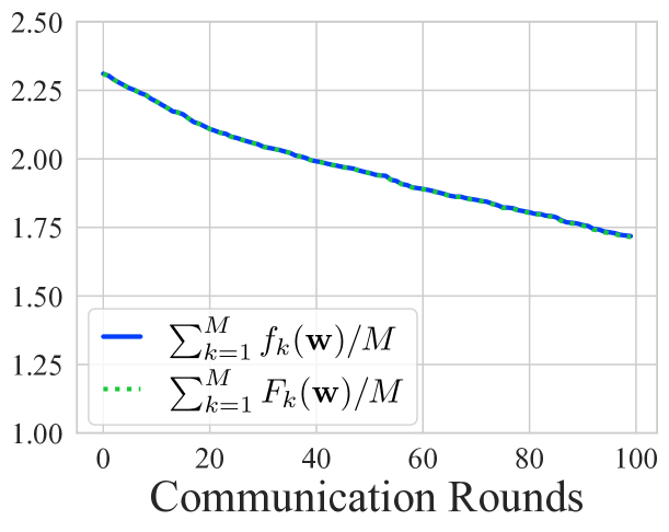
(a) FMNIST

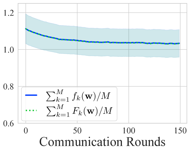
(b) Sent140

Figure 7: Comparison of the average of the true local losses across all clients ($\textstyle{\sum\nolimits_{k=1}^{M}f_{k}(\mathbf{w})/M}$) and the empirical local losses across all clients ($\textstyle{\sum\nolimits_{k=1}^{M}F_{k}(\mathbf{w})/M}$) where the former is calculated on the test dataset and the latter is calculated on the training dataset for the global model $\mathbf{w}$. We show that the average of the true local losses is nearly identical to the average empirical local loss across all clients empirically validating our relaxation of replacing $f_{k}(\mathbf{w})$ with $F_{k}(\mathbf{w})$.

Ablation Study on the Number of Local Steps $\tau_{l}$ to train $\widehat{\mathbf{w}}_{k},k\in[M]$.

We conduct an additional ablation study where we vary the number of local steps to obtain $\widehat{\mathbf{w}}_{k},k\in[M]$ for clients as shown in Table 4. Despite that a smaller number of local steps can lead to underfitting and a larger number of local steps can lead to overfitting, we show that all methods’ GM-Appeals do not vary much by the different number of local steps used for training.

	GM-Appeal			Preferred-Model Test Acc.
	$\tau_{l}=50$	$\tau_{l}=100$	$\tau_{l}=150$	$\tau_{l}=50$	$\tau_{l}=100$	$\tau_{l}=150$
FedAvg	$0.01\leavevmode\nobreak\ {\scriptstyle(\pm 0.01)}$	$0.01\leavevmode\nobreak\ {\scriptstyle(\pm 0.0)}$	$0.01\leavevmode\nobreak\ {\scriptstyle(\pm 0.0)}$	$98.56\leavevmode\nobreak\ {\scriptstyle(\pm 0.08)}$	$98.72\leavevmode\nobreak\ {\scriptstyle(\pm 1.02)}$	$98.75\leavevmode\nobreak\ {\scriptstyle(\pm 1.28)}$
FedProx	$0.01\leavevmode\nobreak\ {\scriptstyle(\pm 0.0)}$	$0.01\leavevmode\nobreak\ {\scriptstyle(\pm 0.0)}$	$0.01\leavevmode\nobreak\ {\scriptstyle(\pm 0.01)}$	$98.56\leavevmode\nobreak\ {\scriptstyle(\pm 1.15)}$	$98.72\leavevmode\nobreak\ {\scriptstyle(\pm 1.08)}$	$98.75\leavevmode\nobreak\ {\scriptstyle(\pm 1.05)}$
MaxFL	$\mathbf{0.55}\leavevmode\nobreak\ {\scriptstyle(\pm 0.0)}$	$\mathbf{0.55}\leavevmode\nobreak\ {\scriptstyle(\pm 0.0)}$	$\mathbf{0.55}\leavevmode\nobreak\ {\scriptstyle(\pm 0.0)}$	$\mathbf{98.64}\leavevmode\nobreak\ {\scriptstyle(\pm 1.03)}$	$98.77\leavevmode\nobreak\ {\scriptstyle(\pm 1.01)}$	$\mathbf{98.77}\leavevmode\nobreak\ {\scriptstyle(\pm 1.01)}$

Table 4: GM-Appeal and preferred-model test accuracy for MaxFL and different baselines with FMNIST for varying number of local steps $\tau_{l}$ to obtain $\widehat{\mathbf{w}}_{k},k\in[M]$ where $T=200$ is the total number of communication rounds for training the global model.

Preferred-model Test Accuracy for the Local-Tuning Results in Table 3.

In Table 3, we have shown how MaxFL can largely increase the GM-Appeal compared to the other baselines even when jointly used with local-tuning. In Table 5, we show the corresponding preferred-model test accuracies. We show that for the seen clients that were active during training, MaxFL achieves at least the same or higher preferred-model test accuracy than the other methods for all the different datasets. Hence, the clients are able to also gain from MaxFL by achieving the highest accuracy in average with their preferred models (either global model or solo-trained local model). For the unseen clients with FMNIST, FedProx achieves a slightly higher preferred-model test accuracy ($+0.05$) than MaxFL but with a much lower GM-Appeal of 0.46 (see Table 3) as MaxFL’s GM-Appeal is 0.56. For the other datasets with unseen clients, MaxFL achieves at least the same or higher preferred-model test accuracy than the other methods. This demonstrates that MaxFL consistently largely improves the GM-Appeal compared to the other methods while losing very little, if any, in terms of the preferred-model test accuracy.

	Seen Clients		Unseen Clients
	FMNIST	Sent140	FMNIST	Sent140
FedAvg	$99.37\leavevmode\nobreak\ {\scriptstyle(\pm 0.24)}$	$55.71\leavevmode\nobreak\ {\scriptstyle(\pm 0.46)}$	$99.50\leavevmode\nobreak\ {\scriptstyle(\pm 0.02)}$	$58.79\leavevmode\nobreak\ {\scriptstyle(\pm 0.67)}$
FedProx	$99.35\leavevmode\nobreak\ {\scriptstyle(\pm 0.23)}$	$55.75\leavevmode\nobreak\ {\scriptstyle(\pm 0.80)}$	$\mathbf{99.55}\leavevmode\nobreak\ {\scriptstyle(\pm 0.09)}$	$58.82\leavevmode\nobreak\ {\scriptstyle(\pm 0.72)}$
PerFedAvg	$99.20\leavevmode\nobreak\ {\scriptstyle(\pm 0.25)}$	$55.74\leavevmode\nobreak\ {\scriptstyle(\pm 0.80)}$	$98.98\leavevmode\nobreak\ {\scriptstyle(\pm 0.55)}$	$58.82\leavevmode\nobreak\ {\scriptstyle(\pm 0.72)}$
MW-Fed	$99.27\leavevmode\nobreak\ {\scriptstyle(\pm 0.39)}$	$55.06\leavevmode\nobreak\ {\scriptstyle(\pm 0.38)}$	$99.47\leavevmode\nobreak\ {\scriptstyle(\pm 0.08)}$	$57.36\leavevmode\nobreak\ {\scriptstyle(\pm 0.71)}$
MaxFL	$\mathbf{99.40}\leavevmode\nobreak\ {\scriptstyle(\pm 0.30)}$	$\mathbf{55.82}\leavevmode\nobreak\ {\scriptstyle(\pm 0.82)}$	$99.50\leavevmode\nobreak\ {\scriptstyle(\pm 0.02)}$	$\mathbf{58.88}\leavevmode\nobreak\ {\scriptstyle(\pm 0.77)}$

Table 5: Preferred-model test accuracy with the locally-tuned models with 5 local steps from the final global model for seen clients’ and unseen clients’ test data (the corresponding GM-Appeal is in Table 3).

	GM-Appeal		Preferred-Model Test Acc.
	FMNIST	Sent140	FMNIST	Sent140
q-FFL ($q=1$)	$0.03\leavevmode\nobreak\ {\scriptstyle(\pm 0.01)}$	$0.09\leavevmode\nobreak\ {\scriptstyle(\pm 0.06)}$	$99.24\leavevmode\nobreak\ {\scriptstyle(\pm 0.05)}$	$53.10\leavevmode\nobreak\ {\scriptstyle(\pm 2.63)}$
q-FFL ($q=10$)	$0.0\leavevmode\nobreak\ {\scriptstyle(\pm 0.0)}$	$0.09\leavevmode\nobreak\ {\scriptstyle(\pm 0.0)}$	$98.90\leavevmode\nobreak\ {\scriptstyle(\pm 0.01)}$	$52.71\leavevmode\nobreak\ {\scriptstyle(\pm 1.40)}$
MaxFL	$\mathbf{0.55}\leavevmode\nobreak\ {\scriptstyle(\pm 0.0)}$	$\mathbf{0.41}\leavevmode\nobreak\ {\scriptstyle(\pm 0.07)}$	$\mathbf{99.29}\leavevmode\nobreak\ {\scriptstyle(\pm 0.03)}$	$\mathbf{53.93}\leavevmode\nobreak\ {\scriptstyle(\pm 1.87)}$

Table 6: GM-Appeal and preferred-model test accuracy for the seen clients’ test data with the final global models trained via MaxFL and q-FFL [27] which aims in improving fairness. The baseline q-FFL with large $q$, e.g. $q=10$, emulates the behavior of another well-known algorithm for improving fairness named AFL [28].

Comparison with Algorithms for Fairness

Fair FL methods [27, 28] aim in training a global model that yields small variance across the clients’ test accuracies. These methods may satisfy the worst performing clients, but potentially at the cost of causing dissatisfaction from the best performing clients. We show in Table 6 that the common fair FL methods are indeed not effective in improving the overall clients’ GM-Appeal. We see that the fair FL methods achieve a GM-Appeal lower than 0.01 for all datasets while MaxFL achieves at least 0.40 for all datasets. Moreover, the preferred-model test accuracy is also higher for MaxFL compared to the fair FL methods. This underwelming performance of fair FL methods in GM-Appeal can be due to the fact that fair FL methods try to find the global model that performs well, in overall, over all clients which results in failing to satisfy any client.

Ablation Study on $f_{k}(\mathbf{w})\approx F_{k}(\mathbf{w})$.

One of the two key relaxations we use for MaxFL (see Section 2.2) is that we replace $f_{k}(\mathbf{w})-f_{k}(\widehat{\mathbf{w}}_{k})$ with $F_{k}(\mathbf{w})-F_{k}(\widehat{\mathbf{w}}_{k})$. In other words, we replace the true loss $f_{k}(\mathbf{w})=\mathbb{E}_{\xi\sim\mathcal{D}_{k}}[\ell(\mathbf{w},\xi)]$ with the empirical loss $F_{k}(\mathbf{w})=\frac{1}{|\mathcal{B}_{k}|}\sum_{\xi\in\mathcal{B}_{k}}\ell(\mathbf{w},\xi)$ for all clients $k\in[M]$. We have used the likely conjecture that the global model $\mathbf{w}$ is trained on the data of all clients, making it unlikely to overfit to the local data of any particular client, leading to $f_{k}(\mathbf{w})\approx F_{k}(\mathbf{w})$. We show in Fig. 7 that this is indeed the case. For all DNN experiments, we show that the average true local loss across all clients, i.e., $\textstyle{\sum\nolimits_{k=1}^{M}f_{k}(\mathbf{w})/M}$ is nearly identical to the average empirical local loss across all clients, i.e., $\textstyle{\sum\nolimits_{k=1}^{M}F_{k}(\mathbf{w})/M}$ given the training of the global model $\mathbf{w}$ throughout the communication rounds. This empirically validates our relaxation of the true local losses to the empirical local losses.

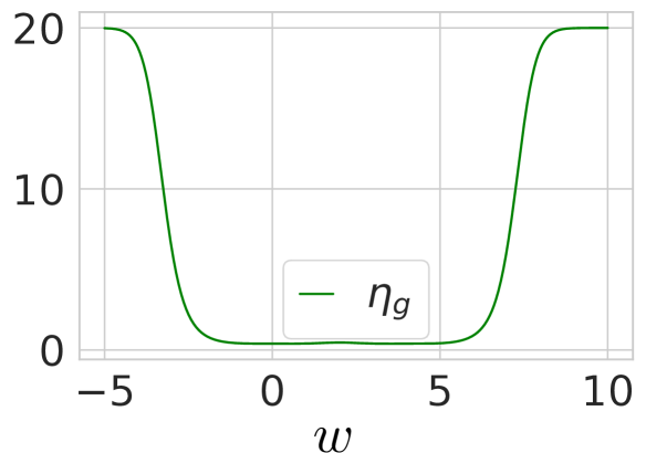
Figure 8: Behavior of Theoretical Learning Rate of MaxFL for the mean estimation example in Fig. 1(b). As expected from the theoretical learning rate formula, we see a higher learning rate in regions where the function is flat.

MaxFL’s Theoretical Learning Rate Behavior for Fig. 1 (b). Here, we provide a plot of MaxFL’s theoretical learning rate for the mean estimation example in Fig. 1(b) in Fig. 8 to show how the learning rate changes for different regions of the model. We show this plot as a proof of concept on the adaptive learning rate we discuss in Section 4. For the sigmoid function which is used for our MaxFL objective, using a global notion of smoothness can cause gradient descent to be too slow since global smoothness is determined by behavior at $w=0$ where $w$ is the model. In this case, it is better to use a local estimate of smoothness in the flat regions where $|w|>>0$. Recall that $\nabla^{2}\sigma(w)=\sigma(w)(1-\sigma(w))(1-2\sigma(w))<\sigma(x)(1-\sigma(w))$ and therefore setting the learning rate proportional to $\frac{1}{\sigma(w)(1-\sigma(w))}$ can increase the learning rate in flat regions where $\sigma(w)$ is close to 1 or 0. Following a similar argument, we can show that the learning rate in our objective should be proportional to $1/\left(\sum_{i=1}^{M}\sigma(F_{i}(w)-F_{i}(\hat{w}^{*})(1-\sigma(F_{i}(w)-F_{i}(\hat{w}^{*}))\right)$.

References

- [1] H. Brendan McMahan, Eider Moore, Daniel Ramage, Seth Hampson, and Blaise Agøura y Arcas. Communication-Efficient Learning of Deep Networks from Decentralized Data. International Conference on Artificial Intelligenece and Statistics (AISTATS), April 2017.
- [2] Peter Kairouz, H. Brendan McMahan, Brendan Avent, Aurelien Bellet, Mehdi Bennis, Arjun Nitin Bhagoji, Keith Bonawitz, Zachary Charles, Graham Cormode, Rachel Cummings, Rafael G. L. D’Oliveira, Salim El Rouayheb, David Evans, Josh Gardner, Zachary Garrett, Adria Gascon, Badih Ghazi, Phillip B. Gibbons, Marco Gruteser, Zaid Harchaoui, Chaoyang He, Lie He, Zhouyuan Huo, Ben Hutchinson, Justin Hsu, Martin Jaggi, Tara Javidi, Gauri Joshi, Mikhail Khodak, Jakub Konecny, Aleksandra Korolova, Farinaz Koushanfar, Sanmi Koyejo, Tancrede Lepoint, Yang Liu, Prateek Mittal, Mehryar Mohri, Richard Nock, Ayfer Ozgur, Rasmus Pagh, Mariana Raykova, Hang Qi, Daniel Ramage, Ramesh Raskar, Dawn Song, Weikang Song, Sebastian U. Stich, Ziteng Sun, Ananda Theertha Suresh, Florian Tramer, Praneeth Vepakomma, Jianyu Wang, Li Xiong, Zheng Xu, Qiang Yang, Felix X. Yu, Han Yu, and Sen Zhao. Advances and open problems in federated learning. arXiv preprint arXiv:1912.04977, 2019.
- [3] Tao Yu, Eugene Bagdasaryan, and Vitaly Shmatikov. Salvaging federated learning by local adaptation. arXiv preprint arXiv:2002.04758, 2020.
- [4] H Brendan McMahan, Daniel Ramage, Kunal Talwar, and Li Zhang. Learning differentially private recurrent language models. International Conference on Learning Representations, 2018.
- [5] Tan T. Nguyen and Scott Sanner. Algorithms for direct 0–1 loss optimization in binary classification. In Proceedings of the 30th International Conference on Machine Learning, volume 28, 2013.
- [6] Hamed Masnadi-shirazi and Nuno Vasconcelos. On the design of loss functions for classification: theory, robustness to outliers, and savageboost. In Advances in Neural Information Processing Systems(NIPS), 2008.
- [7] Jianyu Wang, Zachary Charles, Zheng Xu, Gauri Joshi, H Brendan McMahan, Maruan Al-Shedivat, Galen Andrew, Salman Avestimehr, Katharine Daly, Deepesh Data, et al. A field guide to federated optimization. arXiv preprint arXiv:2107.06917, 2021.
- [8] Sebastian U Stich. Local SGD converges fast and communicates little. In International Conference on Learning Representations (ICLR), 2019.
- [9] Sai Praneeth Karimireddy, Satyen Kale, Mehryar Mohri, Sashank J Reddi, Sebastian U Stich, and Ananda Theertha Suresh. SCAFFOLD: Stochastic controlled averaging for on-device federated learning. arXiv preprint arXiv:1910.06378, 2019.
- [10] I. Bistritz, A. J. Mann, and N. Bambos. Distributed distillation for on-device learning. In Advances in Neural Information Processing Systems, 2020.
- [11] Jianyu Wang, Qinghua Liu, Hao Liang, Gauri Joshi, and H. Vincent Poor. Tackling the Objective Inconsistency Problem in Heterogeneous Federated Optimization. preprint, May 2020.
- [12] Shai Shalev-Shwartz, Ohad Shamir, Nathan Srebro, and Karthik Sridharan. Stochastic convex optimization. In COLT, 2009.
- [13] Erlend S. Riis, Matthias J. Ehrhardt, G. R. W. Quispel, and Carola-Bibiane Schönlieb. A geometric integration approach to nonsmooth, nonconvex optimisation. Foundations of Computational Mathematics, 2021.
- [14] Kate Donahue and Jon Kleinberg. Model-sharing games: Analyzing federated learning under voluntary participation. In The Thirty-Fifth AAAI Conference on Artificial Intelligence (AAAI-21), 2021.
- [15] Kate Donahue and Jon Kleinberg. Optimality and stability in federated learning: A game-theoretic approach. In Advances in Neural Information Processing Systems, 2021.
- [16] Avrim Blum, Nika Haghtalab, Richard Lanas Phillips, and Han Shao. One for one, or all for all: Equilibria and optimality of collaboration in federated learning. In International Conference on Machine Learning, 2021.
- [17] Heqiang Wang and Jie Xu. Friends to help: Saving federated learning from client dropout. arXiv preprint arXiv:2205.13222, 2022.
- [18] Xinran Gu, Kaixuan Huang, Jingzhao Zhang, and Longbo Huang. Fast federated learning in the presence of arbitrary device unavailability. Advances in Neural Information Processing Systems, 34:12052–12064, 2021.
- [19] Jingoo Han, Ahmad Faraz Khan, Syed Zawad, Ali Anwar, Nathalie Baracaldo Angel, Yi Zhou, Feng Yan, and Ali R. Butt. Tokenized incentive for federated learning. In Proceedings of the Federated Learning Workshop at the Association for the Advancement of Artificial Intelligence (AAAI) Conference, 2022.
- [20] Jiawen Kang, Zehui Xiong, Dusit Niyato, Han Yu, Ying-Chang Liang, and Dong In Kim. Incentive design for efficient federated learning in mobile networks: A contract theory approach. In 2019 IEEE VTS Asia Pacific Wireless Communications Symposium (APWCS), pages 1–5, 2019.
- [21] Meng Zhang, Ermin Wei, and Randall Berry. Faithful edge federated learning: Scalability and privacy. IEEE Journal on Selected Areas in Communications, 39(12):3790–3804, 2021.
- [22] Virginia Smith, Chao-Kai Chiang, Maziar Sanjabi, and Ameet S Talwalkar. Federated multi-task learning. In Advances in Neural Information Processing Systems, pages 4424–4434. 2017.
- [23] Canh T. Dinh, Nguten H. Tran, and Tuan Dung Nguyen. Personalized federated learning with moreau envelopes. In Advances in Neural Information Processing Systems, 2020.
- [24] Alireza Fallah, Aryan Mokhtari, and Asuman Ozdaglar. Personalized federated learning with theoretical guarantees: A model-agnostic meta-learning approach. In Advances in Neural Information Processing Systems, 2020.
- [25] Tian Li, Shengyuan Hu, Ahmad Beirami, and Virginia Smith. Ditto: Fair and robust federated learning through personalization. In Proceedings of the 38th International Conference on Machine Learning, 2021.
- [26] Yihan Jiang, Jakub Konecny, Keith Rush, and Sreeram Kannan. Improving federated learning personalization via model agnostic meta learning. arXiv 1909.12488, 2019.
- [27] Tian Li, Maziar Sanjabi, and Virginia Smith. Fair resource allocation in federated learning. arXiv preprint arXiv:1905.10497, 2019.
- [28] Mehryar Mohri, Gary Sivek, and Ananda Theertha Suresh. Agnostic federated learning. In Kamalika Chaudhuri and Ruslan Salakhutdinov, editors, Proceedings of the 36th International Conference on Machine Learning, volume 97 of Proceedings of Machine Learning Research, pages 4615–4625, Long Beach, California, USA, 09–15 Jun 2019. PMLR.
- [29] Han Xiao, Kashif Rasul, and Roland Vollgraf. Fashion-mnist: a novel image dataset for benchmarking machine learning algorithms. https://arxiv.org/abs/1708.07747, aug 2017.
- [30] Gregory Cohen, Saeed Afshar, Jonathan Tapson, and André van Schaik. EMNIST: an extension of MNIST to handwritten letters. arXiv preprint arXiv:1702.05373, 2017.
- [31] Alec Go, Richa Bhayani, and Lei Huang. Twitter sentiment classification using distant supervision. CS224N Project Report, Stanford, 2009.
- [32] Anit Kumar Sahu, Tian Li, Maziar Sanjabi, Manzil Zaheer, Ameet Talwalkar, and Virginia Smith. Federated optimization for heterogeneous networks. In Proceedings of the 3rd MLSys Conference, January 2020.
- [33] Yûsaku Komatu. Elementary inequalities for mills’ ratio. Reports of Statistical Application Research (Union of Japanese Scientific Engineers), 4:69–70, 1955.
- [34] Divyansh Jhunjhunwala, Pranay Sharma, Aushim Nagarkatti, and Gauri Joshi. Fedvarp: Tackling the variance due to partial client participation in federated learning. arXiv, 2022.
- [35] Charles R. Harris, K. Jarrod Millman, Stéfan J. van der Walt, Ralf Gommers, Pauli Virtanen, David Cournapeau, Eric Wieser, Julian Taylor, Sebastian Berg, Nathaniel J. Smith, Robert Kern, Matti Picus, Stephan Hoyer, Marten H. van Kerkwijk, Matthew Brett, Allan Haldane, Jaime Fernández del Río, Mark Wiebe, Pearu Peterson, Pierre Gérard-Marchant, Kevin Sheppard, Tyler Reddy, Warren Weckesser, Hameer Abbasi, Christoph Gohlke, and Travis E. Oliphant. Array programming with NumPy. Nature, 585(7825):357–362, September 2020.
- [36] Pauli Virtanen, Ralf Gommers, Travis E Oliphant, Matt Haberland, Tyler Reddy, David Cournapeau, Evgeni Burovski, Pearu Peterson, Warren Weckesser, Jonathan Bright, et al. Scipy 1.0: fundamental algorithms for scientific computing in python. Nature methods, 17(3):261–272, 2020.
- [37] Tzu-Ming Harry Hsu, Hang Qi, and Matthew Brown. Measuring the effects of non-identical data distribution for federated visual classification. In International Workshop on Federated Learning for User Privacy and Data Confidentiality in Conjunction with NeurIPS 2019 (FL-NeurIPS’19), December 2019.
- [38] Jeffrey Pennington, Richard Socher, and Christopher D. Manning. Glove: Global vectors for word representation. In Empirical Methods in Natural Language Processing (EMNLP), pages 1532–1543, 2014.