Bound orbits around charged black strings

Abstract

We study the geodesics of $5d$ Reissner-Nordstrom and nonsingular black strings, and establish a rational bound orbit taxonomy for both massive as well as null test particles. For the timelike case, test particles with high energy (that would have made them plunge into or scatter off a black hole) could still form bound orbits around the black strings. We calculate the accumulated angles of the corresponding radial periods and show that they are higher than their $4d$ counterparts. For the null case, we found the existence of stable null orbits outside their respective horizons, which do not exist in the four dimensions except at their extremal limit.

I Introduction

Black holes in higher dimensions have long been an interesting as well as intriguing subject. Mathematically, the additions of extra dimensions pose a considerable challenge to obtaining exact solutions. Astrophysically, their signature might shed light on the unification of fundamental forces. Although the possibility of extra dimension has been considered by Kaluza and Klein as early as the 1920s Kaluza:1921tu , it was Tangherlini who generalized the Reissner-Nordstrom (RN) black hole to higher dimensions Tangherlini:1963bw . Myers and Perry then followed in obtaining solutions for higher-dimensional Kerr-Newman Myers:1986un . The spherical event horizon is not the only possible higher-dimensional BH solution. A trivial extension of a Schwarzschild black hole to a higher dimension would be a charged black string whose metric does not depend on its compact extra dimension. Such solution has been shown to be stable by Gregory and Laflamme Gregory:1987nb . More nontrivial black strings are, of course, abundant in the literature Gibbons:1987ps ; Gregory:1995qh ; Emparan:2001wn .

Even in $4d$ due to its very definition, a black hole cannot be observed directly. Thus, so far the probe for their existence relies on: (i) the gravitational wave LIGOScientific:2016aoc and (ii) orbital dynamics around it (e.g., perihelion precession GRAVITY:2020gka , gravitational lensing and shadow EventHorizonTelescope:2019dse ; Akiyama2022 , or photon orbits GRAVITY:2018 ). It was Hagihara in 1930 that first obtained the exact solution tof the Schwarzschild geodesic Hagihara(1930) (see also Hackmann Hackmann:2010tqa ). The analytic solution is in the form of the Weierstrass elliptic function. It was later extended to the case of (static and rotating) black strings by Grunau Grunau:2013oca . The behavior of massive neutral and charged particles around weekly magnetized Schwarzschild string was studied Rezvanjou:2017hox .

In a series of interesting papers, Levin and collaborators propose a taxonomy based on isomorphism between periodic orbits around (or of pairs of) $4d$ black holes and rational numbers Levin:2008mq ; Levin:2008ci ; Perez-Giz:2008ajn ; Healy:2009zm . They found that there exists a set of three integers $(z,w,v)$ that can be combined to form a rational number

$$q\equiv w+{v\over z},$$ (1)

that completely parametrizes every (timelike or null) bound orbit. Here $w$ defines the number of whirls, $z$ expresses the number of leaves, and $v$ denotes the order the leaves are traced out. Within this formalism, precession of Mercury’s perihelion can be perceived as periodic orbit with very large $z$, around $z\sim 1.296\times 10^{7}$ Levin:2008mq . This rational orbit formalism has been applied to Schwarzchild, RN Misra:2010pu , and Kerr solutions Levin:2008mq , as well to the black hole binary system.

Even though its unchraged geodesic has extensively been studied Grunau:2013oca , to the best of our knowledge no one yet elaborates the rational orbit formalism on the charged black string. It is therefore the purpose of this paper to accomplish this task. Since the orbital motion is confined to $4d$, the hope is that the effect of one extra spatial dimension will give distinct observational signatures that can distinguish black hole from black string. The “anomaly” orbital motion around a black object can thus serve as an astrophysical probe for the existence of extra dimension. To do so, we specifically study two types of charged strings: the charged Gregory-Laflamme Gregory:1987nb and the nonsingular black strings. The latter is the $5d$ extension of the well-known Bardeen black hole bardeen . These two are simple toy models but at the same time are rich enough to prove our point. The organization is as follows. We examine the general black string geodesic and effective potential in Section II. Section III is devoted to the all possible types of orbits and the formalism of rational orbit taxonomy. The orbital zoo of RN and Bardeen black strings are presented in Sections IV and  V, respectively. Finally, we conclude the result of this study in VI.

II Black String Geodesics

A trivial $5d$ extension of a static and spherically-symmetric black hole can always be written as Gregory:1987nb

$$ds^{2}=-f(r)dt^{2}+f(r)^{-1}dr^{2}+r^{2}d\Omega^{2}+d\omega^{2},$$ (2)

where $\omega$ is an extra compact spatial dimension and $f(r)$ is any metric solution that solves the $5d$ Einstein equations. Since the string preserves the $4d$ spherical symmetry, under the condition of equatorial plane ($\theta=\pi/2$) the invariance condition $g_{\mu\nu}\dot{x}^{\mu}\dot{x}^{\nu}=-\epsilon$ gives the constraint equation as

$$-\epsilon=-f(r)\dot{t}^{2}+f(r)^{-1}\dot{r}^{2}+r^{2}\dot{\phi}^{2}+\dot{\omega}^{2},$$ (3)

where $\epsilon=\{1,0\}$ corresponds to timelike and null geodesics, respectively. Using Euler-Lagrange equation, we obtain the equation of motion for each coordinate:

$$\dot{t} = \frac{dt}{d\tau}=\frac{\mathbb{E}}{f(r)},$$

$$\dot{\phi} = \frac{d\phi}{d\tau}=\frac{\mathbb{L}}{r^{2}},$$

$$\dot{\omega} = \frac{d\omega}{d\tau}=\mathbb{J}.$$ (4)

Inserting (II) into (3) and rescaling $\mathbb{L}^{2}\rightarrow 1/L$, $\mathbb{J}^{2}\rightarrow J$, we have the geodesic equation in the form of

$$\dot{r}^{2}=\mathbb{E}^{2}-V_{eff},$$ (5)

where the effective potential $V_{eff}$ can be written as

$$V_{eff}(r) = f(r)\left(\epsilon+J+\frac{1}{Lr^{2}}\right).$$ (6)

III Black String Orbits

III.1 Types of Orbit

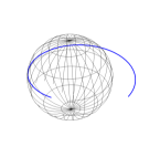
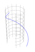
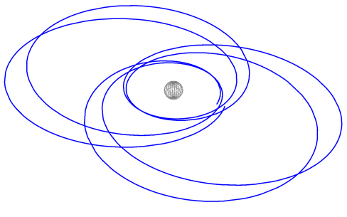
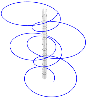
Figure 1: Typicals of terminating orbit, escape orbit, and bound orbit around black hole (left column) and black ring (right columnn).

Particle trajectories in black string can be classified in terms of orbital types and regions. Denoting $r_{EH}$ as the radius of outer event horizon, the three possible orbit types and their definitions are listed as below, in which their visualizations are shown in Fig. 1. Here we use similar convention as in Grunau Grunau:2013oca .

1. Terminating orbit (TO): particles arrive at a periapsis $r_{p}$ and falls into singularity.

2. Escape orbit (EO): particles come from $\infty$, approach a periapsis $r_{p}$, and return to $\infty$.

3. Bound orbit (BO): particles oscillate between its periapsis and apoapsis under the condition of $r_{EH}<r_{p}<r_{a}<\infty$.

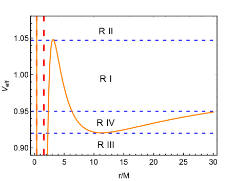
Figure 2: All possible regions (R I to R IV) according to various energy level. The blue line refers to energy level $\mathbb{E}^{2}$.

Region	Positive Real Zeros	Orbit Types
I	2	TO, EO
II	0	EO
III	1	TO
IV	3	TO, BO

Table 1: The classification of regions based on its effective $V_{eff}$ potential and particle energy level $E$ along with their corresponding possible orbit types.

Based on the effective potential, the regions can be classified using the Hackman formalism Hackmann:2010tqa . Solving the Eq. (5) results in various scenarios based on the numbers of its positive real solutions, which are shown in Table 1. To help understanding the regions better, the dependence of the orbits on the energy levels is shown in Fig. 2.

A typical $V_{eff}$ we study here generically have three turning points, as we shall see later, only two of which are outside the horizon. The local maxima represent the unstable circular orbit (UCO), while the local minima identify the stable circular orbit (SCO). Both circular orbits (CO) satisfy

$$\dot{r}^{2}=0,\ \ \ \partial_{r}V_{eff}=0,$$ (7)

which translates into

$$f(r_{CO})\left(J+\epsilon+{1\over Lr_{CO}^{2}}\right) = \mathbb{E}^{2},$$

$$f^{\prime}(r_{CO})\left(J+\epsilon+{1\over Lr_{CO}^{2}}\right)-{2f(r_{CO})\over Lr_{CO}^{3}} = 0.$$

Both CO depend on the angular momenta and black hole’s charge. For a given black hole there exists a critical circular radius beyond which it no longer supports bound orbits. For timelike case this critical value is called the innermost stable circular orbit (ISCO), and this is achieved when UCO and SCO radii merge. Mathematically, this is the inflection point of the effective potential,

$$V_{eff}=\mathbb{E}^{2},\ \ \ \partial_{r}V_{eff}=0,\ \ \ \partial^{2}_{r}V_{eff}=0.$$ (9)

This adds the following condition,

$$r\left[rf^{\prime\prime}(r)\left(Lr^{2}(J+\epsilon)+1\right)-4f^{\prime}(r)\right]+6f(r)=0,$$ (10)

into (III.1).

III.2 Overview of Rational Orbits Taxonomy

Here we briefly review the scheme of Levin and Perez-Giz in assigning each orbital solution to a distinct rational number Levin:2008mq . Any (positive) rational number can always be cast as

$$q=s+{m\over n},$$ (11)

where $s\geq 0$ is an integer and $1\leq m\leq n-1$ are (relatively) prime numbers. This taxonomy draws correspondence between $q$ and the topological features of orbit. The claim is that each periodic orbit is completely characterized by three integers $(z,w,v)$ that can be expressed as rational number, Eq. 1. Each of them corresponds to a specific topological trait of a periodic orbit. The first and most tangible number is $z$, which is the number of leaves (or ”zooms”) of the orbit. The second integer, $w$, is the number of whirls which the particle performs in its path from apastron to periastron to the next apastron. Note that every particle performs at least a full $2\pi$ trip. The number of whirls is the additional integer number of full $2\pi$ accomplished beyond this. The last number $v$, the vertex number, differentiate between orbits that have equal $z$ and $w$ but are geometrically distinct. Particle can skip leaves in its motion from apastron to apastron. One important thing to address is the degeneracy that arises when the quotient $v=z$ is a reducible fraction. This is solved by requiring $v$ and $z$ to be relatively prime. The bounds on v then can be written as

$$1\leq v\leq z-1\,\,\,\, \text{if}\,\,\,\,\,\,\,\,z>1\,\,\text{and}\,\,z,v\,\,\text{are relatively prime}$$ (12)

$$v=0\,\,\,\, \text{if}\,\,\,\,\,\,\,\,z=1.$$

The proof of such claim is based on the fact that for a periodic orbit, the accumulated angle between one apastron to another apastron can be expressed as

$$\Delta\varphi_{r}=2\pi\left(1+q\right)={\Delta\varphi\over z},$$ (13)

where $\Delta\varphi\equiv z\Delta\varphi_{r}$ is the total accumulated angle in a complete orbit. We may also define the radial period as the (affine) time taken by particle to return to the same radius upon starting at the apsis $r_{a}$ (where $\mathbb{E}^{2}=V_{eff}$) Levin:2009sk ; Babar:2017gsg . If within this period, the evolution of $\varphi$ is an integer multiple of $2\pi$, we have a periodic orbit. Therefore the accumulated radial angle can be written as

$$\Delta\varphi_{r}=2\int_{r_{p}}^{r_{a}}\frac{\dot{\phi}}{\dot{r}}dr=2\int_{r_{p}}^{r_{a}}\frac{dr}{Lr^{2}\sqrt{\mathbb{E}^{2}-f(r)\left(\epsilon+J+\frac{1}{Lr^{2}}\right)}},$$ (14)

where $r_{p}$ is the periastron radius. The rational number in Eq.(13) can be related to the orbital angular frequency by the following arguments. Every eccentric equatorial orbit has two types of frequencies: the radial ($\omega_{r}$) and angular ($\omega_{\varphi}$) frequencies. They are given by

$$\omega_{r} = {2\pi\over T_{r}},$$

$$\omega_{\varphi} = {1\over T_{r}}\int_{0}^{T_{r}}\frac{d\varphi}{dt}dt={\Delta\varphi_{r}\over T_{r}},$$ (15)

where $T_{r}$ is the period of one radial cycle. Any periodic orbit must then satisfy

$${\omega_{\varphi}\over\omega_{r}}={\Delta\varphi_{r}\over 2\pi}=1+q.$$ (16)

IV RN Black String

We consider the RN black string. It turns out that

$$f(r)=1-{2M\over r}+{Q^{2}\over r^{2}},$$ (17)

is still the solution of the corresponding $5d$ Einstein’s equations. Alternatively, we can perceive this metric as a solution arising from the Einstein-Maxwell compactification along the framework of Quasitopological Electromagnetism (QTE) theory Cisterna:2020rkc ; Cisterna:2021ckn . The horizons are still located at $r_{\pm}=M\pm\sqrt{M^{2}-Q^{2}}$, stretching to extra dimension and creating a hypercylindrical topology. Despite the remarkable simplicity in the metric solution, its geodesic phenomenology is not quite that trivial. There is a rich family of orbital solutions, both for timelike and null particles.

The typical $V_{eff}$ for massive particles is shown on Fig. 3. Notice that the local maximum rises along with the increase of $J$ value. Since energy and angular momentum are inversely proportional (see Eq. (5)), this means that the existence of bound orbit with bigger value of the constant $J$ requires test particles to have smaller $L$. For massless particles, the $V_{eff}$ is shown on Fig. 4. We observe the same trend as revealed in the timelike one. Nonetheless, we notice that in higher angular momentum case, the existence of additional dimension ($J>0$) elevate the potential and create a condition that allows photon to form bound orbits.

IV.1 Timelike CO and ISCO

The existence of CO and ISCO for timelike geodesic in $4d$ RN black hole has been widely discussed in Pugliese:2010ps ; Schroven:2020ltb and the references therein. As stated earlier, the condition for CO, given by Eq. (III.1), for the RN string translates into

$$\left(J-\mathbb{E}^{2}+1\right)Lr_{CO}^{4}-2(J+1)MLr_{CO}^{3}+\left[\left(J+1\right)LQ^{2}+1\right]r_{CO}^{2}-2Mr_{CO}+Q^{2} = 0,$$

$$2(J+1)MLr_{CO}^{3}-2\left[1-\left(J+1\right)LQ^{2}\right]r_{CO}^{2}+6Mr_{CO}-4Q^{2} = 0,$$

where $r_{CO}$ is the circular radii. Simple algebra shows that those equations can be solved simultaneously to obtain one-parameter class of solutions parametrized by $r_{CO}$,

$$L = \frac{3Mr_{CO}-2Q^{2}-r_{CO}^{2}}{(J+1)r_{CO}^{2}\left(Q^{2}-Mr_{CO}\right)},$$

$$\mathbb{E}^{2} = \frac{(J+1)\left(-2Mr_{CO}+Q^{2}+r_{CO}^{2}\right)^{2}}{r_{CO}^{2}\left(-3Mr_{CO}+2Q^{2}+r_{CO}^{2}\right)}.$$

In the extremal case we have

$$L={r-2M\over\left(1+J\right)Mr^{2}},\ \ \ \mathbb{E}^{2}={\left(1+J\right)\left(r-M\right)^{3}\over\left(r-2M\right)r^{2}}.$$ (20)

When $J\rightarrow 0$ they reduce to the circular motion conditions for neutral test particles around $4d$ RN black hole Pugliese:2010ps .

For any given $L$ the ISCO is the smallest radius of circular orbit before the particle plunges into the black hole. It is the inflection point of $V_{eff}$. From condition (9), the additional equation to be solved is

$$4(J+1)LMr_{ISCO}^{3}-6\left[(J+1)LQ^{2}+1\right]r_{ISCO}^{2}+24Mr_{ISCO}-20Q^{2}=0.$$ (21)

Since the extra-dimensional signature always appears multiplying $L$, i.e., $(1+J)L$, then from the expression of $L$ in (IV.1) it is obvious that the ISCO radii satisfy

$$Mr_{ISCO}^{3}-6M^{2}r_{ISCO}^{2}+9MQ^{2}r_{ISCO}-4Q^{4}=0.$$ (22)

The same thing happens for the extremal black strings. The ISCO radii becomes

$$r_{ISCO}^{2}-5Mr_{ISCO}+4M^{2}=0,$$ (23)

with solutions

$$r_{ISCO}=\{M,\ 4M\},$$ (24)

the same as the extremal $4d$ RN ISCO; the timelike ISCO is oblivion to the existence of extra dimension (i.e., independent of $J$). Notice that this is precisely the same condition for ISCO in $4d$ RN black hole Pugliese:2010ps .

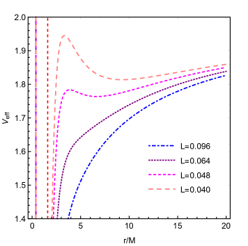
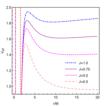
Figure 3: [Left] Plot of effective potential for massive particles in RN two-horizon case with $Q=0.8$ and $J=1$ and various values of $L$ and [Right] similar plot with $L=0.04$ and various values of $J$. The dashed red lines refer to the inner and outer horizons.

IV.2 Null Circular Orbit

For null geodesic ($\epsilon=0$) it is customary to define impact parameter $b$, where $b^{2}\equiv 1/\mathbb{E}^{2}L$. The geodesic equation (5) becomes

$$\dot{r}^{2}+V_{eff}=b^{2},\ \ \ V_{eff}\equiv f(r)\left(j+{1\over r^{2}}\right),$$ (25)

where $j\equiv JL$ and we subsequently rescale the proper time $\tau\rightarrow\tau/L$. It is well-known that $4d$ RN spacetime does not support stable CO, except in the extremal limit. To be precise, for any given charge $Q/M$ the $\partial_{r}V_{eff}=0$ condition for null gives us a quadratic equation whose roots are

$$r^{\pm}_{CO}={3M\pm\sqrt{9M^{2}-8Q^{2}}\over 2}.$$ (26)

One can easily observe that $r^{-}_{CO}$ is at the local minima of $V_{eff}$ and is between the two horizons. Thus, the only observable CO, called the photon sphere, $r^{+}_{CO}$ is unstable Pradhan:2010ws ; Khoo:2016xqv . At $M=Q$, the CO radii shifts further into

$$r^{\pm}_{CO}=\{2M,\ M\};$$ (27)

the stable $r_{CO}$ coincides with the extremal horizon $r_{extr}$.

The situation is rather different in this $5d$ black string. The additional term that multiplies $j$ in $V_{eff}$ gives qubic equation for the $\partial_{r}V_{eff}=0$,

$$jMr_{CO}^{3}-\left(jQ^{2}+1\right)r_{CO}^{2}+3Mr_{CO}-2Q^{2}=0,$$ (28)

i.e., in general we have an additional local minima of $V_{eff}$. By adjusting $j$ we can have a stable photon sphere outside the outer horizon, $r_{ps}>r_{+}$. For extremal case, Eq. (28) has three roots

$$r_{CO}^{e,\pm}=\bigg{\{}M,\ {1\pm\sqrt{1-8jM^{2}}\over 2jM}\bigg{\}},$$ (29)

one of which lies on the extremal horizon, $r^{e}_{CO}=r_{extr}=M$. The other two ($r_{\pm}$) are real and located outside $r_{extr}$ provided the following condition is satisfied,

$$0<j<{1\over 8M^{2}}.$$ (30)

The $r_{CO}^{+}$ ($r_{CO}^{-}$) act as the stable (unstable) radii. As $j\rightarrow 0$ we have $r_{CO}^{\pm}\rightarrow\{2M,\infty\}$ and we recover the condition (27).

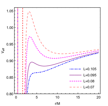
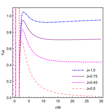
Figure 4: [Left] Plot of effective potential for light particles in RN two-horizon case with $Q=0.8$ and $J=1$ and various values of $L$ and [Right] similar plot with $L=0.07$ and various values of $J$. The dashed red lines refer to the inner and outer horizons.

IV.3 Exact Solutions of the Geodesic

Studying the shape of $V_{eff}$ can only tell us to so much about the qualitative types of orbits. To know their specific shapes we must solve the geodesic equation. Using the black string metric above and setting $r=r(\phi)$, the geodesic equation (5) can be cast into

$$\bigg{(}\frac{dr}{d\phi}\bigg{)}^{2}=\mathbb{E}^{2}Lr^{4}-f(r)\left(r^{2}+Lr^{4}(J+\epsilon)\right)\equiv\mathcal{R}(r).$$ (31)

This can be simplified by rescaling $r\rightarrow r/M$, $Q\rightarrow Q/M$, $L\rightarrow L/M^{2}$, and defining:
$v\equiv L(\mathbb{E}^{2}-(J+\epsilon)),\ w\equiv 2L(J+\epsilon),\ x\equiv-LQ^{2}(J+\epsilon)-1,\ y\equiv 2,$ and $z\equiv-Q^{2},$ such that Eq. (31) now reads

$$\bigg{(}\frac{dr}{d\phi}\bigg{)}^{2}=vr^{4}+wr^{3}+xr^{2}+yr+z.$$ (32)

Further simplification by expanding $r$ around (one of its zeros) $r=s+r_{0}$ and defining: $a_{0}\equiv v,\ a_{1}\equiv 4r_{0}v+w,\ a_{2}\equiv 6r_{0}^{2}v+3r_{0}w+x,$ and $a_{3}\equiv 4r_{0}^{3}v+3r_{0}^{2}w+2r_{0}x+y$, transform Eq. (32) into

$$\bigg{(}\frac{ds}{d\phi}\bigg{)}^{2}=a_{0}s^{4}+a_{1}s^{3}+a_{2}s^{2}+a_{3}s.$$ (33)

The degree of the corresponding polynomial can be reduced by setting $r\equiv 1/u$, and further by $u\equiv 4y/a_{3}-a_{2}/3a_{3}$. We then obtain the Weierstrass form

$$\bigg{(}\frac{dy}{d\phi}\bigg{)}^{2}=4y^{3}-g_{2}y-g_{3},$$ (34)

where $g_{2}$ and $g_{3}$ are given as

$$g_{2} = \frac{1}{16}\left(\frac{4a_{2}^{2}}{3}-4a_{1}a_{3}\right),$$ (35)

$$g_{3} = \frac{1}{16}\left(\frac{1}{3}a_{1}a_{3}a_{2}-\frac{1}{27}2a_{2}^{3}-a_{0}a_{3}^{2}\right).$$ (36)

Eq. (31) admits analytical solution in terms of Weierstrass $\wp$-function Hackmann:2010tqa :

$$r(\phi)=r_{0}+\frac{3a_{3}}{12\wp(\phi-\phi_{in})-a_{2}}$$ (37)

where the initial angle $\phi_{in}$ is only dependent on $\phi_{0}$ and $y_{0}$:

$$\phi_{in}=\phi_{0}+\int_{y_{0}}^{\infty}\frac{dy}{\sqrt{4y^{3}-g_{2}y-g_{3}}},\,\,\ \ \ \ y_{0}\equiv\frac{1}{4}\bigg{(}\frac{a_{3}}{r_{in}-r_{0}}+\frac{a_{2}}{3}\bigg{)}.$$ (38)

Making use of (II) we have the equation for $\omega$ as

$$\bigg{(}\frac{d\omega}{d\phi}\bigg{)}=J\sqrt{L}r(\phi)^{2},$$ (39)

which gives the solution of $\omega$ in terms of $\phi$ as

$$\omega=J\sqrt{L}\int_{\phi_{0}}^{\infty}r(\phi)^{2}d\phi.$$ (40)

Eq. (40) is later to play a significant role in enabling null bound orbit outside the string’s horizons.

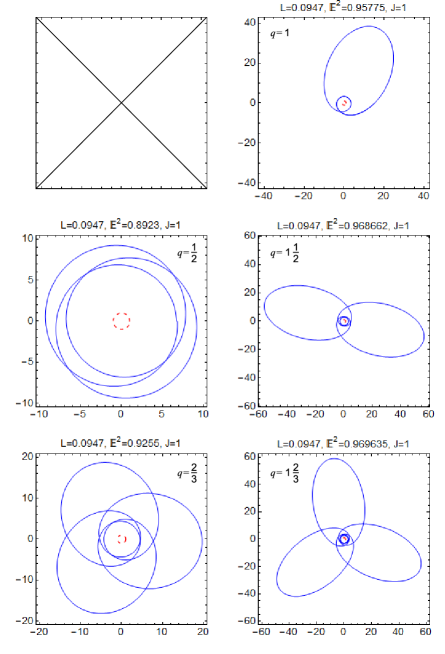
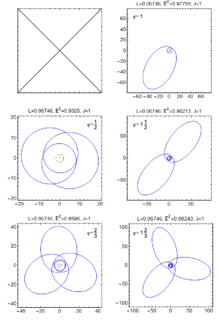
Figure 5: The $z=1,2,3$ orbits in RN null condition: extremal case with $w=0$ for the first column and $w=1$ for the second column; two-horizon case with $w=0$ for the third column and $w=1$ for the fourth column. Note that the first entries in the first and third column are blank because the $q=0+\frac{0}{1}$ orbits are inaccessible.

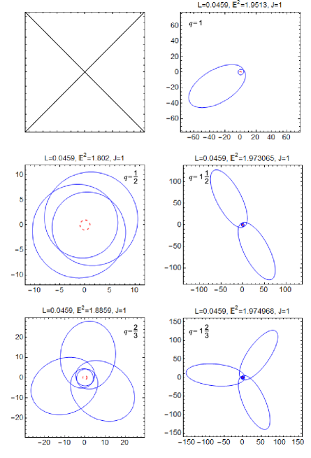
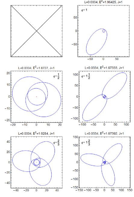
Figure 6: The $z=1,2,3$ orbits in RN timelike condition: extremal case with $w=0$ for the first column and $w=1$ for the second column; two-horizon case with $w=0$ for the third column and $w=1$ for the fourth column. Note that the first entries in the first and third column are blank because the $q=0+\frac{0}{1}$ orbits are inaccessible.

IV.4 RN Black String’s Bound Orbit Taxonomy

As discussed above, the black string’s $V_{eff}$ is quartic in $r$, so in general it gives three local extrema; an additional local minimum outside the horizon. In this work we limit ourselves only to the case of physical orbits; that is, which lies outside the horizon and can thus be observable. We avoid discussing the tricky case of horizon-crossing orbits despite the premise of many-world orbits by Grunau and Kagramanova, in which the orbit is viewed as infinite continuity of the patches of the spacetime Grunau:2010gd . Armed with the aforementioned taxonomy in III.2, we carefully examine the bounded domain of region IV (Fig. 2) in RN black string potential and present the periodic orbits up to 3 zooms and 2 whirls. The whole existence of stable null orbits in our case is genuine. The $J$-factor leads to the existence of periodic orbits, as opposed to the $4d$ case where no such stable orbits present Misra:2010pu ; Pradhan:2010ws . The plots are shown in Fig. 5.

$q$ SCO 1/2 2/3 1 1 1/2 1 2/3 UCO $\mathbb{E}$ (Extremal) Position 1.791566220 0.00% 1.802000000 5.62% 1.885900000 50.79% 1.951300000 86.00% 1.973065000 97.72% 1.974968000 98.75% 1.977293000 100.00% $\mathbb{E}$ (Two-horizon) Position 1.841640600 0.00% 1.872700000 23.38% 1.928400000 65.31% 1.964250000 92.30% 1.973330000 99.14% 1.973920000 99.58% 1.974477000 100.00% Deviation - 12.56% 10.27% 4.45% 1.00% 0.59% -

Table 2: Comparison of energy level and the position of particular orbit inside the energy range as percentage for timelike case in extremal and two-horizon RN black string. SCO refers to the bottom level of energy range (no whirl), while UCO refers to the top one (maximum whirl).

$q$ SCO 1/2 2/3 1 1 1/2 1 2/3 UCO $\mathbb{E}$ (Extremal) Position 0.891967985 0.00% 0.894300000 2.96% 0.925500000 42.51% 0.957750000 83.39% 0.968662000 97.22% 0.969635000 98.46% 0.970851807 100.00% $\mathbb{E}$ (Two-horizon) Position 0.919894000 0.00% 0.932500000 20.07% 0.959600000 63.20% 0.977550000 91.77% 0.982130000 99.06% 0.982430000 99.54% 0.982718600 100.00% Deviation - 12.10% 14.63% 5.93% 1.30% 0.77% -

Table 3: Comparison of energy level and the position of particular orbit inside the energy range as percentage for null case in extremal and two-horizon RN black string. SCO refers to the bottom level of energy range (no whirl), while UCO refers to the top one (maximum whirl).

Levin in Levin:2009sk shows that, since rational numbers are discrete so are the energy levels that produce the orbits. The existence of bound orbits are bounded by UCO and SCO, so we can quantify the level energy by the deviation from them. We define the corresponding deviation $\eta$ as

$$\eta\equiv{\left(\mathbb{E}-\mathbb{E}_{SCO}\right)\over\left(\mathbb{E}_{UCO}-\mathbb{E}_{SCO}\right)}\bigg{|}_{timelike/null}.$$ (41)

In Table 2 we list the energy level of various periodic orbits according to their energy level, for massive particles, in both extremal and two-horizon RN black string. Similar table for light particles is shown in Table 3. The table shows increasing number of rational number as it goes down the list. One behavior that is observed in both cases is the standard deviations, while fluctuate, tends to decrease as energy level rises to UCO. If we calculate the average of deviation for timelike and null condition, we obtain the value $6.36\%$ and $6.94\%$, respectively. The reasoning of why we separate the table by horizon case becomes clear when we pay attention to each deviation average: $2.03\%$ for extremal case and $0.86\%$ for two horizon one, which is way smaller than the numbers earlier. This finding means that the distance between energy levels is more consistent in each specific horizon case.

q	$\Delta\varphi_{r-4d}$	$\Delta\varphi_{r-5d}$
1/2	31.1018	44.0076
2/3	34.5575	48.8576
1	41.4694	58.634
1 1/2	51.8373	73.2913
1 2/3	48.085	78.1832

Table 4: Accumulated radial angle for extremal RN black holes (second column) and black strings (third column) strings as a function of $q$.

q	$\Delta\varphi_{r-4d}$	$\Delta\varphi_{r-5d}$
1/2	35.8142	51.5273
2/3	39.7936	57.2777
1	47.7531	68.7163
1 1/2	59.6837	85.9175
1 2/3	63.6605	91.6488

Table 5: Accumulated radial angle for non-extremal RN black holes (second column) and black strings (third column) strings as a function of $q$.

For the timelike case we obtain a qualitatively similar pattern of orbits found in RN black hole ”zoo” (see Misra:2010pu ), as shown in Fig. 6. One might also notice that the whirl is stronger near the radius of UCO ($r_{UCO}$), which is the same behaviour observed in the $4d$ RN. The significant difference is that the test particle in RN black string requires higher energy for the orbit to exist ($\mathbb{E}\approx 2$). We can also calculate the accumulated radial angle of black strings’ rational orbit for any given $q$. The Eq. (14) reads

$$\Delta\varphi_{r}=2\int_{r_{p}}^{r_{a}}\frac{dr}{Lr^{2}\sqrt{\mathbb{E}^{2}-\left(1-{2M\over r}+{Q^{2}\over r^{2}}\right)\left(\epsilon+J+\frac{1}{Lr^{2}}\right)}}.$$ (42)

This equation can be integrated numerically. In Table 4 and 5 we show the accumulated angle for extremal and two-horizon RN black strings, respectively. For each case we compare their values with their corresponding $4d$ counterpart from Misra:2010pu . The accumulated radial angle for black strings is higher than for black holes.

V Nonsingular Black String

In 1968 in his seminal paper, Bardeen proposed an analytic solution of a charged BH with no singularity everywhere; a regular BH bardeen . The Bardeen solution is given by

$$f(r)=1-\frac{2Mr^{2}}{(r^{2}+Q^{2})^{3/2}},$$ (43)

where $Q$ can be identified as a charge. Surely this solution is different from RN, but also reduces to Schwarzschild in the limit of vanishing $Q$. The Kretschmann scalar is finite everywhere, including at the center

$$\lim_{r\rightarrow 0}R^{\alpha\beta\gamma\delta}R_{\alpha\beta\gamma\delta}={96m^{2}\over Q^{8/3}}.$$ (44)

At $r\rightarrow 0$ the spacetime behaves de Sitter-like, $f(r)\approx 1-2mr^{2}/Q^{3}$. The horizons $r_{h}$ are given as the roots of

$$\left(r_{h}^{2}+Q^{2}\right)^{3}-4M^{2}r_{h}^{4}=0.$$ (45)

In general there are at most two horizons. The typical values of $Q$ for each horizon condition are shown in Fig. 7. The extremal Bardeen is obtained when Ayon-Beato:2000mjt :

$$Q^{2}={16\over 27}M^{2}\ \longrightarrow r_{extr}=\sqrt{32\over 27}M,$$ (46)

beyond which the black hole becomes naked. This no-horizon case does not violate the cosmic censorship theorem Penrose:1964wq since no singularity is present, and indeed the formation of naked Bardeen spacetime as a result of destroying its event horizon is strongly supported theoretically Li:2013sea . As in the RN case, Bardeen lacks stable null bound orbit outside the horizons and the SCO exists only in the extremal case, where $r_{SCO}=r_{extr}$. This can be seen in Fig. 8.

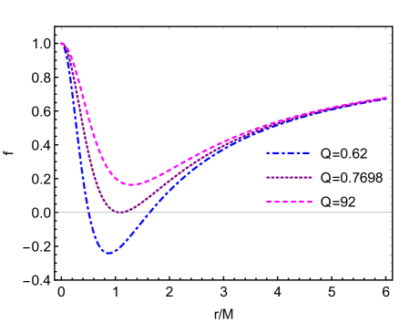
Figure 7: The three conditions of metric function of Bardeen spacetime.

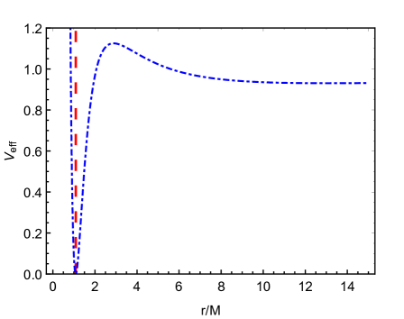
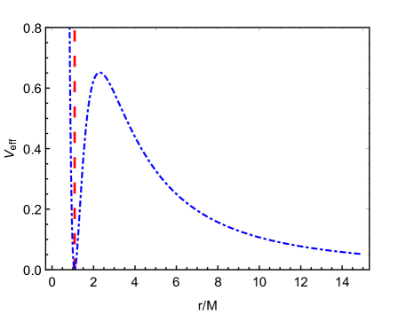
Figure 8: Plot of effective potential in timelike (left) and null geodesics (right) in the extremal $4d$ Bardeen black hole. The dashed red line refers to their respective event horizon.

When extended to $5d$ the metric (43) describes a nonsingular black string. The appearance of $J$ creates a new dynamics different from its $4d$ counterpart, as can be seen in Fig. 9 and 10. As in the RN case, we shall analyze the circular (timelike and null) orbits before obtaining the geodesic’s exact solutions.

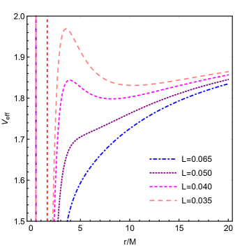
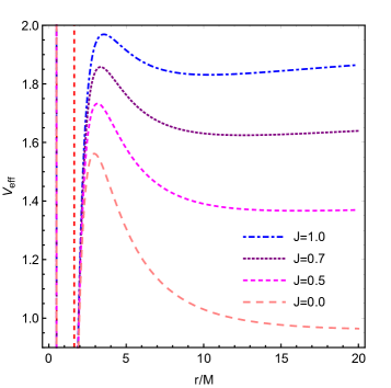
Figure 9: [Left] Plot of effective potential for massive particles in $5d$ two-horizon case with $Q=0.62$ and $J=1$ and various values of $L$ and [Right] similar plot with $L=0.035$ and various values of $J$. The dashed red lines refer to the inner and outer horizons.

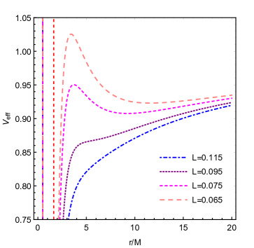
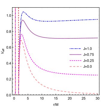
Figure 10: [Left] Plot of effective potential for null particles in $5d$ two-horizon case with $Q=0.62$ and $J=1$ and various values of $L$ and [Right] similar plot with $L=0.063$ and various values of $J$. The dashed red lines refer to the inner and outer horizons.

V.1 Timelike Circular Orbit

Applying the condition (III.1) for the black string yields

$$\left(J+1-\mathbb{E}^{2}\right)Lr_{CO}^{2}\left(r_{CO}^{2}+Q^{2}\right)^{3/2}-2M\left(J+1\right)Lr_{CO}^{4}+\left(r_{CO}^{2}+Q^{2}\right)^{3/2}-2Mr_{CO}^{2} = 0,$$

$$\left(J+1\right)MLr_{CO}^{6}-\left(r_{CO}^{2}+Q^{2}\right)^{5/2}+\left[3+2\left(J+1\right)LQ\right]Mr_{CO}^{4} = 0.$$

One can easily verify that upon $J\rightarrow 0$ they reduce to the MBO conditions for $4d$ Bardeen black hole Gao:2020wjz . Solving them for $L$ and $\mathbb{E}^{2}$ yield

$$L = \frac{\left(Q^{2}+r_{CO}^{2}\right)^{5/2}-3Mr_{CO}^{4}}{(J+1)Mr_{CO}^{4}\left(r_{CO}^{2}-2Q^{2}\right)},$$

$$\mathbb{E}^{2} = \frac{(J+1)\left(Q^{2}\left(3r_{CO}^{4}-4Mr_{CO}^{2}A\right)+4Mr_{CO}^{4}\left(M-A\right)+Q^{6}+3Q^{4}r_{CO}^{2}+r_{CO}^{6}\right)}{-3Mr_{CO}^{4}A+Q^{6}+3Q^{4}r_{CO}^{2}+3Q^{2}r_{CO}^{4}+r_{CO}^{6}},$$

where $A\equiv\sqrt{Q^{2}+r_{CO}^{2}}$.

The ISCO condition gives the additional condition:

$$3\left(Q^{2}+r_{ISCO}^{2}\right)^{7/2}+Mr_{ISCO}^{4}\bigg{[}-2(J+1)LQ^{4}+Q^{2}\left(11(J+1)Lr_{ISCO}^{2}+3\right)$$

$$-2r_{ISCO}^{2}\left((J+1)Lr_{ISCO}^{2}+6\right)\bigg{]}=0.$$

In the extremal case, $Q^{2}=16/27$, the condition becomes

$$2(J+1)LMr_{ISCO}^{8}+2M\left[3\frac{88}{27}(J+1)LM^{2}\right]r_{ISCO}^{6}+{16M^{3}\over 9}\left[\frac{32}{81}(J+1)LM^{2}-5\right]r_{ISCO}^{4}$$

$$-\frac{512M^{5}r_{ISCO}^{2}}{243}+3\left(\frac{16M^{2}}{27}+r_{ISCO}^{2}\right)^{2}\left[2Mr_{ISCO}^{2}-\left(\frac{16M^{2}}{27}+r_{ISCO}^{2}\right)^{3/2}\right]=0,$$

which can be determined numerically.

V.2 Null Circular Orbit

Null geodesic in $4d$ Bardeen spacetime has been discussed widely, for example in Eiroa:2010wm ; He:2021htq . In $5d$ by defining $b^{2}$ and $j$, and by rescaling the proper time the effective potential can be written as

$$V_{eff}=\left(1-\frac{2Mr^{2}}{(r^{2}+Q^{2})^{3/2}}\right)\left(j+{1\over r^{2}}\right).$$ (51)

One can see that the appearance of $j$-term implies the existence of another turning point in $V_{eff}$ outside the horizon, as can be seen in Fig. 10. The CO radii are determined by the roots of the following equation

$$2Mr_{CO}^{4}\left(j\left(r_{CO}^{2}-2Q^{2}\right)+3\right)-2\left(Q^{2}+r_{CO}^{2}\right)^{5/2}=0.$$ (52)

For the extremal case, the condition becomes

$$-81\sqrt{3}Mr_{CO}^{4}\left(JL\left(32M^{2}-27r_{CO}^{2}\right)-81\right)-\left(16M^{2}+27r_{CO}^{2}\right)^{5/2}=0.$$

Both conditions are polynomial equations of degree six, and the roots can best be found numerically.

V.3 Exact Solutions and the Taxonomy of Bound Orbits

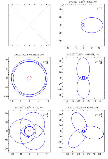
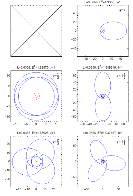
Figure 11: The $z=1,2,3$ orbits in the timelike condition: extremal case with $w=0$ for the first column and $w=1$ for the second column; two-horizon case with $w=0$ for the third column and $w=1$ for the fourth column. Note that the first entries in the first and third column are blank because the $q=0+\frac{0}{1}$ orbits are inaccessible.

Unlike the RN case, we have been unable to cast Eq. (5) into a form that can be solved analytically,

$$\bigg{(}\frac{dr}{d\phi}\bigg{)}^{2}=\frac{2\left(r^{6}L(J+\epsilon)+r^{4}\right)}{\left(Q^{2}+r^{2}\right)^{3/2}}+r^{4}L\left(\mathbb{E}^{2}+J+\epsilon\right)-r^{2}.$$ (54)

To solve it numerically in Mathematica, it is better to rewrite it in terms of the $2^{nd}$-order ODE:

$$\frac{d^{2}r}{d\phi^{2}} = \frac{3Lr^{7}(J+\epsilon)}{\left(Q^{2}+r^{2}\right)^{5/2}}+\frac{3r^{5}\left(2Q^{2}L(J+\epsilon)-1\right)}{\left(Q^{2}+r^{2}\right)^{5/2}}$$ (55)

$$+r^{3}\left(\frac{4}{\left(Q^{2}+r^{2}\right)^{3/2}}-2L\left(-\mathbb{E}^{2}+J+\epsilon\right)\right)-r.$$

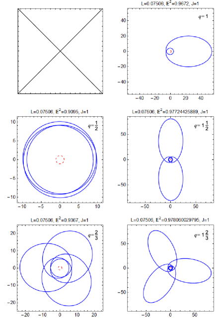
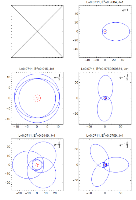
Figure 12: The $z=1,2,3$ orbits in the null condition: extremal case with $w=0$ for the first column and $w=1$ for the second column; two-horizon case with $w=0$ for the third column and $w=1$ for the fourth column. Note that the first entries in the first and third column are blank because the $q=0+\frac{0}{1}$ orbits are inaccessible.

We obtain the numerical solutions of periodic orbits, both for timelike as well as null conditions. They are shown up to $q=1{2\over 3}$ in Figs. 11-12, respectively. For each case we are able to obtain the extremal and two-horizon solutions. What is interesting is that the orbits found in extremal and two-horizon case have almost identical form for each equivalent counterpart.

$q$ SCO 1/2 2/3 1 1 1/2 1 2/3 UCO $\mathbb{E}$ (Extremal) Position 1.815650000 0.00% 1.816250000 0.44% 1.870600000 39.88% 1.929300000 82.48% 1.949485900 97.13% 1.951050000 98.27% 1.953438690 100.00% $\mathbb{E}$ (Two-Horizon) Position 1.827332000 0.00% 1.829750000 1.95% 1.889250000 49.86% 1.935600000 87.18% 1.949349000 98.25% 1.950209151 98.94% 1.951519700 100.00% Deviation - 1.07% 7.06% 3.32% 0.79% 0.48% -

Table 6: Comparison of energy level and the position of particular orbit inside the energy range as percentage for timelike case in extremal and two-horizon nonsingular black string. SCO refers to the bottom level of energy range (no whirl), while UCO refers to the top one (maximum whirl).

To create a more comprehensive view of periodic orbits in the nonsingular string, we provide similar tables as in IV.4. Tables 6 and 7 show various energy levels and each of their corresponding position in extremal and two-horizon cases, respectively. A quick calculation of average of standard deviation of each case would give $0.09\%$ for extremal and $0.07\%$ for two horizon one. This is way smaller than the ones found in RN black string, which means the prediction for the position of each periodic orbit will be more precise in the nonsingular black string.

$q$ SCO 1/2 2/3 1 1 1/2 1 2/3 UCO $\mathbb{E}$ (Extremal) Position 0.908371200 0.00% 0.908659500 0.41% 0.936700000 39.96% 0.967200000 82.98% 0.977244258 97.14% 0.978060029 98.29% 0.979268855 100.00% $\mathbb{E}$ (Two-Horizon) Position 0.913804300 0.00% 0.915000000 1.91% 0.944900000 49.68% 0.968400000 87.23% 0.975259983 98.19% 0.975842810 99.12% 0.976394418 100.00% Deviation - 1.06% 6.88% 3.01% 0.74% 0.58% -

Table 7: Comparison of energy level and the position of particular orbit inside the energy range as percentage for null case in extremal and two-horizon Bardeen black string. SCO refers to the bottom level of energy range (no whirl), while UCO refers to the top one (maximum whirl).

Another point to be noted is that the average of deviation for timelike and null condition is $2.54\%$ and $2.45\%$, respectively. This is a similar manner found in RN black string: the distance between energy levels is more consistent when we compare each specific horizon case, which means this behavior exists generally on charged black holes. By carefully inspecting the numbers from both table, we also find that the orbits in two-horizon condition are more dense toward the local maximum (point of UCO). This behavior is observed in both timelike and null orbits. Nevertheless, one might notice that in the two-horizon nonsingular black string the shift is less drastic compared to similar behavior in two-horizon RN IV.4 where the orbits become highly condensed near the maximum.

As in the timelike RN, the accumulated radial angle can be calculated as follows:

$$\Delta\varphi_{r}=2\int_{r_{p}}^{r_{a}}\frac{\dot{\phi}}{\dot{r}}dr=2\int_{r_{p}}^{r_{a}}\frac{dr}{Lr^{2}\sqrt{\mathbb{E}^{2}-\left(1-\frac{2Mr^{2}}{(r^{2}+Q^{2})^{3/2}}\right)\left(\epsilon+J+\frac{1}{Lr^{2}}\right)}}.$$ (56)

We calculate numerically the accumulated angle and show it in Table 8. We compare the angles we calculate with the corresponding angle from the $4d$ counterpart. As in the RN case, the nonsingular black strings exhibits higher values for the accumulated angle. From the Table 8 the $4d$ angles reach maximum at $q=1{1\over 2}$, then decreases. the $5d$ counterpart, however, keeps increasing as $q$ increasing.

q	$\Delta\varphi_{r-2\ horizon}$	$\Delta\varphi_{r-extremal}$	$\Delta\varphi_{r-4dextremal}$
1/2	50.3815	49.8285	-
2/3	55.5692	54.0185	37.9724
1	66.6127	64.715	44.4775
1 1/2	83.3911	81.0931	50.7586
1 2/3	87.6954	85.7237	48.5055

Table 8: Accumulated angles for the nonsingular black strings. The second and third columns are the angles for 2-horizon and extremal string, respectively. The fourth column is the corresponding angles in the $4d$ extremal Bardeen BH from Gao:2020wjz . The angle for $q=1/2$ in $4d$ extremal Bardeen is empty because the authors do not show solutions for $(2,0,1)$.

VI Conclusion

This works deals with the bound orbits of massive and massless particles around charged RN and nonsingular black strings. These toy models are quite simple, but the geodesics are rich enough to have genuine observables that can be distinguished from their $4d$ counterparts. Following Hackmann Hackmann:2010tqa the RN bound orbits can be expressed analytically in terms of the Weierstrass function, while the nonsingular string must be solved numerically. We present solutions for timelike and null bound orbits in both models, characterized by the rational number $q$. We investigate bond orbit solutions for several $q$ up to $q=1{2\over 3}$. Higher values of $q$ can, in principle, be obtained easily.

What is novel here are twofold. First, the existence of stable bound orbits for photon which does not exist in its 4d counterpart. The addition of (trivial) extra dimension modifies the geodesic equations and thus the shapes of the corresponding $V_{eff}$. As can be seen from Figs. 4 and 10, the non-zero $J$ raises the tail of $V_{eff}$ to create a local maxima outside the corresponding horizons. This is confirmed, for example in the case of RN, by Eq. (28) where the existence of $j\equiv JL$ gives a cubic term in the circular orbit condition. This another extremum turns out to be minimum and lies outside the corresponding horizon(s). Thus this extra bound orbit is stable and observable. For the extremal RN the roots for the cubic equation can be found analytically, as shown in Eq. (29). All $r_{CO}$s are located outside or on the extremal horizon, provided $0<j<1/8M^{2}$.

For the massive case, we show that the circular orbits require higher particle’s energy and angular momentum (remember that the angular momentum $\mathbb{L}\equiv 1/\sqrt{L}$). The ISCO radii are indistinguishable from its $4d$ counterpart. However, as pointed out by authors of Babar:2017gsg , the accumulated angle of the timelike orbit might provide observational signature that can distinguish these black strings from their corresponding black hole counterparts. In Tables 4-5 and 8 we show comparison of radial accumulated angles for black strings and black holes, both for the RN and the nonsingular, respectively. In all cases, the black string accumulated angles are higher compared to the black holes. Thus, measuring such angle for bound orbits of stars around some black hole might give a hint on whether our universe is higher-dimensional or not.

It is probably worthwhile to comment on the size of extra dimension. While the existence of black string solution itself is oblivion to the extra-dimensional size, stability prefers it to be compact, not infinite Gregory:1987nb ; Harmark:2007md . The bounds comes from particle physics as well as cosmology. From particle physics, recent report by CMS collaboration suggests that the size for one “large” extra dimension based on the Randall-Sundrum scenario Randall:1999ee ; Randall:1999vf is of order $\sim 10^{-4}$ fm CMS:2022pjv . A much more optimistic bounds comes from cosmology. Upper bounds value for the emission ring and the angular shadow diameter from the EHT observation on SgrA* indicates that the extra dimension might be as large as $\sim 0.4$ mm Tang:2022hsu .

In this work we only consider static charged black strings in the simplest extension. It would be interesting to extend our investigation to black strings endowed with NLED charged, to regular black strings beyond the Bardeen solutions, or to black strings possessing Lorentz boost as in Gregory:1995qh . We are addressing those issues in the forthcoming works.

Data Availability Statement

Data sharing is not applicable to this article as no data sets were generated or analyzed during the current study.

References

-
(1)
T. Kaluza,
Sitzungsber. Preuss. Akad. Wiss. Berlin (Math. Phys. ) 1921, 966-972 (1921);
O. Klein, Nature 118, 516 (1926) - (2) F. R. Tangherlini, Nuovo Cim. 27, 636-651 (1963)
- (3) R. C. Myers and M. J. Perry, Annals Phys. 172, 304 (1986)
- (4) R. Gregory and R. Laflamme, Phys. Rev. D 37, 305 (1988).
- (5) G. W. Gibbons and K. i. Maeda, Nucl. Phys. B 298 (1988), 741-775 G. T. Horowitz and A. Strominger, Nucl. Phys. B 360 (1991), 197-209 R. Gregory and R. Laflamme,
- (6) R. Gregory, Nucl. Phys. B 467 (1996), 159-182 [arXiv:hep-th/9510202 [hep-th]].
- (7) R. Emparan and H. S. Reall, Phys. Rev. Lett. 88 (2002), 101101 [arXiv:hep-th/0110260 [hep-th]]. R. Emparan and H. S. Reall, Class. Quant. Grav. 23 (2006), R169 [arXiv:hep-th/0608012 [hep-th]]. R. Emparan and H. S. Reall, Living Rev. Rel. 11 (2008), 6 [arXiv:0801.3471 [hep-th]].
- (8) B. P. Abbott et al. [LIGO Scientific and Virgo], Phys. Rev. Lett. 116 (2016) no.6, 061102 [arXiv:1602.03837 [gr-qc]].
- (9) R. Abuter et al. [GRAVITY], Astron. Astrophys. 636 (2020), L5 [arXiv:2004.07187 [astro-ph.GA]].
- (10) K. Akiyama et al. [Event Horizon Telescope], Astrophys. J. Lett. 875 (2019), L1 [arXiv:1906.11238 [astro-ph.GA]].
- (11) K. Akiyama et al. [Event Horizon Telescope], Astrophys. J. Lett. 930 (2022) no.2, L12
- (12) R. Abuter et al. [GRAVITY], Astron. Astrophys. 618, (2018), L10
- (13) Hagihara, Y. 1930, Japanese Journal of Astronomy and Geophysics, 8, 67
- (14) E. Hackmann, PhD dissertation, Bremen University (2010), 256 p. E. Hackmann, B. Hartmann, C. Lammerzahl and P. Sirimachan, Phys. Rev. D 82, 044024 (2010). [arXiv:1006.1761 [gr-qc]].
- (15) S. Grunau and B. Khamesra, Phys. Rev. D 87, no.12, 124019 (2013). [arXiv:1303.6863 [gr-qc]].
- (16) S. Rezvanjou, S. Soroushfar, R. Saffari and M. Masoudi, Class. Quant. Grav. 37 (2020) no.18, 185008 [arXiv:1707.02817 [gr-qc]].
- (17) J. Levin and G. Perez-Giz, Phys. Rev. D 77 (2008), 103005 [arXiv:0802.0459 [gr-qc]].
- (18) J. Levin and B. Grossman, Phys. Rev. D 79 (2009), 043016 [arXiv:0809.3838 [gr-qc]].
- (19) G. Perez-Giz and J. Levin, Phys. Rev. D 79 (2009), 124014 [arXiv:0811.3815 [gr-qc]].
- (20) J. Healy, J. Levin and D. Shoemaker, Phys. Rev. Lett. 103 (2009), 131101 [arXiv:0907.0671 [gr-qc]].
- (21) V. Misra and J. Levin, Phys. Rev. D 82, 083001 (2010) [arXiv:1007.2699 [gr-qc]].
- (22) J. M. Bardeen. in Conference Proceedings of GR5 (Tbilisi, USSR, 1968), p. 174.
- (23) T. Ono, T. Suzuki, N. Fushimi, K. Yamada and H. Asada, EPL 111 (2015) no.3, 30008 [arXiv:1508.00101 [gr-qc]].
- (24) J. Levin, Class. Quant. Grav. 26 (2009), 235010 [arXiv:0907.5195 [gr-qc]].
- (25) G. Z. Babar, A. Z. Babar and Y. K. Lim, Phys. Rev. D 96 (2017) no.8, 084052 doi:10.1103/PhysRevD.96.084052 [arXiv:1710.09581 [gr-qc]].
- (26) A. Cisterna, G. Giribet, J. Oliva and K. Pallikaris, Phys. Rev. D 101 (2020) no.12, 124041 [arXiv:2004.05474 [hep-th]].
- (27) A. Cisterna, C. Henríquez-Báez, N. Mora and L. Sanhueza, Phys. Rev. D 104 (2021) no.6, 064055 [arXiv:2105.04239 [gr-qc]].
- (28) D. Pugliese, H. Quevedo and R. Ruffini, Phys. Rev. D 83 (2011), 024021 [arXiv:1012.5411 [astro-ph.HE]].
- (29) K. Schroven and S. Grunau, Phys. Rev. D 103 (2021) no.2, 024016 [arXiv:2007.08823 [gr-qc]].
- (30) P. Pradhan and P. Majumdar, Phys. Lett. A 375 (2011), 474-479 [arXiv:1001.0359 [gr-qc]].
- (31) F. S. Khoo and Y. C. Ong, Class. Quant. Grav. 33 (2016) no.23, 235002 [erratum: Class. Quant. Grav. 34 (2017) no.21, 219501] [arXiv:1605.05774 [gr-qc]].
- (32) S. Grunau and V. Kagramanova, Phys. Rev. D 83, 044009 (2011). [arXiv:1011.5399 [gr-qc]].
- (33) S. A. Hayward, Phys. Rev. Lett. 96, 031103 (2006) [arXiv:gr-qc/0506126 [gr-qc]].
- (34) A. Bogojevic and D. Stojkovic, Phys. Rev. D 61, 084011 (2000) [arXiv:gr-qc/9804070 [gr-qc]].
- (35) C. Bambi and L. Modesto, Phys. Lett. B 721, 329-334 (2013) [arXiv:1302.6075 [gr-qc]].
- (36) S. G. Ghosh and S. D. Maharaj, Eur. Phys. J. C 75, 7 (2015) [arXiv:1410.4043 [gr-qc]].
- (37) B. Toshmatov, B. Ahmedov, A. Abdujabbarov and Z. Stuchlik, Phys. Rev. D 89, no.10, 104017 (2014) [arXiv:1404.6443 [gr-qc]].
- (38) I. Dymnikova and E. Galaktionov, Class. Quant. Grav. 32, no.16, 165015 (2015) [arXiv:1510.01353 [gr-qc]].
- (39) A. Abdujabbarov, M. Amir, B. Ahmedov and S. G. Ghosh, Phys. Rev. D 93, no.10, 104004 (2016) [arXiv:1604.03809 [gr-qc]].
- (40) E. Ayon-Beato and A. Garcia, Phys. Lett. B 493 (2000), 149-152 [arXiv:gr-qc/0009077 [gr-qc]].
- (41) R. Penrose, Phys. Rev. Lett. 14 (1965), 57-59
- (42) Z. Li and C. Bambi, Phys. Rev. D 87 (2013) no.12, 124022 [arXiv:1304.6592 [gr-qc]].
- (43) B. Gao and X. M. Deng, Annals Phys. 418 (2020), 168194
- (44) E. F. Eiroa and C. M. Sendra, Class. Quant. Grav. 28 (2011), 085008 [arXiv:1011.2455 [gr-qc]].
- (45) K. J. He, S. Guo, S. C. Tan and G. P. Li, Chin. Phys. C 46 (2022) no.8, 085106 [arXiv:2103.13664 [hep-th]].
- (46) T. Harmark, V. Niarchos and N. A. Obers, Class. Quant. Grav. 24 (2007), R1-R90 [arXiv:hep-th/0701022 [hep-th]].
- (47) L. Randall and R. Sundrum, Phys. Rev. Lett. 83 (1999), 3370-3373 [arXiv:hep-ph/9905221 [hep-ph]].
- (48) L. Randall and R. Sundrum, Phys. Rev. Lett. 83 (1999), 4690-4693 [arXiv:hep-th/9906064 [hep-th]].
- (49) [CMS], [arXiv:2210.00043 [hep-ex]].
- (50) Z. Y. Tang, X. M. Kuang, B. Wang and W. L. Qian, [arXiv:2206.08608 [gr-qc]].