Assessing the accuracy of the Australian Senate count

1 Introduction

Australian paper-based elections counted in a polling place are carefully designed to be both privacy-preserving and verifiable. Scrutineers can watch each voter put a ballot paper in each box (one for the Senate and one for the House of Representatives), then watch the manual count of first preferences, or the two-candidate-preferred count, after the polls close. The counting of postal votes can also be scrutinised, although postal voting entails considerable trust in the postal service.

Senate votes are electronically counted after the ballot papers are scanned and the scans transformed into digital preferences in a hybrid human-automated process. The count itself is easy to check, because the Australian Electoral Commission (AEC) publishes detailed digitised preferences, and there are several open-source Senate counting implementations that allow anyone to redo the count.

This paper is therefore not about verifying the count, but about auditing the scanning and digitisation of the Senate ballot papers. Although scrutineers are allowed to observe the automated scanning and partially automated digitisation process, there remains an important evidence gap: scanners are trusted to produce an accurate image of each ballot, software is trusted to retain the images correctly, the digitisation process is trusted to properly digitise, and the digital preferences are assumed to be accurately output, but scrutineers cannot meaningfully observe whether any of this is done correctly. The process can fail in many ways. Images could be inaccurate. Characters could be misinterpreted (by humans or computers). And incorrect or insecure recording and storage of preference data could alter, delete, or add preferences. Thus, undetected software errors or security problems may cause the digitised preferences to differ from the paper ballots. For example, bugs have been discovered in scanners that alter numbers in documents. Even random errors may not be politically neutral [BCS⁺20a].

This risk will be significantly reduced by the recently passed Electoral Legislation Amendment (Assurance of Senate Counting) Bill 2021. The bill mandates an audit of the ballot papers, to compare them with the corresponding digitised preferences and establish an estimate of the overall error rate. It is significant that the law specifies an audit of ballot papers, so that even problems associated with imperfect or insecure scanning can be detected. This is a tremendous opportunity to earn public trust by providing evidence of an accurate process.

Of course, the audit has to be carefully designed to allow for genuine scrutiny. In this guide, we give a short summary of the motivation for auditing paper ballots, explain the necessary supporting steps for a rigorous and transparent audit, and suggest some statistical methods that would be appropriate for the Australian Senate. Our aim is to fill in the AEC’s published methodology sketch with some more of the relevant statistical and computational details.

Update: This version (22 June 2022) now includes analysis of the Senate preference data for the 2022 Australian election. See Section 3.3.3.

1.1 What is auditing?

The aim of an election audit is to ascertain whether the election result was altered by errors, regardless of their cause. The audit should conclude either that there is sufficient evidence that the error rate is low enough that the results deserve to be trusted, or otherwise alert us that errors might be numerous enough to change the results, so the ballots should be examined more carefully. Like the election, the audit is conducted in such a way that election scrutineers can observe and check that it is being conducted correctly.

The AEC already keeps a careful record that connects each ballot paper to its digital preference list. If there were infinite resources, we could examine this correspondence thoroughly by employing a separate team to compare every single ballot paper with its digital preferences, in the presence of scrutineers. However, this would be much too labor intensive to be practical. Instead, a good approximation can be made by an audit that takes a random sample of ballot papers and, for each sampled ballot paper, compares it to its digitised preferences. An error is any discrepancy between the digitised preferences and the marks on the ballot paper, as interpreted by the people conducting the audit.

Of course, not all errors matter. For example, for the Senate, many preferences are not even counted. Also, errors that advantage the apparent winners usually will not be of concern, nor will errors that affect a candidate who is nowhere close to winning, if they are not too numerous. However, in the Senate count it can be very difficult in general to assess whether a group of errors might alter the outcome. Hence we recommend that the audit estimate the average number of errors per ballot and the percentage of ballots that have at least one error, separately in each state or territory. If the error rate is high, suggested ways of dealing with the situation are described below.

An audit should be able to detect errors or malfeasance in any part of the digitisation process. It is not appropriate to reuse any part of the software or hardware used for the initial digitisation. A compromise of, or error in, those systems would cause a corresponding error in the audit.

All parts of the digitisation process should be amenable for auditing, in the sense that every possible failure should be detectable, at least with some probability, by the audit process. For example, the audit should be able to detect if a scanner does not produce accurate images, or if the images are altered after they are produced, or if the preference data are not securely stored. This is why it is important to commit in advance to the system’s output, in the form of digitised preferences, and then to allow scrutineers to observe the retrieval and comparison of the ballot papers. Scrutineers should be encouraged to keep their own records using software of their choice.

Scrutineers need to be able to observe:

1. that the audited ballot papers are chosen randomly, after the digitised preferences are committed to;

2. that the proper ballot papers are retrieved and read;

3. the written marks on the ballot paper;

4. how the written marks compare with the digitised preferences.

This sequence of steps shows scrutineers evidence that the audit is being conducted correctly, and allows them to make their own estimate of the error rate if they wish.

1.2 Ballot paper physical security

This guide describes an auditing process for ballot papers, but of course this would be meaningless without a secure process for accepting, transporting, and keeping track of ballot papers. We understand that the AEC already counts first preferences in the polling place, keeps a record of where each ballot box is sent, and (physically) attaches a unique number to each ballot paper, which is also reflected through the electronic process.

These physical security processes are the crucial assumption on which the audit is based and, although we do not detail them here, the audit relies upon them. For example, when a ballot arrives for processing its physical security needs to be established: scrutineers should be able to observe whichever processes the AEC uses, such as verifying physical seals on the ballot box, reconciling the number of ballots in each batch, checking chain-of-custody documents, logging the examination, etc.

1.3 Generating trustworthy random ballot selections

The sequence of ballots to be audited needs to be chosen transparently and unpredictably. This is necessary to avoid any (real or perceived) possibility that the sampling might not be truly random—unpredictability is necessary to prevent malicious software from hiding misrecordings in ballots that will not be audited. Fortunately there are numerous methods for generating pseudorandom sequences of numbers in a transparent, yet unpredictable way.

The key idea is to use a random seed to start a transparent process. The AEC should commit in advance to the algorithm that will transform the seed into a sequence of ballot selections, and to the method by which that seed will be chosen. For example, the seed could be derived from a series of dice rolls, or a physical machine such as the one used to draw candidate order on ballot papers. The actual draw should not happen until after the batch has been processed (see below). It should be generated in public view so that scrutineers can see that it cannot be determined in advance.

Since each state or territory audit is conducted separately, a random seed should be generated separately in each central counting centre, under observation by the scrutineers who are present.

The method for deriving a sequence of ballot selections from the seed should also be published in advance, in the form of openly available computer code for a specific algorithm that scrutineers can re-run for themselves. This allows scrutineers to verify that the sequence of ballot selections has been made properly based on the seed.

2 The steps of an audit

The Senate election consists of eight simultaneous but separate contests, one for each state and territory. These will each have different candidates and ballots, and potentially different error rates because they are counted using separate equipment. On that basis, we recommend treating each contest separately.

The precision of the error estimate is related to the sample size in each state or territory. Also, the sources of error may be specific to a particular counting centre. Therefore, we recommend initially sampling approximately the same number of ballot papers from each state and territory, even though some will have many more ballots than others. This produces an estimate of the error rate in each state or territory, which may be sufficient to conclude the audit in many cases.

However, in the event of either high error rates or very close outcomes, it may be necessary to take more samples later. This requires completing the digitisation of all the ballots, in order to estimate the closeness of the contest, and then deciding whether a larger sample is required for the necessary level of confidence.

This section contains an overview of the steps of the audit of the ballot digitisation process, for each state or territory. Figure 1 shows a diagram of the process. Section 3 contains more details about each step.

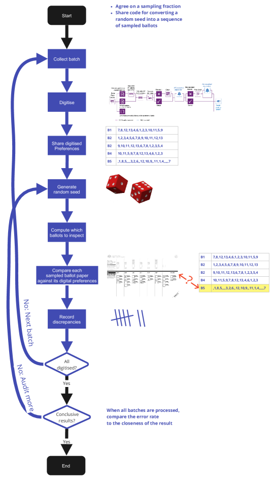
Figure 1: Flowchart of Senate auditing process. Image of Senate scanning process from Australian National Audit Office. Image of sample ballot paper from AEC. https://www.aec.gov.au/voting/how_to_vote/files/senate-btl-sample.png. Creative Commons License.

2.1 In advance

In advance, publish the audit methodology, including:

• the process for generating a random seed,

• the algorithm for deriving a sequence of ballot choices from that seed, including any software that will be used (‘sampling software’),

• the process for recording errors, including any software that will be used (‘auditing software’),

• the algorithm for finding confidence bounds on the error rates from the sample,

• the steps to be taken if the audit shows a high rate of error and more samples need to be taken.

2.2 Preparation on the day

• Calculate a sampling fraction based on the threshold in the Electoral Act 1918, the expected error rates, desired confidence level, etc., and configure sampling software accordingly.

• Report (commit to) the final turnout by polling place before any ballots from a given polling place are processed.

Detailed suggestions are in Section 3.2.

2.3 Processing and auditing each batch of ballots

• Open the batch, scan it, run it through the digitisation process, generate digitised preferences.

• Share the digitised preferences with scrutineers, with an index number matching that of the ballot paper.

• Generate a random seed in a public ceremony.

• Use the sampling software, with the random seed, to determine which ballots to sample from the current batch.

• Retrieve these ballots from the batch.

• Inspect these ballots and enter the human reading into the auditing software, which records any discrepancies.

• Ensure that scrutineers can see what ballots have been selected by the sampling software, can verify that those ballots are the ballots examined, and can compare each to its digitised preferences.

Detailed suggestions are in Section 3.2.

2.4 Analysing the results and concluding the audit

• After the final batch, verify that all validly cast ballots have been accounted for and scanned (in a way that scrutineers can check).

• Use the auditing software to compute and report a confidence interval for the error rate.

• Make a best-effort computation of the election margin.

• If necessary, sample more ballots for any contests in which the audit results are inconclusive.

• Determine a conclusion and recommendation given the outcomes of the previous steps.

Detailed suggestions are in Section 3.3.

Depending on the exact details of AEC paper-ballot processes, there should also be concluding double-checks to make ensure that every ballot has been through this process and could have been selected to be in the sample by the sampling software. There should be a reconciliation of numbers, e.g. that the number of ballot papers from a given polling place matches the number of eligible voters marked off on the rolls at that place.

3 Details of each step

3.1 Before the election: publishing the methodology and process

Section 273(AC)(6) states:

Before the polling day for the election, the Electoral Commissioner must publish on the Electoral Commission’s website:

1. the methodology to be used for the ballot paper sampling process; and

2. the process to be used for reconciling preferences.

The following sections provide specific suggestions for each of these requirements.

3.2 Conducting the audit

273(AC)(2) of the Electoral Act 1918 states:

The Electoral Commissioner must arrange for statistically significant samples of ballot papers to be checked throughout the scrutiny of votes for the election to assure that the electronic data used in counting the votes reflects the data recorded on the ballot papers.

Paragraph (3) requires at least 5,000 ballots to be sampled overall, or 1,000 if only one state’s Senate election is running.

It is not specified what “statistically significant” means, nor does it explicitly say that the sample must be random, though we take this to be implicit.

This sampling problem is somewhat different from US-style post-election audits because the language “throughout the scrutiny” suggests that auditing should be conducted progressively while the ballot digitisation is performed. We assume that ballots are audited in batches, with the audit commencing after the batch has been digitised. However, it is also important to be able to revisit older batches and examine more ballot papers if concerns arise.

3.2.1 Generating the sequence of sampled ballots in a transparent way

There are many different algorithmic choices for transparent generation of a random sequence of ballots. We detail one particular option here, because it is very simple and all the software for implementing it is already openly available.

Bernoulli sampling using geometric skipping [OBH⁺20], implements the following idea: from a population of ballots (each with an index number) generate a pseudorandom sequence of ballot numbers to be audited, in such a way that each ballot is equally likely to be chosen, independently of whether other ballots are chosen. Geometric skipping is conveniently designed to skip forward through a sequence of ballots.

The geometric skipping algorithm is parameterised by one value: the probability that each single ballot will be included ($p$). The implementation code also accepts a seed value for the pseudorandom number algorithm. For Senate auditing, the seed would be generated from some public process such as dice rolling (see Section 1.3), and the selection probability $p$ would need to be chosen so that the total sample size was compliant with legislation—this is discussed in the next section.

3.2.2 Achieving the required sample size

The Electoral Act 1918 specifies an overall sample size of at least 5000 ballots, or at least 1000 ballots if only one jurisdiction is running an election at a time. To start with, we show how to set up the sampling to achieve this minimum requirement. In Section 3.3 we offer some suggestions for interpreting the ‘statistically significant’ requirement and explain when a larger sample might be required—this would typically happen for very close contests or large error rates. Our suggestion is to make a first pass throughout the digitisation process, sampling ballots at random from each batch as they are digitised. Ideally, this should be sufficient to have confidence in the results in many cases. However, we may discover at the end of the process that the results are inconclusive, and that more auditing is required. In that case, a second pass is needed, retrieving ballots from storage.

We show two sets of worked examples below. The first is where we aim for a sample of at least 1000 for a single jurisdiction. The second is where we aim for a sample of at least 5000 across all jurisdictions. For the latter, we have split the sampling goal equally across the six states and two territories, by setting a target of at least 625 ballots from each one.

To calculate the required selection probability $p$ for a given a jurisdiction, we need to know the total number of ballots cast in that jurisdiction ($n$) and the target sample size ($t$). The actual sample size ($S$) will follow a binomial distribution ($S\sim\operatorname{Bi}(n,p))$. To ensure that it has at least 99.9% probability of exceeding the target sample size, we can solve the following inequality in terms of $p$:

$$\Pr(S\geqslant t)\geqslant 0.999.$$

This can be done using standard statistical software. Table 1 shows some examples, being minimum values of $p$ that satisfy the inequality.

If the actual sample size ends up being smaller than the target sample size (which can occur but is very unlikely), the sample should be supplemented by sampling sufficiently more ballots at random from all of the cast ballots.

There are other reasonable strategies here, for example aiming for a sample of 400 in each jurisdiction and then allowing the remaining 1800 to be sampled from whichever contests are closest or most error prone. These tradeoffs depend on the error rates, how close each contest is, and how much more effort it is to retrieve a ballot that has been put into storage than one that has just been digitised. The closeness of the result can be known only after the particular contest is digitised—some past Senate elections have been close enough for fewer than 100 votes to alter the outcome, though tens of thousands is more typical.

There is limited information about the error rate of the existing process, though of course more information will be available after this year’s audit. In prior work, we used a variety of techniques to attempt an estimate, arriving at a value somewhere between 0.04% and 0.89% for the per-digit error rate [BCS⁺20b]. The per-ballot error rate would obviously be some multiple of that, because ballots can have hundreds of digits, though typically have fewer than 10.

Table 1: Example minimum values for the selection probability, $p$. The calculations assume all enrolled voters cast a vote. Enrolment numbers are from the AEC, https://www.aec.gov.au/Enrolling_to_vote/Enrolment_stats/national/2021.htm.

		Selection probability ($p$)
State/Territory	Enrolled voters ($n$)	Target: $t=1000$	Target: $t=625$
NSW	5,427,292	0.000202852	0.000129934
VIC	4,305,961	0.000255677	0.000163770
QLD	3,450,635	0.000319053	0.000204365
WA	1,752,273	0.000628288	0.000402441
SA	1,244,611	0.000884557	0.000566591
TAS	397,279	0.002771133	0.001775011
ACT	309,521	0.003556806	0.002278264
NT	145,335	0.007574710	0.004851881

So another reasonable approach is to make a guess at the error rate and the likely closeness of the result, and to compute a sample target that would give us sufficient confidence in the result, if those guesses turned out to be correct. For example, if we assume an error rate of 0.5% and that approximately 1% of votes would need to change in order to change the election result, we could use the techniques described in Section 3.3.1 to choose a sample size so that, if those assumptions were correct, the audit could conclude with confidence that the error rate was low enough, without needing a second pass. This may require a larger first-pass sample, but might be worth the effort to avoid additional passes, which involve time-consuming retrieval from storage. Of course, if the assumptions are shown to be wrong, a second pass may be necessary anyway.

In summary, depending on the relative difficulty of auditing a ballot that has just been digitised vs auditing that same ballot after it has been stored, there are several options:

• target exactly the sample size needed to meet the legislative requirement,

• target a slightly larger sample size, hoping to reduce the number of states or territories that require additional passes,

• target a smaller sample size, expecting to use all of the extra on the one or two states or territories that require additional passes,

• use an estimate of the error rate to choose a sample size that is likely to be large enough to avoid the need for additional passes.

The following discussion is independent of which of these options is chosen.

3.3 Dealing with discrepancies

Software-based processes are human processes, and humans are imperfect and make mistakes. It is possible that the audit will uncover some discrepancies that are enough to alter the outcome, for example because of a systematic error in the processing or a human error in the data uploading. In these cases, it is important to be honest and transparent, and to examine what went wrong while allowing scrutineers to observe the reconciliation process. The legislation does not specify what to do in the event of larger-than-expected error rates, but one obvious option is to audit more so as to get a better estimate. If the error rate seems to be genuinely high, manual examination of all the paper ballots may be required.

The legislation also does not specify what level of error is small enough to be acceptable. In general, tighter contests will be less tolerant of errors, while larger errors may make no difference if the margin is sufficiently large.

The rest of this section explains how to compare the estimated error rate with calculations of how many vote-changes can alter the election outcome.

3.3.1 Estimating the overall error rate

Once the sample of ballots is collected, they are compared to the digitised preferences and the number of errors are recorded. This allows us to estimate the overall error rate. For example, if we observe 30 errors out of 5000 ballots, an estimate of the error rate is $30/5000=0.006=0.6\%$.

In general, this will be close but not equal to the true error rate. To represent the uncertainty of the estimate we can calculate a confidence interval. This will give a range of values (for the true error rate) that are most plausible given the data. For the above example, a 95% confidence interval is (0.0041, 0.0086). In other words, it is implausible that the true error rate is outside the range 0.41% to 0.86%.

The legislation refers to a “statistically significant sample,” without defining what this means. In the current context, a typical interpretation of “statistically significant” would be that the confidence interval excludes some comparison value of interest; we adopt this interpretation in the following sections, where we compare the interval to an estimate of how close the election was (a ‘margin’). Therefore, we interpret “statistically significant sample” to refer to a sample that allows us to estimate the error precisely enough—by producing a narrow enough confidence interval—that it excludes the (margin) value we are comparing it to. The main factor that will determine this is the number of sampled ballots: sampling more ballots leads to narrower confidence intervals. If the initial sample does not give a statistically significant result, we advocate sampling more ballots until statistical significance is achieved (see Section 3.4), as required by the legislation or, if that is not possible, manually re-examining all the ballots to ensure an accurate result.

The ‘95%’ mentioned above is known as the confidence level of the confidence interval. It tell us how reliable the interval is—the higher the confidence level, the more often the confidence interval will include the true value. We can set the confidence level to any value between zero and 100%, but there is a tradeoff: all else equal, to increase the level requires making the confidence interval wider, which would then require more samples to reach statistical significance. A conventional choice through much of scientific research is 95%, and in some contexts it is much higher, but rarely lower.

There are many methods for calculating confidence intervals. They differ in the assumptions they make about how the data are sampled. One should use a method that is consistent with the sampling design and what is known about the population being sampled. The above example used the Clopper–Pearson method, which is widely used and implemented in standard software. The method assumes that the population is binary (each ballot either does or does not have an error), and that the sample size is fixed in advance and drawn ‘with replacement’, which is appropriate for many studies. In the current context, ballots will actually be sampled ‘without replacement’ and the size is not fixed in advance; methods exist that are appropriate for such samples, see [OBH⁺20]. Another difference is that we may need to do more than one round of sampling to obtain a statistically significant estimate. If so, the calculation of the confidence intervals needs to be adapted to take this into account. This requires more advanced methods.

3.3.2 What size error is small enough?

In first-past-the-post elections, where the winner is simply the person who receives the most votes, the error rate can simply be compared to the margin of victory (or just margin), that is the number of ballots that would need to change to change the result. In first-past-the-post elections the margin of victory is half the difference between the tally of the winner and the second highest tally. For example, if 45% of voters reportedly voted for Alice and 35% reportedly voted for Bob, the audit needs to provide confidence that errors affected less than 5% of the ballots. For these simple electoral systems, even more careful accounting is possible—errors that advantage Bob can be disregarded, for example, because they would not change the election outcome. There is an extensive literature on precise, efficient, accounting for different kinds of errors [LS12, Sta20].

Unfortunately, none of these techniques transfers easily to Senate auditing, because it is infeasible to compute election margins, and just as difficult to tell which kinds of errors could make a difference to the outcome. Even if a certain preference was not read during the official count, an alteration in some other ballot may change the elimination order and cause that preference to matter.

However, the error estimation is still valuable. It can provide a good degree of confidence under reasonable assumptions in many scenarios, or, conversely, it can give a meaningful indication that more examination is needed, if the error rate is high.

Although computing exact margins for the Senate count is infeasible in general, there are some straightforward ways to find small changes that are sufficient to change the outcome. For example, in many cases the last seats are allocated when a candidate ($c$) is eliminated, leaving exactly as many continuing candidates as unfilled seats. In this case, it is easy to compute the difference between $c$ and the next-lowest candidate $d$ (who wins a seat). Shifting sufficient votes from $d$ to $c$ obviously changes the outcome—$c$ wins a seat instead of $d$. The required number of votes is called the last-round margin. At any time, the outcome can also be changed by raising up any non-winning candidate until they have a quota.

However, there may be smaller alterations earlier in the elimination sequence that are also sufficient to change the outcome. These are much harder to detect in general, but there are several published heuristic algorithms for finding answers [BCST20, TC]. These programs search for small changes in votes that change the election outcome. If a program finds an example, that change to the votes definitely can change the outcome—but there may be a way to change the outcome by changing fewer votes that the algorithm did not detect. Open-source software for these algorithms are available and could be run routinely on all digitised Senate preferences.

Any of these methods gives a feasible, but not necessarily minimal, way of changing the outcome. We call this number of vote-changes the apparent margin. Evidence that there were fewer errors than the apparent margin is evidence against that particular change in the outcome.

3.3.3 Update (22 June 2022): results for the 2022 Australian Senate election

We have applied some heuristic search algorithms to the openly available vote data supplied by the AEC. Because first preferences are manually counted in the polling place in the presence of scrutineers, the opportunity for them to be altered undetectably by software problems is fairly limited. We therefore give two versions of the smallest-change values: one that allows for first preferences to be altered, and one that is limited to changes in later preferences only. Full results are in Table 2. Instructions for replicating the results are in the source code repository.

State or	Formal	Allow 1st-prefs		No 1st-prefs		Effect
Territory	votes	Change	(%)	Change	(%)
ACT	285217	14137	4.96%	$\times$	$\times$	+Seselja(LP); -Pocock(Ind)
NSW	4800722	57340	1.19%	57340	1.19%	+McCulloch(ON); -Molan(LP)
NT	103617	11412	11.01%	$\times$	$\times$	+Anlezark(Grn); -McCarthy(ALP)
QLD	3013868	54810	1.82%	59428	1.97%	+Stoker(LP);
						-Chisolm (ALP) (1st pref changes)
						-Hanson(ON) (no 1st prefs)
SA	1128524	9306	0.82%	12558	1.11%	+Gill(ALP); -Liddle(LP)
TAS	361048	11697	3.24%	$\times$	$\times$	+Mav(ON); -Tyrrell(JL)
VIC	3821539	9341	0.24%	9341	0.24%	+Pickering(ON); -Babet(UAP)
WA	1526123	11745	0.77%	$\times$	$\times$	+Filing (ON); -Payman (ALP)

Table 2: Vote changes that can change Senate outcomes for 2022 Australian Senate results. Two kinds of changes are shown. ‘Allow 1st-prefs’ lets first-preferences be different. In ‘No 1st-prefs’, first-preferences are assumed to be perfectly recorded. In some cases, this results in a slightly larger number of vote changes, in others it makes no difference, and in some cases it precludes any solution—this is indicated with a ’$\times$’.

Victoria seems to be the closest, with 9341 vote changes, or $0.24\%$, sufficient to change the outcome. Western Australia (0.77%) and South Australia (0.82%) are next. The other states do not seem close—the smallest changes we could find all required more than a $1\%$ vote change. It would therefore make sense to concentrate auditing effort on Victoria, WA and SA. If the error rate is indeed less than $0.5\%$, then we can be fairly confident that the WA and SA results are correct, but it may take a fairly large sample to have confidence that the error rate is sufficiently small. In the case of Victoria, based on previous AEC statements, it is possible that the overall error rate may be larger than the number of changes sufficient to change the outcome. This does not imply that the results are wrong, but it does mean that more extensive re-examination of the ballot papers may be required in order to be confident of the result.

3.4 Concluding the audit

After all the votes have been processed and each batch has been audited, we have both a complete list of digitised preferences and an overall estimate (and confidence interval) of the error rate in each state or territory. In addition, for each state and territory we have an apparent margin: an estimate of the number of ballots that would have to have digitisation errors for the reported electoral outcome to be incorrect.

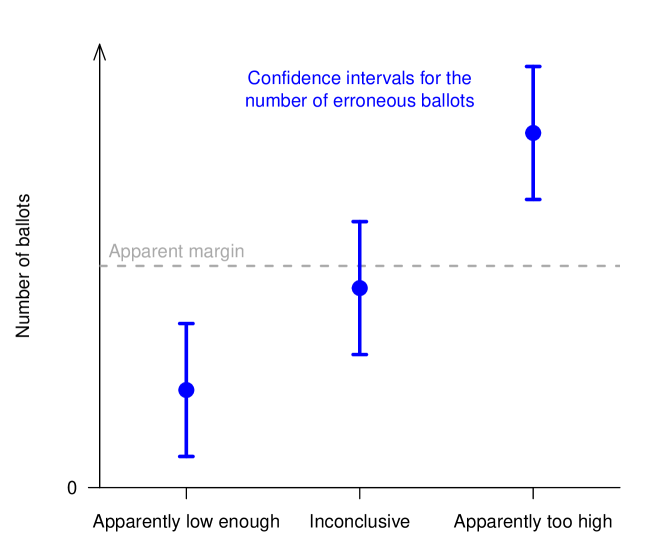
Figure 2: Possible outcome scenarios.

We can multiply the confidence intervals by the number of cast ballots, so they become confidence intervals for the number of ballots with digitisation errors. This allows us to compare them directly with the apparent margins. In each jurisdiction we have one of the following possible scenarios, as illustrated in Figure 2:

• Apparently low enough error rate. The upper endpoint of the confidence interval is below the apparent margin. In this case, it is appropriate to conclude the audit and report that the errors are unlikely to have altered the outcome of the election. (However, the apparent margin may be an overestimate; this should be noted as a caveat in the report.)

• Apparently too high error rate. The lower endpoint of the confidence interval is larger than the apparent margin. This is the difficult case, which may indicate irrelevant errors or a genuine problem: it requires further investigation.

  • Assess the nature of the errors.

  • Investigate potential sources of error. For example, this might lead to an observation that one scanner is of very poor quality, or one computer involved in the digitisation process has been compromised.

  There is no general procedure for dealing with this situation. It requires careful assessment of the nature and causes of the errors and, potentially, re-examination of all the paper ballots.

• Inconclusive error rate. The confidence interval includes the apparent margin. In this case, we have insufficient evidence to say whether the error rate is greater or smaller than the margin; in statistical jargon, the difference between them is said to be ‘not statistically significant’.

  In this case, more auditing should be done to get a more precise estimate of the error rate, to determine with more certainty whether or not it exceeds the margin. This second phase should ensure that all ballots cast in the contest could be sampled with equal probability.

In addition to meeting the legislative requirements, these investigations and outcomes could also be used to defend an election outcome against an accusation that the result is not accurate. A carefully conducted, rigorous demonstration of a low error rate should be convincing evidence that the outcome is correct. A candidate who disputed the results could be invited to produce a specific set of ballot alterations that could allow them to be elected, and if they were unable to produce any within the measured error rate this would be strong evidence against that particular set of errors.

4 Conclusion

Overall, a transparent audit should improve both the real and perceived accuracy and integrity of Australian Senate elections. If done properly, it has the potential either to detect and correct errors, or to demonstrate transparently that the error rate is low enough to support an accurate election result.

References

- [BCS+20a] Michelle Blom, Andrew Conway, Peter J. Stuckey, Vanessa J. Teague, and Damjan Vukcevic. Random errors are not necessarily politically neutral. In Electronic Voting. E-Vote-ID 2020, volume 12455 of Lecture Notes in Computer Science, pages 19–35, Cham, September 2020. Springer. Preprint: arXiv:2007.00854.
- [BCS+20b] Michelle Blom, Andrew Conway, Peter J Stuckey, Vanessa J Teague, and Damjan Vukcevic. Random errors are not necessarily politically neutral. In International Joint Conference on Electronic Voting, pages 19–35. Springer, 2020. https://arxiv.org/abs/2007.00854.
- [BCST20] Michelle Blom, Andrew Conway, Peter J Stuckey, and Vanessa J Teague. Did that lost ballot box cost me a seat? Computing manipulations of STV elections. In Proceedings of the AAAI Conference on Artificial Intelligence, volume 34, pages 13235–13240, 2020. https://web.archive.org/web/20201103172932id_/https://aaai.org/ojs/index.php/AAAI/article/download/7029/6883.
- [HRMS21] Steven R. Howard, Aaditya Ramdas, Jon McAuliffe, and Jasjeet Sekhon. Time-uniform, nonparametric, nonasymptotic confidence sequences. The Annals of Statistics, 49(2):1055–1080, 2021.
- [LS12] Mark Lindeman and Philip B Stark. A gentle introduction to risk-limiting audits. IEEE Security & Privacy, 10(5):42–49, 2012. https://www.stat.berkeley.edu/~stark/Preprints/gentle12.pdf.
- [OBH+20] Kellie Ottoboni, Matthew Bernhard, J. Alex Halderman, Ronald L. Rivest, and Philip B. Stark. Bernoulli ballot polling: A manifest improvement for risk-limiting audits. In Financial Cryptography and Data Security, pages 226–241, Cham, 2020. Springer International Publishing. Preprint: arXiv:1812.06361.
- [Sta20] Philip B Stark. Sets of half-average nulls generate risk-limiting audits: SHANGRLA. In International Conference on Financial Cryptography and Data Security, pages 319–336. Springer, 2020. https://arxiv.org/abs/1911.10035.
- [TC] Vanessa Teague and Andrew Conway. iVote issues: Assessment of potential impacts on the 2021 NSW local government elections. https://github.com/AndrewConway/ConcreteSTV/blob/main/reports/NSWLGE2021Report.pdf.
- [WSSR21] I. Waudby-Smith, P.B. Stark, and A. Ramdas. RiLACS: Risk limiting audits via confidence sequences. In Electronic Voting. E-Vote-ID 2021, volume 12900 of Lecture Notes in Computer Science, pages 124–139, Cham, 2021. Springer Nature. Preprint: arXiv:2107.11323.