Construction of the spectral function from noncommuting spectral moment matrices

Abstract

The LDA+$U$ method is widely used to study the properties of realistic solids with strong electron correlations. One of its main shortcomings is that it does not provide direct access to the temperature dependence of material properties such as the magnetization, the magnetic anisotropy energy, the Dzyaloshinskii-Moriya interaction, the anomalous Hall conductivity, and the spin-orbit torque. While the method of spectral moments allows us in principle to compute these quantities directly at finite temperatures, the standard two-pole approximation can be applied only to Hamiltonians that are effectively of single-band type. We do a first step to explore if the method of spectral moments may replace the LDA+$U$ method in first-principles calculations of correlated solids with many bands in cases where the direct assessment of the temperature dependence of equilibrium and response functions is desired: The spectral moments of many-band Hamiltonians of correlated electrons do not commute and therefore they do not possess a system of common eigenvectors. We show that nevertheless the spectral function may be constructed from the spectral moments by solving a system of coupled non-linear equations. Additionally, we show how to compute the anomalous Hall conductivity of correlated electrons from this spectral function. We demonstrate the method for the Hubbard-Rashba model, where the standard two-pole approximation cannot be applied, because spin-orbit interaction (SOI) couples the spin-up and the spin-down bands. In the quest for new quantum states that arise from the combination of SOI and correlation effects, the Hartree-Fock approximation is frequently used to obtain a first approximation for the phase diagram. We propose that using the many-band generalization of the selfconsistent moment method instead of Hartree-Fock in such exploratory model calculations may improve the accuracy significantly, while keeping the computational burden low.

I Introduction

The LDA+$U$ approach is a very popular method to compute the electronic structure of realistic solids with strong electron correlations [1, 2, 3, 4]. While it is less accurate than dynamical mean field theory (DMFT) [5] it is computationally faster.

Recently, the demand to compute spintronic material properties such as the Dzyaloshinskii-Moriya interaction [6], the spin-orbit torque [7, 8, 9, 10] and the Hall coefficient [11, 12, 13, 14] at finite temperatures has increased. While LDA+DMFT provides direct access to the temperature dependence of equilibrium and response property tensors, the LDA+$U$ scheme is limited to zero temperature unless it is extended by subsequent calculations of the effects of finite temperature e.g. by Monte-Carlo simulations, by classical atomistic spin models, or by Green’s function theory [15, 16, 17]. This poses the question of whether extending LDA+$U$ by additional higher-order correlation functions beyond the mean-field level will allow us to compute these material properties directly at finite temperature with a computational cost comparable to LDA+$U$ calculations, i.e., a computational cost much smaller than the one of LDA+DMFT. This question is particularly important in view of response tensors such as the anomalous Hall effect (AHE) [18, 19, 20] or the spin-orbit torque [21], which often require a much finer $k$-point sampling to achieve convergence than the calculation of total energies and magnetic moments does, e.g. due to the spiky Berry curvature of the AHE.

The self-consistent spectral moment method explored in the eighties on the basis of a single band Hubbard model is an alternative approach able to predict realistic results for the Curie temperatures in Fe and Ni [22, 23, 24] and it is computationally much less demanding than LDA+DMFT. Similarly to LDA+$U$ and LDA+DMFT, it improves LDA by adding a Hubbard-type interaction to it. While the Kubo-Bastin equation for the electrical conductivity [25, 26] does not hold for correlated electrons, the method of spectral moments can also be used to compute the response functions avoiding the independent particle approximation of the Kubo-Bastin equation [27]. In this paper we embark on extending the self-consistent spectral moment approach to a new practical computational method that can be combined with density functional theory to study the finite temperature properties of realistic magnetic materials and spintronic modules. For this we need to go beyond the single band approximation of the original method. The success of our new approach is explicitly shown for the relativistic Rashba Hubbard model. Avoiding the solution of the quantum impurity problem inherent to the LDA-DMFT method, our approach to the finite temperature problem is expected to be computationally much faster.

We define the $n$-th spectral moment matrix at $k$-point ${\bm{k}}$ by [22, 23, 28]

$${\bm{M}}^{(n)}_{{\bm{k}}}=\frac{1}{\hbar}\int_{-\infty}^{\infty}{\bm{S}}_{{\bm{k}}}(E)E^{n}dE,$$ (1)

where ${\bm{S}}_{{\bm{k}}}(E)$ is the spectral density matrix at energy $E$. Since the spectral moments may alternatively be expressed in terms of thermal averages of anticommutators such as [22, 23, 28]

$$\tilde{M}^{(1)}_{{\bm{k}}\alpha\beta}=\frac{1}{N}\sum_{ij}e^{i{\bm{k}}\cdot({\bm{R}}_{i}-{\bm{R}}_{j})}\langle[[c_{i\alpha},\mathcal{H}]_{-},c^{\dagger}_{j\beta}]_{+}\rangle,$$ (2)

where $c^{\dagger}_{j\beta}$ creates an electron in state $\beta$ at lattice site $j$ (position ${\bm{R}}_{j}$), $c_{i\alpha}$ annihilates an electron in state $\alpha$ at lattice site $i$ (position ${\bm{R}}_{i}$), $\mathcal{H}=H-\mu\hat{N}$, $H$ is the Hamiltonian of the system, $\hat{N}$ is the number operator, $\mu$ is the chemical potential, $[\dots]_{-}$ denotes the commutator, and $[\dots]_{+}$ is the anticommutator, a closed system of equations for ${\bm{S}}_{{\bm{k}}}(E)$ may be obtained by requiring that ${\bm{M}}^{(n)}_{{\bm{k}}}=\tilde{{\bm{M}}}^{(n)}_{{\bm{k}}}$. Usually, the first four moments are considered, i.e., n=0, 1, 2, 3. In Eq. (2) we give only the anticommutator for the first moment. The $n$-th moment contains $n$ commutators, which are generated by applying the equation of motion $n$ times. Explicit expressions are given in App. A.

In the single-band Hubbard model the electron can only be in the state of spin up ($\uparrow$) or spin down ($\downarrow$), i.e., $\alpha=\uparrow,\downarrow$, and one may choose the spectral function and the spectral moments to be diagonal in the spin indices, i.e., $M^{(n)}_{{\bm{k}}\alpha\beta}=M^{(n)}_{{\bm{k}}\alpha}\delta_{\alpha\beta}$ and $S_{{\bm{k}}\alpha\beta}=S_{{\bm{k}}\alpha}\delta_{\alpha\beta}$. Considering the first 4 moments – n=0, 1, 2, 3 – one obtains 4 equations for $\alpha=\uparrow$ and 4 equations for $\alpha=\downarrow$. These 4 equations may be used to determine the 4 unknown coefficients $a_{{\bm{k}}\alpha 1}$, $a_{{\bm{k}}\alpha 2}$, $E_{{\bm{k}}\alpha 1}$, and $E_{{\bm{k}}\alpha 2}$ in the two-pole approximation [28]

$$\frac{S_{{\bm{k}}\alpha}(E-\mu)}{\hbar}=a_{{\bm{k}}\alpha 1}\delta(E-E_{{\bm{k}}\alpha 1})+a_{{\bm{k}}\alpha 2}\delta(E-E_{{\bm{k}}\alpha 2})$$ (3)

of the spectral density. Here, $E_{{\bm{k}}\alpha 1}$ and $a_{{\bm{k}}\alpha 1}$ are the band energy and the spectral weight of the lower Hubbard band, while $E_{{\bm{k}}\alpha 2}$ and $a_{{\bm{k}}\alpha 2}$ are those of the upper Hubbard band. The alternative expression of the third moment $M^{(3)}_{{\bm{k}}\uparrow}$ in terms of the thermal average of an anticommutator contains higher-order correlations such as $\langle c^{\dagger}_{i\uparrow}c^{\dagger}_{i\downarrow}c_{j\downarrow}c_{j\uparrow}\rangle$, which lead to a much more realistic description of the effect of finite temperature than the mean field level can provide.

In order to replace LDA+$U$ by the method of spectral moments one might consider to map the electronic structure of a standard LDA calculation first onto a set of maximally localized Wannier functions (MLWFs) [29]. $c_{i\alpha}$ may then be considered to be the annihilation operator of an electron in the MLWF state $|{\bm{R}}_{i}\alpha\rangle$. Note that MLWFs are routinely used for the Wannier interpolation of response functions such as the AHE [20] and the spin-orbit torque [21]. When one wishes to compute such response functions, the mapping of the electronic structure onto MLWFs is therefore often not an additional complication, because this step will have to be done in any case. Some implementations of LDA+$U$ already use Wannier functions as basis set [30].

The question now arises of how to modify Eq. (3) when we have $N_{\rm W}$ states, i.e., $\alpha=1,\dots,N_{\rm W}$ instead of only the two states $\alpha=\uparrow,\downarrow$ in the single-band Hubbard model. An obvious generalization of Eq. (3) is given by

$$\frac{S_{{\bm{k}}\alpha\beta}(E-\mu)}{\hbar}=\sum_{p=1}^{2}\sum_{\gamma=1}^{N_{\rm W}}a_{{\bm{k}}\gamma p}\mathcal{V}_{{\bm{k}}\alpha\gamma p}\mathcal{V}^{*}_{{\bm{k}}\beta\gamma p}\delta(E-E_{{\bm{k}}\gamma p}),$$ (4)

where $p=1$ denotes the lower Hubbard band, while $p=2$ denotes the upper one, and $\mathcal{V}_{{\bm{k}}\alpha\gamma p}$ is the component $\alpha$ of a normalized vector associated with the band described by the indices $\gamma$ and $p$ with the band energy $E_{{\bm{k}}\gamma p}$. This approximation for $S_{{\bm{k}}\alpha\beta}(E)$ is hermitean, i.e., $S_{{\bm{k}}\alpha\beta}(E)=[S_{{\bm{k}}\beta\alpha}(E)]^{*}$. The unknown parameters $E_{{\bm{k}}\gamma p}$, $a_{{\bm{k}}\gamma p}$, and $\mathcal{V}_{{\bm{k}}\alpha\gamma p}$ need to be determined by equating Eq. (1) and Eq. (2). To demonstrate how this may be achieved is the central goal of this paper.

The difficulty to determine the unknown parameters in Eq. (4) may be illustrated by comparing it to the spectral function of a closed system with $N_{\rm W}$ independent electrons, which is given by

$$\bar{S}_{{\bm{k}}\alpha\beta}(E-\mu)=\hbar\sum_{\gamma=1}^{N_{\rm W}}\mathcal{U}_{{\bm{k}}\alpha\gamma}\mathcal{U}^{*}_{{\bm{k}}\beta\gamma}\delta(E-E_{{\bm{k}}\gamma}),$$ (5)

where the unitary $N_{\rm W}\times N_{\rm W}$ matrices ${\bm{\mathcal{U}}}_{{\bm{k}}}$ describe the transformation between the basis functions $|\phi_{{\bm{k}}\beta}\rangle$ and the eigenfunctions $|\psi_{{\bm{k}}\alpha}\rangle$

$$|\psi_{{\bm{k}}\alpha}\rangle=\sum_{\beta}\mathcal{U}_{{\bm{k}}\beta\alpha}|\phi_{{\bm{k}}\beta}\rangle,$$ (6)

which are eigenfunctions with energy $E_{{\bm{k}}\alpha}$. Clearly, the $N_{\rm W}$ columns of the matrix ${\bm{\mathcal{U}}}_{{\bm{k}}}$ are the $N_{\rm W}$ eigenvectors of the moments ${\bm{M}}_{{\bm{k}}}^{(n)}$ of ${\bm{\bar{S}}}_{{\bm{k}}}(E)$ with eigenvalues $(E_{{\bm{k}}\alpha}-\mu)^{n}$. In contrast, the unknown vectors $\mathcal{V}_{{\bm{k}}\alpha\gamma p}$ are generally not the eigenvectors of the spectral moments ${\bm{M}}_{{\bm{k}}}^{(1)}$, ${\bm{M}}_{{\bm{k}}}^{(2)}$, and ${\bm{M}}_{{\bm{k}}}^{(3)}$, because these spectral moments do not commute for correlated electrons and therefore they do not possess a common system of eigenvectors.

Another argument to formulate this difficulty is as follows: The band $\gamma$ splits into the lower Hubbard band and the upper Hubbard band and generally $\mathcal{V}_{{\bm{k}}\alpha\gamma 1}\neq\mathcal{V}_{{\bm{k}}\alpha\gamma 2}$. Consequently, we need to determine $2N_{\rm W}$ state vectors, but each spectral moment matrix ${\bm{M}}_{{\bm{k}}}^{(n)}$ has only $N_{\rm W}$ eigenvectors. Thus, the eigenvectors of the spectral matrices are not eigenstates of the Hamiltonian in the case of correlated electrons, which is a major difference when compared with closed systems of uncorrelated electrons.

The interplay of spin-orbit interaction (SOI) with electron correlations may lead to new and exotic quantum phases [31, 32]. In order to obtain a first approximation for the phase diagram the Hartree-Fock approximation is frequently used in order to explore new quantum states that arise from the combination of SOI and correlation effects [33, 34, 35]. Since the treatment of the higher-order correlation $\langle c^{\dagger}_{i\alpha}c^{\dagger}_{j\beta}c_{l\gamma}c_{m\delta}\rangle$ within the selfconsistent moment method goes beyond the Hartree-Fock level, one may expect that this method may improve the accuracy of the phase diagram significantly, while keeping the computational effort low. Broken space inversion symmetry gives rise to Rashba-type SOI, which promotes many important effects in spintronics [36, 37]. The Hubbard-Rashba model [38, 35] combines the Rashba-type SOI with electron correlations. Since the Rashba-type SOI couples the spin-up and spin-down bands, the two-pole approximation Eq. (3) cannot be applied to the Hubbard-Rashba model. Therefore, we take the Hubbard-Rashba model as an example to demonstrate our method to construct the spectral function.

The rest of this paper is organized as follows: In Sec. II we describe how to determine the unknown parameters $E_{{\bm{k}}\gamma p}$, $a_{{\bm{k}}\gamma p}$, and $\mathcal{V}_{{\bm{k}}\alpha\gamma p}$ in Eq. (4) in order to determine the ground state and the bandstructure of the correlated system. In Sec. III we discuss how to compute correlation functions of the type $\langle c^{\dagger}_{i\alpha}c^{\dagger}_{j\beta}c_{l\gamma}c_{m\delta}\rangle$ using the method of spectral moments. These correlation functions are needed to compute the third moments $\tilde{M}^{(3)}_{{\bm{k}}\alpha\beta}$. In Sec. IV.1 we discuss how to obtain response functions based on the method of spectral moments for systems of independent electrons. This section provides useful guidelines to determine the response functions for correlated electrons in Sec. IV.2. In Sec. V we demonstrate the method for the Hubbard-Rashba model. Sec. VI provides an outlook of how this approach may be combined with DFT. This paper ends with a summary in Sec. VII.

II Ground state and bandstructure

The moments $\tilde{{\bm{M}}}^{(n)}_{{\bm{k}}}$ (Eq. (2)) are hermitean $N_{\rm W}\times N_{\rm W}$ matrices. A hermitean $N_{\rm W}\times N_{\rm W}$ matrix is fully defined by $N_{\rm W}^{2}$ real-valued parameters, because its diagonal is real-valued and the upper triagonal is the complex-conjugate of the lower triagonal. Consequently, we may map each moment $\tilde{{\bm{M}}}^{(n)}_{{\bm{k}}}$ onto an $N_{\rm W}^{2}$-dimensional real-valued vector ${\bm{\mathcal{M}}}^{(n)}_{{\bm{k}}}$. To be concrete, we fill the first $N_{\rm W}(N_{\rm W}+1)/2$ components of the vector ${\bm{\mathcal{M}}}^{(n)}_{{\bm{k}}}$ with the real parts of the elements from the upper triagonal of $\tilde{{\bm{M}}}^{(n)}_{{\bm{k}}}$, and the remaining $N_{\rm W}(N_{\rm W}-1)/2$ components we fill with the imaginary parts of the elements from the upper triagonal. We define the $N_{\rm W}^{2}\times 4$ matrix ${\bm{\mathcal{M}}}_{{\bm{k}}}$ by

$${\bm{\mathcal{M}}}_{{\bm{k}}}=[{\bm{\mathcal{M}}}^{(0)}_{{\bm{k}}},{\bm{\mathcal{M}}}^{(1)}_{{\bm{k}}},{\bm{\mathcal{M}}}^{(2)}_{{\bm{k}}},{\bm{\mathcal{M}}}^{(3)}_{{\bm{k}}}].$$ (7)

Inserting the approximation Eq. (4) into Eq. (1) yields

$$M^{(n)}_{{\bm{k}}\alpha\beta}=\sum_{p=1}^{2}\sum_{\gamma=1}^{N_{\rm W}}a_{{\bm{k}}\gamma p}\mathcal{W}_{{\bm{k}}\alpha\beta\gamma p}(E_{{\bm{k}}\gamma p}-\mu)^{n},$$ (8)

where we defined $\mathcal{W}_{{\bm{k}}\alpha\beta\gamma p}=\mathcal{V}_{{\bm{k}}\alpha\gamma p}\mathcal{V}^{*}_{{\bm{k}}\beta\gamma p}$. We may consider $\mathcal{W}_{{\bm{k}}\alpha\beta\gamma p}$ as the row-$\alpha$ column-$\beta$ element of a hermitean matrix ${\bm{\mathcal{W}}}_{{\bm{k}}\gamma p}$. Since $\gamma=1,\dots,N_{\rm W}$ and $p=1,2$, there are $2N_{\rm W}$ such matrices at a given $k$-point ${\bm{k}}$. As the hermitean $N_{\rm W}\times N_{\rm W}$ matrix ${\bm{\mathcal{W}}}_{{\bm{k}}\gamma p}$ is equivalent to a $N_{\rm W}^{2}$-dimensional real-valued vector $\tilde{{\bm{\mathcal{W}}}}_{{\bm{k}}\gamma p}$, we define the $N_{\rm W}^{2}\times 2N_{\rm W}$ matrix ${\bm{\mathcal{W}}}_{{\bm{k}}}=[\tilde{{\bm{\mathcal{W}}}}_{{\bm{k}}11}\dots\tilde{{\bm{\mathcal{W}}}}_{{\bm{k}}N_{\rm W}2}]$. Additionally, we construct the $2N_{\rm W}\times 4$ matrix ${\bm{\mathcal{A}}}_{{\bm{k}}}$ by setting the element $\mathcal{A}_{{\bm{k}}\gamma pm}$ in row $(\gamma,p)$ and column $m$ to $a_{{\bm{k}}\gamma p}(E_{{\bm{k}}\gamma p}-\mu)^{m-1}$. The requirements ${\bm{M}}^{(n)}_{{\bm{k}}}=\tilde{{\bm{M}}}^{(n)}_{{\bm{k}}}$ with n=0, 1, 2, 3 can now be formulated in compact form by

$${\bm{\mathcal{W}}}_{{\bm{k}}}{\bm{\mathcal{A}}}_{{\bm{k}}}={\bm{\mathcal{M}}}_{{\bm{k}}}.$$ (9)

The moments computed from the thermal averages of anticommutator expressions, e.g. Eq. (2), are stored in the matrix ${\bm{\mathcal{M}}}_{{\bm{k}}}$. In the step of solving Eq. (9) they are considered as fixed given input. The unknown band energies and spectral weights are contained in the matrix ${\bm{\mathcal{A}}}_{{\bm{k}}}$. The matrix ${\bm{\mathcal{W}}}_{{\bm{k}}}$ is constructed from the unknown state vectors ${\bm{\mathcal{V}}}_{{\bm{k}}\gamma p}$.

Eq. (9) defines $4N_{\rm W}^{2}$ nonlinear equations, because this is the number of matrix elements in ${\bm{\mathcal{M}}}_{{\bm{k}}}$. Each vector ${\bm{\mathcal{V}}}_{{\bm{k}}\gamma p}$ has $N_{\rm W}$ components and there are $2N_{\rm W}$ such vectors. Since ${\bm{\mathcal{V}}}_{{\bm{k}}\gamma p}$ is required to be a normalized vector and since the gauge-transformation ${\bm{\mathcal{V}}}_{{\bm{k}}\gamma p}\rightarrow e^{i\Phi}{\bm{\mathcal{V}}}_{{\bm{k}}\gamma p}$ has no effect on $\mathcal{W}_{{\bm{k}}\alpha\beta\gamma p}=\mathcal{V}_{{\bm{k}}\alpha\gamma p}\mathcal{V}^{*}_{{\bm{k}}\beta\gamma p}$, every ${\bm{\mathcal{V}}}_{{\bm{k}}\gamma p}$ is determined by $2(N_{\rm W}-1)$ real-valued unknowns, i.e., $4(N_{\rm W}^{2}-N_{\rm W})$ unknown coefficients need to be determined to define all vectors ${\bm{\mathcal{V}}}_{{\bm{k}}\gamma p}$. Additionally, we need to determine the $2N_{\rm W}$ unknown energies $E_{{\bm{k}}\gamma p}$ and the $2N_{\rm W}$ unknown spectral weights $a_{{\bm{k}}\gamma p}$. Thus, Eq. (9) defines a system of $4N_{\rm W}^{2}$ nonlinear equations for $4N_{\rm W}^{2}$ unknown parameters. Since the number of unknowns matches the number of available equations, our approximation Eq. (4) for the spectral function is justified. This proves that the spectral function may be constructed from the spectral moments even in the correlated many-band case, which is a central result of this paper.

In order to solve Eq. (9) numerically one may use the standard equation solvers available in many mathematical libraries. These equation solvers typically require the user to formulate the problem in the form

$$f_{m}({\bm{x}})=0,$$ (10)

where the components of the $4N_{\rm W}^{2}$-dimensional vector ${\bm{x}}$ are the unknown coefficients and the $4N_{\rm W}^{2}$ functions $f_{m}({\bm{x}})$ may be obtained by rewriting Eq. (9) as

$${\bm{\mathcal{F}}}_{{\bm{k}}}={\bm{\mathcal{W}}}_{{\bm{k}}}{\bm{\mathcal{A}}}_{{\bm{k}}}-{\bm{\mathcal{M}}}_{{\bm{k}}}$$ (11)

and setting the $m$-th function $f_{m}({\bm{x}})$ to the $m$-th entry of the matrix ${\bm{\mathcal{F}}}_{{\bm{k}}}$, which has $4N_{\rm W}^{2}$ entries in total. From the equations above it is clear that it is straightforward to obtain expressions for the derivatives $df_{m}({\bm{x}})/dx_{j}$. Thus, one may also provide the Jacobian to the equation solver.

The calculation of the moments $\tilde{M}^{(n)}_{{\bm{k}}\alpha\beta}$ requires the thermal averages $\langle c^{\dagger}_{i\alpha}c_{j\beta}\rangle$ as input. These thermal averages can be computed easily from the spectral function ${\bm{S}}_{{\bm{k}}}(E)$, which we discuss in the next section. However, since the spectral function itself needs to be computed, a self-consistency scheme is required: A starting guess for $\langle c^{\dagger}_{i\alpha}c_{j\beta}\rangle$ needs to be chosen. Using this starting guess, one may then evaluate the spectral moments $\tilde{M}^{(n)}_{{\bm{k}}\alpha\beta}$ for $n=0,1,2,3$. Examples for the expressions of $\tilde{M}^{(n)}_{{\bm{k}}\alpha\beta}$ are given in Appendix A for the Hubbard-Rashba model. The moments $\tilde{M}^{(n)}_{{\bm{k}}\alpha\beta}$ determine the right-hand side of Eq. (9) completely. Next, one solves Eq. (9) for the unknown coefficients $E_{{\bm{k}}\gamma p}$, $a_{{\bm{k}}\gamma p}$, and ${\bm{\mathcal{V}}}_{{\bm{k}}\gamma p}$, which determine the left-hand side of Eq. (9). Using these, one evaluates the spectral function according to Eq. (4). Now, one may compute new averages $\langle c^{\dagger}_{i\alpha}c_{j\beta}\rangle$ employing this spectral function. This completes the first iteration of the self-consistency loop. At the beginning of the next iteration, one uses the new averages $\langle c^{\dagger}_{i\alpha}c_{j\beta}\rangle$ to compute the moments $\tilde{M}^{(n)}_{{\bm{k}}\alpha\beta}$. The procedure is repeated until self-consistency is reached, i.e., it is repeated until the averages $\langle c^{\dagger}_{i\alpha}c_{j\beta}\rangle$ used as input to evaluate the spectral moments $\tilde{M}^{(n)}_{{\bm{k}}\alpha\beta}$ agree with the output averages $\langle c^{\dagger}_{i\alpha}c_{j\beta}\rangle$.

For the calculation of the moments $\tilde{M}^{(3)}_{{\bm{k}}\alpha\beta}$ we may need in addition correlation functions of the type $\langle c^{\dagger}_{i\alpha}c^{\dagger}_{j\beta}c_{l\gamma}c_{m\delta}\rangle$. Their computation is discussed in the next section and it may require correlation functions $\langle c^{\dagger}_{i^{\prime}\alpha^{\prime}}c^{\dagger}_{j^{\prime}\beta^{\prime}}c_{l^{\prime}\gamma^{\prime}}c_{m^{\prime}\delta^{\prime}}\rangle$ as input. Therefore, in order to compute $\langle c^{\dagger}_{i\alpha}c^{\dagger}_{j\beta}c_{l\gamma}c_{m\delta}\rangle$ we use a self-consistent procedure as well and we include the correlation functions $\langle c^{\dagger}_{i\alpha}c^{\dagger}_{j\beta}c_{l\gamma}c_{m\delta}\rangle$ into the selfconsistency scheme: Not only $\langle c^{\dagger}_{i\alpha}c_{j\beta}\rangle$ but also the correlation functions $\langle c^{\dagger}_{i\alpha}c^{\dagger}_{j\beta}c_{l\gamma}c_{m\delta}\rangle$ are computed self-consistently, i.e., the calculation is considered converged when their computed output agrees to their input.

The question poses itself if one may interpret Eq. (9) as a generalization of the well-known eigenvalue problem of matrix diagonalization, which needs to be solved in the case of closed systems of independent particles. Therefore, let us recall this non-interacting case. Inserting Eq. (5) into Eq. (1) yields

$$M_{{\bm{k}}\alpha\beta}^{(n)}=\sum_{\gamma=1}^{N_{\rm W}}\mathcal{U}_{{\bm{k}}\alpha\gamma}\mathcal{U}^{*}_{{\bm{k}}\beta\gamma}[E_{{\bm{k}}\gamma}-\mu]^{n}.$$ (12)

Therefore, one may pick any value $n>0$ and obtain the eigenvalues from the spectral moment matrix ${\bm{M}}^{(n)}_{{\bm{k}}}$. Since the eigenvalue problem of matrix diagonalization is an important problem in linear algebra, one usually uses linear algebra algorithms to diagonalize ${\bm{M}}^{(n)}_{{\bm{k}}}$ and to find thereby the eigenvalues $[E_{{\bm{k}}\gamma}-\mu]^{n}$ and the eigenvectors, which are the columns of the unitary matrix ${\bm{\mathcal{U}}}_{{\bm{k}}}$.

However, one may easily cast the problem Eq. (12) into the form of Eq. (9): We may consider $\bar{\mathcal{W}}_{{\bm{k}}\alpha\beta\gamma}=\mathcal{U}_{{\bm{k}}\alpha\gamma}\mathcal{U}^{*}_{{\bm{k}}\beta\gamma}$ as the row-$\alpha$ column-$\beta$ element of a hermitean matrix $\bar{{\bm{\mathcal{W}}}}_{{\bm{k}}\gamma}$, rewrite it as a $N_{W}^{2}$-dimensional vector and collect all these $N_{\rm W}$ vectors ($\gamma=1\dots N_{\rm W}$) in the $N_{\rm W}^{2}\times N_{\rm W}$ matrix $\bar{{\bm{\mathcal{W}}}}_{{\bm{k}}}$. If we map the moment ${\bm{M}}^{(n)}_{{\bm{k}}}$ onto an $N_{W}^{2}$-dimensional vector ${\bm{\mathcal{{\bm{M}}}}}^{(n)}_{{\bm{k}}}$, we may write Eq. (12) in the form of Eq. (9):

$$\bar{{\bm{\mathcal{{\bm{W}}}}}}_{{\bm{k}}}{\bm{\mathcal{A}}}^{(n)}_{{\bm{k}}}={\bm{\mathcal{{\bm{M}}}}}^{(n)}_{{\bm{k}}},$$ (13)

where the $\gamma$-th entry in the vector ${\bm{\mathcal{A}}}^{(n)}_{{\bm{k}}}$ is the eigenvalue $[E_{{\bm{k}}\gamma}-\mu]^{n}$.

The Eq. (13) defines $N_{\rm W}^{2}$ equations. The unitary matrix ${\bm{\mathcal{U}}}_{{\bm{k}}}$ contains $N_{\rm W}$ normalized vectors. Since their phase does not matter, only $2N_{\rm W}^{2}-2N_{\rm W}$ real parameters are needed to determine these vectors. However, the columns of the matrix ${\bm{\mathcal{U}}}_{{\bm{k}}}$ are mutually orthogonal. This reduces the number of independent real parameters needed to determine ${\bm{\mathcal{U}}}_{{\bm{k}}}$ by $N_{\rm W}^{2}-N_{\rm W}$. Thus, we need only $N_{\rm W}^{2}-N_{\rm W}$ parameters to determine $\bar{{\bm{\mathcal{{\bm{W}}}}}}_{{\bm{k}}}$. Since we need to find the $N_{\rm W}$ eigenvalues $[E_{{\bm{k}}\gamma}-\mu]^{n}$ as well, $N_{\rm W}^{2}$ parameters need to be found in total, which matches the number of available equations. Therefore, one may argue that Eq. (9) is a generalization of the standard eigenvalue problem, which needs to be used when the bands of correlated electron systems split into lower and upper Hubbard bands, while it is equivalent to the standard eigenvalue problem when the independent particle approximation is used, i.e., when the upper Hubbard bands are not considered.

III Correlation functions

In Appendix A we give explicit expressions for the first 4 moments of the single-particle spectral function for the example of the Hubbard-Rashba model. In these expressions correlation functions of the types $\langle c^{\dagger}_{i\alpha}c_{j\beta}\rangle$ and $\langle c^{\dagger}_{i\alpha}c^{\dagger}_{j\beta}c_{l\gamma}c_{m\delta}\rangle$ occur. These correlation functions may be computed from the corresponding anticommutator spectral functions using the spectral theorem [39]:

$$\langle c^{\dagger}_{{\bm{k}}\alpha}c_{{\bm{k}}\beta}\rangle=\frac{1}{\hbar}\int_{-\infty}^{\infty}d\,Ef(E)S_{{\bm{k}}\beta\alpha}(E-\mu),$$ (14)

and

$$\langle c^{\dagger}_{{\bm{k}}\alpha}c^{\dagger}_{j\beta}c_{l\gamma}c_{m\delta}\rangle=\frac{1}{\hbar}\int_{-\infty}^{\infty}d\,Ef(E)S_{l\gamma m\delta j\beta{\bm{k}}\alpha}(E-\mu),$$ (15)

where $f(E)$ is the Fermi-Dirac distribution function.

In the case of $\langle c^{\dagger}_{{\bm{k}}\alpha}c_{{\bm{k}}\beta}\rangle$ the corresponding anticommutator spectral function is simply the single particle spectral function

$$S_{{\bm{k}}\beta\alpha}(E)=\frac{-1}{2\pi}\int_{-\infty}^{\infty}d\,te^{-\frac{i}{\hbar}Et}\langle[c_{{\bm{k}}\beta},c^{\dagger}_{{\bm{k}}\alpha}(t)]_{+}\rangle,$$ (16)

which we discuss above in the preceding section. However,

$$S_{l\gamma m\delta j\beta{\bm{k}}\alpha}(E)=\int_{-\infty}^{\infty}d\,t\frac{-e^{-\frac{i}{\hbar}Et}}{2\pi}\langle[c^{\dagger}_{j\beta}c_{l\gamma}c_{m\delta},c^{\dagger}_{{\bm{k}}\alpha}(t)]_{+}\rangle$$ (17)

in Eq. (15) still needs to be determined.

For this we may use again the method of spectral moments, i.e., we compute

$$K^{(n)}_{l\gamma m\delta j\beta{\bm{k}}\alpha}=\frac{1}{\hbar}\int d\,E[E-\mu]^{n}S_{l\gamma m\delta j\beta{\bm{k}}\alpha}(E-\mu)$$ (18)

for $n=0$ and $n=1$ and require them to be equal to

$$\tilde{K}^{(0)}_{l\gamma m\delta j\beta{\bm{k}}\alpha}=\langle[c^{\dagger}_{j\beta}c_{l\gamma}c_{m\delta},c^{\dagger}_{{\bm{k}}\alpha}]_{+}\rangle,$$ (19)

and

$$\tilde{K}^{(1)}_{l\gamma m\delta j\beta{\bm{k}}\alpha}=\langle[c^{\dagger}_{j\beta}c_{l\gamma}c_{m\delta},[\mathcal{H},c^{\dagger}_{{\bm{k}}\alpha}]_{-}]_{+}\rangle,$$ (20)

respectively. We need an approximation of $S_{l\gamma m\delta j\beta{\bm{k}}\alpha}(E)$ in analogy to Eq. (4). The poles of $S_{l\gamma m\delta j\beta{\bm{k}}\alpha}(E)$ arise from the time-dependence of the operator $c^{\dagger}_{{\bm{k}}\alpha}(t)$, i.e., the poles are simply the energies $E_{{\bm{k}}\gamma p}$ discussed in the previous section. For each of these $2N_{\rm W}$ poles a prefactor needs to be determined. When $\alpha,\beta,\gamma,\delta$ run from $1,\dots,N_{\rm W}$ the number of prefactors is $2N_{\rm W}^{5}$. However, there are only $2N_{\rm W}^{4}$ equations, if we use the first two moments. This suggests that we need to make use of ${\bm{\mathcal{V}}}_{{\bm{k}}\gamma p}$ as well in order to arrive at an equality between the number of available equations and the number of unknown coefficients.

Therefore, we approximate $S_{l\gamma m\delta j\beta{\bm{k}}\alpha}(E)$ by

$$\frac{S_{l\gamma m\delta j\beta{\bm{k}}\alpha}(E-\mu)}{\hbar}=\sum_{\gamma^{\prime}p^{\prime}}\delta(E-E_{{\bm{k}}\gamma^{\prime}p^{\prime}})\mathcal{V}_{{\bm{k}}\alpha\gamma^{\prime}p^{\prime}}a_{l\gamma m\delta j\beta}^{({\bm{k}}\gamma^{\prime}p^{\prime})}.$$ (21)

When we fix the orbital indices $\gamma,\delta,\beta$, the site-indices $l,m,j$, and the ${\bm{k}}$-point ${\bm{k}}$ we obtain $2N_{\rm W}$ equations if we consider the first two moments and compute these moments for $\alpha=1,N_{\rm W}$. The number of unknown coefficients $a_{l\gamma m\delta j\beta}^{({\bm{k}}\gamma^{\prime}p^{\prime})}$ is likewise $2N_{\rm W}$, because $(\gamma^{\prime}p^{\prime})$ may take $2N_{\rm W}$ possible values. Thus, the requirement $K^{(n)}_{l\gamma m\delta j\beta{\bm{k}}\alpha}=\tilde{K}^{(n)}_{l\gamma m\delta j\beta{\bm{k}}\alpha}$ provides $2N_{\rm W}$ linear equations for $2N_{\rm W}$ unknowns $a_{l\gamma m\delta j\beta}^{({\bm{k}}\gamma^{\prime}p^{\prime})}$.

The evaluation of the anticommutators

$$\tilde{K}^{(1)}_{l\gamma m\delta j\beta{\bm{k}}\alpha}=\langle[c^{\dagger}_{j\beta}c_{l\gamma}c_{m\delta},[\mathcal{H},c^{\dagger}_{{\bm{k}}\alpha}]_{-}]_{+}\rangle$$ (22)

may require correlation functions of the type $\langle c^{\dagger}_{i^{\prime}\alpha^{\prime}}c^{\dagger}_{j^{\prime}\beta^{\prime}}c_{l^{\prime}\gamma^{\prime}}c_{m^{\prime}\delta^{\prime}}\rangle$. Therefore, the calculation of the correlation functions $\langle c^{\dagger}_{i\alpha}c^{\dagger}_{j\beta}c_{l\gamma}c_{m\delta}\rangle$ has to be performed self-consistently, as explained in the previous section. In Appendix B we provide examples for $\tilde{K}^{(n)}_{l\gamma m\delta j\beta{\bm{k}}\alpha}$.

IV Response functions

IV.1 Independent electrons

It is instructive to consider first the derivation of response functions of independent electron systems using the method of spectral moments, because the standard procedure [26, 25] of evaluating the Kubo formula does not make use of this method. Considering independent electrons first will allow us to establish the basic steps needed to evaluate the response functions based on the method of spectral moments for correlated electrons in the next section.

To be concrete, we consider the response function of the anomalous Hall effect, i.e., the AHE conductivity $\sigma_{xy}$, which is given by

$$\sigma_{xy}=-\frac{e^{2}}{NV}\lim_{E\to 0}\sum_{{\bm{k}}}\frac{{\rm Im}G^{\rm R}_{{\bm{k}}v_{x}v_{y}}(E)}{E}$$ (23)

in terms of the retarded velocity-velocity correlation function $G^{\rm R}_{v_{x}v_{y}}(E)$, which is defined by

$$G^{\rm R}_{{\bm{k}}v_{x}v_{y}}(E)=-i\int_{0}^{\infty}d\,te^{iEt/\hbar}\langle[v_{x}(t),v_{y}(0)]_{-}\rangle.$$ (24)

Here, $v_{x}$ and $v_{y}$ are the $x$ and $y$ components of the velocity operator, respectively, $e$ is the elementary charge, $V$ is the volume of the unit cell, and $N$ is the number of ${\bm{k}}$ points.

One standard derivation of the AHE conductivity uses Wick’s theorem in order to evaluate $G^{\rm R}_{{\bm{k}}v_{x}v_{y}}(E)$ for independent electrons. In order to use the method of spectral moments, one instead needs to employ the spectral representation [39]

$$G^{\rm R}_{{\bm{k}}v_{x}v_{y}}(E)=\int_{-\infty}^{\infty}d\,E^{\prime}\frac{Z_{{\bm{k}}v_{x}v_{y}}(E^{\prime})}{E-E^{\prime}+i0^{+}}$$ (25)

to express $G^{\rm R}_{{\bm{k}}v_{x}v_{y}}(E)$ in terms of the corresponding spectral function

$$Z_{{\bm{k}}v_{x}v_{y}}(t-t^{\prime})=\sum_{\gamma}\frac{f_{{\bm{k}}\gamma}}{2\pi}\langle\psi_{{\bm{k}}\gamma}|[v_{x}(t),v_{y}(t^{\prime})]_{-}|\psi_{{\bm{k}}\gamma}\rangle$$ (26)

with Fourier transform

$$Z_{{\bm{k}}v_{x}v_{y}}(E)=\int_{-\infty}^{\infty}d\,te^{iEt/\hbar}Z_{{\bm{k}}v_{x}v_{y}}(t),$$ (27)

where $f_{{\bm{k}}\gamma}$ is the Fermi factor for eigenstate $\gamma$ at $k$-point ${\bm{k}}$. $Z_{{\bm{k}}v_{x}v_{y}}(t-t^{\prime})$ is a commutator spectral function in contrast to the single particle spectral function Eq. (16).

For independent electrons, the first two commutator moments are easy to evaluate:

$$\tilde{D}^{(0)}_{{\bm{k}}v_{x}v_{y}}=\sum_{\gamma}f_{{\bm{k}}\gamma}\langle\psi_{{\bm{k}}\gamma}|[v_{x},v_{y}]_{-}|\psi_{{\bm{k}}\gamma}\rangle$$ (28)

$$=\sum_{\gamma\gamma^{\prime}}[f_{{\bm{k}}\gamma}-f_{{\bm{k}}\gamma^{\prime}}]\langle\psi_{{\bm{k}}\gamma}|v_{x}|\psi_{{\bm{k}}\gamma^{\prime}}\rangle\langle\psi_{{\bm{k}}\gamma^{\prime}}|v_{y}|\psi_{{\bm{k}}\gamma}\rangle,$$

and

$$\tilde{D}^{(1)}_{{\bm{k}}v_{x}v_{y}}=\sum_{\gamma}f_{{\bm{k}}\gamma}\langle\psi_{{\bm{k}}\gamma}|[[v_{x},\mathcal{H}]_{-},v_{y}]_{-}|\psi_{{\bm{k}}\gamma}\rangle=$$ (29)

$$=\sum_{\gamma\gamma^{\prime}}[f_{{\bm{k}}\gamma}-f_{{\bm{k}}\gamma^{\prime}}][E_{{\bm{k}}\gamma^{\prime}}-E_{{\bm{k}}\gamma}]\times$$

$$\times\langle\psi_{{\bm{k}}\gamma}|v_{x}|\psi_{{\bm{k}}\gamma^{\prime}}\rangle\langle\psi_{{\bm{k}}\gamma^{\prime}}|v_{y}|\psi_{{\bm{k}}\gamma}\rangle.$$

Clearly, the spectral function

$$Z_{{\bm{k}}v_{x}v_{y}}(E)=\hbar\sum_{\gamma\gamma^{\prime}}[f_{{\bm{k}}\gamma}-f_{{\bm{k}}\gamma^{\prime}}]\times$$ (30)

$$\times\delta(E-(E_{{\bm{k}}\gamma^{\prime}}-E_{{\bm{k}}\gamma}))\langle\psi_{{\bm{k}}\gamma}|v_{x}|\psi_{{\bm{k}}\gamma^{\prime}}\rangle\langle\psi_{{\bm{k}}\gamma^{\prime}}|v_{y}|\psi_{{\bm{k}}\gamma}\rangle$$

reproduces these first two moments. Using Eq. (25) we get the corresponding retarded Green function

$$G^{\rm R}_{{\bm{k}}v_{x}v_{y}}(E)=\hbar\sum_{\gamma\gamma^{\prime}}[f_{{\bm{k}}\gamma}-f_{{\bm{k}}\gamma^{\prime}}]\frac{\langle\psi_{{\bm{k}}\gamma}|v_{x}|\psi_{{\bm{k}}\gamma^{\prime}}\rangle\langle\psi_{{\bm{k}}\gamma^{\prime}}|v_{y}|\psi_{{\bm{k}}\gamma}\rangle}{E-(E_{{\bm{k}}\gamma^{\prime}}-E_{{\bm{k}}\gamma})+i0^{+}}.$$ (31)

Plugging Eq. (31) into Eq. (23) we obtain the literature expression for the intrinsic AHE conductivity [18, 19]:

$$\sigma_{xy}= \sum_{{\bm{k}}\gamma\gamma^{\prime}}\frac{e^{2}\hbar[f_{{\bm{k}}\gamma}\!-\!f_{{\bm{k}}\gamma^{\prime}}]}{VN}\times$$ (32)

$$\times\frac{{\rm Im}\left[\langle\psi_{{\bm{k}}\gamma}|v_{x}|\psi_{{\bm{k}}\gamma^{\prime}}\rangle\langle\psi_{{\bm{k}}\gamma^{\prime}}|v_{y}|\psi_{{\bm{k}}\gamma}\rangle\right]}{(E_{{\bm{k}}\gamma^{\prime}}-E_{{\bm{k}}\gamma})^{2}+0^{+}}.$$

Obviously, the derivation above is not entirely satisfactory, because we used only two moments, namely $D^{(0)}_{{\bm{k}}v_{x}v_{y}}$ and $D^{(1)}_{{\bm{k}}v_{x}v_{y}}$ in order to guess the spectral function in Eq. (30), which contains up to $N_{\rm W}(N_{\rm W}-1)+1$ different poles. In order to derive the transition rates for $N_{\rm W}(N_{\rm W}-1)+1$ poles rigorously instead of simply guessing them requires the same number of equations, but the number of moments $D^{(n)}_{{\bm{k}}v_{x}v_{y}}$ that we can easily compute will generally be much smaller than the number of these poles. Therefore, we consider instead the moments

$$\tilde{D}^{(0)}_{{\bm{k}}\alpha\beta\gamma\delta}=\langle[c^{\dagger}_{{\bm{k}}\alpha}c_{{\bm{k}}\beta},c^{\dagger}_{{\bm{k}}\gamma}c_{{\bm{k}}\delta}]_{-}\rangle,$$ (33)

and

$$\tilde{D}^{(1)}_{{\bm{k}}\alpha\beta\gamma\delta}=\langle[[c^{\dagger}_{{\bm{k}}\alpha}c_{{\bm{k}}\beta},\mathcal{H}]_{-},c^{\dagger}_{{\bm{k}}\gamma}c_{{\bm{k}}\delta}]_{-}\rangle.$$ (34)

The moments $\tilde{D}^{(n)}_{{\bm{k}}v_{x}v_{y}}$ considered so far are simply contractions of these new moments with the velocity operators:

$$\sum_{\alpha\beta\gamma\delta}\tilde{D}^{(n)}_{{\bm{k}}\alpha\beta\gamma\delta}v_{x\alpha\beta}v_{y\gamma\delta}=\tilde{D}^{(n)}_{{\bm{k}}v_{x}v_{y}}.$$ (35)

The indices $\alpha$, $\beta$, $\gamma$, and $\delta$ may be the band indices of the eigenstates $|\psi_{{\bm{k}}\alpha}\rangle$, but they may also be the indices used to label the basis functions $|\phi_{{\bm{k}}\alpha}\rangle$. We do not introduce different notations for labelling eigenstates on the one hand and basis states on the other hand. The basis state representation and the eigenstate representation are connected by the unitary transformation Eq. (6).

In the eigenstate representation we obtain particularly simple expressions for these moments:

$$\tilde{D}^{(0)}_{{\bm{k}}\alpha\beta\gamma\delta}=[f_{{\bm{k}}\alpha}-f_{{\bm{k}}\beta}]\delta_{\alpha\delta}\delta_{\gamma\beta}$$ (36)

and

$$\tilde{D}^{(1)}_{{\bm{k}}\alpha\beta\gamma\delta}=[f_{{\bm{k}}\alpha}-f_{{\bm{k}}\beta}][E_{{\bm{k}}\beta}-E_{{\bm{k}}\alpha}]\delta_{\alpha\delta}\delta_{\gamma\beta}.$$ (37)

Using these two spectral moments we may easily obtain the corresponding spectral function

$$Z_{{\bm{k}}\alpha\beta\gamma\delta}(t-t^{\prime})=\frac{\langle[c^{\dagger}_{{\bm{k}}\alpha}(t)c_{{\bm{k}}\beta}(t),c^{\dagger}_{{\bm{k}}\gamma}(t^{\prime})c_{{\bm{k}}\delta}(t^{\prime})]_{-}\rangle}{2\pi}$$ (38)

as

$$\frac{Z_{{\bm{k}}\alpha\beta\gamma\delta}(E)}{\hbar}=[f_{{\bm{k}}\alpha}-f_{{\bm{k}}\beta}]\delta_{\alpha\delta}\delta_{\gamma\beta}\delta(E-(E_{{\bm{k}}\beta}-E_{{\bm{k}}\alpha})).$$ (39)

Employing

$$Z_{{\bm{k}}v_{x}v_{y}}(E)=\sum_{\alpha\beta\gamma\delta}Z_{{\bm{k}}\alpha\beta\gamma\delta}(E)v_{x\alpha\beta}v_{y\gamma\delta}$$ (40)

we obtain Eq. (30) from Eq. (39), which completes the rigorous derivation of the AHE conductivity of independent electrons based on the method of spectral moments. Certainly, Eq. (26) may also be evaluated easily directly for independent electrons, without using the method of spectral moments. However, the purpose of this section is to establish the necessary guiding principles to find the commutator spectral function of correlated electrons in the following section.

Using the unitary transformation Eq. (6) we may transform the spectral moments and the commutator spectral function given in the eigenstate representations in Eq. (36), Eq. (37), and Eq. (39) into the representation of basis functions:

$$\tilde{D}^{(n)}_{{\bm{k}}\alpha^{\prime}\beta^{\prime}\gamma^{\prime}\delta^{\prime}} =\sum_{\alpha\beta}[f_{{\bm{k}}\alpha}-f_{{\bm{k}}\beta}][E_{{\bm{k}}\beta}-E_{{\bm{k}}\alpha}]^{n}\times$$ (41)

$$\times\mathcal{U}_{{\bm{k}}\alpha^{\prime}\alpha}\mathcal{U}^{*}_{{\bm{k}}\beta^{\prime}\beta}\mathcal{U}_{{\bm{k}}\gamma^{\prime}\beta}\mathcal{U}^{*}_{{\bm{k}}\delta^{\prime}\alpha},$$

and

$$\frac{Z_{{\bm{k}}\alpha^{\prime}\beta^{\prime}\gamma^{\prime}\delta^{\prime}}(E)}{\hbar} =\sum_{\alpha\beta}[f_{{\bm{k}}\alpha}-f_{{\bm{k}}\beta}]\delta(E-(E_{{\bm{k}}\beta}-E_{{\bm{k}}\alpha}))\times$$ (42)

$$\times\mathcal{U}_{{\bm{k}}\alpha^{\prime}\alpha}\mathcal{U}^{*}_{{\bm{k}}\beta^{\prime}\beta}\mathcal{U}_{{\bm{k}}\gamma^{\prime}\beta}\mathcal{U}^{*}_{{\bm{k}}\delta^{\prime}\alpha}.$$

IV.2 Correlated electrons

When we treat the correlated electron system with the method of Sec. II there are $N_{\rm W}$ basis functions but up to $2N_{\rm W}$ energy bands due to the splitting into the lower and the upper Hubbard band. Consequently, the labels $\alpha$, $\beta$, $\gamma$, $\delta$ in Eq. (33), Eq. (34), and Eq. (38) refer now only to the basis functions and not to the energy bands, i.e., $\alpha,\beta,\gamma,\delta=1,\dots N_{\rm W}$.

In general, the commutator spectral function exhibits the following properties: It is hermitean, i.e.,

$$[Z_{\alpha\beta\gamma\delta}(E)]^{*}=Z_{\delta\gamma\beta\alpha}(E),$$ (43)

and it fulfills

$$Z_{{\bm{k}}\alpha\beta\gamma\delta}(E)=-Z_{{\bm{k}}\gamma\delta\alpha\beta}(-E).$$ (44)

One may additionally combine Eq. (43) and Eq. (44) to obtain

$$Z_{{\bm{k}}\alpha\beta\gamma\delta}(E)=-[Z_{{\bm{k}}\beta\alpha\delta\gamma}(-E)]^{*}.$$ (45)

The differences between the single particle spectral functions of correlated electrons on the one hand (Eq. (4)) and independent electrons on the other hand (Eq. (5)) are the additional spectral weights $a_{{\bm{k}}\gamma p}$ and the replacement of the unitary matrix ${\bm{\mathcal{U}}}_{{\bm{k}}}$ by the matrix ${\bm{\mathcal{V}}}_{{\bm{k}}}$ of the state vectors. It is therefore plausible to guess the commutator spectral function of correlated electrons by adding spectral weights to Eq. (42) and by replacing ${\bm{\mathcal{U}}}_{{\bm{k}}}$ by ${\bm{\mathcal{V}}}_{{\bm{k}}}$, which yields

$$Z_{{\bm{k}}\alpha\beta\gamma\delta}(E)=\hbar\sum_{p,p^{\prime}=1}^{2}\sum_{\mu,\mu^{\prime}=1}^{N_{\rm W}}\delta(E-(E_{{\bm{k}}\mu^{\prime}p^{\prime}}-E_{{\bm{k}}\mu p}))\times$$ (46)

$$\times a_{{\bm{k}}\mu^{\prime}p^{\prime}}a_{{\bm{k}}\mu p}[f_{{\bm{k}}\mu p}-f_{{\bm{k}}\mu^{\prime}p^{\prime}}]\mathcal{V}_{{\bm{k}}\alpha\mu p}\mathcal{V}^{*}_{{\bm{k}}\delta\mu p}\mathcal{V}^{*}_{{\bm{k}}\beta\mu^{\prime}p^{\prime}}\mathcal{V}_{{\bm{k}}\gamma\mu^{\prime}p^{\prime}}.$$

In order to test the quality of this guess Eq. (46) we may compute the first two moments from it, i.e., evaluate the energy integrals similar to Eq. (1) (see Eq. (57) below), and subsequently we may compare these moments to those obtained from evaluating the alternative commutator expressions Eq. (33) and Eq. (34). The zeroth moment obtained by integrating Eq. (46) over the energy is simply

$$D^{(0)}_{{\bm{k}}\alpha\beta\gamma\delta}=\sum_{p,p^{\prime}=1}^{2}\sum_{\mu,\mu^{\prime}=1}^{N_{\rm W}}a_{{\bm{k}}\mu^{\prime}p^{\prime}}a_{{\bm{k}}\mu p}[f_{{\bm{k}}\mu p}-f_{{\bm{k}}\mu^{\prime}p^{\prime}}]\times$$ (47)

$$\times\mathcal{V}_{{\bm{k}}\alpha\mu p}\mathcal{V}^{*}_{{\bm{k}}\delta\mu p}\mathcal{V}^{*}_{{\bm{k}}\beta\mu^{\prime}p^{\prime}}\mathcal{V}_{{\bm{k}}\gamma\mu^{\prime}p^{\prime}}=$$

$$=\sum_{p=1}^{2}\sum_{\mu=1}^{N_{\rm W}}a_{{\bm{k}}\mu p}f_{{\bm{k}}\mu p}[\mathcal{V}_{{\bm{k}}\alpha\mu p}\mathcal{V}^{*}_{{\bm{k}}\delta\mu p}\delta_{\gamma\beta}-\mathcal{V}^{*}_{{\bm{k}}\beta\mu p}\mathcal{V}_{{\bm{k}}\gamma\mu p}\delta_{\alpha\delta}].$$

The commutator expression in Eq. (33) evaluates to

$$\tilde{D}^{(0)}_{{\bm{k}}\alpha\beta\gamma\delta}=\langle c^{\dagger}_{{\bm{k}}\alpha}c_{{\bm{k}}\delta}\rangle\delta_{\beta\gamma}-\langle c^{\dagger}_{{\bm{k}}\gamma}c_{{\bm{k}}\beta}\rangle\delta_{\alpha\delta},$$ (48)

where we made use of the identity

$$[\hat{A},\hat{B}\hat{C}]_{-}=[\hat{A},\hat{B}]_{+}\hat{C}-\hat{B}[\hat{A},\hat{C}]_{+}$$ (49)

(where $\hat{A}$, $\hat{B}$ and $\hat{C}$ are operators) to convert the commutator into anticommutators, which are simply given by

$$[c^{\dagger}_{{\bm{k}}\alpha},c_{{\bm{k}}\beta}]_{+}=\delta_{\alpha\beta},$$ (50)

$$[c_{{\bm{k}}\alpha},c_{{\bm{k}}\beta}]_{+}=0,$$

$$[c^{\dagger}_{{\bm{k}}\alpha},c^{\dagger}_{{\bm{k}}\beta}]_{+}=0,$$

for fermionic creation and annihilation operators. Inserting

$$\langle c^{\dagger}_{{\bm{k}}\alpha}c_{{\bm{k}}\beta}\rangle=\sum_{p=1}^{2}\sum_{\mu=1}^{N_{\rm W}}a_{{\bm{k}}\mu p}f_{{\bm{k}}\mu p}\mathcal{V}^{*}_{{\bm{k}}\alpha\mu p}\mathcal{V}_{{\bm{k}}\beta\mu p},$$ (51)

which may be derived easily using the spectral theorem Eq. (14), into Eq. (48), we obtain $\tilde{D}^{(0)}_{{\bm{k}}\alpha\beta\gamma\delta}=D^{(0)}_{{\bm{k}}\alpha\beta\gamma\delta}$, i.e., our guess Eq. (46) describes the zeroth moment consistently.

The first moment $D^{(1)}_{{\bm{k}}\alpha\beta\gamma\delta}=\frac{1}{\hbar}\int dE\mathcal{Z}_{{\bm{k}}\alpha\beta\gamma\delta}(E)E$ is given by

$$D^{(1)}_{{\bm{k}}\alpha\beta\gamma\delta}=\sum_{p,p^{\prime}=1}^{2}\sum_{\mu,\mu^{\prime}=1}^{N_{\rm W}}(E_{{\bm{k}}\mu^{\prime}p^{\prime}}-E_{{\bm{k}}\mu p})a_{{\bm{k}}\mu^{\prime}p^{\prime}}\times$$ (52)

$$\times a_{{\bm{k}}\mu p}[f_{{\bm{k}}\mu p}-f_{{\bm{k}}\mu^{\prime}p^{\prime}}]\mathcal{V}_{{\bm{k}}\alpha\mu p}\mathcal{V}^{*}_{{\bm{k}}\delta\mu p}\mathcal{V}^{*}_{{\bm{k}}\beta\mu^{\prime}p^{\prime}}\mathcal{V}_{{\bm{k}}\gamma\mu^{\prime}p^{\prime}}.$$

Formally, the alternative commutator expressions Eq. (34) differ considerably from Eq. (52), while they yield similar numerical results for the model considered in Sec. V. In Appendix C we give some examples of these first moments obtained by evaluating the commutator expressions Eq. (34).

While the numerical differences between $\tilde{D}^{(1)}_{{\bm{k}}\alpha\beta\gamma\delta}$ and $D^{(1)}_{{\bm{k}}\alpha\beta\gamma\delta}$ are sufficiently small to consider Eq. (46) as a useful approximation, one may obtain almost perfect agreement between $\tilde{D}^{(1)}_{{\bm{k}}\alpha\beta\gamma\delta}$ and $D^{(1)}_{{\bm{k}}\alpha\beta\gamma\delta}$ by simple modifications of Eq. (46). One possible improvement of Eq. (46) is the replacement of the two known spectral weight factors by a single more general unknown coefficient matrix:

$$a_{{\bm{k}}\mu^{\prime}p^{\prime}}a_{{\bm{k}}\mu p}\rightarrow a_{{\bm{k}}\mu^{\prime}p^{\prime}\mu p}.$$ (53)

This unknown coefficient matrix may be determined by minimizing the deviation

$$\lambda=\sum_{\alpha\beta\gamma\delta}\sum_{n=1}^{2}|\tilde{D}^{(n)}_{{\bm{k}}\alpha\beta\gamma\delta}-D^{(n)}_{{\bm{k}}\alpha\beta\gamma\delta}|^{2}.$$ (54)

The generalization Eq. (53) removes the problem of Eq. (46) that the state $\mu p$ always contributes with the weight $a_{{\bm{k}}\mu p}$ irrespective of the partner state $\mu^{\prime}p^{\prime}$ of the transition. In order to satisfy Eq. (43), Eq. (44), and Eq. (45), these generalized transition weights need to be real-valued and they have to satisfy

$$a_{{\bm{k}}\mu^{\prime}p^{\prime}\mu p}=a_{{\bm{k}}\mu p\mu^{\prime}p^{\prime}}.$$ (55)

In Sec. II and Sec. III we solved systems of coupled equations in order to determine anticommutator spectral functions. Therefore, the question arises if we may also obtain an expression for the commutator spectral function by solving a system of coupled equations instead of starting with the guess Eq. (46) and successively improving it through the modification Eq. (53). The expression Eq. (39) of the commutator spectral function of independent electrons suggests the following form for the commutator spectral function of correlated electrons:

$$Z_{{\bm{k}}\alpha\beta\gamma\delta}(E)=\sum_{p,p^{\prime}=1}^{2}\sum_{\mu,\mu^{\prime}=1}^{N_{\rm W}}\delta(E-(E_{{\bm{k}}\mu^{\prime}p^{\prime}}-E_{{\bm{k}}\mu p}))b^{\mu p\mu^{\prime}p^{\prime}}_{\alpha\beta\gamma\delta}.$$ (56)

For fixed $n$ the moment

$$D^{(n)}_{\alpha\beta\gamma\delta}=\frac{1}{\hbar}\int_{-\infty}^{\infty}Z_{{\bm{k}}\alpha\beta\gamma\delta}(E)E^{n}d\,E$$ (57)

has $N_{\rm W}^{4}$ components. Consequently, considering the first two moments provides $2N_{\rm W}^{4}$ equations to determine the unknown parameters $b^{\mu p\mu^{\prime}p^{\prime}}_{\alpha\beta\gamma\delta}$. However, the number of components $b^{\mu p\mu^{\prime}p^{\prime}}_{\alpha\beta\gamma\delta}$ is $4N_{\rm W}^{6}$. Without imposing additional constraints on the form of $b^{\mu p\mu^{\prime}p^{\prime}}_{\alpha\beta\gamma\delta}$ we therefore do not have a sufficient number of equations to determine $b^{\mu p\mu^{\prime}p^{\prime}}_{\alpha\beta\gamma\delta}$.

In Sec. III above we describe a similar difficulty for the anticommutator spectral function, which we solve by using additionally the state vectors ${\bm{\mathcal{V}}}_{{\bm{k}}\gamma p}$ in the approximation of the spectral function. Therefore, it is plausible to make use of both $E_{{\bm{k}}\mu p}$ and $\mathcal{V}_{{\bm{k}}\gamma p}$ to formulate a suitable approximation for the commutator spectral function. However, this is what we describe above already. The main difference between our solution above and the previous solution strategies in Sec. II and Sec. III is that we minimize Eq. (54) instead of solving systems of coupled equations, because there is no obvious modification of Eq. (56) which requires as many unknown parameters as the number of equations provided by the first two moments. The number of unknown coefficients $a_{{\bm{k}}\mu^{\prime}p^{\prime}\mu p}$ is $N_{\rm W}(2N_{\rm W}-1)$ in total. Since the moments are hermitean, the first two moments may be expressed in terms of $2N_{\rm W}^{4}$ real numbers. This number is sufficient to obtain $a_{{\bm{k}}\mu^{\prime}p^{\prime}\mu p}$ unambiguously by minimizing the deviation $\lambda$ in Eq. (54).

Using Eq. (40), Eq. (23), and Eq. (25) we obtain the following expression for the AHE conductivity from Eq. (46) and Eq. (53):

$$\sigma_{xy}=\frac{e^{2}\hbar}{VN}\sum_{p,p^{\prime}=1}^{2}\sum_{\mu,\mu^{\prime}=1}^{N_{\rm W}}a_{{\bm{k}}\mu^{\prime}p^{\prime}\mu p}[f_{{\bm{k}}\mu p}-f_{{\bm{k}}\mu^{\prime}p^{\prime}}]\times$$ (58)

$$\times\sum_{\alpha\beta\gamma\delta}\frac{{\rm Im}\left[v_{x\alpha\beta}v_{y\gamma\delta}\mathcal{V}_{{\bm{k}}\alpha\mu p}\mathcal{V}^{*}_{{\bm{k}}\delta\mu p}\mathcal{V}^{*}_{{\bm{k}}\beta\mu^{\prime}p^{\prime}}\mathcal{V}_{{\bm{k}}\gamma\mu^{\prime}p^{\prime}}\right]}{(E_{{\bm{k}}\mu^{\prime}p^{\prime}}-E_{{\bm{k}}\mu p})^{2}+0^{+}}.$$

V Application to the Hubbard-Rashba model

In Sec. II we explained that $4N_{\rm W}^{2}$ unknown coefficients need to be determined in order to obtain the spectral function. While the one-band Hubbard model has spin-up and spin-down bands, one may obtain these bands separately when there is no spin-orbit interaction (SOI). Therefore, effectively $N_{\rm W}=1$ for the one-band Hubbard model without SOI, i.e., $4N_{\rm W}^{2}$ evaluates to 4. This is indeed the number of parameters in the two-pole approximation Eq. (3). Without SOI, one computes the spin-up and spin-down bands separately and 4 parameters are needed for each of them.

However, when we add SOI to the one-band Hubbard model the spin-up and spin-down bands are coupled. Consequently, we need to use $N_{\rm W}=2$, and $4N_{\rm W}^{2}=16$ is the number of unknown coefficients. Therefore, we may demonstrate the spectral moment approach with noncommuting spectral moment matrices developed in this paper for the single-band Hubbard model with additional Rashba-type SOI, because the standard two-pole approximation cannot be used in this case.

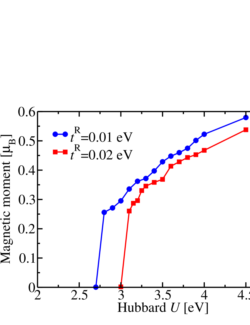
Figure 1: Dependence of the magnetic moment on the Hubbard parameter $U$ at temperature $T=23$ K. Two values of SOI strength are considered: $t^{\rm R}=0.01$ eV (blue circles) and $t^{\rm R}=0.02$ eV (red squares). The magnetic moment is given in units of the Bohr magneton ($\mu_{\rm B}$).

We consider the Hubbard-Rashba model [38] with the Hamiltonian

$$H =\sum_{<j,l>,s}t^{\phantom{\dagger}}_{jl}c^{\dagger}_{js}c^{\phantom{\dagger}}_{ls}+U\sum_{j}c^{\dagger}_{j\uparrow}c^{\phantom{\dagger}}_{j\uparrow}c^{\dagger}_{j\downarrow}c^{\phantom{\dagger}}_{j\downarrow}$$ (59)

$$+it^{\rm R}\sum_{<j,l>,s,s^{\prime}}\hat{{\bm{e}}}_{z}\cdot({\bm{\sigma}}_{ss^{\prime}}\times{\bm{d}}^{\phantom{\dagger}}_{jl})c^{\dagger}_{js}c^{\phantom{\dagger}}_{ls^{\prime}},$$

where $t^{\phantom{\dagger}}_{jl}$ is the hopping amplitude, $U$ is the strength of the Hubbard interaction, $t^{\rm R}$ quantifies the Rashba-type SOI, and ${\bm{d}}_{jl}=({\bm{R}}_{j}-{\bm{R}}_{l})/a$ is the distance vector between sites $j$ and $l$, where $a$ is the lattice constant. The notation $<j,l>$ means that $j$ and $l$ are nearest neighbors. We consider a two-dimensional square lattice with lattice translation invariance and $\hat{{\bm{e}}}_{z}$ is a unit vector perpendicular to the lattice.

For this model we give explicit expressions for the moments in Appendix A. The moments needed to evaluate the correlation functions of Sec. III are discussed in Appendix B, while explicit expressions for the moments required for the calculation of the AHE are given in Appendix C.

We set the nearest neighbor hopping to $t^{\phantom{\dagger}}_{jl}=-0.2{\rm eV}\delta_{1,|d_{xjl}|+|d_{yjl}|}$, the site occupation

$$n=n_{\uparrow}+n_{\downarrow}=\langle c^{\dagger}_{i\uparrow}c_{i\uparrow}\rangle+\langle c^{\dagger}_{i\downarrow}c_{i\downarrow}\rangle$$ (60)

to $n=0.675$ and we vary the Hubbard U parameter between 2 eV and 5 eV. We perform calculations for two SOI strengths, $t^{\rm R}=0.01$ eV, and $t^{\rm R}=0.02$ eV. We use an $80\times 80$ $k$-mesh in the calculations.

In Fig. 1 we show the magnetic moment as a function of $U$ at the temperature $T=23$ K. Around $U=2.7$ eV the system becomes ferromagnetic when $t^{\rm R}=0.01$ eV. When SOI is larger, i.e., $t^{\rm R}=0.02$ eV, the onset of ferromagnetism occurs at a higher $U$ of around 3 eV. Therefore, SOI suppresses the onset of ferromagnetism in this system.

In Fig. 2 we show the bandstructure in the nonmagnetic phase at $U=2$ eV. The lower Hubbard bands describe electrons that hop between empty sites, while the upper Hubbard bands describe electrons hopping between sites that are already occupied by an electron. Consequently, the lower and upper Hubbard bands are separated in energy by roughly $U$. Surprisingly, the Rashba splitting is larger for the upper Hubbard bands than for the lower ones. The bandstructure in the ferromagnetic phase at $U=4$ eV is shown in Fig. 3. Both the upper and the lower Hubbard bands are exchange-split, while the effect of Rashba SOI on the bandstructure is not visible directly.

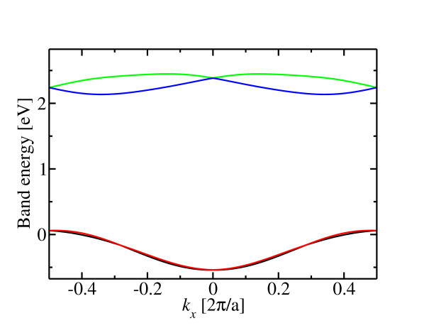
Figure 2: Bandstructure for $U=2$ eV at $T$=23 K when $t^{\rm R}=0.02$ eV. For this value of $U$ the system is non-magnetic. The Rashba splitting is larger for the upper Hubbard bands than for the lower ones.

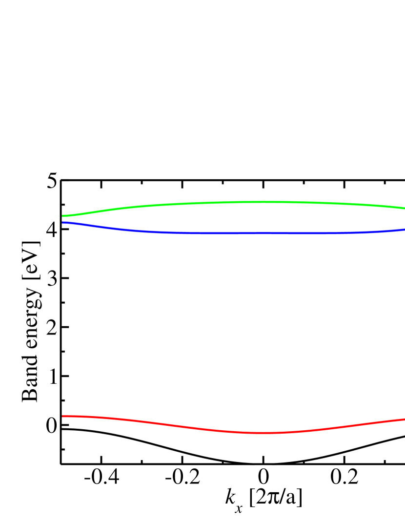
Figure 3: Bandstructure for $U=4$ eV at $T$=23 K when $t^{\rm R}=0.02$ eV. For this value of $U$ the system is ferromagnetic.

In Fig. 4 we show the temperature-dependence of the magnetic moment at $U=4$ eV. The magnetic moment decreases monotonously with temperature. The Curie temperature is smaller when SOI is larger. This is consistent with the finding in Fig. 1 that SOI suppresses ferromagnetism in this system.

In Fig. 5 we show the temperature-dependence of the intrinsic AHE conductivity. Since AHE requires SOI, higher SOI leads to larger AHE. Interestingly, $\sigma_{xy}$ increases with increasing $T$. Phenomenological theory usually assumes that $\sigma_{xy}$ is proportional to the magnetization. However, from zero temperature up to the Curie temperature the magnetic moment decreases, while the AHE conductivity increases according to Fig. 5. This increase of the AHE conductivity with decreasing magnetic moment is therefore surprising at first.

An explanation may be found by recalling in which cases the AHE is predicted to be proportional to the magnetic moment. When the intrinsic AHE is generated predominantly by the term $\propto L_{z}S_{z}$ in the SOI ($L_{z}$ and $S_{z}$ are the orbital and spin angular momentum operators, respectively) and when the magnetic moment is sufficiently small we may argue that the spin-resolved AHE conductivity has opposite sign for spin-up and spin-down electrons, i.e., ${\rm sign}(\sigma^{\uparrow}_{xy})=-{\rm sign}(\sigma^{\downarrow}_{xy})$, because $L_{z}S_{z}=L_{z}$ for spin-up electrons and $L_{z}S_{z}=-L_{z}$ for spin-down electrons. As a consequence, a pure spin-current is generated from the intrinsic spin-Hall effect when the magnetization is zero: $\sigma^{\rm SHE}_{xy}=\sigma^{\uparrow}_{xy}-\sigma^{\downarrow}_{xy}=2\sigma^{\uparrow}_{xy}$. For small magnetic moment the spin-resolved AHE conductivities do not satisfy $\sigma^{\uparrow}_{xy}=-\sigma^{\downarrow}_{xy}$ any more [40] and it is plausible to assume that both depend linearly on the magnetization $M$ in the leading orders,

$$\sigma^{s}_{xy}(M)=s\sigma^{(0)}_{xy}+\left.\frac{\partial\sigma^{(0)}_{xy}}{\partial M}\right|_{M=0}M,$$ (61)

where $s=1$ for spin-up and $s=-1$ for spin-down. This yields

$$\sigma^{\rm SHE}_{xy}(M)=\sigma^{\uparrow}_{xy}(M)-\sigma^{\downarrow}_{xy}(M)=2\sigma^{(0)}_{xy},$$ (62)

$$\sigma^{\rm AHE}_{xy}(M)=\sigma^{\uparrow}_{xy}(M)+\sigma^{\downarrow}_{xy}(M)=2\left.\frac{\partial\sigma^{(0)}_{xy}}{\partial M}\right|_{M=0}M.$$

Thus, one may expect $\sigma^{\rm AHE}_{xy}(M)\propto M$ when only the term $L_{z}S_{z}$ from SOI is relevant. However, this is often not the case, i.e., spin-flip transitions may be important for the AHE [41].

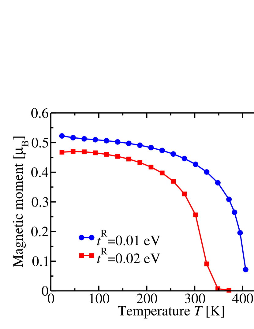
Figure 4: Temperature-dependence of the magnetic moment at $U=4$ eV for SOI-strength $t^{\rm R}=0.01$ eV (circles) and $t^{\rm R}=0.02$ eV (squares). Stronger SOI suppresses the Curie temperature.

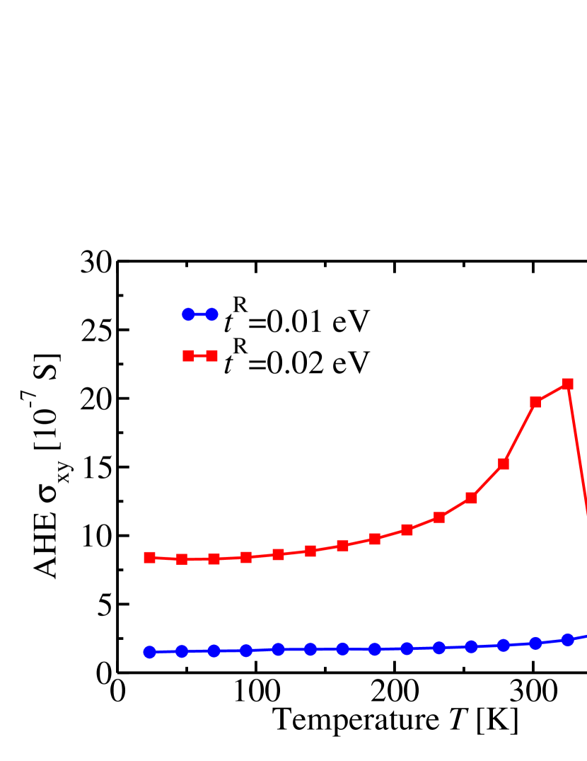
Figure 5: Temperature-dependence of the intrinsic AHE conductivity at $U=4$ eV.

In fact the Rashba SOI does not contain any term that preserves the spin $S_{z}$, i.e., in the language of Ref. [41] it generates only spin-flip transitions. However, when all virtual transitions that give rise to the AHE are of spin-flip type, there is no reason for Eq. (61) to be valid. The spin-flip transitions occur between up- and down-states, and their energy difference decreases when the magnetic moment decreases. Therefore, the spin-flip transitions become more important in Eq. (58) when the energy denominator decreases due to the decrease of the magnetization.

To verify this hypothesis we investigate the dependence of the AHE conductivity on the Hubbard parameter U at a fixed small temperature of $T=23$ K. Thereby we modify the magnetic moment without changing the temperature. The result is shown in Fig. 6. Indeed $\sigma_{xy}$ increases when lowering $U$ from 4.5 eV down to 2.8 eV. Therefore, the dominant mechanism for the strong increase of $\sigma_{xy}$ with increasing temperature in Fig. 5 is indeed the decrease of the magnetic moment.

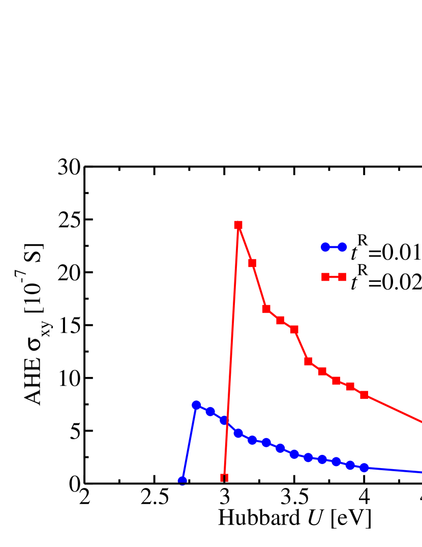
Figure 6: Dependence of the intrinsic AHE conductivity on Hubbard U at $T=23$ K.

VI Outlook

In order to judge if the selfconsistent spectral moment method may replace LDA+$U$ while keeping the computational effort low, we briefly discuss the differences to LDA+$U$. The orbital-resolved occupation matrix, which needs to be computed self-consistently in LDA+$U$ calculations for all atomic orbitals for which correlations are included, corresponds to the correlator $\langle c^{\dagger}_{i\alpha}c_{j\beta}\rangle$ in the self-consistent moment method. In LDA+$U$ only the on-site elements are considered, i.e., only $\langle c^{\dagger}_{0\alpha}c_{0\beta}\rangle$. However, including the nearest neighbors will often not pose problems. Clearly, the matrix structure of $\langle c^{\dagger}_{i\alpha}c_{j\beta}\rangle$ resembles the one of the hopping matrix elements, i.e., the matrix elements of the Hamiltonian between Wannier functions [29]. Therefore, for all systems where the calculation of the hopping matrix does not pose problems, e.g. computer memory issues, we do not anticipate issues concerning the correlator $\langle c^{\dagger}_{i\alpha}c_{j\beta}\rangle$.

The higher-order correlators of the type $\langle c^{\dagger}_{i\alpha}c^{\dagger}_{j\beta}c_{l\gamma}c_{m\delta}\rangle$ are often only needed for special cases such as $i=j$ and $l=m$. Therefore, while the most general form $\langle c^{\dagger}_{i\alpha}c^{\dagger}_{j\beta}c_{l\gamma}c_{m\delta}\rangle$ has 4 independent site indices, $i,j,l,m$, it will often be sufficient to compute it only with one site index. Moreover, when we consider only on-site Coulomb interactions, similar to standard LDA+$U$, the range of the orbital indices $\alpha,\beta,\gamma,\delta$ can be restricted significantly. Thus, while the number of basis functions in LDA calculations based on FLAPW increases proportionally to the system volume, leading to a quadratic increase of the memory requirement of the Hamiltonian with system volume, we expect that the computer memory needed to hold $\langle c^{\dagger}_{i\alpha}c^{\dagger}_{j\beta}c_{l\gamma}c_{m\delta}\rangle$ scales only proportionally to the number of correlated atoms in the system, i.e., often proportionally to the volume and not to the square of the volume. This is similar to the scaling of the orbital-resolved occupation matrix with system size in LDA+$U$, which is proportional to the number of correlated atoms.

Thus, while in LDA+$U$ one needs to compute the orbital-resolved occupation matrix for all correlated atoms, in the selfconsistent spectral moment method one has to compute several correlators of the type $\langle c^{\dagger}_{i\alpha}c_{j\beta}\rangle$ and $\langle c^{\dagger}_{i\alpha}c^{\dagger}_{j\beta}c_{l\gamma}c_{m\delta}\rangle$. Since their structure and memory requirement is similar to the one of matrix elements computed for Wannier interpolation [29, 20, 21], we expect that this is feasible for a large range of realistic materials without a dramatic increase of the computer time or memory requirements, because experience with Wannier functions suggests that the calculation of such matrix elements is much faster than the duration of the LDA selfconsistency cycle if only orbitals for the occupied and first few unoccupied states are considered. In contrast, a recent comparative study of several electronic structure codes estimated that eDMFT takes 5000 times more computer time than meta-GGA with the modified Becke-Johnson potential [42].

Finally, in LDA+$U$ the orbital-resolved occupation matrix is used to compute the potential matrix, which is employed to supplement the Hamiltonian by correlation effects. This step may be performed as a second variation step, i.e., one may first compute the LDA eigenvalues and eigenfunctions in first variation, followed by the calculation of the LDA+$U$ eigenvalues and eigenfunctions in second variation [43]. Similarly, in the selfconsistent moment method one may first compute the LDA eigenvalues and eigenfunctions in first variation, followed by the construction of the spectral function from the first four moment matrices in second variation. This second variation approach is expected to take only a fraction of the computing time of the first variation step.

In comparison to LDA+DMFT, one drawback of the selfconsistent moment method is that it does not give access to the imaginary part of the selfenergy. However, since the selfconsistent moment method has been used before successfully to study finite-temperature magnetism [22, 23, 24], we do not expect this to be a major drawback for this application. Moreover, many response properties of interest in spintronics are not strongly dependent on the electron correlation selfenergy in a large range of realistic materials, because they are at most sensitive to the electron lifetime at the Fermi surface, which is often determined by scattering rather than electron correlation effects. In such cases, the transfer of spectral weight between states of different energy might be more important for the accurate computation of the response function than the imaginary part of the selfenergy. For example, already simple band shifts due to electron correlation effects may sometimes improve the agreement of AHE to experiment [44]. Concerning the description of magnetism at finite temperatures LDA+DMFT studies suggest that missing long wavelength spin waves may lead to an overestimation of the Curie temperature in some cases [5]. We suspect that the selfconsistent moment method suffers from a similar problem whenever the smallest possible magnetic unit cell is chosen and when translational invariance is thus enforced.

In comparison to LDA+$U$ the selfconsistent spectral moment method is not only expected to improve the description of magnetism at finite temperatures, but additionally it is expected to capture spectral features that arise from the splitting of bands into lower and upper Hubbard bands, similarly to LDA+DMFT. For example, it has been shown [23] to reproduce the valence band satellite in Ni.

VII Summary

We show that for a general crystal lattice Hamiltonian which describes $N_{\rm W}$ electronic orbitals and which includes the Coulomb interaction the spectral function may be found within an approximation that assumes that the electronic structure is given in terms of $2N_{\rm W}$ bands and $2N_{\rm W}$ spectral weight factors – $N_{\rm W}$ band energies and spectral weights describe the lower Hubbard bands, while $N_{\rm W}$ band energies and spectral weights describe the upper Hubbard bands. For this purpose we generalize the standard two-pole approximation of the selfconsistent moment method to the case of many bands. We argue that the problem of constructing $2N_{\rm W}$ bands and $2N_{\rm W}$ spectral weights from four $N_{\rm W}\times N_{\rm W}$ spectral moment matrices may be considered as a generalization of the well-known problem of finding the $N_{\rm W}$ eigenstates of an $N_{\rm W}\times N_{\rm W}$ single-particle Hamiltonian matrix of a closed quantum system. We describe how the higher correlation functions of the type $\langle c^{\dagger}_{i\alpha}c^{\dagger}_{j\beta}c_{l\gamma}c_{m\delta}\rangle$ may be obtained consistently within this approach by employing the state vectors and state energies of the single particle spectral function. Moreover, we discuss how the response functions may be computed. We present applications of this approach to the Hubbard-Rashba model. Our findings suggest that the many-band spectral-moment method may replace the standard LDA+$U$ approach to correlated electrons when the temperature dependence of the electronic structure or of the response functions needs to be determined. We propose that the many-band spectral-moment method may also be used instead of Hartree-Fock in exploratory model calculations of phase diagrams in the search of new quantum states that arise from the interplay of SOI and correlation effects.

Appendix A Spectral Moments in the Hubbard-Rashba model

In this section we give explicit expressions for the moments Eq. (2) of the single-particle spectral function evaluated for the Hubbard-Rashba model introduced in Eq. (59). The zeroth moment is given by

$$\tilde{M}^{(0)}_{{\bm{k}}ss^{\prime}}=\frac{1}{N}\sum_{lj}e^{i{\bm{k}}\cdot({\bm{R}}_{l}-{\bm{R}}_{j})}\langle[c_{ls},c^{\dagger}_{js^{\prime}}]_{+}\rangle=\delta_{ss^{\prime}},$$ (63)

where $s,s^{\prime}=\uparrow,\downarrow$.

The spin-diagonal first moments are given by

$$\tilde{M}^{(1)}_{{\bm{k}}ss}=\frac{1}{N}\sum_{lj}e^{i{\bm{k}}\cdot({\bm{R}}_{l}-{\bm{R}}_{j})}\langle[[c_{ls},\mathcal{H}]_{-},c^{\dagger}_{js}]_{+}\rangle$$ (64)

$$=(\epsilon({\bm{k}})-\mu)+U\langle n_{-s}\rangle$$

while those that couple opposite spins are

$$\tilde{M}^{(1)}_{{\bm{k}}s,-s}=\frac{1}{N}\sum_{lj}e^{i{\bm{k}}\cdot({\bm{R}}_{l}-{\bm{R}}_{j})}\langle[[c_{ls},\mathcal{H}]_{-},c^{\dagger}_{j,-s}]_{+}\rangle$$ (65)

$$={\rm Re}[\alpha({\bm{k}})]-si{\rm Im}[\alpha({\bm{k}})]-\frac{U}{N}\sum_{l}\langle c^{\dagger}_{l,-s}c_{ls}\rangle.$$

Here, we defined

$$\alpha({\bm{k}})=\frac{1}{N}t^{\rm R}\sum_{<j,l>}e^{i{\bm{k}}\cdot({\bm{R}}_{j}-{\bm{R}}_{l})}[d_{xjl}+id_{yjl}],$$ (66)

where $d_{xjl}$ and $d_{yjl}$ are the $x$ and $y$ components, respectively, of the distance vector ${\bm{d}}_{jl}$ used in the Rashba-type SOI in Eq. (59).

For equal spins the second moments are

$$\tilde{M}^{(2)}_{{\bm{k}}ss}=\frac{1}{N}\sum_{lj}e^{i{\bm{k}}\cdot({\bm{R}}_{l}-{\bm{R}}_{j})}\langle[[c_{ls},\mathcal{H}]_{-},[\mathcal{H},c^{\dagger}_{js}]_{-}]_{+}\rangle$$ (67)

$$=(\epsilon({\bm{k}})-\mu)^{2}+2U\langle n_{-s}\rangle(\epsilon({\bm{k}})-\mu)+U^{2}\langle n_{-s}\rangle$$

$$-2U{\rm Re}\left[\alpha({\bm{k}})\frac{1}{N}\sum_{l}\langle c^{\dagger}_{l\downarrow}c_{l\uparrow}\rangle\right]+|\alpha({\bm{k}})|^{2},$$

while they are

$$\tilde{M}^{(2)}_{{\bm{k}}s-s}=\frac{1}{N}\sum_{lj}e^{i{\bm{k}}\cdot({\bm{R}}_{l}-{\bm{R}}_{j})}\langle[[c_{ls},\mathcal{H}]_{-},[\mathcal{H},c^{\dagger}_{j,-s}]]_{+}\rangle$$ (68)

$$=[2\epsilon({\bm{k}})-2\mu+nU][{\rm Re}[\alpha({\bm{k}})]-si{\rm Im}[\alpha({\bm{k}})]]$$

$$-[U^{2}+2U(\epsilon({\bm{k}})-\mu)]\frac{1}{N}\sum_{l}\langle c^{\dagger}_{l,-s}c_{ls}\rangle$$

for opposite spins.

The third moments are

$$\tilde{M}^{(3)}_{{\bm{k}}ss}=\frac{1}{N}\sum_{lj}e^{i{\bm{k}}\cdot({\bm{R}}_{l}-{\bm{R}}_{j})}\langle[[[c_{ls},\mathcal{H}]_{-},\mathcal{H}]_{-},[\mathcal{H},c^{\dagger}_{js}]_{-}]_{+}\rangle$$ (69)

$$=[\epsilon({\bm{k}})-\mu]^{3}+3U\langle n_{-s}\rangle[\epsilon({\bm{k}})-\mu]^{2}-3U^{2}\langle n_{-s}\rangle\mu$$

$$+2U^{2}\epsilon({\bm{k}})n_{-s}+2U^{2}t_{00}n_{-s}+U^{3}n_{-s}$$

$$-U^{2}\frac{1}{N}\sum_{lj}e^{i{\bm{k}}\cdot({\bm{R}}_{l}-{\bm{R}}_{j})}t_{lj}\langle c^{\dagger}_{l,-s}c^{\dagger}_{j,-s}c_{l,-s}c_{j,-s}\rangle$$

$$+U^{2}\frac{1}{N}\sum_{lj}t_{lj}\langle(2n_{ls}-1)c^{\dagger}_{l,-s}c_{j,-s}\rangle$$

$$+U^{2}\frac{1}{N}\sum_{lj}e^{i{\bm{k}}\cdot({\bm{R}}_{l}-{\bm{R}}_{j})}t_{lj}\langle c^{\dagger}_{js}c^{\dagger}_{l,-s}c_{ls}c_{j,-s}\rangle$$

$$+U^{2}\frac{1}{N}\sum_{lj}e^{i{\bm{k}}\cdot({\bm{R}}_{l}-{\bm{R}}_{j})}t_{lj}\langle c^{\dagger}_{js}c^{\dagger}_{j,-s}c_{ls}c_{l,-s}\rangle$$

$$+U^{2}\frac{2}{N}\sum_{l}{\rm Re}\left[\alpha({\bm{k}})\langle c^{\dagger}_{l,-s}c_{l,s}\rangle\right]$$

$$+3|\alpha({\bm{k}})|^{2}[\epsilon({\bm{k}})-\mu]+|\alpha({\bm{k}})|^{2}U(n+n_{-s})$$

$$+6U[\epsilon({\bm{k}})-\mu]{\rm Re}\left[\alpha({\bm{k}})\frac{1}{N}\sum_{l}\langle c^{\dagger}_{l,-s}c_{ls}\rangle\right]$$

$$+U^{2}\frac{2}{N}\sum_{lj}{\rm Re}\left[e^{i{\bm{k}}\cdot({\bm{R}}_{l}-{\bm{R}}_{j})}\alpha_{lj}\langle c^{\dagger}_{l,-s}c^{\dagger}_{j,-s}c_{ls}c_{j,-s}\rangle\right],$$

when the spins are parallel, and

$$\tilde{M}^{(3)}_{{\bm{k}}\uparrow\downarrow}=\frac{1}{N}\sum_{lj}e^{i{\bm{k}}\cdot({\bm{R}}_{l}-{\bm{R}}_{j})}\langle[[[c_{l\uparrow},\mathcal{H}]_{-},\mathcal{H}]_{-},[\mathcal{H},c^{\dagger}_{j\downarrow}]]_{+}\rangle$$ (70)

$$=-3[\alpha({\bm{k}})]^{*}[\epsilon({\bm{k}})-\mu]^{2}-[\alpha({\bm{k}})]^{*}|\alpha({\bm{k}})|^{2}-U^{2}[\alpha({\bm{k}})]^{*}n$$

$$-\left(3[\epsilon({\bm{k}})-\mu]^{2}+2|\alpha({\bm{k}})|^{2}+2U[\epsilon({\bm{k}})-\mu]\right)\frac{U}{N}\sum_{l}\langle c^{\dagger}_{l\downarrow}c_{l\uparrow}\rangle$$

$$+U^{2}\frac{1}{N}\sum_{lj}t_{lj}\langle c^{\dagger}_{l\downarrow}c_{j\uparrow}\rangle$$

$$-U\left[\alpha^{*}({\bm{k}})\right]^{2}\frac{1}{N}\sum_{l}\langle c^{\dagger}_{l\uparrow}c_{l\downarrow}\rangle$$

$$-3U[\alpha({\bm{k}})]^{*}[\epsilon({\bm{k}})-\mu]n$$

$$-\left[U^{3}-U^{2}\mu+2U^{2}t_{00}\right]\frac{1}{N}\sum_{l}\langle c^{\dagger}_{l\downarrow}c_{l\uparrow}\rangle$$

$$-U^{2}\frac{1}{N}\sum_{lj}e^{i{\bm{k}}\cdot({\bm{R}}_{l}-{\bm{R}}_{j})}t_{lj}\langle c^{\dagger}_{j\uparrow}c^{\dagger}_{l\downarrow}c_{l\uparrow}c_{j\uparrow}\rangle$$

$$-U^{2}\frac{1}{N}\sum_{lj}e^{i{\bm{k}}\cdot({\bm{R}}_{l}-{\bm{R}}_{j})}t_{lj}\langle c^{\dagger}_{l\downarrow}c^{\dagger}_{j\downarrow}c_{j\uparrow}c_{l\downarrow}\rangle$$

$$+U^{2}\frac{1}{N}\sum_{lj}e^{i{\bm{k}}\cdot({\bm{R}}_{l}-{\bm{R}}_{j})}\alpha^{*}_{lj}\langle c^{\dagger}_{j\uparrow}c^{\dagger}_{l\downarrow}c_{j\uparrow}c_{l\downarrow}\rangle$$

$$-U^{2}\frac{1}{N}\sum_{lj}e^{i{\bm{k}}\cdot({\bm{R}}_{l}-{\bm{R}}_{j})}\alpha^{*}_{lj}\langle c^{\dagger}_{j\uparrow}c^{\dagger}_{j\downarrow}c_{l\uparrow}c_{l\downarrow}\rangle$$

$$-U^{2}\frac{1}{N}\sum_{lj}e^{i{\bm{k}}\cdot({\bm{R}}_{l}-{\bm{R}}_{j})}\alpha_{lj}\langle c^{\dagger}_{l\downarrow}c^{\dagger}_{j\downarrow}c_{l\uparrow}c_{j\uparrow}\rangle$$

$$+U^{2}\frac{1}{N}\sum_{lj}t_{lj}\langle c^{\dagger}_{l\uparrow}c^{\dagger}_{l\downarrow}c_{l\uparrow}c_{j\uparrow}\rangle$$

$$-U^{2}\frac{1}{N}\sum_{lj}t_{lj}\langle c^{\dagger}_{l\downarrow}c^{\dagger}_{j\downarrow}c_{l\uparrow}c_{l\downarrow}\rangle$$

when they are opposite. Here, we defined

$$\alpha_{jl}=[d_{xjl}+id_{yjl}].$$ (71)

The correlation functions of the type $\langle c^{\dagger}_{i\alpha}c^{\dagger}_{j\beta}c_{l\gamma}c_{m\delta}\rangle$ in the expressions of the third moments may be obtained from the spectral theorem in Eq. (15) and Fourier transformation.

Appendix B Correlation functions in the Hubbard-Rashba model

In this appendix we provide examples for explicit expressions of the moments $\tilde{K}^{(0)}_{l\gamma m\delta j\beta{\bm{k}}\alpha}$ and $\tilde{K}^{(1)}_{l\gamma m\delta j\beta{\bm{k}}\alpha}$ used in Sec. III. The zeroth moment is explicitly given by

$$\tilde{K}^{(0)}_{l\gamma m\delta j\beta{\bm{k}}\alpha}=\langle[c^{\dagger}_{j\beta}c_{l\gamma}c_{m\delta},c^{\dagger}_{{\bm{k}}\alpha}]_{+}\rangle$$ (72)

$$=\frac{1}{\sqrt{N}}\left[\langle c^{\dagger}_{j\beta}c_{l\gamma}\rangle e^{-i{\bm{k}}\cdot{\bm{R}}_{m}}\delta_{\alpha\delta}-\langle c^{\dagger}_{j\beta}c_{m\delta}\rangle e^{-i{\bm{k}}\cdot{\bm{R}}_{l}}\delta_{\alpha\gamma}\right].$$

The thermal averages $\langle c^{\dagger}_{j\beta}c_{l\gamma}\rangle$ and $\langle c^{\dagger}_{j\beta}c_{m\delta}\rangle$ in this expression may be obtained from the spectral theorem Eq. (14).

The explicit expression for the first moment

$$\tilde{K}^{(1)}_{l\gamma m\delta j\beta{\bm{k}}\alpha}=\langle[c^{\dagger}_{j\beta}c_{l\gamma}c_{m\delta},[\mathcal{H},c^{\dagger}_{{\bm{k}}\alpha}]_{-}]_{+}\rangle$$ (73)

depends on the Hamiltonian $H$. We list some examples for $\tilde{K}^{(1)}_{l\gamma m\delta j\beta{\bm{k}}\alpha}$ that we obtain for the Hubbard-Rashba model discussed in Sec. V. From

$$\langle[c^{\dagger}_{i\downarrow}c_{i\uparrow}c_{j\downarrow},[H,c^{\dagger}_{l\uparrow}]_{-}]_{+}\rangle=$$ (74)

$$-t_{il}\langle c^{\dagger}_{i\downarrow}c_{j\downarrow}\rangle+\alpha_{jl}\langle c^{\dagger}_{i\downarrow}c_{i\uparrow}\rangle-U\delta_{il}\delta_{lj}\langle c^{\dagger}_{l\downarrow}c_{l\downarrow}\rangle$$

$$+U\delta_{il}\langle c^{\dagger}_{l\uparrow}c^{\dagger}_{l\downarrow}c_{l\uparrow}c_{j\downarrow}\rangle+U\delta_{lj}\langle c^{\dagger}_{i\downarrow}c^{\dagger}_{l\uparrow}c_{i\uparrow}c_{l\downarrow}\rangle$$

we obtain $\tilde{K}^{(1)}_{i\uparrow j\downarrow i\downarrow{\bm{k}}\uparrow}$ by performing a Fourier transformation from the site ${\bm{R}}_{l}$ to the ${\bm{k}}$-point ${\bm{k}}$. As explained in Sec. III this moment is required in order to compute the thermal average $\langle c^{\dagger}_{l\uparrow}c^{\dagger}_{i\downarrow}c_{i\uparrow}c_{j\downarrow}\rangle$. However, according to Eq. (74) additional correlation functions are needed, namely $\langle c^{\dagger}_{l\uparrow}c^{\dagger}_{l\downarrow}c_{l\uparrow}c_{j\downarrow}\rangle$ and $\langle c^{\dagger}_{i\downarrow}c^{\dagger}_{l\uparrow}c_{i\uparrow}c_{l\downarrow}\rangle$. As explained in Sec. III we therefore use a self-consistent procedure that determines all necessary correlation functions $\langle c^{\dagger}_{i\alpha}c^{\dagger}_{j\beta}c_{l\gamma}c_{m\delta}\rangle$.

The correlation function $\langle c^{\dagger}_{l\uparrow}c^{\dagger}_{i\downarrow}c_{j\uparrow}c_{i\uparrow}\rangle$ vanishes without SOI when the spin-quantization axis is chosen to be along the $z$-direction, but it may be non-zero in general when SOI is present. We obtain the corresponding first moment $\tilde{K}^{(1)}_{j\uparrow i\uparrow i\downarrow{\bm{k}}\uparrow}$ from

$$\langle[c^{\dagger}_{i\downarrow}c_{j\uparrow}c_{i\uparrow},[H,c^{\dagger}_{l\uparrow}]_{-}]_{+}\rangle=t_{il}\langle c^{\dagger}_{i\downarrow}c_{j\uparrow}\rangle-t_{jl}\langle c^{\dagger}_{i\downarrow}c_{i\uparrow}\rangle$$ (75)

$$+U\delta_{jl}\langle c^{\dagger}_{i\downarrow}c^{\dagger}_{l\downarrow}c_{i\uparrow}c_{l\downarrow}\rangle-U\delta_{il}\langle c^{\dagger}_{l\uparrow}c^{\dagger}_{l\downarrow}c_{l\uparrow}c_{j\uparrow}\rangle$$

by performing a Fourier transformation from the site ${\bm{R}}_{l}$ to the ${\bm{k}}$-point ${\bm{k}}$.

Appendix C First moments for response functions

In the following we give a few examples for explicit expressions of the first moment of the commutator spectral function obtained by evaluating Eq. (34) for the Hubbard-Rashba model:

$$\tilde{D}^{(1)}_{{\bm{k}}\uparrow\uparrow\uparrow\uparrow}=[\alpha({\bm{k}})]^{*}\langle c^{\dagger}_{0\downarrow}c_{0\uparrow}\rangle+\alpha({\bm{k}})\langle c^{\dagger}_{0\uparrow}c_{0\downarrow}\rangle$$ (76)

$$+U\sum_{j}e^{-i{\bm{k}}\cdot[{\bm{R}}_{j}-{\bm{R}}_{0}]}\langle c^{\dagger}_{0\uparrow}c^{\dagger}_{0\downarrow}c_{j\uparrow}c_{0\downarrow}\rangle$$

$$+U\sum_{j}e^{i{\bm{k}}\cdot[{\bm{R}}_{j}-{\bm{R}}_{0}]}\langle c^{\dagger}_{j\uparrow}c^{\dagger}_{0\downarrow}c_{0\uparrow}c_{0\downarrow}\rangle$$

$$-2\frac{U}{N}\sum_{j,l}e^{i{\bm{k}}\cdot[{\bm{R}}_{j}-{\bm{R}}_{l}]}\langle c^{\dagger}_{j\uparrow}c^{\dagger}_{0\downarrow}c_{l\uparrow}c_{0\downarrow}\rangle$$

and

$$\tilde{D}^{(1)}_{{\bm{k}}\uparrow\downarrow\downarrow\uparrow}=2\alpha({\bm{k}})\langle c^{\dagger}_{0\downarrow}c_{0\uparrow}\rangle$$ (77)

$$+U\sum_{j}e^{-i{\bm{k}}\cdot[{\bm{R}}_{j}-{\bm{R}}_{0}]}\langle c^{\dagger}_{0\uparrow}c^{\dagger}_{0\downarrow}c_{j\uparrow}c_{0\downarrow}\rangle$$

$$+\frac{U}{N}\sum_{j,l}e^{i{\bm{k}}\cdot[{\bm{R}}_{j}-{\bm{R}}_{l}]}\langle c^{\dagger}_{j\uparrow}c^{\dagger}_{0\uparrow}c_{0\uparrow}c_{l\uparrow}\rangle$$

$$+U\sum_{j}e^{i{\bm{k}}\cdot[{\bm{R}}_{j}-{\bm{R}}_{0}]}\langle c^{\dagger}_{0\uparrow}c^{\dagger}_{j\downarrow}c_{0\uparrow}c_{0\downarrow}\rangle$$

$$-\frac{U}{N}\sum_{j,l}e^{i{\bm{k}}\cdot[-{\bm{R}}_{j}-{\bm{R}}_{l}]}\langle c^{\dagger}_{0\uparrow}c^{\dagger}_{0\uparrow}c_{j\uparrow}c_{l\uparrow}\rangle$$

$$-\frac{U}{N}\sum_{j,l}e^{i{\bm{k}}\cdot[{\bm{R}}_{j}-{\bm{R}}_{l}]}\langle c^{\dagger}_{0\downarrow}c^{\dagger}_{j\downarrow}c_{0\downarrow}c_{l\downarrow}\rangle$$

$$-\frac{U}{N}\sum_{j,l}e^{i{\bm{k}}\cdot[{\bm{R}}_{j}+{\bm{R}}_{l}]}\langle c^{\dagger}_{j\downarrow}c^{\dagger}_{l\downarrow}c_{0\downarrow}c_{0\downarrow}\rangle.$$

The correlation functions of the type $\langle c^{\dagger}_{i\alpha}c^{\dagger}_{j\beta}c_{l\gamma}c_{m\delta}\rangle$ in these expressions may be obtained from the spectral theorem in Eq. (15) and Fourier transformation.

References

- Himmetoglu et al. [2014] B. Himmetoglu, A. Floris, S. de Gironcoli, and M. Cococcioni, Hubbard-corrected dft energy functionals: The lda+u description of correlated systems, International Journal of Quantum Chemistry 114, 14 (2014).
- Anisimov et al. [1991] V. I. Anisimov, J. Zaanen, and O. K. Andersen, Band theory and mott insulators: Hubbard u instead of stoner i, Phys. Rev. B 44, 943 (1991).
- Anisimov et al. [1993] V. I. Anisimov, I. V. Solovyev, M. A. Korotin, M. T. Czyżyk, and G. A. Sawatzky, Density-functional theory and nio photoemission spectra, Phys. Rev. B 48, 16929 (1993).
- Solovyev et al. [1994] I. V. Solovyev, P. H. Dederichs, and V. I. Anisimov, Corrected atomic limit in the local-density approximation and the electronic structure of d impurities in rb, Phys. Rev. B 50, 16861 (1994).
- Lichtenstein et al. [2001] A. I. Lichtenstein, M. I. Katsnelson, and G. Kotliar, Finite-temperature magnetism of transition metals: An ab initio dynamical mean-field theory, Phys. Rev. Lett. 87, 067205 (2001).
- Schlotter et al. [2018] S. Schlotter, P. Agrawal, and G. S. D. Beach, Temperature dependence of the dzyaloshinskii-moriya interaction in pt/co/cu thin film heterostructures, Applied Physics Letters 113, 092402 (2018).
- Kim et al. [2014] J. Kim, J. Sinha, S. Mitani, M. Hayashi, S. Takahashi, S. Maekawa, M. Yamanouchi, and H. Ohno, Anomalous temperature dependence of current-induced torques in heterostructures with ta-based underlayers, Phys. Rev. B 89, 174424 (2014).
- Qiu et al. [2014] X. Qiu, P. Deorani, K. Narayanapillai, K.-S. Lee, K.-J. Lee, H.-W. Lee, and H. Yang, Angular and temperature dependence of current induced spin-orbit effective fields in ta/cofeb/mgo nanowires, SCIENTIFIC REPORTS 4, 10.1038/srep04491 (2014).
- Freimuth et al. [2021] F. Freimuth, S. Blügel, and Y. Mokrousov, Effect of magnons on the temperature dependence and anisotropy of spin-orbit torque, Phys. Rev. B 104, 094434 (2021).
- Manchon et al. [2019] A. Manchon, J. Železný, I. M. Miron, T. Jungwirth, J. Sinova, A. Thiaville, K. Garello, and P. Gambardella, Current-induced spin-orbit torques in ferromagnetic and antiferromagnetic systems, Rev. Mod. Phys. 91, 035004 (2019).
- Wang et al. [2020] W. O. Wang, J. K. Ding, B. Moritz, E. W. Huang, and T. P. Devereaux, Dc hall coefficient of the strongly correlated hubbard model, npj Quantum Materials 5, 51 (2020).
- Wang et al. [2021] W. O. Wang, J. K. Ding, B. Moritz, Y. Schattner, E. W. Huang, and T. P. Devereaux, Numerical approaches for calculating the low-field dc hall coefficient of the doped hubbard model, Phys. Rev. Research 3, 033033 (2021).
- Auerbach [2019] A. Auerbach, Equilibrium formulae for transverse magnetotransport of strongly correlated metals, Phys. Rev. B 99, 115115 (2019).
- Auerbach [2018] A. Auerbach, Hall number of strongly correlated metals, Phys. Rev. Lett. 121, 066601 (2018).
- Rózsa et al. [2017] L. Rózsa, U. Atxitia, and U. Nowak, Temperature scaling of the dzyaloshinsky-moriya interaction in the spin wave spectrum, Phys. Rev. B 96, 094436 (2017).
- Callen and Callen [1966] H. Callen and E. Callen, The present status of the temperature dependence of magnetocrystalline anisotropy, and the l(l+1)2 power law, Journal of Physics and Chemistry of Solids 27, 1271 (1966).
- Callen [1963] H. B. Callen, Green function theory of ferromagnetism, Phys. Rev. 130, 890 (1963).
- Yao et al. [2004] Y. Yao, L. Kleinman, A. H. MacDonald, J. Sinova, T. Jungwirth, D.-s. Wang, E. Wang, and Q. Niu, First principles calculation of anomalous hall conductivity in ferromagnetic bcc fe, Phys. Rev. Lett. 92, 037204 (2004).
- Nagaosa et al. [2010] N. Nagaosa, J. Sinova, S. Onoda, A. H. MacDonald, and N. P. Ong, Anomalous hall effect, Rev. Mod. Phys. 82, 1539 (2010).
- Wang et al. [2006] X. Wang, J. R. Yates, I. Souza, and D. Vanderbilt, Ab initio calculation of the anomalous hall conductivity by wannier interpolation, Phys. Rev. B 74, 195118 (2006).
- Freimuth et al. [2014] F. Freimuth, S. Blügel, and Y. Mokrousov, Spin-orbit torques in co/pt(111) and mn/w(001) magnetic bilayers from first principles, Phys. Rev. B 90, 174423 (2014).
- Nolting et al. [1995] W. Nolting, A. Vega, and T. Fauster, Electronic quasiparticle structure of ferromagnetic bcc iron, Zeitschrift für Physik B Condensed Matter 96, 357 (1995).
- Nolting et al. [1989] W. Nolting, W. Borgiel/, V. Dose, and T. Fauster, Finite-temperature ferromagnetism of nickel, Phys. Rev. B 40, 5015 (1989).
- Borgiel and Nolting [1990] W. Borgiel and W. Nolting, Many body contributions to the electronic structure of nickel, Zeitschrift für Physik B Condensed Matter 78, 241 (1990).
- Crépieux and Bruno [2001] A. Crépieux and P. Bruno, Theory of the anomalous hall effect from the kubo formula and the dirac equation, Phys. Rev. B 64, 014416 (2001).
- Bastin et al. [1971] A. Bastin, C. Lewiner, O. Betbeder-Matibet, and P. Nozières, J. Phys. Chem. Solids 32, 1811 (1971).
- Nolting [1975] W. Nolting, On the connection between electric and magnetic properties of the hubbard model i. electrical conductivity, physica status solidi (b) 70, 505 (1975).
- Geipel and Nolting [1988] G. Geipel and W. Nolting, Ferromagnetism in the strongly correlated hubbard model, Phys. Rev. B 38, 2608 (1988).
- Pizzi et al. [2020] G. Pizzi, V. Vitale, R. Arita, S. Blügel, F. Freimuth, G. Géranton, M. Gibertini, D. Gresch, C. Johnson, T. Koretsune, and et al., Wannier90 as a community code: new features and applications, J. Phys.: Condens. Matter 32, 165902 (2020).
- Anisimov et al. [2007] V. I. Anisimov, A. V. Kozhevnikov, M. A. Korotin, A. V. Lukoyanov, and D. A. Khafizullin, Orbital density functional as a means to restore the discontinuities in the total-energy derivative and the exchange–correlation potential, Journal of Physics: Condensed Matter 19, 106206 (2007).
- Witczak-Krempa et al. [2014] W. Witczak-Krempa, G. Chen, Y. B. Kim, and L. Balents, Correlated quantum phenomena in the strong spin-orbit regime, Annual Review of Condensed Matter Physics 5, 57 (2014), https://doi.org/10.1146/annurev-conmatphys-020911-125138 .
- Bertinshaw et al. [2019] J. Bertinshaw, Y. Kim, G. Khaliullin, and B. Kim, Square lattice iridates, Annual Review of Condensed Matter Physics 10, 315 (2019), https://doi.org/10.1146/annurev-conmatphys-031218-013113 .
- Witczak-Krempa and Kim [2012] W. Witczak-Krempa and Y. B. Kim, Topological and magnetic phases of interacting electrons in the pyrochlore iridates, Phys. Rev. B 85, 045124 (2012).
- Witczak-Krempa et al. [2013] W. Witczak-Krempa, A. Go, and Y. B. Kim, Pyrochlore electrons under pressure, heat, and field: Shedding light on the iridates, Phys. Rev. B 87, 155101 (2013).
- Kennedy et al. [2022] W. Kennedy, S. d. A. S. Júnior, N. C. Costa, and R. R. d. Santos, Magnetism and metal-insulator transitions in the rashba-hubbard model (2022), arXiv:2205.08651 .
- Bercioux and Lucignano [2015] D. Bercioux and P. Lucignano, Quantum transport in rashba spin–orbit materials: a review, Reports on Progress in Physics 78, 106001 (2015).
- Manchon et al. [2015] A. Manchon, H. C. Koo, J. Nitta, S. M. Frolov, and R. A. Duine, New perspectives for Rashba spin–orbit coupling, Nature materials 14, 871 (2015).
- Riera [2013] J. A. Riera, Spin polarization in the hubbard model with rashba spin-orbit coupling on a ladder, Phys. Rev. B 88, 045102 (2013).
- Nolting and Brewer [2009] W. Nolting and W. Brewer, Fundamentals of Many-body Physics: Principles and Methods (Springer Berlin Heidelberg, 2009).
- Zhang et al. [2015] W. Zhang, M. B. Jungfleisch, W. Jiang, Y. Liu, J. E. Pearson, S. G. E. t. Velthuis, A. Hoffmann, F. Freimuth, and Y. Mokrousov, Reduced spin-hall effects from magnetic proximity, Phys. Rev. B 91, 115316 (2015).
- Zhang et al. [2011] H. Zhang, F. Freimuth, S. Blügel, Y. Mokrousov, and I. Souza, Role of spin-flip transitions in the anomalous hall effect of fept alloy, Phys. Rev. Lett. 106, 117202 (2011).
- Mandal et al. [2019] S. Mandal, K. Haule, K. M. Rabe, and D. Vanderbilt, Systematic beyond-dft study of binary transition metal oxides, npj Computational Materials 5, 115 (2019).
- Shick et al. [1999] A. B. Shick, A. I. Liechtenstein, and W. E. Pickett, Implementation of the lda+u method using the full-potential linearized augmented plane-wave basis, Phys. Rev. B 60, 10763 (1999).
- Młyńczak et al. [2022] E. Młyńczak, I. Aguilera, P. Gospodarič, T. Heider, M. Jugovac, G. Zamborlini, J.-P. Hanke, C. Friedrich, Y. Mokrousov, C. Tusche, S. Suga, V. Feyer, S. Blügel, L. Plucinski, and C. M. Schneider, Fe(001) angle-resolved photoemission and intrinsic anomalous hall conductivity in fe seen by different ab initio approaches: Lda and gga versus , Phys. Rev. B 105, 115135 (2022).