Fluctuation contribution to Spin Hall Effect in Superconductors

Abstract

We theoretically study the contribution of superconducting fluctuation to extrinsic spin Hall effects in two- and three-dimensional electron gas and intrinsic spin Hall effects in two-dimensional electron gas with Rashba-type spin-orbit interaction. The Aslamazov-Larkin, Density-of-States, Maki-Thompson terms have logarithmic divergence $\ln\epsilon$ in the limit $\epsilon=(T-T_{\mathrm{c}})/T_{\mathrm{c}}\rightarrow+0$ in two-dimensional systems for both extrinsic and intrinsic spin Hall effects except the Maki-Thompson terms in extrinsic effect, which are proportional to $(\epsilon-\gamma_{\varphi})^{-1}\ln\epsilon$ with a cutoff $\gamma_{\varphi}$ in two-dimensional systems. We found that the fluctuation effects on the extrinsic spin Hall effect have an opposite sign to that in the normal state, while those on the intrinsic spin Hall effect have the same sign.

I Introduction

Spin current has opened a new venue to manipulate condensed matter systems. Spin transport experiments were firstly conducted by Tedrow and Meservey[1], who demonstrated that current flow across a ferromagnet-superconductor interface was spin-polarized. Subsequently, Aronov discussed that spin injection from ferromagnet to nonmagnetic metals could be used to amplify the ESR signals[*[][[JETPLett.$\bm{24}$, 32(1976)].]Aronov1976]. Johnson and Silsbee demonstrated that nonlocal response against the local charge current injection from ferromagnetic metal to nonmagnetic metal could be utilized to measure the spin relaxation time[3]. In the nonlocal response, a major role is played by the propagation of non-conserved spin current over a mesoscopic scale termed a spin diffusion length. In addition to finding efficient ways for spin injection and study of nonlocal response due to spin diffusion, spin-charge conversion (spin Hall effect [4, 5, 6, 7, 8, 9, 10, 11, 12, 13, 14, 15, 16, 17] and spin galvanic effect[18, 19]) is also an important issue in physics of spin transport. The spin Hall effect is categorized into two groups according to the origin, viz, extrinsic spin Hall effect [4, 5, 6] caused by the spin-orbit interaction in the disorder potential and intrinsic spin Hall effect [10, 11] that occurs in a perfect crystal with the electric band structure split by the spin-orbit interaction.

Those issues in spin transport have been addressed not only in normal metals but in superconductors[20]. A theory of spin current injected into superconductors by taking account of charge imbalance and spin imbalance of quasiparticles was developed in 1995[21]. In 2012, Hübler et al. reported spin transport in superconducting Al, over distances of several microns, exceeding the normal-state spin-diffusion length and the charge-imbalance length[22]. Wakamura et al. observed spin-relaxation times in superconducting Nb, which is four times longer than that in the normal state[23]. Wakamura et al. [24] reported, in another paper, inverse spin Hall effect (ISHE), conversion from spin current to charge current in superconductors NbN. Recently, several efficient ways of injection of spin current into superconductors near the transition temperature $T_{\rm c}$ have been discussed theoretically in refs [25, 26] in terms of spin-pumping, spin-Seebeck effect, and strong coupling between spin and energy in spin-splitting quasiparticles[27]. Jeon et al. reported that the conversion efficiency of magnon spin to quasiparticle charge in superconducting Nb via ISHE is enhanced compared with that in the normal state near $T_{\rm c}$ [28, 29]. Enhancement of the ISHE signal was observed even at the temperatures up to twice $T_{\rm c}$[29]. Those experimental results imply the importance of superconducting fluctuation effects on spin transport near $T_{\rm c}$. We note that earlier theoretical studies[7, 30, 31] but one [32] have focused on spin Hall effect in superconductors below $T_{\rm c}$.

Fluctuation effects on transport properties above the superconducting transition temperature $T_{\rm c}$ were firstly studied by Aslamazov and Larkin[33], Maki[34], and Thompson[35] on electric conductivity[36]. Dominant fluctuation processes contributing to electric conductivity are the charge transport by the fluctuating Cooper pairs [33], the reduction of the density of states by the presence of the fluctuating Cooper pairs, and the scattering of electrons by the fluctuation of Cooper pairs. These three processes are represented by the Feynman diagrams, each of which is called the Aslamazov-Larkin(AL) terms, DOS terms, and Maki-Thompson (MT) terms, respectively. The MT terms for electric conductivity contain the anomalous part, which diverges for all temperatures above $T_{\rm c}$ in one- and two-dimensional systems. This anomalous part is cut off by the phase-breaking parameter with various origins such as the paramagnetic impurities, magnetic fields, inelastic phonon scattering, and nonlinear fluctuation effects (See Secs. 8.3.3 and 8.3.4 in [36]). Depending on the phase-breaking parameter, either the AL terms or the MT terms dominantly contribute to electric conductivity. The superconducting fluctuation effect of extrinsic anomalous Hall effects[37], which is closely related to the spin Hall effect, was studied by Li and Levchenko[38]. In the ref. [32], the spin Hall effect in the presence of a magnetic field was studied by consideration of the AL terms cooperating with the Hartree approximation.

In this paper, we discuss the fluctuation effects on the spin Hall effect in superconductors above $T_{\rm c}$ in the absence of magnetic fields with the lowest order processes of the fluctuation propagator. We study the extrinsic spin Hall effect in the two and three-dimensional electron gas by incorporating the superconducting fluctuations in the model used by Tse and Das Sarma[9]. We also investigate the intrinsic spin Hall effect by taking account of the superconducting fluctuations in the model used by Sinova et al. [11] viz, the two-dimensional electron gas with the Rashba spin-orbit interaction.

Our main results are summarized as follows:

• Extrinsic spin Hall effect in two dimensional electron gas [Sec. III]: In the presence of the side jump process, the DOS terms contribute dominantly and suppress the spin Hall conductivity in the normal state. They have a logarithmic divergence $\ln(1/\epsilon)$ in the limit $\epsilon=(T-T_{\mathrm{c}})/T_{\mathrm{c}}\rightarrow+0$. In the presence of the skew scattering process, either the DOS terms or the MT terms contribute dominantly and suppress the spin Hall conductivity in the normal state, depending on the relative ratio between three dimensionless parameters: $\epsilon$, the phase-breaking parameter $\gamma_{\varphi}$, and $T\tau/\hbar$ with the impurity scattering time $\tau$. The DOS terms have the logarithmic divergence $\ln(1/\epsilon)$ while the MT terms are proportional to $(\epsilon-\gamma_{\varphi})^{-1}\ln(1/\epsilon)$. The results are summarized in Tables 1 and 2 in Sec. V.

• Extrinsic spin Hall effect in three-dimensional electron gas [Sec. III]: In the presence of the side jump process, the AL, DOS, and MT terms have no singularity concerning $\epsilon$. The DOS terms contribute dominantly and suppress the spin Hall conductivity in the normal state. In the presence of the skew scattering process, the MT terms are proportional to $(\epsilon^{1/2}+\gamma_{\varphi}^{1/2})^{-1}$ while the AL and DOS terms have no singularity. The MT terms thus contribute dominantly and suppress the spin Hall conductivity in the normal state.

• Intrinsic spin Hall effect in Rashba model [Sec. IV]: The AL, DOS, and MT terms have logarithmic divergence $\ln(1/\epsilon)$ with the coefficients of the same order. The sum of these contributions has the same sign as the spin Hall conductivity in the normal state and enhances the spin Hall conductivity. The results are summarized in Tables 3 in Sec. V.

The rest of the present paper is organized as follows. The next section summarizes the extrinsic and intrinsic spin Hall effect in the normal state and fluctuation propagator. In Sec. III, we address the fluctuation effects on extrinsic spin Hall effects in the presence of side jump and skew scattering processes in two- and three-dimensional electron gas. In Sec. IV, we discuss the fluctuation effects on intrinsic spin Hall effects in two-dimensional electron gas with Rashba spin-orbit interaction. In Sec. V, we discuss singularity near $T_{\rm c}$ and magnitude of fluctuation contribution in AL, DOS, and MT terms. We also raise several issues to be addressed in the future. In Sec. VI, we conclude the present study. We defer the details of derivation in Secs. III and IV to supplemental materials. We list the symbols used in the main text and supplemental materials in the appendix.

Throughout this paper, we set the Boltzmann constant to be unity (i.e., $k_{\rm B}=1$) and take the electric charge of the carriers to be negative ($-e<0$).

II Preliminaries: spin Hall effect in the normal state and fluctuation propagator

This section aims to define the models, fix the notations, and summarize earlier results in the form seamless to the calculation presented in the following sections.

II.1 Extrinsic spin Hall effect

In this section, we summarize the extrinsic spin Hall effect in the two-dimensional and three-dimensional electron gas following [9].

II.1.1 Hamiltonian, Spin current density, and Charge current density

We start with the following single-particle Hamiltonian:

$$H= \frac{(\bm{p}+e\bm{A})^{2}}{2m}-\frac{\lambda_{0}^{2}}{4\hbar}\quantity[\bm{\sigma}\crossproduct\gradient\mathcal{V}(\bm{r})]\dotproduct(\bm{p}+e\bm{A})+\mathcal{V}(\bm{r})$$ (1)

$$\equiv H_{0}+H_{\mathrm{SO}}+\mathcal{V},$$ (2)

which consists of the kinetic energy $H_{0}$, the spin-orbit interaction $H_{\mathrm{SO}}$ and the potential energy due to impurities $\mathcal{V}$. $\mathcal{V}(\bm{r})$ can be written as $\mathcal{V}(\bm{r})=\sum_{i}\mathcal{V}_{\mathrm{single}}(\bm{r}-\bm{R}_{i})$, where $\mathcal{V}_{\mathrm{single}}(\bm{r})$ is a potential energy of single impurity and $\bm{R}_{i}$ is the position of the $i$-th impurity. In Eq. (2), $\bm{A}$ denotes the spatially uniform vector potential. The symbol $\bm{\sigma}={}^{t}(\sigma^{x},\sigma^{y},\sigma^{z})$ denotes the Pauli matrices. The symbol $\lambda_{0}$, which has the dimension of length, is the coupling strength of spin-orbit interaction.

The random average of the impurity potential is given by

$$\begin{aligned} \expectationvalue{\mathcal{V}(\bm{r}_{1})\mathcal{V}(\bm{r}_{2})}=&n_{\rm i}v_{0}^{2}\delta(\bm{r}_{1}-\bm{r}_{2})\\ \expectationvalue{\mathcal{V}(\bm{r}_{1})\mathcal{V}(\bm{r}_{2})\mathcal{V}(\bm{r}_{3})}=&n_{\rm i}v_{0}^{3}\delta(\bm{r}_{1}-\bm{r}_{2})\delta(\bm{r}_{2}-\bm{r}_{3}),\end{aligned}$$ (3)

where $n_{\rm i}$ is the density of impurities and $v_{0}$ is the uniform component of the Fourier transform of $\mathcal{V}_{\mathrm{single}}(\bm{r})$

$$v_{0}=\int d\bm{r}\;\mathcal{V}_{\mathrm{single}}(\bm{r}).$$ (4)

The single-particle charge current is given by

$$\bm{J}_{\rm c}=-e\bm{u}=-e\left(\frac{\bm{p}+e\bm{A}}{m}-\frac{\lambda_{0}^{2}}{4\hbar}\bm{\sigma}\crossproduct\gradient\mathcal{V}\right),$$ (5)

in terms of the velocity $\bm{u}$

$$\bm{u}= \frac{i}{\hbar}\commutator{H}{\bm{r}}=\frac{\bm{p}+e\bm{A}}{m}-\frac{\lambda_{0}^{2}}{4\hbar}\bm{\sigma}\crossproduct\gradient\mathcal{V}.$$ (6)

We define the single-particle spin current by

$$\bm{J}_{\rm s}=-\frac{e}{4}\poissonbracket{\sigma^{z}}{\bm{u}}=-e\quantity(\frac{\bm{p}+e\bm{A}}{2m}\sigma^{z}-\frac{\lambda_{0}^{2}}{8\hbar}\hat{\bm{z}}\crossproduct\gradient{\mathcal{V}}I)\qquad(\text{$I$ is the $2\times 2$ unit matrix}).$$ (7)

Each term in the Hamiltonian Eq. (2) is rewritten in the second quantized form as

$$H_{0}= \sum_{\alpha\bm{k}}\psi_{\bm{k}\alpha}^{\dagger}\frac{1}{2m}\quantity(\hbar\bm{k}+e\bm{A})^{2}\psi_{\bm{k}\alpha}$$ (8)

$$H_{\mathrm{SO}}= -\frac{i\lambda_{0}^{2}}{4V}\sum_{\alpha\beta}\sum_{\bm{k}\bm{k}^{\prime}}\psi_{\bm{k}\alpha}^{\dagger}(\bm{k}\crossproduct\bm{k}^{\prime})\dotproduct\bm{\sigma}_{\alpha\beta}\mathcal{V}_{\bm{k}-\bm{k}^{\prime}}\psi_{\bm{k}^{\prime}\beta}-\frac{ie\lambda_{0}^{2}}{4\hbar V}\sum_{\alpha\beta}\sum_{\bm{k}\bm{k}^{\prime}}((\bm{k}^{\prime}-\bm{k})\crossproduct\bm{\sigma}_{\alpha\beta})\dotproduct\bm{A}\mathcal{V}_{\bm{k}-\bm{k}^{\prime}}\psi_{\bm{k}\alpha}^{\dagger}\psi_{\bm{k}^{\prime}\beta}$$ (9)

$$\mathcal{V}= \frac{1}{V}\sum_{\alpha}\sum_{\bm{k}\bm{k}^{\prime}}\mathcal{V}_{\bm{k}-\bm{k}^{\prime}}\psi_{\bm{k}\alpha}^{\dagger}\psi_{\bm{k}^{\prime}\alpha},$$ (10)

in terms of the creation $\psi^{\dagger}_{\bm{k}\alpha}$ and annihilation $\psi_{\bm{k}\alpha}$ operators of one-particle state with the wavevector $\bm{k}$ and $z$-component of spin $\alpha=\uparrow,\downarrow$. The symbol $V$ denotes the volume of the system.

The spin current density is written in terms of the field operators $\psi_{\alpha}^{\dagger}(\bm{r}),\psi_{\alpha}(\bm{r})$ in the second quantized form as

$$\bm{j}_{\rm s}(\bm{r})= -e\sum_{\alpha\beta}\psi_{\alpha}^{\dagger}(\bm{r})\quantity(\frac{\bm{p}+e\bm{A}}{2m}\sigma^{z}_{\alpha\beta}-\frac{\lambda_{0}^{2}}{8\hbar}\hat{\bm{z}}\crossproduct\gradient V\delta_{\alpha\beta})\psi_{\beta}(\bm{r})$$ (11)

and the uniform component of the Fourier transform of Eq. (11), which we denote by $\bm{j}_{\rm s}$, is written as

$$\bm{j}_{\mathrm{s}}= -\frac{e}{2}\sum_{\alpha\beta}\sum_{\bm{k}\bm{k}^{\prime}}\psi_{\bm{k}\alpha}^{\dagger}\quantity[\frac{\hbar\bm{k}}{m}\sigma_{\alpha\beta}^{z}\delta_{\bm{k}\bm{k}^{\prime}}-\frac{i\lambda_{0}^{2}}{4\hbar V}\hat{\bm{z}}\delta_{\alpha\beta}\crossproduct(\bm{k}-\bm{k}^{\prime})\mathcal{V}_{\bm{k}-\bm{k}^{\prime}}+\frac{e}{m}\bm{A}\sigma_{\alpha\beta}^{z}\delta_{\bm{k}\bm{k}^{\prime}}]\psi_{\bm{k}^{\prime}\beta}$$ (12)

$$\equiv \bm{j}_{\mathrm{s}}^{(1)}+\bm{j}_{\mathrm{s}}^{(2)}+\bm{j}_{\mathrm{s}}^{(3)}.$$ (13)

The charge current density is written in the second quantized form as

$$\bm{j}_{\rm c}(\bm{r})=-e\sum_{\alpha}\psi_{\alpha}^{\dagger}(\bm{r})\left(\frac{\bm{p}+e\bm{A}}{m}\right)\psi_{\alpha}(\bm{r})+\frac{e\lambda_{0}^{2}}{4\hbar}\sum_{\alpha\beta}\bm{\sigma}_{\alpha\beta}\crossproduct\gradient\mathcal{V}(\bm{r})\psi_{\alpha}^{\dagger}(\bm{r})\psi_{\beta}(\bm{r}).$$ (14)

The uniform component of the Fourier transform of charge current density, which we denote by $\bm{j}_{\rm c}$, is given by

$$\bm{j}_{\mathrm{c}}= -e\sum_{\alpha\beta}\sum_{\bm{k}\bm{k}^{\prime}}\psi_{\bm{k}\alpha}^{\dagger}\quantity[\frac{\hbar\bm{k}}{m}\delta_{\alpha\beta}\delta_{\bm{k}\bm{k}^{\prime}}-\frac{i\lambda_{0}^{2}}{4\hbar V}\bm{\sigma}_{\alpha\beta}\crossproduct(\bm{k}-\bm{k}^{\prime})\mathcal{V}_{\bm{k}-\bm{k}^{\prime}}+\frac{e}{m}\bm{A}\delta_{\alpha\beta}\delta_{\bm{k}\bm{k}^{\prime}}]\psi_{\bm{k}^{\prime}\beta}$$ (15)

$$\equiv \bm{j}_{\mathrm{c}}^{(1)}+\bm{j}_{\mathrm{c}}^{(2)}+\bm{j}_{\mathrm{c}}^{(3)}.$$ (16)

II.1.2 Spin Hall conductivity

We consider the spin current density against the uniform electric field with the use of the Kubo formula. The random average of the impurity potential Eq. (3) becomes

$$\expectationvalue{\mathcal{V}_{\bm{k}}\mathcal{V}_{\bm{k}^{\prime}}}= n_{\rm i}v_{0}^{2}V\delta_{\bm{k}+\bm{k}^{\prime},0}$$ (17)

and

$$\expectationvalue{\mathcal{V}_{\bm{k}}\mathcal{V}_{\bm{k}^{\prime}}\mathcal{V}_{\bm{k}^{\prime\prime}}}= n_{\rm i}v_{0}^{3}V\delta_{\bm{k}+\bm{k}^{\prime}+\bm{k}^{\prime\prime},0},$$ (18)

in the Fourier space.

The spin Hall coefficient (spin Hall conductivity) $\sigma_{xy}$ defined through $j_{\mathrm{s}\mu}=\sum_{\nu}\sigma_{\mu\nu}E_{\nu}$ with electric field $\bm{E}$ can be obtained as

$$\sigma_{\mu\nu}(\bm{q},\omega)= \frac{\Phi_{\mu\nu}(\bm{q},\hbar\omega+i\delta)-\Phi_{\mu\nu}(\bm{q},i\delta)}{i(\omega+i\delta)}$$ (19)

$$\Phi_{\mu\nu}(\bm{q},i\omega_{\nu})= \frac{1}{V}\int_{0}^{\beta}\expectationvalue{T_{u}[j_{\mathrm{s},\mu,\bm{q}}(u)j_{\mathrm{c},\nu,-\bm{q}}(0)]}e^{i\omega_{\nu}u}du,$$ (20)

where $u$ is the imaginary time and $\omega_{\lambda}=2\pi T\lambda\;(\lambda\in\mathbb{Z})$ is the Bosonic Matsubara frequency.

In the Feynman diagrams contributing to $\sigma_{xy}$ in the normal state, the spin-orbit interaction enters predominantly through either side jump (Figs. 1 and 2) or the skew scattering (Fig. 3)[9].

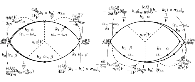
Figure 1: Feynman diagram of a contribution from the side jump to $\sigma_{xy}$ in the normal state. The spin current vertex and charge current vertex come, respectively, $\bm{j}_{{\rm s}x}^{(2)}$ and $\bm{j}_{{\rm c}y}^{(1)}$.

Figure 2: Feynman diagram of a contribution from the side jump to $\sigma_{xy}$ in the normal state. The spin current vertex and charge current vertex, respectively, come from $\bm{j}_{{\rm s},x}^{(1)}$ and $\bm{j}_{{\rm c},y}^{(2)}$.

Figure 3: Feynman diagram of a contribution from the skew scattering to $\sigma_{xy}$ in the normal state.

The quantities assigned to the vertices and the dotted line are inscribed in the Figures. The solid line in the Figures corresponds to the free electron propagator

$$\mathcal{G}_{\alpha}(\bm{k},i\varepsilon_{n})=\frac{1}{i\varepsilon_{n}-\varepsilon_{\bm{k}}+\mu+\frac{i\hbar}{2\tau}\operatorname{sign}(\varepsilon_{n})}.$$ (21)

Here $\varepsilon_{n}=2\pi T(n+1/2)$ is the fermionic Matsubara frequency, $\varepsilon_{\bm{k}}=\hbar^{2}k^{2}/(2m)$ and $\mu$, respectively, the kinetic energy and chemical potential of free electron. The mean free time $\tau$ is given by

$$\tau=\frac{\hbar}{2\pi N(0)n_{\rm i}v_{0}^{2}},$$ (22)

with the density of states $N(0)$ per spin at the Fermi surface in the normal state. The dotted lines represent the random average of the impurity potentials, and the cross marks represent spin-orbit interactions.

Following the standard procedures, we can obtain spin Hall conductivity in the normal state

$$\sigma_{xy}^{\mathrm{SJ(normal)}}= \frac{e^{2}\hbar}{2Dm}\lambda_{0}^{2}k_{\mathrm{F}}^{2}N(0)$$ (23)

$$\sigma_{xy}^{\mathrm{SS(normal)}}= \frac{\pi e^{2}\hbar^{2}}{2D^{2}m^{2}}\lambda_{0}^{2}v_{0}k_{\mathrm{F}}^{4}N(0)^{2}\tau,$$ (24)

with $D=2,3$.

II.2 Intrinsic spin Hall effect

We summarize the earlier results on intrinsic spin Hall effect developed by Sinova et al. [11] for the two-dimensional electron gas with Rashba spin-orbit interactions.

II.2.1 Hamitonian, Spin current density, and Charge current density

The Hamiltonian of the two-dimensional electron gas (2DEG) with Rashba-type spin-orbit interaction is written as

$$H= \frac{\bm{p}^{2}}{2m}I-\frac{\lambda}{\hbar}\bm{\sigma}\dotproduct(\hat{\bm{z}}\crossproduct\bm{p})$$ (25)

$$= \matrixquantity(\frac{\bm{p}^{2}}{2m}&\frac{\lambda}{\hbar}(p_{y}+ip_{x})\\ \frac{\lambda}{\hbar}(p_{y}-ip_{x})&\frac{\bm{p}^{2}}{2m}),$$ (26)

where the region of 2DEG is taken to be $xy$ plane, which is perpendicular to the unit vector $\hat{\bm{z}}$ parallel to $z$-axis. $I$, $\bm{\sigma}={}^{t}(\sigma^{x},\sigma^{y},\sigma^{z})$ are, respectively, the 2 by 2 unit matrix and the Pauli matrices in the spin space. The symbol $\lambda$ represents the coupling parameter of spin-orbit interaction, which is different from $\lambda_{0}$ used in extrinsic Hall effect. The eigenvalues of this Hamiltonian $H$ are given by

$$\varepsilon_{\pm}(\bm{p})=\frac{p^{2}}{2m}\pm\frac{\lambda}{\hbar}p.$$ (27)

The eigenvectors are given by

$$\ket{\chi_{\pm}(\bm{p})}\equiv\frac{1}{\sqrt{2}}\matrixquantity(\pm\frac{1}{p}(p_{y}+ip_{x})\\ 1)$$ (28)

in spin space. Let $\psi_{\bm{k}\sigma}$ be the Fourier transform of the field operator $\psi_{\sigma}(\bm{r})$ for annihilation of particle at the position $\bm{r}$ with $z$-component of spin $\sigma$. This operator $\psi_{\bm{k}\sigma}$ is expanded in terms of the annihilation operator $c_{\bm{p}\alpha}$ of the eigenstate of the Hamiltonian with spin state $\ket{\chi_{\alpha}(\bm{p})}$ for $\alpha=\pm$ as

$$\psi_{\bm{k}\sigma}= \sum_{\alpha=\pm}\frac{1}{\sqrt{2}}\quantity[\alpha\delta_{\sigma\uparrow}\frac{1}{k}(k_{y}+ik_{x})+\delta_{\sigma\downarrow}]c_{\bm{k}\alpha}.$$ (29)

We define the spin current density as $\bm{J}_{\mathrm{s}}=-(e/4)\anticommutator{\sigma^{z}}{\bm{u}}$ in the same way as (7) but differently from Sinova et al.(2004) [11]. The velocity operator $\bm{u}$ is given by

$$\bm{u}=\frac{i}{\hbar}\commutator{H}{\bm{r}}=\frac{\bm{p}}{m}-\frac{\lambda}{\hbar}\bm{\sigma}\crossproduct\hat{\bm{z}},$$ (30)

which is followed by

$$\bm{J}_{\mathrm{s}}=-e\frac{\bm{p}}{2m}\sigma^{z}.$$ (31)

The uniform component of the Fourier transform of Eq. (31) is given by

$$\bm{j}_{\mathrm{s}}= -e\sum_{\sigma\bm{k}}\frac{\hbar\bm{k}}{2m}\sigma_{\sigma\sigma}^{z}\psi_{\bm{k}\sigma}^{\dagger}\psi_{\bm{k}\sigma},$$ (32)

which is rewritten as

$$\bm{j}_{\mathrm{s}}=e\sum_{\bm{k}\alpha}\frac{\hbar\bm{k}}{2m}c_{\bm{k}\alpha}^{\dagger}c_{\bm{k}-\alpha}.$$ (33)

The charge current density $\bm{j}_{\mathrm{c}}$ is given by the sum of the free electron part due to the kinetic energy and that due to the spin-orbit interaction $H_{\mathrm{SO}}$. We focus on the latter, which we denote by $\bm{j}_{\mathrm{c}}^{\rm SO}(\bm{r})$. The spin orbit interaction $H_{\mathrm{SO}}$ is written in the form of the second quantization

$$H_{\mathrm{SO}}= -\frac{\lambda}{\hbar}\sum_{\sigma\sigma^{\prime}}\int d\bm{r}\;\psi_{\sigma}^{\dagger}(\bm{r})\bm{\sigma}_{\sigma\sigma^{\prime}}\dotproduct\quantity(\hat{\bm{z}}\crossproduct\frac{\hbar}{i}\gradient)\psi_{\sigma^{\prime}}(\bm{r}).$$ (34)

From the relation $\divergence\bm{j}_{\mathrm{c}}^{\rm SO}(\bm{r})=-(ie/\hbar)\commutator{\sum_{\sigma}\psi^{\dagger}_{\sigma}(\bm{r})\psi_{\sigma}(\bm{r})}{H_{\mathrm{SO}}}$ and

$$-\frac{ie}{\hbar}\commutator{\sum_{\sigma}\psi^{\dagger}_{\sigma}(\bm{r})\psi_{\sigma}(\bm{r})}{H_{\mathrm{SO}}}=\divergence\quantity[\frac{e\lambda}{\hbar}\sum_{\sigma\sigma^{\prime}}\quantity(\bm{\sigma}_{\sigma\sigma^{\prime}}\crossproduct\hat{\bm{z}})\psi_{\sigma}^{\dagger}(\bm{r})\psi_{\sigma^{\prime}}(\bm{r})],$$ (35)

we obtain

$$\bm{j}^{\mathrm{SO}}_{\mathrm{c}}(\bm{r})= \frac{e\lambda}{\hbar}\sum_{\sigma\sigma^{\prime}}(\bm{\sigma}_{\sigma\sigma^{\prime}}\crossproduct\hat{\bm{z}})\psi_{\sigma}^{\dagger}(\bm{r})\psi_{\sigma^{\prime}}(\bm{r}).$$ (36)

The uniform component of the Fourier transform of $\bm{j}^{\mathrm{SO}}_{\mathrm{c}}(\bm{r})$ is given by

$$\bm{j}_{\mathrm{c}}^{\mathrm{SO}}= \frac{e\lambda}{\hbar}\sum_{\sigma\sigma^{\prime}}(\bm{\sigma}_{\sigma\sigma^{\prime}}\crossproduct\hat{\bm{z}})\sum_{\bm{k}}\psi_{\bm{k}\sigma}^{\dagger}\psi_{\bm{k}\sigma^{\prime}}.$$ (37)

By adding the part $\bm{j}_{\mathrm{c}}^{(1)}$ due to kinetic energy, the uniform component of the Fourier transform of $\bm{j}_{\mathrm{c}}(\bm{r})$ is given by

$$\bm{j}_{\mathrm{c}}=-\sum_{\bm{k}\sigma}e\frac{\hbar\bm{k}}{m}\psi_{\bm{k}\sigma}^{\dagger}\psi_{\bm{k}\sigma}+\frac{e\lambda}{\hbar}\sum_{\sigma\sigma^{\prime}}(\bm{\sigma}_{\sigma\sigma^{\prime}}\crossproduct\hat{\bm{z}})\sum_{\bm{k}}\psi_{\bm{k}\sigma}^{\dagger}\psi_{\bm{k}\sigma^{\prime}}.$$

The $y$-component of $\bm{j}_{\mathrm{c}}$ is expressed in terms of creation/annihilation operator of the energy eigenstates as

$$j_{\mathrm{c}y}= \sum_{\bm{k}\alpha}\quantity[-\frac{e\hbar}{m}k_{y}c_{\bm{k}\alpha}^{\dagger}c_{\bm{k}\alpha}+\frac{e\lambda}{\hbar}\quantity(-\frac{k_{y}}{k}\alpha c_{\bm{k}\alpha}^{\dagger}c_{\bm{k}\alpha}+i\frac{k_{x}}{k}\alpha c_{\bm{k}\alpha}^{\dagger}c_{\bm{k}-\alpha})].$$ (38)

II.2.2 Spin Hall conductivity

Figure 4 shows the diagram representing the lowest order process for spin Hall effect.

Figure 4: Feynman diagram for the lowest order process for intrinsic spin Hall effect.

The response function $\Phi_{xy}(\bm{q},i\omega_{\nu})$ and the spin Hall conductivity $\sigma_{xy}(\bm{q},\omega)$ are obtained by using Eq. (19) and Eq. (20) as in the extrinsic case. It then suffices to calculate the response function, which is written as

$$\Phi_{xy}(0,i\omega_{\nu})= -\frac{1}{V}\sum_{\alpha}\sum_{\bm{k}}T\sum_{n}\quantity(\frac{e\hbar}{2m}k_{x})\quantity(i\frac{e\lambda}{\hbar}\frac{k_{x}}{k}\alpha)\mathcal{G}_{\alpha}(\bm{k},i\varepsilon_{n})\mathcal{G}_{-\alpha}(\bm{k},i\varepsilon_{n}-i\omega_{\nu})$$ (39)

$$= -\frac{1}{V}\sum_{\alpha}\alpha\sum_{\bm{k}}\frac{ie^{2}\lambda}{2m}\frac{k_{x}^{2}}{k}\frac{f\bm{(}\varepsilon_{\alpha}(\bm{k})\bm{)}-f\bm{(}\varepsilon_{-\alpha}(\bm{k})\bm{)}}{\varepsilon_{\alpha}(\bm{k})-\varepsilon_{-\alpha}(\bm{k})-i\omega_{\nu}}$$ (40)

in terms of the green function

$$\mathcal{G}_{\alpha}(\bm{k},i\varepsilon_{n})=\frac{1}{i\varepsilon_{n}-\quantity(\frac{\hbar^{2}k^{2}}{2m}+\alpha\lambda k)+\mu}.$$ (41)

With use of Eq. (19), $\sigma_{xy}(0,\omega\to 0)$ becomes [11]

$$\sigma_{xy}(0,\omega\to 0)\approx -\frac{\hbar e^{2}}{16\pi m\lambda}\int_{0}^{\infty}dk\;2\lambda kf^{\prime}\quantity(\frac{\hbar^{2}k^{2}}{2m})=\frac{e^{2}}{8\pi\hbar}f(0)\approx\frac{e^{2}}{8\pi\hbar}$$ (42)

in the case where $\lambda k_{\mathrm{F}}\ll\varepsilon_{\mathrm{F}}$. Note that $\sigma_{xy}(0,\omega\to 0)$ does not depend on $\lambda$.

Exceptional simplicity of this model, viz, combination of parabolic band dispersion and linear momentum dependence of the spin-orbit interaction makes the spin Hall conductivity vanish in the presence of spin-conserving impurities, even in the limit of weak scatterers[39, 40, 41, 42, 43, 44, 16, 45]. However, this model is of importance to address the two-body interaction effect on the spin Hall effect[43, 46]. We will thus adopt the Rashba model with an attractive short-range interaction in sec. IV to consider the superconducting fluctuation contribution to the spin Hall effect. The superconducting property of this model was discussed in [47, [][[Sov.Phys.JETP$\bm{68}$1244(1989)].]Edelstein1989].

II.3 Cooperon and fluctuation propagator

In this subsection, we give an overview of Cooperon and superconducting fluctuations, following the description in reference [36]. We add the BCS-type two-body attractive interaction to the Hamiltonian $H_{0}$ in the normal state Eq. (2)

$$H_{\rm int}=-\frac{g}{V}\sum_{\bm{k}\bm{k}^{\prime}\bm{q}}\psi_{\bm{k}+\bm{q},\uparrow}^{\dagger}\psi_{-\bm{k},\downarrow}^{\dagger}\psi_{-\bm{k}^{\prime},\downarrow}\psi_{\bm{k}^{\prime}+\bm{q},\uparrow}$$ (43)

in order to take account of the three types of the superconducting fluctuation effect. We define the Cooperon and fluctuation propagator of superconductivity in this subsection.

The shaded region represents the Cooperon $C(\bm{q},\varepsilon_{1},\varepsilon_{2})$, which is defined through the recursive relation

$$C(\bm{q},\varepsilon_{1},\varepsilon_{2})= 1+\frac{1}{V^{2}}n_{i}v_{0}^{2}V\sum_{\bm{p}}\mathcal{G}(\bm{p}+\bm{q},i\varepsilon_{1})\mathcal{G}(-\bm{p},i\varepsilon_{2})C(\bm{q},\varepsilon_{1},\varepsilon_{2})$$ (44)

or graphically by Fig. 5. Explicit expression for $C(\bm{q},\varepsilon_{1},\varepsilon_{2})$ is give by

$$C(\bm{q},\varepsilon_{1},\varepsilon_{2})= \frac{\absolutevalue{\widetilde{\varepsilon}_{1}-\widetilde{\varepsilon}_{2}}}{\absolutevalue{\varepsilon_{1}-\varepsilon_{2}}+\frac{\hbar}{\tau}\frac{\expectationvalue{(\hbar\bm{v}_{\mathrm{F}}\dotproduct\bm{q})^{2}}_{\mathrm{F.S.}}}{\absolutevalue{\widetilde{\varepsilon}_{1}-\widetilde{\varepsilon}_{2}}^{2}}\theta(-\varepsilon_{1}\varepsilon_{2})}.$$ (45)

Figure 5: $C(\bm{q},\varepsilon_{1},\varepsilon_{2})$.

From this expression, we see that $C(\bm{q},\varepsilon_{1},\varepsilon_{2})$ becomes small unless

$$\frac{\expectationvalue{(\hbar\bm{v}_{\mathrm{F}}\dotproduct\bm{q})^{2}}_{\mathrm{F.S.}}}{\tau/\hbar\absolutevalue{\widetilde{\varepsilon}_{1}-\widetilde{\varepsilon}_{2}}^{2}}\lesssim\absolutevalue{\varepsilon_{1}-\varepsilon_{2}}$$ (46)

is satisfied. The condition (46) reduces to

$$q\ll \frac{1}{\hbar v_{\mathrm{F}}}\absolutevalue{\widetilde{\varepsilon}_{1}-\widetilde{\varepsilon}_{2}}\sqrt{\frac{T\tau}{\hbar}}\sim\begin{dcases}\frac{T}{\hbar v_{\mathrm{F}}}\sqrt{\frac{T\tau}{\hbar}}&(\text{when }T\tau/\hbar\gg 1)\\ \frac{1}{\tau v_{\mathrm{F}}}\sqrt{\frac{T\tau}{\hbar}}&(\text{when }T\tau/\hbar\ll 1).\end{dcases}$$ (47)

This implies that the integral region with $\bm{q}$ is practically reduced to the region where the condition (47) is satisfied.

The wavy lines represent the propagator of superconducting fluctuation, $L(\bm{q},i\Omega_{k})$, which is defined by Eq. (48) and graphically by Fig. 6.

$$L(\bm{q},i\Omega_{k})=-\frac{g}{V}+\frac{g}{V}T\sum_{n^{\prime\prime},p^{\prime\prime}}\mathcal{G}(\bm{p}^{\prime\prime}+\bm{q},i\varepsilon_{n^{\prime\prime}+k})\mathcal{G}(-\bm{p}^{\prime\prime},-i\varepsilon_{n^{\prime\prime}})C(\bm{q},\varepsilon_{n^{\prime\prime}+k},-\varepsilon_{n^{\prime\prime}})L(\bm{q},i\Omega_{k}).$$ (48)

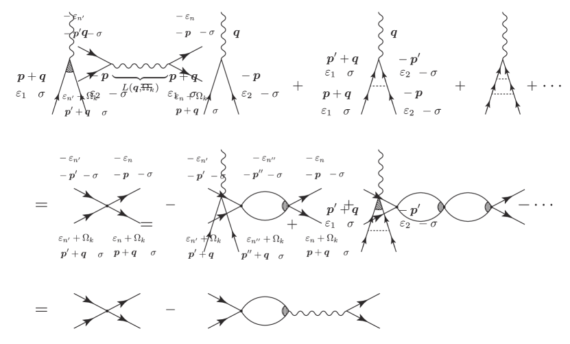
Figure 6: Diagramatical definition of $L(\bm{q},i\Omega_{k})$.

Explicit expression for $L(\bm{q},i\Omega_{k})$ is given by

$$L(\bm{q},i\Omega_{k})=-\frac{1}{VN(0)}\frac{1}{\epsilon+\psi\quantity(\frac{1}{2}+\frac{\absolutevalue{\Omega_{k}}}{4\pi T})-\psi\quantity(\frac{1}{2})+\xi_{\text{\scalebox{0.7}{{\hbox{\mathrm{SC}}}}}}^{2}\bm{q}^{2}}\approx-\frac{1}{VN(0)}\frac{1}{\epsilon+\frac{\pi\absolutevalue{\Omega_{k}}}{8T}+\xi_{\text{\scalebox{0.7}{{\hbox{\mathrm{SC}}}}}}^{2}\bm{q}^{2}},$$ (49)

where we have introduced the coherence length $\xi_{\text{\scalebox{0.7}{$\mathrm{SC}$}}}$ and diffusion constant $\mathcal{D}$

$$\xi_{\text{\scalebox{0.7}{$\mathrm{SC}$}}}^{2}=\frac{\pi\hbar}{8T}\mathcal{D}=-\frac{v_{\mathrm{F}}^{2}\tau^{2}}{D}\quantity[\psi\quantity(\frac{1}{2}+\frac{\hbar}{4\pi T\tau})-\psi\quantity(\frac{1}{2})-\frac{\hbar}{4\pi T\tau}\psi^{(1)}\quantity(\frac{1}{2})].$$ (50)

Here the di-Gamma function $\psi(z)\equiv\derivative{z}\ln\Gamma(z)=\lim_{n_{\mathrm{c}}\to\infty}[-\sum_{n=0}^{n_{\mathrm{c}}-1}\frac{1}{n+z}+\ln n_{\mathrm{c}}]$ and $n$-th order derivative of $\psi(z)$, which we denote by $\psi^{(n)}(z)$ (polyGamma function) are introduced. The coherence length reduces to

$$\xi_{\text{\scalebox{0.7}{$\mathrm{SC}$}}}= \begin{dcases}\sqrt{\frac{7\zeta(3)}{16\pi^{2}D}}\frac{\hbar v_{\mathrm{F}}}{T}&(T\tau/\hbar\gg 1)\\ \sqrt{\frac{\pi}{8D}}v_{\mathrm{F}}\tau\sqrt{\frac{\hbar}{T\tau}}&(T\tau/\hbar\ll 1)\end{dcases}$$ (51)

in the dirty and clean limits, respectively.

III Fluctuation effects on extrinsic spin Hall conductivity

Near and above the superconducting transition temperature $T_{\rm c}$, we take account of the superconducting fluctuation via three types of the process; Aslamazov-Larkin (AL) term, the Maki-Thompson (MT) term, and the density of states (DOS) term. Those are known to be the most diverging in the electric conductivity when $T\rightarrow T_{\rm c}+0$.

III.1 Aslamazov-Larkin terms

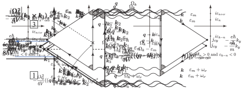
(a)

(b)

(c)

Figure 7: The diagram for the AL term in the presence of side jump.

In this section, we consider the Hamiltonian $H=H_{0}+H_{\mathrm{SO}}+\mathcal{V}+H_{\mathrm{int}}$, which is the sum of Eq. (2) and Eq. (43). The Feynman diagrams [of the charge current-spin current correlation function $\Phi_{xy}^{\mathrm{AL}}(0,i\omega_{\nu})$] for the AL terms with side jump are shown in Fig. 7 and those for AL terms with skew scattering are shown in Fig. 8. We denote $\mathcal{B}_{\mathrm{c}}(\bm{q},\omega,\Omega)$ by the triangular part containing the charge current vertex (i.e. renormalized charge current vertex) and $\mathcal{B}_{\mathrm{s}}(\bm{q},\omega,\Omega)$ by the renormalized spin current vertex, respectively. The response function is then given by

$$\Phi_{xy}(0,i\omega_{\nu})= \frac{1}{V}\sum_{\bm{q}}T\sum_{\Omega_{k}}L(\bm{q},i\Omega_{k})L(\bm{q},i\Omega_{k}+i\omega_{\nu})\mathcal{B}_{\mathrm{s}}(\bm{q},i\Omega_{k},i\omega_{\nu})\mathcal{B}_{\mathrm{c}}(\bm{q},i\Omega_{k},i\omega_{\nu}).$$ (52)

The $O(\omega)$ contributions in Eq. (52) yields the spin Hall conductivity. In the electric conductivity, we can deduce the main contribution in the AL term by setting $\omega=0$ and $\Omega=0$ in the charge current vertices $\mathcal{B}_{\rm c}(\bm{q},\omega,\Omega)$ and retaining $O(\omega)$ part in the fluctuation propagators. In contrast, in the spin Hall conductivity, the contributions with $\mathcal{B}_{\rm s}(\bm{q},0,0)$ vanishes and thus we have to maintain the frequencies $\Omega,\omega$ to be finite. Accordingly, the procedure to calculate the spin Hall conductivity, which is given below, is slightly different from that for AL term in electric conductivity,

1. List the relevant diagrams (Fig. 7 for AL+ side jump and Fig. 8 for AL + skew scattering) and write down the expressions for the charge current-spin current correlation function $\Phi_{xy}^{\mathrm{AL}}(0,i\omega_{\nu})$.

2. Expand $\mathcal{B}_{\mathrm{c}}(\bm{q},\omega,\Omega)$ and $\mathcal{B}_{\mathrm{s}}(\bm{q},\omega,\Omega)$ with respect of $\bm{q}$ up to the first order as $\mathcal{B}_{\mathrm{s}}(\bm{q},\omega,\Omega)\approx-i\zeta_{\rm s}Vq_{y}B_{\mathrm{s}}(\omega,\Omega)$ and $\mathcal{B}_{\mathrm{c}}(\bm{q},\omega,\Omega)\approx\zeta_{\rm c}q_{y}VB_{\mathrm{c}}(\omega,\Omega)$ with coefficients $\zeta_{\rm s}$ and $\zeta_{\rm c}$.

3. Perform integrals in the expressions for $B_{\mathrm{c}}$ and $B_{\mathrm{s}}$ with respect to internal wave vectors $\bm{k}_{1},\bm{k}_{2}\cdots$.

4. Transform the sum with $\Omega_{k}$ to contour integral.

5. Expand the resultant expression with respect to $\omega$ after analytic continuation $i\omega_{\nu}\to\hbar\omega$.

6. Retain the most singular terms in the limit of $\epsilon\to 0$.

7. Perform summation in $B_{\mathrm{c}}(\bm{q},\omega,\Omega)$, $B_{\mathrm{s}}(\bm{q},\omega,\Omega)$ with respect to internal frequencies $\varepsilon_{n}$ and $\varepsilon_{m}$.

8. Integrate the resultant expression with respect to $\bm{q}$.

The details of calculation along these procedures are given in Supplemental materials. Here we outline the flow of calculations. After Step 3, the response function reduces to

$$\Phi_{xy}(0,i\omega_{\nu})\approx -i\zeta_{\rm s}\zeta_{\rm c}V\sum_{\bm{q}}\frac{\bm{q}^{2}}{D}T\sum_{\Omega_{k}}L(\bm{q},i\Omega_{k})L(\bm{q},i\Omega_{k}+i\omega_{\nu})B_{\mathrm{s}}(i\Omega_{k},i\omega_{\nu})B_{\mathrm{c}}(i\Omega_{k},i\omega_{\nu}).$$ (53)

After Steps 4 and 5, we find that

$$\quantity[T\sum_{\Omega_{k}}L(\bm{q},i\Omega_{k})L(\bm{q},i\Omega_{k}+i\omega_{\nu})B_{\mathrm{c}}(i\Omega_{k},i\omega_{\nu})B_{\mathrm{s}}(i\Omega_{k},i\omega_{\nu})]_{i\omega_{\nu}\to\hbar\omega\approx 0}$$ (54)

$$= \hbar\omega\frac{T}{2}L(\bm{q},0)^{2}B_{\mathrm{c}2}(0,0)\derivative{x}\quantity[B_{\mathrm{s}2}(-x,x)+B_{\mathrm{s}2}(0,x)]_{x=0}+\hbar\omega(\mbox{regular terms in the limit $\epsilon\rightarrow+0$})+O(\omega^{2}).$$ (55)

Here $B_{\mathrm{c,s2}}(Z,z)$ is analytic continuation $(i\Omega_{k}\rightarrow Z,i\omega_{\nu}\rightarrow z)$ of $B_{\mathrm{c,s}}(i\Omega_{k},i\omega_{\nu})$ under the condition $-{\rm Im}z<{\rm Im}Z<0$.

After Step 7, we obtain the expressions for $\derivative{x}\quantity[B_{\mathrm{s}2}(-x,x)+B_{\mathrm{s}2}(0,x)]_{x=0}$ and $B_{\mathrm{c}2}(0,0)$ in terms of $\hbar/\tau$ and $T$. After Step 8, we obtain

$$V\sum_{\bm{q}}\bm{q}^{2}L(\bm{q},0)^{2}\approx \frac{1}{4\pi N(0)^{2}\xi_{\text{\scalebox{0.7}{$\mathrm{SC}$}}}^{4}}\ln\frac{1}{\epsilon}$$ (56)

for $D=2$ and

$$V\sum_{\bm{q}}\bm{q}^{2}L(\bm{q},0)^{2}\approx \frac{1}{2\pi^{2}N(0)^{2}\xi_{\text{\scalebox{0.7}{$\mathrm{SC}$}}}^{5}}$$ (57)

for $D=3$.

Finally, the resultant expression for the AL term of the spin Hall conductivity in the side jump process is given by

$$\sigma_{xy}^{\mathrm{AL-SJ}}\approx \frac{2e^{2}\hbar}{Dm}\lambda_{0}^{2}k_{\mathrm{F}}^{2}\frac{T}{\varepsilon_{\mathrm{F}}}N(0)\begin{dcases}\frac{1}{2}\ln\frac{1}{\epsilon}&(D=2)\\ \frac{1}{\pi\xi_{\text{\scalebox{0.7}{$\mathrm{SC}$}}}}&(D=3).\end{dcases}$$ (58)

For $D=2$, the ratio of fluctuation conductivity to that in the normal state is given by

$$\sigma_{xy}^{\mathrm{AL-SJ}}/\sigma_{xy}^{\mathrm{SJ(normal)}}= 2\frac{T}{\varepsilon_{\mathrm{F}}}\ln\frac{1}{\epsilon}$$ (59)

with use of Eq. (23).

The expression for the AL term of the spin Hall conductivity in the skew scattering process is given by

$$\sigma_{xy}^{\mathrm{AL-SS}}= \frac{8\pi^{2}e^{2}\hbar^{7}\lambda_{0}^{2}n_{\mathrm{i}}v_{0}^{3}k_{\mathrm{F}}^{6}N(0)^{2}T}{D^{4}m^{4}}\quantity(\frac{\tau}{\hbar})^{6}$$

$$\times\quantity[\frac{\hbar}{4\pi T\tau}\psi^{(1)}\quantity(\frac{1}{2})+\psi\quantity(\frac{1}{2})-\psi\quantity(\frac{1}{2}+\frac{\hbar}{4\pi T\tau})]$$

$$\times\quantity[2\frac{\hbar}{4\pi T\tau}\psi^{(1)}\quantity(\frac{1}{2})+\frac{\hbar}{4\pi T\tau}\psi^{(1)}\quantity(\frac{1}{2}+\frac{\hbar}{4\pi T\tau})+3\psi\quantity(\frac{1}{2})-3\psi\quantity(\frac{1}{2}+\frac{\hbar}{4\pi T\tau})]$$

$$\times\begin{dcases}\frac{1}{4\pi\xi_{\text{\scalebox{0.7}{$\mathrm{SC}$}}}^{4}}\ln\frac{1}{\epsilon}&(D=2)\\ \frac{1}{2\pi^{2}\xi_{\text{\scalebox{0.7}{$\mathrm{SC}$}}}^{5}}&(D=3).\end{dcases}$$ (60)

In the dirty limit$(T\tau\ll 1)$ in $D=2$ systems, Eq. (60) reduces to

$$\sigma_{xy}^{\mathrm{AL-SS}}/\sigma_{xy}^{\mathrm{SS(normal)}}= 4\frac{T}{\varepsilon_{\mathrm{F}}}\ln\frac{1}{\epsilon}$$ (61)

with use of Eqs. (22), (24), (50). In the clean limit ($T\tau/\hbar\gg 1$) in the two dimensional systems $D=2$, Eq. (60) reduces to

$$\sigma_{xy}^{\mathrm{AL-SS}}/\sigma_{xy}^{\mathrm{SS(normal)}}=2\frac{T}{\varepsilon_{\mathrm{F}}}\ln\frac{1}{\epsilon}.$$

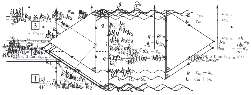
(a)

(b)

(c)

(d)

Figure 8: The diagram for the AL term in the presence of skew scattering.

III.2 DOS terms

The DOS terms for the spin Hall conductivity are calculated in a way similar to those for electric conductivity. The procedure to calculate the spin Hall conductivity is given below.

1. List the relevant diagrams (Fig. 9 for DOS + side jump, and Fig. 10 for DOS + skew scattering) and write down the expressions for the charge current-spin current correlation function $\Phi_{xy}^{\mathrm{DOS}}(0,i\omega_{\nu})$.

2. Put $\Omega_{k}=0$ in all quantities and $\bm{q}=0$ in all but $L(\bm{q},i\Omega_{k})$.

3. Perform integration with respect to internal wave vectors $\bm{k}_{1},\bm{k}_{2}\cdots$ with use of residue theorem.

4. Reduce the sum with $\varepsilon_{n}$ in the polygamma functions.

5. Expand the resultant expression with respect to $\omega$ after analytic continuation $i\omega_{\nu}\to\hbar\omega$.

6. Perform integration in $L(\bm{q},0)$ with respect to $\bm{q}$.

(a)	(b)
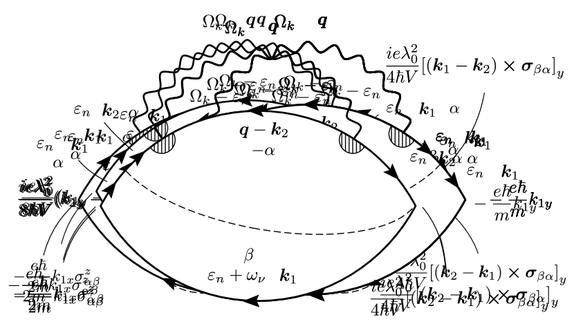
(c)	(d)

Figure 9: Diagrams for DOS term in the presence of side jump process.

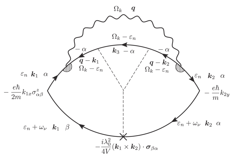
(a)

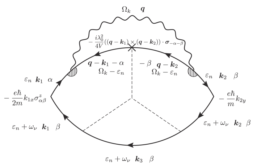
(b)

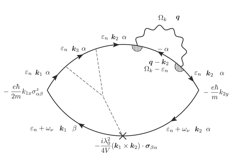
(c)

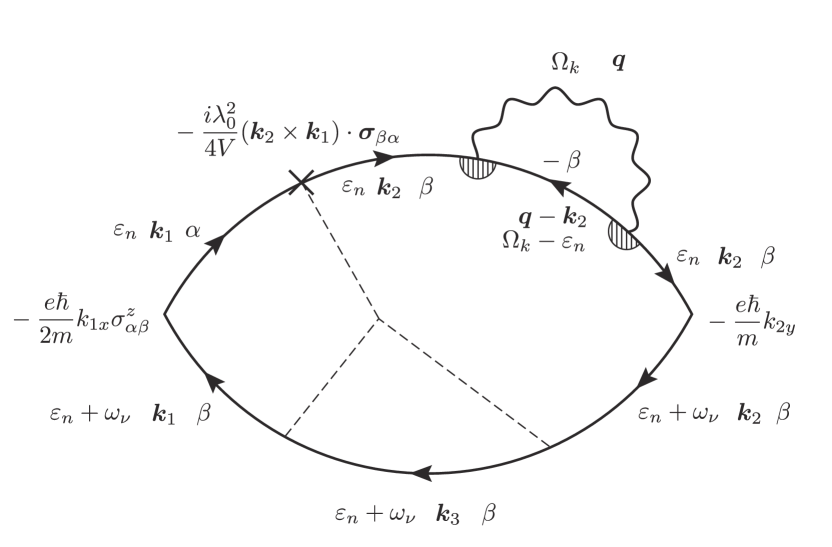
(d)

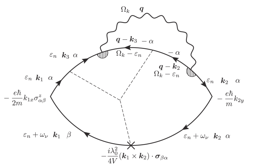
(e)

(f)

Figure 10: Diagrams of DOS terms in the presence of skew scattering.

The details of calculations are given in Supplemental material. However, we here briefly outline the analysis. Figure 9 shows the diagrams of the DOS terms with the side jump process. The diagrams reflected vertically and horizontally give the same contributions as those shown here. The contributions from these diagrams to the spin Hall conductivity are put together as

$$\sigma_{xy}^{\mathrm{DOS-SJ}}= \lim_{\omega\to 0}\frac{e^{2}\lambda_{0}^{2}n_{i}v_{0}^{2}k_{\mathrm{F}}^{2}N(0)^{2}}{mD\omega}T\sum_{\Omega_{k}}\sum_{\bm{q}}L(\bm{q},i\Omega_{k})\Sigma_{xy}^{\mathrm{DOS-SJ}}(\bm{q},i\Omega_{k},\hbar\omega)$$ (62)

$$\Sigma_{xy}^{\mathrm{DOS-SJ}}(\bm{q},i\Omega_{k},i\omega_{\nu})= T\sum_{\varepsilon_{n}}C(\bm{q},\varepsilon_{n},\Omega_{k}-\varepsilon_{n})^{2}(-I^{\rm a}+I^{\rm b}+I^{\rm c}+I^{\rm d}).$$ (63)

Here we introduce the notations $I^{j}(\bm{q},\varepsilon_{n},\Omega_{k},\omega_{\nu})$ with $j={\rm a,b,c,d}$, which we define as the integration of the product of the Green functions obtained in the diagram $j$, where $\xi_{i}\equiv\frac{\hbar^{2}\bm{k}_{i}^{2}}{2m}-\mu$. For example, the expression for $I^{\rm a}(\bm{q},\varepsilon_{n},\Omega_{k},\omega_{\nu})$ is given by

$$I^{a}(\bm{q},\varepsilon_{n},\Omega_{k},\omega_{\nu})=\int d\xi_{1}\;\mathcal{G}(\bm{k}_{1},i\varepsilon_{n})^{2}\mathcal{G}(\bm{k}_{1},i\varepsilon_{n}+i\omega_{\nu})\mathcal{G}(\bm{q}-\bm{k}_{1},i\Omega_{k}-i\varepsilon_{n})\int d\xi_{2}\;\mathcal{G}(\bm{k}_{2},i\varepsilon_{n}+i\omega_{\nu}).$$ (64)

We retain the term with $\Omega_{k}=0$, which yields the most diverging contribution with respect to $\epsilon$. We further retain $\bm{q}$-dependence only in $L(\bm{q},0)$. With these simplification, Eq. (62) becomes

$$\sigma_{xy}^{\mathrm{DOS-SJ}}\approx \lim_{\omega\to 0}\frac{e^{2}\lambda_{0}^{2}n_{i}v_{0}^{2}k_{\mathrm{F}}^{2}N(0)^{2}T}{mD\omega}\Sigma_{xy}^{\mathrm{DOS-SJ}}(0,0,\hbar\omega)\left(\sum_{\bm{q}}L(\bm{q},0)\right).$$ (65)

The part $\Sigma_{xy}^{\mathrm{DOS-SJ}}(0,0,\hbar\omega)$ yields $\omega$-linear term

$$\Sigma^{\mathrm{DOS-SJ}}_{xy}(0,0,\omega)= \hbar\omega\cdot 2\pi\quantity(\frac{\tau}{\hbar})^{3}\quantity[2\psi\quantity(\frac{1}{2})-2\psi\quantity(\frac{1}{2}+\frac{\hbar}{4\pi T\tau})+3\frac{\hbar}{4\pi T\tau}\psi^{(1)}\quantity(\frac{1}{2})-\quantity(\frac{\hbar}{4\pi T\tau})^{2}\psi^{(2)}\quantity(\frac{1}{2})]+O(\omega^{2}),$$ (66)

while the part $\left(\sum_{\bm{q}}L(\bm{q},0)\right)$ in Eq. (65) contributes to singularity in the limit $\epsilon\rightarrow+0$, i. e .,

$$\sum_{\bm{q}}L(\bm{q},0)\approx -\frac{1}{N(0)\xi_{\text{\scalebox{0.7}{$\mathrm{SC}$}}}^{D}}\begin{dcases}\frac{1}{4\pi}\ln\frac{1}{\epsilon}&(D=2)\\ \frac{1}{2\pi^{2}}&(D=3).\end{dcases}$$ (67)

Putting the above results, we arrive at the expression for the DOS terms for extrinsic spin Hall conductivity with the side jump process,

$$\sigma_{xy}^{\mathrm{DOS-SJ}}= -\frac{2\pi e^{2}\lambda_{0}^{2}n_{\mathrm{i}}v_{0}^{2}k_{F}^{2}N(0)T\hbar}{Dm\xi_{\text{\scalebox{0.7}{$\mathrm{SC}$}}}^{D}}\quantity(\frac{\tau}{\hbar})^{3}$$ (68)

$$\times\quantity[2\psi\quantity(\frac{1}{2})-2\psi\quantity(\frac{1}{2}+\frac{\hbar}{4\pi T\tau})+3\frac{\hbar}{4\pi T\tau}\psi^{(1)}\quantity(\frac{1}{2})-\quantity(\frac{\hbar}{4\pi T\tau})^{2}\psi^{(2)}\quantity(\frac{1}{2})]$$ (69)

$$\times\begin{dcases}\frac{1}{4\pi}\ln\frac{1}{\epsilon}&(D=2)\\ \frac{1}{2\pi^{2}}&(D=3).\end{dcases}$$ (70)

For $D=2$, the ratio of the spin Hall conductivity to that in the normal state is

$$\sigma_{xy}^{\mathrm{DOS-SJ}}/\sigma_{xy}^{\mathrm{SJ(normal)}}= -\frac{7\zeta(3)}{\pi^{3}}\frac{\hbar/\tau}{\varepsilon_{\mathrm{F}}}\ln\frac{1}{\epsilon}$$ (71)

in the dirty limit and

$$\sigma_{xy}^{\mathrm{DOS-SJ}}/\sigma_{xy}^{\mathrm{SJ(normal)}}=-\frac{2\pi^{3}}{7\zeta(3)}\frac{T}{\varepsilon_{\mathrm{F}}}\frac{T\tau}{\hbar}\ln\frac{1}{\epsilon}$$ (72)

in the clean limit. The opposite sign between the DOS terms and the spin Hall conductivity in the normal state is consistent with the suppression of the density of state by the superconducting fluctuation.

The expression for the DOS term of the spin Hall conductivity in the skew scattering process is given by

$$\sigma^{\mathrm{DOS-SS}}_{xy}= -\frac{e^{2}\hbar^{3}\lambda_{0}^{2}n_{\mathrm{i}}v_{0}^{3}N(0)^{2}T}{2m^{2}\xi_{\text{\scalebox{0.7}{$\mathrm{SC}$}}}^{D}}\quantity(\frac{k_{\mathrm{F}}^{2}}{D})^{2}$$ (73)

$$\times 8\pi^{2}\quantity(\frac{\tau}{\hbar})^{4}\Biggl{\{}\begin{aligned} -&3\quantity[\psi\quantity(\frac{1}{2}+\frac{\hbar}{4\pi T\tau})-\psi\quantity(\frac{1}{2})]+\frac{\hbar}{4\pi T\tau}\quantity[\psi^{(1)}\quantity(\frac{1}{2}+\frac{\hbar}{4\pi T\tau})+3\psi^{(1)}\quantity(\frac{1}{2})]\\ -&\quantity(\frac{\hbar}{4\pi T\tau})^{2}\psi^{(2)}\quantity(\frac{1}{2})\Biggr{\}}\end{aligned}$$ (74)

$$\times\begin{dcases}\frac{1}{4\pi}\ln\frac{1}{\epsilon}&(D=2)\\ \frac{1}{2\pi^{2}}&(D=3).\end{dcases}$$ (75)

For $D=2$, the ratio of the spin Hall conductivity to that in the normal state is

$$\sigma^{\mathrm{DOS-SS}}_{xy}/\sigma_{xy}^{\mathrm{SS(normal)}}= -\frac{14\zeta(3)}{\pi^{3}}\frac{\hbar/\tau}{\varepsilon_{\mathrm{F}}}\ln\frac{1}{\epsilon}.$$ (76)

in the dirty limit and

$$\sigma_{xy}^{\mathrm{DOS-SS}}/\sigma_{xy}^{\mathrm{SJ(normal)}}= -\frac{4\pi^{3}}{7\zeta(3)}\frac{T}{\varepsilon_{\mathrm{F}}}\frac{T\tau}{\hbar}\ln\frac{1}{\epsilon}$$ (77)

in the clean limit. We notice again the opposite sign between the DOS terms and the spin Hall conductivity in the normal state.

III.3 Maki-Thompson terms

The MT terms are calculated similarly to those for DOS terms. The procedure to calculate the MT terms is given below. We note that the MT terms with the side jump process turn out to vanish in a way similar to that for the MT terms in the extrinsic anomalous Hall effect[38].

1. List the relevant diagrams (Fig. 11 for MT + side jump and Fig. 12 for MT + skew scattering) and write down the expressions for the charge current-spin current correlation function $\Phi_{xy}^{\mathrm{MT}}(0,i\omega_{\nu})$.

2. Put $i\Omega_{k}=0$ in all quantities.

3. Perform integration with respect to internal wave vectors $\bm{k}_{1},\bm{k}_{2}\cdots$ with use of the residue theorem.

4. Perform summation over $\varepsilon_{n}$.

5. Expand the resultant expression with respect to $\omega$ after analytic continuation $i\omega_{\nu}\to\hbar\omega$.

6. Separate regular part and anomalous part. All factors in the former is regular but $L(\bm{q},0)$ is regular in the limit of $\bm{q}\to 0$ while the anomalous part contains singular factor in addition to $L(\bm{q},0)$.

7. Integrate the regular part with $\bm{q}$ after setting $\bm{q}\to 0$ in all quantities but $L(\bm{q},0)$.

8. Integrate the anomalous part with $\bm{q}$ after introducing a phase-breaking relaxation time $\tau_{\varphi}$ to cutoff IR divergence.

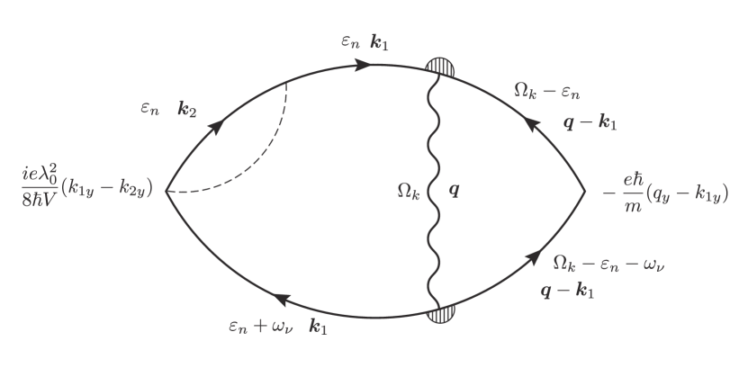
(a)

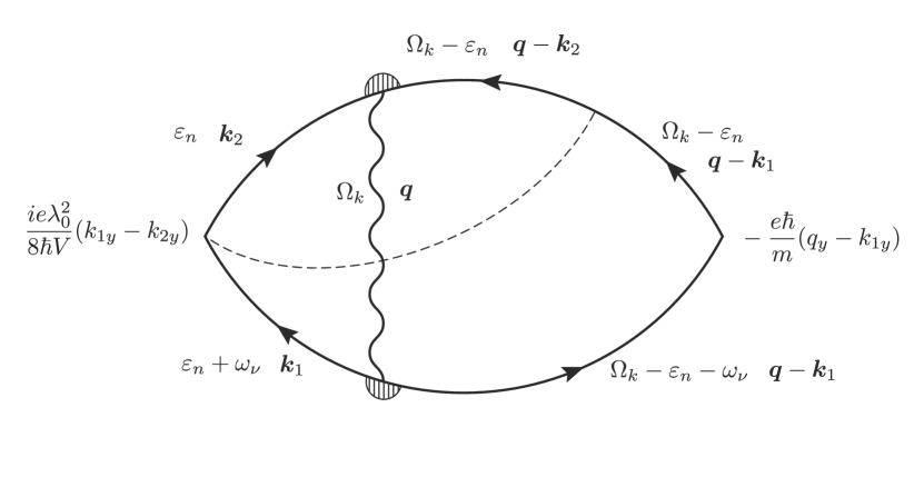
(b)

Figure 11: Diagrams of MT terms in the presence of side jump.

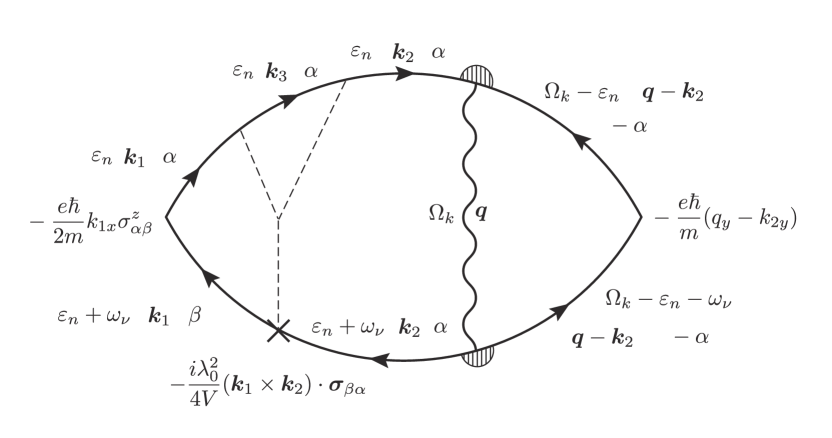
(a)

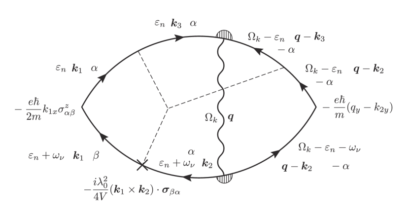
(b)

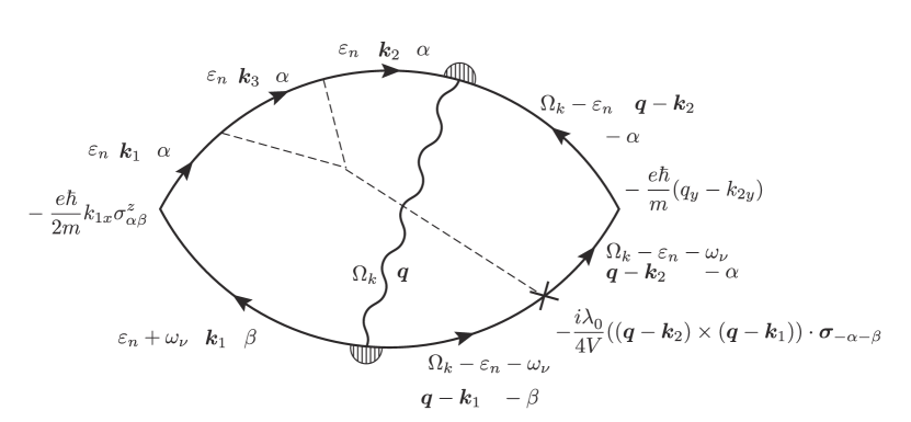
(c)

Figure 12: Diagrams of MT terms in the presence of skew scattering.

The details of the calculation is available in the supplemental material. The diagrams of the MT terms with skew scattering are shown in Fig. 12. The spin Hall conductivity is given in the form of

$$\sigma_{xy}^{\mathrm{MT-SS}}= \lim_{\omega\to 0}\quantity(-\frac{e^{2}\hbar^{2}\lambda_{0}^{2}n_{i}v_{0}^{3}k_{\mathrm{F}}^{4}N(0)^{3}}{D^{2}m^{2}\omega})T\sum_{\Omega_{k}}\sum_{\bm{q}}L(\bm{q},i\Omega_{k})\Sigma_{xy}^{\mathrm{MT-SS}}(\bm{q},i\Omega_{k},\hbar\omega)$$ (78)

$$\Sigma_{xy}^{\mathrm{MT-SS}}(\bm{q},i\Omega_{k},i\omega_{\nu})= T\sum_{\varepsilon_{n}}C(\bm{q},\varepsilon_{n},\Omega_{k}-\varepsilon_{n})C(\bm{q},\varepsilon_{n}+\omega_{\nu},\Omega_{k}-\varepsilon_{n}-\omega_{\nu})\times\quantity(\begin{minipage}{108.405pt}the sum of the integral of product of Green functions\end{minipage}).$$ (79)

The calculation is similar to that in the DOS terms but we have to separate $\Sigma_{xy}^{\mathrm{MT-SS}}$in the regular part and anomalous part

$$\Sigma_{xy}^{\mathrm{MT-SS}}(\bm{q},0,\omega_{\nu})\xrightarrow{i\omega_{\nu}\to\hbar\omega} \Sigma_{xy}^{\mathrm{MT-SS(reg)}}+\Sigma_{xy}^{\mathrm{MT-SS(an)}}(\bm{q},0,\omega),$$ (81)

$$\Sigma_{xy}^{\mathrm{MT-SS(reg)}}= -\hbar\omega\frac{\tau^{2}}{8T^{2}\hbar^{2}}\psi^{(2)}\quantity(\frac{1}{2}),$$ (82)

$$\Sigma_{xy}^{\mathrm{MT-SS(an)}}(\bm{q},0,\omega)= -\hbar\omega\frac{\pi^{3}\tau^{2}}{4T\hbar^{2}}\frac{1}{-i\hbar\omega+\hbar\mathcal{D}\bm{q}^{2}},$$ (83)

as for the MT terms in the electric conductivity.

As for the regular part, we can proceed in a way similar to that in the DOS terms and obtain

$$\sigma_{xy}^{\mathrm{MT-SS(reg)}}= -\frac{e^{2}\hbar^{3}\lambda_{0}^{2}n_{\mathrm{i}}v_{0}^{3}k_{\mathrm{F}}^{4}N(0)^{2}\tau^{2}}{8D^{2}m^{2}T\hbar^{2}\xi_{\text{\scalebox{0.7}{$\mathrm{SC}$}}}^{D}}\psi^{(2)}\quantity(\frac{1}{2})\begin{dcases}\frac{1}{4\pi}\ln\frac{1}{\epsilon}&(D=2)\\ \frac{1}{2\pi^{2}}&(D=3).\end{dcases}$$ (84)

As for the anomalous part, on the other hand, we introduce the phase breaking time $\tau_{\varphi}$ to cut-off the IR divergence as in the case of electric conductivity[35]. We then obtain

$$\sigma_{xy}^{\mathrm{MT-SS(an)}}= -\frac{\pi^{4}e^{2}\hbar^{3}\lambda_{0}^{2}n_{\mathrm{i}}v_{0}^{3}k_{\mathrm{F}}^{4}N(0)^{2}\tau^{2}}{32D^{2}m^{2}T\hbar^{2}\xi_{\text{\scalebox{0.7}{$\mathrm{SC}$}}}^{D}}\begin{dcases}\frac{1}{4\pi(\epsilon-\gamma_{\varphi})}\ln\frac{\epsilon}{\gamma_{\varphi}}&(D=2)\\ \frac{1}{4\pi(\sqrt{\epsilon}+\sqrt{\gamma_{\varphi}})}&(D=3),\end{dcases}$$ (85)

with the dimensionless cutoff $\gamma_{\varphi}=\pi/8T\tau_{\varphi}$. For $D=2$, the ratio of the spin Hall conductivity to that in the normal state is

$$\sigma^{\mathrm{MT-SS(reg)}}_{xy}/\sigma_{xy}^{\mathrm{SS(normal)}}= \frac{7\zeta(3)}{\pi^{3}}\frac{\hbar/\tau}{\varepsilon_{\mathrm{F}}}\ln\frac{1}{\epsilon},$$ (86)

$$\sigma^{\mathrm{MT-SS(an)}}_{xy}/\sigma_{xy}^{\mathrm{SS(normal)}}= -\frac{\pi}{8}\frac{\hbar/\tau}{\varepsilon_{\mathrm{F}}}\frac{1}{\epsilon-\gamma_{\varphi}}\ln\frac{\epsilon}{\gamma_{\varphi}}$$ (87)

in the dirty limit and

$$\sigma_{xy}^{\mathrm{MT-SS(reg)}}/\sigma_{xy}^{\mathrm{SS(normal)}}= 2\frac{T}{\varepsilon_{\mathrm{F}}}\ln\frac{1}{\epsilon},$$ (88)

$$\sigma_{xy}^{\mathrm{MT-SS(an)}}/\sigma_{xy}^{\mathrm{SS(normal)}}= -\frac{\pi^{4}}{28\zeta(3)}\frac{T}{\varepsilon_{\mathrm{F}}}\frac{1}{\epsilon-\gamma_{\varphi}}\ln\frac{\epsilon}{\gamma_{\varphi}}$$ (89)

in the clean limit.

IV Fluctuation effects on intrinsic spin Hall conductivity in two-dimensional systems with Rashba-type spin-orbit interaction

IV.1 Fluctuation propagator

We first rewrite the two-body interaction with use of Eq. (29) as

$$H_{\mathrm{int}}= -\frac{g}{V}\sum_{\bm{p}\bm{p}^{\prime}\bm{q}}\psi_{\bm{p}+\bm{q},\sigma}^{\dagger}\psi_{-\bm{p},-\sigma}^{\dagger}\psi_{-\bm{p}^{\prime},-\sigma}\psi_{\bm{p}^{\prime}+\bm{q},\sigma}$$ (90)

$$= -\frac{g}{4V}\sum_{\bm{p}\bm{p}^{\prime}\bm{q}}\sum_{\alpha_{1}\sim\alpha_{4}}\alpha_{2}\alpha_{3}\frac{(-p_{y}+ip_{x})(-p^{\prime}_{y}-ip^{\prime}_{x})}{pp^{\prime}}c_{\bm{p}+\bm{q},\alpha_{1}}^{\dagger}c_{-\bm{p},\alpha_{2}}^{\dagger}c_{-\bm{p}^{\prime},\alpha_{3}}c_{\bm{p}^{\prime}+\bm{q},\alpha_{4}}.$$ (91)

Figure 13 shows the diagram of fluctuation propagator.

Figure 13: Feynman diagram for fluctuation propagator.

As an inspection, we examine the diagram containing two $H_{\mathrm{int}}$ (the second term on the right hand side in Fig. 13), which yields

$$T\sum_{\alpha_{5}\alpha_{6}}\sum_{\varepsilon_{n^{\prime\prime}}\bm{p}^{\prime\prime}}\begin{aligned} &\quantity(-\frac{g}{4V})\alpha_{2}\alpha_{6}\frac{(-p^{\prime\prime}_{y}+ip^{\prime\prime}_{x})(-p^{\prime}_{y}-ip^{\prime}_{x})}{p^{\prime\prime}p^{\prime}}\mathcal{G}_{\alpha_{5}}(\bm{p}^{\prime\prime}+\bm{q},i\varepsilon_{n^{\prime\prime}}+i\Omega_{k})\mathcal{G}_{\alpha_{6}}(-\bm{p}^{\prime\prime},-i\varepsilon_{n^{\prime\prime}})\\ \times&\quantity(-\frac{g}{4V})\alpha_{6}\alpha_{3}\frac{(-p_{y}+ip_{x})(-p^{\prime\prime}_{y}-ip^{\prime\prime}_{x})}{pp^{\prime\prime}}\\ \end{aligned}$$ (93)

$$= -\frac{g}{4V}\frac{(-p_{y}+ip_{x})(-p^{\prime}_{y}-ip^{\prime}_{x})}{pp^{\prime}}\alpha_{2}\alpha_{3}T\sum_{\alpha_{5}\alpha_{6}}\sum_{\varepsilon_{n^{\prime\prime}}\bm{p}^{\prime\prime}}\quantity(-\frac{g}{4V})\mathcal{G}_{\alpha_{5}}(\bm{p}^{\prime\prime}+\bm{q},i\varepsilon_{n^{\prime\prime}}+i\Omega_{k})\mathcal{G}_{\alpha_{6}}(-\bm{p}^{\prime\prime},-i\varepsilon_{n^{\prime\prime}}).$$ (94)

This expression does not depend on the internal wave numbers and spins for summation over loops because those dependencies are canceled. Similar cancellation occurs even in the diagrams containing more than two $H_{\mathrm{int}}$, and those diagrams depend only on the left-most and right-most wavenumber and spins. Consequently, the summation over the series of diagrams can be carried out in a way similar to that for superconductors without spin-orbit interaction shown in Fig. 6, i.e.

$$L_{\alpha_{2}\alpha_{3}}(\bm{q},\bm{p},\bm{p}^{\prime},i\Omega_{k})$$ (95)

$$= -\frac{g}{4V}\frac{(-p_{y}+ip_{x})(-p^{\prime}_{y}-ip^{\prime}_{x})}{pp^{\prime}}\alpha_{2}\alpha_{3}$$ (96)

$$\times\begin{aligned} \Biggl{\{}&1-T\sum_{\alpha_{5}\alpha_{6}}\sum_{\varepsilon_{n^{\prime\prime}}\bm{p}^{\prime\prime}}\quantity(-\frac{g}{4V})\mathcal{G}_{\alpha_{5}}(\bm{p}^{\prime\prime}+\bm{q},i\varepsilon_{n^{\prime\prime}}+i\Omega_{k})\mathcal{G}_{\alpha_{6}}(-\bm{p}^{\prime\prime},-i\varepsilon_{n^{\prime\prime}})\\ &+\Biggl{[}T\sum_{\alpha_{5}\alpha_{6}}\sum_{\varepsilon_{n^{\prime\prime}}\bm{p}^{\prime\prime}}\quantity(-\frac{g}{4V})\mathcal{G}_{\alpha_{5}}(\bm{p}^{\prime\prime}+\bm{q},i\varepsilon_{n^{\prime\prime}}+i\Omega_{k})\mathcal{G}_{\alpha_{6}}(-\bm{p}^{\prime\prime},-i\varepsilon_{n^{\prime\prime}})\Biggr{]}^{2}\cdots\Biggr{\}}\end{aligned}$$ (97)

$$= -\frac{1}{4V}\alpha_{2}\alpha_{3}\frac{(-p_{y}+ip_{x})(-p^{\prime}_{y}-ip^{\prime}_{x})}{pp^{\prime}}\quantity[g^{-1}-\Pi(\bm{q},\Omega_{k})]^{-1},$$ (98)

where we introduce the notations

$$\Pi(\bm{q},\Omega_{k})= \frac{1}{4}\sum_{\alpha\beta}T\sum_{\varepsilon_{n}}P_{\alpha\beta}(\bm{q},\varepsilon_{n}+\Omega_{k},-\varepsilon_{n})$$ (99)

$$P_{\alpha\beta}(\bm{q},\varepsilon_{1},\varepsilon_{2})= \frac{1}{V}\sum_{\bm{p}}\mathcal{G}_{\alpha}(\bm{p}+\bm{q},i\varepsilon_{1})\mathcal{G}_{\beta}(-\bm{p},i\varepsilon_{2}).$$ (100)

We find that $P_{\alpha\beta}(\bm{q},\varepsilon_{1},\varepsilon_{2})$ is written as

$$P_{\alpha\beta}(\bm{q},\varepsilon_{1},\varepsilon_{2})= \int\frac{d^{2}\bm{p}}{(2\pi)^{2}}\frac{1}{i\varepsilon_{1}-\quantity(\frac{\hbar^{2}}{2m}(\bm{p}+\bm{q})^{2}+\alpha\lambda\norm{\bm{p}+\bm{q}})+\mu}\frac{1}{i\varepsilon_{2}-\quantity(\frac{\hbar^{2}}{2m}\bm{p}^{2}+\beta\lambda\norm{\bm{p}})+\mu}$$ (101)

$$\approx \int\frac{d^{2}\bm{p}}{(2\pi)^{2}}\frac{1}{i\varepsilon_{1}-\quantity(\frac{\hbar}{2m}p^{2}+\alpha\lambda p-\mu)-\quantity(\frac{\hbar^{2}}{m}+\alpha\frac{\lambda}{p})\bm{p}\dotproduct\bm{q}}\frac{1}{i\varepsilon_{2}-\quantity(\frac{\hbar^{2}}{2m}p^{2}+\beta\lambda p-\mu)},$$ (102)

which becomes when $\lambda p_{\mathrm{F}}\ll\mu$ as

$$P_{\alpha\beta}(\bm{q},\varepsilon_{1},\varepsilon_{2})$$ (103)

$$\approx N(0)\int\frac{d\Omega_{p}}{2\pi}\int d\xi\;\frac{1}{i\varepsilon_{1}-\xi-\alpha\lambda p_{\mathrm{F}}-\quantity(\frac{\hbar^{2}}{m}+\alpha\frac{\lambda}{p_{\mathrm{F}}})\bm{p}_{\mathrm{F}}\dotproduct\bm{q}}\frac{1}{i\varepsilon_{2}-\xi-\beta\lambda p_{\mathrm{F}}}$$ (104)

$$= 2\pi N(0)\theta(-\varepsilon_{1}\varepsilon_{2})\frac{1}{\absolutevalue{\varepsilon_{1}-\varepsilon_{2}}}\quantity{1-\frac{i(\alpha-\beta)\lambda p_{\mathrm{F}}\operatorname{sign}(\varepsilon_{1})}{\absolutevalue{\varepsilon_{1}-\varepsilon_{2}}}-\frac{\quantity[(\alpha-\beta)\lambda p_{\mathrm{F}}]^{2}+\quantity(\frac{\hbar^{2}}{m}+\alpha\frac{\lambda}{p_{\mathrm{F}}})^{2}\expectationvalue{(\bm{p}_{\mathrm{F}}\dotproduct\bm{q})^{2}}_{\mathrm{F.S.}}}{\absolutevalue{\varepsilon_{1}-\varepsilon_{2}}^{2}}}.$$ (105)

We thus see that

$$\frac{1}{4}\sum_{\alpha\beta}P_{\alpha\beta}(\bm{q},\varepsilon_{1},\varepsilon_{2})= 2\pi N(0)\theta(-\varepsilon_{1}\varepsilon_{2})\frac{1}{\absolutevalue{\varepsilon_{1}-\varepsilon_{2}}}\quantity(1-\frac{A(\bm{q})}{\absolutevalue{\varepsilon_{1}-\varepsilon_{2}}^{2}})$$ (106)

with

$$A(\bm{q})= 2(\lambda p_{\mathrm{F}})^{2}+\quantity[\quantity(\frac{\hbar^{2}}{m})^{2}+\quantity(\frac{\lambda}{p_{\mathrm{F}}})^{2}]\expectationvalue{(\bm{p}_{\mathrm{F}}\dotproduct\bm{q})^{2}}_{\mathrm{F.S.}}.$$ (107)

With use of this expression, $\Pi(\bm{q},\Omega_{k})$ becomes

$$\Pi(\bm{q},\Omega_{k})= T\sum_{\varepsilon_{n}}\frac{1}{4}\sum_{\alpha\beta}P_{\alpha\beta}(\bm{q},\varepsilon_{n}+\Omega_{k},-\varepsilon_{n})$$ (108)

$$= N(0)\quantity[\psi\quantity(\frac{1}{2}+\frac{\absolutevalue{\Omega_{k}}}{4\pi T}+\frac{\hbar\omega_{\mathrm{D}}}{2\pi T})-\psi\quantity(\frac{1}{2}+\frac{\absolutevalue{\Omega_{k}}}{4\pi T})+\frac{A(\bm{q})}{2(4\pi T)^{2}}\psi^{(2)}\quantity(\frac{1}{2}+\frac{\absolutevalue{\Omega_{k}}}{4\pi T})].$$ (109)

The transition temperature $T_{\mathrm{c}}$ is determined by the condition that $L(\bm{q}=0,i\Omega_{k}=0)$ diverges at $T\to T_{\mathrm{c}}$, i.e.,

$$0=g^{-1}-\Pi(0,0)= g^{-1}-N(0)\quantity[\psi\quantity(\frac{1}{2}+\frac{\hbar\omega_{\mathrm{D}}}{2\pi T_{\mathrm{c}}})-\psi\quantity(\frac{1}{2})+\frac{A(0)}{2(4\pi T)^{2}}\psi^{(2)}\quantity(\frac{1}{2})].$$ (110)

With use of the relation

$$\epsilon=\ln\frac{T}{T_{\mathrm{c}}}=\ln\quantity(\frac{\hbar\omega_{\mathrm{D}}}{2\pi T_{\mathrm{c}}})-\ln\quantity(\frac{\hbar\omega_{\mathrm{D}}}{2\pi T})\approx\frac{1}{N(0)}\quantity[g^{-1}-\Pi(\bm{q},\Omega_{k})]+\psi\quantity(\frac{1}{2})-\psi\quantity(\frac{1}{2}+\frac{\absolutevalue{\Omega_{k}}}{4\pi T})-\xi_{\text{\scalebox{0.7}{$\mathrm{SC}$}}}^{2}q^{2},$$ (111)

we obtain

$$g^{-1}-\Pi(\bm{q},\Omega_{k})=N(0)\quantity[\epsilon+\psi\quantity(\frac{1}{2}+\frac{\absolutevalue{\Omega_{k}}}{4\pi T})-\psi\quantity(\frac{1}{2})+\xi_{\text{\scalebox{0.7}{{\hbox{\mathrm{SC}}}}}}^{2}q^{2}].$$ (113)

Here we introduce the coherence length in the presence of intrinsic spin-orbit interaction through the relation

$$\xi_{\text{\scalebox{0.7}{$\mathrm{SC}$}}}^{2}q^{2}\equiv -\frac{A(\bm{q})-A(0)}{2(4\pi T)^{2}}\psi^{(2)}\quantity(\frac{1}{2})$$ (114)

$$= -\frac{\quantity(\frac{\hbar^{2}}{m})^{2}+\quantity(\frac{\lambda}{k_{\mathrm{F}}})^{2}}{2(4\pi T)^{2}}\psi^{(2)}\quantity(\frac{1}{2})\expectationvalue{(\bm{k}_{\mathrm{F}}\dotproduct\bm{q})^{2}}_{\mathrm{F.S.}}$$ (115)

$$= -\psi^{(2)}\quantity(\frac{1}{2})\frac{\quantity(\frac{\hbar^{2}}{m})^{2}+\quantity(\frac{\lambda}{k_{\mathrm{F}}})^{2}}{4(4\pi T)^{2}}k_{\mathrm{F}}^{2}q^{2},$$ (116)

which becomes

$$\xi_{\text{\scalebox{0.7}{{\hbox{\mathrm{SC}}}}}}^{2}\approx 14\zeta(3)\frac{\quantity(\frac{\hbar^{2}}{m})^{2}k_{\mathrm{F}}^{2}}{4(4\pi T)^{2}}=\frac{7\zeta(3)}{32\pi^{2}}\frac{\hbar^{2}v_{\mathrm{F}}^{2}}{T^{2}}$$ (117)

because we assume that $\mu\gg\lambda k_{\mathrm{F}}$. With use of Eq. (113) the fluctuation propagator in the presence of spin-orbit interaction is given by

$$L_{\alpha_{1}\alpha_{2}\alpha_{3}\alpha_{4}}(\bm{q},\bm{p},\bm{p}^{\prime},i\Omega_{k})= \quantity(\frac{\alpha_{2}}{2}\frac{-p^{\prime}_{y}-ip^{\prime}_{x}}{p})\quantity(\frac{\alpha_{3}}{2}\frac{-p_{y}+ip_{x}}{p})L(\bm{q},i\Omega_{k})$$ (118)

$$L(\bm{q},i\Omega_{k})\equiv -\frac{1}{N(0)V}\frac{1}{\epsilon+\psi\quantity(\frac{1}{2}+\frac{\absolutevalue{\Omega_{k}}}{4\pi T})-\psi\quantity(\frac{1}{2})+\xi_{\text{\scalebox{0.7}{$\mathrm{SC}$}}}^{2}\bm{q}^{2}}$$ (119)

where $L(\bm{q},i\Omega_{k})$ is the fluctuation propagator without the spin-orbit interaction, which coincides with Eq. (49). In the end of this subsection, we consider $\lambda$ dependence of $T_{\mathrm{c}}$. From Eq. (110), we obtain

$$\frac{T_{\mathrm{c}}}{T_{\mathrm{c}0}}= \exp[-14\zeta(3)\quantity(\frac{\lambda k_{\mathrm{F}}}{4\pi T_{\mathrm{c}}})^{2}],$$ (120)

where $T_{\mathrm{c}0}$ is the transition temperature for $\lambda=0$. From Eq. (120), we find that the transition to superconducting state occurs at a finite temperature when

$$\frac{\lambda k_{\mathrm{F}}}{T_{\mathrm{c}0}}< \frac{2\pi}{\sqrt{7e\zeta(3)}}\approx 1.313\cdots$$ (121)

are satisfied. Figure 14 shows $\lambda$-dependence of $T_{\mathrm{c}}$.

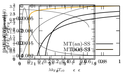
Figure 14: $\lambda$-dependence of $T_{\mathrm{c}}$.

IV.2 Aslamazov-Larkin term

The diagram for AL terms is shown in Fig. 15.

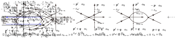
Figure 15: Feynman diagram for the AL term for intrinsic spin Hall effect.

The outline of the procedure to calculate the AL terms for intrinsic spin Hall effect is the same as that for the AL terms for extrinsic spin Hall effect. The details of calculation along these procedures are given in Supplemental materials. The resultant expression for the AL term of the intrinsic spin Hall conductivity is given by

$$\sigma_{xy}^{\mathrm{AL}}\approx \frac{e^{2}\hbar^{5}}{2^{13}\pi^{3}\xi_{\text{\scalebox{0.7}{$\mathrm{SC}$}}}^{4}T\lambda^{2}m^{3}}\quantity[\imaginary\psi^{(1)}\quantity(\frac{1}{2}+\frac{i\lambda k_{\mathrm{F}}}{2\pi T})]^{2}\ln\frac{1}{\epsilon},$$ (122)

which reduces, when $\lambda k_{\mathrm{F}}\ll T$, to

$$\sigma_{xy}^{\mathrm{AL}}\approx \frac{e^{2}}{16\pi\hbar}\frac{T}{\varepsilon_{\mathrm{F}}}\ln\frac{1}{\epsilon}.$$ (123)

IV.3 DOS and Maki-Thompson terms

The DOS term and MT terms in intrinsic spin Hall effects are calculated in a way similar to those in extrinsic spin Hall effect, but there are no anomalous terms in MT terms for intrinsic spin Hall effect, and thus the cutoff is not necessary to be introduced. See the subsections III.2 and III.3, where the procedures to calculate the DOS and MT terms are given. The diagram for the DOS term in intrinsic spin Hall effect is shown in Fig. 16.

Figure 16: Feynman diagram of DOS term in intrinsic spin Hall conductivity.

The DOS term for intrinsic spin Hall conductivity is given by

$$\sigma_{xy}^{\mathrm{DOS}}= -\frac{e^{2}\hbar}{512\pi^{2}m\xi_{\text{\scalebox{0.7}{$\mathrm{SC}$}}}^{2}\lambda k_{\mathrm{F}}}\quantity[-\imaginary\psi^{(1)}\quantity(\frac{1}{2}+\frac{i\lambda k_{\mathrm{F}}}{2\pi T})]\ln\frac{1}{\epsilon}.$$ (124)

Figure 17 shows the profile of $-\imaginary\psi^{(1)}(1/2+ix)$.

Figure 17: Profile of $-\imaginary\psi^{(1)}(1/2+ix)$.

With use of $-\imaginary\psi^{(1)}(1/2+ix)\approx 14\zeta(3)x$ for $x\ll 1$, we obtain

$$\sigma_{xy}^{\mathrm{DOS}}= -\frac{e^{2}}{32\pi\hbar}\frac{T}{\varepsilon_{\mathrm{F}}}\ln\frac{1}{\epsilon}$$ (125)

for $\lambda k_{\mathrm{F}}\ll T$.

The diagram for the MT term in intrinsic spin Hall effect is shown in Fig. 18.

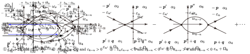
Figure 18: Feynman diagram of MT term in intrinsic Hall conductivity.

The MT term for intrinsic spin Hall conductivity is given by

$$\sigma_{xy}^{\mathrm{MT}}= \frac{e^{2}\hbar T}{64\pi m\xi_{\text{\scalebox{0.7}{$\mathrm{SC}$}}}^{2}(\lambda k_{\mathrm{F}})^{2}}\quantity[\real\psi\quantity(\frac{1}{2}+\frac{i\lambda k_{\mathrm{F}}}{2\pi T})-\psi\quantity(\frac{1}{2})]\ln\frac{1}{\epsilon}.$$ (126)

Figure 19 shows the profile of $\real\psi(1/2+ix)-\psi(1/2)$.

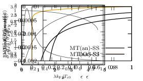
Figure 19: The profile of $\real\psi\quantity(1/2+ix)-\psi\quantity(1/2)$.

With use of $\real\psi(1/2+ix)-\psi(1/2)\approx 7\zeta(3)x^{2}$ for $x\ll 1$, we obtain

$$\sigma_{xy}^{\mathrm{MT}}= \frac{e^{2}}{16\pi\hbar}\frac{T}{\varepsilon_{\mathrm{F}}}\ln\frac{1}{\epsilon}$$ (127)

for $\lambda k_{\mathrm{F}}\ll T$.

V Discussion

V.1 Summary of the results for $D=2$

We summarize the results for $D=2$ case, where the spin Hall conductivity diverges in the limit $\epsilon\rightarrow+0$.

Table 1: Extrinsic spin Hall conductivity for $D=2$ in the dirty limit. The results are normalized by the spin Hall conductivity in the normal state ;$\sigma_{xy}^{\mathrm{SJ(normal)}}$ or $\sigma_{xy}^{\mathrm{SS(normal)}}$.

	side jump	skew scattering
AL / normal	$2\dfrac{T}{\varepsilon_{\mathrm{F}}}\ln\dfrac{1}{\epsilon}$	$4\dfrac{T}{\varepsilon_{\mathrm{F}}}\ln\dfrac{1}{\epsilon}$
DOS / normal	$-\dfrac{7\zeta(3)}{\pi^{3}}\dfrac{\hbar/\tau}{\varepsilon_{\mathrm{F}}}\ln\dfrac{1}{\epsilon}$	$-\dfrac{14\zeta(3)}{\pi^{3}}\dfrac{\hbar/\tau}{\varepsilon_{\mathrm{F}}}\ln\dfrac{1}{\epsilon}$
MT (reg) / normal	$0$	$\dfrac{7\zeta(3)}{\pi^{3}}\dfrac{\hbar/\tau}{\varepsilon_{\mathrm{F}}}\ln\dfrac{1}{\epsilon}$
MT (an) / normal	$0$	$-\dfrac{\pi}{8}\dfrac{\hbar/\tau}{\varepsilon_{\mathrm{F}}}\dfrac{1}{\epsilon-\gamma_{\varphi}}\ln\dfrac{\epsilon}{\gamma_{\varphi}}$

Table 2: Extrinsic spin Hall conductivity for $D=2$ in the clean limit. The results are normalized by the spin Hall conductivity in the normal state $\sigma_{xy}^{\mathrm{SJ(normal)}}$ or $\sigma_{xy}^{\mathrm{SS(normal)}}$.

	side jump	skew scattering
AL / normal	$2\dfrac{T}{\varepsilon_{\mathrm{F}}}\ln\dfrac{1}{\epsilon}$	$2\dfrac{T}{\varepsilon_{\mathrm{F}}}\ln\dfrac{1}{\epsilon}$
DOS / normal	$-\dfrac{2\pi^{3}}{7\zeta(3)}\dfrac{T}{\varepsilon_{\mathrm{F}}}\dfrac{T\tau}{\hbar}\ln\dfrac{1}{\epsilon}$	$-\dfrac{4\pi^{3}}{7\zeta(3)}\dfrac{T}{\varepsilon_{\mathrm{F}}}\dfrac{T\tau}{\hbar}\ln\dfrac{1}{\epsilon}$
MT (reg) / normal	$0$	$2\dfrac{T}{\varepsilon_{\mathrm{F}}}\ln\dfrac{1}{\epsilon}$
MT (an) / normal	$0$	$-\dfrac{\pi^{4}}{28\zeta(3)}\dfrac{T}{\varepsilon_{\mathrm{F}}}\dfrac{1}{\epsilon-\gamma_{\varphi}}\ln\dfrac{\epsilon}{\gamma_{\varphi}}$

Table 3: Intrinsic spin Hall conductivity via Rashba-type spin-orbit interaction for $\lambda k_{\mathrm{F}}\ll T$. The results are normalized by that in the normal state; $\sigma_{xy}^{\mathrm{(normal)}}=e^{2}/8\pi\hbar$ (Eq. (42)).

AL / normal	$\dfrac{1}{2}\dfrac{T}{\varepsilon_{\mathrm{F}}}\ln\dfrac{1}{\epsilon}$
DOS / normal	$-\dfrac{1}{4}\dfrac{T}{\varepsilon_{\mathrm{F}}}\ln\dfrac{1}{\epsilon}$
MT / normal	$\dfrac{1}{2}\dfrac{T}{\varepsilon_{\mathrm{F}}}\ln\dfrac{1}{\epsilon}$

In tables 1, 2, 3, we note two properties common in extrinsic and intrinsic effects. One is that the singularity in the AL terms is $\ln(1/\epsilon)$, which is weaker than the power-law singularity in the AL terms in electric conductivity. The power-counting argument is given in V.2. As another point, we notice that all contributions contain the factor $1/\varepsilon_{\mathrm{F}}$, which weakens the fluctuation effect. The origin of this factor is discussed in V.3.

Table 4: Dominant contribution in extrinsic spin Hall conductivity in the dirty limit.

	$\sigma_{xy}^{\mathrm{SJ(normal)}}\gg\sigma_{xy}^{\mathrm{SS(normal)}}$	$\sigma_{xy}^{\mathrm{SJ(normal)}}\ll\sigma_{xy}^{\mathrm{SS(normal)}}$
$\gamma_{\varphi}\ll 1$	DOS-SJ	MT(an)-SS
$\gamma_{\varphi}\gg 1$	DOS-SJ	DOS-SS + MT(reg) -SS

Table 5: Dominant contribution in extrinsic spin Hall conductivity in the clean limit.

	$\sigma_{xy}^{\mathrm{SJ(normal)}}\gg\sigma_{xy}^{\mathrm{SS(normal)}}$	$\sigma_{xy}^{\mathrm{SJ(normal)}}\ll\sigma_{xy}^{\mathrm{SS(normal)}}$
$\dfrac{T\tau}{\hbar}\ll\dfrac{1}{\epsilon-\gamma_{\varphi}}$	DOS-SJ	MT(an)-SS
$\dfrac{T\tau}{\hbar}\gg\dfrac{1}{\epsilon-\gamma_{\varphi}}$	DOS-SJ	DOS-SS

First, we discuss the extrinsic case. In tables 1 and 2, we see that there are three energy scales; $\varepsilon_{\mathrm{F}}$, $T$, $\hbar/\tau$. We summarize the dominant contribution in tables 4 and 5. In the dirty limit, the DOS terms with the side jump process is dominant when $\sigma_{xy}^{\mathrm{SJ(normal)}}\gg\sigma_{xy}^{\mathrm{SS(normal)}}$. When $\sigma_{xy}^{\mathrm{SJ(normal)}}\ll\sigma_{xy}^{\mathrm{SS(normal)}}$, either anomalous MT terms or the sum of the DOS term and the regular part of the MT terms is dominant, depending on the magnitude of $\gamma_{\varphi}$. In the clean limit, the DOS terms with side jump process is dominant when $\sigma_{xy}^{\mathrm{SJ(normal)}}\gg\sigma_{xy}^{\mathrm{SS(normal)}}$. When $\sigma_{xy}^{\mathrm{SJ(normal)}}\ll\sigma_{xy}^{\mathrm{SS(normal)}}$, either anomalous part of the MT term or the DOS term is dominant depending on relative magnitude of $T\tau/\hbar$ and $1/(\epsilon-\gamma_{\varphi})$. Both in the dirty and clean limits, dominant contributions have signs opposite to that in the normal state.

Figure 20: Estimate of fluctuation effect based on the parameters for Nb.

Figure 21: Estimate of fluctuation effect based on the parameters for clean Al, where skew scattering is considered to be dominant.

We give an estimate of dominant contribution in fluctuation effect based on the parameters for Nb and clean Al when $\gamma_{\varphi}\ll 1$ in figures 21 and 21. We have assumed in these estimations $\gamma_{\varphi}$ independent of temperature but in reality importance of temperature-dependence in $\gamma_{\varphi}\ll 1$ has been pointed out [49, 50].

Next, we discuss the intrinsic case. All terms are independent of $\lambda k_{\mathrm{F}}$ as in the normal state when $\lambda k_{\mathrm{F}}\ll T$, and thus a tiny Rashba-type spin-orbit interaction makes contribution of fluctuations finite.

Fluctuation effects on intrinsic spin Hall conductivity except for DOS term has the same sign as that in the normal state, in contrast to the extrinsic case. In ref. [43], the lowest order correction due to two-body repulsive interactions was found to suppress the intrinsic spin Hall conductivity in the two-dimensional Rashba model. The enhancement of spin Hall conductivity due to two-body attraction in the present paper and the suppression due to repulsion in ref. [43] seem consistent with each other.

V.2 Power-counting of singularity in the limit $\epsilon\to 0$

We first consider the origin of the singularity near $\epsilon\rightarrow+0$ by power counting argument. After that, we discuss the physical implication of this result.

Before considering the singularity of AL terms in the spin Hall conductivity, we first review the origin of the singularity in those terms in electric conductivity, which is given by

$$\sigma_{xx}^{\mathrm{AL}}\propto \frac{1}{i\omega}\quantity[\sum_{\bm{q}}\bm{q}^{2}T\sum_{\Omega_{k}}L(\bm{q},i\Omega_{k})L(\bm{q},i\Omega_{k}+i\omega_{\nu})B_{\mathrm{c}}(i\Omega_{k},i\omega_{\nu})^{2}]_{i\omega_{\nu}\to\hbar\omega\approx 0}.$$ (128)

In contrast to spin Hall conductivity, the spin current vertex $B_{\mathrm{s}}$ does not appear. The charge current vertex in the zero frequency limit $B_{\mathrm{c}}(0,0)$ is nonzero. We can thus replace $B_{\mathrm{c}}(i\Omega_{k},i\omega_{\nu})$ by $B_{\mathrm{c}}(0,0)$ and obtain

$$\sigma_{xx}^{\mathrm{AL}}\propto \frac{1}{i\omega}B_{\mathrm{c}}(0,0)^{2}\quantity[\sum_{\bm{q}}\bm{q}^{2}T\sum_{\Omega_{k}}L(\bm{q},i\Omega_{k})L(\bm{q},i\Omega_{k}+i\omega_{\nu})]_{i\omega_{\nu}\to\hbar\omega\approx 0}$$ (129)

$$\propto B_{\mathrm{c}}(0,0)^{2}\underbrace{\sum_{\bm{q}}\bm{q}^{2}}_{\epsilon^{(D+2)/2}}\int\underbrace{d\Omega}_{\epsilon}\underbrace{\coth(\frac{\Omega}{2T})}_{\epsilon^{-1}}\underbrace{\derivative{\Omega}}_{\epsilon^{-1}}[\imaginary\underbrace{L^{R}(\bm{q},\Omega)}_{\epsilon^{-1}}]^{2}$$ (130)

in order to extract the most diverging contribution $\epsilon\to 0$. Note that $\omega$-linear term comes from the fluctuation part, and $\Omega$-derivative of the fluctuation part appears in the last line.

We count the power of $\epsilon$ in Eq. (130). From the form of $L$, each quantity scales as $\Omega\propto\epsilon$ and $q\propto\epsilon^{1/2}$ and accordingly $\derivative{\Omega}\propto\epsilon^{-1}$, $L\propto\epsilon^{-1}$, $dq\;q^{D+1}\propto\epsilon^{(D+2)/2}$. The fluctuation propagator $L$ is appreciable when $\Omega/T\ll 1$, where we can replace $\coth(\Omega/2T)\approx(\Omega/2T)^{-1}$ thus $\coth(\Omega/2T)$ yields a factor of $\epsilon^{-1}$. Consequently, we see that $\sigma_{xx}^{\mathrm{AL}}\propto\epsilon^{D/2-2}$.

We turn to the AL terms in spin Hall conductivity. In the zero frequency limit, $B_{\mathrm{s}}(0,0)=0$ and the dominant contribution comes from the $\omega$-linear in $B_{\mathrm{s}}(i\Omega_{k},i\omega_{\nu})$ and we obtain

$$\sigma_{xy}^{\mathrm{AL}}\propto \underbrace{\sum_{\bm{q}}\bm{q}^{2}}_{\epsilon^{(D+2)/2}}\underbrace{L(\bm{q},0)^{2}}_{\epsilon^{-2}}B_{\mathrm{c}2}(0,0)\derivative{x}\quantity[B_{\mathrm{s}2}(-x,x)+B_{\mathrm{s}2}(0,x)]_{x=0},$$ (131)

where the derivative of $L$ does not appear but that of $B_{\mathrm{s}}$ does. $B_{\mathrm{s}}$ is regular in $\omega$ and thus derivative $B_{\mathrm{s}}$ does not yield any power of $\epsilon^{-1}$. As a result, $\sigma_{xy}^{\mathrm{AL}}\propto\epsilon^{0}$. The power-counting argument does not distinguish $\ln\epsilon$ from $\epsilon^{0}$ and thus this argument correctly accounts for singularity of $\sigma_{xy}^{\mathrm{AL}}$.

Next, we discuss the power of $\epsilon$ in the DOS terms and the MT terms. It suffices to consider the contribution from $\Omega_{k}=0$ in electric conductivity and spin Hall conductivity. Consequently, the singularities in both quantities are the same.

The power of $\epsilon$ comes only from $\sum_{\bm{q}}L(\bm{q},0)$ in the DOS terms(for extrinsic and intrinsic cases) and the MT terms for intrinsic case and the regular part of the MT terms for extrinsic case. $L\propto\epsilon^{-1}$, $\sum_{\bm{q}}\propto\int dqq^{D-1}\propto\epsilon^{D/2}$ and thus $\sigma_{xy}^{\mathrm{DOS}},\sigma_{xy}^{\mathrm{MT(reg)}}\propto\epsilon^{0}$, which is consistent with $\sigma_{xy}^{\mathrm{DOS}},\sigma_{xy}^{\mathrm{MT(reg)}}\propto\ln(1/\epsilon)$.

The power of $\epsilon$ comes only from $\sum_{\bm{q}}L(\bm{q},0)(\gamma_{\varphi}-\xi_{\text{\scalebox{0.7}{$\mathrm{SC}$}}}^{2}\bm{q}^{2})^{-1}$ in anomalous part of the MT terms for extrinsic case. $L\propto\epsilon^{-1}$, $\sum_{\bm{q}}\propto\int dqq^{D-1}\propto\epsilon^{D/2}$, $\xi_{\text{\scalebox{0.7}{$\mathrm{SC}$}}}^{2}q^{2}\propto\epsilon$ and thus $\sigma_{xy}^{\mathrm{MT(an)}}\propto(\gamma_{\varphi}-\epsilon)^{-1}$, which is consistent with $\sigma_{xy}^{\mathrm{MT(an)}}\propto(\gamma_{\varphi}-\epsilon)^{-1}\ln\epsilon$.

We have seen that the AL terms in spin Hall conductivity have weaker singularity than the AL terms in electric conductivity. The AL terms in electric conductivity represent the effect of transport carried by the dynamically fluctuating Cooper-pairs[36]; the effects of those terms can also be described by the time-dependent-Ginzburg-Landau theory, which is the effective theory for boson(Cooper pairs) obtained by integrating out the fermionic degrees of freedom. In the case of s-wave superconductors, however, the Cooper pairs carry electric charges but do not spin. Accordingly, the AL terms in the spin Hall conductivity represent a different physical process from that in electric conductivity. The $\omega$-linear term in the response function comes from the fluctuation propagator in the case of the AL terms in electric conductivity, while the $\omega$-linear term comes from the spin current vertex in the spin Hall conductivity. We could thus say that the AL terms in electric conductivity describe the dynamical effect of Cooper-pairs. In contrast, the AL terms in spin Hall conductivity come from the dynamical part of the spin current vertex with the static effect of fluctuating Cooper-pairs. This kind of dynamical aspect of the spin current vertex in the spin Hall effect has been pointed out in an earlier study[32], where the vortex spin Hall effect in the presence of magnetic field and spin accumulation is discussed.

Singularity in the DOS terms in spin Hall conductivity is the same as that in electric conductivity. This can be understood by recalling that the DOS terms represent the quasiparticle contribution. In this process, spin/charge is carried by quasiparticles. The presence of the fluctuating Cooper-pairs suppresses the density of states of the quasiparticles above the transition temperature[51, 52]. Thereby, electric conductivity is suppressed. The quasiparticles carry spin as well as charge and thus those terms for the spin Hall conductivity diverges in a way similar to electric conductivity.

V.3 Magnitude of spin Hall conductivity; $\epsilon$-independent factors

In this subsection, we discuss the other factor than $\epsilon$-dependence in spin Hall conductivity. In tables 1, 2, and 3, we notice the factor $\varepsilon_{\mathrm{F}}^{-1}$ in all cases. This factor reduces the effects of fluctuation on spin Hall conductivity. We will inspect the origin of this factor by counting the power of $k_{\mathrm{F}}$ in the expressions for spin Hall conductivity normalized by that in the normal state.

The charge current vertex and spin current vertex together yield $k_{\mathrm{F}}^{2}$ in the AL terms in the presence of side jump, and they do $k_{\mathrm{F}}^{4}$ in the AL terms in the presence of skew scattering. Expansion of Green function with respect to $\bm{q}$ gives $k_{\mathrm{F}}^{2}$. The sum of the product of the fluctuation propagators yields $\sum_{\bm{q}}\bm{q}^{2}L^{2}(\bm{q},0)\propto\xi_{\text{\scalebox{0.7}{$\mathrm{SC}$}}}^{-(D+2)}\propto k_{\mathrm{F}}^{-(D+2)}$. Those factors amount to $k_{\mathrm{F}}^{0}$ in $D=2$ for side jump and $k_{\mathrm{F}}^{2}$ for skew scattering. In the normal state, neither the factor $k_{\mathrm{F}}^{2}$ stemming from expansion of green function nor $k_{\mathrm{F}}^{-(D+2)}$ coming from the sum with respect to $\bm{q}$ exist. Consequently, the spin Hall conductivity in the normal state has one power of $\varepsilon_{\mathrm{F}}$ larger than the fluctuation conductivity in the AL terms in $D=2$. In the DOS terms and the MT terms, we do not expand the green function concerning $\bm{q}$ and thus the power of $k_{\mathrm{F}}$ coming from the spin current vertex and charge current vertex factor is the same as that in the normal state. In the DOS terms and the MT terms, the sum of fluctuation propagator yields $\sum_{\bm{q}}L(\bm{q},0)\propto\xi_{\text{\scalebox{0.7}{$\mathrm{SC}$}}}^{-D}\propto k_{\mathrm{F}}^{-D}$. By the last factor, the spin Hall conductivity in the normal state has a multiplicative factor $\varepsilon_{\mathrm{F}}$, compared to the fluctuation conductivity in the DOS terms and MT terms.

Namely, the integral $\sum_{\norm{\bm{q}}<\xi_{\text{\scalebox{0.7}{$\mathrm{SC}$}}}^{-1}}\bm{q}^{2}L^{2}(\bm{q},0)$ or $\sum_{\norm{\bm{q}}<\xi_{\text{\scalebox{0.7}{$\mathrm{SC}$}}}^{-1}}L(\bm{q},0)$ yields factor $1/\xi_{\text{\scalebox{0.7}{$\mathrm{SC}$}}}$ and reduces magnitude of the spin Hall conductivity. The small phase volume of $\bm{q}$ restricted by the condition $\norm{\bm{q}}<\xi_{\text{\scalebox{0.7}{$\mathrm{SC}$}}}^{-1}$ or the support of $L(\bm{q},0)$ implies that a limited number of electrons can contribute to the fluctuation part of the spin Hall conductivity. This fact reflects in additional factor $\varepsilon_{\mathrm{F}}^{-1}$ in fluctuation conductivity, compared to spin Hall conductivity in the normal state.

V.4 Relation to anomalous Hall effect

As mentioned in Sec. I, it is known that there is connection between extrinsic spin Hall effect and extrinsic anomalous Hall effect[9, 17, 37]. In this subsection, we discuss the relation to the reference [38], where the superconducting fluctuation on anomalous Hall effect was addressed.

The uniform component of the spin and charge current density operator can be written as Eqs. (12) and (15), respectively. These equations are identical except that (i) $\bm{j}_{\mathrm{s}}$ contains the factor $1/2$ (ii)$\sigma_{\alpha\beta}^{z}$ and $\delta_{\alpha\beta}$ are swapped. Therefore, the Feynman diagrams of the spin Hall effect and anomalous Hall effect become very similar. One of the differences is that diagrams of anomalous Hall effect contain an odd number of $\sigma_{\alpha\beta}^{z}$. In a ferromagnetic metal, physical quantities of up spin electron and down spin electron, such as density of states, have different values. Thus, we can incorporate the difference of the quantities into the coupling constant of spin-orbit interaction $\alpha_{\mathrm{so}}$ by taking an average of spin direction (see Eq. (2.7) in [38]).

From the above discussion, we can rewrite the results in this paper to the results in [38] by replacing the strength of spin-orbit interaction $\lambda_{0}^{2}$ to $8\alpha_{\mathrm{so}}/p_{\mathrm{F}}^{2}$. However, the procedures in this paper for extracting the most diverging term slightly differ from that in [38]. Because of this, the results in [38] are different from our results by a numerical factor.

Besides, diagram containing more fluctuation propagators have more factor of $\varepsilon_{\mathrm{F}}^{-1}$ as mentioned in the last of V.3. Li and Levchenko calculated the diagrams that contain more fluctuation propagators than diagrams in this paper and showed that these contributions have the factor of $\varepsilon_{\mathrm{F}}^{-2}$ (see Table 1 in [38]). The nonlinear fluctuation effects are more singular with $\epsilon$ than the lowest order contributions of the fluctuation effects and they are dominant when $\hbar/(\varepsilon_{\mathrm{F}}\tau)\ll\epsilon\ll\sqrt{\hbar/(\varepsilon_{\mathrm{F}}\tau)}$ in dirty 2D superconductors[38]. For simplicity, we restrict the the lowest order contributions of the fluctuation effects. This treatment is valid when $\sqrt{\hbar/(\varepsilon_{\mathrm{F}}\tau)}\ll\epsilon\ll 1$ in 2D dirty superconductors.

V.5 Future Issues

As we are motivated in the present study, the experiments by Jeon et al.[29] imply important roles of superconducting fluctuations in spin injection into superconductors or spin-charge conversion in superconductors above $T_{\rm c}$. As future issues, fluctuation effects on spin-pumping, spin-Seebeck, and charge-imbalance related to spin injection into superconductors are worthwhile to address.

Spin injection from magnets to metals can be driven by electromagnetic field (spin pumping) or thermal gradient at the interface (spin-Seebeck effect). While both subjects for superconductors have been addressed within the mean field theory[25, 26], fluctuation effects on these effects have yet to be considered. As developed in [25, 26], the spin currents injected via spin-pumping and spin-Seebeck effect depend on local magnetic susceptibility $\chi_{\mathrm{loc}}^{R}(\omega)$. In the limit $\omega\to 0$, the AL process vanishes as it occurs in spin Hall conductivity. When the dephasing is weak or moderate, the MT term becomes dominant and is proportional to $(\epsilon-\gamma_{\varphi})^{-1}\ln(\epsilon/\gamma_{\varphi})$ when $T\tau/\hbar\ll 1$ or $1\ll T\tau/\hbar\ll 1/\sqrt{\epsilon}$, and $\epsilon^{-1/2}\ln(T\tau\sqrt{\epsilon})$ when $1\ll 1/\sqrt{\epsilon}\ll T\tau/\hbar$[53]. Consideration of fluctuation effects on $\chi_{\mathrm{loc}}^{R}(\omega)$ for finite $\omega\neq 0$ will reveal fluctuation effects on spin-Seebeck and spin-pumping effects.

Charge imbalance is another issue to be addressed. In nonequilibrium steady states in superconductors, quasiparticle density can deviate from equilibrium value, and excess or depletion of quasiparticle density is compensated by that of Cooper-pairs by charge neutrality condition. Spatial variation of Cooper-pair density (and hence that of the chemical potential of Cooper-pairs) induces the electric field so that electrochemical potential for Cooper-pairs is spatially uniform. The inverse spin Hall voltage measured in experiments in [29] is considered to be a consequence of this charge imbalance caused by a spin-charge conversion of quasiparticles in the superconductor. Charge-imbalance has been discussed theoretically in the Boltzmann-type transport theory. It is appropriate to deal with the charge imbalance within the Green function formalism, to incorporate superconducting fluctuations.

The spin Hall effect in the normal state in Nb has been attributed to intrinsic effect [54, 55] based on a semi-quantitative model reflecting the multi-orbital electronic band structure. For a quantitative account for the experiments by Jeon et al. [29], a theoretical study on the fluctuation effects based on a realistic model is desirable. In future research developed in this direction, the fluctuation effects on spin transport in the simple models used in the present paper will serve as a basis for understanding the results of realistic models and experiments.

VI Conclusion

In this paper, we theoretically study the effects of superconducting fluctuations on extrinsic spin Hall effects in two- and three-dimensional electron gas and intrinsic spin Hall effects in the two-dimensional Rashba model. The AL, DOS, MT terms have logarithmic divergence $\ln\epsilon$ in the limit $\epsilon=(T-T_{\mathrm{c}})/T_{\mathrm{c}}\rightarrow+0$ in two-dimensional systems for both extrinsic and intrinsic spin Hall effects except the MT terms in extrinsic effect, which are proportional to $(\epsilon-\gamma_{\varphi})^{-1}\ln\epsilon$ with a cutoff $\gamma_{\varphi}$ in two-dimensional systems. The fluctuation correction to the extrinsic spin Hall effect has an opposite sign to that in the normal state and suppresses the spin Hall effect. The correction to the intrinsic spin Hall effect has the same sign as that in the normal state and thus enhances the spin Hall effect. The study of fluctuation effects on spin injection to superconductors based on more realistic models as well as the simple models is an important issue in the future.

VII Acknowledgements

This work was supported by JSPS KAKENHI Grant Number 19K05253 and 20K20891. AW and YK thank Yuta Suzuki for his comments on the intrinsic spin Hall effect in the Rashba model.

Appendix: List of Symbols

$T$

temperature, which has the dimension of energy in the present paper because we set $k_{\mathrm{B}}=1$.

$\beta$

$1/T$ inverse temperature.

$T_{\mathrm{c}}$

transition temperature.

$\mu$

chemical potential unless it is used as the superscript/subscript.

$\varepsilon_{\bm{k}}$

$\varepsilon_{\bm{k}}\equiv\hbar^{2}\bm{k}^{2}/2m$.

$V$

volume of system.

$\mathcal{V}(\bm{r})$

potential of impurities. $\mathcal{V}(\bm{r})=\sum_{i}\mathcal{V}_{\mathrm{single}}(\bm{r}-\bm{R}_{i})$, where $\mathcal{V}_{\mathrm{single}}(\bm{r})$ is potential of single impurity and $\bm{R}_{i}$ is position of impurities.

$v_{0}$

$v_{0}\equiv\int d\bm{r}\mathcal{V}_{\mathrm{single}}(\bm{r})$.

$n_{\mathrm{i}}$

density of impurities.

$\bm{A}$

vector potential.

$e$

electric charge unit, $e>0$.

$\bm{\sigma}$

the Pauli matrices. $\bm{\sigma}={}^{t}(\sigma^{x},\sigma^{y},\sigma^{z})$.

$\lambda_{0}$

coupling constant of spin-orbit interaction in extrinsic spin Hall effect.

$\lambda$

coupling constant of spin-orbit interaction in intrinsic spin Hall effect. $\lambda$ is different from $\lambda_{0}$ for extrinsic spin Hall effect.

$m$

electron mass.

$\anticommutator{\cdots}{\cdots}$

anticommutator.

$\hat{\bm{z}}$

unit vector along $z$-direction.

$\psi_{\sigma}(\bm{r})$

annihilation operator of electron with $z$-component of spin $\sigma$.

$\psi_{\sigma\bm{k}}$

Fourier transform of $\psi_{\sigma}(\bm{r})$.

$c_{\bm{k}\alpha}$

annihilation operator of one-particle state with wavenumber $\bm{k}$ in the band $\alpha$. It is defined by Eq. (29).

$j_{\mathrm{s}}$

spin current density operator or the uniform component of Fourier transform of the spin current density operator.

$j_{\mathrm{c}}$

charge current density operator or the uniform component of Fourier transform of the charge current density operator.

$\varepsilon_{n}$

Fermionic Matsubara frequency. $\varepsilon_{n}\equiv(2n+1)\pi T\quad(n\in\mathbb{Z})$.

$\omega_{n}$

Bosonic Matsubara frequency (external frequency). $\omega_{n}\equiv 2n\pi T\quad(n\in\mathbb{Z})$.

$\Omega_{n}$

Bosonic Matsubara frequency (internal frequency). $\Omega_{n}\equiv 2n\pi T\quad(n\in\mathbb{Z})$.

$\widetilde{\varepsilon}_{n}$

$\widetilde{\varepsilon}_{n}\equiv\varepsilon_{n}+(\hbar/2\tau)\operatorname{sign}(\varepsilon_{n})$.

$\Phi_{\mu\nu}(\bm{q},i\omega_{\nu})$

spin current-charge current response function with the wavevector $\bm{q}$ and frequency, $i\omega_{\nu}$ carried by an external field.

$\mathcal{G}_{\alpha}(\bm{k},i\varepsilon_{n})$

green function, which is defined by Eq. (21) for extrinsic spin Hall effect and by Eq. (41) for intrinsic spin Hall effect.

$\tau$

impurity scattering time.

$N(0)$

density of states at the Fermi surface.

$D$

spatial dimension. $D=2$ or $D=3$.

$\varepsilon_{\mathrm{F}}$

Fermi energy.

$k_{\mathrm{F}}$

Fermi wavevector.

$v_{\mathrm{F}}$

Fermi velocity.

$F(z)$

$F(z)\equiv 1/(e^{\beta z}+1)$.

$L(\bm{q},i\Omega_{k})$

propagator of superconducting fluctuation, fluctuation propagator.

$C(\bm{q},\varepsilon_{1},\varepsilon_{2})$

Cooperon.

$\omega_{\mathrm{D}}$

Debye frequency.

$\expectationvalue{\cdots}_{\mathrm{F.S.}}$

angular average over the fermi surface.

$\psi(z)$

diGamma function. $\psi(z)\equiv\derivative{z}\ln\Gamma(z)=\lim_{n_{\mathrm{c}}\to\infty}[-\sum_{n=0}^{n_{\mathrm{c}}-1}(n+z)^{-1}+\ln n_{\mathrm{c}}]$. The $n$-th order derivative of $\psi(z)$ is denoted by $\psi^{(n)}(z)$, which is called polyGamma function.

$C_{\mathrm{Euler}}$

Euler-Mascheroni constant. $C_{\mathrm{Euler}}=0.577\cdots$.

$\gamma_{\mathrm{E}}$

$\gamma_{\mathrm{E}}\equiv e^{C_{\mathrm{Euler}}}$.

$\epsilon$

$\epsilon\equiv\ln(T/T_{\mathrm{c}})$, which becomes $\epsilon\approx(T-T_{\mathrm{c}})/T_{\mathrm{c}}$ near $T\approx T_{\mathrm{c}}$.

$\xi_{\text{\scalebox{0.7}{$\mathrm{SC}$}}}$

$\xi(T)\sqrt{\epsilon}$ with the coherence length $\xi(T)$ in Ginzburg-Landau theory. In the present paper, we call $\xi_{\text{\scalebox{0.7}{$\mathrm{SC}$}}}$ coherence length. It is defined by Eq. (50).

$\mathcal{D}$

diffusion constant defined by Eq. (50).

$\mathcal{B}(\bm{q},i\Omega_{k},i\omega_{\nu})$

triangular part containing spin current/charge current vertex.

$\tau_{\varphi}$

phase-breaking time, which is necessary to introduce as a cutoff for extrinsic spin Hall effect in two-dimension systems as well as for electric conductivity.

$\gamma_{\varphi}$

dimensionless parameter for phase breaking $\gamma_{\varphi}\equiv\pi\hbar/8T\tau_{\varphi}$.

$\zeta(x)$

zeta function. $\zeta(3)=1.202\cdots$.

$\zeta_{\rm s}$

$\frac{e\hbar\lambda_{0}^{2}n_{\mathrm{i}}v_{0}^{2}}{4m}\frac{k_{\mathrm{F}}^{2}}{D}\quantity(N(0))^{2}$.

$\zeta^{\prime}_{\rm s}$

$\frac{e\hbar^{3}\lambda_{0}^{2}n_{\mathrm{i}}v_{0}^{3}}{4m^{2}}\frac{k_{\mathrm{F}}^{4}}{D^{2}}\quantity(N(0))^{3}$.

$\zeta_{\rm c}$

$\frac{2e\hbar^{3}}{m^{2}}\frac{k_{\mathrm{F}}^{2}}{D}N(0)$.

References

- Tedrow and Meservey [1971] P. M. Tedrow and R. Meservey, Spin-Dependent Tunneling into Ferromagnetic Nickel, Phys. Rev. Lett. 26, 192 (1971).
- Aronov [1976] A. G. Aronov, Spin injection in metals and polarization of nuclei, Pis’ma Zh. Eksp. Teor. Fiz. 24, 37 (1976).
- Johnson and Silsbee [1985] M. Johnson and R. H. Silsbee, Interfacial charge-spin coupling: Injection and detection of spin magnetization in metals, Phys. Rev. Lett. 55, 1790 (1985).
- Dyakonov and Perel [1971] M. I. Dyakonov and V. I. Perel, Current-induced spin orientation of electrons in semiconductors, Phys. Lett. A 35, 459 (1971).
- Hirsch [1999] J. E. Hirsch, Spin Hall Effect, Phys. Rev. Lett. 83, 1834 (1999).
- Zhang [2000] S. Zhang, Spin Hall Effect in the Presence of Spin Diffusion, Phys. Rev. Lett. 85, 393 (2000).
- Takahashi and Maekawa [2002] S. Takahashi and S. Maekawa, Hall Effect Induced by a Spin-Polarized Current in Superconductors, Phys. Rev. Lett. 88, 116601 (2002).
- Engel et al. [2005] H.-A. Engel, B. I. Halperin, and E. I. Rashba, Theory of Spin Hall Conductivity in -Doped GaAs, Phys. Rev. Lett. 95, 166605 (2005).
- Tse and Das Sarma [2006] W.-K. Tse and S. Das Sarma, Spin Hall Effect in Doped Semiconductor Structures, Phys. Rev. Lett. 96, 056601 (2006).
- Murakami et al. [2003] S. Murakami, N. Nagaosa, and S.-C. Zhang, Dissipationless Quantum Spin Current at Room Temperature, Science 301, 1348 (2003).
- Sinova et al. [2004] J. Sinova, D. Culcer, Q. Niu, N. A. Sinitsyn, T. Jungwirth, and A. H. MacDonald, Universal Intrinsic Spin Hall Effect, Phys. Rev. Lett. 92, 126603 (2004), arXiv:0307663 [cond-mat] .
- Kato et al. [2004] Y. K. Kato, R. C. Myers, A. C. Gossard, and D. D. Awschalom, Observation of the Spin Hall Effect in Semiconductors, Science 306, 1910 (2004).
- Wunderlich et al. [2005] J. Wunderlich, B. Kaestner, J. Sinova, and T. Jungwirth, Experimental Observation of the Spin-Hall Effect in a Two-Dimensional Spin-Orbit Coupled Semiconductor System, Phys. Rev. Lett. 94, 047204 (2005), arXiv:0410295 [cond-mat] .
- Valenzuela and Tinkham [2006] S. O. Valenzuela and M. Tinkham, Direct electronic measurement of the spin Hall effect, Nature (London) 442, 176 (2006), arXiv:0605423 [cond-mat] .
- Saitoh et al. [2006] E. Saitoh, M. Ueda, H. Miyajima, and G. Tatara, Conversion of spin current into charge current at room temperature: Inverse spin-Hall effect, Appl. Phys. Lett. 88, 182509 (2006).
- Sinova et al. [2006] J. Sinova, S. Murakami, S.-Q. Shen, and M.-S. Choi, Spin-Hall effect: Back to the beginning at a higher level, Solid State Commun. 138, 214 (2006), arXiv:0512054 [cond-mat] .
- Sinova et al. [2015] J. Sinova, S. O. Valenzuela, J. Wunderlich, C. H. Back, and T. Jungwirth, Spin Hall effects, Rev. Mod. Phys. 87, 1213 (2015).
- Edelstein [1990] V. Edelstein, Spin polarization of conduction electrons induced by electric current in two-dimensional asymmetric electron systems, Solid State Commun. 73, 233 (1990).
- Ganichev et al. [2002] S. D. Ganichev, E. L. Ivchenko, V. V. Bel’kov, S. A. Tarasenko, M. Sollinger, D. Weiss, W. Wegscheider, and W. Prettl, Spin-galvanic effect, Nature (London) 417, 153 (2002).
- Yang et al. [2021] G. Yang, C. Ciccarelli, and J. W. A. Robinson, Boosting spintronics with superconductivity, APL Mater. 9, 050703 (2021).
- Zhao and Hershfield [1995] H. L. Zhao and S. Hershfield, Tunneling, relaxation of spin-polarized quasiparticles, and spin-charge separation in superconductors, Phys. Rev. B 52, 3632 (1995).
- Hübler et al. [2012] F. Hübler, M. J. Wolf, D. Beckmann, and H. v. Löhneysen, Long-Range Spin-Polarized Quasiparticle Transport in Mesoscopic Al Superconductors with a Zeeman Splitting, Phys. Rev. Lett. 109, 207001 (2012), arXiv:1208.0717 .
- Wakamura et al. [2014] T. Wakamura, N. Hasegawa, K. Ohnishi, Y. Niimi, and Y. Otani, Spin Injection into a Superconductor with Strong Spin-Orbit Coupling, Phys. Rev. Lett. 112, 036602 (2014).
- Wakamura et al. [2015] T. Wakamura, H. Akaike, Y. Omori, Y. Niimi, S. Takahashi, A. Fujimaki, S. Maekawa, and Y. Otani, Quasiparticle-mediated spin Hall effect in a superconductor, Nat. Mater. 14, 675 (2015).
- Inoue et al. [2017] M. Inoue, M. Ichioka, and H. Adachi, Spin pumping into superconductors: A new probe of spin dynamics in a superconducting thin film, Phys. Rev. B 96, 024414 (2017), arXiv:1704.04303 .
- Kato et al. [2019] T. Kato, Y. Ohnuma, M. Matsuo, J. Rech, T. Jonckheere, and T. Martin, Microscopic theory of spin transport at the interface between a superconductor and a ferromagnetic insulator, Phys. Rev. B 99, 144411 (2019), arXiv:1901.02440 .
- Ojajärvi et al. [2021] R. Ojajärvi, T. T. Heikkilä, P. Virtanen, and M. A. Silaev, Giant enhancement to spin battery effect in superconductor/ferromagnetic insulator systems, Phys. Rev. B 103, 224524 (2021).
- Jeon et al. [2018] K.-R. Jeon, C. Ciccarelli, H. Kurebayashi, J. Wunderlich, L. F. Cohen, S. Komori, J. W. A. Robinson, and M. G. Blamire, Spin-Pumping-Induced Inverse Spin Hall Effect in Bilayers and its Strong Decay Across the Superconducting Transition Temperature, Phys. Rev. Appl. 10, 014029 (2018), arXiv:1805.00730 .
- Jeon et al. [2020] K.-R. Jeon, J.-C. Jeon, X. Zhou, A. Migliorini, J. Yoon, and S. S. P. Parkin, Giant Transition-State Quasiparticle Spin-Hall Effect in an Exchange-Spin-Split Superconductor Detected by Nonlocal Magnon Spin Transport, ACS Nano 14, 15874 (2020).
- Kontani et al. [2009] H. Kontani, J. Goryo, and D. S. Hirashima, Intrinsic Spin Hall Effect in the -Wave Superconducting State: Analysis of the Rashba Model, Phys. Rev. Lett. 102, 086602 (2009), arXiv:0806.4237 .
- Takahashi and Maekawa [2012] S. Takahashi and S. Maekawa, Spin Hall Effect in Superconductors, Jpn. J. Appl. Phys. 51, 010110 (2012).
- Taira et al. [2021] T. Taira, Y. Kato, M. Ichioka, and H. Adachi, Spin Hall effect generated by fluctuating vortices in type-II superconductors, Phys. Rev. B 103, 134417 (2021), arXiv:2012.03471 .
- Aslamasov and Larkin [1968] L. G. Aslamasov and A. I. Larkin, The influence of fluctuation pairing of electrons on the conductivity of normal metal, Phys. Lett. A 26, 238 (1968).
- Maki [1968] K. Maki, The critical fluctuation of the order parameter in type-II superconductors, Prog. Theor. Phys. 39, 897 (1968).
- Thompson [1970] R. S. Thompson, Microwave, Flux Flow, and Fluctuation Resistance of Dirty Type-II Superconductors, Phys. Rev. B 1, 327 (1970).
- Larkin and Varlamov [2009] A. Larkin and A. Varlamov, Oxford Univ. Press (Oxford University Press, New York, 2009).
- Nagaosa et al. [2010] N. Nagaosa, J. Sinova, S. Onoda, A. H. MacDonald, and N. P. Ong, Anomalous Hall effect, Rev. Mod. Phys. 82, 1539 (2010), arXiv:0904.4154 .
- Li and Levchenko [2020] S. Li and A. Levchenko, Fluctuational anomalous Hall and Nernst effects in superconductors, Ann. Phys. (N. Y). 417, 168137 (2020), arXiv:2002.08364 .
- Inoue et al. [2004] J.-i. Inoue, G. E. W. Bauer, and L. W. Molenkamp, Suppression of the persistent spin Hall current by defect scattering, Phys. Rev. B 70, 041303 (2004).
- Schliemann and Loss [2004] J. Schliemann and D. Loss, Dissipation effects in spin-Hall transport of electrons and holes, Phys. Rev. B 69, 165315 (2004).
- Mishchenko et al. [2004] E. G. Mishchenko, A. V. Shytov, and B. I. Halperin, Spin Current and Polarization in Impure Two-Dimensional Electron Systems with Spin-Orbit Coupling, Phys. Rev. Lett. 93, 226602 (2004).
- Rashba [2004] E. I. Rashba, Spin currents, spin populations, and dielectric function of noncentrosymmetric semiconductors, Phys. Rev. B 70, 161201 (2004).
- Dimitrova [2005] O. V. Dimitrova, Spin-Hall conductivity in a two-dimensional Rashba electron gas, Phys. Rev. B 71, 245327 (2005).
- Murakami [2006] S. Murakami, Intrinsic Spin Hall Effect, in Adv. Solid State Phys., edited by B. Kramer (Springer Berlin Heidelberg, Berlin/Heidelberg, 2006) pp. 197–209.
- Raimondi et al. [2012] R. Raimondi, P. Schwab, C. Gorini, and G. Vignale, Spin-orbit interaction in a two-dimensional electron gas: A SU(2) formulation, Ann. Phys. (Leipzig) 524, 10.1002/andp.201100253 (2012), arXiv:1110.5279 .
- Shekhter et al. [2005] A. Shekhter, M. Khodas, and A. M. Finkel’stein, Chiral spin resonance and spin-Hall conductivity in the presence of the electron-electron interactions, Phys. Rev. B 71, 165329 (2005).
- Gor’kov and Rashba [2001] L. P. Gor’kov and E. I. Rashba, Superconducting 2D System with Lifted Spin Degeneracy: Mixed Singlet-Triplet State, Phys. Rev. Lett. 87, 037004 (2001), arXiv:0103449 [cond-mat] .
- Edelstein [1989] V. M. Edelstein, Characteristics of the Cooper pairing in two-dimensional noncentrosymmetric electron systems, Zh. Eksp. Teor. Fiz. 95, 2151 (1989).
- Mori et al. [1990] N. Mori, T. Kobayashi, T. Shimizu, and H. Ozaki, Paraconductivity and Temperature-Dependent Pair-Breaking Parameter in Superconducting Niobium Thin Films, J. Phys. Soc. Jpn. 59, 2205 (1990).
- Craven et al. [1973] R. A. Craven, G. A. Thomas, and R. D. Parks, Fluctuation-Induced Conductivity of a Superconductor above the Transition Temperature, Phys. Rev. B 7, 157 (1973).
- Di Castro et al. [1990] C. Di Castro, R. Raimondi, C. Castellani, and A. A. Varlamov, Superconductive fluctuations in the density of states and tunneling resistance in high- superconductors, Phys. Rev. B 42, 10211 (1990).
- Abrahams et al. [1970] E. Abrahams, M. Redi, and J. W. F. Woo, Effect of Fluctuations on Electronic Properties above the Superconducting Transition, Phys. Rev. B 1, 208 (1970).
- Randeria and Varlamov [1994] M. Randeria and A. A. Varlamov, Effect of superconducting fluctuations on spin susceptibility and NMR relaxation rate, Phys. Rev. B 50, 10401 (1994).
- Morota et al. [2011] M. Morota, Y. Niimi, K. Ohnishi, D. H. Wei, T. Tanaka, H. Kontani, T. Kimura, and Y. Otani, Indication of intrinsic spin Hall effect in and transition metals, Phys. Rev. B 83, 174405 (2011), arXiv:1008.0158 .
- Tanaka et al. [2008] T. Tanaka, H. Kontani, M. Naito, T. Naito, D. S. Hirashima, K. Yamada, and J. Inoue, Intrinsic spin Hall effect and orbital Hall effect in and transition metals, Phys. Rev. B 77, 165117 (2008), arXiv:0711.1263 .