Functional Linear Regression of Cumulative Distribution Functions

Abstract

The estimation of cumulative distribution functions (CDFs) is an important learning task with a great variety of downstream applications, such as risk assessments in predictions and decision making. In this paper, we study functional regression of contextual CDFs where each data point is sampled from a linear combination of context dependent CDF basis functions. We propose functional ridge-regression-based estimation methods that estimate CDFs accurately everywhere. In particular, given $n$ samples with $d$ basis functions, we show estimation error upper bounds of $\widetilde{O}(\sqrt{d/n})$ for fixed design, random design, and adversarial context cases. We also derive matching information theoretic lower bounds, establishing minimax optimality for CDF functional regression. Furthermore, we remove the burn-in time in the random design setting using an alternative penalized estimator. Then, we consider agnostic settings where there is a mismatch in the data generation process. We characterize the error of the proposed estimators in terms of the mismatched error, and show that the estimators are well-behaved under model mismatch. Finally, to complete our study, we formalize infinite dimensional models where the parameter space is an infinite dimensional Hilbert space, and establish self-normalized estimation error upper bounds for this setting.

1 Introduction

Estimating cumulative distribution functions (CDF) of random variables is a salient theoretical problem that underlies the study of many real-world phenomena. For example, Huang et al. (2021) and Leqi et al. (2022) recently showed that estimating CDFs is sufficient for risk assessment, thereby making CDF estimation a key building block for such decision-making problems. In a similar vein, it is known that CDFs can also be used to directly compute distorted risk functions (Wirch and Hardy, 2001), coherent risks (Artzner et al., 1999), spectral risks (Acerbi, 2002), value-at-risk, conditional value-at-risk, and mean-variance (Cassel et al., ; Sani et al., 2013; Vakili and Zhao, 2015; Zimin et al., 2014), and cumulative prospect theory risks (Prashanth et al., 2016). Furthermore, CDFs are also useful in calculating various risk functionals appearing in insurance premium design, portfolio design, behavioral economics, behavioral finance, and healthcare applications (Sharpe, 1966; Rockafellar et al., 2000; Krokhmal, 2007; Shapiro et al., 2014; Acerbi, 2002; Prashanth et al., 2016; Jie et al., 2018; Wong et al., 2022). Given the broad utility of estimating CDFs, there is a vast (and fairly classical) literature that tries to understand this problem.

In particular, the renowned Glivenko–Cantelli theorem (Cantelli, 1933; Glivenko, 1933) (also known as the fundamental theorem of mathematical statistics, Devroye et al., 2013) states that given some independent samples of a random variable, one can construct a consistent estimator for its CDF. Tight non-asymptotic sample complexity rates for such estimation using the Kolmogorov-Smirnov (KS) distance as the loss have also been established in the literature (Cantelli, 1933; Glivenko, 1933; Dvoretzky et al., 1956; Massart, 1990). However, these results are all limited to the setting of a single random variable. In contrast, many modern learning problems, such as doubly-robust estimators in contextual bandits, treatment effects, and Markov decision processes (Huang et al., 2021; Kallus et al., 2019; Huang et al., 2022), require us to simultaneously learn the CDFs of potentially infinitely many random variables from limited data. Hence, the classical results on CDF estimation do not address the needs of such emerging learning applications.

Contributions.

In this work, as a first step towards developing general CDF estimation methods that fulfill the needs of the aforementioned learning problems, we study functional linear regression of CDFs, where samples are generated from CDFs that are linear (or convex) combinations of context-dependent CDF bases. As our main contribution, we define both least-squares regression and ridge regression estimators for the unknown linear weight parameter, and establish corresponding estimation error bounds for the fixed design, random design, adversarial, and self-normalized settings. In particular, given $n$ samples with $d$ CDF bases, we prove estimation error upper bounds that scale like $\widetilde{O}(\sqrt{d/n})$ (neglecting sub-dominant factors). Our results achieve the same problem-dependent scaling as in canonical finite dimensional linear regression (Abbasi-Yadkori et al., 2011b, a; Peña et al., 2008; Hsu et al., 2012b). On the other hand, our results specialize the functional regression setting of Benatia et al. (2017); Wang et al. (2020) to CDF estimation, where minimal assumptions are made on the data generation process. Moreover, we also derive $\Omega(\sqrt{d/n})$ information theoretic lower bounds for functional linear regression of CDFs. This establishes minimax estimation rates of $\widetilde{\Theta}(\sqrt{d/n})$ for the CDF functional regression problem. We later show that this result directly implies the concentration of CDFs in Kolmogorov-Smirnov (KS) distance. We also propose a new penalized estimator that theoretically eliminates the requirement on the burn-in time of sample size in the random design setting. Then, we consider agnostic settings where there is a mismatch between our linear model and the actual data generation process. We characterize the estimation error of the proposed estimator in terms of the mismatch error, and demonstrate that the estimator is well-behaved under model mismatch. To complete our study, we generalize the parameter space in the linear model from finite-dimensional Euclidean spaces to general infinite-dimensional Hilbert spaces, extend the ridge regression estimator to the infinite-dimensional model with proper regularization, and establish a corresponding self-normalized estimation error upper bound which immediately recovers our previous $\widetilde{O}(\sqrt{d/n})$ upper bound when the parameter space is restricted to be $d$-dimensional. Finally, we present numerical simulation results for a few synthetic and controlled experiments to illustrate the performance of our estimation methods.

It is worth mentioning that a complementary approach to the proposed CDF regression framework is quantile regression (Koenker and Bassett Jr, 1978). Although quantile regression may appear to be closely related to CDF regression at first glance, the two problems have very different flavors. Indeed, unlike CDFs, quantiles are not sufficient for law invariant risk assessment. Furthermore, due to their infinite range, quantile estimation is quite challenging, resulting in analyses that only consider pointwise estimation (Takeuchi et al., 2006). Perhaps more importantly, quantile regression can be ill-posed in many machine learning settings. For example, quantiles are not estimatable in decision-making problems and games with mixed random variables (which take both discrete and continuous values). For these reasons, our focus in this paper will be on CDF regression.

Outline.

We briefly outline the rest of the paper. Notation and formal setup for our problem are given in Section 2. We propose our estimation paradigm and analyze its theoretical performance in Section 3. We derive corresponding lower bounds on the estimation error of the problem in Section 4. We establish upper bounds on the estimation error under the existence of a mismatch in our proposed model in Section 5. We generalize the problem from estimating finite dimensional parameters to estimating infinite dimensional parameters, extend our estimation paradigm to this infinite dimensional setting, and prove an upper bound on estimation error in Section 6. Proofs of the main theoretical results in Sections 3, 4, and 6 are presented in Sections 7, 8, and 9, respectively. Numerical simulation results are displayed in Section 10. Conclusions are drawn and future research directions are suggested in Section 11. All the remaining proofs are presented in the appendices.

2 Preliminaries

In this section, we introduce the notation used in the paper and set up the learning problem of contextual CDF regression.

Notation.

Let $\mathbb{N}$ denote the set of positive integers. For any $n\in\mathbb{N}$, let $[n]$ denote the set $\{1,\dots,n\}$. For any measure space $(\Omega,\mathcal{F},\mathfrak{m})$, define the Hilbert space $\mathcal{L}^{2}(\Omega,\mathfrak{m}):=\{f:\Omega\rightarrow\mathbb{R}\ \big{|}\ \int_{\Omega}|f|^{2}d\mathfrak{m}<\infty\}$ with $\mathcal{L}^{2}$-norm $\|f\|_{\mathcal{L}^{2}(\Omega,\mathfrak{m})}:=\sqrt{\int_{\Omega}|f|^{2}d\mathfrak{m}}$ for $f\in\mathcal{L}^{2}(\Omega,\mathfrak{m})$. For any positive definite matrix $A\in\mathbb{R}^{d\times d}$, define $\|\cdot\|_{A}$ to be the weighted $\ell^{2}$-norm in $\mathbb{R}^{d}$ induced by $A$, i.e., $\|x\|_{A}=\sqrt{x^{\top}Ax}$ for $x\in\mathbb{R}^{d}$. For the standard Euclidean (or $\ell^{2}$-) norm $\|\cdot\|_{I_{d}}$, where $I_{d}$ denotes the $d\times d$ identity matrix, we omit the subscript $I_{d}$ and simply write $\|\cdot\|$. For any square matrix $A$, let $\mu_{\min}(A)$ denote the smallest eigenvalue of $A$, $\mu_{\max}(A)$ denote the largest eigenvalue of $A$ and $\|A\|_{2}$ denote the spectral norm of the matrix $A$, i.e., $\|A\|_{2}:=\sqrt{\mu_{\max}(A^{\top}A)}$. Let $\textup{KS}(F_{1},F_{2}):=\sup_{x\in\mathbb{R}}|F_{1}(x)-F_{2}(x)|$ denote the KS distance between two CDFs $F_{1}$ and $F_{2}$. Finally, let $\mathbbm{1}\{\cdot\}$ denote the indicator function. More technical notation dealing with measurability issues is provided at the beginning of Section 7.

Problem setup.

In this paper, we consider the problem of functional linear regression of CDFs. To define this problem, let $\mathcal{X}$ denote the context space, and let $F(x,\cdot):\mathbb{R}\rightarrow[0,1]$ be the CDF of some $\mathbb{R}$-valued random variable for any $x\in\mathcal{X}$. We assume that $\mathcal{X}$ is a Polish space throughout the paper. For a context $x\in\mathcal{X}$, we observe a sample $y$ from its corresponding CDF $F(x,\cdot)$. We next summarize two schemes to generate $(x,y)$ samples:

• Scheme I (Adversarial). For each $j\in\mathbb{N}$, an adversary picks $x^{(j)}\in\mathcal{X}$ (either deterministically or randomly) in an adaptive way given knowledge of the previous $y^{(i)}$’s for $i<j$, and then $y^{(j)}\in\mathbb{R}$ is sampled from $F(x^{(j)},\cdot)$. This includes the canonical fixed design setting as a special case, where all $x^{(j)}$’s are fixed a priori without knowledge of $y^{(j)}$’s.

• Scheme II (Random). For each $j\in\mathbb{N}$, $x^{(j)}\in\mathcal{X}$ is sampled from some probability distribution $P_{X}^{(j)}$ on $\mathcal{X}$ independently, and then $y^{(j)}\in\mathbb{R}$ is sampled from $F(x^{(j)},\cdot)$ independently. This is commonly known as the random design setting in the regression context.

Scheme I and Scheme II generalize the assumptions of the data generation process in canonical ridge regression in Abbasi-Yadkori et al. (2011a) and Hsu et al. (2012b) to the problem of CDF estimation, respectively. Note that although the random design setting in Scheme II is a special case of Scheme I, we emphasize it because it has specific properties that deserve a separate treatment. The adversarial setting in Scheme I is more general than what is typically considered for regression, and our corresponding self-normalized analysis has several potential future applications in risk assessment for reinforcement learning, e.g., in contextual bandits (Abbasi-Yadkori et al., 2011a).

The task of contextual CDF regression is to recover $F$ from a sample $\{(x^{(j)},y^{(j)})\}_{j\in[n]}$ of size $n$. As an initial step towards this problem, inspired by the well-studied linear regression and linear contextual bandits problems (Lattimore and Szepesvári, 2020, Equation (19.1)), where finite-dimensional parametric models with pre-selected feature functions are assumed, we consider a linear model for $F$. Let $d$ be a fixed positive integer. For each $i\in[d]$ and $x\in\mathcal{X}$, let $\phi_{i}(x,\cdot):\mathbb{R}\rightarrow[0,1]$ be a feature function that is a CDF of a $\mathbb{R}$-valued random variable with range contained in some Borel set $S\subseteq\mathbb{R}$, and assume that $\phi_{i}$ is measurable. Then, we define the vector-valued function $\Phi:\mathcal{X}\times\mathbb{R}\rightarrow[0,1]^{d}$, $\Phi(x,t)=[\phi_{1}(x,t),\dots,\phi_{d}(x,t)]^{\top}$. We assume that there exists some unknown $\theta_{*}\in\Delta^{d-1}$, where $\Delta^{d-1}:=\{(\theta_{1},\dots,\theta_{d})\in\mathbb{R}^{d}:\sum_{i=1}^{d}\theta_{i}=1,\theta_{i}\geq 0\text{ for }1\leq i\leq d\}$ denotes the probability simplex in $\mathbb{R}^{d}$, such that

$$F(x,t)=\theta_{*}^{\top}\Phi(x,t),\quad\forall\ x\in\mathcal{X},\ t\in\mathbb{R}.$$ (1)

Thus, we can view $\Phi$ as a “basis” for contextual CDF learning. (Note that due to (1), for every $x\in\mathcal{X}$, the random variable with CDF $F(x,\cdot)$ also takes values in $S$.)

We visualize the sample generation process in Figure 1 where the contextual CDFs are shown in the left column and the one-sample empirical CDFs ($\mathbbm{1}\{y\leq\cdot\}$ for sample $y$) are shown in the right column.

It is worth mentioning the differences between our model and the mixture model with known basis distributions in the statistics literature. First, the basis distributions in our model depend on the context of the sample and are not fixed. Second, in mixture models, the samples are assumed to be independent while in our Scheme I, the samples can be dependent since $x^{(j)}$ is picked adversarially given knowledge of the previous $y^{(i)}$’s. Thus, the mixture model with known basis distributions only corresponds to the fixed design setting with the same context $x^{(j)}=x$ for all samples.

As explained in the sampling schemes above, given $x^{(j)}$ at the $j$th sample, the observation $y^{(j)}$ is generated according to the CDF $F(x^{(j)},\cdot)=\theta_{*}^{\top}\Phi(x^{(j)},\cdot)$. For notational convenience, we will often refer to the vector-valued function $\Phi(x^{(j)},\cdot)$ as $\Phi_{j}(\cdot)$ for all $j\in[n]$, so that $F(x^{(j)},\cdot)=\theta_{*}^{\top}\Phi_{j}(\cdot)$. Under the linear model in (1), our goal is to estimate the unknown parameter $\theta_{*}$ from the sample $\{(x^{(j)},y^{(j)})\}_{j\in[n]}$ in a (regularized) least-squares error sense. This in turn recovers the contextual CDF function $F$.

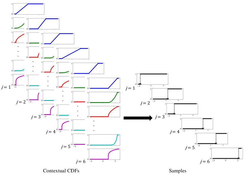
Figure 1: A visualization of the data generating process. For each $j$ with context $x^{(j)}\in\mathcal{X}$, the left column shows the $d$ contextual CDFs ($\phi_{i}(x^{(j)},\cdot),\ i\in[d]$) under the context $x^{(j)}$. For $y^{(j)}$ drawn from the CDF $F(x^{(j)},\cdot)=\theta_{*}^{\top}\Phi(x^{(j)},\cdot)$ where $\Phi(x^{(j)},\cdot):=[\phi_{i}(x^{(j)},\cdot),\dots,\phi_{d}(x^{(j)},\cdot)]^{\top}$, the right column shows the sample empirical CDF $\textup{I}_{y^{(j)}}(\cdot):=\mathbbm{1}\{y^{(j)}\leq\cdot\}$.

3 Upper bounds on estimation error

In this section, we propose an estimation paradigm for the a priori unknown parameter $\theta_{*}$ in Section 3.1, derive the upper bounds on the associated estimation error in Section 3.2, and propose a new penalized estimator that theoretically eliminates the burn-in time of the sample size in the random setting in Section 3.3.

3.1 Ridge regression estimator

We begin by formally stating our least-squares functional regression optimization problem to learn $\theta_{*}$. Given a probability measure $\mathfrak{m}$ on $S$, the sample $\{(x^{(j)},y^{(j)})\}_{j\in[n]}$, and the set of basis functions $\{\Phi_{j}\}_{j\in[n]}$, we propose to estimate $\theta_{*}$ by minimizing the (ridge or) $\ell^{2}$-regularized squared $\mathcal{L}^{2}(S,\mathfrak{m})$-distance between the estimated and empirical CDFs as follows:

$$\widehat{\theta}_{\lambda}:=\operatorname*{arg\,min}_{\theta\in\mathbb{R}^{d}}\sum_{j=1}^{n}\|\textup{I}_{y^{(j)}}-\theta^{\top}\Phi_{j}\|_{\mathcal{L}^{2}(S,\mathfrak{m})}^{2}+\lambda\|\theta\|^{2},$$ (2)

where $\lambda\geq 0$ is the hyper-parameter that determines the level of regularization, and the function observation $\textup{I}_{y^{(j)}}(t):=\mathbbm{1}\{y^{(j)}\leq t\}$ is an empirical CDF of $y^{(j)}$ that forms an unbiased estimator for $F(x^{(j)},\cdot)$ conditioned on past contexts and observations. Hence, in Scheme I, we only require that $\textup{I}_{y^{(j)}}-\theta^{\top}\Phi_{j}$ is a zero-mean function given past contexts and observations, making our analysis suitable for online learning problems where the later contexts can depend on the past contexts and observations. Notice further that $\widehat{\theta}_{\lambda}$ in (2) is an improper estimator since it may not lie in $\Delta^{d-1}$. However, since $\Delta^{d-1}$ is compact in $\mathbb{R}^{d}$, $\widetilde{\theta}_{\lambda}:=\operatorname*{arg\,min}_{\vartheta\in\Delta^{d-1}}\|\vartheta-\widehat{\theta}_{\lambda}\|_{A}$ exists for any positive definite $A\in\mathbb{R}^{d\times d}$. Moreover, since $\Delta^{d-1}$ is also convex, we have $\|\widetilde{\theta}_{\lambda}-\theta\|_{A}\leq\|\widehat{\theta}_{\lambda}-\theta\|_{A}$ (Beck, 2014, Theorem 9.9) for any $\theta\in\Delta^{d-1}$ including $\theta_{*}$. This means that an upper bound on $\|\widehat{\theta}_{\lambda}-\theta_{*}\|_{A}$ is also an upper bound on $\|\widetilde{\theta}_{\lambda}-\theta_{*}\|_{A}$. Therefore, we focus our analysis on the improper estimator $\widehat{\theta}_{\lambda}$, and note that its projection onto $\Delta^{d-1}$ yields an estimator $\widetilde{\theta}_{\lambda}$ for which the same upper bounds hold.

When $\lambda>0$, the objective function in (2) is a $(2\lambda)$-strongly convex function of $\theta\in\mathbb{R}^{d}$ (see, e.g., Bertsekas et al., 2003, for the definition), and is uniquely minimized at

$$\widehat{\theta}_{\lambda}=\left(\sum_{j=1}^{n}\int_{S}\Phi_{j}\Phi_{j}^{\top}d\mathfrak{m}+\lambda I_{d}\right)^{-1}\left(\sum_{j=1}^{n}\int_{S}\textup{I}_{y^{(j)}}\Phi_{j}d\mathfrak{m}\right).$$ (3)

For the unregularized case where $\lambda=0$, we omit the subscript $\lambda$ and write $\widehat{\theta}$ to denote a corresponding estimator in (2). Note that when $\lambda=0$, if $\mu_{\min}(\sum_{j=1}^{n}\int_{S}\Phi_{j}\Phi_{j}^{\top}d\mathfrak{m})>0$, the objective function in (2) is still strongly convex, and is uniquely minimized at $\widehat{\theta}$ given in (3) with $\lambda=0$. In practice, one can deploy standard numerical methods to compute the integral in (3), and the computational complexity of the matrix inversion is cubic in the dimension $d$. However, iterative methods can be used to obtain better dimension dependence in the running time. As a remark, since the probability density functions (PDFs) of the basis distributions may not exist, the samples in Scheme I can be dependent, and the distributions of the contexts in Scheme II are unknown, the likelihood function of the samples generally does not exist in our problem setting, which rule out the usage of maximum likelihood estimation (MLE). But our estimator (2) always exists. Moreover, we focus on non-asymptotic analysis of our estimator below and prove self-normalized upper bounds for the estimation error, which is rarely analyzed for MLEs.

Lastly, it is worth remarking upon the choice of measure $\mathfrak{m}$ used above. In order for the estimator in (2) to be well-defined, since $\textup{I}_{y}(t),\theta^{\top}\Phi(x,t)\in[0,1]$ for any $t,y\in\mathbb{R}$ and $x\in\mathcal{X}$, it suffices to ensure that $\mathfrak{m}(S)<\infty$ (i.e., $\mathfrak{m}$ is a finite measure). So, we choose to normalize the measure $\mathfrak{m}$ and set $\mathfrak{m}(S)=1$. This is the reason why we restrict $\mathfrak{m}$ to be a probability measure on $S$. Furthermore, the probability measure $\mathfrak{m}$ can in general be chosen to adapt to specific problem settings. For example, the uniform measure $\mathfrak{m}_{\mathsf{U}}$ on $S$ is often easy to compute for some choices of $S$. Specifically, if $0<\mathsf{Leb}(S)<\infty$, where $\mathsf{Leb}$ denotes the Lebesgue measure, $\mathfrak{m}_{\mathsf{U}}$ is defined by $\frac{d\mathfrak{m}_{\mathsf{U}}}{d\mathsf{Leb}}=\frac{1}{\mathsf{Leb}(S)}$, where $\frac{d\mathfrak{m}_{\mathsf{U}}}{d\mathsf{Leb}}$ is the Radon-Nikodym derivative. If $S$ is a finite set with cardinality $\#S$, $\mathfrak{m}_{\mathsf{U}}=\frac{1}{\#S}\sum_{s\in S}\delta_{s}$, where $\delta_{s}$ denotes the Dirac measure at $s$. On the other hand, when $S=\mathbb{R}$, $\mathfrak{m}$ can be set to the Gaussian measure $\gamma_{c,\sigma^{2}}$ defined by $\gamma_{c,\sigma^{2}}(dx)=\frac{1}{\sqrt{2\pi\sigma^{2}}}e^{-(x-c)^{2}/(2\sigma^{2})}dx$ with $c\in\mathbb{R}$ and $\sigma^{2}>0$.

3.2 Self-normalized bounds in various settings

When the sample is generated according to Scheme I, we prove self-normalized upper bounds on the error term $\widehat{\theta}_{\lambda}-\theta_{*}$. For any probability measure $\mathfrak{m}$ on $S$, define $U_{n}:=\sum_{j=1}^{n}\int_{S}\Phi_{j}\Phi_{j}^{\top}d\mathfrak{m}$ and $U_{n}(\lambda)=U_{n}+\lambda I_{d}$ for $n\in\mathbb{N}$ and $\lambda\geq 0$. Moreover, for $n,d\in\mathbb{N}$, $\lambda,\tau\in(0,\infty)$, and $\delta\in(0,1)$, define

$$\varepsilon_{\lambda}(n,d,\delta):=\sqrt{d\log\left(1+n/\lambda\right)+2\log(1/\delta)}+\sqrt{\lambda}\|\theta_{*}\|$$ (4)

and

$$\varepsilon(n,d,\delta,\tau):=\frac{1}{\sqrt{\tau}}\left(\sqrt{d}+\sqrt{8d\log(1/\delta)}+\frac{4}{3}\sqrt{d/n}\log(1/\delta)\right)$$ (5)

Using these definitions, the next theorem states our self-normalized upper bound on the estimation error.

Theorem 1 (Self-normalized bound in adversarial setting).

Assume $\mathfrak{m}$ is a probability measure on $S$ and $\{(x^{(j)},y^{(j)})\}_{j\in\mathbb{N}}$ is sampled according to Scheme I with $F$ defined in (1). For any $\lambda>0$ and $\delta\in(0,1)$, with probability at least $1-\delta$, the estimator defined in (2) satisfies

$$\|\widehat{\theta}_{\lambda}-\theta_{*}\|_{U_{n}(\lambda)}\leq\varepsilon_{\lambda}(n,d,\delta)$$ (6)

for all $n\in\mathbb{N}$.

Moreover, for the unregularized case, we have the following result.

Proposition 2 (Self-normalized bound in adversarial setting for unregularized estimator).

Under the same assumptions as Theorem 1, if $U_{N}$ is positive definite for some fixed $N\in\mathbb{N}$, then for any $\delta\in(0,1)$ and $n\geq N$, with probability at least $1-\delta$, the estimator defined in (2) with $\lambda=0$ satisfies

$$\|\widehat{\theta}-\theta_{*}\|_{U_{n}}\leq\varepsilon\left(n,d,\delta,\mu_{\min}(U_{n})/n\right).$$ (7)

The proofs of Theorem 1 and Proposition 2 are provided in Section 7.1. Informally, Theorem 1 and Proposition 2 convey that with high probability, the self-normalized errors $\|\widehat{\theta}_{\lambda}-\theta_{*}\|_{U_{n}(\lambda)}$ and $\|\widehat{\theta}-\theta_{*}\|_{U_{n}}$ scale as $\widetilde{O}(\sqrt{d})$ in the $\ell^{2}$-regularized and unregularized cases, where $\widetilde{O}(\cdot)$ ignores logarithmic and other sub-dominant factors. We note that Theorem 1 and Proposition 2 also imply upper bounds on the (un-normalized) error $\|\widehat{\theta}_{\lambda}-\theta_{*}\|$. Indeed, for any positive definite matrix $A\in\mathbb{R}^{d\times d}$ and vector $a\in\mathbb{R}^{d}$, we have $\|a\|\leq\mu_{\min}(A)^{-1/2}\|a\|_{A}$. Thus, for example, (6) in Theorem 1 implies that $\|\widehat{\theta}_{\lambda}-\theta_{*}\|\leq\mu_{\min}(U_{n}(\lambda))^{-1/2}\varepsilon_{\lambda}(n,d,\delta)=\widetilde{O}\big{(}\sqrt{d/(1+\mu_{\min}(U_{n}))}\big{)}$ with high probability. Then, for the projected estimator $\widetilde{\theta}_{\lambda}\in\Delta^{d-1}$, we have $\|\widetilde{\theta}_{\lambda}-\theta_{*}\|\leq\widetilde{O}\big{(}\min\{1,\sqrt{d/(1+\mu_{\min}(U_{n}))}\}\big{)}$ by the property of $\Delta^{d-1}$. When $\mu_{\min}(U_{n})=\Theta(n)$, we have $\|\widehat{\theta}_{\lambda}-\theta_{*}\|=\widetilde{O}\big{(}\sqrt{d/n}\big{)}$.

The key idea in the proof of Theorem 1 is to first notice that $\widehat{\theta}_{\lambda}-\theta_{*}=U_{n}(\lambda)^{-1}W_{n}-U_{n}(\lambda)^{-1}(\lambda\theta_{*})$, where $W_{n}:=\sum_{j=1}^{n}\int_{S}(\textup{I}_{y^{(j)}}\Phi_{j}-\theta_{*}^{\top}\Phi_{j}\Phi_{j})d\mathfrak{m}$. We next show that $\{\widebar{M}_{n}\}_{n\geq 0}$ where $\widebar{M}_{n}:=\frac{\lambda^{d/2}}{\det(U_{n}(\lambda))^{1/2}}\exp\left(\frac{1}{2}\|W_{n}\|_{U_{n}(\lambda)^{-1}}^{2}\right)$ is a super-martingale. Doob’s maximal inequality for super-martingales can then be used in conjunction with some careful algebra to establish (6).

To prove Proposition 2, we use a vector Bernstein inequality for bounded martingale difference sequences (Hsu et al., 2012a, Proposition 1.2) to show a high probability upper bound for $\|W_{n}\|$. Note that $U_{N}$ being positive definite implies that $U_{n}$ is also positive definite for any $n\geq N$. Since $\|\widehat{\theta}-\theta_{*}\|_{U_{n}}=\|W_{n}\|_{U_{n}^{-1}}\leq\|W_{n}\|/\sqrt{\mu_{\min}(U_{n})}$, we are able to establish (7).

Since the fixed design setting is a special case of the adversarial setting, Theorem 1 and Proposition 2 immediately imply the same $\widetilde{O}\big{(}\sqrt{d}\big{)}$-style upper bounds as a corollary in the fixed design setting.

Corollary 3 (Self-normalized bound in fixed design setting).

For an arbitrary probability measure $\mathfrak{m}$ on $S$ and an arbitrary sequence $\{x^{(j)}\}_{j\in\mathbb{N}}\in\mathcal{X}^{\mathbb{N}}$, assume that $y^{(j)}$ is sampled from $F(x^{(j)},\cdot)$ independently for each $j\in\mathbb{N}$ with $F$ defined in (1). For any $\lambda>0$ and $\delta\in(0,1)$, with probability at least $1-\delta$, the estimator defined in (2) satisfies (6) for all $n\in\mathbb{N}$.

If $U_{N}$ is positive definite for some fixed $N\in\mathbb{N}$, then for any $\delta\in(0,1)$ and $n\geq N$, with probability at least $1-\delta$, the estimator defined in (2) with $\lambda=0$ satisfies (7).

The proofs are the same as those of Theorem 1 and Proposition 2 and are therefore omitted.

Furthermore, based on Theorem 1 and Proposition 2, we prove self-normalized upper bounds on the estimation error when the sample is generated under Scheme II, which corresponds to the random design setting in linear regression. For convenience, for any probability measure $\mathfrak{m}$ on $S\subseteq\mathbb{R}$, define $\Sigma^{(j)}:=\mathbb{E}_{x^{(j)}\sim P_{X}^{(j)}}\left[\int_{S}\Phi_{j}\Phi_{j}^{\top}d\mathfrak{m}\right]$ and $\Sigma_{n}:=\sum_{j=1}^{n}\Sigma^{(j)}$ for $j,n\in\mathbb{N}$.

Theorem 4 (Self-normalized bound in random design setting).

Assume $\mathfrak{m}$ is a probability measure on $S$, $\{(x^{(j)},y^{(j)})\}_{j\in\mathbb{N}}$ is sampled according to Scheme II with $F$ defined in (1), and $\mu_{\min}\left(\Sigma^{(j)}\right)\geq\sigma_{\min}$ for some constant $\sigma_{\min}>0$ and all $j\in\mathbb{N}$. For any $\delta\in(0,1/2)$ and $n\geq\frac{32d^{2}}{\sigma_{\min}^{2}}\log(\frac{d}{\delta})$, with probability at least $1-2\delta$, the estimator defined in (2) with $\lambda=0$ satisfies

$$\|\widehat{\theta}-\theta_{*}\|_{\Sigma_{n}}\leq 2\varepsilon\left(n,d,\delta,\sigma_{\min}\right).$$ (8)

Moreover, for regularized estimators, we have the following result.

Proposition 5 (Self-normalized bound in random design setting for regularized estimator).

Under the same assumptions as Theorem 4, for any $\lambda>0$, $\delta\in(0,1/2)$, and $n\geq\frac{32d^{2}}{\sigma_{\min}^{2}}\log\left(\frac{d}{\delta}\right)$, with probability at least $1-2\delta$, the estimator defined in (2) satisfies

$$\|\widehat{\theta}_{\lambda}-\theta_{*}\|_{\Sigma_{n}}\leq\sqrt{2}\varepsilon_{\lambda}(n,d,\delta).$$ (9)

The proofs of Theorem 4 and Proposition 5 are given in Section 7.2. As before, they convey that in the random design setting, the self-normalized errors $\|\widehat{\theta}_{\lambda}-\theta_{*}\|_{\Sigma_{n}}$ and $\|\widehat{\theta}-\theta_{*}\|_{\Sigma_{n}}$ scale as $\widetilde{O}\big{(}\sqrt{d}\big{)}$ with high probability in the $\ell^{2}$-regularized and unregularized cases. Moreover, we once again note that Theorem 4 and Proposition 5 imply upper bounds on the (un-normalized) error $\|\widehat{\theta}_{\lambda}-\theta_{*}\|$. For example, since $\sigma_{\min}$ is a positive constant, (8) implies that $\|\widehat{\theta}-\theta_{*}\|\leq 2\mu_{\min}(\Sigma_{n})^{-1/2}\varepsilon\left(n,d,\delta,\sigma_{\min}\right)=\widetilde{O}\big{(}\sqrt{d/n}\big{)}$ with high probability since $\mu_{\min}(\Sigma_{n})\geq n\sigma_{\min}$ by Weyl’s inequality (Weyl, 1912). Moreover, it is not hard to show that for general $\Sigma_{n}$ and $\lambda>0$, (9) can be generalized to $\|\widehat{\theta}_{\lambda}-\theta_{*}\|_{\Sigma_{n}(\lambda)}=\widetilde{O}(\sqrt{d})$ which again implies that $\|\widehat{\theta}_{\lambda}-\theta_{*}\|=\widetilde{O}(\min\{1,\sqrt{d/(\mu_{\min}(\Sigma_{n})+1)}\})$.

The main idea in the proofs of Theorem 4 and Proposition 5 is to establish a high probability lower bound on $\mu_{\min}(\Delta_{n})$, where $\Delta_{n}:=\Sigma_{n}^{-\frac{1}{2}}\left(U_{n}-\Sigma_{n}\right)\Sigma_{n}^{-\frac{1}{2}}$. This can be achieved using the matrix Hoeffding’s inequality (Tropp, 2012, Theorem 1.3). Then, we show that for any $\lambda\geq 0$, $\|\widehat{\theta}_{\lambda}-\theta_{*}\|_{\Sigma_{n}}\leq(1+\mu_{\min}\left(\Delta_{n}\right))^{-1/2}\|\widehat{\theta}_{\lambda}-\theta_{*}\|_{U_{n}(\lambda)}$. For Theorem 4, we prove that $\mu_{\min}(U_{n})\geq\mu_{\min}(\Sigma_{n})(\mu_{\min}(\Delta_{n})+1)$. Then, we can lower bound $\mu_{\min}(U_{n})$ in (7) by a multiple of $\mu_{\min}(\Sigma_{n})$ with high probability. Thus, (8) follows from (7) and the high probability lower bound on $\mu_{\min}(\Delta_{n})$. For Proposition 5, (9) follows from (6) and the high probability lower bound on $\mu_{\min}(\Delta_{n})$.

We briefly compare our results in this section with related results in the literature. In the (canonical, finite dimensional) adversarial linear regression setting, Abbasi-Yadkori et al. (2011a) show an $\widetilde{O}\big{(}\sqrt{d}\big{)}$ upper bound on the self-normalized error of the (ridge or) $\ell^{2}$-regularized least-squares estimator. Our functional regression upper bound in (6) in Theorem 1 matches this scaling as shown earlier (neglecting sub-dominant factors). In the (canonical, finite dimensional) random design linear regression setting, Hsu et al. (2012b) show an $\widetilde{O}\big{(}\sqrt{d}\big{)}$ upper bound on the self-normalized error of the unregularized least-squares estimator under some conditions on the distribution of covariates. Our functional regression upper bound in (8) in Theorem 4 for the unregularized case also matches the scaling in Hsu et al. (2012b) (neglecting sub-dominant factors). Technically, following the steps in the seminal works of Abbasi-Yadkori et al. (2011a) and Hsu et al. (2012b), we conduct CDF estimation by utilizing specific properties of CDFs, which constitute some of the novel aspects in our proofs. For example, after introducing a finite measure on the support set $S$, we observe and utilize the conditional unbiasedness and boundedness of the one-sample empirical CDF $\textup{I}_{y^{(j)}}(\cdot)$ to enable us to use concentration of measure inequalities and show a generalized version of conditional sub-Gaussianity (29) for the “error term” $\int_{S}(\textup{I}_{y^{(j)}}-\theta_{*}^{\top}\Phi_{j})\Phi_{j}$. We believe that with appropriate variations of these key properties, i.e., the conditional unbiasedness and “sub-Gaussianity” mentioned above, our analysis can be generalized to other functional linear regression problems. However, due to the importance of contextual CDF estimation mentioned in Section 1, we would like the main thrust of this paper to be the specific problem of functional regression of contextual CDFs. In the context of quantile regression, Takeuchi et al. (2006) propose a nonparametric quantile estimator for a pre-specified quantile level and show that the deviation of the tail probability of their estimator from the empirical tail probability of a sample of size $n$ is $\widetilde{O}\big{(}\mathcal{R}_{n}+\sqrt{1/n}\big{)}$, where $\mathcal{R}_{n}$ denotes the Rademacher complexity of the underlying nonparametric hypothesis class for sample size $n$. As noted at the end of Section 1, although this quantile regression result appears to demonstrate a scaling of $n^{-1/2}$ similar to our results, they have a very different flavor; they hold only for one pre-specified quantile level, and one cannot be translated into the other.

Finally, we note that an upper bound on $\|\widehat{\theta}_{\lambda}-\theta_{*}\|$ immediately implies an upper bound on the KS distance between our estimated CDF and the true one. Let $\widehat{F}_{\lambda}(x,\cdot):=\widetilde{\theta}_{\lambda}^{\top}\Phi(x,\cdot)$ denote the estimated CDF for any $x\in\mathcal{X}$. Then, under the linear model (1), we have

$$\sup_{x\in\mathcal{X}}\textup{KS}(\widehat{F}_{\lambda}(x,\cdot),F(x,\cdot)) =\sup_{x\in\mathcal{X},t\in S}|(\widetilde{\theta}_{\lambda}-\theta_{*})^{\top}\Phi(x,t)|$$

$$\leq\|\widetilde{\theta}_{\lambda}-\theta_{*}\|\sup_{x\in\mathcal{X},t\in S}\|\Phi(x,t)\|$$

$$\leq\sqrt{d}\|\widehat{\theta}_{\lambda}-\theta_{*}\|,$$

where we use the Cauchy-Schwarz inequality and the fact that $\sup_{x\in\mathcal{X},t\in S}\|\Phi(x,t)\|\leq\sqrt{d}$. Since $\|\widehat{\theta}_{\lambda}-\theta_{*}\|=\widetilde{O}\big{(}\min\{1,\sqrt{d/(1+\mu_{\min}(U_{n}))}\}\big{)}$ (see discussion below Proposition 2 and 5) and $\widehat{F}_{\lambda},F\in[0,1]$, we have $\sup_{x\in\mathcal{X}}\textup{KS}(\widehat{F}_{\lambda}(x,\cdot),F(x,\cdot))\!=\!\widetilde{O}\big{(}\min\{1,d/\sqrt{(1+\mu_{\min}(U_{n}))}\}\big{)}$. It is worth mentioning that the above upper bound on the estimation error in KS distance may not be sharp because we focus on a tight analysis of the estimation of $\theta_{*}$ instead of $F(x,\cdot)$ for some $x\in\mathcal{X}$. With the knowledge of $\theta_{*}$, for any context $x$, we have a plug-in estimate of $F(x,\cdot)$, which is especially useful in the prediction phase of our learning problem since a new context corresponding to a new CDF may be given. Thus, estimating $\theta_{*}$ is a reasonable thing to do under the linear model (1). Moreover, in Appendix A, we show that when $\mu_{\min}(U_{n})=0$ ($\mu_{\min}(\Sigma_{n})=0$), the minimax risk in terms of the uniform KS distance for the estimation of $F$ (see Appendix A for the definition) is lower bounded by $\Omega(1)$ for the adversarial (random) setting. Thus, our plug-in estimate $\widehat{F}_{\lambda}$ is a reasonable estimator of $F$.

3.3 Burn-in-time-free upper bound

Note that the theoretical guarantees in Theorem 4 and Proposition 5 require a burn-in time of the sample size $n$: $n\geq\frac{32d^{2}}{\sigma_{\min}^{2}}\log(\frac{d}{\delta})$. motivated by Pires and Szepesvári (2012), we propose a new estimator $\widehat{\theta}_{\lambda}$ in (10) to eliminate the burn-in time of $n$:

$$\widecheck{\theta}_{\lambda}\in\operatorname*{arg\,min}_{\theta\in\mathbb{R}^{d}}\left(\|U_{n}(\lambda)\theta-u_{n}\|+\Delta^{U}_{n}(\delta)\|\theta\|\right),$$ (10)

where $\lambda\geq 0$, $\delta\in(0,1)$, $u_{n}:=\sum_{j=1}^{n}\int_{S}\textup{I}_{y^{(j)}}\Phi_{j}d\mathfrak{m}$, and $\Delta^{U}_{n}(\delta)$ is a positive number such that $\Delta^{U}_{n}(\delta)\geq\|U_{n}-\Sigma_{n}\|$ with probability at least $1-\delta$. For notatoinal convenience, we use $\widecheck{\theta}$ to denote $\widecheck{\theta}_{0}$. To calculate $\widecheck{\theta}_{\lambda}$ in (10), it is necessary to first choose $\Delta_{n}^{U}(\delta)$ for which we prove a lower bound in the following lemma.

Lemma 6.

Assume $\mathfrak{m}$ is a probability measure on $S$ and $\{(x^{(j)},y^{(j)})\}_{j\in\mathbb{N}}$ is sampled according to Scheme II with $F$ defined in (1). For any $\delta\in(0,1)$ and $n\in\mathbb{N}$, any $\Delta_{n}^{U}(\delta)\geq d\sqrt{8n\log(d/\delta)}$ satisfies $\Delta_{n}^{U}(\delta)\geq\Delta_{n}^{U}$ with probability at least $1-\delta$.

The proof of Lemma 6 follows from the matrix Hoeffding’s inequality (Tropp, 2012, Theorem 1.3) and the boundedness of CDFs, and is provided in Appendix B. Then, we show the following upper bound on the estimation error of $\widecheck{\theta}_{\lambda}$.

Theorem 7 (Self-normalized bound in random setting without burn-in time).

Under the same assumptions as Lemma 6, for any $\delta\in(0,1/2)$ and $n\in\mathbb{N}$, if $\mu_{\min}\left(\Sigma_{n}\right)>0$, then, with probability at least $1-2\delta$, the estimator defined in (10) with $\lambda=0$ satisfies

$$\|\widecheck{\theta}-\theta_{*}\|\leq\frac{1}{\mu_{\min}(\Sigma_{n})}\left[2d\sqrt{8n\log(d/\delta)}\|\theta_{*}\|+2\left(\sqrt{nd}+\sqrt{8nd\log(1/\delta)}+\frac{4}{3}\sqrt{d}\log(1/\delta)\right)\right].$$ (11)

The proof of Theorem 7 is provided in Section 7.3. It conveys that for any $n\in\mathbb{N}$, as long as $\mu_{(}\Sigma_{n})>0$, $\|\widecheck{\theta}-\theta_{*}\|\leq\widetilde{O}\big{(}\frac{d\sqrt{n}}{\mu_{\min}(\Sigma_{n})}\big{)}$ holds with high probability. Under the assumption that $\mu_{\min}(\Sigma^{(j)})\geq\sigma_{\min}$ for any $j\in\mathbb{N}$ as in Theorem 4 and Proposition 5, we have that $\|\widecheck{\theta}-\theta_{*}\|\leq\widetilde{O}\big{(}d/\sqrt{n}\big{)}$ with high probability for any $n\in\mathbb{N}$. Compared with the $\widetilde{O}\big{(}\sqrt{d/n}\big{)}$ upper bound of the estimation error of $\widehat{\theta}$ in Theorem 4, $\widecheck{\theta}$ suffers a larger error rate with respect to (wrt) the dimension $d$ in order to eliminate the burn-in time of the sample size $n$. Thus, $\widecheck{\theta}$ is more applicable to the estimation of $\theta_{*}$ in the regime of small sample size $n$ and small dimension $d$.

The proof of Theorem 7 builds on the upper bound shown in Pires and Szepesvári (2012) for the estimator that minimizes the unsquared penalized loss as in (10). By Pires and Szepesvári (2012, Theorem 3.4), we have that with probability at least $1-\delta$,

$$\|\Sigma_{n}(\lambda)\widecheck{\theta}_{\lambda}-\Sigma_{n}\theta_{*}\|\leq(\lambda+2\Delta^{U}_{n}(\delta))\|\theta_{*}\|+2\|u_{n}-\mathbb{E}[u_{n}]\|.$$

Then, we can bound $\|u_{n}-\mathbb{E}[u_{n}]\|$ with high probability by the vector Bernstein inequality (Hsu et al., 2012a, Proposition 1.2). By setting $\lambda=0$ and $\Delta_{n}^{U}(\delta)=d\sqrt{8n\log(d/\delta)}$ as is guaranteed by Lemma 6, we obtain (11) after some derivation.

4 Minimax lower bounds

To show that our estimator (2) is minimax optimal, we prove information theoretic lower bounds on the Euclidean norm of the estimation error for any estimator. Recall that for any distribution family $\mathcal{Q}$ and (parameter) function $\xi:\mathcal{Q}\rightarrow\mathbb{R}^{d}$, the minimax $\ell^{2}$-risk is defined as

$$\mathfrak{R}(\xi(\mathcal{Q})):=\inf_{\hat{\xi}}\sup_{Q\in\mathcal{Q}}\mathbb{E}_{z\sim Q}[\|\hat{\xi}(z)-\xi(Q)\|],$$ (12)

where the infimum is over all (possibly randomized) estimators $\hat{\xi}$ of $\xi$ based on a sample $z$, and the supremum is over all distributions in the family $\mathcal{Q}$. To specialize this definition for our problem, for any $x\in\mathcal{X}$ and $\theta\in\mathbb{R}^{d}$, let $P^{\Phi}_{Y|x;\theta}$ denote the probability measure defined by the CDF $\theta^{\top}\Phi(x,\cdot)$. Moreover, for any sequence $x^{1:n}:=(x^{(1)},\dots,x^{(n)})\in\mathcal{X}^{n}$, define the collection of product measures

$$\mathcal{P}^{d}_{x^{1:n}}:=\left\{\otimes_{j=1}^{n}P^{\Phi}_{Y|x^{(j)};\theta}:\theta\in\Delta^{d-1},\Phi\in\mathfrak{B}_{d}\right\},$$

where

$$\mathfrak{\mathcal{B}}_{d}:=\{[\phi_{1},\dots,\phi_{d}]^{\top}:\phi_{i}:\mathcal{X}\times\mathbb{R}\rightarrow[0,1]\textup{ is measurable and }\phi_{i}(x,\cdot)\textup{ is a {{CDF}} on }\mathbb{R},\forall i\in[d]\}.$$

For any distribution $P\in\mathcal{P}^{d}_{x^{1:n}}$, let $\theta(P)$ be a parameter in $\Delta^{d-1}$ such that $P=\otimes_{j=1}^{n}P^{\Phi}_{Y|x^{(j)};\theta}$. Then, we have the following theorem in the adversarial setting.

Theorem 8 (Information theoretic lower bound in adversarial setting).

For any $d\geq 2$ and any sequence $x^{1:n}\allowbreak=(x^{(1)},\dots,x^{(n)})\in\mathcal{X}^{n}$, we have

$$\mathfrak{R}(\theta(\mathcal{P}^{d}_{x^{1:n}}))=\Omega\left(\min\{1,\sqrt{d/(1+\mu_{\min}(U_{n}))}\}\right)$$ (13)

The proof uses Fano’s method (Fano, 1961) and is given in Section 8.1. Note that strictly speaking, the above theorem is written for the fixed design setting. However, a lower bound in the fixed design setting also implies the very same lower bound in adversarial setting. Furthermore, by our discussion below Theorem 1, (6) implies that in the adversarial setting,

$$\mathbb{P}\left[\|\widehat{\theta}_{\lambda}-\theta_{*}\|^{2}\geq\frac{C_{1}d\log(n)+C_{2}+C_{3}r}{1+\mu_{\min}(U_{n})}\right]\leq e^{-r}$$

for $r>0$ and some constants $C_{1}$, $C_{2}$, and $C_{3}$, which immediately implies that $\mathbb{E}[\|\widehat{\theta}_{\lambda}-\theta_{*}\|]=\widetilde{O}(\sqrt{d/(1+\mu_{\min}(U_{n}))})$ and $\mathbb{E}[\|\widetilde{\theta}_{\lambda}-\theta_{*}\|]=\widetilde{O}(\min\{1,\sqrt{d/(1+\mu_{\min}(U_{n}))}\})$. Thus, our estimator $\widetilde{\theta}_{\lambda}$ is minimax optimal. When $\mu_{\min}(U_{n})=\Theta(n)$, the optimal rate is $\widetilde{\Theta}(\sqrt{d/n})$ in the adversarial setting.

In the proof of Theorem 8, we construct a family of $\Omega(a/\sqrt{d})$-packing subsets of $\Delta^{d-1}$ for $a\in(0,1)$ under $\ell^{2}$-distance. We then show that when $\phi_{1},\dots,\phi_{d}$ are the CDFs of $d$ Bernoulli distributions, for any $\theta^{(1)}\neq\theta^{(2)}$ in such a packing subset, the Kullback-Leibler (KL) divergence (see definition in Section 8.1) satisfies

$$D(P_{Y|x^{(j)};\theta^{(1)}}\|P_{Y|x^{(j)};\theta^{(2)}})=O(a^{2}(1+\mu_{\min}(U_{n}))/d)$$

for any $j\in[n]$. Since the above family of Bernoulli distributions is a subset of $\mathcal{P}^{d}_{x^{1:n}}$, we are able to show that $\mathfrak{R}(\theta(\mathcal{P}_{x^{1:n}}))=\Omega\big{(}\sqrt{d/(1+\mu_{\min}(U_{n}))}\big{)}$ using Fano’s method and the aforementioned bound on KL divergence.

Next, to analyze minimax $\ell^{2}$-risk under the random setting, let $\mathcal{D}_{\mathcal{X}}$ denote the set of all probability distributions on $\mathcal{X}$. For any $P_{X}\in\mathcal{D}_{\mathcal{X}}$, let $P_{X}P^{\Phi}_{Y|X;\theta}$ denote the joint distribution of $(X,Y)$ such that the marginal distribution of $X$ is $P_{X}$ and the conditional distribution of $Y$ given $X=x$ is $P^{\Phi}_{Y|x;\theta}$. Define the distribution family

$$\mathcal{P}^{d}_{n}:=\big{\{}\otimes_{j=1}^{n}P_{X}^{(j)}P^{\Phi}_{Y|X;\theta}:\theta\in\mathbb{R}^{d},\ \Phi\in\mathfrak{\mathcal{B}}_{d},\ P_{X}^{(j)}\in\mathcal{D}_{\mathcal{X}}\big{\}},$$

and for any $P\in\mathcal{P}^{d}_{n}$, let $\theta(P)$ denote the parameter in $\Delta^{d-1}$ such that $P=\otimes_{j=1}^{n}P_{X}^{(j)}P^{\Phi}_{Y|X;\theta}$. Clearly, for any $x^{1:n}\in\mathcal{X}^{n}$, we have $\left\{\otimes_{j=1}^{n}\delta_{x^{(j)}}P_{Y|X;\theta}:\theta\in\Delta^{d-1}\right\}\subseteq\mathcal{P}^{d}_{n}$. Thus, each $\mathcal{P}^{d}_{x^{1:n}}$ is a collection of marginal distributions of elements belonging to such subsets of $\mathcal{P}^{d}_{n}$. Then, by the definition of minimax $\ell^{2}$-risk, Theorem 8 immediately implies the following corollary.

Corollary 9 (Information theoretic lower bound in random setting).

For any $d\geq 2$, we have

$$\mathfrak{R}(\theta(\mathcal{P}^{d}_{n}))=\Omega\left(\min\{1,\sqrt{d/(1+\mu_{\min}(\Sigma_{n}))}\}\right)$$ (14)

The detailed proof is given in Section 8.2. By our discussion below Proposition 5, our estimator $\widetilde{\theta}_{\lambda}$ ($\lambda>0$) is minimax optimal. When $\mu_{\min}(\Sigma_{n})=\Theta(n)$ as in Theorem 4 and Corollary 5, the lower bound on the Euclidean norm of the estimation error is also $\Omega\big{(}\sqrt{d/n}\big{)}$ in random setting. Again, by our discussion below Theorem 4, (8) implies that in random setting, $\mathbb{P}[\|\widehat{\theta}-\theta_{*}\|\geq C_{1}\sqrt{d/n}+C_{2}\sqrt{rd/n}+C_{3}r\sqrt{d}/n]\leq e^{-r}$ for $r>0$ and some constants $C_{1}$, $C_{2}$, and $C_{3}$, which immediately implies that $\mathbb{E}[\|\widehat{\theta}-\theta_{*}\|]=\widetilde{O}(\sqrt{d/n})$. Thus, our estimator (2) is minimax optimal with rate $\widetilde{\Theta}(\sqrt{d/n})$ in random setting when $\mu_{\min}(\Sigma_{n})=\Theta(n)$.

5 Mismatched model

In general, a mismatch may exist between the true target function and our linear model (1) with basis $\Phi$. So, in analogy with canonical linear regression where additive Gaussian random variables are used to model the error term (Montgomery et al., 2021), we consider the following mismatched model:

$$F(x,t)=\theta_{*}^{\top}\Phi(x,t)+e(x,t),\quad\forall\ x\in\mathcal{X},t\in\mathbb{R},$$ (15)

where an additive error function depending on the context is included to model the mismatch in (1). Note that in (15), each $F(x,\cdot)$ is a CDF and $e:\mathcal{X}\times S\rightarrow[-1,1]$ is a measurable function. One equivalent interpretation of (15) is as follows. Suppose that their exists another contextual CDF function $\phi_{e}$ such that $F(x,\cdot)$ is a mixture of the linear model $\theta_{*}^{\top}\Phi(x,\cdot)$ and the new feature function $\phi_{e}(x,\cdot)$, i.e., for some $q\in[0,1]$,

$$F(x,t) =(1-q)\theta_{*}^{\top}\Phi(x,t)+q\phi_{e}(x,t)=\theta_{*}^{\top}\Phi(x,t)+q\left(\phi_{e}(x,t)-\theta_{*}^{\top}\Phi(x,t)\right),\ \forall\ x\in\mathcal{X},t\in\mathbb{R}.$$

Then, we naturally obtain an additive error function $e(x,t)=q\left(\phi_{e}(x,t)-\theta_{*}^{\top}\Phi(x,t)\right)$.

Given a sample $\{(x^{(j)},y^{(j)})\}_{j\in[n]}$ generated using the mismatched model (15), let $e_{j}(t)$ denote $e(x^{(j)},t)$ for $j\in[n]$. Moreover, define $E_{n}:=\sum_{j=1}^{n}\int_{S}e_{j}\Phi_{j}d\mathfrak{m}$ and $B_{n}:=\mathbb{E}[E_{n}]=\sum_{j=1}^{n}\mathbb{E}\left[\int_{S}e_{j}\Phi_{j}d\mathfrak{m}\right]$. Then, we have the following theoretical guarantees for the task of estimating $\theta_{*}$ using the estimator in (2) in the adversarial and random settings.

Theorem 10 (Self-normalized bound in mismatched adversarial setting).

Assume $\mathfrak{m}$ is a probability measure on $S$ and $\{(x^{(j)},y^{(j)})\}_{j\in\mathbb{N}}$ is sampled according to Scheme I with $F$ defined in (15). For any $\lambda>0$ and $\delta\in(0,1)$, with probability at least $1-\delta$, the estimator defined in (2) satisfies

$$\|\widehat{\theta}_{\lambda}-\theta_{*}\|_{U_{n}(\lambda)}\leq\varepsilon_{\lambda}(n,d,\delta)+\|E_{n}\|/\sqrt{\lambda}$$ (16)

for all $n\in\mathbb{N}$.

The proof of Theorem 10 follows the same approach as the proof of Theorem 1, and it is provided in Section F.1. Furthermore, Theorem 10 directly implies a corollary for the mismatched random setting.

Corollary 11 (Self-normalized bound in mismatched random setting).

Assume $\mathfrak{m}$ is a probability measure on $S$, $\{(x^{(j)},y^{(j)})\}_{j\in\mathbb{N}}$ is sampled according to Scheme II with $F$ defined in (15), and $\mu_{\min}(\Sigma^{(j)})\geq\sigma_{\min}$ for some $\sigma_{\min}>0$ and all $j\in\mathbb{N}$. For any $\lambda>0$, $\delta\in(0,1/2)$, and $n\geq\frac{32d^{2}}{\sigma_{\min}^{2}}\log\left(\frac{d}{\delta}\right)$, with probability at least $1-2\delta$, the estimator defined in (2) satisfies

$$\|\widehat{\theta}_{\lambda}-\theta_{*}\|_{\Sigma_{n}}\leq\sqrt{2}\varepsilon_{\lambda}(n,d,\delta)+\sqrt{2/\lambda}\|B_{n}\|.$$ (17)

The proof of Corollary 11 is given in Section F.2. It follows from the proofs of Theorem 10 and Proposition 5.

In the adversarial setting, comparing (16) in Theorem 10 with (6) in Theorem 1, we see that the effect of the additive error in the mismatched model is captured by the additional $\|E_{n}\|/\sqrt{\lambda}$ term in our self-normalized error upper bound. Similarly, in the random setting, comparing (17) in Corollary 11 with (9) in Proposition 5, we again see that the effect of the additive error is captured by the additional $\sqrt{2/\lambda}\|B_{n}\|$ term in the self-normalized error upper bound.

6 Infinite dimensional model

So far, we have been assuming finite-dimensional models where the number of base contextual CDFs $\phi_{i}$’s per sample is finite. It is natural to consider generalizing the linear model to be infinite-dimensional and estimating an infinite dimensional parameter $\theta_{*}$ which shall be considered as a function on the “index” space of the base functions. In the following, we formally introduce the infinite-dimensional linear model. In Section 6.1, we present necessary definitions and technical facts for the statement of the estimator and theorem in Section 6.2, and extend the estimator $\widehat{\theta}_{\lambda}$ in (2) with properly chosen regularization and provide a high probability upper bound on the estimation error of the generalized estimator in Section 6.3.

6.1 Formal model

First, we introduce the infinite dimensional index space $\Omega$ and the generalized basis function $\Phi$. Assume that $(\Omega,\mathcal{F}_{\Omega},\mathfrak{n})$ is a measure space with $\mathfrak{n}(\Omega)<\infty$ and $\Phi:\ \mathcal{X}\times\Omega\times\mathbb{R}\rightarrow[0,1]$, $(x,\omega,t)\mapsto\Phi(x,\omega,t)$ is a $(\mathcal{B}(\mathcal{X})\otimes\mathcal{F}_{\Omega}\otimes\mathcal{B}(\mathbb{R}))/\mathcal{B}([0,1])$-measurable function (see Section 7 for the explanations of notation) such that for any $x\in\mathcal{X}$ and $\mathfrak{n}$-a.e. $\omega\in\Omega$, $\Phi(x,\omega,\cdot)$ is the CDF of some $\mathbb{R}$-valued random variable with its range contained in some Borel set $S\subseteq\mathbb{R}$.

Define the following mapping

$$\langle\cdot,\cdot\rangle:\ \mathcal{L}^{2}(\Omega,\mathfrak{n})\times\mathcal{L}^{2}(\Omega,\mathfrak{n})\rightarrow\mathbb{R},\ (f,g)\mapsto\int_{\Omega}fgd\mathfrak{n}.$$

Then, $\langle\cdot,\cdot\rangle$ is an inner product on $\mathcal{L}^{2}(\Omega,\mathfrak{n})$ and $(\mathcal{L}^{2}(\Omega,\mathfrak{n}),\langle\cdot,\cdot\rangle)$ is a Hilbert space. Let $\|\cdot\|$ denote the norm by induced $\langle\cdot,\cdot\rangle$ on $\mathcal{L}^{2}(\Omega,\mathfrak{n})$. Assume that $(\mathcal{L}^{2}(\Omega,\mathfrak{n}),\langle\cdot,\cdot\rangle)$ is separable. Then, there exists a countable orthonormal basis on $(\mathcal{L}^{2}(\Omega,\mathfrak{n}),\langle\cdot,\cdot\rangle)$. For notational convenience, we write $\mathcal{L}^{2}(\Omega,\mathfrak{n})$ to represent the Hilbert space $(\mathcal{L}^{2}(\Omega,\mathfrak{n}),\langle\cdot,\cdot\rangle)$.

Let $\boldsymbol{e}=\{e_{i}\}_{i=1}^{\infty}$ be an arbitrary fixed countable orthonormal basis of $\mathcal{L}^{2}(\Omega,\mathfrak{n})$ and $\boldsymbol{\sigma}=\{\sigma_{i}\}_{i\in\mathbb{N}}$ be an arbitrary fixed real sequence such that $\sum_{i=1}^{\infty}|\sigma_{i}|<\infty$.

Assume that there exists some unknown $\theta_{*}\in\mathcal{H}_{\boldsymbol{\sigma},\boldsymbol{e}}$ such that $\theta_{*}\geq 0$ $\mathfrak{n}$-a.e., $\int_{\Omega}\theta_{*}\mathfrak{n}=1$, and the target function $F$ satisfies the following model

$$F(x,t)=\langle\theta_{*}(\cdot),\Phi(x,\cdot,t)\rangle,\quad\forall\ x\in\mathcal{X},\ t\in\mathbb{R}.$$ (18)

6.2 Technical preliminaries

Given the sample $\{(x^{(j)},y^{(j)})\}_{j\in\mathbb{N}}\subseteq\mathcal{X}\times\mathbb{R}$, define the function $\Phi_{j}:\ \Omega\times\mathbb{R}\rightarrow[0,1],\ (\omega,t)\mapsto\Phi(x_{j},\omega,t)$ for any $j\in\mathbb{N}$. Since $\mathfrak{n}(\Omega)<\infty$ and $|\Phi(x,\omega,t)|\leq 1$ for any $x\in\mathcal{X}$, $\mathfrak{n}$-a.e. $\omega\in\Omega$, and any $t\in\mathbb{R}$, we have $\Phi_{j}\in\mathcal{L}^{2}(\Omega,\mathfrak{n})$ for any $j\in\mathbb{N}$. Then, for any $j\in\mathbb{N}$, we can define the function

$$\Psi_{j}:\mathcal{L}^{2}(\Omega,\mathfrak{n})\times S\rightarrow\mathbb{R},\ (\theta,t)\mapsto\langle\theta(\cdot),\Phi_{j}(\cdot,t)\rangle$$

Then, by Holder’s inequality, for any $j\in\mathbb{N}$ and $\theta\in\mathcal{L}^{2}(\Omega,\mathfrak{n})$, we have $\sup_{t\in\mathbb{R}}|\Psi_{j}(\theta,t)|\leq\mathfrak{n}(\Omega)\int_{\Omega}|\theta|^{2}d\mathfrak{n}<\infty$. It follows that $\Psi_{j}(\theta,\cdot)\in\mathcal{L}^{2}(S,\mathfrak{m})$. Moreover, we have that for any $n\in\mathbb{N}$, any $\theta\in\mathcal{L}^{2}(\Omega,\mathfrak{n})$, and $\mathfrak{n}$-a.e. $\omega\in\Omega$,

$$\left|\sum_{j=1}^{n}\int_{S}\Psi_{j}(\theta,t)\Phi_{j}(\omega,t)\mathfrak{m}(dt)\right|\leq \sum_{j=1}^{n}\int_{S}\left|\Psi_{j}(\theta,t)\Phi_{j}(\omega,t)\right|\mathfrak{m}(dt)$$

$$\leq n\mathfrak{n}(\Omega)\int_{\Omega}|\theta|^{2}d\mathfrak{n},$$

which, together with the fact that $\mathfrak{n}(\Omega)<\infty$ implies that the function

$$\omega\mapsto\sum_{j=1}^{n}\int_{S}\Psi_{j}(\theta,t)\Phi_{j}(\omega,t)\mathfrak{m}(dt)\in\mathcal{L}^{2}(\Omega,\mathfrak{n}).$$

Thus, for any $n\in\mathbb{N}$, we can define an operator $U_{n}:\mathcal{L}^{2}(\Omega,\mathfrak{n})\rightarrow\mathcal{L}^{2}(\Omega,\mathfrak{n})$ by

$$(U_{n}\theta)(\omega):=\sum_{j=1}^{n}\int_{S}\Psi_{j}(\theta,t)\Phi_{j}(\omega,t)\mathfrak{m}(dt)=\sum_{j=1}^{n}\int_{S}\langle\theta(\cdot),\Phi_{j}(\cdot,t)\rangle\Phi_{j}(\omega,t)\mathfrak{m}(dt)$$ (19)

for any $\theta\in\mathcal{L}^{2}(\Omega,\mathfrak{n})$. We show the following properties of $U_{n}$.

Lemma 12.

For any $n\in\mathbb{N}$, $U_{n}$ is a self-adjoint positive Hilbert-Schmidt integral operator with $\|U_{n}\|\leq n\mathfrak{n}(\Omega)$. Thus, it is also a compact operator.

The proof of Lemma 12 is provided in Appendix C.

We make the following assumption on $U_{n}$.

Assumption 13.

Assume that $e_{i}$ is an eigenfunction of $U_{n}$ with the corresponding eigenvalue denoted with $\lambda_{i}$ for any $i\in\mathbb{N}$.

Then, we can conclude from Lemma 12 that

Corollary 14.

Assume that $U_{n}$ satisfies Assumption 13 for some $n\in\mathbb{N}$. Then, we have $0\leq\lambda_{i}\leq n\mathfrak{n}(\Omega)$ for any $i\in\mathbb{N}$ and $\lambda_{i}\rightarrow 0$.

The roof of Corollary 14 is provided in Appendix C.

From now on, we assume that $U_{n}$ satisfies Assumption 13 for some $n\in\mathbb{N}$.

Define the set

$$\mathcal{L}^{2}_{\boldsymbol{\sigma}}(\Omega,\mathfrak{n}):=\left\{\theta\in\mathcal{L}^{2}(\Omega,\mathfrak{n}):\sum_{i=1}^{\infty}\frac{|\langle e_{i},\theta\rangle|^{2}}{\sigma_{i}^{4}}<\infty\right\}.$$

Then, we have that

Lemma 15.

For any $\boldsymbol{\sigma}=\{\sigma_{i}\}_{i\in\mathbb{N}}\subseteq\mathbb{R}$ such that $\sum_{i=1}^{\infty}|\sigma_{i}|<\infty$, $\mathcal{L}^{2}_{\boldsymbol{\sigma}}(\Omega,\mathfrak{n})$ is a linear subspace of $\mathcal{L}^{2}(\Omega,\mathfrak{n})$.

The proof of Lemma 15 is provided in Appendix C.

For any $\theta\in\mathcal{L}_{\boldsymbol{\sigma}}^{2}(\Omega,\mathfrak{n})$, we have

$$\sum_{i=1}^{\infty}\left|\lambda_{i}+\frac{1}{\sigma_{i}^{2}}\right|^{2}|\langle e_{i},\theta\rangle|^{2}\leq \sum_{i=1}^{\infty}2\lambda_{i}^{2}|\langle e_{i},\theta\rangle|^{2}+\sum_{i=1}^{\infty}\frac{2}{\sigma_{i}^{4}}|\langle e_{i},\theta\rangle|^{2}$$

$$\leq 2\|U_{n}\theta\|^{2}+2\sum_{i=1}^{\infty}\frac{|\langle e_{i},\theta\rangle|^{2}}{\sigma_{i}^{4}}$$

$$< \infty,$$

which implies that $\{\sum_{i=1}^{m}(\lambda_{i}+\frac{1}{\sigma_{i}^{2}})\langle e_{i},\theta\rangle e_{i}\}_{m\in\mathbb{N}}$ is a Cauchy sequence and thus converges in $\mathcal{L}^{2}(\Omega,\mathfrak{n})$ with the limit $\sum_{i=1}^{\infty}(\lambda_{i}+\frac{1}{\sigma_{i}^{2}})\langle e_{i},\theta\rangle e_{i}\in\mathcal{L}^{2}(\Omega,\mathfrak{n})$. Thus, we can define the operator $U_{n,\boldsymbol{\sigma}}:$ $\mathcal{L}_{\boldsymbol{\sigma}}^{2}(\Omega,\mathfrak{n})\rightarrow\mathcal{L}^{2}(\Omega,\mathfrak{n})$,

$$\theta\mapsto\sum_{i=1}^{\infty}\left(\lambda_{i}+\frac{1}{\sigma_{i}^{2}}\right)\langle e_{i},\theta\rangle e_{i}.$$

We show the following properties of $U_{n,\boldsymbol{\sigma}}$.

Lemma 16.

$U_{n,\boldsymbol{\sigma}}$ is bijective linear operator from $\mathcal{L}_{\boldsymbol{\sigma}}^{2}(\Omega,\mathfrak{n})$ onto $\mathcal{L}^{2}(\Omega,\mathfrak{n})$. $U_{n,\boldsymbol{\sigma}}^{-1}$ is a bounded linear operator on $\mathcal{L}^{2}(\Omega,\mathfrak{n})$ with $\|U_{n,\boldsymbol{\sigma}}^{-1}\|\leq\sup_{i\in\mathbb{N}}\sigma_{i}^{2}$ and $U_{n,\boldsymbol{\sigma}}^{-1}\theta=\sum_{i=1}^{\infty}\frac{\sigma_{i}^{2}\langle e_{i},\theta\rangle}{1+\lambda_{i}\sigma_{i}^{2}}e_{i}$ for any $\theta\in\mathcal{L}^{2}(\Omega,\mathfrak{n})$. Moreover, $U_{n,\boldsymbol{\sigma}}^{-1}$ is positive and self-adjoint.

The proof of Lemma 16 is provided in Appendix C. Consequently, we can define the following mapping

$$\|\cdot\|_{U_{n,\boldsymbol{\sigma}}}:\mathcal{L}^{2}_{\boldsymbol{\sigma}}(\Omega,\mathfrak{n})\rightarrow[0,\infty),\ \theta\mapsto\sqrt{\langle\theta,U_{n,\boldsymbol{\sigma}}\theta\rangle} =\sqrt{\sum_{i=1}^{\infty}\left(\lambda_{i}+\frac{1}{\sigma_{i}^{2}}\right)|\langle e_{i},\theta\rangle|^{2}}$$

$$=\sqrt{\|\theta\|_{U_{n}}^{2}+\sum_{i=1}^{\infty}\frac{|\langle e_{i},\theta\rangle|^{2}}{\sigma_{i}^{2}}}.$$ (20)

where $\|\theta\|_{U_{n}}:=\sqrt{\langle\theta,U_{n}\theta\rangle}$ for any $\theta\in\mathcal{L}^{2}(\Omega,\mathfrak{n})$. Define the set

$$\mathcal{H}_{\boldsymbol{\sigma},\boldsymbol{e}}:=\left\{\theta\in\mathcal{L}^{2}(\Omega):\sum_{i=1}^{\infty}\frac{|\langle e_{i},\theta\rangle|^{2}}{\sigma_{i}^{2}}<\infty\right\}$$

and the mapping

$$\langle\cdot,\cdot\rangle_{\boldsymbol{\sigma},\boldsymbol{e}}:\ \mathcal{H}_{\boldsymbol{\sigma},\boldsymbol{e}}\times\mathcal{H}_{\boldsymbol{\sigma},\boldsymbol{e}}\rightarrow\mathbb{R},\ (f,g)\mapsto\sum_{i=1}^{\infty}\frac{\langle e_{i},f\rangle\langle e_{i},g\rangle}{\sigma_{i}^{2}}.$$

Similar to the proofs of Lemma 15, we can show that $\mathcal{H}_{\boldsymbol{\sigma},\boldsymbol{e}}$ is a linear subspace of $\mathcal{L}^{2}(\Omega,\mathfrak{n})$. Moreover, $(\mathcal{H}_{\boldsymbol{\sigma},\boldsymbol{e}},\langle\cdot,\cdot\rangle_{\boldsymbol{\sigma},\boldsymbol{e}})$ is also a separable Hilbert space with $\{\sigma_{i}e_{i}\}_{i\in\mathbb{N}}$ being an orthonormal basis. For notational convenience, we write $\mathcal{H}_{\boldsymbol{\sigma},\boldsymbol{e}}$ to represent the Hilbert space $(\mathcal{H}_{\boldsymbol{\sigma},\boldsymbol{e}},\cdot,\langle\cdot\rangle_{\boldsymbol{\sigma},\boldsymbol{e}})$ and use $\|\cdot\|_{\boldsymbol{\sigma},\boldsymbol{e}}$ to denote the induced norm on $\mathcal{H}_{\boldsymbol{\sigma},\boldsymbol{e}}$. Moreover, we show the following lemma in Appendix C.

Lemma 17.

For any real sequence $\boldsymbol{\sigma}=\{\sigma_{i}\}_{i\in\mathbb{N}}$ with $\lim_{i\rightarrow\infty}\sigma_{i}=0$, we have $\mathcal{H}_{\boldsymbol{\sigma},\boldsymbol{e}}\subseteq\mathcal{L}^{2}_{\boldsymbol{\sigma}}(\Omega,\mathfrak{n})$.

6.3 Self-normalized upper bound

Since we have proved that $\Psi_{j}(\theta,\cdot)\in\mathcal{L}^{2}(S,\mathfrak{m})$ for any $j\in\mathbb{N}$ and $\theta\in\mathcal{L}^{2}(\Omega,\mathfrak{n})$, the following loss function is well-defined on $\mathcal{H}_{\boldsymbol{\sigma},\boldsymbol{e}}$,

$$L(\theta;\boldsymbol{\sigma}):=\sum_{j=1}^{n}\|\textup{I}_{y^{(j)}}(\cdot)-\Psi_{j}(\theta,t)\|^{2}_{\mathcal{L}^{2}(S,\mathfrak{m})}+\sum_{i=1}^{\infty}\frac{|\langle e_{i},\theta\rangle|^{2}}{\sigma_{i}^{2}}.$$

In fact, assuming the convention that $0/0=0$ and $1/0=\infty$, we can extend the domain of $L(\cdot;\boldsymbol{\sigma})$ to $\mathcal{L}^{2}(\Omega,\mathfrak{n})$ by extending its codomain from $[0,\infty)$ to $[0,\infty]$.

We propose to estimate $\theta_{*}$ by minimizing the above loss function over $\mathcal{H}_{\boldsymbol{\sigma},\boldsymbol{e}}$

$$\widehat{\theta}_{\boldsymbol{\sigma}}:=\operatorname*{arg\,min}_{\theta\in\mathcal{H}_{\boldsymbol{\sigma},\boldsymbol{e}}}L(\theta;\boldsymbol{\sigma}).$$ (21)

Since $\sum_{i=1}^{\infty}\frac{|\langle e_{i},\theta\rangle|^{2}}{\sigma_{i}^{2}}=\infty$ for any $\theta\in\mathcal{L}^{2}(\Omega,\mathfrak{n})$, we also have $\widehat{\theta}_{\boldsymbol{\sigma}}=\operatorname*{arg\,min}_{\theta\in\mathcal{L}^{2}(\Omega,\mathfrak{n})}L(\theta;\lambda)$. We have the following formula for $\widehat{\theta}_{\boldsymbol{\sigma}}$ in (21).

Proposition 18.

The solution to the optimization problem (21) is given as the following,

$$\widehat{\theta}_{\boldsymbol{\sigma}}=U_{n,\boldsymbol{\sigma}}^{-1}\left(\sum_{j=1}^{n}\int_{S}\textup{I}_{y^{(j)}}(t)\Phi_{j}(\cdot,t)\mathfrak{m}(dt)\right).$$ (22)

The proof of Proposition 18 is provided in Appendix D.

Under the adversarial setting, we show an upper bound for the self-normalized estimation error of $\widehat{\theta}_{\boldsymbol{\sigma}}$ in (21) in the following theorem.

Theorem 19 (Self-normalized bound in adversarial setting for infinite dimensional model).

Assume $\mathfrak{m}$ is a probability measure on $(S,\mathcal{B}(S))$, $\mathfrak{n}$ is a finite measure on $(\Omega,\mathcal{F}_{\Omega})$, $\boldsymbol{e}=\{e_{i}\}_{i=1}^{\infty}$ is an orthonormal basis of $\mathcal{L}^{2}(\Omega,\mathfrak{n})$, $\boldsymbol{\sigma}=\{\sigma_{i}\}_{i\in\mathbb{N}}$ is a real sequence such that $\sum_{i=1}^{\infty}|\sigma_{i}|<\infty$, $\theta_{*}\in\mathcal{H}_{\boldsymbol{\sigma},\boldsymbol{e}}$ satisfies $\theta_{*}\geq 0$ $\mathfrak{n}$-a.e. and $\int_{\Omega}\theta_{*}\mathfrak{n}=1$, and $\{(x^{(j)},y^{(j)})\}_{j\in\mathbb{N}}$ is sampled according to Scheme I with $F$ defined in (18).

For any given $n\in\mathbb{N}$ and any $\delta\in(0,1)$, if $U_{n}$ defined in (19) satisfies Assumption 13 and $\boldsymbol{\sigma}$ satisfies that $|\sigma_{i}|<\frac{1}{\sqrt{\lambda_{i}}}$ for any $i\in\mathbb{N}$, then, with probability at least $1-\delta$, the estimator $\widehat{\theta}_{\boldsymbol{\sigma}}$ defined in (21) satisfies

$$\|\widehat{\theta}_{\boldsymbol{\sigma}}-\theta_{*}\|_{U_{n,\boldsymbol{\sigma}}}\leq\sqrt{\left(\sum_{i=1}^{\infty}\log\left(1+\lambda_{i}\sigma_{i}^{2}\right)\right)+2\log\frac{1}{\delta}}+\|\theta_{*}\|_{\boldsymbol{\sigma},\boldsymbol{e}}.$$ (23)

In particular, for any given $n\in\mathbb{N}$ and any $\delta\in(0,1)$, if $U_{n}$ defined in (19) satisfies Assumption 13 and $\boldsymbol{\sigma}$ satisfies that $|\sigma_{i}|<\frac{1}{\sqrt{n\mathfrak{n}(\Omega)}}$ for any $i\in\mathbb{N}$, then, with probability at least $1-\delta$, the estimator $\widehat{\theta}_{\boldsymbol{\sigma}}$ defined in (21) satisfies

$$\|\widehat{\theta}_{\boldsymbol{\sigma}}-\theta_{*}\|_{U_{n,\boldsymbol{\sigma}}}\leq\sqrt{\left(\sum_{i=1}^{\infty}\log\left(1+n\mathfrak{n}(\Omega)\sigma_{i}^{2}\right)\right)+2\log\frac{1}{\delta}}+\|\theta_{*}\|_{\boldsymbol{\sigma},\boldsymbol{e}}.$$ (24)

The detailed proof of Theorem 19 is provided in Section 9. Since $\sum_{i=1}^{\infty}|\sigma_{i}|<\infty$ and $\theta_{*}\in\mathcal{H}_{\boldsymbol{\sigma},\boldsymbol{e}}$, we have that $\|\theta_{*}\|_{\boldsymbol{\sigma},\boldsymbol{e}}<\infty$ and $\sum_{i=1}^{\infty}|\sigma_{i}|^{2}<\infty$ which implies that

$$\sum_{i=1}^{\infty}\log\left(1+\lambda_{i}\sigma_{i}^{2}\right)\leq\sum_{i=1}^{\infty}\log\left(1+n\mathfrak{n}(\Omega)\sigma_{i}^{2}\right)<\infty.$$

Thus, the RHS terms in (23) and (24) are finite and $\widehat{\theta}_{\boldsymbol{\sigma}}-\theta_{*}\in\mathcal{L}^{2}_{\boldsymbol{\sigma}}(\Omega,\mathfrak{n})$. (24) conveys that with high probability,

$$\|\widehat{\theta}_{\boldsymbol{\sigma}}-\theta_{*}\|_{U_{n,\boldsymbol{\sigma}}}\leq\widetilde{O}\left(1+\sqrt{\sum_{i=1}^{\infty}\log(1+n\mathfrak{n}(\Omega)\sigma_{i}^{2})}\right).$$

When $\Omega=[d]$ for some $d\in\mathbb{N}$ and $\mathfrak{n}$ is the counting measure on $\Omega$, (21) reduces to (2) after setting $e_{i}=\mathbbm{1}_{\{i\}}$ and $\sigma_{i}=\frac{1}{\sqrt{\lambda}}$ for any $i\in[d]$ and some $\lambda>0$. Then, by (20) and (24), we have $\|\widehat{\theta}_{\boldsymbol{\sigma}}-\theta_{*}\|_{U_{n}}\leq\widetilde{O}\big{(}\sqrt{d}\big{)}$ and

$$\|\widehat{\theta}_{\boldsymbol{\sigma}}-\theta_{*}\|_{U_{n}}\leq\widetilde{O}\big{(}\sqrt{d/(1+\mu_{\min}(U_{n}))}\big{)},$$

which also recovers the result in Theorem 1. Thus, Theorem 19 is a generalization of Theorem 1 for the possibly infinite dimensional model (18).

The proof of Theorem 19 also generalizes the approach used in the proof of Theorem 1 to the setting of the infinite dimensional model (18). However, there are plenty of technical challenges in dealing with the infinite dimensional $\mathcal{L}^{2}$ space. First of all, since the vectors in the proof of Theorem 1 are generalized to functions and the matrices are generalized to operators, we need to ensure that these functions are well-defined in some proper spaces and figure out the domain/codomain and properties (e.g., linearity, boundedness, self-adjointness, positivity, compactness, invertibility, etc) of those operators. As in the proof of Theorem 1, we would like to write $\widehat{\theta}_{\boldsymbol{\sigma}}-\theta_{*}=U_{n,\boldsymbol{\sigma}}^{-1}W_{n}-U_{n,\boldsymbol{\sigma}}^{-1}(\varsigma\theta_{*})$ where,

$$W_{n}:=\sum_{j=1}^{n}\int_{S}\textup{I}_{y^{(j)}}(t)\Phi_{j}(\omega,t)\mathfrak{m}(dt)-\int_{S}\Psi_{j}(\theta_{*},t)\Phi_{j}(\omega,t)\mathfrak{m}(dt),$$

and $\varsigma\theta_{*}:=\sum_{i=1}^{\infty}\frac{\langle e_{i},\theta_{*}\rangle}{\sigma_{i}^{2}}e_{i}$. However, this sequence $\{\sum_{i=1}^{m}\frac{\langle e_{i},\theta_{*}\rangle}{\sigma_{i}^{2}}e_{i}\}_{m\in\mathbb{N}}$ only converges for $\theta_{*}\in\mathcal{L}^{2}_{\boldsymbol{\sigma}}(\Omega,\mathfrak{n})$ but not $\mathcal{H}_{\boldsymbol{\sigma},\boldsymbol{e}}$. Thus, for general $\theta_{*}\in\mathcal{H}_{\boldsymbol{\sigma},\boldsymbol{e}}$, $\varsigma\theta_{*}$ does not exist and we instead consider the finite-rank operator

$$\varsigma_{m}:\theta\mapsto\sum_{i=1}^{m}\frac{\langle e_{i},\theta\rangle}{\sigma_{i}^{2}}e_{i}$$

on $\mathcal{L}^{2}(\Omega,\mathfrak{n})$ and the sequence $\{\theta_{*,m}:=U_{n,\boldsymbol{\sigma}}^{-1}(U_{n}\theta_{*}+\varsigma_{m}\theta_{*})\}_{m\in\mathbb{N}}$ which we show satisfies $\|\theta_{*,m}-\theta_{*}\|_{U_{n,\boldsymbol{\sigma}}}\rightarrow 0$ as $m\rightarrow\infty$. Then, since it suffices to bound

$$\|\widehat{\theta}_{\boldsymbol{\sigma}}-\theta_{*,m}\|_{U_{n,\boldsymbol{\sigma}}}\leq\|U_{n,\boldsymbol{\sigma}}^{-1}W_{n}\|_{U_{n,\boldsymbol{\sigma}}}+\|U_{n,\boldsymbol{\sigma}}^{-1}\varsigma_{m}\theta_{*}\|_{U_{n,\boldsymbol{\sigma}}}\leq\|W_{n}\|_{U_{n,\boldsymbol{\sigma}}^{-1}}+\|\theta_{*}\|_{\boldsymbol{\sigma},\boldsymbol{e}}.$$

To bound $\|W_{n}\|_{U_{n,\boldsymbol{\sigma}}^{-1}}$, we use the martingale approach as in the proof of Theorem 1. However, after proving that

$$\Big{\{}M_{n}(\alpha):=\exp\big{(}\langle\alpha,W_{n}\rangle-\frac{1}{2}\|\alpha\|^{2}_{U_{n}}\big{)}\Big{\}}_{n\geq 0}$$

is a super-martingale for any $\alpha\in\mathcal{L}^{2}(\Omega,\mathfrak{n})$ wrt the natural filtration

$$\{\mathcal{F}_{n}:=\sigma(x_{1},y_{1},\dots,x_{n},y_{n},x_{n+1})\}_{n\geq 0},$$

it is difficult to pick a properly defined “Gaussian” random variable in $\mathcal{L}^{2}(\Omega,\mathfrak{n})$. Inspired by Lifshits (2012, Example 2.2), we define $\beta=\sum_{i=1}^{\infty}\sigma_{i}\zeta_{i}e_{i}$ with $\{\zeta_{i}\}_{i\in\mathbb{N}}$ being a sequence of independent $N(0,1)$-random variables. Note that $\beta\in\mathcal{L}^{2}(\Omega,\mathfrak{n})$ a.s. if $\sum_{i=1}^{\infty}\sigma_{i}^{2}<\infty$. Thus, we can define $\widebar{M}_{n}:=\mathbb{E}[M_{n}(\beta)|\mathcal{F}_{\infty}]$ with $\mathcal{F}_{\infty}:=\sigma(\cup_{n=1}^{\infty}\mathcal{F}_{n})$. Then, we prove that $\{M_{n}\}_{n\geq 0}$ is also a super-martingale wrt $\{\mathcal{F}_{n}\}_{n\geq 0}$ and the question remained is to calculate $M_{n}$. However, directly generalizing (34), we would get

$$``\|W_{n}\|^{2}_{U_{n,\boldsymbol{\sigma}}^{-1}}-\|\beta-U_{n,\boldsymbol{\sigma}}^{-1}W_{n}\|^{2}_{U_{n,\boldsymbol{\sigma}}}=2\langle\beta,W_{n}\rangle-\|\beta\|^{2}_{U_{n,\boldsymbol{\sigma}}}"$$

which does not make sense because $\|\beta\|_{U_{n,\boldsymbol{\sigma}}}$ could be $\infty$ with positive probability. Since it is hard to deal with this in the integration over the the law of $\beta$, we instead adopt the similar approach as we do for $\theta_{*}$. Define $\beta_{m}:=\sum_{i=1}^{m}\sigma_{i}\zeta_{i}e_{i}$ and $W_{n,m}:=\sum_{i=1}^{m}\langle e_{i},W_{n}\rangle e_{i}$. Then, after some calculation, we get

$$\|W_{n,m}\|^{2}_{U_{n,\boldsymbol{\sigma}}^{-1}}-\|\beta_{m}-U_{n,\boldsymbol{\sigma}}^{-1}W_{n,m}\|^{2}_{U_{n,\boldsymbol{\sigma}}}=2\langle\beta_{m},W_{n,m}\rangle-\|\beta_{m}\|^{2}_{U_{n,\boldsymbol{\sigma}}}$$

and

$$\mathbb{E}[\exp(H_{m})|\mathcal{F}_{\infty}]=\frac{1}{\sqrt{\prod_{i=1}^{m}(1+\lambda_{i}\sigma_{i}^{2})}}\exp\left(\frac{1}{2}\|W_{n,m}\|^{2}_{U_{n,\boldsymbol{\sigma}}^{-1}}\right),$$

where $\exp(H_{m}):=\exp\left\{\langle\beta_{m},W_{n,m}\rangle-\frac{1}{2}\|\beta_{m}\|^{2}_{U_{n}}\right\}$. Afterwards, we use dominated convergence theorem to conclude that,

$$\lim_{m\rightarrow\infty}\mathbb{E}[\exp(H_{m})|\mathcal{F}_{\infty}]=\mathbb{E}[M_{n}|\mathcal{F}_{\infty}]=\widebar{M}_{n},\ a.s..$$

The verification the integrability of the dominating function

$$\exp\Big{(}n\sum_{i=1}^{\infty}|\sigma_{i}\zeta_{i}|+\frac{1}{2}\sum_{i=1}^{\infty}\lambda_{i}\sigma_{i}^{2}\zeta_{i}^{2}\Big{)}$$

is also quite technical, during which the condition that $\sum_{i=1}^{\infty}|\sigma_{i}|<\infty$ is used. Finally, we obtain that

$$\widebar{M}_{n}=\frac{1}{\sqrt{\prod_{i=1}^{\infty}(1+\lambda_{i}\sigma_{i}^{2})}}\exp\left(\frac{1}{2}\|W_{n}\|^{2}_{U_{n,\boldsymbol{\sigma}}^{-1}}\right).$$

Then, by applying Doob’s maximal inequality for super-martingales, we can bound $\|W_{n}\|^{2}_{U_{n,\boldsymbol{\sigma}}^{-1}}$ which yields the final bound on $\|\widehat{\theta}_{\boldsymbol{\sigma}}-\theta_{*}\|_{U_{n,\boldsymbol{\sigma}}}$ in (23). (24) immediately follows from (23) and Corollary 14.

7 Proofs of upper bounds for the finite dimensional model

We first briefly expand on the notation for the proofs of our theoretical results. For any topological space $A$, let $\mathcal{B}(A)$ denote the Borel $\sigma$-algebra of $A$. For any two measurable spaces, $(A_{1},\mathcal{A}_{1})$ and $(A_{2},\mathcal{A}_{2})$, a function $f:A_{1}\rightarrow A_{2}$ is $\mathcal{A}_{1}/\mathcal{A}_{2}$-measurable if for any $E\in\mathcal{A}_{2}$, we have $f^{-1}(E)\in\mathcal{A}_{1}$. When $\mathcal{A}_{2}$ is the Borel $\sigma$-algebra on $A_{2}$, we sometimes write $f$ is $\mathcal{A}_{1}$-measurable to mean that $f$ is $\mathcal{A}_{1}/\mathcal{A}_{2}$-measurable for brevity. When $\mathcal{A}_{1}$ is the Borel $\sigma$-algebra on $A_{1}$ and $\mathcal{A}_{2}$ is the Borel $\sigma$-algebra on $A_{2}$, we sometimes simply write $f$ is measurable to mean that $f$ is $\mathcal{A}_{1}/\mathcal{A}_{2}$-measurable for brevity. For any two $\sigma$-finite measure spaces $(A_{1},\mathcal{A}_{1},\nu_{1})$ and $(A_{2},\mathcal{A}_{2},\nu_{2})$, let $A_{1}\times A_{1}:=\{(a_{1},a_{2}):a_{1}\in A_{1},a_{2}\in A_{2}\}$ denote the product space, let $\mathcal{A}_{1}\otimes\mathcal{A}_{2}:=\sigma(\{E_{1}\times E_{2}:E_{1}\in\mathcal{A}_{1},E_{2}\in\mathcal{A}_{2}\})$ denote the product $\sigma$-algebra of $\mathcal{A}_{1}$ and $\mathcal{A}_{2}$ on $A_{1}\times A_{2}$, and let $\nu_{1}\otimes\nu_{2}$ denote the product measure of $\nu_{1}$ and $\nu_{2}$ on $(A_{1}\times A_{2},\mathcal{A}_{1}\otimes\mathcal{A}_{2})$ (i.e., $\nu_{1}\otimes\nu_{2}(E_{1}\times E_{2})=\nu_{1}(E_{1})\nu_{2}(E_{2})$ for any $E_{1}\in\mathcal{A}_{1}$ and $E_{2}\in\mathcal{A}_{2}$) whose existence is guaranteed by Carathéodory’s extension theorem. Then, $(A_{1}\times A_{2},\mathcal{A}_{1}\otimes\mathcal{A}_{2},\nu_{1}\otimes\nu_{2})$ is the product measure space of $(A_{1},\mathcal{A}_{1},\nu_{1})$ and $(A_{2},\mathcal{A}_{2},\nu_{2})$. When $A_{1}=A_{2}$ and $\mathcal{A}_{1}=\mathcal{A}_{2}$, we will write $\mathcal{A}_{1}^{2}$ to represent $\mathcal{A}_{1}\otimes\mathcal{A}_{1}$. When $A_{1}=A_{2}$, $\mathcal{A}_{1}=\mathcal{A}_{2}$, and $\nu_{1}=\nu_{2}$, we will write $\nu_{1}^{2}$ to represent $\nu_{1}\otimes\nu_{1}$.

Note that according to our assumptions, $\mathcal{X}$ is a Polish space equipped with the Borel $\sigma$-algebra $\mathcal{B}(\mathcal{X})$, $\phi_{i}:\mathcal{X}\times S\rightarrow[0,1]$ is $(\mathcal{B}(\mathcal{X})\otimes\mathcal{B}(S))/\mathcal{B}([0,1])$-measurable for each $i\in[d]$, and $e:\mathcal{X}\times S\rightarrow[-1,1]$ is $(\mathcal{B}(\mathcal{X})\otimes\mathcal{B}(S))/\mathcal{B}([-1,1])$-measurable.

In the proofs of the main results, we consider an arbitrary probability measure $\mathfrak{m}$ on $(S,\mathcal{B}(S))$. Since there is no ambiguity, for brevity, we omit “$d\mathfrak{m}$” in the notation for integrals. Note that some quantities defined below depend on the chosen probability measure $\mathfrak{m}$.

7.1 Proofs of Theorem 1 and Proposition 2

In the proofs of Theorem 1 (Section 7.1.1) and Proposition 2 (Section 7.1.2), we use the following measure-theoretic treatment of probability spaces. (The notation we use can be found at the beginning of Section 7.) The underlying probability space for the sample $\{(x^{(j)},y^{(j)})\}_{j\in\mathbb{N}}$ is $([0,1]^{\mathbb{N}},\mathcal{B}([0,1])^{\mathbb{N}},\mathbb{P})$, where $[0,1]^{\mathbb{N}}=\{(\xi^{(1)},\xi^{(2)},\dots):\xi^{(j)}\in[0,1]\}$, and,

$$\mathcal{B}([0,1])^{\mathbb{N}}:=\sigma(\{B_{1}\times\cdots\times B_{n}:B_{1},\dots,B_{n}\in\mathcal{B}([0,1]),n\in\mathbb{N}\})$$

is the $\sigma$-algebra generated by all finite products of Borel sets on $[0,1]$, and $\mathbb{P}|_{[0,1]^{n}}=\mathsf{Leb}^{n}=\otimes_{j=1}^{n}\mathsf{Leb}$ with $\mathsf{Leb}$ being the Lebesgue measure on $([0,1],\mathcal{B}([0,1]))$. The existence of the above probability space is guaranteed by Kolmogorov’s extension theorem. Define the random vector $\Xi=(\Xi^{(j)})_{j\in\mathbb{N}}$ on $([0,1]^{\mathbb{N}},\mathcal{B}([0,1])^{\mathbb{N}})$ to be the identity mapping, i.e., $\Xi:[0,1]^{\mathbb{N}}\rightarrow[0,1]^{\mathbb{N}}$, $(\xi^{(j)})_{j\in\mathbb{N}}\mapsto(\xi^{(j)})_{j\in\mathbb{N}}$. Then, $\mathbb{P}$ is also the probability measure on $([0,1]^{\mathbb{N}},\mathcal{B}([0,1]^{\mathbb{N}}))$ induced by $\Xi$, and $\Xi$ follows the uniform distribution on $[0,1]^{\mathbb{N}}$. Suppose $\{(x^{(j)},y^{(j)})\}_{j\in\mathbb{N}}$ is sampled according to Scheme I with $F$ defined in (1). Then, according to Bogachev (2007, Proposition 10.7.6), for each $j\in\mathbb{N}$, there exist some $(\mathcal{B}(\mathcal{X})\otimes\mathcal{B}(S))^{j-1}\otimes\mathcal{B}([0,1])/\mathcal{B}(\mathcal{X})$-measurable function,

$$h_{X}^{(j)}:\ (\mathcal{X}\times S)^{j-1}\times[0,1]\rightarrow\mathcal{X},$$

and $(\mathcal{B}(\mathcal{X})\otimes\mathcal{B}(S))^{j-1}\otimes\mathcal{B}(\mathcal{X})\otimes\mathcal{B}([0,1])/\mathcal{B}(S)$-measurable function

$$h_{Y}^{(j)}:\ (\mathcal{X}\times S)^{j-1}\times\mathcal{X}\times[0,1]\rightarrow S$$

such that

$$x^{(j)} =h_{X}^{(j)}(x^{(1)},y^{(1)},\dots,x^{(j-1)},y^{(j-1)},\Xi^{(2j-1)}),$$

$$y^{(j)} =h_{Y}^{(j)}(x^{(1)},y^{(1)},\dots,x^{(j-1)},y^{(j-1)},x^{(j)},\Xi^{(2j)}),$$

and,

$$\mathbb{E}\left[\mathbbm{1}\left\{h_{Y}^{(j)}(x^{(1)},y^{(1)},\dots,x^{(j-1)},y^{(j-1)},x^{(j)},\Xi^{(2j)})\leq t\right\}\big{|}\mathcal{F}_{j-1}\right]=\theta_{*}^{\top}\Phi(x^{(j)},t)$$ (25)

for any $t\in S$ and $j\in\mathbb{N}$, where $\mathcal{F}_{j}:=\sigma\left(\big{\{}\Xi^{(k)}:k\in[2j+1]\big{\}}\right)$ is the sub $\sigma$-algebra of $\mathcal{B}([0,1])^{\mathbb{N}}$ generated by the random variables $\Xi^{(1)},\dots,\Xi^{(2j+1)}$. By definition, we have that $y^{(j)}$ is $\mathcal{F}_{j}/\mathcal{B}(S)$-measurable for each $j\in\mathbb{N}$ and $\{\mathcal{F}_{j}\}_{j=0}^{\infty}$ forms a filtration of $([0,1]^{\mathbb{N}},\mathcal{B}([0,1])^{\mathbb{N}},\mathbb{P})$. Therefore, $\left\{y^{(j)}\right\}_{j\in\mathbb{N}}$ is $\left\{\mathcal{F}_{j}\right\}_{j\in\mathbb{N}}$-adapted.

By the above construction, for each $j\in\mathbb{N}$, $x^{(j)}:\ [0,1]^{\mathbb{N}}\rightarrow\mathcal{X}$, $\xi\mapsto x^{(j)}(\xi)$ is a $\mathcal{F}_{j-1}/\mathcal{B}(\mathcal{X})$-measurable function. Thus, for each $j\in\mathbb{N}$, the function $\widetilde{h}_{X}:$ $[0,1]^{\mathbb{N}}\times S\rightarrow\mathcal{X}\times S$, $(\xi,t)\mapsto(x^{(j)}(\xi),t)$ is $(\mathcal{F}_{j-1}\otimes\mathcal{B}(S))/(\mathcal{B}(\mathcal{X})\otimes\mathcal{B}(S))$-measurable. Since $\phi_{i}:$ $\mathcal{X}\times S\rightarrow[0,1]$, $(x,t)\mapsto\phi_{i}(x,t)$ is $\mathcal{B}(\mathcal{X})\otimes\mathcal{B}(S)/\mathcal{B}([0,1])$-measurable, we know that $\widetilde{\phi}_{i}^{(j)}:$ $[0,1]^{\mathbb{N}}\times S\rightarrow[0,1]$, $(\xi,t)\mapsto\phi_{i}(x^{(j)}(\xi),t)$ is $(\mathcal{F}_{j-1}\otimes\mathcal{B}(S))/\mathcal{B}([0,1])$-measurable. Therefore, the vector-valued function $\Phi_{j}:$ $[0,1]^{\mathbb{N}}\times S\rightarrow[0,1]^{d}$, $(\xi,t)\mapsto[\phi_{1}(x^{(j)}(\xi),t),\dots,\phi_{d}(x^{(j)}(\xi),t)]=[\widetilde{\phi}_{1}^{(j)}(\xi,t),\dots,\widetilde{\phi}_{d}^{(j)}(\xi,t)]$ is $(\mathcal{F}_{j-1}\otimes\mathcal{B}(S))/\mathcal{B}([0,1]^{d})$-measurable for each $j\in\mathbb{N}$.

7.1.1 Proof of Theorem 1

Proof.

Define $V_{j}:=\int_{S}\textup{I}_{y^{(j)}}\Phi_{j}-\int_{S}\theta_{*}^{\top}\Phi_{j}\Phi_{j}$. Since we have proved above that for each $j\in\mathbb{N}$, $y^{(j)}$ is $\mathcal{F}_{j}$-measurable and the function $S\times S\ni(y,t)\mapsto\mathbbm{1}\{y\leq t\}\in[0,1]$ is $\mathcal{B}(S)^{2}$-measurable, we have that $\textup{I}_{y^{(j)}}:$ $[0,1]^{\mathbb{N}}\times S\rightarrow[0,1]$, $\textup{I}_{y^{(j)}}(\xi,t)=\mathbbm{1}\{y^{(j)}(\xi)\leq t\}$ is $\mathcal{F}_{j}\otimes\mathcal{B}(S)$-measurable. Since we have also proved above that for each $j\in\mathbb{N}$, $\Phi_{j}$ is $\mathcal{F}_{j-1}\otimes\mathcal{B}(S)$-measurable, by Fubini’s theorem and (25), we have that $\int_{S}\theta_{*}^{\top}\Phi_{j}\Phi_{j}$ is $\mathcal{F}_{j-1}$-measurable, $V_{j}$ is $\mathcal{F}_{j}$-measurable, and

$$\mathbb{E}[V_{j}|\mathcal{F}_{j-1}]= \mathbb{E}\left[\int_{S}\textup{I}_{y^{(j)}}\Phi_{j}\big{|}\mathcal{F}_{j-1}\right]-\int_{S}\theta_{*}^{\top}\Phi_{j}\Phi_{j}$$

$$= \int_{S}\mathbb{E}\left[\textup{I}_{y^{(j)}}\big{|}\mathcal{F}_{j-1}\right]\Phi_{j}-\int_{S}\theta_{*}^{\top}\Phi_{j}\Phi_{j}$$

$$= \int_{S}\theta_{*}^{\top}\Phi_{j}\Phi_{j}-\int_{S}\theta_{*}^{\top}\Phi_{j}\Phi_{j}$$

$$= 0.$$ (26)

For any $\alpha\in\mathbb{R}^{d}$, define $M_{0}(\alpha)=1$. Then, $M_{0}(\alpha)$ is $\mathcal{F}_{0}$-measurable for any $\alpha\in\mathbb{R}^{d}$. For $n\in\mathbb{N}$, define $M_{n}(\alpha):=\exp\left\{\alpha^{\top}W_{n}-\frac{1}{2}\|\alpha\|^{2}_{U_{n}}\right\}$ with $W_{n}:=\sum_{j=1}^{n}V_{j}$ and $U_{n}=\sum_{j=1}^{n}\int_{S}\Phi_{j}\Phi_{j}^{\top}$. Since $\Phi_{j}$ is $\mathcal{F}_{j-1}\otimes\mathcal{B}(S)$-measurable and $V_{j}$ is $\mathcal{F}_{j}$-measurable, by Fubini’s theorem, $U_{n}$ is $\mathcal{F}_{n-1}$-measurable and $W_{n}$ is $\mathcal{F}_{n}$-measurable for each $n\in\mathbb{N}$. Thus, $M_{n}(\alpha)$ is also $\mathcal{F}_{n}$-measurable for any $\alpha\in\mathbb{R}^{d}$ and $n\in\mathbb{N}$. Moreover, note that the function $\mathbb{R}^{d}\times\mathbb{R}^{d}\times\mathbb{R}^{d\times d}\rightarrow(0,\infty)$, $(\alpha,W,U)\mapsto\exp\left\{\alpha^{\top}W-\frac{1}{2}\|\alpha\|^{2}_{U}\right\}$ is measurable. Hence, $M_{n}:$ $[0,1]^{\mathbb{N}}\times\mathbb{R}^{d}\rightarrow(0,\infty)$, $(\xi,\alpha)\mapsto\exp\big{\{}\alpha^{\top}W_{n}(\xi)-\frac{1}{2}\|\alpha\|^{2}_{U_{n}(\xi)}\big{\}}$ is $\mathcal{F}_{n}\otimes\mathcal{B}(\mathbb{R}^{d})$-measurable. Thus, for any $\alpha\in\mathbb{R}^{d}$, $\{M_{n}(\alpha)\}_{n\geq 0}$ is $\{\mathcal{F}_{n}\}_{n\geq 0}$-adapted. Besides, for any $\alpha\in\mathbb{R}^{d}$ and $n\in\mathbb{N}$, we have

$$\mathbb{E}[M_{n}(\alpha)|\mathcal{F}_{n-1}]= M_{n-1}(\alpha)\mathbb{E}\left[\exp\left\{\alpha^{\top}V_{n}-\frac{1}{2}\alpha^{\top}\left(\int_{S}\Phi_{n}\Phi_{n}^{\top}\right)\alpha\right\}\middle|\mathcal{F}_{n-1}\right]$$

$$= M_{n-1}(\alpha)\frac{\mathbb{E}\left[\exp\left\{\alpha^{\top}V_{n}\right\}|\mathcal{F}_{n-1}\right]}{\exp\left\{\frac{1}{2}\int_{S}\left(\alpha^{\top}\Phi_{n}\right)^{2}\right\}}.$$ (27)

Since $-\int_{S}|\alpha^{\top}\Phi_{n}|\leq\alpha^{\top}V_{n}\leq\int_{S}|\alpha^{\top}\Phi_{n}|$ almost surely (a.s.), we have

$$\mathbb{E}\left[\exp\left\{\alpha^{\top}V_{n}\right\}|\mathcal{F}_{n-1}\right] \leq\exp\left\{\frac{4}{8}\left(\int_{S}|\alpha^{\top}\Phi_{n}|\right)^{2}\right\}$$ (28)

$$\leq\exp\left\{\frac{1}{2}\int_{S}\left(\alpha^{\top}\Phi_{n}\right)^{2}\right\},$$ (29)

where (28) follows from Hoeffding’s lemma (Hoeffding, 1963), and (29) follows from the Cauchy-Schwarz inequality and the fact that $\int_{S}1=\mathfrak{m}(S)=1$. Then, by (27) and (29), we have

$$\mathbb{E}[M_{n}(\alpha)|\mathcal{F}_{n-1}]\leq M_{n-1}(\alpha)\frac{\exp\left\{\frac{1}{2}\int_{S}\left(\alpha^{\top}\Phi_{n}\right)^{2}\right\}}{\exp\left\{\frac{1}{2}\int_{S}\left(\alpha^{\top}\Phi_{n}\right)^{2}\right\}}=M_{n-1}(\alpha).$$ (30)

Since $M_{0}(\alpha)=1$ and $M_{n}(\alpha)\geq 0$, for any $\alpha\in\mathbb{R}^{d}$, $\{M_{n}(\alpha)\}_{n\geq 0}$ is a super-martingale.

Now for any $n\geq 0$, define $\widebar{M}_{n}:=\int_{\mathbb{R}^{d}}M_{n}(\alpha)h(\alpha)d\alpha$, with $d\alpha$ denoting $\mathsf{Leb}(d\alpha)$ where the Lebesgue measure is on $(\mathbb{R}^{d},\mathcal{B}(\mathbb{R}^{d}))$ and

$$h(\alpha)=\left(\frac{\lambda}{2\pi}\right)^{\frac{d}{2}}\exp\left\{-\frac{\lambda}{2}\alpha^{\top}\alpha\right\}=\left(\frac{\lambda}{2\pi}\right)^{\frac{d}{2}}\exp\left\{-\frac{1}{2}\|\alpha\|^{2}_{\lambda I_{d}}\right\}.$$ (31)

Recall that $U_{n}(\lambda)=U_{n}+\lambda I_{d}$. Then, for $n\geq 1$, we have

$$\widebar{M}_{n}= \left(\frac{\lambda}{2\pi}\right)^{\frac{d}{2}}\int_{\mathbb{R}^{d}}\exp\left\{\alpha^{\top}W_{n}-\frac{1}{2}\|\alpha\|^{2}_{U_{n}}-\frac{1}{2}\|\alpha\|^{2}_{\lambda I_{d}}\right\}d\alpha$$

$$= \left(\frac{\lambda}{2\pi}\right)^{\frac{d}{2}}\int_{\mathbb{R}^{d}}\exp\left\{\frac{1}{2}\|W_{n}\|_{U_{n}(\lambda)^{-1}}^{2}-\frac{1}{2}\|\alpha-U_{n}(\lambda)^{-1}W_{n}\|^{2}_{U_{n}(\lambda)}\right\}d\alpha$$ (32)

$$= \frac{\lambda^{\frac{d}{2}}}{\det(U_{n}(\lambda))^{\frac{1}{2}}}\exp\left(\frac{1}{2}\|W_{n}\|_{U_{n}(\lambda)^{-1}}^{2}\right)\cdot$$

$$\quad\quad\frac{1}{(2\pi)^{\frac{d}{2}}\det(U_{n}(\lambda))^{-\frac{1}{2}}}\int_{\mathbb{R}^{d}}\exp\left\{-\frac{1}{2}\|\alpha-U_{n}(\lambda)^{-1}W_{n}\|^{2}_{U_{n}(\lambda)}\right\}d\alpha$$

$$= \frac{\lambda^{\frac{d}{2}}}{\det(U_{n}(\lambda))^{\frac{1}{2}}}\exp\left(\frac{1}{2}\|W_{n}\|_{U_{n}(\lambda)^{-1}}^{2}\right),$$ (33)

where (32) follows from the calculation below:

$$\|W_{n}\|_{U_{n}(\lambda)^{-1}}^{2}-\|\alpha-U_{n}(\lambda)^{-1}W_{n}\|^{2}_{U_{n}(\lambda)}$$

$$=\|W_{n}\|_{U_{n}(\lambda)^{-1}}^{2}-\left(\alpha^{\top}-W_{n}^{\top}U_{n}(\lambda)^{-1}\right)U_{n}(\lambda)\left(\alpha-U_{n}(\lambda)^{-1}W_{n}\right)$$

$$=\|W_{n}\|_{U_{n}(\lambda)^{-1}}^{2}-\|\alpha\|_{U_{n}(\lambda)}-\|W_{n}\|_{U_{n}(\lambda)^{-1}}^{2}+2\alpha^{\top}W_{n}$$

$$=2\alpha^{\top}W_{n}-\|\alpha\|_{\lambda I_{d}}-\|\alpha\|_{U_{n}}.$$ (34)

For $n=0$, $\widebar{M}_{0}=\int_{\mathbb{R}^{d}}M_{0}(\alpha)h(\alpha)d\alpha=\int_{\mathbb{R}^{d}}h(\alpha)d\alpha=1$.

Moreover, since we have shown that $M_{n}$ is $\mathcal{F}_{n}\otimes\mathcal{B}(\mathbb{R}^{d})$-measurable, by Fubini’s theorem and (30), $\widebar{M}_{n}$ is $\mathcal{F}_{n}$-measurable for any $n\geq 0$ and for any $n\in\mathbb{N}$,

$$\mathbb{E}\left[\widebar{M}_{n}|\mathcal{F}_{n-1}\right]= \mathbb{E}\left[\int_{\mathbb{R}^{d}}M_{n}(\alpha)h(\alpha)d\alpha\middle|\mathcal{F}_{n-1}\right]$$

$$= \int_{\mathbb{R}^{d}}\mathbb{E}\left[M_{n}(\alpha)|\mathcal{F}_{n-1}\right]h(\alpha)d\alpha$$

$$\leq \int_{\mathbb{R}^{d}}M_{n-1}(\alpha)h(\alpha)d\alpha$$

$$= \widebar{M}_{n-1}.$$ (35)

Thus, $\{\widebar{M}_{n}\}_{n\geq 0}$ is also a super-martingale. By Doob’s maximal inequality for super-martingales,

$$\mathbb{P}\left[\sup_{n\in\mathbb{N}}\widebar{M}_{n}\geq\delta\right]\leq\frac{\mathbb{E}[\widebar{M}_{0}]}{\delta}=\frac{1}{\delta}$$

which, together with (33), implies that

$$\mathbb{P}\left[\exists n\in\mathbb{N}\text{ s.t. }\|W_{n}\|_{U_{n}(\lambda)^{-1}}\geq\sqrt{\log\frac{\det(U_{n}(\lambda))}{\lambda^{d}}+2\log\frac{1}{\delta}}\right]\leq\delta.$$ (36)

Since

$$\theta_{*}=\left(\sum_{j=1}^{n}\int_{S}\Phi_{j}\Phi_{j}^{\top}+\lambda I_{d}\right)^{-1}\left(\sum_{j=1}^{n}\int_{S}\Phi_{j}\Phi_{j}^{\top}\theta_{*}+\lambda\theta_{*}\right),$$ (37)

by (3), we have

$$\widehat{\theta}_{\lambda}-\theta_{*}=U_{n}(\lambda)^{-1}\left(\sum_{j=1}^{n}V_{j}-\lambda\theta_{*}\right)=U_{n}(\lambda)^{-1}W_{n}-U_{n}(\lambda)^{-1}(\lambda\theta_{*}).$$

Thus, by the triangle inequality,

$$\|\widehat{\theta}_{\lambda}-\theta_{*}\|_{U_{n}(\lambda)} \leq\|U_{n}(\lambda)^{-1}W_{n}\|_{U_{n}(\lambda)}+\lambda\|U_{n}(\lambda)^{-1}\theta_{*}\|_{U_{n}(\lambda)}$$

$$=\|W_{n}\|_{U_{n}(\lambda)^{-1}}+\|\lambda\theta_{*}\|_{U_{n}(\lambda)^{-1}}$$

$$\leq\|W_{n}\|_{U_{n}(\lambda)^{-1}}+\sqrt{\lambda}\|\theta_{*}\|,$$ (38)

where the last inequality follows from the facts that $U_{n}(\lambda)^{-1}=\frac{1}{\lambda}\left(I-U_{n}(\lambda)^{-1}U_{n}\right)$ and $\|I-U_{n}(\lambda)^{-1}U_{n}\|_{2}\leq 1$.

By (36) and (38), with probability at least $1-\delta$, for all $n\in\mathbb{N}$, we have

$$\|\widehat{\theta}_{\lambda}-\theta_{*}\|_{U_{n}(\lambda)}\leq\sqrt{\log\frac{\det(U_{n}(\lambda))}{\lambda^{d}}+2\log\frac{1}{\delta}}+\sqrt{\lambda}\|\theta_{*}\|.$$ (39)

By the arithmetic mean-geometric mean (AM–GM) inequality, we have

$$\log\det(U_{n}(\lambda)) \leq d\log\left(\frac{\textup{trace}\left(U_{n}(\lambda)\right)}{d}\right)$$

$$=d\log\left(\frac{1}{d}\textup{trace}\left(\sum_{j=1}^{n}\int_{S}\Phi_{j}\Phi_{j}^{\top}+\lambda I_{d}\right)\right).$$

Since

$$\textup{trace}\left(\sum_{j=1}^{n}\int_{S}\Phi_{j}\Phi_{j}^{\top}+\lambda I_{d}\right) =d\lambda+\sum_{j=1}^{n}\int_{S}\textup{trace}\left(\Phi_{j}\Phi_{j}^{\top}\right)$$

$$=d\lambda+\sum_{j=1}^{n}\int_{S}\|\Phi_{j}\|_{2}^{2}$$

$$\leq d\lambda+nd,$$

we have

$$\log\det(U_{n}(\lambda))\leq d\log\left(\frac{1}{d}\left(d\lambda+nd\right)\right)=d\log\left(\lambda+n\right).$$ (40)

By (39) and (40), for any $\lambda>0$, $\delta\in(0,1)$, with probability at least $1-\delta$, for all $n\in\mathbb{N}$, we have

$$\|\widehat{\theta}_{\lambda}-\theta_{*}\|_{U_{n}(\lambda)}\leq\sqrt{d\log\left(1+\frac{n}{\lambda}\right)+2\log\frac{1}{\delta}}+\sqrt{\lambda}\|\theta_{*}\|.$$ (41)

Thus, Theorem 1 is proved for any probability measure $\mathfrak{m}$ on $(S,\mathcal{B}(S))$. ∎

7.1.2 Proof of Proposition 2

Proof.

When $U_{N}$ is non-singular for some fixed $N\in\mathbb{N}$, since $\int_{S}\Phi_{j}\Phi_{j}^{\top}$ is positive semi-definite for any $j\in\mathbb{N}$, it immediately follows that $U_{n}$ are non-singular for any $n\geq N$. Then, $\widehat{\theta}$ is unique and is given by (3) with $\lambda=0$ for any $n\geq N$, i.e.,

$$\widehat{\theta}=\left(\sum_{j=1}^{n}\int_{S}\Phi_{j}\Phi_{j}^{\top}\right)^{-1}\left(\sum_{j=1}^{n}\int_{S}\textup{I}_{y^{(j)}}\Phi_{j}\right)$$

for any $n\geq N$. Since

$$\theta_{*}=\left(\sum_{j=1}^{n}\int_{S}\Phi_{j}\Phi_{j}^{\top}\right)^{-1}\left(\sum_{j=1}^{n}\int_{S}\Phi_{j}\Phi_{j}^{\top}\theta_{*}\right),$$ (42)

we have

$$\widehat{\theta}-\theta_{*}=U_{n}^{-1}W_{n}.$$ (43)

By definition and the triangle inequality for integrals, we have

$$\|V_{j}\|\leq\int_{S}|\textup{I}_{y^{(j)}}-\theta_{*}^{\top}\Phi_{j}|\|\Phi_{j}\|\leq\int_{S}\sqrt{d}=\sqrt{d},$$ (44)

which also implies that

$$\sum_{j=1}^{n}\mathbb{E}[\|V_{j}\|^{2}|\mathcal{F}_{j-1}]\leq\sum_{j=1}^{n}d=nd.$$ (45)

Since $W_{n}=\sum_{j=1}^{n}V_{j}$, by (26), (44), (45), and Hsu et al. (2012a, Proposition 1.2), we have

$$\mathbb{P}[\|W_{n}\|\geq\sqrt{nd}+\sqrt{8nda}+(4/3)\sqrt{d}a]\leq e^{-a}$$

for any $a>0$. Thus, for any $\delta\in(0,1)$ and $n\in\mathbb{N}$, with probability at least $1-\delta$, we have

$$\|W_{n}\|\leq\sqrt{nd}+\sqrt{8nd\log\frac{1}{\delta}}+\frac{4}{3}\sqrt{d}\log\frac{1}{\delta}.$$ (46)

Since $U_{n}$ is positive definite, by (46), we have

$$\|W_{n}\|_{U_{n}^{-1}}=\sqrt{W_{n}^{\top}U_{n}^{-1}W_{n}}\leq\frac{\|W_{n}\|}{\sqrt{\mu_{\min}(U_{n})}}\leq\frac{\sqrt{nd}+\sqrt{8nd\log\frac{1}{\delta}}+\frac{4}{3}\sqrt{d}\log\frac{1}{\delta}}{\sqrt{\mu_{\min}(U_{n})}}$$ (47)

with probability at least $1-\delta$. Hence, by (43), and (47), we have that for any $n\geq N$,

$$\|\widehat{\theta}-\theta_{*}\|_{U_{n}}=\|U_{n}^{-1}W_{n}\|_{U_{n}}=\|W_{n}\|_{U_{n}^{-1}}\leq\frac{\sqrt{nd}+\sqrt{8nd\log\frac{1}{\delta}}+\frac{4}{3}\sqrt{d}\log\frac{1}{\delta}}{\sqrt{\mu_{\min}(U_{n})}}$$

with probability at least $1-\delta$. In conclusion, Proposition 2 is proved for any probability measure $\mathfrak{m}$ on $(S,\mathcal{B}(S))$.

∎

7.2 Proofs of Theorem 4 and Proposition 5

In this section, we follow the same construction of the probability space as in Section 7.1. In particular, noting that Scheme II is a special case of Scheme I, we consider the underlying probability space for the sample $\{(x^{(j)},y^{(j)})\}_{j\in\mathbb{N}}$ to be $([0,1]^{\mathbb{N}},\mathcal{B}([0,1])^{\mathbb{N}},\mathbb{P})$. Define the random vector $\Xi$ to be the identity mapping from $[0,1]^{\mathbb{N}}$ onto itself as in Section 7.1. Then, $\Xi$ follows the uniform distribution on $[0,1]^{\mathbb{N}}$. Suppose $\{(x^{(j)},y^{(j)})\}_{j\in\mathbb{N}}$ is sampled according to Scheme II with $F$ defined in (1). Then, according to Bogachev (2007, Proposition 10.7.6), for each $j\in\mathbb{N}$, there exist some $\mathcal{B}([0,1])/\mathcal{B}(\mathcal{X})$-measurable function $h_{X}^{(j)}:\ [0,1]\rightarrow\mathcal{X}$ and $\mathcal{B}(\mathcal{X})\otimes\mathcal{B}([0,1])/\mathcal{B}(S)$-measurable function $h_{Y}^{(j)}:\ \mathcal{X}\times[0,1]\rightarrow S$ such that $x^{(j)}=h_{X}^{(j)}(\Xi^{(2j-1)})$, $y^{(j)}=h_{Y}^{(j)}(x^{(j)},\Xi^{(2j)})$, and

$$\mathbb{E}\left[\mathbbm{1}\left\{h_{Y}^{(j)}(x^{(j)},\Xi^{(2j)})\leq t\right\}\middle|\mathcal{F}_{j-1}\right]=\theta_{*}^{\top}\Phi(x^{(j)},t)$$

for any $t\in S$ and $j\in\mathbb{N}$, where $\mathcal{F}_{j}:=\sigma\left(\big{\{}\Xi^{(k)}:k\in[2j+1]\big{\}}\right)$ is the sub $\sigma$-algebra of $\mathcal{B}([0,1])^{\mathbb{N}}$ generated by the random variables $\Xi^{(1)},\dots,\Xi^{(2j+1)}$. With the same proof provided at the beginning of Section 7.1, $\left\{y^{(j)}\right\}_{j\in\mathbb{N}}$ is $\left\{\mathcal{F}_{j}\right\}_{j\in\mathbb{N}}$-adapted and $\Phi_{j}$ is $(\mathcal{F}_{j-1}\otimes\mathcal{B}(S))/\mathcal{B}([0,1]^{d})$-measurable for each $j\in\mathbb{N}$. Moreover, $\{x^{(j)}\}_{j\in\mathbb{N}}$ is independent, which implies that $\{\Phi_{j}(t)\}_{j\in\mathbb{N}}$ is independent for any $t\in S$ and $\{y^{(j)}\}_{j\in\mathbb{N}}$ is independent.

7.2.1 Proof of Theorem 4

Proof.

By definition and Fubini’s theorem, we have $\Sigma^{(j)}=\mathbb{E}\left[\int_{S}\Phi_{j}\Phi_{j}^{\top}\right]=\int_{S}\mathbb{E}\left[\Phi_{j}\Phi_{j}^{\top}\right]$ for each $j\in[n]$, $\Sigma_{n}=\sum_{j=1}^{n}\Sigma^{(j)}=\mathbb{E}\left[U_{n}\right]$.

For the proof, we need to define $\Delta_{n}:=\Sigma_{n}^{-\frac{1}{2}}\left(U_{n}-\Sigma_{n}\right)\Sigma_{n}^{-\frac{1}{2}}$, $\widetilde{\Sigma}_{n}^{(j)}:=\Sigma_{n}^{-\frac{1}{2}}\Sigma^{(j)}\Sigma_{n}^{-\frac{1}{2}}$, and $\widetilde{\Phi}_{j}(t):=\Sigma_{n}^{-\frac{1}{2}}\Phi_{j}(t)$ for any $t\in\mathbb{R}$ and $j\in[n]$. For any $j\in\mathbb{N}$, we have

$$\|\Sigma^{(j)}\|_{2}=\mu_{\max}\left(\Sigma^{(j)}\right)=\mu_{\max}\left(\mathbb{E}\left[\int_{S}\Phi_{j}\Phi_{j}^{\top}\right]\right)\leq\mathbb{E}\left[\int_{S}\|\Phi_{j}\|_{2}^{2}\right]\leq d.$$ (48)

By the assumption that $\mu_{\min}(\Sigma^{(j)})\geq\sigma_{\min}$ for all $j\in\mathbb{N}$ and Weyl’s inequality (Weyl, 1912), we have

$$\mu_{\min}\left(\Sigma_{n}\right)\geq n\sigma_{\min}.$$ (49)

By (48) and (49), for each $j\in[n]$, we have

$$\mu_{\max}\left(\widetilde{\Sigma}_{n}^{(j)}\right)\leq\frac{\mu_{\max}\left(\Sigma^{(j)}\right)}{\mu_{\min}\left(\Sigma_{n}\right)}\leq\frac{d}{n\sigma_{\min}}.$$ (50)

Consider the following random matrix for $j\in[n]$:

$$Z_{j}:=\int_{S}\widetilde{\Phi}_{j}\widetilde{\Phi}_{j}^{\top}-\widetilde{\Sigma}^{(j)}_{n}=\Sigma_{n}^{-\frac{1}{2}}\left(\int_{S}\Phi_{j}\Phi_{j}^{\top}-\Sigma^{(j)}\right)\Sigma_{n}^{-\frac{1}{2}}.$$

We have that

$$\Delta_{n}=\sum_{j=1}^{n}Z_{j},$$ (51)

and for any $j\in[n]$, we have,

$$\mathbb{E}[Z_{j}]=0,$$ (52)

and, furthermore, we have,

$$\|Z_{j}\|_{2}= \max\{\mu_{\max}(Z_{j}),-\mu_{\min}(Z_{j})\}$$

$$\leq\max\left\{\mu_{\max}\left(\int_{S}\widetilde{\Phi}_{j}\widetilde{\Phi}_{j}^{\top}\right),\mu_{\max}\left(\widetilde{\Sigma}^{(j)}_{n}\right)\right\}$$

$$\leq\frac{d}{n\sigma_{\min}}$$ (53)

where (7.2.1) follows from (50) and

$$\mu_{\max}\left(\int_{S}\widetilde{\Phi}_{j}\widetilde{\Phi}_{j}^{\top}\right)\leq\int_{S}\|\widetilde{\Phi}_{j}\|^{2}\leq\frac{1}{\mu_{\min}(\Sigma_{n})}\int_{S}\|\Phi_{j}\|^{2}\leq\frac{d}{n\sigma_{\min}}.$$

By (51), (52), (7.2.1), and Tropp (2012, Theorem 1.3), we have

$$\mathbb{P}\left[\mu_{\min}\left(\Delta_{n}\right)\leq-a\right]\leq d\exp\left(-\frac{n\sigma_{\min}^{2}a^{2}}{8d^{2}}\right)$$ (54)

for any $a\geq 0$. Thus, with probability at least $1-\delta$,

$$\mu_{\min}\left(\Delta_{n}\right)\geq-\frac{d}{\sigma_{\min}}\sqrt{\frac{8}{n}\log\left(\frac{d}{\delta}\right)}.$$ (55)

Since $\Delta_{n}=\Sigma_{n}^{-\frac{1}{2}}U_{n}\Sigma_{n}^{-\frac{1}{2}}-I_{d}$, we have $\mu_{\min}(\Sigma_{n}^{-\frac{1}{2}}U_{n}\Sigma_{n}^{-\frac{1}{2}})=\mu_{\min}(\Delta_{n})+1$ which together with the fact that $U_{n}=\Sigma_{n}^{\frac{1}{2}}\Sigma_{n}^{-\frac{1}{2}}U_{n}\Sigma_{n}^{-\frac{1}{2}}\Sigma_{n}^{\frac{1}{2}}$ implies that

$$\mu_{\min}(U_{n})\geq\mu_{\min}(\Sigma_{n})\mu_{\min}(\Sigma_{n}^{-\frac{1}{2}}U_{n}\Sigma_{n}^{-\frac{1}{2}})=\mu_{\min}(\Sigma_{n})(\mu_{\min}(\Delta_{n})+1).$$ (56)

By (56), we have

$$\mu_{\min}(\Delta_{n})\geq-\frac{1}{2}\Longrightarrow\mu_{\min}(U_{n})\geq\frac{1}{2}\mu_{\min}(\Sigma_{n})\geq\frac{n}{2}\sigma_{\min}>0.$$ (57)

Note that when $U_{n}$ is positive definite, we have

$$\Sigma_{n}^{\frac{1}{2}}U_{n}^{-1}\Sigma_{n}^{\frac{1}{2}}=\Sigma_{n}^{\frac{1}{2}}U_{n}^{-\frac{1}{2}}\left(\Sigma_{n}^{\frac{1}{2}}U_{n}^{-\frac{1}{2}}\right)^{\top},$$

$$U_{n}^{-\frac{1}{2}}\Sigma_{n}U_{n}^{-\frac{1}{2}}=\left(\Sigma_{n}^{\frac{1}{2}}U_{n}^{-\frac{1}{2}}\right)^{\top}\Sigma_{n}^{\frac{1}{2}}U_{n}^{-\frac{1}{2}}.$$

Thus,

$$\|U_{n}^{-\frac{1}{2}}\Sigma_{n}U_{n}^{-\frac{1}{2}}\|_{2}= \|\Sigma_{n}^{\frac{1}{2}}U_{n}^{-1}\Sigma_{n}^{\frac{1}{2}}\|_{2}$$

$$= \left\|\left(\Sigma_{n}^{-\frac{1}{2}}U_{n}\Sigma_{n}^{-\frac{1}{2}}\right)^{-1}\right\|_{2}$$

$$= \|(I_{d}+\Delta_{n})^{-1}\|_{2}$$

$$= \frac{1}{\mu_{\min}(I_{d}+\Delta_{n})}$$

$$= \frac{1}{1+\mu_{\min}\left(\Delta_{n}\right)}.$$ (58)

By (57) and (58), we have

$$\mu_{\min}(\Delta_{n})\geq-\frac{1}{2}\Longrightarrow\mu_{\min}(U_{n})\geq\frac{n}{2}\sigma_{\min}\textup{ and }\|U_{n}^{-\frac{1}{2}}\Sigma_{n}U_{n}^{-\frac{1}{2}}\|_{2}\leq 2.$$ (59)

By (55), for any $\delta\in(0,1)$, if $n\geq\frac{32d^{2}}{\sigma_{\min}^{2}}\log(d/\delta)$, we have $\mu_{\min}(\Delta_{n})\geq-\frac{1}{2}$ with probability at least $1-\delta$. Then, by (59), we have

$$\|U_{n}^{-\frac{1}{2}}\Sigma_{n}U_{n}^{-\frac{1}{2}}\|_{2}\leq 2\textup{ and }\mu_{\min}(U_{n})\geq\frac{n}{2}\sigma_{\min}.$$ (60)

with probability at least $1-\delta$.

Still define $W_{n}:=\sum_{i=1}^{n}\left(\int_{S}\textup{I}_{y^{(j)}}\Phi_{j}-\int_{S}\theta_{*}^{\top}\Phi_{j}\Phi_{j}\right)$. By (43), we have $\widehat{\theta}-\theta_{*}=U_{n}^{-1}W_{n}$ and $\|\widehat{\theta}-\theta_{*}\|_{U_{n}}=\|W_{n}\|_{U_{n}^{-1}}$.

By (7), (60), and the union bound, for any $\delta_{1}\in(0,1)$ and $\delta_{2}\in(0,1-\delta_{1})$, if $n\geq\frac{32d^{2}}{\sigma_{\min}^{2}}\log\frac{d}{\delta_{1}}$, we have

$$\|\widehat{\theta}-\theta_{*}\|_{\Sigma_{n}} =\sqrt{W_{n}^{\top}U_{n}^{-\frac{1}{2}}U_{n}^{-\frac{1}{2}}\Sigma_{n}U_{n}^{-\frac{1}{2}}U_{n}^{-\frac{1}{2}}W_{n}}$$

$$\leq\sqrt{\|U_{n}^{-\frac{1}{2}}\Sigma_{n}U_{n}^{-\frac{1}{2}}\|_{2}\|W_{n}\|^{2}_{U_{n}^{-1}}}$$

$$=\sqrt{\|U_{n}^{-\frac{1}{2}}\Sigma_{n}U_{n}^{-\frac{1}{2}}\|_{2}\|\widehat{\theta}-\theta_{*}\|^{2}_{U_{n}}}$$

$$\leq\sqrt{2}\|\widehat{\theta}-\theta_{*}\|_{U_{n}}$$

$$\leq\frac{\sqrt{2nd}+4\sqrt{nd\log\frac{1}{\delta_{2}}}+\frac{4}{3}\sqrt{2d}\log\frac{1}{\delta_{2}}}{\sqrt{\mu_{\min}(U_{n})}}$$

$$\leq\frac{2\sqrt{nd}+4\sqrt{2nd\log\frac{1}{\delta_{2}}}+\frac{8}{3}\sqrt{d}\log\frac{1}{\delta_{2}}}{\sqrt{n\sigma_{\min}}}$$

$$=\frac{2\sqrt{d}+4\sqrt{2d\log\frac{1}{\delta_{2}}}+\frac{8}{3}\sqrt{d/n}\log\frac{1}{\delta_{2}}}{\sqrt{\sigma_{\min}}}$$

with probability at least $1-\delta_{1}-\delta_{2}$.

By letting $\delta_{1}=\delta_{2}=\delta$, (8) is proved. In conclusion, Theorem 4 is proved for any probability measure $\mathfrak{m}$ on $(S,\mathcal{B}(S))$. ∎

7.2.2 Proof of Proposition 5

Proof.

Since

$$\Sigma_{n}^{-\frac{1}{2}}U_{n}(\lambda)\Sigma_{n}^{-\frac{1}{2}}=\Sigma_{n}^{-\frac{1}{2}}\left(\Sigma_{n}+\lambda I_{d}+U_{n}-\Sigma_{n}\right)\Sigma_{n}^{-\frac{1}{2}}=I_{d}+\lambda\Sigma_{n}^{-1}+\Delta_{n}$$

and $\lambda\Sigma_{n}^{-1}$ is positive semi-definite for any $\lambda\geq 0$, we have

$$\|\Sigma_{n}^{\frac{1}{2}}U_{n}(\lambda)^{-1}\Sigma_{n}^{\frac{1}{2}}\|_{2}= \left\|\left(\Sigma_{n}^{-\frac{1}{2}}U_{n}(\lambda)\Sigma_{n}^{-\frac{1}{2}}\right)^{-1}\right\|_{2}$$

$$= \|(I_{d}+\lambda\Sigma_{n}^{-1}+\Delta_{n})^{-1}\|_{2}$$

$$= \frac{1}{\mu_{\min}(I_{d}+\lambda\Sigma_{n}^{-1}+\Delta_{n})}$$

$$\leq \frac{1}{1+\mu_{\min}\left(\Delta_{n}\right)}.$$ (61)

Since

$$\Sigma_{n}^{\frac{1}{2}}U_{n}(\lambda)^{-1}\Sigma_{n}^{\frac{1}{2}}=\Sigma_{n}^{\frac{1}{2}}U_{n}(\lambda)^{-\frac{1}{2}}\left(\Sigma_{n}^{\frac{1}{2}}U_{n}(\lambda)^{-\frac{1}{2}}\right)^{\top},$$

$$U_{n}(\lambda)^{-\frac{1}{2}}\Sigma_{n}U_{n}(\lambda)^{-\frac{1}{2}}=\left(\Sigma_{n}^{\frac{1}{2}}U_{n}(\lambda)^{-\frac{1}{2}}\right)^{\top}\Sigma_{n}^{\frac{1}{2}}U_{n}(\lambda)^{-\frac{1}{2}},$$

by (61), we have

$$\|U_{n}(\lambda)^{-\frac{1}{2}}\Sigma_{n}U_{n}(\lambda)^{-\frac{1}{2}}\|_{2}=\|\Sigma_{n}^{\frac{1}{2}}U_{n}(\lambda)^{-1}\Sigma_{n}^{\frac{1}{2}}\|_{2}\leq\frac{1}{1+\mu_{\min}\left(\Delta_{n}\right)}.$$

Define $R_{n}=\sum_{i=1}^{n}V_{j}-\lambda\theta_{*}$ where $V_{j}:=\int_{S}\textup{I}_{y^{(j)}}\Phi_{j}-\int_{S}\theta_{*}^{\top}\Phi_{j}\Phi_{j}$. Then, by (3) and (37), we have

$$\widehat{\theta}_{\lambda}-\theta_{*}=U_{n}(\lambda)^{-1}R_{n}.$$

Thus,

$$\|\widehat{\theta}_{\lambda}-\theta_{*}\|^{2}_{\Sigma_{n}} =R_{n}^{\top}U_{n}(\lambda)^{-\frac{1}{2}}U_{n}(\lambda)^{-\frac{1}{2}}\Sigma_{n}U_{n}(\lambda)^{-\frac{1}{2}}U_{n}(\lambda)^{-\frac{1}{2}}R_{n}$$

$$\leq\|U_{n}(\lambda)^{-\frac{1}{2}}\Sigma_{n}U_{n}(\lambda)^{-\frac{1}{2}}\|_{2}\|R_{n}\|^{2}_{U_{n}(\lambda)^{-1}}$$

$$=\|U_{n}(\lambda)^{-\frac{1}{2}}\Sigma_{n}U_{n}(\lambda)^{-\frac{1}{2}}\|_{2}\|\widehat{\theta}_{\lambda}-\theta_{*}\|^{2}_{U_{n}(\lambda)}.$$

By the above inequality, (55), and (6) in Theorem 1, for any $n\in\mathbb{N}$, $\delta_{1}\in(0,1)$, $\delta_{2}\in(0,1-\delta_{1})$, we have

$$\|\widehat{\theta}_{\lambda}-\theta_{*}\|_{\Sigma_{n}} \leq\frac{\|\widehat{\theta}_{\lambda}-\theta_{*}\|_{U_{n}(\lambda)}}{\sqrt{1+\mu_{\min}(\Delta_{n})}}$$

$$\leq\frac{\sqrt{d\log\left(1+\frac{n}{\lambda}\right)+2\log\frac{1}{\delta_{2}}}+\sqrt{\lambda}\|\theta_{*}\|}{\sqrt{1-\frac{d}{\sigma_{\min}}\sqrt{\frac{8}{n}\log\left(\frac{d}{\delta}\right)}}}$$

with probability at least $1-\delta_{1}-\delta_{2}$. Then, when $n\geq\frac{32d^{2}}{\sigma_{\min}^{2}}\log(d/\delta_{1})$, by the above inequality, we have

$$\|\widehat{\theta}_{\lambda}-\theta\|_{\Sigma_{n}}\leq\sqrt{2\left(d\log\left(1+\frac{n}{\lambda}\right)+2\log\frac{1}{\delta_{2}}\right)}+\sqrt{2\lambda}\|\theta_{*}\|$$ (62)

with probability at least $1-\delta_{1}-\delta_{2}$. Thus, (9) is obtained from (62) by setting $\delta_{1}=\delta_{2}=\delta\in(0,1/2)$. Proposition 5 is proved for any probability measure $\mathfrak{m}$ on $(S,\mathcal{B}(S))$. ∎

7.3 Proof of Theorem 7

Proof.

Notice that by Fubini’s theorem, we have $\mathbb{E}[U_{n}(\lambda)]=\Sigma_{n}(\lambda)$ and

$$\mathbb{E}[u_{n}]=\mathbb{E}\left[\sum_{j=1}^{n}\int_{S}\Phi_{j}\Phi_{j}^{\top}\theta_{*}d\mathfrak{m}\right]=\mathbb{E}\left[\sum_{j=1}^{n}\int_{S}\Phi_{j}\Phi_{j}^{\top}d\mathfrak{m}\right]\theta_{*}=\Sigma_{n}\theta_{*}.$$

Similar to the proof of Azizzadenesheli (2020, Lemma 4.3), by Pires and Szepesvári (2012, Theorem 3.4), we have that with probability at least $1-\delta$,

$$\|\Sigma_{n}(\lambda)\widecheck{\theta}_{\lambda}-\Sigma_{n}\theta_{*}\|\leq \|\Sigma_{n}(\lambda)\theta_{*}-\Sigma_{n}\theta_{*}\|+2\Delta^{U}_{n}(\delta)\|\theta_{*}\|+2\|u_{n}-\mathbb{E}[u_{n}]\|$$

$$= (\lambda+2\Delta^{U}_{n}(\delta))\|\theta_{*}\|+2\|u_{n}-\mathbb{E}[u_{n}]\|.$$

Since

$$\|\Sigma_{n}(\lambda)\widecheck{\theta}_{\lambda}-\Sigma_{n}\theta_{*}\|=\|\Sigma_{n}(\widecheck{\theta}_{\lambda}-\theta_{*})+\lambda\widecheck{\theta}_{\lambda}\|,$$

we have

$$\|\Sigma_{n}(\widecheck{\theta}_{\lambda}-\theta_{*})\|\leq\lambda\|\widecheck{\theta}_{\lambda}\|+(\lambda+2\Delta^{U}_{n}(\delta))\|\theta_{*}\|+2\|u_{n}-\mathbb{E}[u_{n}]\|$$

which also implies that

$$\|\widecheck{\theta}_{\lambda}-\theta_{*}\|\leq\frac{1}{\mu_{\min}(\Sigma_{n})}\left[\lambda\|\widecheck{\theta}_{\lambda}\|+(\lambda+2\Delta^{U}_{n}(\delta))\|\theta_{*}\|+2\|u_{n}-\mathbb{E}[u_{n}]\|\right]$$ (63)

Note that for any $j\in[n]$,

$$\left\|\int_{S}\textup{I}_{y^{(j)}}\Phi_{j}-\int_{S}\mathbb{E}\left[\theta_{*}^{\top}\Phi_{j}\Phi_{j}\right]\right\|\leq\sqrt{d}.$$

According to Hsu et al. (2012a, Proposition 1.2), for any $\delta\in(0,1)$ and $n\in\mathbb{N}$, with probability at least $1-\delta$, we have

$$\|u_{n}-\mathbb{E}[u_{n}]\|\leq\sqrt{nd}+\sqrt{8nd\log(1/\delta)}+\frac{4}{3}\sqrt{d}\log(1/\delta).$$

Then, by (63), for any $\delta\in(0,1)$, $\delta^{\prime}\in(0,1-\delta)$, and any $\lambda\geq 0$, with probability at least $1-\delta+\delta^{\prime}$, we have

$$\|\widecheck{\theta}_{\lambda}-\theta_{*}\|\leq\frac{1}{\mu_{\min}(\Sigma_{n})}\Big{[} \lambda\|\widecheck{\theta}_{\lambda}\|+(\lambda+2d\sqrt{8n\log(d/\delta_{1})})\|\theta_{*}\|$$

$$+2\Big{(}\sqrt{nd}+\sqrt{8nd\log(1/\delta_{2})}+\frac{4}{3}\sqrt{d}\log(1/\delta_{2})\Big{)}\Big{]}.$$

For $\lambda=0$, we have

$$\|\widecheck{\theta}-\theta_{*}\|\leq\frac{1}{\mu_{\min}(\Sigma_{n})}\left[2d\sqrt{8n\log(d/\delta_{1})}\|\theta_{*}\|+2\left(\sqrt{nd}+\sqrt{8nd\log(1/\delta_{2})}+\frac{4}{3}\sqrt{d}\log(1/\delta_{2})\right)\right].$$

Setting $\delta=\delta^{\prime}$, we obtain (11). ∎

8 Proofs of minimax lower bounds

In this section, we prove Theorem 8 and Proposition 9.

8.1 Proof of Theorem 8

Proof.

First, we show that $\mathfrak{R}(\theta(\mathcal{P}^{d}_{x^{1:n}}))=\Omega(1)$ under the regime that $\mu_{\min}(U_{n})=0$. Suppose that $\phi_{i}(\cdot,\cdot)=\phi_{1}(\cdot,\cdot)$ for any $1\leq i\leq d$. In this case, we have $\mu_{\min}(U_{n})=0$ and $\theta(P)$ can be arbitrary $\theta\in\Delta^{d-1}$ for any $P\in\mathcal{P}^{d}_{x^{1:n}}$. For any estimator $\check{\theta}\in\Delta^{d-1}$, there exists $\theta^{\prime}\in\Delta^{d-1}$ such that $\|\check{\theta}-\theta^{\prime}\|=\Omega(1)$ by the property of $\Delta^{d-1}$. Then, there always exists $P\in\mathcal{P}^{d}_{x^{1:n}}$ such that $\theta(P)=\theta^{\prime}$ and hence, $\mathbb{E}_{P}\left[\|\check{\theta}(y^{(1)},\dots,y^{(n)})-\theta(P)\|\right]\leq\sup_{\theta^{(1)},\theta^{(2)}\in\Delta^{d-1}}\|\theta^{(1)}-\theta^{(2)}\|=\Omega(1)$. Thus, we have, $\mathfrak{R}(\theta(\mathcal{P}^{d}_{x^{1:n}}))=\Omega(1)$ under the regime that $\mu_{\min}(U_{n})=0$.

Next, we show that $\mathfrak{R}(\theta(\mathcal{P}^{d}_{x^{1:n}}))=\Omega(\sqrt{\frac{d}{1+\mu_{\min}(U_{n})}})$ under the regime that $\mu_{\min}(U_{n})>0$ using Fano’s method (Fano, 1961). In order to apply Fano’s method, we first construct separated subset for $\Delta^{d-1}$.

Let $d_{\ell^{2}}$ denote the $\ell^{2}$ distance. For $\delta\in(0,1)$, let $P(\Delta^{d-1},d_{\ell^{2}},\delta)$ denote the $\delta$-packing number of the set $\Delta^{d-1}$. Then, we have the following lower bound on $P(\Delta^{d-1},d_{\ell^{2}},\delta)$.

Lemma 20.

For any $d\geq 2$, we have

$$P(\Delta^{d-1},d_{\ell^{2}},\delta_{0})>2^{d}.$$ (64)

where

$$\delta_{0}:=\frac{\sqrt{e}}{2\sqrt{\pi d}}\left(\frac{\sqrt{d}}{3}\right)^{\frac{1}{d-1}}\left(\frac{1}{\sqrt{2}}\right)^{\frac{d}{d-1}}\geq\frac{\sqrt{2e}}{12\sqrt{\pi d}}.$$ (65)

The proof of Lemma 20 uses the volume method and is provided in Appendix E.

Lemma 20 implies that there exits a $\delta_{0}$-separated subset $\mathcal{V}_{1}$ of $\Delta^{d-1}$ of size $|\mathcal{V}_{1}|\geq 2^{d}$. Define $\mathcal{V}_{a}:=\{l_{a}(\theta):\theta\in\mathcal{V}_{1}\}$ where $l_{a}(\theta)=\left[a\theta_{1},\dots,a\theta_{d-1},1-a\sum_{i=1}^{d-1}\theta_{i}\right]^{\top}$ for $0\leq a<\frac{1}{\sup_{\theta\in\mathcal{V}_{1}}\sum_{i=1}^{d-1}\theta_{i}}$. Then, for any $\theta^{(1)},\theta^{(2)}\in\mathcal{V}_{1}$ and any $j\in[n]$, we have

$$\|l_{a}(\theta^{(1)})-l_{a}(\theta^{(2)})\|=\sqrt{a^{2}\sum_{i=1}^{d}\left(\theta^{(1)}_{i}-\theta^{(2)}_{i}\right)^{2}}=a\|\theta^{(1)}-\theta^{(2)}\|$$

Thus, we have

$$\|l_{a}(\theta^{(1)})-l_{a}(\theta^{(2)})\|\leq a\sup_{x,y\in\Delta^{d-1}}\|x-y\|=\sqrt{2}a$$ (66)

and

$$\|l_{a}(\theta^{(1)})-l_{a}(\theta^{(2)})\|\geq a\delta_{0}$$

which implies that $\mathcal{V}_{a}$ is a $(a\delta_{0})$-separated subset of $\Delta^{d-1}$ of size $|\mathcal{V}_{a}|\geq 2^{d}$.

Let $D(Q_{1}\|Q_{2})$ and $\chi^{2}(Q_{1}\|Q_{2})$ denote the Kullback-Leibler (KL) divergence and $\chi^{2}$-divergence between two probability measures $Q_{1}$ and $Q_{2}$ on $\mathbb{R}$, respectively, where $Q_{1}$ is absolutely continuous w.r.t. $Q_{2}$. Their definitions are given below:

$$D(Q_{1}\|Q_{2}):=\int_{\mathbb{R}}\log\left(\frac{dQ_{1}}{dQ_{2}}\right)dQ_{1}\textup{ and }\chi^{2}(Q_{1}\|Q_{2}):=\int_{\mathbb{R}}\left(\frac{dQ_{1}}{dQ_{2}}-1\right)^{2}dQ_{2},$$

where $\frac{dQ_{1}}{dQ_{2}}$ denotes the Radon-Nikodym derivative of $Q_{1}$ w.r.t. $Q_{2}$.

Lemma 21.

For any $d\geq 2$, there exists some nonempty subset $\mathfrak{\mathcal{B}}^{B}_{d}\subseteq\mathfrak{\mathcal{B}}_{d}$ such that for any $n\geq d$, we have

$$D\left(\otimes_{j=1}^{n}P^{\Phi}_{Y|x^{(j)},\theta^{(1)}}\Big{\|}\otimes_{j=1}^{n}P^{\Phi}_{Y|x^{(j)},\theta^{(2)}}\right)\leq\frac{8a^{2}}{d}\left(1+2\mu_{\min}\left(U_{n}\right)\right)$$ (67)

and $\mu_{\min}(U_{n})>0$ for any $\theta^{(1)},\theta^{(2)}\in\mathcal{V}_{a}$ and any $\Phi\in\mathfrak{\mathcal{B}}_{d}^{B}$.

Proof of Lemma 21.

For any $\theta^{(1)}$, $\theta^{(2)}\in\mathcal{V}_{a}$, and $\Phi\in\mathfrak{\mathcal{B}}_{d}$, we have

$$D\left(P^{\Phi}_{Y|x^{(j)},\theta^{(1)}}\|P^{\Phi}_{Y|x^{(j)},\theta^{(2)}}\right)\leq\chi^{2}\left(P^{\Phi}_{Y|x^{(j)},\theta^{(1)}}\|P^{\Phi}_{Y|x^{(j)},\theta^{(2)}}\right)$$ (68)

where (68) follows from the bound on KL divergence w.r.t. $\chi^{2}$-divergence (Su, 1995) (also see Makur (2019, Lemma 2.3) or Makur and Zheng (2020, Lemma 3) and the references therein). By the tensorization of KL divergence, we have

$$D\left(\otimes_{j=1}^{n}P^{\Phi}_{Y|x^{(j)},\theta^{(1)}}\Big{\|}\otimes_{j=1}^{n}P^{\Phi}_{Y|x^{(j)},\theta^{(2)}}\right)=\sum_{j=1}^{n}D\left(P^{\Phi}_{Y|x^{(j)},\theta^{(1)}}\|P^{\Phi}_{Y|x^{(j)},\theta^{(2)}}\right).$$ (69)

Now, we consider a special case where $\Phi$ consists of CDFs of Bernoulli distributions. Under this Bernoulli setting, we set $S=[0,1]$ and $\mathfrak{m}=\mathsf{Leb}$. Specifically, for any $\boldsymbol{p}=(p_{ji})_{j\in[n],i\in[d]}\in[0,1]^{n\times d}$, define $\Phi^{\boldsymbol{p}}_{ji}(t):=\mathbb{P}[Z_{i}\leq t]$ with $Z_{j}\sim\textup{Bernoulli}(p_{ji})$ for any $i\in[d]$ and $j\in[n]$. Then, for any $\theta\in\Delta^{d-1}$ and $j\in[n]$, we have that $\sum_{i=1}^{d}\theta_{i}\Phi^{\boldsymbol{p}}_{ji}(t)=\mathbb{P}[Z_{\theta}^{(j)}\leq t]$ with $Z_{\theta}^{(j)}\sim\textup{Bernoulli}(p_{j}^{\top}\theta)$ where $p_{j}=[p_{j1},\dots,p_{jd}]^{\top}$. Let $P^{B}_{\rho}$ be the probability measure induced by the Bernoulli distribution with parameter $\rho\in[0,1]$. Define $q_{ji}:=1-p_{ji}$ and $q_{j}:=[q_{j1},\dots,q_{jd}]^{\top}$ for any $j\in[n]$ and $i\in[d]$. By definition, the $\chi^{2}$-divergence between two different Bernoulli distributions with parameters $p_{j}^{\top}\theta^{(1)}$ and $p_{j}^{\top}\theta^{(2)}$ is

$$\chi^{2}\left(P^{\Phi^{\boldsymbol{p}}}_{Y|x^{(j)};\theta^{(1)}}\Big{\|}P^{\Phi^{\boldsymbol{p}}}_{Y|x^{(j)};\theta^{(2)}}\right)= \chi^{2}\left(P^{B}_{p_{j}^{\top}\theta^{(1)}}\Big{\|}P^{B}_{p_{j}^{\top}\theta^{(2)}}\right)$$

$$= \frac{\left(q_{j}^{\top}\left(\theta^{(1)}-\theta^{(2)}\right)\right)^{2}}{p_{j}^{\top}\theta^{(2)}}+\frac{\left(q_{j}^{\top}\left(\theta^{(1)}-\theta^{(2)}\right)\right)^{2}}{q_{j}^{\top}\theta^{(2)}}$$

$$= \frac{\left(q_{j}^{\top}\left(\theta^{(1)}-\theta^{(2)}\right)\right)^{2}}{\left(q_{j}^{\top}\theta^{(2)}\right)p_{j}^{\top}\theta^{(2)}}$$

$$\leq \frac{2a^{2}\sum_{i=1}^{d}q_{ji}^{2}}{\left(q_{j}^{\top}\theta^{(2)}\right)p_{j}^{\top}\theta^{(2)}}$$ (70)

where (70) is by Cauchy-Schwarz inequality and (66). Since $S=[0,1]$, $\mathfrak{m}=\mathsf{Leb}$, and $\Phi_{j}(t)=q_{j}$ for any $t\in[0,1)$ and $j\in[n]$, we have

$$U_{n}=\sum_{j=1}^{n}\int_{S}\Phi_{j}\Phi_{j}^{\top}d\mathfrak{m}=\sum_{j=1}^{n}q_{j}q_{j}^{\top}.$$

Assume $d\geq 2$. Suppose that for any $j\in[d]$ and $i\in[d]$, $p_{j}$ satisfies that

$$1-\frac{1}{d^{3}}\leq p_{ji}\leq 1-\frac{1}{2d^{3}}\textup{ and }\mu_{\min}\left(\sum_{j=1}^{d}q_{j}q_{j}^{\top}\right)>0.$$ (71)

Since $\mu_{\min}\left(\sum_{j=1}^{d}q_{j}q_{j}^{\top}\right)>0$ if $\{q_{j}\}_{j\in[d]}$ is linearly independent, such vectors $p_{j}$’s exist. For example, we can set $p_{jj}=1-\frac{1}{d^{3}}$ for any $j\in[d]$ and $p_{ji}=1-\frac{1}{2d^{3}}$ for any $i,j\in[d]$ with $i\neq j$. Then, it is clear that $q_{j}$’s are linearly and thus, $\mu_{\min}\left(\sum_{j=1}^{d}q_{j}q_{j}^{\top}\right)>0$. Therefore, $\mu_{\min}(U_{n})>0$ for any $d\geq n$.

Now, for any $j\geq d+1$ and $i\in[d]$, suppose that $p_{j}$ satisfies

$$1-\frac{\mu_{\min}(R_{j-1})}{d^{2}}\leq p_{ji}\leq 1-\frac{\mu_{\min}(R_{j-1})}{2d^{2}},$$ (72)

where $R_{j}:=q_{j}q_{j}^{\top}+\frac{1}{n}\sum_{k=1}^{j-1}q_{k}q_{k}^{\top}$ for any $j\geq d$. Then, according to the condition that $\mu_{\min}(U_{d})>0$, we have

$$0<\mu_{\min}\left(\frac{1}{n}U_{d}\right)\leq\mu_{\min}(R_{j})\leq\frac{1}{d}\textup{trace}(R_{j})=\frac{1}{d}\left(q_{j}^{\top}q_{j}+\frac{1}{n}\sum_{k=1}^{j-1}q_{k}^{\top}q_{k}\right)\leq 2$$

for any $j\geq d$, which implies that $0<\frac{\mu_{\min}(R_{j-1})}{d^{2}}\leq\frac{2}{d^{2}}\leq\frac{1}{d}$. Thus, for any $j\geq d$ and $i\in[d]$, the above $p_{ji}$’s are indeed defined in $[0,1]$ and $q_{ji}$ satisfies $\frac{\mu_{\min}(R_{j-1})}{2d^{2}}\leq q_{ji}\leq\frac{\mu_{\min}(R_{j-1})}{d^{2}}$.

For notational convenience, define $R_{j}:=\frac{1}{d}I_{d}$ for any $0\leq j\leq n-1$. Then, we have

$$\frac{\sum_{i=1}^{d}q_{ji}^{2}}{q_{j}^{\top}\theta^{(2)}}\leq\frac{2}{d}\mu_{\min}(R_{j-1})$$

and

$$p_{j}^{\top}\theta^{(2)}\geq 1-\frac{\mu_{\min}(R_{j-1})}{d^{2}}\geq 1-\frac{2}{d^{2}}\geq\frac{1}{2}.$$

It follows that

$$\frac{2a^{2}\sum_{i=1}^{d}q_{ji}^{2}}{\left(q_{j}^{\top}\theta^{(2)}\right)p_{j}^{\top}\theta^{(2)}}\leq\frac{8a^{2}\mu_{\min}(R_{j-1})}{d}$$ (73)

which, together with (68) and (70), implies that

$$D\left(P^{\Phi^{\boldsymbol{p}}}_{Y|x^{(j)},\theta^{(1)}}\|P^{\Phi^{\boldsymbol{p}}}_{Y|x^{(j)},\theta^{(2)}}\right)\leq\frac{8a^{2}\mu_{\min}(R_{j-1})}{d}.$$ (74)

Then, by (69), we have

$$D\left(\otimes_{j=1}^{n}P^{\Phi^{\boldsymbol{p}}}_{Y|x^{(j)},\theta^{(1)}}\Big{\|}\otimes_{j=1}^{n}P^{\Phi^{\boldsymbol{p}}}_{Y|x^{(j)},\theta^{(2)}}\right)\leq \frac{8a^{2}}{d}\sum_{j=1}^{n}\mu_{\min}(R_{j-1}))$$

$$\leq \frac{8a^{2}}{d}\left(1+\sum_{j=d}^{n}\mu_{\min}(R_{j})\right)$$

$$\leq \frac{8a^{2}}{d}\left(1+\mu_{\min}\left(\sum_{j=d}^{n}R_{j}\right)\right)$$

where the second inequality follows from the fact that $\mu_{\min}(R_{j})=\frac{1}{d}$ for any $0\leq j\leq d-1$ and $\mu_{\min}(R_{n})\geq 0$. The last inequality follows from Weyl’s inequality (Weyl, 1912). Note that

$$\sum_{j=d}^{n}R_{j}=\sum_{j=d}^{n}q_{j}q_{j}^{\top}+\sum_{j=1}^{d-1}\frac{n-d+1}{n}q_{j}q_{j}^{\top}+\sum_{j=d}^{n-1}\frac{n-j}{n}q_{j}q_{j}^{\top}\preceq 2\sum_{j=1}^{n}q_{j}q_{j}^{\top}=2U_{n}$$

where we say $A\preceq B$ for two square matrices $A$ and $B$ of the same size if $\mu_{\min}(B-A)\geq 0$. Therefore, by Weyl’s inequality (Weyl, 1912) again, we have $\mu_{\min}\left(\sum_{j=d}^{n}R_{j}\right)\leq 2\mu_{\min}(U_{n})$ and

$$D\left(\otimes_{j=1}^{n}P^{\Phi^{\boldsymbol{p}}}_{Y|x^{(j)},\theta^{(1)}}\Big{\|}\otimes_{j=1}^{n}P^{\Phi^{\boldsymbol{p}}}_{Y|x^{(j)},\theta^{(2)}}\right)\leq\frac{8a^{2}}{d}\left(1+2\mu_{\min}\left(U_{n}\right)\right).$$

for any $\theta^{(1)},\theta^{(2)}\in\mathcal{V}_{a}$.

In conclusion, we have proved that $\mu_{\min}(U_{n})>0$ and (67) holds for any $\theta^{(1)},\theta^{(2)}\in\mathcal{V}_{a}$ and any $\Phi\in\mathfrak{\mathcal{B}}_{d}^{B}$ with

$$\mathfrak{\mathcal{B}}^{B}_{d}:=\left\{\Phi^{\boldsymbol{p}}:p_{ji}\textup{'s satisfy \eqref{eq:p_ij-small} for any $i,j\in[d]$ and \eqref{eq:p_ij-large} for any $j\geq d+1$ and $i\in[d]$}\right\}.$$

As is shown in the discussions below (71) and (72), $\mathfrak{\mathcal{B}}^{B}_{d}\neq\emptyset$. ∎

Now, define $\mathcal{P}_{x^{1:n}}^{B,d}:=\left\{\otimes_{j=1}^{n}P^{\Phi}_{Y|x^{(j)};\theta}:\theta\in\Delta^{d-1},\Phi\in\mathfrak{B}^{B}_{d}\right\}\subseteq\mathcal{P}_{x^{1:n}}^{B,d}$ with $\mathfrak{B}^{B}_{d}$ specified in Lemma 21. Then, by Lemma 21, (65), (74), and Fano’s method (Fano, 1961), we have

$$\mathfrak{R}(\theta(\mathcal{P}^{d}_{x^{1:n}}))\geq \mathfrak{R}(\theta(\mathcal{P}^{B,d}_{x^{1:n}}))$$ (75)

$$= \inf_{\hat{\theta}}\sup_{P\in\mathcal{P}^{B,d}_{x^{1:n}}}\mathbb{E}_{P}[\|\hat{\theta}(y^{(1)},\dots,y^{(n)})-\theta(P)\|]$$

$$\geq a\delta_{0}\left(1-\frac{\sup_{\theta^{(1)},\theta^{(2)}\in\mathcal{V}_{a}}D\left(\otimes_{j=1}^{n}F_{\theta^{(1)}}(x^{(j)},\cdot)\Big{\|}\otimes_{j=1}^{n}F_{\theta^{(2)}}(x^{(j)},\cdot)\right)+\log 2}{\log|\mathcal{V}_{a}|}\right)$$

$$\geq a\delta_{0}\left(1-\frac{\frac{8a^{2}}{d}(1+2\mu_{\min}(U_{n}))+\log 2}{d\log 2}\right)$$

$$\geq \frac{a\sqrt{2e}}{12\sqrt{\pi d}}\left(1-\frac{8a^{2}(1+2\mu_{\min}(U_{n}))+d\log 2}{d^{2}\log(2)}\right)$$ (76)

where (75) follows from the fact that $\mathcal{P}^{B,d}_{x^{1:n}}\subseteq\mathcal{P}_{x^{1:n}}$.

Choosing $a=\Theta(\frac{d}{\sqrt{1+(1+\mu_{\min}(U_{n}))}})$, by (76), we have $\mathfrak{R}(\theta(\mathcal{P}^{d}_{x^{1:n}}))=\Omega(\sqrt{\frac{d}{1+\mu_{\min}(U_{n})}})$ under the regime that $\mu_{\min}(U_{n})>0$.

Given the above results, we can conclude that

$$\mathfrak{R}(\theta(\mathcal{P}_{x^{1:n}}))=\Omega\left(\min\left\{1,\sqrt{\frac{d}{1+\mu_{\min}(U_{n})}}\right\}\right).$$

∎

8.2 Proof of Corollary 9

Proof.

Assume that $X^{(1)},\dots,X^{(n)}$ are independent random variables in $\mathcal{X}$. For any fixed sequence $x^{1:n}=(x^{(1)},\dots,x^{(n)})\in\mathcal{X}^{n}$, denote by $\mathcal{P}^{d}_{X,Y;x^{1:n}}\subseteq\mathcal{P}^{d}_{n}$ the family of the joint distributions of $(Y^{(1)},X^{(2)},\dots,Y^{(n)},X^{(n)})$ whose marginal distribution on $(X^{(1)},\dots,X^{(n)})$ is $\mathbbm{1}_{x^{1:n}}$, i.e., the delta mass on $x^{1:n}$. Then, we have $\Sigma_{n}=U_{n}$ almost surely (a.s.) and

$$\mathfrak{R}(\theta(\mathcal{P})) =\inf_{\hat{\theta}}\sup_{P\in\mathcal{P}^{d}_{n}}\mathbb{E}_{P}[\|\hat{\theta}(y^{(1)},\dots,y^{(n)})-\theta(P)\|]$$

$$=\inf_{\hat{\theta}}\sup_{P\in\mathcal{P}^{d}_{n}}\mathbb{E}_{P}\left[\mathbb{E}_{P}\left[\|\hat{\theta}(y^{(1)},\dots,y^{(n)})-\theta(P)\||X^{(1)},\dots,X^{(n)}\right]\right]$$

$$\geq\inf_{\hat{\theta}}\sup_{P\in\mathcal{P}^{d}_{X,Y;x^{1:n}}}\mathbb{E}_{P}\left[\|\hat{\theta}(y^{(1)},\dots,y^{(n)})-\theta(P)\||x^{(1)},\dots,x^{(n)}\right]$$

$$=\Omega\left(\min\left\{1,\sqrt{\frac{d}{1+\mu_{\min}(\Sigma_{n})}}\right\}\right)$$ (77)

Thus, $\mathfrak{R}(\theta(\mathcal{P}^{d}_{n}))=\Omega\left(\min\left\{1,\sqrt{\frac{d}{1+\mu_{\min}(\Sigma_{n})}}\right\}\right)$. ∎

9 Proofs of upper bounds for the infinite dimensional model

In this section, we prove Theorem 19.

Proof of Theorem 19.

For $\theta_{*}\in\mathcal{H}_{\boldsymbol{\sigma},\boldsymbol{e}}$, define the function for any $m\in\mathbb{N}$

$$\widetilde{\theta}_{*,m}:=U_{n}\theta_{*}+\sum_{i=1}^{m}\frac{\langle e_{i},\theta_{*}\rangle}{\sigma_{i}^{2}}e_{i}.$$

Then, we have $\widetilde{\theta}_{*,m}\in\mathcal{L}^{2}(\Omega,\mathfrak{n})$. For any $i\in[m]$, we have

$$\langle e_{i},\widetilde{\theta}_{*,m}\rangle= \langle e_{i},U_{n}\theta_{*}\rangle+\frac{\langle e_{i},\theta_{*}\rangle}{\sigma_{i}^{2}}$$

$$= \langle U_{n}e_{i},\theta_{*}\rangle+\frac{\langle e_{i},\theta_{*}\rangle}{\sigma_{i}^{2}}$$

$$= \left(\lambda_{i}+\frac{1}{\sigma_{i}^{2}}\right)\langle e_{i},\theta_{*}\rangle.$$

For any $i\geq m+1$, we have

$$\langle e_{i},\widetilde{\theta}_{*,m}\rangle=\langle e_{i},U_{n}\theta_{*}\rangle=\lambda_{i}\langle e_{i},\theta_{*}\rangle.$$

Thus, we have

$$U_{n,\boldsymbol{\sigma}}^{-1}\widetilde{\theta}_{*,m}=\sum_{i=1}^{\infty}\frac{\sigma_{i}^{2}\langle e_{i},\widetilde{\theta}_{*,m}\rangle}{1+\lambda_{i}\sigma_{i}^{2}}e_{i}=\sum_{i=1}^{m}\langle e_{i},\theta_{*}\rangle e_{i}+\sum_{i=m+1}^{\infty}\frac{\lambda_{i}\sigma_{i}^{2}\langle e_{i},\theta_{*}\rangle}{1+\lambda_{i}\sigma_{i}^{2}}e_{i}$$

and

$$\|\theta_{*}-U_{n,\boldsymbol{\sigma}}^{-1}\widetilde{\theta}_{*,m}\|^{2}= \sum_{i=m+1}^{\infty}\frac{|\langle e_{i},\theta_{*}\rangle|^{2}}{(1+\lambda_{i}\sigma_{i}^{2})^{2}}$$

Since $\lim_{i\rightarrow\infty}\lambda_{i}=0=\lim_{i\rightarrow}\sigma_{i}$ and $\sum_{i=1}^{\infty}|\langle e_{i},\theta_{*}\rangle|^{2}<\infty$, we have

$$\lim_{m\rightarrow\infty}\sum_{i=m+1}^{\infty}\frac{|\langle e_{i},\theta_{*}\rangle|^{2}}{(1+\lambda_{i}\sigma_{i}^{2})^{2}}=0.$$

Thus, defining $\theta_{*,m}:=U_{n,\boldsymbol{\sigma}}^{-1}\widetilde{\theta}_{*,m}$, we have $\theta_{*,m}\rightarrow\theta_{*}$ as $m\rightarrow\infty$ in $\mathcal{L}^{2}(\Omega,\mathfrak{n})$. Moreover, by the definition of $U_{n}$, we have

$$\theta_{*,m}(\omega)=U_{n,\boldsymbol{\sigma}}^{-1}\widetilde{\theta}_{*,m}=U_{n,\boldsymbol{\sigma}}^{-1}\left(\sum_{j=1}^{n}\int_{S}\Psi_{j}(\theta_{*},t)\Phi_{j}(\omega,t)\mathfrak{m}(dt)+\sum_{i=1}^{m}\frac{\langle e_{i},\theta_{*}\rangle}{\sigma_{i}^{2}}e_{i}(\omega)\right)$$

for $\mathfrak{n}$-a.e. $\omega\in\Omega$.

We follow the same probability space constructed in Section 7.1. Define

$$V_{j}(\omega)=\int_{S}\textup{I}_{y^{(j)}}(t)\Phi_{j}(\omega,t)\mathfrak{m}(dt)-\int_{S}\Psi_{j}(\theta_{*},t)\Phi_{j}(\omega,t)\mathfrak{m}(dt)$$

for any $j\in[n]$ and $\mathfrak{n}$-a.e. $\omega\in\Omega$. Since $\Phi$ is $(\mathcal{B}(\mathcal{X})\otimes\mathcal{F}_{\Omega}\otimes\mathcal{B}(\mathbb{R}))/\mathcal{B}([0,1])$-measurable, according to the similar arguments as in Section 7.1.1, we have that $V_{j}$ is $\mathcal{F}_{\Omega}\otimes\mathcal{F}_{j}$-measurable for any $j\in[n]$. For $\mathfrak{n}$-a.e. $\omega\in\Omega$, we have $|\int_{S}\textup{I}_{y^{(j)}}(t)\Phi_{j}(\omega,t)\mathfrak{m}(dt)|\leq\int_{S}\mathfrak{m}(dt)=1$ and $|\int_{S}\Psi_{j}(\theta_{*},t)\Phi_{j}(\omega,t)\mathfrak{m}(dt)|\leq\int_{S}\mathfrak{m}(dt)=1$. Thus, We have $-1\leq V_{j}(\omega)\leq 1$ for $\mathfrak{n}$-a.e. $\omega\in\Omega$ and $V_{j}\in\mathcal{L}^{2}(\Omega,\mathfrak{n})$ because $\mathfrak{n}(\Omega)<\infty$. By Fubini’s theorem, for any $j\in[n]$ and $\mathfrak{n}$-a.e. $\omega\in\Omega$, we have

$$\mathbb{E}[V_{j}(\omega)|\mathcal{F}_{j-1}]= \int_{S}\mathbb{E}[\textup{I}_{y^{(j)}}(t)|\mathcal{F}_{j-1}]\Phi_{j}(\omega,t)\mathfrak{m}(dt)-\int_{S}\Psi_{j}(\theta_{*},t)\Phi_{j}(\omega,t)\mathfrak{m}(dt)$$

$$= \int_{S}\Psi_{j}(\theta_{*},t)\Phi_{j}(\omega,t)\mathfrak{m}(dt)-\int_{S}\Psi_{j}(\theta_{*},t)\Phi_{j}(\omega,t)\mathfrak{m}(dt)$$

$$= 0.$$

For any $\alpha\in\mathcal{L}^{2}(\Omega,\mathfrak{n})$, define $M_{0}(\alpha):=1$. For any $n\in\mathbb{N}$ and $\alpha\in\mathcal{L}^{2}(\Omega,\mathfrak{n})$, define $W_{n}:=\sum_{j=1}^{n}V_{j}$ and $M_{n}(\alpha):=\exp\left\{\langle\alpha,W_{n}\rangle-\frac{1}{2}\|\alpha\|^{2}_{U_{n}}\right\}$ with $\|\alpha\|^{2}_{U_{n}}=\langle\alpha,U_{n}\alpha\rangle$. We have that

Lemma 22.

For any $\alpha\in\mathcal{L}^{2}(\Omega,\mathfrak{n})$, $M_{n}(\alpha)_{n\geq 0}$ is a non-negative super-martingale.

The proof of Lemma 22 is similar to that in Section 7.1.1 and is provided in Appendix G. By Lemma 22, we have

$$\mathbb{E}[M_{n}(\alpha)]\leq\mathbb{E}[M_{0}(\alpha)]=1.$$

Since $U_{n,\boldsymbol{\sigma}}^{-1}$ is a bounded linear operator on $\mathcal{L}^{2}(\Omega,\mathfrak{n})$, we have $U_{n,\boldsymbol{\sigma}}^{-1}W_{n}\in\mathcal{L}^{2}(\Omega,\mathfrak{n})$. There exists $(w_{i})_{i\in\mathbb{N}}\in\mathbb{R}^{\mathbb{N}}$ such that $U_{n,\boldsymbol{\sigma}}^{-1}W_{n}=\sum_{i=1}^{\infty}w_{i}e_{i}$.

Let $\{\zeta_{i}\}_{i\geq 1}$ be a sequence of independent normal distributed random variables such that $\zeta_{i}\sim N(0,1)$ for any $i\in\mathbb{N}$ and $\mathcal{F}^{\zeta}:=\sigma\left(\zeta_{1},\zeta_{2},\dots\right)$ is independent of $\mathcal{F}_{\infty}:=\sigma\left(\cup_{j=1}\mathcal{F}_{j}\right)$.

Define $\beta_{i}:=\sigma_{i}\zeta_{i}$ for any $i\in\mathbb{N}$. By the monotone convergence theorem, we have

$$\mathbb{E}\left[\sum_{i=1}^{\infty}\beta_{i}^{2}\right]=\mathbb{E}\left[\sum_{i=1}^{\infty}\sigma_{i}^{2}\zeta_{i}^{2}\right]=\sum_{i=1}^{\infty}\sigma_{i}^{2}\mathbb{E}\left[\zeta_{i}^{2}\right]=\sum_{i=1}^{\infty}\sigma_{i}^{2}<\infty.$$

Thus, we have $\sum_{i=1}^{\infty}\beta_{i}^{2}<\infty$ a.s., which implies that $\{\sum_{i=1}^{m}\beta_{i}e_{i}\}_{m\geq 1}$ and $\{\sum_{i=1}^{m}\sigma_{i}\zeta_{i}e_{i}\}_{m\geq 1}$ converges in $\mathcal{L}^{2}(\Omega,\mathfrak{n})$ a.s.. In particular, we have $\beta:=\sum_{i=1}^{\infty}\sigma_{i}\beta_{i}e_{i}\in\mathcal{L}^{2}(\Omega,\mathfrak{n})$ with $\|\beta\|^{2}<\infty$ a.s..

Define $\widebar{M}_{n}:=\mathbb{E}[M_{n}(\beta)|\mathcal{F}_{\infty}]$. Then, $\widebar{M}_{n}\geq 0$. Since $M_{n}(\alpha)$ is $\mathcal{F}_{n}$-measurable for any fixed $\alpha\in\mathcal{L}^{2}(\Omega,\mathfrak{n})$ and $\mathcal{F}^{\beta}$ and $\mathcal{F}_{\infty}$ are independent, we have that $\widebar{M}_{n}$ is $\mathcal{F}_{n}$-measurable. Then, we have

$$\mathbb{E}[\widebar{M}_{n}|\mathcal{F}_{n-1}]= \mathbb{E}[M_{n}(\beta)|\mathcal{F}_{n-1}]$$

$$= \mathbb{E}[\mathbb{E}[M_{n}(\beta)|\mathcal{F}^{\zeta},\mathcal{F}_{n-1}]|\mathcal{F}_{n-1}]$$

$$\leq \mathbb{E}[\mathbb{E}[M_{n-1}(\beta)|\mathcal{F}^{\zeta},\mathcal{F}_{n-1}]|\mathcal{F}_{n-1}]$$

$$= \mathbb{E}[\mathbb{E}[M_{n-1}(\beta)|\mathcal{F}^{\zeta},\mathcal{F}_{\infty}]|\mathcal{F}_{n-1}]$$

$$= \mathbb{E}[\mathbb{E}[M_{n-1}(\beta)|\mathcal{F}_{\infty}]|\mathcal{F}_{n-1}]$$

$$= \widebar{M}_{n-1}$$

and

$$\mathbb{E}[|\widebar{M}_{n}|]=\mathbb{E}[\widebar{M}_{n}]=\mathbb{E}[M_{n}(\beta)]=\mathbb{E}[\mathbb{E}[M_{n}(\beta)|\mathcal{F}^{\beta}]]\leq 1.$$

Thus, $\{\widebar{M}_{n}\}_{n\geq 0}$ is a non-negative super-martingale.

Since $\|U_{n}\|\leq n\mathfrak{n}(\Omega)$ and $U_{n}$ is positive, we have $0\leq\lambda_{i}=\langle e_{i},U_{n}e_{i}\rangle\leq n\mathfrak{n}(\Omega)$ for any $i\in\mathbb{N}$. Define $w^{\prime}_{i}:=\langle e_{i},W_{n}\rangle$ for any $i\in\mathbb{N}$. Define $H_{m}:=\sum_{i=1}^{m}\beta_{i}w^{\prime}_{i}-\frac{1}{2}\sum_{i=1}^{m}\lambda_{i}\beta_{i}^{2}$ for any $m\in\mathbb{N}$ and $H_{\infty}:=\langle\beta,W_{n}\rangle-\frac{1}{2}\|\beta\|_{U_{n}}^{2}=\sum_{i=1}^{\infty}\beta_{i}w^{\prime}_{i}-\frac{1}{2}\sum_{i=1}^{\infty}\lambda_{i}\beta_{i}^{2}$. Then, we have $M_{n}(\beta)=\exp(H_{\infty})$. Moreover, we prove the following convergence result.

Lemma 23.

$$\mathbb{E}[\exp(H_{m})|\mathcal{F}_{\infty}]\rightarrow\mathbb{E}[M_{n}(\beta)|\mathcal{F}_{\infty}]=\widebar{M}_{n}$$

as $m\rightarrow\infty$ a.s..

The proof of Lemma 23 uses the conditional dominated convergence theorem and is provided in Appendix G. Specifically, we first show that $\lim_{m\rightarrow\infty}|H_{m}-H_{\infty}|=0$ a.s.. Then, we verify that the dominating function of $\exp(H_{m})$,

$$\exp\Big{(}n\sum_{i=1}^{\infty}|\sigma_{i}\zeta_{i}|+\frac{1}{2}\sum_{i=1}^{\infty}\lambda_{i}\sigma_{i}^{2}\zeta_{i}^{2}\Big{)},$$

is integrable. Since $\zeta_{1},\zeta_{2},\dots$ are independent and $N(0,1)$-distributed random variables, we can use the monotone convergence theorem to calculate $\mathbb{E}[\exp\left(n\sum_{i=1}^{\infty}|\sigma_{i}\zeta_{i}|+\frac{1}{2}\sum_{i=1}^{\infty}\lambda_{i}\sigma_{i}^{2}\zeta_{i}^{2}\right)]$. Then, it suffices to verify the convergence of the resulting series; e.g., the conditions that $|\sigma_{i}|<\frac{1}{\sqrt{\lambda_{i}}}$, $\forall i\in\mathbb{N}$ and $\sum_{i=1}^{\infty}|\sigma_{i}|<\infty$ are needed to show that

$$\prod_{i=1}^{\infty}\left(2\Phi_{N(0,1)}\Big{(}n|\sigma_{i}|/\sqrt{1-\lambda_{i}\sigma_{i}^{2}}\Big{)}\right)$$

exists as a non-negative real number, where $\Phi_{N(0,1)}$ denotes the CDF of the $N(0,1)$ distribution.

For any $m\in\mathbb{N}$, define $\beta_{m}=\sum_{i=1}^{m}\beta_{i}e_{i}$ and $W_{n,m}=\sum_{i=1}^{m}w^{\prime}_{i}e_{i}$. Then, we have $\beta_{m},W_{n,m}\in\mathcal{L}^{2}_{\boldsymbol{\sigma}}(\Omega,\mathfrak{n})$ and

$$\|W_{n,m}\|^{2}_{U_{n,\boldsymbol{\sigma}}^{-1}}-\|\beta_{m}-U_{n,\boldsymbol{\sigma}}^{-1}W_{n,m}\|^{2}_{U_{n,\boldsymbol{\sigma}}}=2\langle\beta_{m},W_{n,m}\rangle-\|\beta_{m}\|^{2}_{U_{n,\boldsymbol{\sigma}}}$$

For any $m\in\mathbb{N}$, we have

$$\mathbb{E}[\exp(H_{m})|\mathcal{F}_{\infty}]= \mathbb{E}\left[\exp\left\{\langle\beta_{m},W_{n,m}\rangle-\frac{1}{2}\|\beta_{m}\|^{2}_{U_{n}}\right\}\Big{|}\mathcal{F}_{\infty}\right]$$

$$= \mathbb{E}\left[\exp\left\{\langle\beta_{m},W_{n,m}\rangle-\frac{1}{2}\|\beta_{m}\|_{U_{n,\boldsymbol{\sigma}}}^{2}+\frac{1}{2}\sum_{i=1}^{m}\zeta_{i}^{2}\right\}\Big{|}\mathcal{F}_{\infty}\right]$$

$$= \exp\left(\frac{1}{2}\|W_{n,m}\|^{2}_{U_{n,\boldsymbol{\sigma}}^{-1}}\right)\mathbb{E}\left[\exp\left\{\frac{1}{2}\sum_{j=1}^{m}\zeta_{i}^{2}-\frac{1}{2}\|\beta_{m}-U_{n,\boldsymbol{\sigma}}^{-1}W_{n,m}\|^{2}_{U_{n,\boldsymbol{\sigma}}}\right\}\Big{|}\mathcal{F}_{\infty}\right]$$

$$= \exp\left(\frac{1}{2}\|W_{n,m}\|^{2}_{U_{n,\boldsymbol{\sigma}}^{-1}}\right)\int_{\mathbb{R}^{m}}\exp\left\{-\frac{1}{2}\|\beta_{m}-U_{n,\boldsymbol{\sigma}}^{-1}W_{n,m}\|^{2}_{U_{n,\boldsymbol{\sigma}}}\right\}\frac{1}{\sqrt{2\pi}}d\zeta_{1}\cdots\frac{1}{\sqrt{2\pi}}d\zeta_{m}$$

$$= \exp\left(\frac{1}{2}\|W_{n,m}\|^{2}_{U_{n,\boldsymbol{\sigma}}^{-1}}\right)\int_{\mathbb{R}^{m}}\exp\left\{-\frac{1}{2}\sum_{i=1}^{m}\left(\lambda_{i}+\frac{1}{\sigma_{i}^{2}}\right)\beta_{i}^{2}\right\}\frac{1}{\sqrt{2\pi}}d\zeta_{1}\cdots\frac{1}{\sqrt{2\pi}}d\zeta_{2}$$

$$= \exp\left(\frac{1}{2}\|W_{n,m}\|^{2}_{U_{n,\boldsymbol{\sigma}}^{-1}}\right)\int_{\mathbb{R}^{m}}\exp\left\{-\frac{1}{2}\sum_{i=1}^{m}\left(1+\lambda_{i}\sigma_{i}^{2}\right)\zeta_{i}^{2}\right\}\frac{1}{\sqrt{2\pi}}d\zeta_{1}\cdots\frac{1}{\sqrt{2\pi}}d\zeta_{2}$$

$$= \frac{1}{\sqrt{\prod_{i=1}^{m}(1+\lambda_{i}\sigma_{i}^{2})}}\exp\left(\frac{1}{2}\|W_{n,m}\|^{2}_{U_{n,\boldsymbol{\sigma}}^{-1}}\right)$$

Since $\lambda_{i}\sigma_{i}^{2}\geq 0$ for any $i\in\mathbb{N}$ and $\sum_{i=1}^{\infty}\lambda_{i}\sigma_{i}^{2}<\infty$, we have

$$1\leq\prod_{i=1}^{\infty}(1+\lambda_{i}\sigma_{i}^{2})<\infty.$$

Since

$$\|W_{n,m}\|^{2}_{U_{n,\boldsymbol{\sigma}}^{-1}}=\sum_{i=1}^{m}\left(\lambda_{i}+\frac{1}{\sigma_{i}^{2}}\right)^{-1}(w^{\prime}_{i})^{2}=\sum_{i=1}^{m}\frac{\sigma_{i}^{2}(w^{\prime}_{i})^{2}}{1+\lambda_{i}\sigma_{i}^{2}}$$

and

$$\sum_{i=1}^{\infty}\frac{\sigma_{i}^{2}(w^{\prime}_{i})^{2}}{1+\lambda_{i}\sigma_{i}^{2}}\leq\sup_{k\in\mathbb{N}}\sigma_{k}^{2}\sum_{i=1}^{\infty}(w^{\prime}_{i})^{2}=\sup_{k\in\mathbb{N}}\sigma_{k}^{2}\|W_{n}\|^{2}<\infty,$$

we have

$$\lim_{m\rightarrow\infty}\|W_{n,m}\|^{2}_{U_{n,\boldsymbol{\sigma}}^{-1}}=\sum_{i=1}^{\infty}\frac{\sigma_{i}^{2}(w^{\prime}_{i})^{2}}{1+\lambda_{i}\sigma_{i}^{2}}=\|W_{n}\|^{2}_{U_{n,\boldsymbol{\sigma}}^{-1}}<\infty.$$

In conclusion, we have

$$\widebar{M}_{n}=\lim_{m\rightarrow\infty}\mathbb{E}[\exp(H_{m})|\mathcal{F}_{\infty}]=\frac{1}{\sqrt{\prod_{i=1}^{\infty}(1+\lambda_{i}\sigma_{i}^{2})}}\exp\left(\frac{1}{2}\|W_{n}\|^{2}_{U_{n,\boldsymbol{\sigma}}^{-1}}\right)$$

Since $\{\widebar{M}_{n}\}_{n\geq 0}$ is a super-martingale. By Doob’s maximal inequality for super-martingales,

$$\mathbb{P}\left[\sup_{n\in\mathbb{N}}\widebar{M}_{n}\geq\delta\right]\leq\frac{\mathbb{E}[\widebar{M}_{0}]}{\delta}=\frac{1}{\delta}$$

which, implies that,

$$\mathbb{P}\left[\exists n\in\mathbb{N}\text{ s.t. }\|W_{n}\|_{U_{n,\boldsymbol{\sigma}}^{-1}}\geq\sqrt{\log\left(\prod_{i=1}^{\infty}(1+\lambda_{i}\sigma_{i}^{2})\right)+2\log\frac{1}{\delta}}\right]\leq\delta.$$ (78)

Define the finite rank operator $\varsigma_{m}:\mathcal{H}_{\boldsymbol{\sigma},\boldsymbol{e}}\rightarrow\mathcal{L}^{2}(\Omega,\mathfrak{n})$, $\theta\mapsto\sum_{i=1}^{m}\frac{\langle e_{i},\theta\rangle}{\sigma_{i}^{2}}e_{i}$. Since

$$\widehat{\theta}_{\boldsymbol{\sigma}}-\theta_{*,m}=U_{n,\boldsymbol{\sigma}}^{-1}\left(W_{n}-\varsigma_{m}\theta_{*}\right)=U_{n,\boldsymbol{\sigma}}^{-1}W_{n}-U_{n,\boldsymbol{\sigma}}^{-1}\varsigma_{m}\theta_{*},$$

by the triangle inequality, we have

$$\|\widehat{\theta}_{\boldsymbol{\sigma}}-\theta_{*,m}\|_{U_{n,\boldsymbol{\sigma}}} \leq\|U_{n,\boldsymbol{\sigma}}^{-1}W_{n}\|_{U_{n,\boldsymbol{\sigma}}}+\|U_{n,\boldsymbol{\sigma}}^{-1}\varsigma_{m}\theta_{*}\|_{U_{n,\boldsymbol{\sigma}}}$$

$$=\|W_{n}\|_{U_{n,\boldsymbol{\sigma}}^{-1}}+\|\varsigma_{m}\theta_{*}\|_{U_{n,\boldsymbol{\sigma}}^{-1}}$$

$$=\|W_{n}\|_{U_{n,\boldsymbol{\sigma}}^{-1}}+\sqrt{\sum_{i=1}^{m}\frac{|\theta_{*,i}|^{2}}{(1+\lambda_{i}\sigma_{i}^{2})\sigma_{i}^{2}}}$$

$$\leq\|W_{n}\|_{U_{n,\boldsymbol{\sigma}}^{-1}}+\sqrt{\sum_{i=1}^{m}\frac{|\theta_{*,i}|^{2}}{\sigma_{i}^{2}}}$$

Besides, we have

$$\|\theta_{*,m}-\theta_{*}\|^{2}_{U_{n,\boldsymbol{\sigma}}}=\sum_{i=m+1}^{\infty}\frac{\left(\lambda_{i}+\frac{1}{\sigma_{i}^{2}}\right)|\langle e_{i},\theta_{*}\rangle|^{2}}{(1+\lambda_{i}\sigma_{i}^{2})^{2}}=\sum_{i=m+1}^{\infty}\frac{|\langle e_{i},\theta_{*}\rangle|^{2}}{\sigma_{i}^{2}(1+\lambda_{i}\sigma_{i}^{2})}$$

Since $\lim_{i\rightarrow\infty}\lambda_{i}=0=\lim_{i\rightarrow}\sigma_{i}$ and $\sum_{i=1}^{\infty}\frac{|\langle e_{i},\theta_{*}\rangle|^{2}}{\sigma_{i}^{2}}<\infty$, we have

$$\lim_{m\rightarrow\infty}\|\theta_{*,m}-\theta_{*}\|^{2}_{U_{n,\boldsymbol{\sigma}}}=\lim_{m\rightarrow\infty}\sum_{i=m+1}^{\infty}\frac{|\langle e_{i},\theta_{*}\rangle|^{2}}{\sigma_{i}^{2}(1+\lambda_{i}\sigma_{i}^{2})^{2}}=0.$$

Thus,

$$\|\widehat{\theta}_{\boldsymbol{\sigma}}-\theta_{*}\|_{U_{n,\boldsymbol{\sigma}}}\leq\limsup_{m\rightarrow\infty}\|\widehat{\theta}_{\boldsymbol{\sigma}}-\theta_{*,m}\|_{U_{n,\boldsymbol{\sigma}}}\leq\|W_{n}\|_{U_{n,\boldsymbol{\sigma}}^{-1}}+\sqrt{\sum_{i=1}^{\infty}\frac{|\theta_{*,i}|^{2}}{\sigma_{i}^{2}}}=\|W_{n}\|_{U_{n,\boldsymbol{\sigma}}^{-1}}+\|\theta_{*}\|_{\boldsymbol{\sigma},\boldsymbol{e}}.$$

With probability at least $1-\delta$, for all $n\in\mathbb{N}$, we have

$$\|\widehat{\theta}_{\boldsymbol{\sigma}}-\theta_{*}\|_{U_{n,\boldsymbol{\sigma}}}\leq\sqrt{\left(\sum_{i=1}^{\infty}\log\left(1+\lambda_{i}\sigma_{i}^{2}\right)\right)+2\log\frac{1}{\delta}}+\|\theta_{*}\|_{\boldsymbol{\sigma},\boldsymbol{e}}.$$

Since $0\leq\lambda_{i}=\langle e_{i},U_{n}e_{i}\rangle\leq n\mathfrak{n}(\Omega)$ for any $i\in\mathbb{N}$, the above inequality implies that

$$\|\widehat{\theta}_{\boldsymbol{\sigma}}-\theta_{*}\|_{U_{n,\boldsymbol{\sigma}}}\leq\sqrt{\left(\sum_{i=1}^{\infty}\log\left(1+n\mathfrak{n}(\Omega)\sigma_{i}^{2}\right)\right)+2\log\frac{1}{\delta}}+\|\theta_{*}\|_{\boldsymbol{\sigma},\boldsymbol{e}}.$$

∎

10 Numerical simulations

In this section, we evaluate the performance of the proposed estimator (2) empirically on synthetic data in Section 10.1 and on real data 10.2

10.1 Synthetic data experiments

We first evaluate the performance of our proposed estimator (2) on simulated samples. We consider the following feature functions:

$$\phi_{i}(x,t)=\begin{cases}0,&\ \textup{if }t<0,\\ (xt)^{r(i)},&\ \textup{if }0\leq t\leq\frac{1}{x},\\ 1,&\ \textup{otherwise},\end{cases}$$ (79)

where $r(i)=i$ if $1\leq i\leq\frac{d+1}{2}$ and $r(i)=\frac{2}{2i-d+1}$ if $\frac{d+1}{2}<i\leq d$. To simulate samples, we first choose a true parameter $\theta_{*}$. For each $j\in[n]$, $x_{j}$ is sampled independently from the uniform distribution on $[0.5,2]$. Then, we sample $y_{j}$ independently from the CDF $\theta_{*}^{\top}\Phi(x_{j},\cdot)$ using the inverse CDF method for $j\in[n]$. Given the simulated sample, we calculate $\widehat{\theta}_{\lambda}$ using (3) with $S=[0,2]$, $\lambda=0.001$, and $\mathfrak{m}$ chosen as the uniformly distribution $\mathfrak{m}_{\mathsf{U}}$ on $S$. We measure the performance by evaluating two errors: the $\ell^{2}$ estimation error $\|\widehat{\theta}_{\lambda}-\theta_{*}\|$ and the KS distance $\textup{KS}(\widehat{F}_{\lambda}(x,\cdot),F(x,\cdot))$. Moreover, to obtain stable results, we repeat the simulation independently $100$ times to calculate $90\%$ confidence intervals and means of the errors.

In Figures 2(a) and 2(b), we plot the curves of confidence intervals and means for $\ell^{2}$ estimation errors and KS distances of our estimator (2) against the sample size $n$, which ranges from $10^{4}$ to $10^{6}$ (Figure 2(a)), and the dimension $d$, which ranges from $10$ to $100$ (Figure 2(b)), in logarithmic scale. In Figure 2(a), we fix $d=5$ and in Figure 2(b), we fix $n=10^{5}$. According to our discussion below Theorem 1 and at the end of Section 3.2, the $\ell^{2}$ error and KS distance are $\widetilde{O}(\sqrt{d/n})$ and $\widetilde{O}(d/\sqrt{n})$, respectively, when $\mu_{\min}(U_{n})$ grows linearly with $n$. We have verified numerically that for this simulated data, $\mu_{\min}(U_{n})$ does grow linearly with $n$. We note that in Figure 2, the slopes of the curves in Figure 2(a) are around $-0.5$ and the slopes of the curves in Figure 2(b) are less than $0.5$, which indicate that the scalings of the $\ell^{2}$ error and the KS distance with respect to sample size $n$ and dimension $d$ are indeed upper bounded by $\widetilde{O}(\sqrt{d/n})$ and $\widetilde{O}(d/\sqrt{n})$, respectively, in this example. Since our lower bounds are proved for the worst case of any estimator and this example may not be the worst of our estimator, Figure 2(b) does not violation our theoretical results on lower bound.

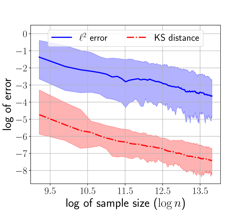
(a) Simulation: sample size

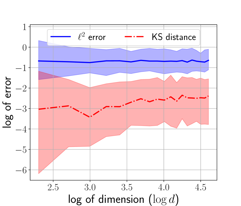
(b) Simulation: dimension

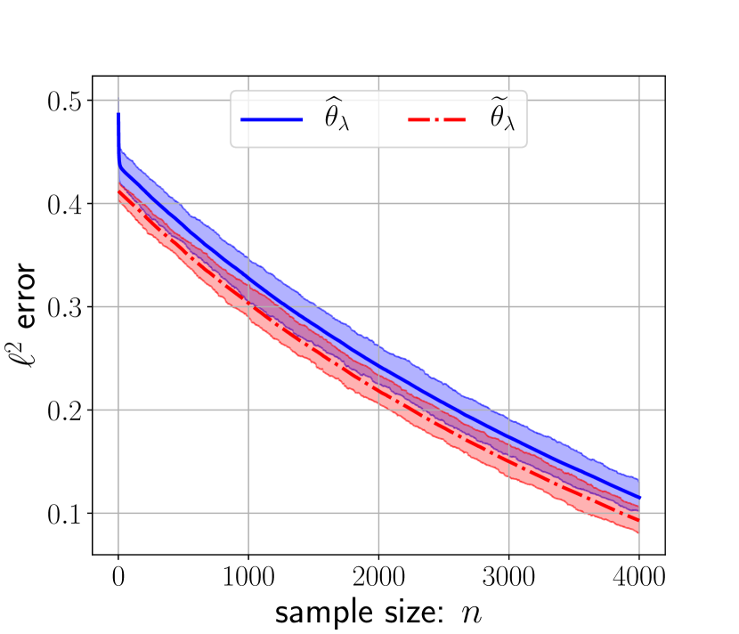
(c) Real data experiment

Figure 2: Means and confidence intervals of estimation errors in simulation and real data experiments. These plots demonstrate that the estimation error of our proposed estimator scales desirably with the sample size and dimension.

10.2 Real data experiments

We also evaluate the performance of our estimator (2) on a dataset on financial wealth and 401(k) plan participation of size $9,915$ from the R package ‘hdm’ (Chernozhukov et al., 2016) collected during wave 4 of the 1990 Survey of Income and Program Participation (SIPP). Similar to Chernozhukov and Hansen (2004); Kallus et al. (2019), we use participation in 401(k), age, income, family size, education, marital status, two-earner status, defined benefit (DB) pension status, IRA participation status, and homeownership status as contexts $x$ ($d=10$), and net financial assets as samples $y$ from the target CDF function. We split the whole dataset into two parts. To construct the basis $\Phi$, we use $1/3$ of the dataset to fit a Gaussian linear model for each context $x_{i}$ individually, and obtain a coefficient $\beta_{i}^{(1)}$, intercept $\beta_{i}^{(0)}$, and variance of residuals $\sigma_{i}^{2}$ for $i\in[d]$. Then, we define $\phi_{i}(x,t)$ to be the CDF of the Gaussian distribution $N(\beta^{(1)}_{i}x_{i}+\beta^{(0)}_{0},\sigma_{i}^{2})$. To evaluate the performance, we calculate $\widehat{\theta}_{\lambda}$ using (3) with $\mathfrak{m}=\gamma_{0,100}$ and $\lambda=10$ on a subset of size $n$ of the remaining $6,610$ data points, and denote the estimated parameter by $\widehat{\theta}_{\lambda}^{(n)}$. We use $\widetilde{\theta}_{\lambda}^{(n)}$ to denote the $\ell^{2}$ projection of $\widehat{\theta}_{\lambda}^{(n)}$ onto the probability simplex. Then, we calculate the $\ell^{2}$ errors $\|\widehat{\theta}_{\lambda}^{(n)}-\widehat{\theta}_{\lambda}^{(N)}\|$ and $\|\widetilde{\theta}_{\lambda}^{(n)}-\widetilde{\theta}_{\lambda}^{(N)}\|$ fixing $N=6,610$. This time, to get stable results, we permute the dataset uniformly at random independently, and repeat the above procedure $100$ times to obtain the means and $90\%$ confidence intervals of the $\ell^{2}$ errors that are plotted in Figure 2(c) against sample size $n$ ranging from $1$ to $4,000$. As shown in Figure 2(c), our estimator (2) generalizes quite well on real data, and the projected estimator $\widetilde{\theta}_{\lambda}$ has smaller error than (2) (as expected).

11 Conclusion

In this paper, we propose a linear model for contextual CDFs and an estimator for the coefficient parameter in this model. We prove $\widetilde{O}(\sqrt{d/n})$ upper bounds on the estimation error of our estimator under the adversarial and random settings, and show that the upper bounds are tight up to logarithmic factors by proving $\Omega(\sqrt{d/n})$ information theoretic lower bounds. Furthermore, when a mismatch exists in the linear model, we prove that the estimation error of our estimator only increases by an amount commensurate with the mismatch error. Our current work has the limitation that the bases are completely known. So, a fruitful future research direction would be to focus on the basis selection problem for CDF regression with possibly infinitely many base functions.

Appendix A Discussion on the minimax lower bound for the estimation of CDFs

First, for any contextual CDFs $F_{1}$ and $F_{2}$, define the uniform KS distance by

$$\textup{KS}(F_{1},F_{2}):=\sup_{x\in\mathcal{X}}\textup{KS}(F_{1}(x,\cdot),F_{2}(x,\cdot)).$$

Similar to the minimax $\ell^{2}$-risk defined in (12), we can define the minimax risk in terms of the uniform KS distance for the estimation of the contextual CDF $F$. For any distribution family $\mathcal{Q}$ and the contextual CDF function $\Xi:\mathcal{Q}\rightarrow[0,1]^{\mathcal{X}\times\mathbb{R}}$, the minimax risk in terms of the uniform KS distance is defined as

$$\mathfrak{R}(\Xi(\mathcal{Q});\textup{KS}):=\inf_{\hat{\Xi}}\sup_{Q\in\mathcal{Q}}\mathbb{E}_{z\sim Q}[\textup{KS}(\hat{\Xi}(z),\Xi(Q))].$$

We follow the notation in Section 4. With a slight abuse of notation, let $F(P)=\theta(P)^{\top}\Phi$. For the random setting, define the distribution family $\mathcal{P}_{0}:=\big{\{}\otimes_{j=1}^{n}P_{X}^{(j)}P_{Y|X;\theta}:\theta\in\mathbb{R}^{d},\ P_{X}^{(j)}\in\mathcal{D}_{\mathcal{X}}\textup{ such that }\mu_{\min}(\Sigma_{n})=0\big{\}}$. Then, we have the following results.

Proposition 24.

For any sequence $x^{1:n}\allowbreak=(x^{(1)},\dots,x^{(n)})\in\mathcal{X}^{n}$ such that $\mu_{\min}(U_{n})=0$, we have

$$\mathfrak{R}(F(\mathcal{P}_{x^{1:n}});\textup{KS})=\Omega\left(1\right).$$ (80)

For the random setting (Scheme II), we have

$$\mathfrak{R}(F(\mathcal{P}_{0});\textup{KS})=\Omega\left(1\right).$$ (81)

Proof of Proposition 24.

According to the discussion below Theorem 8, the discussion above Corollary 9, and Appendix 8.2, it suffices to show (80) under the fixed design setting.

Let us consider the fixed design setting where $\phi_{i}(x,\cdot)$ are the CDFs of Bernoulli distributions for $i\in[d]$, $d\geq 2$. Let $q_{ji}$ denote the zero probability of the Bernoulli distribution with CDF $\phi_{i}(x^{(j)},\cdot)=\Phi_{ji}(\cdot)$. We set $S=[0,1]$ and $\mathfrak{m}=\mathsf{Leb}$. Then, we have $U_{n}=\sum_{j=1}^{n}q_{j}q_{j}^{\top}$ where $q_{j}=[q_{j1},\dots,q_{jd}]^{\top}$.

For any $\theta_{*}\in\Delta^{d-1}$, we have $F(x^{(j)},t)=\theta_{*}^{\top}q_{j}$ under model (1) for any $t\in[0,1)$. Suppose that $q_{ji}=q_{11}\in[0,1]$ for any $i\in[d]$ and $j\in[n]$. Then for any $\theta_{*}\in[0,1]$, the samples $y^{(j)}$’s for $j\in[n]$ are generated from the same distribution which is the Bernoulli distribution with success probability $1-q_{11}$. We have $\mu_{\min}(U_{n})=0$. Thus, the condition of the proposition is satisfied.

For $n+1$, suppose that $q_{n+1,1}=1$ and $q_{n+1,2}=0$. Then, for any estimate $\check{F}_{n}$ of $F$, we have $\check{F}_{n}(x^{(n+1)},1/2)\in[0,1]$. If $\check{F}_{n}(x^{(n+1)},1/2)\in[0,1/2]$, consider the case where $\theta_{*}=\theta^{(1)}=[1,0,\dots,0]^{\top}$. Then, we have $|\check{F}_{n}(x^{(n+1)},1/2)-F(x^{(n+1)},1/2)|\geq 1/2$. If $\check{F}_{n}(x^{(n+1)},1/2)\in(1/2,1]$, consider the case where $\theta_{*}=\theta^{(2)}=[0,1,\dots,0]^{\top}$. Then, we also have $|\check{F}_{n}(x^{(n+1)},1/2)-F(x^{(n+1)},1/2)|\geq 1/2$. Thus, we have

$$\mathfrak{R}(F(\mathcal{P}_{x^{1:n}});\textup{KS})=\inf_{\check{F}_{n}}\sup_{P\in\mathcal{P}_{x^{1:(n)}}}\textup{KS}(\check{F}_{n},F)=\Omega(1).$$

Thus, the minimax risk in terms of the uniform KS distance of any estimate of $F$ is $\Omega(1)$. ∎

Recall that according to the discussion at the end of Section 3.2, for the plug-in estimate $\widehat{F}_{\lambda}$ of $F$ using our projected estimator $\widetilde{\theta}_{\lambda}$, we have the $\widetilde{O}(\min\{1,d/\sqrt{1+\mu_{\min}(U_{n})}\})$ upper bound in terms of the uniform KS distance. Proposition 24 implies that this plug-in estimate $\widehat{F}_{\lambda}$ is minimax optimal when $\mu_{\min}(U_{n})=0$.

It is worth noting that with the assumption that $\mu_{\min}(U_{n})=\Theta(n)$, the

$$\widetilde{O}(\min\{1,d/\sqrt{1+\mu_{\min}(U_{n})}\})=\widetilde{O}(d/\sqrt{n})$$

upper bound of $\widehat{F}_{\lambda}$ implies that the minimax lower bound in estimating $F$ is improved. Thus, we can see that $\mu_{\min}(U_{n})$ or $\mu_{\min}(\Sigma_{n})$ plays an important role in the estimation of $F$.

Appendix B Proof of Lemma 6

Proof.

For any $n\in\mathbb{N}$, define $\Delta^{U}_{n}:=\|U_{n}-\Sigma_{n}\|$ and $Z_{j}:=\int_{S}\Phi_{j}\Phi_{j}^{\top}-\Sigma_{n}$ for $j\in[n]$. We have $\mathbb{E}[Z_{j}]=0$ and

$$\left\|\int_{S}\Phi_{j}\Phi_{j}^{\top}\right\|_{2}=\mu_{\max}\left(\int_{S}\Phi_{j}\Phi_{j}^{\top}\right)\leq\int_{S}\|\Phi_{j}\|_{2}^{2}\leq d,$$

$$\|\Sigma^{(j)}\|_{2}=\mu_{\max}\left(\Sigma^{(j)}\right)=\mu_{\max}\left(\mathbb{E}\left[\int_{S}\Phi_{j}\Phi_{j}^{\top}\right]\right)\leq\mathbb{E}\left[\int_{S}\|\Phi_{j}\|_{2}^{2}\right]\leq d.$$

Thus, for each $j\in[n]$, we have

$$\|Z_{j}\|\leq\max\left\{\left\|\int_{S}\Phi_{j}\Phi_{j}^{\top}\right\|_{2},\ \|\Sigma^{(j)}\|_{2}\right\}\leq d.$$

By (Tropp, 2012, Theorem 1.3), for any $a\geq 0$, we have

$$\mathbb{P}[\Delta_{n}^{U}\geq a]\leq d\exp\left(-\frac{a^{2}}{8nd^{2}}\right).$$

In other words, for any $\delta\in(0,1)$, with probability at least $1-\delta$, we have

$$\Delta_{n}^{U}\leq d\sqrt{8n\log(d/\delta)}.$$

Thus, we can set $\Delta_{n}^{U}(\delta)\geq d\sqrt{8n\log(d/\delta)}$. ∎

Appendix C Proofs of theoretical results in Section 6.2

In this section, we provide the proofs of the stated theoretical results in Section 6.2.

Proof of Lemma 12.

By Fubini’s theorem, for any $\theta\in\mathcal{L}^{2}(\Omega,\mathfrak{n})$, we have

$$(U_{n}\theta)(\omega)=\int_{\Omega}\theta(\omega^{\prime})\sum_{j=1}^{n}\int_{S}\Phi_{j}(\omega,t)\Phi_{j}(\omega^{\prime},t)\mathfrak{m}(dt)\mathfrak{n}(d\omega^{\prime}).$$

Define the function

$$u_{n}:\Omega^{2}\rightarrow\mathbb{R},\ (\omega,\omega^{\prime})\mapsto\sum_{j=1}^{n}\int_{S}\Phi_{j}(\omega,t)\Phi_{j}(\omega^{\prime},t)\mathfrak{m}(dt).$$

Then, we have $(U_{n}\theta)(\omega)=\int_{\Omega}u_{n}(\omega,\omega^{\prime})\theta(\omega^{\prime})\mathfrak{n}(d\omega^{\prime})$. Since $\Phi_{j}(\omega,t)\in[0,1]$ for any $\omega\in\Omega$, $t\in S$ and $\mathfrak{m}$ is a probability measure on $S$, we have $u_{n}(\omega,\omega^{\prime})\in[0,n]$ for any $\omega,\omega^{\prime}\in\Omega$ and

$$\int_{\Omega}\int_{\Omega}|u_{n}(\omega,\omega^{\prime})|^{2}\mathfrak{n}(d\omega)\mathfrak{n}(d\omega^{\prime})\leq n^{2}\mathfrak{n}(\Omega)^{2}.$$

Thus, $u_{n}\in\mathcal{L}^{2}(\Omega^{2},\mathfrak{n}^{2})$ and $U_{n}$ is Hilbert-Schmidt integral operator for any $n\in\mathbb{N}$. Thus, it is also a compact operator.

Because $u_{n}(\omega,\omega^{\prime})=\sum_{j=1}^{n}\int_{S}\Phi_{j}(\omega,t)\Phi_{j}(\omega^{\prime},t)\mathfrak{m}(dt)=u_{n}(\omega^{\prime},\omega)\in\mathbb{R}$, $U_{n}$ is self-adjoint. For any $\theta\in\mathcal{L}^{2}(\Omega,\mathfrak{n})$, we have

$$\|U_{n}\theta\|^{2}= \int_{\Omega}\left|\int_{\Omega}\theta(\omega^{\prime})u_{n}(\omega,\omega^{\prime})\mathfrak{n}(d\omega^{\prime})\right|^{2}\mathfrak{n}(d\omega)$$

$$\leq \int_{\Omega}\int_{\Omega}|\theta(\omega^{\prime})|^{2}\mathfrak{n}(d\omega^{\prime})\int_{\Omega}|u_{n}(\omega,\omega^{\prime})|^{2}\mathfrak{n}(d\omega^{\prime})\mathfrak{n}(d\omega)$$

$$\leq n^{2}\mathfrak{n}(\Omega)^{2}\|\theta\|^{2}$$

and

$$\langle U_{n}\theta,\theta\rangle= \int_{\Omega}\int_{\Omega}u_{n}(\omega,\omega^{\prime})\theta(\omega^{\prime})\theta(\omega)\mathfrak{n}(\omega^{\prime})\mathfrak{n}(\omega)$$

$$= \sum_{j=1}^{n}\int_{S}\langle\theta(\cdot),\Phi_{j}(\cdot,t)\rangle^{2}\mathfrak{m}(dt)$$

$$\geq 0.$$

Thus, $U_{n}$ is a positive operator with $\|U_{n}\|\leq n\mathfrak{n}(\Omega)$. Note that $\langle U_{n}\theta,\theta\rangle=0$ iff $\langle\theta(\cdot),\Phi_{j}(\cdot,t)\rangle=0$ for $\mathfrak{m}$-a.e. $t\in S$ for all $j\in[n]$. Since $U_{n}$ is compact, if $\dim(\mathcal{L}^{2}(\Omega,\mathfrak{n}))=\infty$, $U_{n}$ is not invertible. ∎

Proof of Corollary 14.

By Lemma 12, since $\|U_{n}\|\leq n\mathfrak{n}(\Omega)$ and $U_{n}$ is positive, we have $0\leq\lambda_{i}=\langle e_{i},U_{n}e_{i}\rangle\leq n\mathfrak{n}(\Omega)$ for any $i\in\mathbb{N}$. Since $U_{n}$ is a compact operator and $\{e_{i}\}_{i\in\mathbb{N}}$ is an orthonormal basis consisting of eigenfunctions of $U_{n}$, by the Riesz-Schauder theorem (see e.g., Reed and Simon, 1972), we have that $\lambda_{i}\rightarrow 0$. ∎

Proof of Lemma 15.

For any $f,g\in\mathcal{L}^{2}_{\boldsymbol{\sigma}}(\Omega,\mathfrak{n})$ and $\alpha\in\mathbb{R}$, we have

$$\sum_{i=1}^{\infty}\frac{|\alpha\langle e_{i},f\rangle+\langle e_{i},g\rangle|^{2}}{\sigma_{i}^{4}}\leq \sum_{i=1}^{\infty}\frac{|\alpha|^{2}|\langle e_{i},f\rangle|^{2}+|\langle e_{i},g\rangle|^{2}+2|\alpha||\langle e_{i},f\rangle||\langle e_{i},g\rangle|}{\sigma_{i}^{4}}$$

$$\leq |\alpha|^{2}\sum_{i=1}^{\infty}\frac{|\langle e_{i},f\rangle|^{2}}{\sigma_{i}^{4}}+\sum_{i=1}^{\infty}\frac{|\langle e_{i},g\rangle|^{2}}{\sigma_{i}^{4}}+2|\alpha|\sqrt{\sum_{i=1}^{\infty}\frac{|\langle e_{i},f\rangle|^{2}}{\sigma_{i}^{4}}\sum_{i=1}^{\infty}\frac{|\langle e_{i},g\rangle|^{2}}{\sigma_{i}^{4}}}$$

$$< \infty$$

Then, we have $\alpha f+g\in\mathcal{L}^{2}_{\boldsymbol{\sigma}}(\Omega,\mathfrak{n})$ and $\mathcal{L}^{2}_{\boldsymbol{\sigma}}(\Omega,\mathfrak{n})$ is a linear subspace of $\mathcal{L}^{2}(\Omega,\mathfrak{n})$. ∎

Proof of Lemma 16.

For any $\alpha\in\mathbb{R}$ and $f,g\in\mathcal{L}_{\boldsymbol{\sigma}}^{2}(\Omega,\mathfrak{n})$, we have $\alpha f+g\in\mathcal{L}_{\boldsymbol{\sigma}}^{2}(\Omega,\mathfrak{n})$,

$$U_{n,\boldsymbol{\sigma}}(\alpha f+g)= \lim_{m\rightarrow\infty}\sum_{i=1}^{m}\left(\lambda_{i}+\frac{1}{\sigma_{i}^{2}}\right)\langle e_{i},\alpha f+g\rangle e_{i}$$

$$= \lim_{m\rightarrow\infty}\left[\alpha\sum_{i=1}^{m}\left(\lambda_{i}+\frac{1}{\sigma_{i}^{2}}\right)\langle e_{i},f\rangle e_{i}+\sum_{i=1}^{m}\left(\lambda_{i}+\frac{1}{\sigma_{i}^{2}}\right)\langle e_{i},g\rangle e_{i}\right]$$

$$= \alpha U_{n,\boldsymbol{\sigma}}f+U_{n,\boldsymbol{\sigma}}g,$$

and

$$\|U_{n,\boldsymbol{\sigma}}f\|^{2}= \sum_{i=1}^{\infty}\left(\lambda_{i}+\frac{1}{\sigma_{i}^{2}}\right)^{2}|\langle e_{i},f\rangle|^{2}$$

$$\geq \inf_{k\in\mathbb{N}}\left(\lambda_{k}+\frac{1}{\sigma_{k}^{2}}\right)^{2}\sum_{i=1}^{\infty}|\langle e_{i},f\rangle|^{2}$$

$$\geq \frac{1}{\sup_{k\in\mathbb{N}}\sigma_{k}^{4}}\|f\|^{2}$$

Thus, $U_{n,\boldsymbol{\sigma}}$ is a linear operator. Since $0\leq\sup_{i\in\mathbb{N}}\sigma_{i}^{2}<\infty$, we can conclude that $\|U_{n,\boldsymbol{\sigma}}f\|=0$ iff $f=0$. Therefore, $U_{n,\boldsymbol{\sigma}}$ is injective.

For any $\theta=\sum_{i=1}^{\infty}\langle e_{i},\theta\rangle e_{i}\in\mathcal{L}^{2}(\Omega,\mathfrak{n})$, we have

$$\sum_{i=1}^{\infty}\frac{\sigma_{i}^{4}|\langle e_{i},\theta\rangle|^{2}}{(1+\lambda_{i}\sigma_{i}^{2})^{2}}\leq\sup_{k\in\mathbb{N}}\sigma_{k}^{4}\sum_{i=1}^{\infty}|\langle e_{i},\theta\rangle|^{2}<\infty.$$

and

$$\sum_{i=1}^{\infty}\frac{|\langle e_{i},\theta\rangle|^{2}}{(1+\lambda_{i}\sigma_{i}^{2})^{2}}\leq\sum_{i=1}^{\infty}|\langle e_{i},\theta\rangle|^{2}<\infty.$$

Thus, we know that $\check{\theta}:=\sum_{i=1}^{\infty}\frac{\sigma_{i}^{2}\langle e_{i},\theta\rangle}{1+\lambda_{i}\sigma_{i}^{2}}e_{i}\in\mathcal{L}_{\boldsymbol{\sigma}}^{2}(\Omega,\mathfrak{n})$. Since

$$U_{n,\boldsymbol{\sigma}}\check{\theta}=\sum_{i=1}^{\infty}\left(\lambda_{i}+\frac{1}{\sigma_{i}^{2}}\right)\frac{\sigma_{i}^{2}\langle e_{i},\theta\rangle}{1+\lambda_{i}\sigma_{i}^{2}}e_{i}=\sum_{i=1}^{\infty}\langle e_{i},\theta\rangle e_{i}=\theta,$$

we can conclude that

$$U_{n,\boldsymbol{\sigma}}^{-1}\theta=\check{\theta}=\sum_{i=1}^{\infty}\frac{\sigma_{i}^{2}\langle e_{i},\theta\rangle}{1+\lambda_{i}\sigma_{i}^{2}}e_{i}$$

and $U_{n,\boldsymbol{\sigma}}$ is a bijective linear operator from $\mathcal{L}_{\boldsymbol{\sigma}}^{2}(\Omega,\mathfrak{n})$ onto $\mathcal{L}^{2}(\Omega,\mathfrak{n})$. Then, $U_{n,\boldsymbol{\sigma}}^{-1}$ exists as a bijective linear operator from $\mathcal{L}^{2}(\Omega,\mathfrak{n})$ onto $\mathcal{L}_{\boldsymbol{\sigma}}^{2}(\Omega,\mathfrak{n})$. Since for any $f\in\mathcal{L}_{\boldsymbol{\sigma}}^{2}(\Omega,\mathfrak{n})$, we have proved that $\|f\|\leq\sup_{k\in\mathbb{N}}\sigma_{k}^{2}\|U_{n,\boldsymbol{\sigma}}f\|$, we have $\|U_{n,\boldsymbol{\sigma}}^{-1}\|\leq\sup_{i\in\mathbb{N}}\sigma_{i}^{2}$ and $U_{n,\boldsymbol{\sigma}}^{-1}$ is a bounded linear operator on $\mathcal{L}^{2}(\Omega,\mathfrak{n})$. ∎

Proof of Lemma 17.

Since $\lim_{i\rightarrow\infty}\sigma_{i}=0$, there exists some $N\in\mathbb{N}$ such that $\sigma_{i}\leq 1$ for any $i\geq N$. Then, for any $\theta\in\mathcal{H}_{\boldsymbol{\sigma},\boldsymbol{e}}$, we have

$$\sum_{i=1}^{\infty}\frac{|\langle e_{i},\theta\rangle|^{2}}{\sigma_{i}^{4}}\leq \sum_{i=1}^{N}\frac{|\langle e_{i},\theta\rangle|^{2}}{\sigma_{i}^{4}}+\sum_{i=N+1}^{\infty}\frac{|\langle e_{i},\theta\rangle|^{2}}{\sigma_{i}^{2}}\leq\sum_{i=1}^{N}\frac{|\langle e_{i},\theta\rangle|^{2}}{\sigma_{i}^{4}}+\sum_{i=1}^{\infty}\frac{|\langle e_{i},\theta\rangle|^{2}}{\sigma_{i}^{2}}<\infty.$$

Thus, we have $\theta\in\mathcal{L}^{2}_{\boldsymbol{\sigma}}(\Omega,\mathfrak{n})$. ∎

Appendix D Proof of Proposition 18

Proof.

First, we show that $\sum_{j=1}^{n}\int_{S}\textup{I}_{y^{(j)}}(t)\Phi_{j}(\cdot,t)\mathfrak{m}(dt)\in\mathcal{L}^{2}(\Omega,\mathfrak{n})$. Indeed, we have

$$\|\sum_{j=1}^{n}\int_{S}\textup{I}_{y^{(j)}}(t)\Phi_{j}(\cdot,t)\mathfrak{m}(dt)\|^{2}\leq \sum_{j=1}^{n}\|\int_{S}\textup{I}_{y^{(j)}}(t)\Phi_{j}(\cdot,t)\mathfrak{m}(dt)\|^{2}$$

$$\leq \sum_{j=1}^{n}\|\int_{S}|\textup{I}_{y^{(j)}}(t)\Phi_{j}(\cdot,t)|\mathfrak{m}(dt)\|^{2}$$

$$\leq n\mathfrak{n}(\Omega)$$

$$\leq \infty.$$

Define $\theta_{0}:=U_{n,\boldsymbol{\sigma}}^{-1}\left(\sum_{j=1}^{n}\int_{S}\textup{I}_{y^{(j)}}(t)\Phi_{j}(\cdot,t)\mathfrak{m}(dt)\right)$. We show that $\theta_{0}\in\mathcal{L}^{2}_{\boldsymbol{\sigma}}(\Omega,\mathfrak{n})$. Then, by Lemma 17, we have $\theta_{0}\in\mathcal{H}_{\boldsymbol{\sigma},\boldsymbol{e}}$. Since $\lambda_{i}\geq 0$ for any $i\in\mathbb{N}$, we have

$$\sum_{i=1}^{\infty}\frac{1}{\sigma_{i}^{4}}|\langle e_{i},\theta\rangle|^{2} \leq\sum_{i=1}^{\infty}\left(\lambda_{i}+\frac{1}{\sigma_{i}^{2}}\right)^{2}|\langle e_{i},\theta_{0}\rangle|^{2}$$

$$\leq\|U_{n,\boldsymbol{\sigma}}\theta_{0}\|^{2}$$

$$=\|\sum_{j=1}^{n}\int_{S}\textup{I}_{y^{(j)}}(t)\Phi_{j}(\cdot,t)\mathfrak{m}(dt)\|^{2}<\infty.$$

Thus, $\theta_{0}\in\mathcal{L}^{2}_{\boldsymbol{\sigma}}(\Omega,\mathfrak{n})$. Then, for any $j\in[n]$, we have

$$|\Psi_{j}(\theta_{0},t)|= |\langle\theta_{0}(\cdot),\Phi_{j}(\cdot,t)\rangle|$$

$$\leq \int_{\Omega}|\theta_{0}(\omega)\Phi_{j}(\omega,t)|\mathfrak{n}(d\omega)$$

$$\leq \|\theta_{0}\|\|\Phi_{j}(\cdot,t)\|$$

$$\leq \sqrt{\mathfrak{n}(\Omega)}\|\theta_{0}\|$$

$$< \infty,$$

which implies that

$$L(\theta_{0};\boldsymbol{\sigma})=\sum_{j=1}^{n}\|\textup{I}_{y^{(j)}}(\cdot)-\Psi_{j}(\theta_{0},t)\|_{\mathcal{L}^{2}(S,\mathfrak{m})}+\|\theta_{0}\|_{\boldsymbol{\sigma},\boldsymbol{e}}<\infty$$

since $\mathfrak{m}(S)=1$ and $|\textup{I}_{y^{(j)}}(t)|\leq 1$ for any $j\in[n]$ and $t\in S$.

For any $\theta\in\mathcal{H}_{\boldsymbol{\sigma},\boldsymbol{e}}$, we have

$$L(\theta_{0}+\theta;\boldsymbol{\sigma})= L(\theta_{0})+\sum_{j=1}^{n}\int_{S}|\Psi_{j}(\theta,t)|^{2}\mathfrak{m}(dt)+\sum_{i=1}^{\infty}\frac{|\langle e_{i},\theta\rangle|^{2}}{\sigma_{i}^{2}}$$

$$+\sum_{j=1}^{n}\int_{S}\Psi_{j}(\theta,t)(\Psi_{j}(\theta_{0},t)-\textup{I}_{y^{(j)}}(t))\mathfrak{m}(dt)+\sum_{i=1}^{\infty}\frac{\langle e_{i},\theta\rangle\langle e_{i},\theta_{0}\rangle}{\sigma_{i}^{2}}.$$

Notice that by Fubini’s theorem, we have

$$\sum_{j=1}^{n}\int_{S}\Psi_{j}(\theta,t)\Psi_{j}(\theta_{0},t)\mathfrak{m}(dt)= \sum_{j=1}^{n}\int_{S}\int_{\Omega}\int_{\Omega}\theta(\omega)\Phi_{j}(\omega,t)\theta_{0}(\omega^{\prime})\Phi_{j}(\omega^{\prime},t)\mathfrak{n}(d\omega^{\prime})\mathfrak{n}(d\omega)\mathfrak{m}(dt)$$

$$= \int_{\Omega}\theta(\omega)\int_{\Omega}\theta_{0}(\omega^{\prime})\left(\sum_{j=1}^{n}\int_{S}\Phi_{j}(\omega,t)\Phi_{j}(\omega^{\prime},t)\mathfrak{m}(dt)\right)\mathfrak{n}(d\omega^{\prime})\mathfrak{n}(d\omega)$$

$$= \int_{\Omega}\theta(\omega)\int_{\Omega}\theta_{0}(\omega^{\prime})u_{n}(\omega,\omega^{\prime})\mathfrak{n}(d\omega^{\prime})\mathfrak{n}(d\omega)$$

$$= \langle\theta,U_{n}\theta_{0}\rangle,$$

$$\sum_{j=1}^{n}\int_{S}\Psi_{j}(\theta,t)\textup{I}_{y^{(j)}}(t)\mathfrak{m}(dt)= \sum_{j=1}^{n}\int_{S}\int_{\Omega}\theta(\omega)\Phi_{j}(\omega,t)\textup{I}_{y^{(j)}}(t)\mathfrak{n}(d\omega)\mathfrak{m}(dt)$$

$$= \int_{\Omega}\theta(\omega)\left(\sum_{j=1}^{n}\int_{S}\textup{I}_{y^{(j)}}(t)\Phi_{j}(\omega,t)\mathfrak{m}(dt)\right)\mathfrak{n}(d\omega)$$

$$= \langle\theta(\cdot),\sum_{j=1}^{n}\int_{S}\textup{I}_{y^{(j)}}(t)\Phi_{j}(\cdot,t)\mathfrak{m}(dt)\rangle,$$

and

$$\sum_{i=1}^{\infty}\frac{\langle e_{i},\theta\rangle\langle e_{i},\theta_{0}\rangle}{\sigma_{i}^{2}}= \sum_{i=1}^{\infty}\langle\theta,\frac{\langle e_{i},\theta_{0}\rangle}{\sigma_{i}^{2}}e_{i}\rangle$$

Since we have proved that

$$\sum_{i=1}^{\infty}\frac{|\langle e_{i},\theta_{0}\rangle|^{2}}{\sigma_{i}^{4}}<\infty,$$

we can conclude that $\sum_{i=1}^{\infty}\langle\theta,\frac{\langle e_{i},\theta_{0}\rangle}{\sigma_{i}^{2}}e_{i}\rangle=\langle\theta,\sum_{i=1}^{\infty}\frac{\langle e_{i},\theta_{0}\rangle}{\sigma_{i}^{2}}e_{i}\rangle$. Thus,

$$\sum_{j=1}^{n}\int_{S}\Psi_{j}(\theta,t)(\Psi_{j}(\theta_{0},t)-\textup{I}_{y^{(j)}}(t))\mathfrak{m}(dt)+\sum_{i=1}^{\infty}\frac{\langle e_{i},\theta\rangle\langle e_{i},\theta_{0}\rangle}{\sigma_{i}^{2}}$$

$$= \langle\theta(\cdot),(U_{n}\theta_{0})(\cdot)+\sum_{i=1}^{\infty}\frac{\langle e_{i},\theta_{0}\rangle}{\sigma_{i}^{2}}e_{i}(\cdot)-\sum_{j=1}^{n}\int_{S}\textup{I}_{y^{(j)}}(t)\Phi_{j}(\cdot,t)\mathfrak{m}(dt)\rangle$$

$$= \langle\theta(\cdot),(U_{n,\boldsymbol{\sigma}}\theta_{0})(\cdot)-\sum_{j=1}^{n}\int_{S}\textup{I}_{y^{(j)}}(t)\Phi_{j}(\cdot,t)\mathfrak{m}(dt)\rangle$$

$$= \langle\theta(\cdot),\sum_{j=1}^{n}\int_{S}\textup{I}_{y^{(j)}}(t)\Phi_{j}(\cdot,t)\mathfrak{m}(dt)-\sum_{j=1}^{n}\int_{S}\textup{I}_{y^{(j)}}(t)\Phi_{j}(\cdot,t)\mathfrak{m}(dt)\rangle$$

$$= 0.$$

Then, we have

$$L(\theta_{0}+\theta;\boldsymbol{\sigma})= L(\theta_{0})+\sum_{j=1}^{n}\int_{S}|\Psi_{j}(\theta,t)|^{2}\mathfrak{m}(dt)+\sum_{i=1}^{\infty}\frac{|\langle e_{i},\theta\rangle|^{2}}{\sigma_{i}^{2}}\geq L(\theta_{0};\boldsymbol{\sigma}).$$

Since $\frac{1}{\sigma_{i}^{2}}>0$ for all $i\in\mathbb{N}$, we have that $\sum_{i=1}^{\infty}\frac{|\langle e_{i},\theta\rangle|^{2}}{\sigma_{i}^{2}}>0$ for any $\theta\in\mathcal{H}_{\boldsymbol{\sigma},\boldsymbol{e}}$ with $\theta\neq 0$. Since $L(\theta_{0};\boldsymbol{\sigma})<\infty$, we can conclude that $L(\theta;\boldsymbol{\sigma})>L(\theta_{0};\boldsymbol{\sigma})$ for any $\theta\in\mathcal{H}_{\boldsymbol{\sigma},\boldsymbol{e}}\backslash\{\theta_{0}\}$ and $\widehat{\theta}_{\boldsymbol{\sigma}}=\theta_{0}$. ∎

Appendix E Proof of Lemma 20

Proof.

By Vershynin (2018, Proposition 4.2.12), we have

$$P(\Delta^{d-1},d_{\ell^{2}},\delta)\geq\frac{\textup{Vol}(\Delta^{d-1})}{\textup{Vol}(B_{\delta}^{d-1}(0))}$$ (82)

where $B_{\delta}^{d-1}(0):=\{x\in\mathbb{R}^{d-1}:\|x\|_{2}\leq\delta\}$ and for any $E\subseteq\mathbb{R}^{d-1}$, $\textup{Vol}(E)$ is the volume of $E$ under the Lebesgue measure in $\mathbb{R}^{d-1}$. According to Stein (1966); DLMF , We have

$$\textup{Vol}(\Delta^{d-1})=\frac{\sqrt{d}}{(d-1)!},$$ (83)

$$\textup{Vol}(B_{\delta}^{d-1}(0))=\frac{(\sqrt{\pi}\delta)^{d-1}}{\Gamma(\frac{d+1}{2})}.$$ (84)

Thus,

$$P(\Delta^{d-1},d_{\ell^{2}},\delta) \geq\frac{\Gamma(\frac{d+1}{2})\sqrt{d}}{(d-1)!(\sqrt{\pi}\delta)^{d-1}}$$

$$=\frac{\Gamma(\frac{d+1}{2})\sqrt{d}}{\Gamma(d)(\sqrt{\pi}\delta)^{d-1}}.$$ (85)

When $d\geq 3$, we have $\frac{d+1}{2}\geq 2$ and $d\geq 2$. According to Batir (2008, Theorem 1.5), we have $2((x-1/2)/e)^{x-1/2}<\Gamma(x)<3((x-1/2)/e)^{x-1/2}$ for any $x\geq 2$. Thus, for $d\geq 3$, we have

$$\frac{\Gamma(\frac{d+1}{2})}{\Gamma(d)}>\frac{2}{3}\frac{\left(\frac{d}{2e}\right)^{d/2}}{\left(\frac{d-1/2}{e}\right)^{d-1/2}}.$$

We verify that the above inequality also holds when $d=2$. Therefore, for any $d\geq 2$, we have

$$\frac{\Gamma(\frac{d+1}{2})}{\Gamma(d)}>\frac{2}{3}\frac{\left(\frac{d}{2e}\right)^{d/2}}{\left(\frac{d-1/2}{e}\right)^{d-1/2}}$$

which implies that

$$P(\Delta^{d-1},d_{\ell^{2}},\delta) >\frac{2\sqrt{d}}{3(\sqrt{\pi}\delta)^{d-1}}\frac{\left(\frac{d}{2e}\right)^{d/2}}{\left(\frac{d-1/2}{e}\right)^{d-1/2}}$$

$$\geq\frac{2\sqrt{d}}{3(\sqrt{\pi}\delta)^{d-1}}\frac{\left(\frac{d}{2e}\right)^{d/2}}{\left(\frac{d}{e}\right)^{d-1/2}}$$

$$=\frac{2\sqrt{d}}{3(\sqrt{\pi}\delta)^{d-1}}\frac{1}{2^{d/2}}e^{\frac{d-1}{2}}d^{-\frac{d-1}{2}}.$$ (86)

Let $\delta=\delta_{0}=\frac{\sqrt{e}}{2\sqrt{\pi d}}\left(\frac{\sqrt{d}}{3}\right)^{\frac{1}{d-1}}\left(\frac{1}{\sqrt{2}}\right)^{\frac{d}{d-1}}$. Then, by (86), we have

$$P(\Delta^{d-1},d_{\ell^{2}},\delta_{0})>2^{d}$$

which is exactly (64). For $d\geq 2$, we have $\delta_{0}\geq\frac{\sqrt{e}}{4\sqrt{\pi d}}\left(\frac{\sqrt{d}}{3}\right)^{\frac{1}{d-1}}$. Consider the function $f(x)=\frac{1}{x-1}\log\left(\frac{\sqrt{x}}{3}\right)$ with $x\geq 2$. We have that

$$f^{\prime}(x)=\frac{1-\frac{1}{x}-\log x+2\log 3}{2(x-1)^{2}}.$$

Since the function $g:\ x\mapsto-\frac{1}{x}-\log x$ is a decreasing function when $x\geq 2$ and $f^{\prime}(2)>0$, $f^{\prime}(e^{5})<0$, we have that $f$ first increases and then decreases when $x$ increases from 2 to infinity. Since $\lim_{x\rightarrow\infty}f(x)=0$, $f(2)=\log(\sqrt{2}/3)$, we have that $f(x)\geq f(2)=\log(\sqrt{2}/3)$. Therefore, for any $d\geq 2$, we have $\left(\frac{\sqrt{d}}{3}\right)^{\frac{1}{d-1}}\geq\sqrt{2}/3$ and

$$\delta_{0}\geq\frac{\sqrt{2e}}{12\sqrt{\pi d}}$$

which gives (65). ∎

Appendix F Proofs of upper bounds for the mismatched model

In this Section, we prove Theorem 10 in Appendix F.1 and Corollary 11 in Appendix F.2.

F.1 Proof of Theorem 10

Proof.

In the setting of Theorem 10, the sample $\{(x^{(j)},y^{(j)})\}_{j\in\mathbb{N}}$ is generated according to Scheme I, and similar to setting of Section 7.1, we consider the underlying probability space for the sample to be $([0,1]^{\mathbb{N}},\mathcal{B}([0,1])^{\mathbb{N}},\mathbb{P})$ which is already defined at the beginning of Section 7.1. Define the random vector $\Xi$ to be the identity mapping from $[0,1]^{\mathbb{N}}$ onto itself as in Section 7.1. Then, $\Xi$ follows the uniform distribution on $[0,1]^{\mathbb{N}}$. Suppose $\{(x^{(j)},y^{(j)})\}_{j\in\mathbb{N}}$ is sampled according to Scheme I with $F$ defined in (15). Then, according to Bogachev (2007, Proposition 10.7.6), for each $j\in\mathbb{N}$, there exist some $(\mathcal{B}(\mathcal{X})\otimes\mathcal{B}(S))^{j-1}\otimes\mathcal{B}([0,1])/\mathcal{B}(\mathcal{X})$-measurable function $h_{X}^{(j)}:\ (\mathcal{X}\times S)^{j-1}\times[0,1]\rightarrow\mathcal{X}$ and $(\mathcal{B}(\mathcal{X})\otimes\mathcal{B}(S))^{j-1}\otimes\mathcal{B}(\mathcal{X})\otimes\mathcal{B}([0,1])/\mathcal{B}(S)$-measurable function $h_{Y}^{(j)}:\ (\mathcal{X}\times S)^{j-1}\times\mathcal{X}\times[0,1]\rightarrow S$ such that $x^{(j)}=h_{X}^{(j)}(x^{(1)},y^{(1)},\dots,x^{(j-1)},y^{(j-1)},\Xi^{(2j-1)})$, $y^{(j)}=h_{Y}^{(j)}(x^{(1)},y^{(1)},\dots,x^{(j-1)},y^{(j-1)},x^{(j)},\Xi^{(2j)})$, and

$$\mathbb{E}\left[\mathbbm{1}\left\{h_{Y}^{(j)}(x^{(1)},y^{(1)},\dots,x^{(j-1)},y^{(j-1)},x^{(j)},\Xi^{(2j)})\leq t\right\}\big{|}\mathcal{F}_{j-1}\right]=\theta_{*}^{\top}\Phi(x^{(j)},t)+e(x^{(j)},t)$$ (87)

for any $t\in S$ and $j\in\mathbb{N}$, where $\mathcal{F}_{j}:=\sigma\left(\big{\{}\Xi^{(k)}:k\in[2j+1]\big{\}}\right)$. With the same proof provided at the beginning of Section 7.1, $\left\{y^{(j)}\right\}_{j\in\mathbb{N}}$ is $\left\{\mathcal{F}_{j}\right\}_{j\in\mathbb{N}}$-adapted, $x^{(j)}$ is $\mathcal{F}_{j-1}/\mathcal{B}(\mathcal{X})$-measurable, and $\Phi_{j}$ is $(\mathcal{F}_{j-1}\otimes\mathcal{B}(S))/\mathcal{B}([0,1]^{d})$-measurable for each $j\in\mathbb{N}$. Since $e:$ $\mathcal{X}\times S\rightarrow[-1,1]$, $(x,t)\mapsto e(x,t)$ is $\mathcal{B}(\mathcal{X})\otimes\mathcal{B}(S)$-measurable and $x^{(j)}$ is $\mathcal{F}_{j-1}/\mathcal{B}(\mathcal{X})$-measurable, we have that $e_{j}:$ $[0,1]^{\mathbb{N}}\times S\rightarrow[-1,1]$, $(\xi,t)\mapsto e(x^{(j)}(\xi),t)$ is $\mathcal{F}_{j-1}\otimes\mathcal{B}(S)$-measurable.

Define $V_{j}:=\int_{S}\textup{I}_{y^{(j)}}\Phi_{j}-\int_{S}(\theta_{*}^{\top}\Phi_{j}+e_{j})\Phi_{j}$. Since $\textup{I}_{y^{(j)}}$ is $\mathcal{F}_{j}\otimes\mathcal{B}(S)$-measurable and $e_{j}$ and $\Phi_{j}$ are $\mathcal{F}_{j-1}\otimes\mathcal{B}(S)$-measurable, by Fubini’s theorem and (87), We have

$$\mathbb{E}[V_{j}|\mathcal{F}_{j-1}]= \mathbb{E}\left[\int_{S}\textup{I}_{y^{(j)}}\Phi_{j}\Big{|}\mathcal{F}_{j-1}\right]-\int_{S}(\theta_{*}^{\top}\Phi_{j}+e_{j})\Phi_{j}$$

$$= \int_{S}\mathbb{E}\left[\textup{I}_{y^{(j)}}|\mathcal{F}_{j-1}\right]\Phi_{j}-\int_{S}(\theta_{*}^{\top}\Phi_{j}+e_{j})\Phi_{j}$$

$$= \int_{S}(\theta_{*}^{\top}\Phi_{j}+e_{j})\Phi_{j}-\int_{S}(\theta_{*}^{\top}\Phi_{j}+e_{j})\Phi_{j}$$

$$= 0.$$

For any $\alpha\in\mathbb{R}^{d}$, if $n=0$, define $M_{n}(\alpha)=1$. If $n\geq 1$, define $M_{n}(\alpha):=\exp\left\{\alpha^{\top}W_{n}-\frac{1}{2}\|\alpha\|^{2}_{U_{n}}\right\}$ for $W_{n}:=\sum_{j=1}^{n}V_{j}$ and $U_{n}=\sum_{j=1}^{n}\int_{S}\Phi_{j}\Phi_{j}^{\top}$. Then, with the similar proof as in Appendix 7.1.1, we can show that $W_{n}$ is $\mathcal{F}_{n}$-measurable, $U_{n}$ is $\mathcal{F}_{n-1}$-measurable, and $M_{n}$ is $\mathcal{F}_{n}\otimes\mathcal{B}(\mathbb{R}^{d})$-measurable for any $n\in\mathbb{N}$. Thus, for any $\alpha\in\mathbb{R}^{d}$, $\{M_{n}(\alpha)\}_{n\geq 0}$ is $\{\mathcal{F}_{n}\}_{n\geq 0}$-adapted. Moreover, for any $\alpha\in\mathbb{R}^{d}$ and $n\in\mathbb{N}$, we have

$$\mathbb{E}[M_{n}(\alpha)|\mathcal{F}_{n-1}]= M_{n-1}(\alpha)\mathbb{E}\left[\exp\left\{\alpha^{\top}V_{n}-\frac{1}{2}\alpha^{\top}\left(\int_{S}\Phi_{n}\Phi_{n}^{\top}\right)\alpha\right\}\Big{|}\mathcal{F}_{n-1}\right]$$

$$= M_{n-1}(\alpha)\frac{\mathbb{E}\left[\exp\left\{\alpha^{\top}V_{n}\right\}|\mathcal{F}_{n-1}\right]}{\exp\left\{\frac{1}{2}\int_{S}\left(\alpha^{\top}\Phi_{n}\right)^{2}\right\}}.$$ (88)

Since $-\int_{S}|\alpha^{\top}\Phi_{n}|\leq\alpha^{\top}V_{n}\leq\int_{S}|\alpha^{\top}\Phi_{n}|$ a.s., we have

$$\mathbb{E}\left[\exp\left\{\alpha^{\top}V_{n}\right\}|\mathcal{F}_{n-1}\right] \leq\exp\left\{\frac{4}{8}\left(\int_{S}|\alpha^{\top}\Phi_{n}|\right)^{2}\right\}$$

$$\leq\exp\left\{\frac{1}{2}\int_{S}\left(\alpha^{\top}\Phi_{n}\right)^{2}\right\}$$ (89)

$$\leq\exp\left\{\frac{1}{2}\int_{S}\left(\alpha^{\top}\Phi_{n}\right)^{2}\right\}$$ (90)

where (89) is by Cauchy-Schwarz inequality and $\int_{S}1=\mathfrak{m}(S)=1$. Then, by (88) and (90), we have

$$\mathbb{E}[M_{n}(\alpha)|\mathcal{F}_{n-1}]\leq M_{n-1}(\alpha)\frac{\exp\left\{\frac{1}{2}\int_{S}\left(\alpha^{\top}\Phi_{n}\right)^{2}\right\}}{\exp\left\{\frac{1}{2}\int_{S}\left(\alpha^{\top}\Phi_{n}\right)^{2}\right\}}=M_{n-1}(\alpha).$$

Thus, for any $\alpha\in\mathbb{R}^{d}$, $\{M_{n}(\alpha)\}_{n\geq 0}$ is a super-martingale.

Now define $\widebar{M}_{n}:=\int_{\mathbb{R}^{d}}M_{n}(\alpha)h(\alpha)d\alpha$ for

$$h(\alpha)=\left(\frac{\lambda}{2\pi}\right)^{\frac{d}{2}}\exp\left\{-\frac{\lambda}{2}\alpha^{\top}\alpha\right\}=\left(\frac{\lambda}{2\pi}\right)^{\frac{d}{2}}\exp\left\{-\frac{1}{2}\|\alpha\|^{2}_{\lambda I_{d}}\right\}.$$

Then, with the same calculation as (33) in Section 7.1.1, we have $\widebar{M}_{n}=\frac{\lambda^{d/2}}{\det(U_{n}(\lambda))^{1/2}}\allowbreak\exp\left(\frac{1}{2}\|W_{n}\|_{U_{n}(\lambda)^{-1}}^{2}\right)$. By Fubini’s theorem, $M_{n}$ is $\mathcal{F}_{n}\otimes\mathcal{B}(\mathbb{R}^{d})$-measurable implies that $\widebar{M}_{n}$ is $\mathcal{F}_{n}$-measurable for any $n\geq 0$. With the same analysis as (35), $\{\widebar{M}_{n}\}_{n\geq 0}$ is a super-martingale. By Doob’s maximal inequality for super-martingales, we have that

$$\mathbb{P}\left[\sup_{n\in\mathbb{N}}\widebar{M}_{n}\geq\delta\right]\leq\frac{\mathbb{E}[\widebar{M}_{0}]}{\delta}=\frac{1}{\delta}$$

which implies that for any $N\in\mathbb{N}$,

$$\mathbb{P}\left[\exists n\in[N]\text{ s.t. }\|W_{n}\|_{U_{n}(\lambda)^{-1}}\geq\sqrt{\log\frac{\det(U_{n}(\lambda))}{\lambda^{d}}+2\log\frac{1}{\delta}}\right]\leq\delta.$$

According to (40), we have

$$\|W_{n}\|_{U_{n}(\lambda)^{-1}}\leq\sqrt{d\log\left(1+\frac{n}{\lambda}\right)+2\log\frac{1}{\delta}}$$ (91)

for all $n\in\mathbb{N}$ with probability at least $1-\delta$.

By (3), (37), and the definition of $V_{j}$, we have

$$\widehat{\theta}_{\lambda}-\theta_{*}=U_{n}(\lambda)^{-1}\left(\sum_{j=1}^{n}V_{j}+E_{n}-\lambda\theta_{*}\right)=U_{n}(\lambda)^{-1}W_{n}+U_{n}(\lambda)^{-1}(E_{n}-\lambda\theta_{*}).$$ (92)

where $E_{n}=\sum_{j=1}^{n}\int_{S}e_{j}\Phi_{j}$ by definition. Thus,

$$\|\widehat{\theta}_{\lambda}-\theta_{*}\|_{U_{n}(\lambda)} \leq\|U_{n}(\lambda)^{-1}W_{n}\|_{U_{n}(\lambda)}+\|U_{n}(\lambda)^{-1}(E_{n}-\lambda\theta_{*})\|_{U_{n}(\lambda)}$$

$$\leq\|W_{n}\|_{U_{n}(\lambda)^{-1}}+\|\lambda\theta_{*}\|_{U_{n}(\lambda)^{-1}}+\|E_{n}\|_{U_{n}(\lambda)^{-1}}$$

$$\leq\|W_{n}\|_{U_{n}(\lambda)^{-1}}+\sqrt{\lambda}\|\theta_{*}\|+\|E_{n}\|_{U_{n}(\lambda)^{-1}}$$ (93)

where (93) is because of $U_{n}(\lambda)^{-1}=\frac{1}{\lambda}\left(I-U_{n}(\lambda)^{-1}U_{n}\right)$ and $\|I-U_{n}(\lambda)^{-1}U_{n}\|_{2}\leq 1$.

By (91) and (93), for any $\delta\in(0,1)$, with probability at least $1-\delta$, we have

$$\|\widehat{\theta}_{\lambda}-\theta_{*}\|_{U_{n}(\lambda)}\leq\sqrt{d\log\left(1+\frac{n}{\lambda}\right)+2\log\frac{1}{\delta}}+\sqrt{\lambda}\|\theta_{*}\|+\|E_{n}\|_{U_{n}(\lambda)^{-1}}.$$ (94)

for all $n\in\mathbb{N}$. Since $U_{n}(\lambda)-\lambda I_{d}$ is positive semi-definite, (94) immediately implies that

$$\|\widehat{\theta}_{\lambda}-\theta\|_{U_{n}(\lambda)}\leq\sqrt{d\log\left(1+\frac{n}{\lambda}\right)+2\log\frac{1}{\delta}}+\sqrt{\lambda}\|\theta_{*}\|+\frac{1}{\sqrt{\lambda}}\|E_{n}\|$$ (95)

which is exactly (16).

∎

F.2 Proof of Corollary 11

Proof.

In the setting of Corollary 11, the sample $\{(x^{(j)},y^{(j)})\}_{j\in\mathbb{N}}$ is generated according to Scheme II. In the following proof, we consider the underlying probability space for the sample $\{(x^{(j)},y^{(j)})\}_{j\in\mathbb{N}}$ to be $([0,1]^{\mathbb{N}},\mathcal{B}([0,1])^{\mathbb{N}},\mathbb{P})$ which has already been defined at the beginning of Section 7.1. Define the random vector $\Xi$ to be the identity mapping from $[0,1]^{\mathbb{N}}$ onto itself as in Section 7.1. Then, $\Xi$ follows the uniform distribution on $[0,1]^{\mathbb{N}}$. Suppose $\{(x^{(j)},y^{(j)})\}_{j\in\mathbb{N}}$ is sampled according to Scheme II with $F$ defined in (15). Then, according to Bogachev (2007, Proposition 10.7.6), for each $j\in\mathbb{N}$, there exist some $\mathcal{B}([0,1])/\mathcal{B}(\mathcal{X})$-measurable function $h_{X}^{(j)}:\ [0,1]\rightarrow\mathcal{X}$ and $\mathcal{B}(\mathcal{X})\otimes\mathcal{B}([0,1])/\mathcal{B}(S)$-measurable function $h_{Y}^{(j)}:\ \mathcal{X}\times[0,1]\rightarrow S$ such that $x^{(j)}=h_{X}^{(j)}(\Xi^{(2j-1)})$, $y^{(j)}=h_{Y}^{(j)}(x^{(j)},\Xi^{(2j)})$, and

$$\mathbb{E}\left[\mathbbm{1}\left\{h_{Y}^{(j)}(x^{(j)},\Xi^{(2j)})\leq t\right\}\big{|}\mathcal{F}_{j-1}\right]=\theta_{*}^{\top}\Phi(x^{(j)},t)+e(x^{(j)},t)$$ (96)

for any $t\in S$ and $j\in\mathbb{N}$, where $\mathcal{F}_{j}:=\sigma\left(\big{\{}\Xi^{(k)}:k\in[2j+1]\big{\}}\right)$. With the same proof provided at the beginning of Section 7.1, $\left\{y^{(j)}\right\}_{j\in\mathbb{N}}$ is $\left\{\mathcal{F}_{j}\right\}_{j\in\mathbb{N}}$-adapted and $\Phi_{j}$ is $(\mathcal{F}_{j-1}\otimes\mathcal{B}(S))/\mathcal{B}([0,1]^{d})$-measurable for each $j\in\mathbb{N}$. Moreover, $\{x^{(j)}\}_{j\in\mathbb{N}}$ is independent, which implies that $\{\Phi_{j}(t)\}_{j\in\mathbb{N}}$ is independent for any $t\in S$, $\{e_{j}(t)\}_{j\in\mathbb{N}}$ is independent for any $t\in S$, and $\{y^{(j)}\}_{j\in\mathbb{N}}$ is independent.

Let $b_{j}(t):=\mathbb{E}[e_{j}(t)\Phi_{j}(t)]$ for $t\in S$ and $j\in[n]$. Then, by Fubini’s theorem, $b_{j}$ is measurable with $b_{ji}(t)\in[-1,1]$ for $t\in S$, $j\in\mathbb{N}$ and $i\in[d]$. By definition and Fubini’s theorem, we have $B_{n}=\sum_{j=1}^{n}\int_{S}b_{j}$.

Define $V_{j}:=\int_{S}\textup{I}_{y^{(j)}}\Phi_{j}-\int_{S}\theta_{*}^{\top}\Phi_{j}\Phi_{j}-\int_{S}b_{j}$. By Fubini’s theorem and (96), we have

$$\mathbb{E}[V_{j}]= \mathbb{E}\left[\int_{S}(\textup{I}_{y^{(j)}}-\theta_{*}^{\top}\Phi_{j})\Phi_{j}\right]-\int_{S}b_{j}$$

$$= \int_{S}\mathbb{E}\left[(\textup{I}_{y^{(j)}}-\theta_{*}^{\top}\Phi_{j})\Phi_{j}\right]-\int_{S}b_{j}$$

$$= \int_{S}\mathbb{E}\left[\mathbb{E}[\textup{I}_{y^{(j)}}-\theta_{*}^{\top}\Phi_{j}|\mathcal{F}_{j-1}]\Phi_{j}\right]-\int_{S}b_{j}$$

$$= \int_{S}\mathbb{E}\left[e_{j}\Phi_{j}\right]-\int_{S}b_{j}$$

$$= \int_{S}b_{j}-\int_{S}b_{j}$$

$$= 0.$$

For any $\alpha\in\mathbb{R}^{d}$, if $n=0$, define $M_{n}(\alpha)=1$. If $n\geq 1$, define $M_{n}(\alpha):=\exp\left\{\alpha^{\top}W_{n}-\frac{1}{2}\|\alpha\|^{2}_{U_{n}}\right\}$ for $W_{n}:=\sum_{j=1}^{n}V_{j}$ and $U_{n}=\sum_{j=1}^{n}\int_{S}\Phi_{j}\Phi_{j}^{\top}$. Similar to Appendix F.1, we can show that $M_{n}$ is $\mathcal{F}_{n}\otimes\mathcal{B}(\mathbb{R}^{d})$-measurable for any $n\geq 0$. Moreover, for any $n\in\mathbb{N}$,

$$\mathbb{E}[M_{n}(\alpha)|\mathcal{F}_{n-1}]= M_{n-1}(\alpha)\mathbb{E}\left[\exp\left\{\alpha^{\top}V_{n}-\frac{1}{2}\alpha^{\top}\left(\int_{S}\Phi_{n}\Phi_{n}^{\top}\right)\alpha\right\}\Big{|}\mathcal{F}_{n-1}\right]$$

$$= M_{n-1}(\alpha)\frac{\mathbb{E}\left[\exp\left\{\alpha^{\top}V_{n}\right\}|\mathcal{F}_{n-1}\right]}{\exp\left\{\frac{1}{2}\int_{S}\left(\alpha^{\top}\Phi_{n}\right)^{2}\right\}}$$ (97)

with $-\int_{S}|\alpha^{\top}\Phi_{n}|-\int_{S}\alpha^{\top}b_{n}\leq\alpha^{\top}V_{n}\leq\int_{S}|\alpha^{\top}\Phi_{n}|-\int_{S}\alpha^{\top}b_{n}$ a.s.. Thus,

$$\mathbb{E}\left[\exp\left\{\alpha^{\top}V_{n}\right\}|\mathcal{F}_{n-1}\right] \leq\exp\left\{\frac{4}{8}\left(\int_{S}|\alpha^{\top}\Phi_{n}|\right)^{2}\right\}$$

$$\leq\exp\left\{\frac{1}{2}\int_{S}\left(\alpha^{\top}\Phi_{n}\right)^{2}\right\}$$

$$\leq\exp\left\{\frac{1}{2}\int_{S}\left(\alpha^{\top}\Phi_{n}\right)^{2}\right\}$$ (98)

Then, by (97) and (98), we have

$$\mathbb{E}[M_{n}(\alpha)|\mathcal{F}_{n-1}]\leq M_{n-1}(\alpha)\frac{\exp\left\{\frac{1}{2}\int_{S}\left(\alpha^{\top}\Phi_{n}\right)^{2}\right\}}{\exp\left\{\frac{1}{2}\int_{S}\left(\alpha^{\top}\Phi_{n}\right)^{2}\right\}}=M_{n-1}(\alpha).$$

Thus, for any $\alpha\in\mathbb{R}^{d}$, $\{M_{n}(\alpha)\}_{n\geq 0}$ is a super-martingale. With the same approach as in Appendix F.1, for any $\lambda\in(0,\infty)$, we can show that

$$\|\widehat{\theta}_{\lambda}-\theta_{*}\|_{U_{n}(\lambda)}\leq\sqrt{d\log\left(1+\frac{n}{\lambda}\right)+2\log\frac{1}{\delta}}+\sqrt{\lambda}\|\theta_{*}\|+\frac{1}{\sqrt{\lambda}}\|B_{n}\|$$ (99)

for all $n\in\mathbb{N}$ with probability at least $1-\delta$. Then, using the same analysis as in Appendix 7.2.2, we can show that for any $\delta_{1}\in(0,1)$, $\delta_{2}\in(0,1-\delta_{1})$, and $n\geq\frac{32d^{2}}{\sigma_{\min}^{2}}\log(d/\delta_{1})$, we have

$$\|\widehat{\theta}_{\lambda}-\theta_{*}\|_{\Sigma_{n}}\leq\sqrt{2\left(d\log\left(1+\frac{1}{\lambda}\right)+2\log\frac{1}{\delta_{2}}\right)}+\sqrt{2\lambda}\|\theta_{*}\|+\sqrt{\frac{2}{\lambda}}\|B_{n}\|$$

with probability at least $1-\delta_{1}-\delta_{2}$. Then, (17) is obtained by setting $\delta_{1}=\delta_{2}=\delta\in(0,1/2)$. ∎

Appendix G Proofs of the lemmas in Section 9

In this section, we provide the proofs of the technical lemmas in Section 9.

Proof of Lemma 22.

For any $n\in\mathbb{N}$, since $V_{j}$ is $\mathcal{F}_{\Omega}\otimes\mathcal{F}_{j}$-measurable for any $j\in[n]$ and $W_{n}=\sum_{j=1}^{n}V_{j}$, we have that $W_{n}$ is also $\mathcal{F}_{\Omega}\otimes\mathcal{F}_{j}$-measurable. According to the similar arguments as in Section 7.1.1, we know that $U_{n}$ is $\mathcal{F}_{\Omega}\otimes\mathcal{F}_{n-1}$-measurable. Thus, by Fubini’s theorem, for any $\alpha\in\mathcal{L}^{2}(\Omega,\mathfrak{n})$, $M_{n}(\alpha)=\exp\left\{\langle\alpha,W_{n}\rangle-\frac{1}{2}\|\alpha\|^{2}_{U_{n}}\right\}$ is $\mathcal{F}_{n}$-measurable, which implies that $\{M_{n}(\alpha)\}_{n\geq 0}$ is $\{\mathcal{F}_{n}\}_{n\geq 0}$-adapted. For any $n\in\mathbb{N}$, we have that

$$\mathbb{E}[M_{n}(\alpha)|\mathcal{F}_{n-1}]= M_{n-1}(\alpha)\mathbb{E}\left[\exp\left\{\langle\alpha,V_{n}\rangle-\frac{1}{2}\int_{S}\Psi_{n}(\alpha,t)^{2}\mathfrak{m}(dt)\right\}\Big{|}\mathcal{F}_{n-1}\right]$$

$$= M_{n-1}(\alpha)\frac{\mathbb{E}\left[\exp\left\{\langle\alpha,V_{n}\rangle\right\}|\mathcal{F}_{n-1}\right]}{\exp\left\{\frac{1}{2}\int_{S}\Psi_{n}(\alpha,t)^{2}\mathfrak{m}(dt)\right\}}.$$

Since $-\int_{S}|\Psi_{n}(\alpha,t)|\mathfrak{m}(dt)\leq\langle\alpha,V_{n}\rangle\leq\int_{S}|\Psi_{n}(\alpha,t)|\mathfrak{m}(dt)$, according to Hoeffding’s lemma (Hoeffding, 1963) and Cauchy-Schwarz inequality, we have

$$\mathbb{E}\left[\exp\left\{\langle\alpha,V_{n}\rangle\right\}|\mathcal{F}_{n-1}\right] \leq\exp\left\{\frac{4}{8}\left(\int_{S}|\Psi_{n}(\alpha,t)|\mathfrak{m}(dt)\right)^{2}\right\}$$

$$\leq\exp\left\{\frac{1}{2}\int_{S}\Psi_{n}(\alpha,t)^{2}\mathfrak{m}(dt)\right\}$$

$$\leq\exp\left\{\frac{1}{2}\int_{S}\Psi_{n}(\alpha,t)^{2}\mathfrak{m}(dt)\right\}.$$

Then, we have

$$\mathbb{E}[M_{n}(\alpha)|\mathcal{F}_{n-1}]\leq M_{n-1}(\alpha)\frac{\exp\left\{\frac{1}{2}\int_{S}\Psi_{n}(\alpha,t)^{2}\mathfrak{m}(dt)\right\}}{\exp\left\{\frac{1}{2}\int_{S}\Psi_{n}(\alpha,t)^{2}\mathfrak{m}(dt)\right\}}=M_{n-1}(\alpha).$$

Since $M_{0}(\alpha)=1$ and $M_{n}(\alpha)\geq 0$, for any $\alpha\in\mathcal{L}^{2}(\Omega,\mathfrak{n})$, $\{M_{n}(\alpha)\}_{n\geq 0}$ is a non-negative super-martingale. ∎

Proof of Lemma 23.

For any $m\in\mathbb{N}$, we have

$$|H_{\infty}-H_{m}|= \left|\sum_{i=m+1}^{\infty}(\beta_{i}w^{\prime}_{i}-\frac{1}{2}\lambda_{i}\beta_{i}^{2})\right|$$

$$\leq \sqrt{\sum_{i=m+1}^{\infty}\beta_{i}^{2}}\sqrt{\sum_{i=m+1}^{\infty}(w^{\prime}_{i})^{2}}+n\mathfrak{n}(\Omega)\sum_{i=m+1}^{\infty}\beta_{i}^{2}.$$

Since $\sum_{i=1}^{\infty}(w_{i}^{\prime})^{2}=\|W_{n}\|^{2}<\infty$ and $\sum_{i=1}^{\infty}\beta_{i}^{2}<\infty$ a.s., we have that $\lim_{m\rightarrow\infty}|H_{m}-H_{\infty}|=0$ a.s.. Thus,

$$\lim_{m\rightarrow\infty}\left|\exp(H_{m})-M_{n}(\beta)\right|=\lim_{m\rightarrow\infty}\left|\exp(H_{m})-\exp(H_{\infty})\right|=0.$$

Since $|W_{n}|\leq n$ a.s., we have

$$|\exp(H_{m})|\leq \exp\left(|\langle\beta,W_{n}\rangle|+\frac{1}{2}\|\beta\|_{U_{n}}^{2}\right)$$

$$\leq \exp\left(n\sum_{i=1}^{\infty}|\sigma_{i}\zeta_{i}|+\frac{1}{2}\sum_{i=1}^{\infty}\lambda_{i}\sigma_{i}^{2}\zeta_{i}^{2}\right)$$

for all $m\in\mathbb{N}$ a.s..

Moreover, for any $m\in\mathbb{N}$, by the independence of $\{\zeta_{i}\}_{i\in\mathbb{N}}$, if $|\sigma_{i}|<\frac{1}{\sqrt{\lambda_{i}}}$ for all $i\in\mathbb{N}$, then we have

$$\mathbb{E}\left[\exp\left(n\sum_{i=1}^{m}|\sigma_{i}\zeta_{i}|+\frac{1}{2}\sum_{i=1}^{m}\lambda_{i}\sigma_{i}^{2}\zeta_{i}^{2}\right)\right]$$

$$= \prod_{i=1}^{m}\mathbb{E}\left[\exp\left(|\sigma_{i}\zeta_{i}|+\frac{1}{2}\lambda_{i}\sigma_{i}^{2}\zeta_{i}^{2}\right)\right]$$

$$= \prod_{i=1}^{m}\exp\left(n|\sigma_{i}\zeta_{i}|+\frac{1}{2}(\lambda_{i}\sigma_{i}^{2}-1)\zeta_{i}^{2}\right)\frac{d\zeta_{i}}{\sqrt{2\pi}}$$

$$= \prod_{i=1}^{m}\frac{2}{\sqrt{1-\lambda_{i}\sigma_{i}^{2}}}\exp\left(\frac{n^{2}\sigma_{i}^{2}}{2(1-\lambda_{i}\sigma_{i}^{2})}\right)\Phi_{N(0,1)}\left(\frac{n|\sigma_{i}|}{\sqrt{1-\lambda_{i}\sigma_{i}^{2}}}\right)$$

where $\Phi_{N(0,1)}$ denotes the CDF of the $N(0,1)$ distribution. By the monotone convergence theorem, we have

$$\mathbb{E}\left[\exp\left(n\sum_{i=1}^{\infty}|\sigma_{i}\zeta_{i}|+\frac{1}{2}\sum_{i=1}^{\infty}\lambda_{i}\sigma_{i}^{2}\zeta_{i}^{2}\right)\right]$$

$$= \prod_{i=1}^{\infty}\frac{2}{\sqrt{1-\lambda_{i}\sigma_{i}^{2}}}\exp\left(\frac{n^{2}\sigma_{i}^{2}}{2(1-\lambda_{i}\sigma_{i}^{2})}\right)\Phi_{N(0,1)}\left(\frac{n|\sigma_{i}|}{\sqrt{1-\lambda_{i}\sigma_{i}^{2}}}\right)$$

$$\leq \frac{1}{\sqrt{\prod_{i=1}^{\infty}(1-\lambda_{i}\sigma_{i}^{2})}}\exp\left(\frac{n^{2}}{2}\sum_{i=1}^{\infty}\frac{\sigma_{i}^{2}}{1-\lambda_{i}\sigma_{i}^{2}}\right)\prod_{i=1}^{\infty}\left[1+2\Phi_{N(0,1)}\left(\frac{n|\sigma_{i}|}{\sqrt{1-\lambda_{i}\sigma_{i}^{2}}}\right)-1\right]$$

Since $\lim_{i\rightarrow\infty}\lambda_{i}\sigma_{i}^{2}=0$ and $\sum_{i=1}^{\infty}\sigma_{i}^{2}<\infty$, we have

$$\sum_{i=1}^{\infty}\frac{\sigma_{i}^{2}}{1-\lambda_{i}\sigma_{i}^{2}}<\infty\textup{ and }\sum_{i=1}^{\infty}\lambda_{i}\sigma_{i}^{2}<\infty,$$

which also implies that

$$\prod_{i=1}^{\infty}(1-\lambda_{i}\sigma_{i}^{2})<\infty.$$

For any sequence $\{a_{i}\}_{i\in\mathbb{N}}$ such that $a_{i}>0$ and $\sum_{i=1}^{\infty}a_{i}<\infty$, we have $\lim_{i\rightarrow\infty}a_{i}=0$ and

$$\lim_{i\rightarrow\infty}\frac{2\Phi_{N(0,1)}(a_{i})-1}{a_{i}}=\lim_{i\rightarrow\infty}\frac{1}{\sqrt{\pi}}\frac{\exp\left(-\frac{a_{i}^{2}}{2}\right)(a_{i}+o(a_{i}))}{a_{i}}=\frac{1}{\sqrt{\pi}}.$$

Since $\sum_{i=1}^{\infty}|a_{i}|<\infty$, we can conclude that

$$\sum_{i=1}^{\infty}(2\Phi_{N(0,1)}(a_{i})-1)<\infty.$$

Therefore, if we assume that $\sum_{i=1}^{\infty}|\sigma_{i}|<\infty$, we have $\sum_{i=1}^{\infty}\frac{n|\sigma_{i}|}{\sqrt{1-\lambda_{i}\sigma_{i}^{2}}}<\infty$ and

$$\prod_{i=1}^{\infty}\left[1+2\Phi_{N(0,1)}\left(\frac{n|\sigma_{i}|}{\sqrt{1-\lambda_{i}\sigma_{i}^{2}}}\right)-1\right]<\infty.$$

In conclusion, we have

$$\mathbb{E}\left[\exp\left(n\sum_{i=1}^{\infty}|\sigma_{i}\zeta_{i}|+\frac{1}{2}\sum_{i=1}^{\infty}\lambda_{i}\sigma_{i}^{2}\zeta_{i}^{2}\right)\right]<\infty.$$

Then, by the conditional dominated convergence theorem, we have

$$\mathbb{E}[\exp(H_{m})|\mathcal{F}_{\infty}]\rightarrow\mathbb{E}[M_{n}(\beta)|\mathcal{F}_{\infty}]=\widebar{M}_{n}$$

as $m\rightarrow\infty$ a.s.. ∎

References

- Abbasi-Yadkori et al. (2011a) Yasin Abbasi-Yadkori, Dávid Pál, and Csaba Szepesvári. Improved algorithms for linear stochastic bandits. Advances in neural information processing systems, 24, 2011a.
- Abbasi-Yadkori et al. (2011b) Yasin Abbasi-Yadkori, Dávid Pál, and Csaba Szepesvári. Online least squares estimation with self-normalized processes: An application to bandit problems. arXiv preprint arXiv:1102.2670, 2011b.
- Acerbi (2002) Carlo Acerbi. Spectral measures of risk: A coherent representation of subjective risk aversion. Journal of Banking & Finance, 26(7):1505–1518, 2002.
- Artzner et al. (1999) Philippe Artzner, Freddy Delbaen, Jean-Marc Eber, and David Heath. Coherent measures of risk. Mathematical finance, 9(3):203–228, 1999.
- Azizzadenesheli (2020) Kamyar Azizzadenesheli. Importance weight estimation and generalization in domain adaptation under label shift, 2020. URL https://arxiv.org/abs/2011.14251.
- Batir (2008) Necdet Batir. Inequalities for the gamma function. Archiv der Mathematik, 91(6):554–563, Dec 2008. ISSN 1420-8938. doi: 10.1007/s00013-008-2856-9. URL https://doi.org/10.1007/s00013-008-2856-9.
- Beck (2014) Amir Beck. Introduction to nonlinear optimization: Theory, algorithms, and applications with MATLAB. SIAM, 2014.
- Benatia et al. (2017) David Benatia, Marine Carrasco, and Jean-Pierre Florens. Functional linear regression with functional response. Journal of econometrics, 201(2):269–291, 2017.
- Bertsekas et al. (2003) Dimitri Bertsekas, Angelia Nedic, and Asuman Ozdaglar. Convex analysis and optimization, volume 1. Athena Scientific, 2003.
- Bogachev (2007) Vladimir Bogachev. Measure Theory, volume 2. 01 2007. ISBN 978-3-540-34513-8. doi: 10.1007/978-3-540-34514-5.
- Cantelli (1933) Francesco Paolo Cantelli. Sulla determinazione empirica delle leggi di probabilita. Giorn. Ist. Ital. Attuari, 4(421-424), 1933.
- (12) Asaf Cassel, Shie Mannor, and Assaf Zeevi. A general framework for bandit problems beyond cumulative objectives.
- Chernozhukov and Hansen (2004) Victor Chernozhukov and Christian Hansen. The Effects of 401(K) Participation on the Wealth Distribution: An Instrumental Quantile Regression Analysis. The Review of Economics and Statistics, 86(3):735–751, 08 2004. ISSN 0034-6535. doi: 10.1162/0034653041811734. URL https://doi.org/10.1162/0034653041811734.
- Chernozhukov et al. (2016) Victor Chernozhukov, Chris Hansen, and Martin Spindler. hdm: High-dimensional metrics. R Journal, 8(2):185–199, 2016. URL https://journal.r-project.org/archive/2016/RJ-2016-040/index.html.
- Devroye et al. (2013) Luc Devroye, László Györfi, and Gábor Lugosi. A probabilistic theory of pattern recognition, volume 31. Springer Science & Business Media, 2013.
- (16) DLMF. NIST Digital Library of Mathematical Functions. http://dlmf.nist.gov/, Release 1.1.5 of 2022-03-15. URL http://dlmf.nist.gov/. F. W. J. Olver, A. B. Olde Daalhuis, D. W. Lozier, B. I. Schneider, R. F. Boisvert, C. W. Clark, B. R. Miller, B. V. Saunders, H. S. Cohl, and M. A. McClain, eds.
- Dvoretzky et al. (1956) Aryeh Dvoretzky, Jack Kiefer, and Jacob Wolfowitz. Asymptotic minimax character of the sample distribution function and of the classical multinomial estimator. The Annals of Mathematical Statistics, pages 642–669, 1956.
- Fano (1961) R.M. Fano. Transmission of Information: A Statistical Theory of Communication. MIT Press Classics. MIT Press, 1961. ISBN 9780262561693.
- Glivenko (1933) Valery Glivenko. Sulla determinazione empirica delle leggi di probabilita. Gion. Ist. Ital. Attauri., 4:92–99, 1933.
- Hoeffding (1963) Wassily Hoeffding. Probability inequalities for sums of bounded random variables. Journal of the American Statistical Association, 58(301):13–30, 1963.
- Hsu et al. (2012a) Daniel Hsu, Sham Kakade, and Tong Zhang. A tail inequality for quadratic forms of subgaussian random vectors. Electronic Communications in Probability, 17(none):1 – 6, 2012a. doi: 10.1214/ECP.v17-2079. URL https://doi.org/10.1214/ECP.v17-2079.
- Hsu et al. (2012b) Daniel Hsu, Sham M Kakade, and Tong Zhang. Random design analysis of ridge regression. In Conference on learning theory, pages 9–1. JMLR Workshop and Conference Proceedings, 2012b.
- Huang et al. (2021) Audrey Huang, Liu Leqi, Zachary Lipton, and Kamyar Azizzadenesheli. Off-policy risk assessment in contextual bandits. Advances in Neural Information Processing Systems, 34, 2021.
- Huang et al. (2022) Audrey Huang, Liu Leqi, Zachary C Lipton, and Kamyar Azizzadenesheli. Off-policy risk assessment for markov decision processes. In Artificial Intelligence and Statistics, 2022.
- Jie et al. (2018) Cheng Jie, LA Prashanth, Michael Fu, Steve Marcus, and Csaba Szepesvári. Stochastic optimization in a cumulative prospect theory framework. IEEE Transactions on Automatic Control, 63(9):2867–2882, 2018.
- Kallus et al. (2019) Nathan Kallus, Xiaojie Mao, and Masatoshi Uehara. Localized debiased machine learning: Efficient inference on quantile treatment effects and beyond. arXiv preprint arXiv:1912.12945, 2019.
- Koenker and Bassett Jr (1978) Roger Koenker and Gilbert Bassett Jr. Regression quantiles. Econometrica: journal of the Econometric Society, pages 33–50, 1978.
- Krokhmal (2007) Pavlo A Krokhmal. Higher moment coherent risk measures. 2007.
- Lattimore and Szepesvári (2020) Tor Lattimore and Csaba Szepesvári. Bandit Algorithms. Cambridge University Press, 2020. doi: 10.1017/9781108571401.
- Leqi et al. (2022) Liu Leqi, Audrey Huang, Zachary Lipton, and Kamyar Azizzadenesheli. Supervised learning with general risk functionals. In International Conference on Machine Learning, pages 12570–12592. PMLR, 2022.
- Lifshits (2012) Mikhail Lifshits. Lectures on gaussian processes. In Lectures on Gaussian Processes, pages 1–117. Springer, 2012.
- Makur (2019) Anuran Makur. Information Contraction and Decomposition. Sc.D. thesis in Electrical Engineering and Computer Science, Massachusetts Institute of Technology, Cambridge, MA, USA, May 2019.
- Makur and Zheng (2020) Anuran Makur and Lizhong Zheng. Comparison of contraction coefficients for -divergences. Problems of Information Transmission, 56(2):103–156, April 2020.
- Massart (1990) Pascal Massart. The tight constant in the dvoretzky-kiefer-wolfowitz inequality. The annals of Probability, pages 1269–1283, 1990.
- Montgomery et al. (2021) Douglas C Montgomery, Elizabeth A Peck, and G Geoffrey Vining. Introduction to linear regression analysis. John Wiley & Sons, 2021.
- Peña et al. (2008) Victor H Peña, Tze Leung Lai, and Qi-Man Shao. Self-normalized processes: Limit theory and Statistical Applications. Springer Science & Business Media, 2008.
- Pires and Szepesvári (2012) Bernardo Ávila Pires and Csaba Szepesvári. Statistical linear estimation with penalized estimators: an application to reinforcement learning. In Proceedings of the 29th International Coference on International Conference on Machine Learning, pages 1755–1762, 2012.
- Prashanth et al. (2016) LA Prashanth, Cheng Jie, Michael Fu, Steve Marcus, and Csaba Szepesvári. Cumulative prospect theory meets reinforcement learning: Prediction and control. In International Conference on Machine Learning, pages 1406–1415. PMLR, 2016.
- Reed and Simon (1972) Michael Reed and Barry Simon. Vi - bounded operators. In I: Functional Analysis, pages 182–220. Elsevier Inc, 1972. ISBN 9780125850018.
- Rockafellar et al. (2000) R Tyrrell Rockafellar, Stanislav Uryasev, et al. Optimization of conditional value-at-risk. Journal of risk, 2:21–42, 2000.
- Sani et al. (2013) Amir Sani, Alessandro Lazaric, and Rémi Munos. Risk-aversion in multi-armed bandits. arXiv preprint arXiv:1301.1936, 2013.
- Shapiro et al. (2014) Alexander Shapiro, Darinka Dentcheva, and Andrzej Ruszczyński. Lectures on stochastic programming: modeling and theory. SIAM, 2014.
- Sharpe (1966) William F Sharpe. Mutual fund performance. The Journal of business, 39(1):119–138, 1966.
- Stein (1966) P. Stein. A note on the volume of a simplex. The American Mathematical Monthly, 73(3):299–301, 1966. ISSN 00029890, 19300972. URL http://www.jstor.org/stable/2315353.
- Su (1995) Francis Edward Su. Methods for quantifying rates of convergence for random walks on groups. Harvard University, 1995.
- Takeuchi et al. (2006) Ichiro Takeuchi, Quoc Le, Timothy Sears, Alexander Smola, et al. Nonparametric quantile estimation. 2006.
- Tropp (2012) Joel A Tropp. User-friendly tail bounds for sums of random matrices. Foundations of computational mathematics, 12(4):389–434, 2012.
- Vakili and Zhao (2015) Sattar Vakili and Qing Zhao. Mean-variance and value at risk in multi-armed bandit problems. In 2015 53rd Annual Allerton Conference on Communication, Control, and Computing (Allerton), pages 1330–1335. IEEE, 2015.
- Vershynin (2018) Roman Vershynin. High-dimensional probability. 2018.
- Wang et al. (2020) Daren Wang, Zifeng Zhao, Yi Yu, and Rebecca Willett. Functional linear regression with mixed predictors. arXiv preprint arXiv:2012.00460, 2020.
- Weyl (1912) Hermann Weyl. Das asymptotische verteilungsgesetz der eigenwerte linearer partieller differentialgleichungen (mit einer anwendung auf die theorie der hohlraumstrahlung). Mathematische Annalen, 71(4):441–479, 1912.
- Wirch and Hardy (2001) Julia L Wirch and Mary R Hardy. Distortion risk measures: Coherence and stochastic dominance. In International congress on insurance: Mathematics and economics, pages 15–17, 2001.
- Wong et al. (2022) William Wong, Audrey Huang, Liu Leqi, Kamyar Azizzadenesheli, and Zachary C Lipton. Riskyzoo: A library for risk-sensitive supervised learning. 2022.
- Zimin et al. (2014) Alexander Zimin, Rasmus Ibsen-Jensen, and Krishnendu Chatterjee. Generalized risk-aversion in stochastic multi-armed bandits. arXiv preprint arXiv:1405.0833, 2014.