Temporal support vectors for spiking neuronal networks

* ran.rubin@mail.huji.ac.il

Abstract

When neural circuits learn to perform a task, it is often the case that there are many sets of synaptic connections that are consistent with the task. However, only a small number of possible solutions are robust to noise in the input and are capable of generalizing their performance of the task to new inputs. Finding such good solutions is an important goal of learning systems in general and neuronal circuits in particular. For systems operating with static inputs and outputs, a well known approach to the problem is the large margin methods such as Support Vector Machines (SVM). By maximizing the distance of the data vectors from the decision surface, these solutions enjoy increased robustness to noise and enhanced generalization abilities. Furthermore, the use of the kernel method enables SVMs to perform classification tasks that require nonlinear decision surfaces. However, for dynamical systems with event based outputs, such as spiking neural networks and other continuous time threshold crossing systems, this optimality criterion is inapplicable due to the strong temporal correlations in their input and output. We introduce a novel extension of the static SVMs - The Temporal Support Vector Machine (T-SVM). The T-SVM finds a solution that maximizes a new construct - the dynamical margin. We show that T-SVM and its kernel extensions generate robust synaptic weight vectors in spiking neurons and enable their learning of tasks that require nonlinear spatial integration of synaptic inputs. We propose T-SVM with nonlinear kernels as a new model of the computational role of the nonlinearities and extensive morphologies of neuronal dendritic trees.

Introduction

The goal of neural learning is to adjust the weights of the inputs to a neuron such that each of its ethologically relevant inputs will elicit the desired output. In supervised learning, synaptic weights are updated during an epoch in which the system has access to a set of inputs and their desired outputs. Often however, the number of training examples available to the system is not sufficient to fully constrain the synaptic weights; that is, there are many weight vectors that produce the desired outputs for the example inputs. This leads to a fundamental problem in learning: which of these solutions is optimal, i.e., offers the system with the maximal robustness and generalization abilities, and what learning rules are likely to converge onto the optimal solution. For classification systems, a powerful approach has been to focus on large margin solutions, namely solutions for which the training examples are as far as possible from the decision surface [1], or equivalently that the net activation generated by the input vectors is as far as possible from the decision threshold. In a single layer architecture [2, 3], the synaptic weight vector defines a decision surface in the form of a separating hyperplane. Linear Support Vector Machines (SVM) provide efficient algorithms for finding the hyperplane with the largest margin. Furthermore, combining the concept of the optimal hyperplane with the kernel method, nonlinear SVMs find an optimal solution to classification tasks involving nonlinear decision surfaces. This latter result opens the door for learning many real world tasks characterized by a relatively small number of training examples and nonlinear decision surfaces in high dimensions.

The large margin and SVM approach is appropriate for systems with static input-output relations but is problematic for learning of spiking neuronal networks, in which the system transforms spatio-temporal input patterns into sequences of output spikes via threshold crossing. This transformation can be described as a two step process. First, inputs are integrated to produce the subthreshold membrane potential. Second, output is generated whenever the membrane potential crosses the neuron’s threshold. At the times of threshold crossings, the membrane potential approaches the threshold in a continuous manner, hence all solutions necessarily have zero margin. Similar difficulties apply to other continuous time dynamical systems that operate on temporally continuous inputs and generate output via threshold crossing. Here we propose a new optimality criterion for threshold crossing dynamical systems in general and for spiking neuronal networks in particular. This criterion is based on the novel concept of a dynamic margin, which specifies a minimal distance from the threshold that decreases in the vicinity of desired threshold crossing times. Using this margin, we develop the Temporal Support Vector Machine (T-SVM) for finding optimal synaptic weights in a single layer, spiking neural network with linear spatial summation. We show that these solutions enjoy greater robustness compared to solutions found by Perceptron like learning algorithms [1]. Finally, we extend T-SVM using the kernel method to construct learning algorithms for finding optimal solutions to a class of neuronal spiking systems with nonlinear spatio-temporal summation of inputs. We propose that the required nonlinear kernels can be implemented by dendritic branches with nonlinear synaptic integration, thus providing a new quantitative framework for modeling the computational role of nonlinearities and extensive morphologies of neuronal dendritic trees [5, 6].

Results

Dynamic Margin for Spiking Neurons

We consider the Leaky Integrate-and-Fire (LIF) model of a spiking neuron which linearly sums $N$ input afferents and emits output spikes when its membrane potential, $U\left(t\right)$, crosses a threshold, $\theta$. The potential $U\left(t\right)$ is defined by

$$U\left(t\right) = \boldsymbol{\omega}^{T}\boldsymbol{x}\left(t\right)-\theta x_{\mathrm{reset}}\left(t\right)\ ,$$ (1)

where $\boldsymbol{\omega}$ and $\boldsymbol{x}\left(t\right)$ are the $N$-dimensional vectors of the synaptic efficacies and inputs at time $t$, respectively. The input of afferent $i$ is given by the continuous function $x_{i}\left(t\right)=\sum_{t_{i}<t}u\left(t-t_{i}\right),$ where $\left\{t_{i}\right\}$ denote the spike train of this afferent, and $u\left(t\right)=U_{0}\left(e^{-\frac{t}{\tau_{\mathrm{m}}}}-e^{-\frac{t}{\tau_{\mathrm{s}}}}\right)$ is the postsynaptic potential contributed by each spike, normalized such that its maximal value is $1.$ The time constants $\tau_{\mathrm{m}}$ and $\tau_{\mathrm{s}}$ denote the membrane and synaptic time constants, respectively. Output spikes occur at times $t_{\mathrm{out}}$ whenever $U$ reaches the threshold, $\theta$ . The reset term, $x_{\mathrm{reset}}\left(t\right)=\sum_{t_{\mathrm{out}}<t}u_{\mathrm{reset}}\left(t-t_{\mathrm{out}}\right)$ with $u_{\mathrm{reset}}\left(t\right)=\exp\left(-t/\tau_{\mathrm{m}}\right)$ ensures that $U\left(t\right)$ is reset to zero immediately after a spike.

We consider a supervised learning scenario, in which the task of learning is to modify $\boldsymbol{\omega}$ such that for a given training input, $\boldsymbol{x}\left(t\right)$, $t\in\left[0,T\right]$, the output spike times occur exactly at a sequence of desired output spike times $\left\{t_{\mathrm{d}}\right\}$; specifically, $U\left(t\right)$ is required to reach $\theta$ with positive slope at each $t_{\mathrm{d}}$ while remaining strictly below $\theta$ at other times [Fig. 1(b)]. As in static classification tasks there are, in general, multiple solutions for any given task and we are confronted with the problem of choosing the ‘optimal’ solution among them [1].

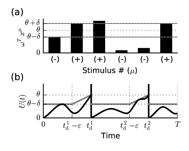
Figure 1: (a) Margin. A neuron receiving static inputs. Inputs from different afferents (elements of $\boldsymbol{x}^{\mu}$) are summed linearly, weighted by the synaptic weights, $\omega_{i}$. The neuron classifies static inputs by comparing the weighted sum of its inputs with a threshold $\theta$. Patterns labeled ‘target’ (+) are required to produce a supra-threshold weighted sum while patterns labeled ‘null’ (-) are required to produce a sub-threshold weighted sum. Here all patterns are classified correctly with a finite margin $\delta$. The optimal solution is defined as the maximal margin solution. (b) Dynamic margin. A neuron receiving dynamic inputs (elements of $\boldsymbol{x}\left(t\right)$, eq. 1) and emits output spikes whenever $U\left(t\right)$ crosses its threshold. Output spikes are required to occur only at $t_{\mathrm{d}}^{1}$ and $t_{\mathrm{d}}^{2}$. The neuron follows the required dynamics, however since the threshold must be reached at the desired times, the margin is by definition zero. The dynamic margin’s temporal profile ($\theta-\mu\left(t\right)$, gray line) allows $U\left(t\right)$ to be close to the threshold near the desired crossing times while remaining far from it at other times, thus endowing $\boldsymbol{\omega}$ with a finite dynamic margin, $\delta$. We define the maximal dynamic margin solution as optimal. In both (a) and (b) we assume $\left\|\boldsymbol{\omega}\right\|=1$.

In static classification systems, it is common to define an optimal weight vector by requiring that, in addition to fulfilling the desired classification of trained examples, the weight vector should obey a large-margin optimality criterion [1]. The margin of each weight vector is the minimal difference between the potential generated by the input examples and the decision threshold, where the difference is measured in units of the norm of the weight vector, $\left\|\boldsymbol{\omega}\right\|$ [Fig. 1(a)]. The optimal solution is then defined as the weight vector with the largest possible margin. SVMs provide an efficient learning algorithm for finding large margin linear classifiers. Furthermore, using the Kernel method, SVMs allow extension of these algorithms to nonlinear classification problems.

This approach cannot be applied straightforwardly to spiking neurons. In the model we consider, $U\left(t\right)$ must approach the threshold $\theta$ continuously at $t_{\mathrm{d}}$. Therefore, the minimum over time of the difference between $U(t)$ and the threshold is, necessarily, zero [Fig. 1(b)]. Thus, the strong temporal correlations in the inputs invalidate the conventional requirement of large margins in SVMs.

Here, we offer an optimality criterion which is appropriate for neural networks and other continuous-time threshold crossing systems. Our criterion is based on constructing dynamic margins: For a given task and a solution weight vector the dynamic margin, $\delta$, is defined as

$$\delta=\min_{t\neq t_{\mathrm{d}}}\frac{-\left(U(t)-\theta\right)}{\left\|\boldsymbol{\omega}\right\|\mu\left(t\right)}\ ,$$ (2)

where $\mu(t)$ is a fixed temporal profile that approaches zero smoothly with a finite slope at $t_{\mathrm{d}}$ and increases monotonically to $1$ away from $t_{\mathrm{d}}$. Thus, qualitatively, solutions with large dynamic margins have potentials which, away from $t_{\mathrm{d}}$, are far away from threshold, and, close to $t_{\mathrm{d}}$, approach the threshold with large slopes. There is a considerable freedom in specifying the detailed shape of the temporal profile $\mu\left(t\right)$, and different choices may be appropriate for different circumstances. Importantly, for any given task and choice of $\mu\left(t\right)$, every solution posses a dynamic margin $\delta>0$ [S. Methods]. As a concrete example, we adopt here the simple form: $\mu\left(t\right)=1$ for $t\leq t_{\mathrm{d}}-\varepsilon$ and $\mu\left(t\right)=\left(t_{\mathrm{d}}-t\right)/\varepsilon$ for $t_{\mathrm{d}}-\varepsilon<t\leq t_{\mathrm{d}}$ where $t_{\mathrm{d}}$ is the first desired time after time $t$ [See gray line in Fig. 1(b)]. For this choice, a dynamic margin $\delta$ implies that for all $t\notin\left[t_{\mathrm{d}}-\varepsilon,t_{\mathrm{d}}\right]$, -$\left(U\left(t\right)-\theta\right)/\left\|\boldsymbol{\omega}\right\|\geq\delta$ and, for all $t_{\mathrm{d}}$, $\left[\mathrm{d}U\left(t_{\mathrm{d}}\right)/\mathrm{d}t\right]/\left\|\boldsymbol{\omega}\right\|\geq\delta/\varepsilon$. The parameter $\varepsilon>0$ represents a tolerance time window prior to $t_{\mathrm{d}}$, within which the voltage $U\left(t\right)$ approaches and reaches the threshold [Fig. 1(b)].

Analogous to static large margin systems, the optimal solution, $\boldsymbol{\omega}^{\star}$ is defined, as the weight vector that possesses the maximal dynamic margin, $\delta^{\star}$, out of all possible solutions, $\boldsymbol{\omega}$. Indeed, we show later that maximizing $\delta$ increases the robustness of solutions to noise in the inputs, justifying the present definition of the optimal weight vector.

Maximizing the Dynamic Margin

We now develop the temporal SVM framework for finding the optimal solution for spiking neurons based on the dynamic margin. Following SVM theory [1] we choose a weight vector magnitude (and threshold value) so that $\left\|\boldsymbol{\omega}\right\|\delta=1$. Thus, maximizing the dynamic margin is equivalent to minimizing the norm of $\boldsymbol{\omega}$ under the constraints (c.I) $U\left(t_{\mathrm{d}}\right)=\theta$ and (c.II) $\frac{\mathrm{d}U}{\mathrm{d}t}\left(t_{\mathrm{d}}\right)\geq-\frac{\mathrm{d}\mu}{\mathrm{d}t}\left(t_{\mathrm{d}}\right)$, (c.III) $-\left(U\left(t\right)-\theta\right)\geq\mu\left(t\right)$ for all $t\neq t_{\mathrm{d}}$,

We apply the Karush-Kuhn-Tucker theorem [7] to show that, despite the continuous nature of the inputs and constraints, the optimal solution can be expressed as a linear sum of a small set of select input vectors [S. Methods],

$$\boldsymbol{\omega}^{\star} = \sum_{t_{\mathrm{d}}}\beta_{t_{\mathrm{d}}}\boldsymbol{x}\left(t_{\mathrm{d}}\right)+\sum_{t_{\mathrm{d}}}\gamma_{t_{\mathrm{d}}}\frac{\mathrm{d}\boldsymbol{x}}{\mathrm{d}t}\left(t_{\mathrm{d}}\right)$$

$$- \sum_{t_{SV}}\alpha_{t_{\mathrm{SV}}}\boldsymbol{x}\left(t_{\mathrm{SV}}\right)$$

This set includes (i) the input vectors at some or all the desired spike times, $\boldsymbol{x}\left(t_{\mathrm{d}}\right)$ imposing the threshold reaching at these times. The associated Lagrange multipliers $\beta_{d}$, can assume any real value although usually it is non-negative. (ii) the input time derivative at some or all the desired times $\frac{\mathrm{d}\boldsymbol{x}}{\mathrm{d}t}\left(t_{\mathrm{d}}\right)$, imposing the inequality on the slope of the potential at threshold; the associated coefficients are $\gamma_{t_{\mathrm{d}}}\geq 0$ and (iii) input patterns, $\boldsymbol{x}\left(t_{\mathrm{SV}}\right)$, at a discrete, problem specific, set of (non-spiking) times, $\left\{t_{\mathrm{SV}}\right\}$, imposing the requirement that the potential remain subthreshold at all non-spiking times. We term this set of vectors as the Support Vectors (SV) of the optimal solution and their associated coefficients $\alpha_{t_{\mathrm{SV}}}>0$ as the SV coefficients. Notably, the support vectors times, $\left\{t_{\mathrm{SV}}\right\}$, are located only at isolated maxima of $U\left(t\right)+\mu\left(t\right)$.

This representation of the optimal solution allows for using well known SVM quadratic programming techniques to evaluate the coefficients $\alpha_{t_{\mathrm{SV}}}$, $\beta_{t_{\mathrm{d}}}$ and $\gamma_{t_{\mathrm{d}}}$ [8, 9, 10, 11]. We have developed an efficient bootstrap algorithm for finding these coefficients and the set of SV times, $\left\{t_{\mathrm{SV}}\right\}$. This algorithm converges asymptotically to the optimal solution [Methods].

Properties of T-SVM Solutions

To demonstrate the application of the T-SVM framework to spiking neurons, we first consider the task of training the LIF neuron to spike at desired times chosen randomly with Poisson statistics with rate $r_{\mathrm{out}}$ in response to randomly chosen input spike patterns with rates $r_{\mathrm{in}}$ [Methods]. Typical solutions to this task, found without dynamic margin maximization [1], possess very small dynamic margins [see example in Fig. 2(a)]. In contrast, the dynamic margin of the optimal solution, $\delta^{\star}$, is of the order of the threshold [Fig. 2(b)]. As predicted, the SV times are located at a set of discrete time points corresponding to maxima of $U\left(t\right)+\mu\left(t\right)$ where $U\left(t\right)$ touches the temporal profile of the dynamic margin, $\theta-\mu\left(t\right)$ [Fig. 2(c)]. To demonstrate the utility of choosing the optimal solution, we examined its robustness by presenting the neuron after learning, with noisy versions of the trained random input-output transformation. The noise consisted of a random Gaussian jitter with mean zero and variance $\sigma^{2}$ added to the timing of each input spike [Fig. 3(a)]. The neuron’s output for the optimal solution is substantially more robust against these perturbations than the typical (non-optimal) solution [Fig. 3(b)].

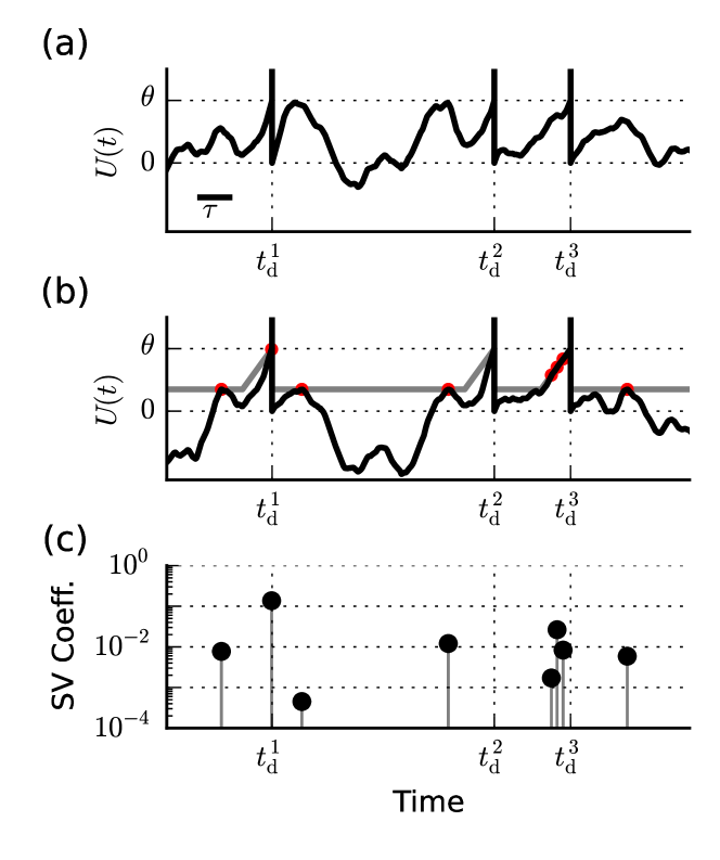
Figure 2: Dynamic margin maximization for spiking neurons. (a)-(b) A segment of the membrane potential traces (black) for different solutions to a single random input-output transformation. (a) depicts a typical solution, found by a Perceptron-like algorithm [1], that possesses a close to zero dynamic margin. The characteristic time scale of the membrane potential dynamics $\tau=\sqrt{\tau_{\mathrm{m}}\tau_{\mathrm{s}}}$ is shown. (b) depicts the optimal solution with the maximal dynamic margin. The temporal profile of the margin, $\theta-\mu\left(t\right)$, is depicted in gray. Red circles depict points at which $U\left(t\right)$ reaches $\theta-\mu\left(t\right)$ (c) The discrete set of support vector coefficients for the optimal solution presented in (b). In (b) and (c) $\varepsilon=\mbox{$\tau$.}$ See Methods for other parameters used.

An important question is how the shape of $\mu\left(t\right)$ affects the properties of the optimal solution. We explore this question by varying the size of the margin temporal window, $\varepsilon$. We find that the mean $\delta^{\star}$ is sensitive to the value of $\varepsilon/\tau$, where $\tau=\sqrt{\tau_{\mathrm{m}}\tau_{\mathrm{s}}}$ is the characteristic correlation time of the inputs; $\delta^{\star}$ approaches zero as $\varepsilon/\tau\rightarrow 0$ and saturates to a finite value for $\varepsilon/\tau\gg 1$ [Fig. 3(c)]. However, despite the increase in dynamic margin for $\varepsilon/\tau\gtrsim 1$, we find that the performance in the presence of noise reaches an optimum at intermediate values, $\varepsilon/\tau\approx 0.3$ [Fig. 3(b), blue line]. This optimum reflects the opposing effects of increasing $\varepsilon$. While increasing $\varepsilon$ increases the margin at times away from the desired spikes, it decreases the minimum allowed slope of the voltage as it crosses threshold at the desired times [Fig. 3(d)]. Thus the optimal value of $\varepsilon/\tau$ represents a tradeoff between the robustness of desired spikes (reflected by the slope at $t_{\mathrm{d}}$) and the distance of the membrane potential from the decision threshold away from $t_{\mathrm{d}}$.

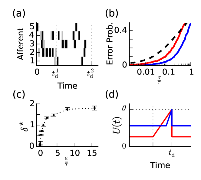
Figure 3: Measuring the solution’s robustness. (a) Following training, the neuron is presented with a jittered version (gray) of the learned patterns (black). (b) Error probability per desired output spike vs. the noise magnitude, $\sigma$, for solutions found without margin maximization (dashed) and with margin maximization ($\varepsilon=\tau$ in red and $\varepsilon=0.3\tau$ in blue with $\tau=\sqrt{\tau_{\mathrm{m}}\tau_{\mathrm{s}}}$). (e) Mean $\delta^{\star}$ vs. tolerance window size. Values are given in units of the mean $\delta^{\star}$ for $\varepsilon=\tau$. Error bars depict one standard error of the mean. (d) Temporal profile of the dynamic margin with the mean $\delta^{\star}$ values found for $\varepsilon=\tau$ (red) and $\varepsilon=0.3\tau$ (blue). See Methods for definition of error and other parameters used.

It is interesting to examine the distribution of $\left\{t_{\mathrm{SV}}\right\}$ relative to $t_{\mathrm{d}}$. For random patterns this distribution mostly reflects the shape of $\mu\left(t\right)$ and the temporal correlation function of the input potentials and post synaptic reset [Fig. 4(a)-(b)]. A high density of SVs just prior to $t_{\mathrm{d}}$ ensures the high slope of $U\left(t\right)$ prior to and at $t_{\mathrm{d}}$. The secondary peak is located exactly at $t_{\mathrm{d}}-\varepsilon$ where the time derivative of $\mu\left(t\right)$ is discontinuous. For tasks with non-random spike patterns, the distribution of SV times is also affected by the spatio-temporal structure of the input spikes and desired output spikes. An example is shown in Figure Fig. 4. Inputs consist of two similar but not identical stimuli, a ‘null’ pattern and a ‘target’ pattern [Methods, Fig. 4(c), red and blue respectively]. The neuron’s task is to remain silent in response to the ‘null’ pattern and fire at the end of the ‘target’ pattern. These patterns are separated by a constant time interval. They repeat at random times and are embedded by a random background Poisson input spikes, making the task of responding to one but not the other input nontrivial. The learning rule finds a large margin solution to this task. The distribution of SV times exhibits a large concentration of SVs immediately after the end of the ‘null’ pattern. These SVs prevent erroneous output spikes in response to this pattern.

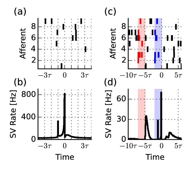
Figure 4: Distribution of SV times. (a) An example of a random input spike train relative to a desired time $t_{\mathrm{d}}$ ($t=0$). Spike times are drawn from independent Poisson processes. (b) Distribution of support vector times relative to $t_{\mathrm{d}}$ for random transformations. (c) Structured input patterns. The neuron is presented with a stream of random Poisson spikes (black) embedded with pairs of repeating stimuli composed of two similar patterns (red and blue). The neuron’s task is to fire only at the end of the blue pattern ($t=0$). (d) Distribution of support vector times relative to the desired time ($t=0$) for the structured input patterns presented in (c). See Methods for other parameters used.

Finally we study how the properties of the maximal dynamic margin solution change with the parameters of the learning task. We find that $\delta^{\star}$ decreases with increasing duration, $T,$ of the learned input-output sequence [Fig. 5(a)]. This is expected since as $T$ increases the weight vector must satisfy an increasing number of constraints. In fact, $\delta^{\star}$ approaches zero at a critical value of $T$, denoting the maximal capacity, beyond which the desired input-output transformation cannot be implemented by an LIF neuron. In addition to the capacity, we are able to analytically calculate [S. Methods] the maximal dynamic margin and the number of support vectors per unit time [Fig. 5(a)-(b)]. Importantly, the number of SVs per unit time does not increase with the number of input spikes as $r_{\mathrm{in}}$ or $N$ increase [Fig. 5(c)]. This demonstrates that a finite number of SVs per synapse is sufficient even when time is continuous and the total rate of input spikes tends to infinity. For example, for intermidated loads and $r_{\mathrm{out}}\tau=0.05,$ the mean number of support vectors is approximatly 0.25 SV’s per time $\tau$. For a neuron with, $\tau\sim 10\mathrm{msec}$, and $r_{\mathrm{out}}\sim 5\mathrm{Hz}$ this implys about 25 support vectors per 1 sec. of learned input-output transformation independent of $N$, $T$ and $r_{\mathrm{in}}$.

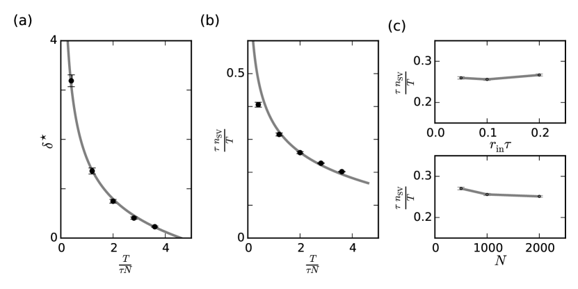
Figure 5: (a) Mean maximal dynamic margin, $\delta^{\star}$, vs. learned pattern duration, $T$. $\delta^{\star}$ is shown in units of the standard deviation of $x_{i}\left(t\right)$. (b) Mean number of SVs per unit time vs. learned pattern duration, $T$. In (a) and (b) black error bars depict simulation data while gray lines depict the approximated theoretical predictions. (c) Mean number of support vectors per unit time vs. mean number of input spikes in time $\tau$ for constant $N=1000$ (top) and vs. $N$ for constant $r_{\mathrm{in}}\tau=0.1$ (bottom). In all panels $\varepsilon=\mbox{$\tau$, $\tau=0.01\sec$},$ $r_{\mathrm{out}}\tau=0.05,\ \tau_{\mathrm{m}}/\tau_{\mathrm{s}}=4$. In (a) and (b) $N=1000,$ $r_{\mathrm{in}}\tau=0.05$. In (c) $T/\tau N=2$.

Nonlinear Computation Using the Kernel Method

Many interesting tasks require nonlinear summation of inputs. Our approach can be extended to include such nonlinearities. To do so, we first note that when the optimal weights, Eq. Maximizing the Dynamic Margin, are substituted, the linear potential can be written as

$$\boldsymbol{\omega}^{T}\boldsymbol{x}\left(t\right)=\sum_{\ell}a^{\ell}\mathcal{K}\left(\boldsymbol{x}^{\ell},\boldsymbol{x}\left(t\right)\right)\ ,$$ (4)

where, $\mathcal{K}\left(\boldsymbol{x}^{\ell},\boldsymbol{x}\left(t\right)\right)=\boldsymbol{x}^{\ell T}\boldsymbol{x}\left(t\right)$ and for the optimal weights, $\left\{\boldsymbol{x}^{\ell}\right\}$ is the set of training vectors $\left\{\boldsymbol{x}\left(t_{\mathrm{d}}\right),\frac{\mathrm{d}\boldsymbol{x}}{\mathrm{d}t}\left(t_{\mathrm{d}}\right),\boldsymbol{x}\left(t_{\mathrm{SV}}\right)\right\}$ and the coefficients $a^{\ell}$ are the corresponding Lagrange coefficients (see (Maximizing the Dynamic Margin)). Extending the linear potential to the non-linear case, we assume that the membrane potential has the from

$$U\left(t\right)=\sum_{l}a^{\ell}\mathcal{K}\left(\boldsymbol{x}^{\ell},\boldsymbol{x}\left(t\right)\right)-\theta x_{\mathrm{reset}}\left(t\right)\ ,$$ (5)

where $a^{\ell}$ and the $N$-dimensional vectors, $\boldsymbol{x}^{\ell}$, are adjustable parameters and $\mathcal{K}\left(\boldsymbol{v},\boldsymbol{u}\right)$ is a nonlinear symmetric positive definite kernel [1]. An example is a polynomial kernel $\mathcal{K}\left(\boldsymbol{v},\boldsymbol{u}\right)=(\boldsymbol{v}^{T}\boldsymbol{u})^{d}$ generalizing the linear case $d=1$ . As before, for a training input $\boldsymbol{x}\left(t\right)$, and desired threshold crossing times, $\left\{t_{\mathrm{d}}\right\}$, $U\left(t\right)$ is required to reach threshold at and only at $t_{\mathrm{d}}$. For a fixed kernel form, the goal of learning is to determine the appropriate ‘template inputs’, $\boldsymbol{x}^{\ell}$, and coefficients $a^{\ell}$. Similar to the kernel extension of SVM, the T-SVM optimization can be extended to the nonlinear case [S. Methods]. The resulting optimal solutions are such that the $a^{\ell}$ coefficients correspond to the Lagrange multiplier coefficients and optimal ‘template inputs’, $\boldsymbol{x}^{\ell}$, correspond to $\left\{\boldsymbol{x}\left(t_{\mathrm{d}}\right),\boldsymbol{x}\left(t_{\mathrm{SV}}\right)\right\}$ where $t_{\mathrm{SV}}$ are a set of non-spiking times (In the nonlinear case we do not explicitly use the time derivatives of the input vectors, see S. Methods for details).

We apply the nonlinear T-SVM to a temporal variant of the XOR problem, a hallmark of nonlinear computation [Fig. 6]. A spiking neuron receives inputs from afferents that fire a single spike during a trial. The neuron has to fire at a time $\Delta$ after the firing of any of its inputs, provided that no additional input arrived during the delay period [Fig. 6(a)]. Thus, the salient feature that the neuron must be tuned to is an inter-spike-interval larger than $\Delta$ in the sequence of incoming spikes. This task cannot be performed by a linear summation of inputs since each input spike, in isolation, must be able to elicit an output spike, whereas the proximal firing of two afferents must leave the neuron subthreshold. Using T-SVM learning we show that a neuron with two input afferents and a quadratic kernel, $\mathcal{K}\left(\boldsymbol{v},\boldsymbol{u}\right)=(\boldsymbol{v}^{T}\boldsymbol{u})^{2}$, can implement the task [Fig. 6(c)-(d)]. In this case, the optimal solution can be expressed by 3 simple template input vectors, $\boldsymbol{x}^{1}=\left(1,0\right)$, $\boldsymbol{x}^{2}=\left(0,1\right)$ and $\boldsymbol{x}^{3}=\left(1,1\right)$. The coefficients for $x^{1}$ and $\boldsymbol{x}^{2}$ are positive and guarantee that each input spike in isolation drives the neuron to fire [Fig. 6(b), (c)]. The negative SV coefficients associated with $\boldsymbol{x}^{3}$ guarantee that an additional incoming spike prior to $\Delta$ interacts nonlinearly with the first spike, curtailing the threshold crossing of $U\left(t\right)$ [Fig. 6(b), (d)].

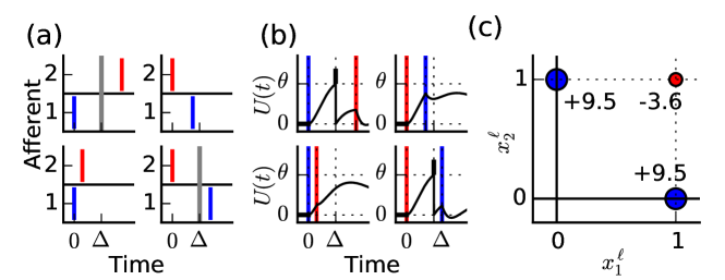
Figure 6: Non Linear Temporal Computation (a) The neuron receives a single spike from each of its two afferents at times $t_{1}$ and $t_{2}$. The neuron is required to fire at a time $\Delta$ after the first input ($t=0)$ if $\left|t_{1}-t_{2}\right|>\Delta$ (top left and bottom right, gray line) and remain silent if $\left|t_{1}-t_{2}\right|<\Delta$ (bottom left and top right). A neuron with a quadratic kernel, $\mathcal{K}\left(\boldsymbol{v},\boldsymbol{u}\right)=\left(\boldsymbol{v}^{T}\boldsymbol{u}\right)^{2}$, is trained with 9 patterns with $t_{1}-t_{2}$ in the range of $\pm 1.25\Delta$. (b) Response of trained neuron to ‘target’ patterns (top left and bottom right) and ‘null’ patterns (bottom left and top right). Blue and red lines depict the input spikes times $t_{1}$ and $t_{2}$ respectively. As required the neuron emits an output spike at time $\Delta$ in the target patterns and remains silent in the null patterns. (c) Circles depict the resulting ‘template inputs’, $\boldsymbol{x}^{\ell}$, and their corresponding coefficients for the optimal solution. The size of the circles is proportional to the coefficient’s value. The resulting subthreshold potential is given by $U_{\mathrm{sub}}(t)=9.5\left(x_{1}(t)^{2}+x_{2}(t)^{2}\right)-3.6\left(x_{1}(t)+x_{2}(t)\right)^{2}$.

A New Framework for Dendritic Computation

The nonlinearities of synaptic integration in the dendritic trees of many neuron types are well established [5, 6]. However, their role in neural information processing is still an open question. According to one proposal [12, 13], the dendritic morphology endow pyramidal cells with a functional ‘two-layer’ Perceptron architecture, in which each nonlinear dendritic branch acts like a sigmoidal unit in the hidden layer of the multi-layer Perceptron. Here we propose that neurons may be able to utilize dendritic nonlinearities to perform nonlinear computation in the spatio-temporal domain by emulating T-SVM with nonlinear kernels. Specifically, the nonlinear synaptic potential, (5), can be interpreted as a weighted sum of contributions from individual dendritic branches. For a kernel of the form $\mathcal{K}\left(\boldsymbol{v},\boldsymbol{u}\right)=f\left(\boldsymbol{v}^{T}\boldsymbol{u}\right),$ the function $f$ may represent the dendritic nonlinearity and the components of the vectors $\boldsymbol{x}\left(t_{\mathrm{d}}\right)$ , and $\boldsymbol{x}\left(t_{\mathrm{SV}}\right)$ can be interpreted as the efficacies of the synapses that innervate the corresponding dendrite. The inputs from different dendrites are then summed linearly at the soma with the SV coefficients representing the coupling strength between a dendrite and the soma [Fig. 7(a)]. Interestingly, emulating T-SVM with the simple quadratic kernel implies that the contribution from each dendritic branch is either excitatory or inhibitory. Higher order kernels allow for mixing of excitatory and inhibitory inputs on the same dendrite.

To demonstrate the dendritic interpretation of kernel T-SVM, we consider a task in which the same sensory inputs should elicit different responses based on some contextual information. Consider, for example, a neuron that receives inputs from two groups of neurons representing stimulus and context respectively. In contextual state $C.A$ the neuron is required to respond to stimuli $S.1$ and $S.2$ with given sets of desired output spike times respectively. In context $C.B$ the desired responses are interchanged. Thus, for the desired output times the neuron must perform an XOR like operation which cannot be implemented in a linear architecture. To understand how this computation can be accomplished with a dendritic tree structure we analyze the simple case where the context dependent response task consists of a single desired output spike [Fig. 7(b)-(c)]. Using a quadratic kernel, $\mathcal{K}\left(\boldsymbol{v},\boldsymbol{u}\right)=\left(\boldsymbol{v}^{T}\boldsymbol{u}\right)^{2}$, the T-SVM algorithm can find a robust solution for this task [Fig. 7(c), top]. In this example 25 stimulus afferents and 25 context afferents impinge on a postsynaptic neuron. 17 dendritic branches analog to 17 Lagrange coefficients and their associated input templates, are sufficient to approximate the optimal solution with 99% accuracy [Fig. 7(b)], contribution from other Lagrange coefficients is negligable. The nonlinear computation relevant for each output spike is distributed onto different sets of dendrites. Specifically, two pairs of dendrites yields the most significant contributions to the total membrane potential [Fig. 7(b)]. However the total activity of one pair (dendrites 1-2) is modulated only in response to pattern $S.1\ C.A$ while the total activity of the other pair (dendrites 3-4) is modulated in response to pattern $S.2\ C.B$ [Fig. 7(c), bottom]. Thus each pair implements a logical AND operation and their output is summed linearly at the soma. It is interesting to note that the scale of activation of individual dendrites is much greater then the scale of the membrane potential itself (compare the vertical scales of top and bottom in Fig. 7(c)). Thus, similar to balanced networks [14, 15], the neuron’s net membrane potential results from the fluctuations in the large excitatory and inhibitory components that largely cancel each other. When more then one desired output spike is learned, the solution structure is more complex: we find some excitatory dendrites without a corresponding inhibitory dendrite, and that desired spikes may be implemented by more then one dendrite pair.

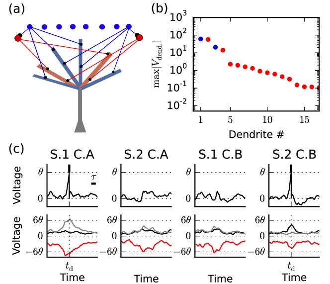
Figure 7: Neuronal architecture for implementing temporal nonlinear kernels. (a) Input afferents (blue circles) project both excitatory (blue) and inhibitory (red), connections onto the neuron’s dendritic tree. Inhibitory inputs from each input afferent may be implemented via feed forward inhibition (red circles). Each input afferent potentially innervates multiple dendritic branches. Inputs are continuously summed nonlinearly within each branch implementing the nonlinear kernel ($\mathcal{K}$ in eq. 5). The contribution from each branch is linearly summed in the neuron’s soma. (b) Maximal contribution of each dendrite to the membrane potential of a neuron with non linear dendrites implementing T-SVM with a quadratic kernel trained on a context dependent respone task (see text). For a quadtaic kernel each dendrite receives exclusively excitatory (blue) or inhibitory (red) input. Dendrites are sorted according to their maximal contribution and the first 17 dendritic branches contribute 99% of the total membrane potential. (c) Top: Voltage traces of the trained neuron. As required, the neuron responds to stimulus $S.1$ with one spike at time $t_{\mathrm{d}}$ and remain silent in response to stimulus $S.2$, while in context $C.A$ and interchanges its responses while in context $C.B$. Bottom: Traces depict the summed voltage contribution of the two first dendrites pairs (see (b)) in black and gray respectively, and the summed contribution of the remaining dendrites (red). The output spike is driven by dendrites 1 and 2 for pattern $S.1\ C.A$, and by dendrites 3 and 4 for pattern $S.2\ C.B$. The pair (1,2) implements a non-linear AND operation for patterns $S.1$ and $C.A$ while the pair (3,4) implements an AND operation for the patterns $S.2$ and $C.B$. The total contribution of the other dendrites is largely non-selctive inhibition; however it is important for shaping the precisely timed response of the neuron. See Methods for parameters used.

Discussion

Supervised learning in spiking networks has been the subject of several recent studies (for a review see [16]). In a previous work [1] we have developed a Perceptron like synaptic learning algorithm for a neuron that is trained to generate a sequence of spikes in given times. While the algorithm converges to a solution when there is one, it does not in general finds a particularly robust solution or one with good generalization abilities. Furthermore, this learning rule does not generalize to tasks requiring nonlinear summation of synaptic inputs.

Here we develop learning rules for finding the optimal weight vectors for spiking neurons extending the theory of large margin systems. Large margin systems and in particular Support Vector Machines have been attractive model systems in Machine and Statistical Learning, due to the robustness of their output, the good generalization capabilities, and the existence of efficient learning algorithms for both the linear and nonlinear systems. This motivates the question whether spiking neuronal circuits can realize similar functionalities. A basic difficulty is the fact that the potential of a spiking neuron approaches the spiking threshold smoothly, implying that the difference between the potential and the decision boundary (the analog of margin in static systems) approaches zero as the neuron fires. To solve this problem we have introduced the new concept of dynamic margin, Importantly, the dynamic margin takes into account the temporal correlations of the system’s dynamics. The application of dynamic margin maximization and the T-SVM framework is not limited to spiking neuron models and can be generalized to any dynamical system in which output is based on threshold crossing [S. Methods]. It allows for robust threshold crossings at desired times while maintaining a large gap between the system’s state variable (membrane potential in the case of neurons) and the decision threshold at other times. Despite the continuous time dynamics, the synaptic weight vector maximizing the dynamic margin can be described using a finite set of parameters, associated with the inputs at the desired output spike times and select times during quiescence; these parameters are analogous to the support vector representation of large margin solutions in static Machine Learning systems. The number of required parameters is proportional to the total duration of the required temporal output spike trains. Indeed, we have shown that the solution with the maximal dynamic margin enjoys greater robustness to input noise. In this work, we have adopted a simple piecewise linear form of the temporal shape of the profile $\mu(t)$ underlying the definition of the dynamic margin, 25. It would be interesting to explore the properties of other temporal profiles and determine how the margin, the robustness to noise, and generalization abilities are affected by the choice of $\mu(t)$. Second, it would be interesting to extend the theory and algorithms to the more biologically relevant case, where the desired times are specified only up to some preassigned precision [1]. Finally, the theory should be extended to allow finding minimal error solutions for cases where the desired input-output transformation is not implementable.

Importantly, we extended the learning capabilities of our spiking neuron model to nonlinear computations by generalizing the kernel method of Support Vector Machines to dynamical threshold crossing systems. We have demonstrated that kernels with relatively simple quadratic nonlinearities are sufficient to perform nonlinear tasks such as temporal and spatial XOR computations and context dependent responses. Indeed quadratic nonlinearities have been shown to account for the nonlinear operation of motion sensing neurons and Complex Cells in visual cortex [17, 18, 19].

In the present work, we have assumed that learning works by modifying the synaptic (linear and nonlinear) efficacies, whereas the temporal integration of synaptic inputs was assumed fixed. However, the T-SVM framework can be extended to more general adaptive dynamical systems in which the temporal filtering of the inputs is adjustable and can be optimized by learning [see example in S. Methods]. Using the kernel method, this extension can be generalized to neurons with nonlinear spatio-temporal kernels allowing for nonlinear interactions between different spatial components of the input and inputs at different times. We leave the investigation of these models and their biological interpretation for future work.

We have proposed that the underlying kernel nonlinearities are implemented in biological circuits by the nonlinear synaptic integration of dendritic branches. Our proposed function for dendritic nonlinearities share similarity with the pioneering work of Mel et al. [12, 13, 20]. The difference between the two proposed functional architectures is similar to the difference between a two layer perceptron and that of a Kernel SVMs. The advantage of the latter is the existence of an efficient learning algorithm that is guaranteed to converge to the (optimal) solution provided that such a solution exists. In the present context, our proposal differs from earlier models in that it takes into account explicitly the dynamic nature of the decision making of spiking neuron, whereas the multilayer perceptron model is a rate based, largely static input-output system. Furthermore, using the SV representation, our proposal provides insight into the contributions of the different dendrites to the performance of the task, by encoding in their synapses specific template input vectors representing the stream of training inputs during spiking and nonspiking times. Such interpretation is lacking for solutions derived by generic gradient based approaches to learning in a two-layer perceptron and the dendritic architectures that mimic them. Nevertheless, the two-layer perceptron model is advantageous to our model in certain aspects. In particular, in our SVM model, to allow for successful learning, each presynaptic source should be in general allowed to innervate all branches; whereas the input architecture can be restricted in learning the two-layer perceptron model. Further studies of learning in neuron models with realistic morphologies learning to perform interesting computations are needed in order to shed further light on the important question of the functional role of the extensive nonlinearities and morphologies of neurons’ dendritic trees. Finally, the learning algorithms presented here are designed to find and reveal the properties of optimal weight vectors of trained spiking neurons. At present, SVM like learning algorithms, as the one presented here are not a plausible model of the biological process of learning. Implementing large margin solutions of these algorithms by a neurally plausible online learning algorithm remains an important open challenge for computational neuroscience.

Methods

T-SVM Algorithm: Here we describe the algorithm used to find the maximal dynamic margin solution. The algorithm consists of two iterative stages: Sampling stage and Optimization Stage. In the sampling stage we construct a discrete set of times (and corresponding input patterns) on which optimization should be performed. In the optimization stage we use quadratic programing algorithms to find the optimal value of $\theta$ and the Lagrange multipliers.

The algorithm is as follows:

1. Initialization: Choose a set of sampled times $\left\{t_{\mathrm{SV}}\right\}$ arbitrarily.

2. Optimization: Maximize the dynamic margin using only the current set $\left\{t_{\mathrm{SV}}\right\}$ by using a quadratic programing algorithm.

3. Sampling

   1. Present all the input patterns to the neuron using the neuron’s dynamics and the current set of parameters.

   2. Construct a set of new sampled times, $\left\{t_{\mathrm{new}\text{ }}\right\}$ consisting of the times of the maximal value of $U$$\left(t\right)+\mu\left(t\right)$ in every time segment in which $U\left(t\right)>\theta-\mu\left(t\right)$.

   3. For every $t_{\mathrm{new}}\notin\left\{t_{\mathrm{SV}}\right\}$ add $t_{\mathrm{new}}$ to the set $\left\{t_{\mathrm{SV}}\right\}$. $t_{\mathrm{new}}$ is considered to be in $\left\{t_{\mathrm{SV}}\right\}$ if $\exists t_{\mathrm{SV}}:\ \left|t_{\mathrm{SV}}-t_{\mathrm{new}}\right|<\epsilon_{t}$ where $\epsilon_{t}$ is an arbitrarily small time constant.

4. Stopping Criteria: If no new times were added to $\left\{t_{\mathrm{SV}}\right\}$, stop.

5. Return to step 2.

For any $\epsilon_{t}>0$ this algorithm samples at most $T/\epsilon_{t}$ points in time. Thus for any $\epsilon_{t}>0$ the algorithm will converge in a finite number of iterations. For $\epsilon_{t}\rightarrow 0$ this algorithm will asymptotically converge to the optimal solution.

Desired outputs for random patterns: To avoid pathologies, output spikes are not allowed between $t=0$ and $t=\tau_{\mathrm{m}}$. For $t\in\left(\tau_{\mathrm{m}},T\right)$ spikes are drawn from a Poisson process with rate $r_{\mathrm{out}}/\left(1-\frac{\tau_{\mathrm{m}}}{T}\right)$.

Definition of error due to jitter: We observed that the mean inaccuracy of desired spikes in error free time segments is small compared to $\tau$ and approximately proportional to the standard deviation of the jitter (not shown). Thus, we define the neuron’s output in the $n$’th desired spike time, $t_{\mathrm{d}}^{n}$, as erroneous if the number of output spikes in $\left[\left(t_{\mathrm{d}}^{n-1}+t_{\mathrm{d}}^{n}\right)/2,\ \left(t_{\mathrm{d}}^{n}+t_{\mathrm{d}}^{n+1}\right)/2\right]$ is different form one.

Parameters used: Figure 2: $N=1000,\ r_{\mathrm{in}}\tau=0.14,\ r_{\mathrm{out}}\tau=0.07,\ \tau=\sqrt{\tau_{\mathrm{m}}\tau_{\mathrm{s}}}=14\mathrm{msec,\ }\tau_{\mathrm{m}}/\tau_{\mathrm{s}}=8,\ T/\tau N=1.4\,$. Figure 3: In (b) and (c) $N=1000,\ r_{\mathrm{in}}=10\mathrm{Hz},$ $r_{\mathrm{out}}=5\,\mathrm{Hz},\ \tau=10\,\mathrm{msec},\ \tau_{\mathrm{m}}=20$ msec, $T=12\,\mathrm{sec}$. Figure 4: In all panels $\tau=14\,\mathrm{msec},\ \tau_{\mathrm{m}}=40\,\mathrm{msec},\ \varepsilon=\mbox{$\tau$},\ T/N\tau=2,\ N=1000$. In (a)-(b) $r_{\mathrm{in}}=10\mathrm{Hz}.$ In (c)-(d) $r_{\mathrm{in}}=20\mathrm{Hz}$, ‘target’ pattern consist of Poisson input spikes of duration $2\tau$. ‘null’ pattern is the ‘target’ patern were 10% of the spikes were randomly modified. Figure 6: $\tau_{\mathrm{m}}=10\mbox{msec}$, $\tau_{\mathrm{s}}=5\mathrm{msec}$, $\varepsilon=5\mathrm{msec}$, $\Delta=5\mathrm{msec}$. Figure 7: $N=50$, $T=0.5\mathrm{sec}$, $r_{\mathrm{in}}=20\mathrm{Hz}$, $\tau_{\mathrm{m}}=20\mbox{msec}$, $\tau_{\mathrm{s}}=5\mathrm{msec}$, $\varepsilon=10\mathrm{msec}$.

Supplementary Methods: Temporal Support Vectors for Spiking Neural Networks

1 Existence of Positive Dynamic Margin

In this section we will show that for any $\boldsymbol{\omega}$ which satisfies the requirements of the task the dynamic margin is always strictly positive given that $\boldsymbol{x}\left(t\right)$ and $\mu\left(t\right)$ are well behaved (see below).

Theorem: Given the inputs $\boldsymbol{x}\left(t\right)$, desired times $\left\{t_{\mathrm{d}}\right\}$, profile of the dynamic margin $\mu\left(t\right)$, weight vector $\boldsymbol{\omega}$ and the following:

1. $\boldsymbol{\omega}$ is a solution, i.e. for all $t_{\mathrm{d}}\in\left\{t_{\mathrm{d}}\right\}$, $U\left(t_{\mathrm{d}}\right)=\theta,$ $\frac{\mathrm{d}U}{\mathrm{d}t}\left(t_{\mathrm{d}}\right)>0$ and $U\left(t\right)<\theta$ for all $t\neq t_{\mathrm{d}}$.

2. $U\left(t\right)$ and $\mu\left(t\right)$ are continuous between $t_{\mathrm{d}}$’s

3. $\mu\left(t\right)>0$ for $t\neq t_{\mathrm{d}}$, $\mu\left(t_{\mathrm{d}}\right)=0$, $\frac{\mathrm{d}\mu}{\mathrm{d}t}\left(t_{\mathrm{d}}\right)>-\infty$, $\max_{t}\mu\left(t\right)=1$.

Then the dynamic margin, $\delta$, is greater then zero.

Proof: From the definition of the dynamic margin of a given solution, $\boldsymbol{\omega}$ (Eq. 2 in the main text), we have that $\theta-U\left(t\right)\geq\left\|\boldsymbol{\omega}\right\|\delta\mu\left(t\right)$, where $\delta$ is the maximal constant for which this inequality is satisfied for all $t\neq t_{\mathrm{d}}$. To show that $\delta>0$ we will bound it from below using a constant $\epsilon>0$ that satisfies

$$\theta-U\left(t\right)\geq\epsilon\mu\left(t\right)$$ (6)

for all $t$. This ensures that $\delta\geq\frac{\epsilon}{\left\|\boldsymbol{\omega}\right\|}>0$.

For every $t_{\mathrm{d}}$ we define,

$$\epsilon_{t_{\mathrm{d}}}\equiv\min_{t}\frac{\theta-U\left(t\right)}{t_{\mathrm{d}}-t}/\max_{t}\frac{\mu\left(t\right)}{t_{\mathrm{d}}-t}$$ (7)

where the minimum and maximum are taken over $t\in\left(t_{\mathrm{d}}-\Delta_{t_{\mathrm{d}}},t_{\mathrm{d}}\right)$ with some $\Delta_{t_{\mathrm{d}}}>0$ smaller then the inter-spike-interval between $t_{\mathrm{d}}$ and the desired time before it. Both the nominator and the denominator are positive and the denominator is finite. Thus $\epsilon_{t_{\mathrm{d}}}>0$.

In addition we have

$$\frac{\theta-U\left(t\right)}{t_{\mathrm{d}}-t} \geq\min_{t^{\prime}}\frac{\theta-U\left(t^{\prime}\right)}{t_{\mathrm{d}}-t^{\prime}}$$ (8)

$$\frac{\mu\left(t\right)}{t_{\mathrm{d}}-t} \leq\max_{t^{\prime}}\frac{\mu\left(t^{\prime}\right)}{t_{\mathrm{d}}-t^{\prime}}$$ (9)

Multiplying both sides of (9) by $\epsilon_{t_{\mathrm{d}}}$ we find that for all $t\in\left(t_{\mathrm{d}}-\Delta_{t_{\mathrm{d}}},t_{\mathrm{d}}\right)$,

$$\theta-U\left(t\right)\geq\epsilon_{t_{\mathrm{d}}}\mu\left(t\right)\ .$$ (10)

We define

$$\epsilon_{1}=\min_{t_{\mathrm{d}}}\epsilon_{t_{\mathrm{d}}}\ .$$ (11)

Now, for every $t\notin\bigcup_{t_{\mathrm{d}}}\left(t_{\mathrm{d}}-\Delta_{t_{\mathrm{d}}},t_{\mathrm{d}}\right]$ we have $U\left(t\right)<\theta$ therefore there exists $\epsilon_{2}>0$ such that for these times:

$$\theta-U\left(t\right)\geq\epsilon_{2}\geq\epsilon_{2}\mu\left(t\right)$$ (12)

since $\mu$$\left(t\right)>0$ and the maximal value of $\mu\left(t\right)$ is set to $1$.

Finally we define:

$$\epsilon=\min\left(\epsilon_{1},\epsilon_{2}\right)>0\ ,$$ (13)

and we have that for all times $t$

$$\theta-U\left(t\right)\geq\epsilon\mu\left(t\right)\ _{\blacksquare}$$ (14)

2 Maximizing the Dynamic Margin

To maximize the dynamic margin we minimize $\frac{1}{2}\boldsymbol{\omega}^{T}\boldsymbol{\omega}$ under the constraints (c.I) $-\left(U\left(t\right)-\theta\right)\geq\mu\left(t\right)$ for all $t\neq t_{\mathrm{d}}$, (c.II) $U\left(t_{\mathrm{d}}\right)=\theta$ and (c.III) $\frac{\mathrm{d}U}{\mathrm{d}t}\left(t_{\mathrm{d}}\right)\geq-\frac{\mathrm{d}\mu}{\mathrm{d}t}\left(t_{\mathrm{d}}\right)$. We define the Lagrangian:

$$\mathcal{L}=\frac{1}{2}\boldsymbol{\omega}^{T}\boldsymbol{\omega}-\int_{0}^{T}\mathrm{dt}\alpha\left(t\right)\left[-\left(U\left(t\right)-\theta\right)-\mu\left(t\right)\right]-\sum_{t_{\mathrm{d}}}\gamma_{t_{\mathrm{d}}}\left[\frac{\mathrm{d}U}{\mathrm{d}t}\left(t_{\mathrm{d}}\right)+\frac{\mathrm{d}\mu}{\mathrm{d}t}\left(t_{\mathrm{d}}\right)\right]-\sum_{t_{\mathrm{d}}}\beta_{t_{\mathrm{d}}}\left[U\left(t_{\mathrm{d}}\right)-\theta\right]\ ,$$ (15)

and our task is to minimize $\mathcal{L}$ w.r.t. $\boldsymbol{\omega}$ and $\theta$, and maximize $\mathcal{L}$ w.r.t. $\alpha\left(t\right)$, $\beta_{t_{\mathrm{d}}}$ and $\gamma_{t_{\mathrm{d}}}$ under the constraints: $\alpha\left(t\right)\geq 0$ and $\gamma_{t_{\mathrm{d}}}\geq 0$. The Karush-Kuhn-Tucker theorem states that, for the optimal values of the coefficients, constraints (c.I)-c.(III) are satisfied and the following hold:

$$\forall t\neq t_{\mathrm{d}}\ \alpha\left(t\right)\left[-\left(U\left(t\right)-\theta\right)-\mu\left(t\right)\right] = 0$$ (16)

$$\alpha\left(t\right) \geq 0$$

$$\forall t_{\mathrm{d}}\ \gamma_{t_{\mathrm{d}}}\left[\frac{\mathrm{d}U}{\mathrm{d}t}\left(t_{\mathrm{d}}\right)+\frac{\mathrm{d}\mu}{\mathrm{d}t}\left(t_{\mathrm{d}}\right)\right] = 0$$

$$\gamma_{t_{\mathrm{d}}} \geq 0$$

That is $\alpha\left(t\right)$ and $\gamma_{t_{\mathrm{d}}}$ can be non zero only at times in which the constraints (c.I) and (c.III) respectively are satisfied with an equality. We assume that for a generic $U\left(t\right)$ and $\mu\left(t\right)$ the analytical shape of $U\left(t\right)+\mu\left(t\right)$ does not allow for a constant value for any non infinitesimal duration. Thus, it follows that $\alpha\left(t\right)$ can be non-zero only at isolated local maxima of $U\left(t\right)+\mu\left(t\right)$ in which $U\left(t\right)=\theta-\mu\left(t\right)$. $\alpha\left(t\right)$ can be written as

$$\alpha\left(t\right)=\sum_{t_{\mathrm{SV}}}\alpha_{t_{\mathrm{SV}}}\delta\left(t-t_{\mathrm{SV}}\right)$$ (17)

where $\delta\left(t\right)$ is the Dirac delta function.

Taking the derivative of $\mathcal{L}$ w.r.t. $\boldsymbol{\omega}^{T}$ and equating to zero, together with (17) leads to the form of the optimal weight vector $\boldsymbol{\omega}^{\star}$ given by eq. 3 in the main text.

It is important to note that despite the fact that constraints (c.I) and (c.II) implicitly enforce constraint (c.III), we find that explicitly including (c.III) in $\mathcal{L}$ is required for the application of the Karush-Kuhn-Tucker theorem for this case. In fact, without including the slope constraints in $\mathcal{L}$, it is possible to construct simple examples in which the solution cannot be expressed with $\alpha\left(t\right)$ in the form of (17).

3 Effective Perceptron Theory for the Dynamic Margin and Support Vectors

The capacity of the LIF neuron to realize random input-output transformations and its dependance on the various parameters was studied extensively, numerically and analytically, in [1]. It was found that the relevant time constant of the neuronal dynamics is $\tau=\sqrt{\tau_{\mathrm{m}}\tau_{\mathrm{s}}}$ and that the duration of the longest implementable input-output transformation, $T_{c}$, is extensive and that $T_{c}/N\tau$ only depends on the mean number of desired output spike within time $\tau$, $r_{\mathrm{out}}\tau$. In addition, for $r_{\mathrm{out}}\tau\lesssim 0.1$, the system is well approximated by an effective Perceptron (see below). This allows for the evaluation of the capacity and of statistical properties of the solutions below the capacity, using the Gardner theory of the Perceptron [2]. Further, the above analogy with the Perceptron can also be used to investigate the change in $\delta^{\star}$ and the properties of the SV’s as the load, i.e., the duration of the spike sequence, $T$, increases. The predicted mean $\delta^{\star}$ and mean number of SV’s, as well as the numerical simulations are shown in Figure 5(a)-(b).

Effective Perceptron Approximation (Gardner Theory): We approximate the spiking neuron as an effective Perceptron with $N_{\mathrm{eff}}=N-r_{\mathrm{out}}T$ input synapses, classifying $P_{\mathrm{eff}}=T\left(1/\tau+r_{\mathrm{out}}\right)$ uncorrelated patterns, $r_{\mathrm{out}}T$ patterns labeled as ‘target‘ patterns and $T/\tau$ patterns labeled as ‘null‘ patterns. The capacity, mean margin, and mean number of support vectors, $n_{\mathrm{SV}}$, are a function of the effective load $\alpha_{\mathrm{eff}}=\frac{P_{\mathrm{eff}}}{N_{\mathrm{eff}}}$, and the ratio between the effective number of ‘target‘ patterns and $P_{\mathrm{eff}}$, $f_{\mathrm{eff}}=r_{\mathrm{out}}\tau/\left(1+r_{\mathrm{out}}\tau\right)$. In practice we derive expressions for $\alpha_{\mathrm{eff}}$ and $n_{\mathrm{SV}}$ as a function of the margin in units of the standard deviation of the inputs, $\kappa=\frac{\delta^{\star}}{\mathrm{std}\left(x_{i}\left(t\right)\right)}$ and $f_{\mathrm{eff}}$:

$$\alpha_{\mathrm{eff}}\left(\kappa,f_{\mathrm{eff}}\right) =\left[f_{\mathrm{eff}}\int_{\eta-\kappa}^{\infty}Dt\left(t-\eta+\kappa\right)^{2}+\left(1-f_{\mathrm{eff}}\right)\int_{-\eta-\kappa}^{\infty}Dt\left(t+\eta+\kappa\right)^{2}\right]^{-1}$$ (18)

$$n_{\mathrm{SV}}\left(\kappa,f_{\mathrm{eff}}\right) =P_{\mathrm{eff}}\left[f_{\mathrm{eff}}H\left(\eta-\kappa\right)+\left(1-f_{\mathrm{eff}}\right)H\left(-\eta-\kappa\right)\right]$$ (19)

where $Dt=\frac{e^{-\frac{t^{2}}{2}}}{\sqrt{2\pi}}\mathrm{d}t$, $H\left(y\right)=\int_{y}^{\infty}Dt$, and $\eta$ is given by the solution to

$$f_{\mathrm{eff}}\int_{\eta-\kappa}^{\infty}Dt\left(t-\eta+\kappa\right)=\left(1-f_{\mathrm{eff}}\right)\int_{-\eta-\kappa}^{\infty}Dt\left(t+\eta+\kappa\right)\ .$$ (20)

Simple algebra can be used to then find the relation between $\delta^{\star}$, $\mbox{$\tau$}n_{\mathrm{SV}}/T$ and $T/\tau N$.

4 Dual Lagrangian and Application of Kernel Method for T-SVM

To apply the Kernel method to T-SVM we enforce the slope constraints (c.III) implicitly by excluding from the temporal integration in (15) segments of duration $\Delta$ prior to every $t_{\mathrm{d}}$ and removing the Lagrange coefficients enforcing the slope constraints, $\left\{\gamma_{t_{\mathrm{d}}}\right\}$. In this case, the K.K.T theorem implies that the optimal value of $\alpha\left(t\right)$ satisfies equations (16) and (17) where $t\in\left\{t_{\mathrm{SV}}\right\}$ only if $t$ is an isolated local maxima of $U\left(t\right)+\mu\left(t\right)$ in which $U\left(t\right)=\theta-\mu\left(t\right)$ or if $t=t_{\mathrm{d}}-\Delta$. In the $\Delta\rightarrow 0$ limit this exclusion is equivalent to explicitly enforcing constraints (c.III). In practice our simulation of nonlinear kernels are approximated with discrete time steps of size $\Delta t$, and we use $\Delta=\Delta t$.

To apply the kernel method we derive the dual Lagrangian. Since our algorithm uses a sequence of sets of sampled times we consider the primal Lagrangian for a given set $\left\{t_{s}\right\}$ and a set of desired times $\left\{t_{\mathrm{d}}\right\}$ :

$$\mathcal{L}=\frac{1}{2}\boldsymbol{\omega}^{T}\boldsymbol{\omega}-\sum_{t_{s}}\alpha_{t_{s}}\left[-\left(U\left(t_{s}\right)-\theta\right)-\mu\left(t_{s}\right)\right]-\sum_{t_{\mathrm{d}}}\beta_{t_{\mathrm{d}}}\left[U\left(t_{\mathrm{d}}\right)-\theta\right]\ .$$ (21)

The dual Lagrangian is obtained by minimizing $\mathcal{L}$ w.r.t. $\boldsymbol{\omega}^{T}$ and expressing the Lagrangian using the optimal weight vector:

$$\mathcal{Q}= -\frac{1}{2}\sum_{t_{s},t_{s}^{\prime}}\alpha_{t_{s}}K\left[\boldsymbol{x}\left(t_{s}\right),\boldsymbol{x}\left(t_{s}^{\prime}\right)\right]\alpha_{t_{s}^{\prime}}-\frac{1}{2}\sum_{t_{\mathrm{d}},t_{\mathrm{d}}^{\prime}}\beta_{t_{\mathrm{d}}}K\left[\boldsymbol{x}\left(t_{\mathrm{d}}\right),\boldsymbol{x}\left(t_{\mathrm{d}}^{\prime}\right)\right]\beta_{t_{\mathrm{d}}^{\prime}}$$ (22)

$$-\sum_{t_{s},t_{\mathrm{d}}}\alpha_{t_{s}}K\left[\boldsymbol{x}\left(t_{s}\right),\boldsymbol{x}\left(t_{\mathrm{d}}\right)\right]\beta_{t_{\mathrm{d}}}+\sum_{t_{s}}\alpha_{t_{s}}\mu\left(t_{s}\right)$$

$$+\theta\left[\beta_{t_{\mathrm{d}}}\left(1+x_{\mathrm{reset}}\left(t_{\mathrm{d}}\right)\right)-\sum_{t_{s}}\alpha_{t_{s}}\left(1+x_{\mathbb{\mathrm{reset}}}\left(t_{s}\right)\right)\right]$$

where $K\left[\boldsymbol{u},\boldsymbol{v}\right]=\boldsymbol{u}^{T}\boldsymbol{v}$. To solve the optimization problem we maximize $\mathcal{Q}$ w.r.t $\alpha_{t_{s}}$ and $\beta_{t_{\mathrm{d}}}$ under the constraints:

$$\alpha_{t_{s}} \geq 0$$ (23)

$$\beta_{t_{\mathrm{d}}}\left(1+x_{\mathrm{reset}}\left(t_{\mathrm{d}}\right)\right)-\sum_{t_{s}}\alpha_{t_{s}}\left(1+x_{\mathbb{\mathrm{reset}}}\left(t_{s}\right)\right) =0$$

In practice, $\beta_{t_{\mathrm{d}}}$ and $\theta$ can be found analytically and SVM optimization can be performed only w.r.t the $\alpha_{t_{s}}$ coefficients.

For nonlinear kernels one simply replaces the linear kernel $K\left[\boldsymbol{u},\boldsymbol{v}\right]$ in $\mathcal{Q}$, with a nonlinear, symmetric, positive definite kernel $\mathcal{K}\left[\boldsymbol{u},\boldsymbol{v}\right]$.

5 Extensions

5.1 Dynamic Margin for Non-Spiking Dynamical Systems

The application of T-SVM is not limited to spiking neurons only. Dynamic margin maximization can be applied to any dynamical system in which decision is based on threshold crossing.

We consider a binary dynamical unit, whose output, $s\left(t\right)$, is given by $s\left(t\right)=\mathrm{sign}\left(U\left(t\right)-\theta\right),$ where $\theta$ and $U\left(t\right)$ are the units threshold and internal dynamical variable analog to the membrane potential in the spiking neurons, respectively. The unit linearly sums $N$ input afferents defined by $N$ time varying signals, $x_{i}\left(t\right),\ i=1,2,\dots,N$. For a set of weights, $\omega_{i},\ i=1,2,\dots,N$, $U\left(t\right)$ is defined by

$$U\left(t\right) = \boldsymbol{\omega}^{T}\boldsymbol{x}\left(t\right)\ ,$$ (24)

where $\boldsymbol{\omega}$ and $\boldsymbol{x}\left(t\right)$ are the $N$-dimensional vectors of the weights and inputs at time $t$, respectively.

The training data consists of an input trace vector, $\boldsymbol{x}\left(t\right)$, and a desired output function, $y\left(t\right)=\pm 1$ which is assumed to be piece-wise constant, for all $t\in\left[0,T\right]$. $y\left(t\right)$ defines a discrete set of desired threshold crossing times, $\left\{t_{\mathrm{d}}\right\}$, at which $y\left(t\right)$ changes sign. The task of learning is to modify $\boldsymbol{\omega}$ such that the unit’s output equals the desired output, i.e., $s\left(t\right)=y\left(t\right)$ for all $t\neq t_{\mathrm{d}}$. Thus, $U\left(t\right)$ is required to be above $\theta$ when $y\left(t\right)=1$, below $\theta$ when $y\left(t\right)=-1$ and cross $\theta$ precisely at the desired times, $\left\{t_{\mathrm{d}}\right\}$.

As in the case of spiking neurons, simple margin maximization cannot be applied to these kind of systems due to the continuous threshold crossing at $t_{\mathrm{d}}$. However it is possible to generalize the definition of the dynamic margin for this case. The dynamic margin of a weight vector is defined as:

$$\delta=\min_{t\neq t_{\mathrm{d}}}\frac{y\left(t\right)\left(U(t)-\theta\right)}{\left\|\boldsymbol{\omega}\right\|\mu\left(t\right)}\ ,$$ (25)

where here we require that $\mu(t)$ is a continuous function that satisfies: $\mu\left(t\right)>0$ for $t\neq t_{\mathrm{d}}$, $\mu\left(t_{\mathrm{d}}\right)=0$, $\frac{\mathrm{d}\mu}{\mathrm{d}t}\left(t_{\mathrm{d}}^{-}\right)>-\infty$, $\frac{\mathrm{d}\mu}{\mathrm{d}t}\left(t_{\mathrm{d}}^{+}\right)<\infty$ and $\max_{t}\mu\left(t\right)=1$. As before, we define the optimal solution, $\boldsymbol{\omega}^{\star}$, as the weight vector that possesses the maximal dynamic margin, $\delta^{\star}$.

Maximizing the dynamic margin in this case is equivalent to minimizing the norm of $\boldsymbol{\omega}$ under the constraints (c.I) $y\left(t\right)\left(U\left(t\right)-\theta\right)\geq\mu\left(t\right)$ for all $t\neq t_{\mathrm{d}}$; (c.II) $U\left(t_{\mathrm{d}}\right)=\theta$; (c.III) $y\left(t_{\mathrm{d}}^{-}\right)\frac{\mathrm{d}U}{\mathrm{d}t}\left(t_{\mathrm{d}}^{-}\right)\leq\frac{\mathrm{d}\mu}{\mathrm{d}t}\left(t_{\mathrm{d}}^{-}\right)$ and (c.IV) $y\left(t_{\mathrm{d}}^{+}\right)\frac{\mathrm{d}U}{\mathrm{d}t}\left(t_{\mathrm{d}}^{+}\right)\geq\frac{\mathrm{d}\mu}{\mathrm{d}t}\left(t_{\mathrm{d}}^{+}\right)$. Note that for continuous inputs, imposing (c.I) fulfills all the requirements of the task and implicitly enforces the remaining constraints. However as in the spiking neurons case, for the application of the K.K.T theorem constraints (c.II)-(c.IV) must be explicitly included in the optimization as explained above. T-SVM algorithm, and the Kernel method can be applied to these type of systems in a similar manner as to spiking neurons.

5.2 Learning Optimal Temporal Filters

An example of system in which optimal temporal filters can be learned such is

$$U\left(t\right)=\int_{0}^{\tau_{\max}}\mathrm{d}\tau\boldsymbol{\omega}\left(\tau\right)^{T}\boldsymbol{x}\left(t-\tau\right)\ .$$ (26)

where $\boldsymbol{\omega_{i}}\left(\tau\right)$ is the synaptic temporal filter of the $i-$th afferent. In this case we define the dynamic margin according to (25) with $\left\|\boldsymbol{\omega}\right\|=\left[\int_{0}^{\tau_{\max}}\mathrm{d}\tau\boldsymbol{\omega}\left(\tau\right)^{T}\boldsymbol{\omega}\left(\tau\right)\right]^{\frac{1}{2}}$, and maximizing it can be done in the same manner as before. The optimal solution $\boldsymbol{\omega}\left(\tau\right)$ is a sum of a set of select input traces: $\boldsymbol{x}\left(t_{\mathrm{d}}-\tau\right)$, $\frac{\mathrm{d}\boldsymbol{x}}{\mathrm{d}t}\left(t_{\mathrm{d}}-\tau\right)$ , and $\boldsymbol{x}\left(t_{\mathrm{SV}}-\tau\right)$ and with coefficients $\beta_{t_{\mathrm{d}}}$, $-\gamma_{t_{\mathrm{d}}}y\left(t_{\mathrm{\mathring{d}}}^{-}\right),$ and $\alpha_{t_{\mathrm{SV}}}y\left(t_{\mathrm{SV}}\right)$, respectively.

References

- [1] Vapnik V. The nature of statistical learning theory. springer; 2000.
- [2] Rosenblatt F. Principles of neurodynamics: Perceptrons and the theory of brain mechanisms. Spartan Books, Washington, DC; 1962.
- [3] Minsky ML, Papert SA. Perceptrons: expanded edition. MIT Press Cambridge, MA, USA; 1988.
- [4] Memmesheimer RM, Rubin R, Ölveczky BP, Sompolinsky H. Learning Precisely Timed Spikes. Neuron. 2014;82(4):925–938.
- [5] London M, Häusser M. Dendritic Computation. Annual Review of Neuroscience. 2005;28(1):503–532. doi:10.1146/annurev.neuro.28.061604.135703.
- [6] Major G, Larkum ME, Schiller J. Active Properties of Neocortical Pyramidal Neuron Dendrites. Annual Review of Neuroscience. 2013;36(1):1–24. doi:10.1146/annurev-neuro-062111-150343.
- [7] Kuhn HW, Tucker AW. Nonlinear programming. In: Proceedings of the Second Berkeley Symposium on Mathematical Statistics and Probability, 1950. University of California Press, Berkeley and Los Angeles; 1951. p. 481–492.
- [8] Anlauf JK, Biehl M. The AdaTron: An Adaptive Perceptron Algorithm. EPL (Europhysics Letters). 1989;10(7):687.
- [9] Nocedal J, Wright S. Numerical Optimization. Springer Series in Operations Research and Financial Engineering. Springer New York; 2006.
- [10] Laskov P, Gehl C, Krüger S, Müller KR. Incremental support vector learning: Analysis, implementation and applications. The Journal of Machine Learning Research. 2006;7:1909–1936.
- [11] Karasuyama M, Takeuchi I. Multiple incremental decremental learning of support vector machines; 2009. p. 907–915.
- [12] Poirazi P, Mel BW. Impact of active dendrites and structural plasticity on the memory capacity of neural tissue. Neuron. 2001;29(3):779–796.
- [13] Polsky A, Mel BW, Schiller J. Computational subunits in thin dendrites of pyramidal cells. Nature Neuroscience. 2004;7(6):621–627.
- [14] van Vreeswijk C, Sompolinsky H. Chaos in neuronal networks with balanced excitatory and inhibitory activity. Science. 1996;274(5293):1724–1726.
- [15] Vreeswijk C, Sompolinsky H. Chaotic balanced state in a model of cortical circuits. Neural computation. 1998;10(6):1321–1371.
- [16] Gutig R. To spike, or when to spike? Current opinion in neurobiology. 2014;25:134–139.
- [17] Hassenstein B, Reichardt W. Systemtheoretische analyse der zeit-, reihenfolgen-und vorzeichenauswertung bei der bewegungsperzeption des rüsselkäfers chlorophanus. Zeitschrift für Naturforschung B. 1956;11(9-10):513–524.
- [18] Adelson EH, Bergen JR. Spatiotemporal energy models for the perception of motion. JOSA A. 1985;2(2):284–299.
- [19] Emerson RC, Bergen JR, Adelson EH. Directionally selective complex cells and the computation of motion energy in cat visual cortex. Vision research. 1992;32(2):203–218.
- [20] Jadi MP, Behabadi BF, Poleg-Polsky A, Schiller J, Mel BW. An Augmented Two-Layer Model Captures Nonlinear Analog Spatial Integration Effects in Pyramidal Neuron Dendrites. Proceedings of the IEEE. 2014;102(5):782–798. doi:10.1109/JPROC.2014.2312671.

References

- [1] Memmesheimer RM, Rubin R, Ölveczky BP, Sompolinsky H. Learning Precisely Timed Spikes. Neuron. 2014;82(4):925–938.
- [2] Gardner E. The space of interactions in neural network models. J Phys A: Math Gen. 1988;21(1):257. doi:10.1088/0305-4470/21/1/030.