Reinforcement Learning for Branch-and-Bound Optimisation
using Retrospective Trajectories

Abstract

Combinatorial optimisation problems framed as mixed integer linear programmes (MILPs) are ubiquitous across a range of real-world applications. The canonical branch-and-bound algorithm seeks to exactly solve MILPs by constructing a search tree of increasingly constrained sub-problems. In practice, its solving time performance is dependent on heuristics, such as the choice of the next variable to constrain (‘branching’). Recently, machine learning (ML) has emerged as a promising paradigm for branching. However, prior works have struggled to apply reinforcement learning (RL), citing sparse rewards, difficult exploration, and partial observability as significant challenges. Instead, leading ML methodologies resort to approximating high quality handcrafted heuristics with imitation learning (IL), which precludes the discovery of novel policies and requires expensive data labelling. In this work, we propose retro branching; a simple yet effective approach to RL for branching. By retrospectively deconstructing the search tree into multiple paths each contained within a sub-tree, we enable the agent to learn from shorter trajectories with more predictable next states. In experiments on four combinatorial tasks, our approach enables learning-to-branch without any expert guidance or pre-training. We outperform the current state-of-the-art RL branching algorithm by $3$-$5\times$ and come within $20\%$ of the best IL method’s performance on MILPs with $500$ constraints and $1000$ variables, with ablations verifying that our retrospectively constructed trajectories are essential to achieving these results.

1 Introduction

A plethora of real-world problems fall under the broad category of co (vehicle routing and scheduling (Korte and Vygen 2012); protein folding (Perdomo-Ortiz et al. 2012); fundamental science (Barahona 1982)). Many co problems can be formulated as milp whose task is to assign discrete values to a set of decision variables, subject to a mix of linear and integrality constraints, such that some objective function is maximised or minimised. The most popular method for finding exact solutions to milp is bnb (Land and Doig 1960); a collection of heuristics which increasingly tighten the bounds in which an optimal solution can reside (see Section 3). Among the most important of these heuristics is variable selection or branching (which variable to use to partition the chosen node’s search space), which is key to determining bnb solve efficiency (Achterberg and Wunderling 2013).

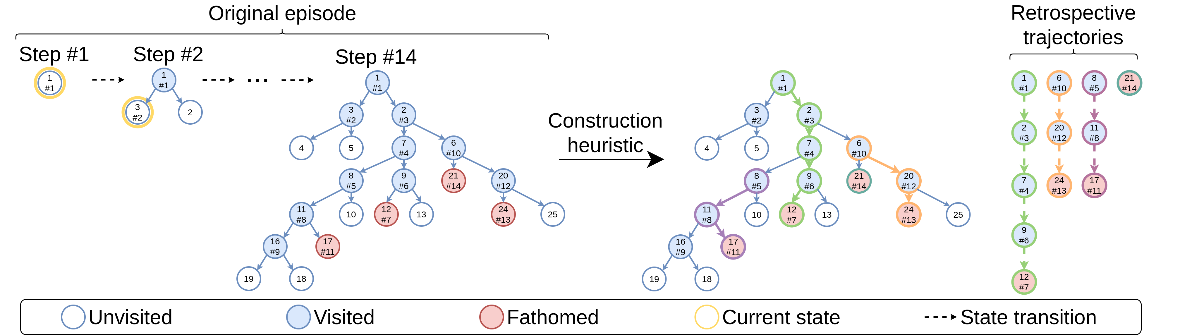
Figure 1: The proposed retro branching approach used during training. Each node is labelled with: Top: The unique ID assigned when it was added to the tree, and (where applicable); bottom: The step number (preceded by a ‘#’) at which it was visited by the brancher in the original mdp. The milp is first solved with the brancher and the bnb tree stored as usual (forming the ‘original episode’). Then, ignoring any nodes never visited by the agent, the nodes are added to trajectories using some ‘construction heuristic’ (see Sections 4 and 6) until each eligible node has been added to one, and only one, trajectory. Crucially, the order of the sequential states within a given trajectory may differ from the state visitation order of the original episode, but all states within the trajectory will be within the same sub-tree. These trajectories are then used for training.

sota learning-to-branch approaches typically use the il paradigm to predict the action of a high quality but computationally expensive human-designed branching expert (Gasse et al. 2019). Since branching can be formulated as a mdp (He, Daumé, and Eisner 2014), rl seems a natural approach. The long-term motivations of rl include the promise of learning novel policies from scratch without the need for expensive expert data, the potential to exceed expert performance without human design, and the capability to maximise the performance of a policy parameterised by an expressivity-constrained dnn.

However, branching has thus far proved largely intractable for rl for reasons we summarise into three key challenges. (1) Long episodes: Whilst even random branching policies are theoretically guaranteed to eventually find the optimal solution, poor decisions can result in episodes of tens of thousands of steps for the $500$ constraint $1000$ variable milp considered by Gasse et al. 2019. This raises the familiar rl challenges of reward sparsity (Trott et al. 2019), credit assignment (Harutyunyan et al. 2019), and high variance returns (Mao et al. 2019). (2) Large state-action spaces: Each branching step might have hundreds or thousands of potential branching candidates with a huge number of unique possible sub-milp states. Efficient exploration to discover improved trajectories in such large state-action spaces is a well-known difficulty for rl (Agostinelli et al. 2019; Ecoffet et al. 2021). (3) Partial observability: When a branching decision is made, the next state given to the brancher is determined by the next sub-milp visited by the node selection policy. Jumping around the bnb tree without the brancher’s control whilst having only partial observability of the full tree makes the future states seen by the agent difficult to predict. Etheve et al. 2020 therefore postulated the benefit of keeping the mdp within a sub-tree to improve observability and introduced the sota fmsts rl branching algorithm. However, in order to achieve this, fmsts had to use a dfs node selection policy which, as we demonstrate in Section 6, is highly sub-optimal and limits scalability.

In this work, we present retro branching; a simple yet effective method to overcome the above challenges and learn to branch via reinforcement. We follow the intuition of Etheve et al. (2020) that constraining each sequential mdp state to be within the same sub-tree will lead to improved observability. However, we posit that a branching policy taking the ‘best’ actions with respect to only the sub-tree in focus can still provide strong overall performance regardless of the node selection policy used. This is aligned with the observation that leading heuristics such as SB and PB also do not explicitly account for the node selection policy or predict how the global bound may change as a result of activity in other sub-trees. Assuming the validity of this hypothesis, we can discard the dfs node selection requirement of fmsts whilst retaining the condition that sequential states seen during training must be within the same sub-tree.

Concretely, our retro branching approach (shown in Figure 1 and elaborated on in Section 4) is to, during training, take the search tree after the bnb instance has been solved and retrospectively select each subsequent state (node) to construct multiple trajectories. Each trajectory consists of sequential nodes within a single sub-tree, allowing the brancher to learn from shorter trajectories with lower return variance and more predictable future states. This approach directly addresses challenges (1) and (3) and, whilst the state-action space is still large, the shorter trajectories implicitly define more immediate auxiliary objectives relative to the tree. This reduces the difficulty of exploration since shorter trajectory returns will have a higher probability of being improved upon via stochastic action sampling than when a single long mdp is considered, thereby addressing (2). Furthermore, retro branching relieves the fmsts requirement that the agent must be trained in a dfs node selection setting, enabling more sophisticated strategies to be used which are better suited for solving larger, more complex milp.

We evaluate our approach on milp with up to $500$ constraints and $1000$ variables, achieving a $3$-$5\times$ improvement over fmsts and coming within $\approx 20\%$ of the performance of the sota il agent of Gasse et al. (2019). Furthermore, we demonstrate that, for small instances, retro branching can uncover policies superior to il; a key motivation of using rl. Our results open the door to the discovery of new branching policies which can scale without the need for labelled data and which could, in principle, exceed the performance of sota handcrafted branching heuristics.

2 Related Work

Since the invention of bnb for exact co by Land and Doig (1960), researchers have sought to design and improve the node selection (tree search), variable selection (branching), primal assignment, and pruning heuristics used by bnb, with comprehensive reviews provided by Achterberg 2007 and Tomazella and Nagano 2020. We focus on branching.

Classical branching heuristics. pb (Benichou et al. 1971) and sb (Applegate et al. 1995, 2007) are two canonical branching algorithms. pb selects variables based on their historic branching success according to metrics such as bound improvement. Although the per-step decisions of pb are computationally fast, it must initialise the variable pseudocosts in some way which, if done poorly, can be particularly damaging to overall performance since early bnb decisions tend to be the most influential. sb, on the other hand, conducts a one-step lookahead for all branching candidates by computing their potential local dual bound gains before selecting the most favourable variable, and thus is able to make high quality decisions during the critical early stages of the search tree’s evolution. Despite its simplicity, sb is still today the best known policy for minimising the overall number of bnb nodes needed to solve the problem instance (a popular bnb quality indicator). However, its computational cost renders sb infeasible in practice.

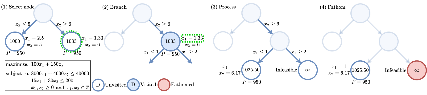
Figure 2: Typical $4$-stage procedure iteratively repeated by bnb to solve an milp. Each node represents an milp derived from the original milp being solved, and each edge represents the constraint added to derive a new child node (sub-milp) from a given parent. Each node is labelled with the decision variable values of the solved LP relaxation on the right hand side, the corresponding dual bound in the centre, and the established primal bound beneath. Each edge is labelled with the introduced constraint to generate the child node. Green dotted outlines are used to indicate which node and variable were selected in stages $(1)$ and $(2)$ to lead to stages $(3)$ and $(4)$. The global primal ($P$) and dual ($D$) bounds are increasingly constrained by repeating stages $1$-$4$ until $P$ and $D$ are equal, at which point a provably optimal solution will have been found. Note that for clarity we only show the detailed information needed at each stage, but that this does not indicate any change to the state of the tree.

Learning-to-branch. Recent advances in deep learning have led ml researchers to contribute to exact co (surveys provided by Lodi and Zarpellon 2017, Bengio, Lodi, and Prouvost 2021, and Cappart et al. 2021). Khalil et al. 2016 pioneered the community’s interest by using il to train a svm to imitate the variable rankings of sb after the first $500$ bnb node visits and thereafter use the svm. Alvarez, Louveaux, and Wehenkel 2017 similarly imitated sb, but learned to predict the sb scores directly using Extremely Randomized Trees (Geurts, Ernst, and Wehenkel 2006). These approaches performed promisingly, but their per-instance training and use of sb at test time limited their scalability.

These issues were overcome by Gasse et al. 2019, who took as input a bipartite graph representation capturing the current bnb node state and predicted the corresponding action chosen by sb using a gcn. This alleviated the reliance on extensive feature engineering, avoided the use of sb at inference time, and demonstrated generalisation to larger instances than seen in training. Works since have sought to extend this method by introducing new observation features to generalise across heterogeneous co instances (Zarpellon et al. 2021) and designing sb-on-a-GPU expert labelling methods for scalability (Nair et al. 2021).

Etheve et al. 2020 proposed fmsts which, to the best of our knowledge, is the only published work to apply rl to branching and is therefore the sota rl branching algorithm. By using a dfs node selection strategy, they used the dqn approach (Mnih et al. 2013) to approximate the Q-function of the bnb sub-tree size rooted at the current node; a local Q-function which, in their setting, was equivalent to the number of global tree nodes. Although fmsts alleviated issues with credit assignment and partial observability, it relied on using the dfs node selection policy (which can be far from optimal), was fundamentally limited by exponential sub-tree sizes produced by larger instances, and its associated models and data sets were not open-accessed.

3 Background

Mixed integer linear programming. An milp is an optimisation task where values must be assigned to a set of $n$ decision variables subject to a set of $m$ linear constraints such that some linear objective function is minimised. milp can be written in the standard form

$$\arg\min_{\mathbb{x}}\big{\{}\mathbb{c}^{\top}\mathbb{x}|\mathbb{A}\mathbb{x}\leq\mathbb{b},\mathbb{l}\leq\mathbb{x}\leq\mathbb{u},\mathbb{x}\in\mathbb{Z}^{p}\times\mathbb{R}^{n-p}\big{\}},$$ (1)

where $\mathbb{c}\in\mathbb{R}^{n}$ is a vector of the objective function’s coefficients for each decision variable in $\mathbb{x}$ such that $\mathbb{c}^{\top}\mathbb{x}$ is the objective value, $\mathbb{A}\in\mathbb{R}^{m\times n}$ is a matrix of the $m$ constraints’ coefficients (rows) applied to $n$ variables (columns), $\mathbb{b}\in\mathbb{R}^{m}$ is the vector of variable constraint right-hand side bound values which must be adhered to, and $\mathbb{l},\mathbb{u}\in\mathbb{R}^{n}$ are the respective lower and upper variable value bounds. milp are hard to solve owing to their integrality constraint(s) whereby $p\leq n$ decision variables must be an integer. If these integrality constraints are relaxed, the milp becomes a lp, which can be solved efficiently using algorithms such as simplex (Nelder and Mead 1965). The most popular approach for solving milp exactly is bnb.

Branch-and-bound. bnb is an algorithm composed of multiple heuristics for solving milp. It uses a search tree where nodes are milp and edges are partition conditions (added constraints) between them. Using a divide and conquer strategy, the milp is iteratively partitioned into sub-milp with smaller solution spaces until an optimal solution (or, if terminated early, a solution with a worst-case optimality gap guarantee) is found. The task of bnb is to evolve the search tree until the provably optimal node is found.

Concretely, as summarised in Figure 2, at each step in the algorithm, bnb: (1) Selects an open (unfathomed leaf) node in the tree whose sub-tree seems promising to evolve; (2) selects (‘branches on’) a variable to tighten the bounds on the sub-milp’s solution space by adding constraints either side of the variable’s lp solution value, generating two child nodes (sub-milp) beneath the focus node; (3) for each child, i) solve the relaxed lp (the dual problem) to get the dual bound (a bound on the best possible objective value in the node’s sub-tree) and, where appropriate, ii) solve the primal problem and find a feasible (but not necessarily optimal) solution satisfying the node’s constraints, thus giving the primal bound (the worst-case feasible objective value in the sub-tree); and (4) fathom any children (i.e. consider the sub-tree rooted at the child ‘fully known’ and therefore excluded from any further exploration) whose relaxed lp solution is integer-feasible, is worse than the incumbent (the globally best feasible node found so far), or which cannot meet the non-integrality constraints of the milp. This process is repeated until the primal-dual gap (global primal-dual bound difference) is $0$, at which point a provably optimal solution to the original milp will have been found.

Note that the heuristics (i.e. primal, branching, and node selection) at each stage jointly determine the performance of bnb. More advanced procedures such as cutting planes (Mitchell 2009) and column generation (Barnhart et al. 1998) are available for enhancement, but are beyond the scope of this work. Note also that solvers such as SCIP 2022 only store ‘visitable’ nodes in memory, therefore in practice fathoming occurs at a feasible node where a branching decision led to the node’s two children being outside the established optimality bounds, being infeasible, or having an integer-feasible dual solution, thereby closing the said node’s sub-tree.

Q-learning. Q-learning is typically applied to sequential decision making problems formulated as an mdp defined by tuple $\{\mathcal{S},\mathcal{U},\mathcal{T},\mathcal{R},\gamma\}$. $\mathcal{S}$ is a finite set of states, $\mathcal{U}$ a set of actions, $\mathcal{T}:\mathcal{S}\times\mathcal{U}\times\mathcal{S}\rightarrow[0,1]$ a transition function from state $s\in\mathcal{S}$ to $s^{\prime}\in\mathcal{S}$ given action $u\in{U}$, $\mathcal{R}:\mathcal{S}\rightarrow\mathbb{R}$ a function returning a scalar reward from $s$, and $\gamma\in[0,1]$ a factor by which to discount expected future returns to their present value. It is an off-policy temporal difference method which aims to learn the action-value function mapping state-action pairs to the expected discounted sum of their immediate and future rewards when following a policy $\pi:\mathcal{S}\rightarrow\mathcal{U}$, $Q^{\pi}(s,u)=\mathbb{E}_{\pi}\big{[}\sum_{t^{\prime}=t+1}^{\infty}\gamma_{t^{\prime}-1}r(s_{t^{\prime}})|s_{t}{=}s,u_{t}{=}u\big{]}$. By definition, an optimal policy $\pi_{*}$ will select an action which maximises the true Q-value $Q_{*}(s,u)$, $\pi_{*}(s)=\arg\max_{u^{\prime}}Q_{*}(s,u^{\prime})$. For scalability, dqn (Mnih et al. 2013; van Hasselt, Guez, and Silver 2015) approximates this true Q-function using a dnn parameterised by $\theta$ such that $Q_{\theta}(s,u)\approx Q_{*}(s,u)$.

4 Retro Branching

We now describe our retro branching approach for learning-to-branch with rl.

States. At each time step $t$ the bnb solver state is comprised of the search tree with past branching decisions, per-node lp solutions, the global incumbent, the currently focused leaf node, and any other solver statistics which might be tracked. To convert this information into a suitable input for the branching agent, we represent the milp of the focus node chosen by the node selector as a bipartite graph. Concretely, the $n$ variables and $m$ constraints are connected by edges denoting which variables each constraint applies to. This formulation closely follows the approach of Gasse et al. 2019, with a full list of input features at each node detailed in Appendix E.

Actions. Given the milp state $s_{t}$ of the current focus node, the branching agent uses a policy $\pi(u_{t}|s_{t})$ to select a variable $u_{t}$ from among the $p$ branching candidates.

Original full episode transitions. In the original full bnb episode, the next node visited is chosen by the node selection policy from amongst any of the open nodes in the tree. This is done independently of the brancher, which observes state information related only to the current focus node and the status of the global bounds. As such, the transitions of the ‘full episode’ are partially observable to the brancher, and it will therefore have the challenging task of needing to aggregate over unobservable states in external sub-trees to predict the long-term values of states and actions.

Retrospectively constructed trajectory transitions (retro branching). To address the partial observability of the full episode, we retrospectively construct multiple trajectories where all sequential states in a given trajectory are within the same sub-tree, and where the trajectory’s terminal state is chosen from amongst the as yet unchosen fathomed sub-tree leaves. A visualisation of our approach is shown in Figure 1. Concretely, during training, we first solve the instance as usual with the rl brancher and any node selection heuristic to form the ‘original episode’. When the instance is solved, rather than simply adding the originally observed mdp’s transitions to the dqn replay buffer, we retrospectively construct multiple trajectory paths through the search tree. This construction process is done by starting at the highest level node not yet added to a trajectory, selecting an as yet unselected fathomed leaf in the sub-tree rooted at said node using some ‘construction heuristic’ (see Section 6), and using this root-leaf pair as a source-destination with which to construct a path (a ‘retrospective trajectory’). This process is iteratively repeated until each eligible node in the original search tree has been added to one, and only one, retrospective trajectory. The transitions of each trajectory are then added to the experience replay buffer for learning. Note that retrospective trajectories are only used during training, therefore retro branching agents have no additional inference-time overhead.

Crucially, retro branching determines the sequence of states in each trajectory (i.e. the transition function of the mdp) such that the next state(s) observed in a given trajectory will always be within the same sub-tree (see Figure 1) regardless of the node selection policy used in the original bnb episode. Our reasoning behind this idea is that the state(s) beneath the current focus node within its sub-tree will have characteristics (bounds, introduced constraints, etc.) which are strongly related with those of the current node, making them more observable than were the next states to be chosen from elsewhere in the search tree, as can occur in the ‘original bnb’ episode. Moreover, by correlating the agent’s maximum trajectory length with the depth of the tree rather than the total number of nodes, reconstructed trajectories have orders of magnitude fewer steps and lower return variance than the original full episode, making learning tractable on large milp. Furthermore, because the sequential nodes visited are chosen retrospectively in each trajectory, unlike with fmsts, any node selection policy can be used during training. As we show in Section 6, this is a significant help when solving large and complex milp.

Rewards. As demonstrated in Section 6, the use of reconstructed trajectories enables a simple distance-to-goal reward function to be used; a $r=-1$ punishment is issued to the agent at each step except when the agent’s action fathomed the sub-tree, where the agent receives $r=0$. This provides an incentive for the the branching agent to reach the terminal state as quickly as possible. When aggregated over all trajectories in a given sub-tree, this auxiliary objective corresponds to fathoming the whole sub-tree (and, by extension, solving the milp) in as few steps as possible. This is because the only nodes which are stored by SCIP 2022 and which the brancher will be presented with will be feasible nodes which potentially contain the optimal solution beneath them. As such, any action chosen by the brancher which provably shows either the optimal solution to not be beneath the current node or which finds an integer feasible dual solution (i.e. an action which fathoms the sub-tree beneath the node) will be beneficial, because it will prevent SCIP from being able to further needlessly explore the node’s sub-tree.

A note on partial observability. In the above retrospective formulation of the branching mdp, the primal, branching, and node selection heuristics active in other sub-trees will still influence the future states and fathoming conditions of a given retrospective trajectory. We posit that there are two extremes; dfs node selection where future states are fully observable to the brancher, and non-dfs node selection where they are heavily obscured. As shown in Section 6, our retrospective node selection setting strikes a balance between these two extremes, attaining sufficient observability to facilitate learning while enabling the benefits of short, low variance trajectories with sophisticated node selection strategies which make handling larger milp tractable.

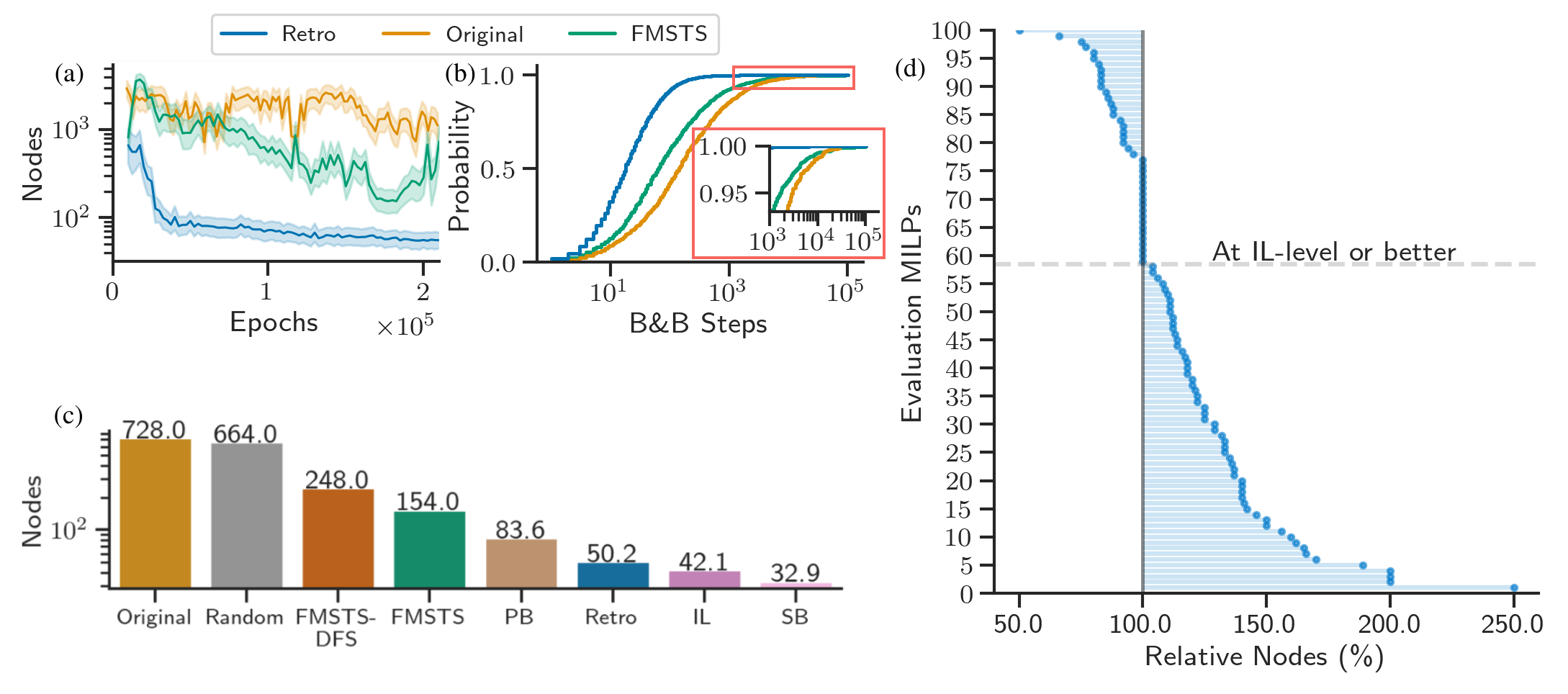
Figure 3: Performances of the branching agents on the $500\times 1000$ set covering instances. (a) Validation curves for the rl agents evaluated in the same non-dfs setting. (b) CDF of the number of bnb steps taken by the rl agents for each instance seen during training. (c) The best validation performances of each branching agent. (d) The instance-level validation performance of the retro branching agent relative to the il agent, with rl matching or beating il on $42\%$ of test instances.

5 Experimental Setup

All code for reproducing the experiments and links to the generated data sets are provided at https://github.com/cwfparsonson/retro_branching.

Network architecture and learning algorithm. We used the gcn architecture of Gasse et al. 2019 to parameterise the dqn value function with some minor modifications which we found to be helpful (see Appendix B.1). We trained our network with n-step DQN (Sutton 1988; Mnih et al. 2013) using prioritised experience replay (Schaul et al. 2016), soft target network updates (Lillicrap et al. 2019), and an epsilon-stochastic exploration policy (see Appendix A.1 for a detailed description of our rl approach and the corresponding algorithms and hyperparameters used).

B&B environment. We used the open-source Ecole (Prouvost et al. 2020) and PySCIPOpt (Maher et al. 2016) libraries with SCIP $7.0.1$ (SCIP 2022) as the backend solver to do instance generation and testing. Where possible, we used the training and testing protocols of Gasse et al. (2019).

MILP Problem classes. In total, we considered four NP-hard problem benchmarks: set covering (Balas, Ho, and Center 2018), combinatorial auction (Leyton-Brown, Pearson, and Shoham 2000), capacitated facility location (Litvinchev and Ozuna Espinosa 2012), and maximum independent set (Bergman et al. 2016).

Baselines. We compared retro branching against the sota fmsts rl algorithm of Etheve et al. (2020) (see Appendix F for implementation details) and the sota il approach of Gasse et al. (2019) trained and validated with $100\,000$ and $20\,000$ strong branching samples respectively. For completeness, we also compared against the sb heuristic imitated by the il agent, the canonical pb heuristic, and a random brancher (equivalent in performance to most infeasible branching (Achterberg, Koch, and Martin 2004)). Note that we have ommited direct comparison to the sota tuned commercial solvers, which we do not claim to be competitive with at this stage. To evaluate the quality of the agents’ branching decisions, we used $100$ validation instances (see Appendix C for an analysis of this data set size) which were unseen during training, reporting the total number of tree nodes and lp iterations as key metrics to be minimised.

6 Results & Discussion

6.1 Performance of Retro Branching

Comparison to the SOTA RL branching heuristics. We considered set covering instances with $500$ rows and $1000$ columns. To demonstrate the benefit of the proposed retro branching method, we trained a baseline ‘Original’ agent on the original full episode, receiving the same reward as our retro branching agent ($-1$ at each non-terminal step and $0$ for a terminal action which ended the episode). We also trained the sota rl fmsts branching agent in a dfs setting and, at test time, validated the agent in both a dfs (‘fmsts-dfs’) and non-dfs (‘fmsts’) environment to fairly compare the policies. Note that the fmsts agent serves as an ablation to analyse the influence of training on retrospective trajectories, since it uses our auxiliary objective but without retrospective trajectories, and that the Original agent further ablates the auxiliary objective since its ‘terminal step’ is defined as ending the bnb episode (where it receives $r_{t}=0$ rather than $r_{t}=-1$). As shown in Figure 3a, the Original agent was unable to learn on these large instances, with retro branching achieving $14\times$ fewer nodes at test time. fmsts also performed poorly, with highly unstable learning and a final performance $5\times$ and $3\times$ poorer than retro branching in the dfs and non-dfs settings respectively (see Figure 3c). We posit that the cause of the poor fmsts performance is due to its use of the sub-optimal dfs node selection policy, which is ill-suited for handling large milp and results in $\approx 10\%$ of episodes seen during training being on the order of 10-100k steps long (see Figure 3b), which makes learning significantly harder for rl.

Comparison to non-RL branching heuristics. Having demonstrated that the proposed retro branching method makes learning-to-branch at scale tractable for rl, we now compare retro branching with the baseline branchers to understand the efficacy of rl in the context of the current literature. Figure 3c shows how retro branching compares to other policies on large $500\times 1000$ set covering instances. While the agent outperforms pb, it only matches or beats il on $42\%$ of the test instances (see Figure 3d) and, on average, has a $\approx 20\%$ larger bnb tree size. Therefore although our rl agent was still improving and was limited by compute (see Appendix A.2), and in spite of our method outperforming the current sota fmsts rl brancher, rl has not yet been able to match or surpass the sota il agent at scale. This will be an interesting area of future work, as discussed in Section 7.

6.2 Analysis of Retro Branching

Verifying that RL can outperform IL. In addition to not needing labelled data, a key motivation for using rl over il for learning-to-branch is the potential to discover superior policies. While Figure 3 showed that, at test-time, retro branching matched or outperformed il on $42\%$ of instances, il still had a lower average tree size. As shown in Table 1, we found that, on small set covering instances with $165$ constraints and $230$ variables, rl could outperform il by $\approx 20\%$. While improvement on problems of this scale is not the primary challenge facing ml-bnb solvers, we are encouraged by this demonstration that it is possible for an rl agent to learn a policy better able to maximise the performance of an expressivity-constrained network than imitating an expert such as sb without the need for pre-training or expensive data labelling procedures (see Appendix H).

For completeness, Table 1 also compares the retro branching agent to the il, pb, and sb branching policies evaluated on $100$ unseen instances of four NP-hard co benchmarks. We considered instances with $10$ items and $50$ bids for combinatorial auction, $5$ customers and facilities for capacitated facility location, and $25$ nodes for maximum independent set. rl achieved a lower number of tree nodes than pb and il on all problems except combinatorial auction. This highlights the potential for rl to learn improved branching policies to solve a variety of milp.

Table 1: Test-time comparison of the best agents on the evaluation instances of the four NP-hard small co problems considered.

	Set Covering		Combinatorial Auction		Capacitated Facility Location		Maximum Independent Set
Method	# LPs	# Nodes	# LPs	# Nodes	# LPs	# Nodes	# LPs	# Nodes
sb	$184$	$6.76$	$13.2$	$4.64$	$28.2$	$10.2$	$19.2$	$3.80$
pb	$258$	$12.8$	$22.0$	$7.80$	$\mathbf{28.0}$	$10.2$	$25.4$	$5.77$
il	$244$	$10.5$	$\mathbf{16.0}$	$\mathbf{5.29}$	$\mathbf{28.0}$	$10.2$	$20.1$	$4.08$
Retro	$\mathbf{206}$	$\mathbf{8.68}$	$18.1$	$5.73$	$28.4$	$\mathbf{10.1}$	$\mathbf{19.1}$	$\mathbf{4.01}$

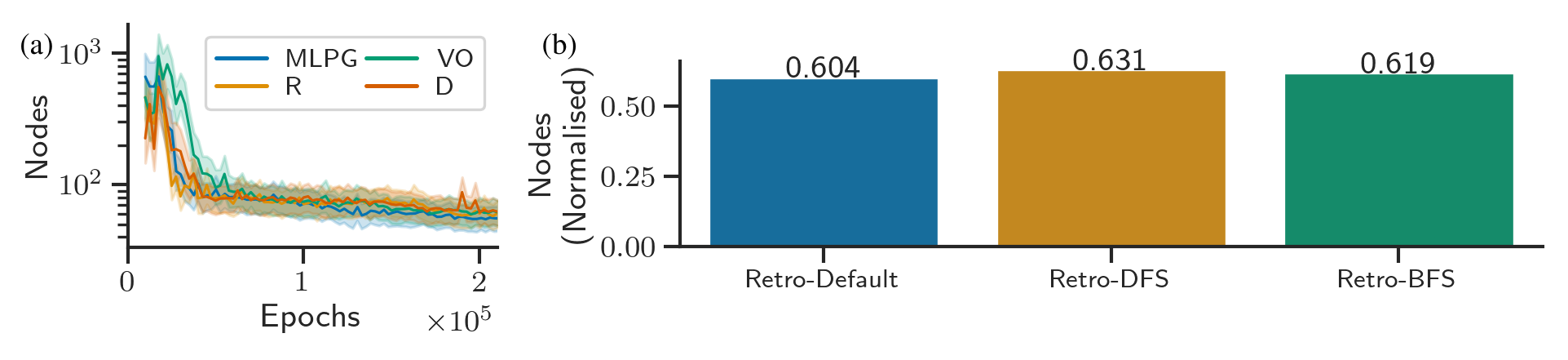
Figure 4: $500\times 1000$ set covering performances. (a) Validation curves for four retro branching agents each trained with a different trajectory construction heuristic: Maximum LP gain (MLPG); random (R); visitation order (VO); and deepest (D). (b) The performances of the best retro branching agent deployed in three different node selection environments (default SCIP, dfs, and bfs) normalised relative to the performances of pb (measured by number of tree nodes).

Demonstrating the independence of retro branching to future state selection. As described in Section 4, in order to retrospectively construct a path through the search tree, a fathomed leaf node must be selected. We refer to the method for selecting the leaf node as the construction heuristic. The future states seen by the agent are therefore determined by the construction heurisitc (used in training) and the node selection heuristic (used in training and inference).

During our experiments, we found that the specific construction heuristic used had little impact on the performance of our agent. Figure 4a shows the validation curves for four agents trained on $500\times 1000$ set covering instances each using one of the following construction heuristics: Maximum LP gain (‘MLPG’: Select the leaf with the largest LP gain); random (‘R’: Randomly select a leaf); visitation order (‘VO’: Select the leaf which was visited first in the original episode); and deepest (‘D’: Select the leaf which results in the longest trajectory). As shown, all construction heuristics resulted in roughly the same performance (with MLPG performing only slightly better). This suggests that the agent learns to reduce the trajectory length regardless of the path chosen by the construction heuristic. Since the specific path chosen is independent of node selection, we posit that the relative strength of an rl agent trained with retro branching will also be independent of the node selection policy used.

To test this, we took our best retro branching agent trained with the default SCIP node selection heuristic and tested it on the $500\times 1000$ validation instances in the default, dfs, and bfs SCIP node selection settings. To make the performances of the brancher comparable across these settings, we normalised the mean tree sizes with those of pb (a branching heuristic independent of the node selector) to get the performance relative to pb in each environment. As shown in Figure 4b, our agent achieved consistent relative performance regardless of the node selection policy used, indicating its indifference to the node selector.

7 Conclusions

We have introduced retro branching; a retrospective approach to constructing bnb trajectories in order to aid learning-to-branch with rl. We posited that retrospective trajectories address the challenges of long episodes, large state-action spaces, and partially observable future states which otherwise make branching an acutely difficult task for rl. We empirically demonstrated that retro branching outperforms the current sota rl method by $3$-$5\times$ and comes within $20\%$ of the performance of il whilst matching or beating it on $42\%$ of test instances. Moreover, we showed that rl can surpass the performance of il on small instances, exemplifying a key advantage of rl in being able to discover novel performance-maximising policies for expressivity-constrained networks without the need for pre-training or expert examples. However, retro branching was not able to exceed the il agent at scale. In this section we outline areas of further work.

Partial observability. A limitation of our proposed approach is the remaining partial observability of the mdp, with activity external to the current sub-tree and branching decision influencing future bounds, states, and rewards. In this and other studies, variable and node selection have been considered in isolation. An interesting approach would be to combine node and variable selection, giving the agent full control over how the bnb tree is evolved.

Reward function. The proposed trajectory reconstruction approach can facilitate a simple rl reward function which would otherwise fail were the original ‘full’ tree episode used. However, assigning a $-1$ reward at each step in a given trajectory ignores the fact that certain actions, particularly early on in the bnb process, can have significant influence over the length of multiple trajectories. This could be accounted for in the reward signal, perhaps by using a retrospective backpropagation method (similar to value backpropagation in Monte Carlo tree search (Silver et al. 2016, 2017)).

Exploration. The large state-action space and the complexity of making thousands of sequential decisions which together influence final performance in complex ways makes exploration in bnb an acute challenge for rl. One reason for rl struggling to close the $20\%$ performance gap with il at scale could be that, at some point, stochastic action sampling to explore new policies is highly unlikely to find trajectories with improved performance. As such, more sophisticated exploration strategies could be promising, such as novel experience intrinsic reward signals (Burda et al. 2018; Zhang et al. 2021), reverse backtracking through the episode to improve trajectory quality (Salimans and Chen 2018; Agostinelli et al. 2019; Ecoffet et al. 2021), and avoiding local optima using auxiliary distance-to-goal rewards (Trott et al. 2019) or evolutionary strategies (Conti et al. 2018).

8 Acknowledgments

We would like to thank Maxime Gasse, Antoine Prouvost, and the rest of the Ecole development team for answering our questions on SCIP and Ecole, and also the anonymous reviewers for their constructive comments on earlier versions of this paper.

Appendix A RL Training

A.1 Training Parameters

The rl training hyperparameters are summarised in Table 2. We used n-step dqn (Sutton 1988; Mnih et al. 2013) with prioritised experience replay (Schaul et al. 2016), with overviews of each of these approaches provided below. For exploration, we followed an $\epsilon$-stochastic policy ($\epsilon\in[0,1]$) whereby the probabilities for action selection were $\epsilon$ for a random action and $1-\epsilon$ for an action sampled from the softmax probability distribution over the Q-values of the branching candidates. We also found it helpful for learning stability to clip the gradients of our network before applying parameter updates.

Training Parameter	Value
Batch size	$64$ ($128$)
Actor steps per learner update	$5$ ($10$)
Learning rate	$510-5$
Discount factor	$0.99$
Optimiser	Adam
Buffer size $|\mathcal{M}|_{\text{init}}$	$20103$
Buffer size $|\mathcal{M}|_{\text{capacity}}$	$100103$
Prioritised experience replay $\beta_{\text{init}}$	$0.4$
Prioritised experience replay $\beta_{\text{final}}$	$1.0$
$\beta_{\text{init}}\xrightarrow{}\beta_{\text{final}}$ learner steps	$5103$
Prioritised experience replay $\alpha$	$0.6$
Minimum experience priority	$110-3$
Soft target network update $\tau_{\text{soft}}$	$110-4$
Gradient clip value	$10$
n-step dqn $n$	$3$
Exploration probability $\epsilon$	$2.510-2$

Table 2: Training parameters used for training the rl agent. All parameters were kept the same across co instances except for the large $500\times 1000$ set covering instances, which we used a larger batch size and actor steps per learner update (specified in brackets).

Conventional dqn. At each time step $t$ during training, $Q_{\theta}(s,u)$ is used with an exploration strategy to select an action and add the observed transition $T=(s_{t},u_{t},r_{t+1},\gamma_{t+1},s_{t+1})$ to a replay memory buffer (Lin 1992). The network’s parameters $\theta$ are then optimised with stochastic gradient descent to minimise the mean squared error loss between the online network’s predictions and a bootstrapped estimate of the Q-value,

$$J_{DQN}(Q)=\big{[}r_{t+1}+\gamma_{t+1}\max_{u^{\prime}}Q_{\bar{\theta}}(s_{t+1},u^{\prime})-Q_{\theta}(s_{t},u_{t})\big{]}^{2},$$ (2)

where $t$ is a time step randomly sampled from the buffer and $Q_{\bar{\theta}}$ a target network with parameters $\bar{\theta}$ which are periodically copied from the acting online network. The target network is not directly optimised, but is used to provide the bootstrapped Q-value estimates for the loss function.

Prioritised experience replay. Vanilla DQN replay buffers are sampled uniformly to obtain transitions for network updates. A preferable approach is to more frequently sample transitions from which there is much to learn. Prioritised experience replay (Schaul et al. 2016) deploys this intuition by sampling transitions with probability $p_{t}$ proportional to the last encountered absolute temporal difference error,

$$p_{t}\propto|r_{t+1}+\gamma_{t+1}\max_{u^{\prime}}Q_{\bar{\theta}}(s_{t+1},u^{\prime})-Q_{\theta}(s_{t},u_{t})|^{\omega},$$ (3)

where $\omega$ is a tuneable hyperparameter for shaping the probability distribution. New transitions are added to the replay buffer with maximum priority to ensure all experiences will be sampled at least once to have their errors evaluated.

n-Step Q-learning. Traditional Q-learning uses the target network’s greedy action at the next step to bootstrap a Q-value estimate for the temporal difference target. Alternatively, to improve learning speeds and help with convergence (Sutton and Barto 2018; Hessel et al. 2017), forward-view multi-step targets can be used (Sutton 1988), where the $n$-step discounted return from state $s$ is

$$r_{t}^{(n)}=\sum_{k=0}^{n-1}\gamma_{t}^{(k)}r_{t+k+1},$$ (4)

resulting in an $n$-step DQN loss of

$$J_{DQN_{n}}(Q)=\big{[}r^{(n)}_{t}+\gamma^{(n)}_{t}\max_{u^{\prime}}Q_{\bar{\theta}}(s_{t+n},u^{\prime})-Q_{\theta}(s_{t},u_{t})\big{]}^{2}.$$ (5)

A.2 Training Time and Convergence

To train our rl agent, we had a compute budget limited to one A100 GPU which was shared by other researchers from different groups. This resulted in highly variable training times. On average, one epoch on the large $500\times 1000$ set covering instances took roughly $0.42$ seconds (which includes the time to act in the bnb environment to collect and save the experience transitions, sample from the buffer, make online vs. target network predictions, update the network, etc.). Therefore training for $200\text{k}$ epochs (roughly the amount needed to converge on a strong policy within $\approx 20\%$ of the imitation agent) took $5$-$6$ days.

As shown in Figure 5, when we left our retro branching agent to train for $\approx 13$ days ($\approx 500\text{k}$ epochs), although most performance gains had been made in the first $\approx 200\text{k}$ epochs, the agent never stopped improving (the last improved checkpoint was at $485\text{k}$ epochs). A potentially promising next step might therefore be to increase the compute budget of our experiments by distributing retro branching across multiple GPUs and CPUs and see whether or not the agent does eventually match or exceed the $500\times 1000$ set covering performance of the il agent after enough epochs.

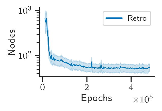
Figure 5: Validation curve for the retro branching agent on the $500\times 1000$ set covering test instances. Although most performance gains were made in the first $\approx 200\text{k}$ epochs, the agent did not stop improving, with the last recorded checkpoint improvement at $485\text{k}$ epochs.

Appendix B Neural Network

B.1 Architecture

We used the same gcn architecture as Gasse et al. 2019 to parameterise our dqn value function with some minor modifications which we found to be helpful. Firstly, we replaced the ReLU activations with Leaky ReLUs which we inverted in the final readout layer in order to predict the negative Q-values of our mdp. Secondly, we initialised our linear layer weights and biases with a normal distribution ($\mu=0,\sigma=0.01$) and all-zeros respectively, and our layer normalisation weights and biases with all-ones and all-zeros respectively. Thirdly, we removed a network forward pass in the bipartite graph convolution message passing operation which we found to be unhelpfully computationally expensive. For clarity, Figure 6 shows the high-level overview of the neural network architecture. For a full analysis of the benefit of using gcn for learning to branch, refer to Gasse et al. 2019.

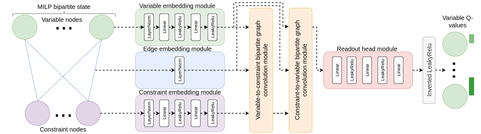
Figure 6: Neural network architecture used to parameterise the Q-value function for our ML agents, taking in a bipartite graph representation of the MILP and outputting the predicted Q-values for each variable in the MILP.

B.2 Inference & Solving Times

The key performance criterion to optimise for any branching method is the reduction of the overall bnb solving time. However, accurate and precise solving time and primal-dual integral over time comparisons are difficult because they are hardware-dependent. This is particularly problematic in research settings where CPU/GPU resources are often shared between multiple researchers and therefore hardware performance (and consequently solving time) significantly varies. Consequently, as in other works (Khalil et al. 2016; Gasse et al. 2019; Etheve et al. 2020), we presented and optimised for the number of bnb tree nodes as this is hardware-independent and, in the context of prior work, can be used to infer the solving time.

Specifically, we use the same gcn-based architecture of Gasse et al. 2019 for all ml branchers, thus all ml approaches have the same per-step inference cost. Therefore the relative difference in the number of tree nodes is exactly the relative wall-clock times on equal hardware. When the per-step inference process is different (as for our non-ml baselines, such as sb), the number of tree nodes is not an adequate proxy for solving time. However, Gasse et al. 2019 have already demonstrated that the gcn-based branching policies of il outperform the solving time of other branchers such as sb. As this ml speed-up has already been established, in this manuscript we focus on improving the per-step ml decision quality using rl rather than further optimising network architecture, or otherwise, for speed, which we leave to further work.

However, empirical solving times are of interest to the broader optimisation community. Therefore, Table 3 provides a summary of the solving times of the branching agents on the large $500\times 1000$ set covering instances under the assumption that they were ran on the same hardware as Gasse et al. 2019.

Method	Solving time (s)
SB	$33.5$
IL	$2.1$
Retro	$2.5$
FMSTS-DFS	$12.2$
FMSTS	$7.6$
Original	$35.8$

Table 3: Inferred mean solving times of the branching agents on the large $500\times 1000$ set covering instances under the assumption that they were ran on the same hardware as Gasse et al. 2019.

Appendix C Data Set Size Analysis

As described in Section 5, we used $100$ milp instances unseen during training to evaluate the performance of each branching agent. This is in line with prior works such as Khalil et al. 2016 who used $84$ instances and Gasse et al. 2019 who used $20$. To ensure that $100$ instances are a large enough data set to reliably compare branching agents, we also ran the agents on $1000$ large $500\times 1000$ set covering instances. The relative performance of each branching agent was approximately the same as when evaluated on $100$ instances, with Retro scoring $65.3$ nodes, FMSTS $250$ ($3.8\times$ worse than Retro), il $55.4$ ($17.8\%$ better than Retro), and sb $43.3$. In the interest of saving evaluation time and hardware demands and to make the development of and comparison to our work by future research projects more accessible, as well as for clarity in the per-instance Retro-IL comparison of Figure 3d, we report the results for $100$ evaluation instances in the main paper in the knowledge that the relative performances are unchanged as we scale the data set to a larger size.

Appendix D SCIP Parameters

For all non-dfs branching agents we used the same SCIP 2022 bnb parameters as Gasse et al. 2019, as summarised in Table 4.

SCIP Parameter	Value
separating/maxrounds	$0$
separating/maxroundsroot	$0$
limits/time	$3600$

Table 4: Summary of the SCIP 2022 hyperparameters used for all non-dfs branching agents (any parameters not specified were the default SCIP 2022 values).

Appendix E Observation Features

We found it useful to add $20$ features to the variable nodes in the bipartite graph in addition to the $19$ features used by Gasse et al. 2019. These additional features are given in Table 5; their purpose was to help the agent to learn to aggregate over the uncertainty in the future primal-dual bound evolution caused by the partially observable activity occurring in sub-trees external to its retrospectively constructed trajectory.

Variable Feature	Description
db_frac_change	Fractional dual bound change
pb_frac_change	Fractional primal bound change
max_db_frac_change	Maximum possible fractional dual change
max_pb_frac_change	Maximum possible fractional primal change
gap_frac	Fraction primal-dual gap
num_leaves_frac	# leaves divided by # nodes
num_feasible_leaves_frac	# feasible leaves divided by # nodes
num_infeasible_leaves_frac	# infeasible leaves divided by # nodes
num_lp_iterations_frac	# nodes divded by # LP iterations
num_siblings_frac	Focus node’s # siblings divided by # nodes
is_curr_node_best	If focus node is incumbent
is_curr_node_parent_best	If focus node’s parent is incumbent
curr_node_depth	Focus node depth
curr_node_db_rel_init_db	Initial dual divided by focus’ dual
curr_node_db_rel_global_db	Global dual divided by focus’ dual
is_best_sibling_none	If focus node has a sibling
is_best_sibling_best_node	If focus node’s sibling is incumbent
best_sibling_db_rel_init_db	Initial dual divided by sibling’s dual
best_sibling_db_rel_global_db	Global dual divided by sibling’s dual
best_sibling_db_rel_curr_node_db	Sibling’s dual divided by focus’ dual

Table 5: Descriptions of the $20$ variable features we included in our observation in addition to the $19$ features used by Gasse et al. 2019.

Appendix F FMSTS Implementation

Etheve et al. (2020) did not open-source any code, used the paid commercial CPLEX (2009) solver, and experimented with proprietary data sets. Furthermore, they omitted comparisons to any other ml baseline such as Gasse et al. (2019), further limiting their comparability. However, we have done a ‘best effort’ implementation of the relatively simple fmsts algorithm, whose core idea is to set the Q-function of a dqn agent as minimising the sub-tree size rooted at the current node and to use a dfs node selection heuristic. To replicate the dfs setting of Etheve et al. (2020) in SCIP (2022), we used the parameters shown in Table 6. We will release the full re-implementation to the community along with our own code.

SCIP Parameter	Value
separating/maxrounds	$0$
separating/maxroundsroot	$0$
limits/time	$3600$
nodeselection/dfs/stdpriority	$1\,073\,741\,823$
nodeselection/dfs/memsavepriority	$536\,870\,911$
nodeselection/restartdfs/stdpriority	$-536\,870\,912$
nodeselection/restartdfs/memsavepriority	$-536\,870\,912$
nodeselection/restartdfs/selectbestfreq	$0$
nodeselection/bfs/stdpriority	$-536\,870\,912$
nodeselection/bfs/memsavepriority	$-536\,870\,912$
nodeselection/breadthfirst/stdpriority	$-536\,870\,912$
nodeselection/breadthfirst/memsavepriority	$-536\,870\,912$
nodeselection/estimate/stdpriority	$-536\,870\,912$
nodeselection/estimate/memsavepriority	$-536\,870\,912$
nodeselection/hybridestim/stdpriority	$-536\,870\,912$
nodeselection/hybridestim/memsavepriority	$-536\,870\,912$
nodeselection/uct/stdpriority	$-536\,870\,912$
nodeselection/uct/memsavepriority	$-536\,870\,912$

Table 6: Summary of the SCIP 2022 hyperparameters used the dfs fmsts branching agent of Etheve et al. 2020 (any parameters not specified were the default SCIP 2022 values).

Appendix G Pseudocode

Retrospective Trajectory Construction

Algorithm 1 shows the proposed ‘retrospective trajectory construction’ method, whereby fathomed leaf nodes not yet added to a trajectory are selected as the brancher’s terminal states and paths to them are iteratively established using some construction method.

Algorithm 1 Retrospectively construct trajectories.

  Input: bnb tree $\mathcal{T}$ from solving MILP

  Output: Retrospectively constructed trajectories

  Initialise: nodes_added, subtree_episodes = [$\mathcal{T}_{\text{root}-1}$], []

  // Construct trajectories until all valid node(s) in $\mathcal{T}$ added

  while True do

     // Root trajectories at highest level unselected node(s)

     subtrees = []

     for node in nodes_added do

        for child_node in $\mathcal{T_{\text{node}}}\text{.children}$ do

           if child_node not in nodes_added then

              // Use depth-first-search to get sub-tree

              subtrees.append(dfs($\mathcal{T}$, root=child_node))

           end if

        end for

     end for

     // Construct trajectory episode(s) from sub-tree(s)

     if $\text{len(subtrees)}>0$ then

        for subtree in subtrees do

           subtree_episode = construct_path(subtree) (2)

           subtree_episode[$-1$].done = True

           subtree_episodes.append(subtree_episode)

           for node in subtree_episode do

              nodes_added.append(node)

           end for

        end for

     else

        // All valid nodes in $\mathcal{T}$ added to a trajectory

        break

     end if

  end while

Maximum Leaf lp Gain

Algorithm 2 shows the proposed ‘maximum leaf lp gain’ trajectory construction method, whereby the fathomed leaf node with the greatest change in the dual bound (‘lp gain’) is used as the terminal state of the trajectory.

Algorithm 2 Maximum leaf LP gain trajectory construction.

  Input: Sub-tree $\mathcal{S}$

  Output: Trajectory $\mathcal{S}_{E}$

  Initialise: gains = {}

  for leaf in $\mathcal{S}\text{.leaves}$ do

     if leaf closed by brancher then

        gains.leaf = $|\mathcal{S}_{\text{root}}\text{.dual\_bound}-\mathcal{S}_{\text{leaf}}\text{.dual\_bound}|$

     end if

  end for

  terminal_node = max(gains)

  $\mathcal{S}_{E}$ = shortest_path(source=$\mathcal{S}_{\text{root}}$, target=terminal_node)

Appendix H Cost of Strong Branching Labels

As well as performance being limited to that of the expert imitated, il methods have the additional drawback of requiring an expensive data labelling phase. Figure 7 shows how the explore-then-strong-branch labelling scheme of Gasse et al. 2019 scales with set covering instance size ($\text{rows}\times{\text{columns}}$) and how this becomes a hindrance for larger instances. Although an elaborate infrastructure can be developed to try to label large instances at scale (Nair et al. 2021), ideally the need for this should be avoided; a key motivator for using rl to branch.

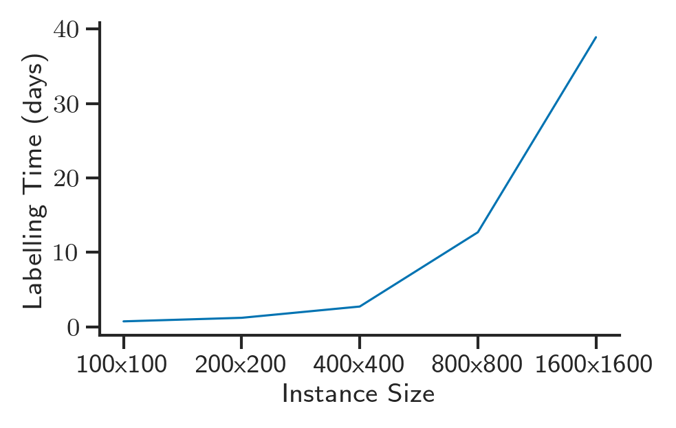
Figure 7: How the explore-then-strong-branch data labelling phase of the strong branching imitation agent scales with set covering instance size ($\text{rows}\times\text{columns}$) using an Intel Xeon ES-2660 CPU and assuming $120\,000$ samples are needed for each set.

References

- Achterberg (2007) Achterberg, T. 2007. Constraint Integer Programming. Doctoral thesis, Technische Universität Berlin, Fakultät II - Mathematik und Naturwissenschaften, Berlin.
- Achterberg, Koch, and Martin (2004) Achterberg, T.; Koch, T.; and Martin, A. 2004. Branching rules revisited. Technical Report 04-13, ZIB, Takustr. 7, 14195 Berlin.
- Achterberg and Wunderling (2013) Achterberg, T.; and Wunderling, R. 2013. Mixed Integer Programming: Analyzing 12 Years of Progress.
- Agostinelli et al. (2019) Agostinelli, F.; McAleer, S.; Shmakov, A.; and Baldi, P. 2019. Solving the Rubik’s cube with deep reinforcement learning and search. Nature Machine Intelligence, 1(8): 356–363.
- Alvarez, Louveaux, and Wehenkel (2017) Alvarez, A. M.; Louveaux, Q.; and Wehenkel, L. 2017. A Machine Learning-Based Approximation of Strong Branching. INFORMS J. Comput., 29: 185–195.
- Applegate et al. (2007) Applegate, D. L.; Bixby, R. E.; Chvatal, V.; and Cook, W. J. 2007. The Traveling Salesman Problem: A Computational Study. Princeton University Press.
- Applegate et al. (1995) Applegate, D. L.; Bixpy, R. E.; Chvatal, V.; and Cook, W. J. 1995. Finding cuts in the TSP (A preliminary report). Technical report, DIMACS.
- Balas, Ho, and Center (2018) Balas, E.; Ho, A.; and Center, C. M. U. R. 2018. Set covering algorithms using cutting planes, heuristics, and subgradient optimization : a computational study.
- Barahona (1982) Barahona, F. 1982. On the computational complexity of Ising spin glass models. Journal of Physics A: Mathematical and General, 15(10): 3241.
- Barnhart et al. (1998) Barnhart, C.; Johnson, E. L.; Nemhauser, G. L.; Savelsbergh, M. W. P.; and Vance, P. H. 1998. Branch-And-Price: Column Generation for Solving Huge Integer Programs. Oper. Res., 46(3): 316–329.
- Bengio, Lodi, and Prouvost (2021) Bengio, Y.; Lodi, A.; and Prouvost, A. 2021. Machine learning for combinatorial optimization: A methodological tour d’horizon. European Journal of Operational Research, 290(2): 405–421.
- Benichou et al. (1971) Benichou, M.; Gauthier, J. M.; Girodet, P.; Hentges, G.; Ribiere, G.; and Vincent, O. 1971. Experiments in mixed-integer linear programming. Mathematical Programming, 1(1): 76–94.
- Bergman et al. (2016) Bergman, D.; Cire, A. A.; Hoeve, W.-J. v.; and Hooker, J. 2016. Decision Diagrams for Optimization. Springer Publishing Company, Incorporated, 1st edition. ISBN 3319428470.
- Burda et al. (2018) Burda, Y.; Edwards, H.; Storkey, A.; and Klimov, O. 2018. Exploration by Random Network Distillation.
- Cappart et al. (2021) Cappart, Q.; Chételat, D.; Khalil, E.; Lodi, A.; Morris, C.; and Veličković, P. 2021. Combinatorial optimization and reasoning with graph neural networks.
- Conti et al. (2018) Conti, E.; Madhavan, V.; Such, F. P.; Lehman, J.; Stanley, K. O.; and Clune, J. 2018. Improving Exploration in Evolution Strategies for Deep Reinforcement Learning via a Population of Novelty-Seeking Agents. In Proceedings of the 32nd International Conference on Neural Information Processing Systems, NIPS’18, 5032–5043. Red Hook, NY, USA: Curran Associates Inc.
- CPLEX (2009) CPLEX, I. 2009. V12. 1: User’s Manual for CPLEX. International Business Machines Corporation, 46(53): 157.
- Ecoffet et al. (2021) Ecoffet, A.; Huizinga, J.; Lehman, J.; Stanley, K. O.; and Clune, J. 2021. First return, then explore. Nature, 590(7847): 580–586.
- Etheve et al. (2020) Etheve, M.; Alès, Z.; Bissuel, C.; Juan, O.; and Kedad-Sidhoum, S. 2020. Reinforcement Learning for Variable Selection in a Branch and Bound Algorithm. Lecture Notes in Computer Science, 176–185.
- Gasse et al. (2019) Gasse, M.; Chételat, D.; Ferroni, N.; Charlin, L.; and Lodi, A. 2019. Exact Combinatorial Optimization with Graph Convolutional Neural Networks. Red Hook, NY, USA: Curran Associates Inc.
- Geurts, Ernst, and Wehenkel (2006) Geurts, P.; Ernst, D.; and Wehenkel, L. 2006. Extremely randomized trees. Machine Learning, 63(1): 3–42.
- Harutyunyan et al. (2019) Harutyunyan, A.; Dabney, W.; Mesnard, T.; Heess, N.; Azar, M. G.; Piot, B.; van Hasselt, H.; Singh, S.; Wayne, G.; Precup, D.; and Munos, R. 2019. Hindsight Credit Assignment. Red Hook, NY, USA: Curran Associates Inc.
- He, Daumé, and Eisner (2014) He, H.; Daumé, H.; and Eisner, J. 2014. Learning to Search in Branch-and-Bound Algorithms. In Proceedings of the 27th International Conference on Neural Information Processing Systems - Volume 2, NIPS’14, 3293–3301. Cambridge, MA, USA: MIT Press.
- Hessel et al. (2017) Hessel, M.; Modayil, J.; van Hasselt, H.; Schaul, T.; Ostrovski, G.; Dabney, W.; Horgan, D.; Piot, B.; Azar, M.; and Silver, D. 2017. Rainbow: Combining Improvements in Deep Reinforcement Learning.
- Khalil et al. (2016) Khalil, E. B.; Bodic, P. L.; Song, L.; Nemhauser, G. L.; and Dilkina, B. N. 2016. Learning to Branch in Mixed Integer Programming. In AAAI.
- Korte and Vygen (2012) Korte, B. H.; and Vygen, J. 2012. Combinatorial Optimization: Theory and Algorithms. New York, NY: Springer-Verlag. ISBN 9783642244889 3642244882 3642244874 9783642244872.
- Land and Doig (1960) Land, A. H.; and Doig, A. G. 1960. An Automatic Method of Solving Discrete Programming Problems. Econometrica, 28(3): pp. 497–520.
- Leyton-Brown, Pearson, and Shoham (2000) Leyton-Brown, K.; Pearson, M.; and Shoham, Y. 2000. Towards a Universal Test Suite for Combinatorial Auction Algorithms. In Proceedings of the 2nd ACM Conference on Electronic Commerce, EC ’00, 66–76. New York, NY, USA: Association for Computing Machinery. ISBN 1581132727.
- Lillicrap et al. (2019) Lillicrap, T. P.; Hunt, J. J.; Pritzel, A.; Heess, N.; Erez, T.; Tassa, Y.; Silver, D.; and Wierstra, D. 2019. Continuous control with deep reinforcement learning.
- Lin (1992) Lin, L.-J. 1992. Self-Improving Reactive Agents Based on Reinforcement Learning, Planning and Teaching. Mach. Learn., 8(3–4): 293–321.
- Litvinchev and Ozuna Espinosa (2012) Litvinchev, I.; and Ozuna Espinosa, E. L. 2012. Solving the Two-Stage Capacitated Facility Location Problem by the Lagrangian Heuristic. In Hu, H.; Shi, X.; Stahlbock, R.; and Voß, S., eds., Computational Logistics, 92–103. Berlin, Heidelberg: Springer Berlin Heidelberg. ISBN 978-3-642-33587-7.
- Lodi and Zarpellon (2017) Lodi, A.; and Zarpellon, G. 2017. On learning and branching: a survey. TOP, 25(2): 207–236.
- Maher et al. (2016) Maher, S.; Miltenberger, M.; Pedroso, J. P.; Rehfeldt, D.; Schwarz, R.; and Serrano, F. 2016. PySCIPOpt: Mathematical Programming in Python with the SCIP Optimization Suite. In Mathematical Software – ICMS 2016, 301–307. Springer International Publishing.
- Mao et al. (2019) Mao, H.; Venkatakrishnan, S. B.; Schwarzkopf, M.; and Alizadeh, M. 2019. Variance Reduction for Reinforcement Learning in Input-Driven Environments. In 7th International Conference on Learning Representations, ICLR 2019, New Orleans, LA, USA, May 6-9, 2019. OpenReview.net.
- Mitchell (2009) Mitchell, J. E. 2009. Integer programming: branch and cut algorithmsInteger Programming: Branch and Cut Algorithms, 1643–1650. Boston, MA: Springer US. ISBN 978-0-387-74759-0.
- Mnih et al. (2013) Mnih, V.; Kavukcuoglu, K.; Silver, D.; Graves, A.; Antonoglou, I.; Wierstra, D.; and Riedmiller, M. 2013. Playing Atari with Deep Reinforcement Learning.
- Nair et al. (2021) Nair, V.; Bartunov, S.; Gimeno, F.; von Glehn, I.; Lichocki, P.; Lobov, I.; O’Donoghue, B.; Sonnerat, N.; Tjandraatmadja, C.; Wang, P.; Addanki, R.; Hapuarachchi, T.; Keck, T.; Keeling, J.; Kohli, P.; Ktena, I.; Li, Y.; Vinyals, O.; and Zwols, Y. 2021. Solving Mixed Integer Programs Using Neural Networks.
- Nelder and Mead (1965) Nelder, J. A.; and Mead, R. 1965. A simplex method for function minimization. Computer Journal, 7: 308–313.
- Perdomo-Ortiz et al. (2012) Perdomo-Ortiz, A.; Dickson, N.; Drew-Brook, M.; Rose, G.; and Aspuru-Guzik, A. 2012. Finding low-energy conformations of lattice protein models by quantum annealing. Scientific Reports, 2: 571.
- Prouvost et al. (2020) Prouvost, A.; Dumouchelle, J.; Scavuzzo, L.; Gasse, M.; Chételat, D.; and Lodi, A. 2020. Ecole: A Gym-like Library for Machine Learning in Combinatorial Optimization Solvers. In Learning Meets Combinatorial Algorithms at NeurIPS2020.
- Salimans and Chen (2018) Salimans, T.; and Chen, R. 2018. Learning Montezuma’s Revenge from a Single Demonstration.
- Schaul et al. (2016) Schaul, T.; Quan, J.; Antonoglou, I.; and Silver, D. 2016. Prioritized Experience Replay.
- SCIP (2022) SCIP. 2022. The SCIP Optimization Suite 7.0. Technical report, Optimization Online.
- Silver et al. (2016) Silver, D.; Huang, A.; Maddison, C. J.; Guez, A.; Sifre, L.; van den Driessche, G.; Schrittwieser, J.; Antonoglou, I.; Panneershelvam, V.; Lanctot, M.; Dieleman, S.; Grewe, D.; Nham, J.; Kalchbrenner, N.; Sutskever, I.; Lillicrap, T.; Leach, M.; Kavukcuoglu, K.; Graepel, T.; and Hassabis, D. 2016. Mastering the game of Go with deep neural networks and tree search. Nature, 529(7587): 484–489.
- Silver et al. (2017) Silver, D.; Schrittwieser, J.; Simonyan, K.; Antonoglou, I.; Huang, A.; Guez, A.; Hubert, T.; Baker, L.; Lai, M.; Bolton, A.; Chen, Y.; Lillicrap, T.; Hui, F.; Sifre, L.; van den Driessche, G.; Graepel, T.; and Hassabis, D. 2017. Mastering the game of Go without human knowledge. Nature, 550(7676): 354–359.
- Sutton (1988) Sutton, R. S. 1988. Learning to predict by the methods of temporal differences. Machine Learning, 3(1): 9–44.
- Sutton and Barto (2018) Sutton, R. S.; and Barto, A. G. 2018. Reinforcement Learning: An Introduction. The MIT Press, second edition.
- Tomazella and Nagano (2020) Tomazella, C. P.; and Nagano, M. S. 2020. A comprehensive review of Branch-and-Bound algorithms: Guidelines and directions for further research on the flowshop scheduling problem. Expert Systems with Applications, 158: 113556.
- Trott et al. (2019) Trott, A.; Zheng, S.; Xiong, C.; and Socher, R. 2019. Keeping Your Distance: Solving Sparse Reward Tasks Using Self-Balancing Shaped Rewards. In NeurIPS.
- van Hasselt, Guez, and Silver (2015) van Hasselt, H.; Guez, A.; and Silver, D. 2015. Deep Reinforcement Learning with Double Q-learning.
- Zarpellon et al. (2021) Zarpellon, G.; Jo, J.; Lodi, A.; and Bengio, Y. 2021. Parameterizing Branch-and-Bound Search Trees to Learn Branching Policies. arXiv:2002.05120.
- Zhang et al. (2021) Zhang, T.; Xu, H.; Wang, X.; Wu, Y.; Keutzer, K.; Gonzalez, J. E.; and Tian, Y. 2021. NovelD: A Simple yet Effective Exploration Criterion. In Beygelzimer, A.; Dauphin, Y.; Liang, P.; and Vaughan, J. W., eds., Advances in Neural Information Processing Systems.