Data-Driven Evolutionary Multi-Objective Optimization Based on Multiple-Gradient Descent for Disconnected Pareto Fronts 

Abstract: Data-driven evolutionary multi-objective optimization (EMO) has been recognized as an effective approach for multi-objective optimization problems with expensive objective functions. The current research is mainly developed for problems with a ‘regular’ triangle-like Pareto-optimal front (PF), whereas the performance can significantly deteriorate when the PF consists of disconnected segments. Furthermore, the offspring reproduction in the current data-driven EMO does not fully leverage the latent information of the surrogate model. Bearing these considerations in mind, this paper proposes a data-driven EMO algorithm based on multiple-gradient descent. By leveraging the regularity information provided by the up-to-date surrogate model, it is able to progressively probe a set of well distributed candidate solutions with a convergence guarantee. In addition, its infill criterion recommends a batch of promising candidate solutions to conduct expensive objective function evaluations. Experiments on $33$ benchmark test problem instances with disconnected PFs fully demonstrate the effectiveness of our proposed method against four selected peer algorithms.

Keywords: Data-driven optimization Multiple-gradient descent Evolutionary multi-objective optimization.

1 Introduction

Many real-world scientific and engineering applications involve multiple conflicting objectives, a.k.a. multi-objective optimization problems (MOPs). For example, tuning a water distribution system to optimize its financial and operational costs [1], minimizing the energy consumption while maximizing locomotion speed in a complex robotic system [2]. In multi-objective optimization, there does not exist a solution that optimizes all conflicting objectives simultaneously. Instead, we are looking for a set of representative, with a promising convergence and diversity, trade-off solutions that compromise one objective for another.

Due to the population-based characteristics, evolutionary algorithms (EAs) have been widely recognized as an effective approach for MO [3, 4]. However, one of the major criticisms of EAs is its daunting amount of function evaluations (FEs) required to obtain a set of reasonable solutions. This is unfortunately unacceptable in practice since FEs are either computationally or financially demanding, e.g., computational fluid dynamic simulations can take from minutes to hours to carry out a single FE [5]. To mitigate this issue, data-driven evolutionary optimization, guided by surrogate models of computationally expensive objective functions, have become as a powerful approach for solving expensive optimization problems [7]. For example, some researchers considered various ways to build a surrogate model of the expensive objective functions, either collectively [8, 9, 10, 11] or as a weighted aggregation [12, 13, 14, 15]. According to the ways of surrogate modeling, bespoke model management strategies are developed to select promising candidate solution(s) for conducting expensive FEs. In particular, this can either be driven by the surrogate model directly [14, 15, 9] or an acquisition function inferred from the model uncertainty [12, 13, 8, 10, 11]. There are two gaps in the current literature that hinder the further uptake of data-driven evolutionary multi-objective optimization (EMO) in practice.

• Most, if not all, existing studies are mainly designed and validated on prevalent test problems (e.g., DTLZ1 to DTLZ4 [16] and WFG4 to WFG9 [17]) characterized as ‘regular’ triangle-like Pareto-optimal fronts (PFs). Unfortunately, this is unrealistic in the real-world optimization scenarios [18]. On the contrary, it is not uncommon that the PFs of real-world applications are featured as disconnected, incomplete, degenerated, and/or badly-scaled (partially due to the complex and nonlinear relationship between objectives), it is surprising that the research on handling MOPs with irregular PFs is lukewarm in the context of data-driven EMO, except for [11].

• In addition, the evolutionary operators for offspring reproduction are directly derived from the EA (e.g., crossover and mutation [19], differential evolution [20], particle swarm optimization [21]) or conventional mathematical programming (e.g., simplex [22], Nelder–Mead [23], and trust-region methods [24]). By this means, the regularity information of the underlying MOP embedded in the surrogate model(s) is unfortunately yet exploited. Note that such information can be beneficial to navigate a more effective exploration of the search space.

Bearing these considerations in mind, this paper proposes a data-driven evolutionary multi-objective optimization based on multiple-gradient descent [25] for expensive MOPs with disconnected PFs. Its basic idea is to leverage the gradient information of the surrogate models to explore promising candidate solutions. It consists of the following two distinctive components.

• MGD-based evolutionary search: As the main crux of our proposed algorithm, it generates a set of candidate solutions guided by the multiple-gradient descent of the surrogate model of each computationally expensive objective function. In a nutshell, these candidate solutions are first randomly sampled in the decision space. Then, they are gradually guided to interpolate well distributed potential solutions along the manifold of the surrogate PS.

• Infill criterion: It recommends a batch of promising candidate solutions obtained by the MGD-based evolutionary search step to carry out expensive FEs for the model management.

Our experiments on $33$ benchmark test problem instances with disconnected PFs fully demonstrate the effectiveness and outstanding performance of our proposed D²EMO/MGD against four selected peer algorithms.

The rest of this paper is organized as follows. Section 2 gives some preliminary knowledge pertinent to this paper. The technical details of our proposed method is introduced in Section 3. The experimental setup is given in Section 4 and the results are presented and discussed in Section 5. Section 6 concludes this paper and sheds some lights on potential future directions.

2 Preliminaries

In this section, we give some basic definitions pertinent to this paper.

2.1 Basic Definitions in Multi-Objective Optimization

The MOP considered in this paper is defined as:

$$\begin{array}[]{l l}\mathrm{minimize}\quad\mathbf{F}(\mathbf{x})=(f_{1}(\mathbf{x}),\cdots,f_{m}(\mathbf{x}))^{T}\\ \mathrm{subject\ to}\;\;\mathbf{x}\in\Omega\end{array},$$ (1)

where $\mathbf{x}=(x_{1},\cdots,x_{n})^{T}$ is a decision vector and $\mathbf{F}(\mathbf{x})$ is an objective vector. $\Omega=[x_{i}^{L},x_{i}^{U}]^{n}_{i=1}\subseteq\mathbb{R}^{n}$ defines the search space. $\mathbf{F}:\Omega\rightarrow\mathbb{R}^{m}$ is the corresponding attainable set in the objective space $\mathbb{R}^{m}$.

Definition 1.

Given two solutions $\mathbf{x}^{1},\mathbf{x}^{2}\in\Omega$, $\mathbf{x}^{1}$ is said to Pareto dominate $\mathbf{x}^{2}$, denoted as $\mathbf{x}^{1}\preceq\mathbf{x}^{2}$, if and only if $f_{i}(\mathbf{x}^{1})\leq f_{i}(\mathbf{x}^{2})$ for all $i\in\{1,\cdots,m\}$ and $\mathbf{F}(\mathbf{x}^{1})\neq\mathbf{F}(\mathbf{x}^{2})$.

Definition 2.

A solution $\mathbf{x}^{\ast}\in\Omega$ is said to be Pareto-optimal if and only if $\nexists\mathbf{x}^{\prime}\in\Omega$ such that $\mathbf{x}^{\prime}\preceq\mathbf{x}^{\ast}$.

Definition 3.

The set of all Pareto-optimal solutions is called the Pareto-optimal set (PS), i.e., $\mathcal{PS}=\{\mathbf{x}^{\ast}|\nexists\mathbf{x}^{\prime}\in\Omega\text{ such that }\mathbf{x}^{\prime}\preceq\mathbf{x}^{\ast}\}$ and their corresponding objective vectors form the Pareto-optimal front (PF), i.e., $\mathcal{PF}=\{\mathbf{F}(\mathbf{x}^{\ast})|\mathbf{x}^{\ast}\in\mathcal{PS}\}$.

2.2 Gaussian Process Regression Model

In view of the continuously differentiable property, we consider the Gaussian process regression (GPR) [26] as the surrogate model of each expensive objective function. Given a set of training data $\mathcal{D}=\{(\mathbf{x}^{i},f(\mathbf{x}^{i})\}_{i=1}^{N}$, a GPR model aims to learn a latent function $g(\mathbf{x})$ by assuming $f(\mathbf{x}^{i})=g(\mathbf{x}^{i})+\epsilon$ where $\epsilon\sim\mathcal{N}(0,\sigma^{2}_{n})$ is an independently and identically distributed Gaussian noise. For each testing input vector $\mathbf{z}^{\ast}\in\Omega$, the mean and variance of the target $f(\mathbf{z}^{\ast})$ are predicted as:

$$\overline{g}(\mathbf{z}^{\ast}) =m(\mathbf{z}^{\ast})+{\mathbf{k}^{\ast}}^{T}(K+\sigma_{n}^{2}I)^{-1}(\mathbf{f}-\mathbf{m}(X)),$$ (2)

$$\mathbb{V}[g(\mathbf{z}^{\ast})] =k(\mathbf{z}^{\ast},\mathbf{z}^{\ast})-{\mathbf{k}^{\ast}}^{T}(K+\sigma_{n}^{2}I)^{-1}{\mathbf{k}^{\ast}},$$ (3)

where $X=(\mathbf{x}^{1},\cdots,\mathbf{x}^{N})^{T}$ and $\mathbf{f}=(f(\mathbf{x}^{1}),\cdots,f(\mathbf{x}^{N}))^{T}$. $\mathbf{m}(X)$ is the mean vector of $X$, $\mathbf{k}^{\ast}$ is the covariance vector between $X$ and $\mathbf{z}^{\ast}$, and $K$ is the covariance matrix of $X$. In this paper, we use the radial basis function as the covariance function to measure the similarity between a pair of two solutions $\mathbf{x}$ and $\mathbf{x}^{\prime}\in\Omega$:

$$k(\mathbf{x},\mathbf{x}^{\prime})=\gamma\exp(-\frac{\|\mathbf{x}-\mathbf{x}^{\prime}\|^{2}}{\ell}),$$ (4)

where $\|\cdot\|$ is the Euclidean norm and $\gamma$ and length scale $\ell$ are two hyperparameters. The predicted mean $\overline{g}(\mathbf{z}^{\ast})$ is directly used as the prediction of $f(\mathbf{z}^{\ast})$, and the predicted variance $\mathbb{V}[g(\mathbf{x}^{\ast})]$ quantifies the uncertainty. In practice, the hyperparameters associated with the mean and covariance functions are learned by maximizing the log marginal likelihood function as recommended in [26]. For the sake of simplicity, here we assume that the mean function is a constant $0$ and the inputs are noiseless.

3 Proposed Method

In this section, we plan to delineate the implementation of our proposed data-driven evolutionary multi-objective optimization based on multiple-gradient descent (dubbed D²EMO/MGD). As the flowchart shown in Fig. 1, D²EMO/MGD starts with an initialization step based on an experimental design method such as Latin hypercube sampling [27]. Note that these initial samples will be evaluated based on the computationally expensive objective functions. During the main loop, the surrogate modeling step builds a surrogate model by using the GPR for each expensive objective function based on the data collected so far. The other two steps will be delineated in the following paragraphs.

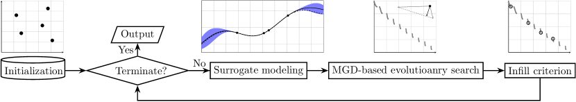
Figure 1: The flow chart of the proposed D²EMO/MGD.

3.1 MGD-based Evolutionary Search

This step aims to search for a set of promising candidate solutions $\mathcal{P}=\{\hat{\mathbf{x}}^{i}\}_{i=1}^{\tilde{N}}$, which are assumed to be an appropriate approximation to the PF, based on the surrogate model built in the surrogate modeling step. The working mechanism of this MGD-based evolutionary search step is given as follows.

1. Initialize a candidate solution set $\mathcal{P}=\{\hat{\mathbf{x}}^{i}\}_{i=1}^{\tilde{N}}$ based on Latin hypercube sampling upon $\Omega$.

2. For each solution $\hat{\mathbf{x}}^{i}\in\mathcal{P}$, do

   1. Calculate the gradient of the predicted mean of each objective function $\nabla\overline{g}_{j}(\hat{\mathbf{x}}^{i})$ where $j\in\{1,\cdots,m\}$.

   2. Find a nonnegative unit vector $\mathbf{w}^{\ast}=(w_{1}^{\ast},\cdots,w_{m}^{\ast})^{\top}$ that satisfies:

      $$\mathbf{w}^{\ast}=\operatorname*{argmin}_{\mathbf{w}}\bigg{\|}\sum_{j=1}^{m}w_{j}\nabla\overline{g}_{j}(\hat{\mathbf{x}}^{i})\bigg{\|},$$ (5)

      where $\mathbf{w}=(w_{1},\cdots,w_{m})^{\top}$, $\sum_{i=1}^{m}w_{i}=1$ and $w_{i}\geq 0$, $i\in\{1,\cdots,m\}$.

   3. Obtain a directional vector $\mathbf{u}^{\ast}$ as:

      $$\mathbf{u}^{\ast}=\begin{cases}\underset{1\leq j\leq m}{\operatorname*{argmax}}\big{\|}\nabla\overline{g}_{j}(\hat{\mathbf{x}}^{i})\big{\|},&\text{if }\sum_{j=1}^{m}w_{j}^{\ast}\nabla\overline{g}_{j}(\hat{\mathbf{x}}^{i})=0\\ \underset{1\leq j\leq m}{\operatorname*{argmin}}\big{\|}\nabla\overline{g}_{j}(\hat{\mathbf{x}}^{i})\big{\|},&\text{if }\exists i,j\in\{1,\cdots,m\},\langle\nabla\overline{g}_{j}(\hat{\mathbf{x}}^{i}),\nabla\overline{g}_{j}(\hat{\mathbf{x}}^{i})\rangle>\delta\\ \sum_{j=1}^{m}w_{j}^{\ast}\nabla\overline{g}_{j}(\hat{\mathbf{x}}^{i}),&\text{otherwise}\end{cases}$$ (6)

      where $\langle\ast,\ast\rangle$ measures the acute angle between two vectors, and $\delta=\min\Big{\{}\big{\|}\nabla\overline{g}_{k}(\hat{\mathbf{x}}^{i})\big{\|}\Big{\}}_{k=1}^{m}$.

   4. Amend the updated solution to $\mathcal{P}\leftarrow\mathcal{P}\bigcup\{\hat{\mathbf{x}}^{i}+\eta\mathbf{u}^{\ast}\}$

3. Remove the dominated solutions in $\mathcal{P}$ according to their predicted objective functions.

4. If the stopping criterion is met, then stop and output $\mathcal{P}$. Otherwise, go to Step 2.

Remark 1.

As discussed in [25], the multiple-gradient descent (MGD) is a natural extension of the single-objective gradient to finding a PF. In a nutshell, its basic idea is to iteratively update a solution $\mathbf{x}$ along a ‘specified’ direction so that all objective functions can thus be improved. Different from the linear weighted aggregation, the MGD works for non-convex PF. Therefore, we can expect a descent diversity in case the initial population is well distributed. Note that since the objective functions are assumed to be as a black box a priori, the MGD is not directly applicable in our context.

Remark 2.

In this paper, since the computationally expensive objective functions are modeled by GPR, which is continuously differentiable, we can derive the gradient of the predicted mean function w.r.t. a solution $\mathbf{x}$ as:

$$\frac{\partial\overline{g}(\mathbf{x})}{\partial\mathbf{x}}=\frac{\partial\mathbf{k}^{\ast}}{\partial\mathbf{x}}K^{-1}\mathbf{f},$$ (7)

where the first-order derivative of $\mathbf{k}^{\ast}$, i.e., the covariance vector between $\mathcal{P}$ and $\mathbf{x}$, is calculated as:

$$\frac{\partial\mathbf{k}^{\ast}}{\partial\mathbf{x}}=-\frac{\partial\|\mathbf{x}-\mathbf{x}^{\prime}\|}{\partial\mathbf{x}}\frac{\overline{g}(\mathbf{x})}{\ell}.$$ (8)

Remark 3.

The optimization problem in (5) is essentially equivalent to finding a minimum-norm point in the convex hull. When $m=2$, we have the closed form solution as:

$$w_{1}^{\ast}=\frac{\big{(}\nabla\overline{g}_{2}(\hat{\mathbf{x}}^{i})-\nabla\overline{g}_{1}(\hat{\mathbf{x}}^{i})\big{)}^{\top}\nabla\overline{g}_{2}(\hat{\mathbf{x}}^{i})}{\|\nabla\overline{g}_{2}(\hat{\mathbf{x}}^{i})-\nabla\overline{g}_{1}(\hat{\mathbf{x}}^{i})\big{\|}^{2}},\text{ }w_{2}^{\ast}=1-w_{1}^{\ast}.$$ (9)

Remark 4.

Fig. 2 gives an illustrative example for each of the three conditions given in equation (6) when $m=2$. More specifically, when the gradients of two objective functions are in opposite directions as shown in Fig. 2(a), $\mathbf{u}^{\ast}$ is chosen as the one with a larger Euclidean norm. If the gradients are too close to each other as shown in Fig. 2(b), $\mathbf{u}^{\ast}$ is chosen as the one with a smaller Euclidean norm. On the contrary, $\mathbf{u}^{\ast}$ is set as the weighted aggregation of two gradients where the weights are obtained from Step 2.2.

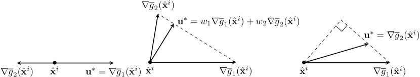
Figure 2: Illustrative examples of the calculation of $\mathbf{u}^{\ast}$ in equation (6).

Remark 5.

According to the Karush–Kuhn–Tucker (KKT) conditions [28], we have $\forall\mathbf{x}^{\ast}\in\mathcal{PS}$, $\exists\vec{\alpha}=(\alpha_{1},\cdots,\alpha_{m})^{T}$, where $\alpha_{i}\geq 0$, $i\in\{1,\cdots,m\}$ and $\sum_{i=1}^{m}\alpha_{i}=1$, such that $\sum_{i=1}^{m}\alpha_{i}\nabla f_{i}(\mathbf{x}^{\ast})=0$. In this case, we come up with Theorem 1 and Corollary 1, the proof of which can be found in the supplemental document of this paper.

Theorem 1.

Considering the $m$ objective functions defined in (1), $\forall\mathbf{x}\in\Omega$ but $\mathbf{x}\notin\mathcal{PS}$, $\exists\mathbf{w}^{\ast}$ that satisfies (5) and $\mathbf{u}^{\ast}=\sum_{j=1}^{m}w_{j}^{\ast}\nabla f_{j}(\mathbf{x})>0$, we can obtain a new solution $\mathbf{x}^{\prime}=\mathbf{x}+\eta\mathbf{u}^{\ast}$ such that $\mathbf{x}^{\prime}\preceq\mathbf{x}$.

Corollary 1.

Considering the $m$ objective functions defined in (1), $\forall\mathbf{x}\in\mathcal{PS}$, $\exists\mathbf{w}^{\ast}$ that satisfies (5) and $\mathbf{u}^{\ast}=\sum_{j=1}^{m}w_{j}^{\ast}\nabla f_{j}(\mathbf{x})=0$, we can obtain a new solution $\mathbf{x}^{\prime}=\mathbf{x}+\eta\mathbf{u}^{\ast}$ such that $\mathbf{x}^{\prime}$ is still on the PS.

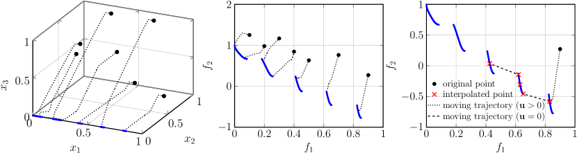
Figure 3: Illustrative examples of MGD w.r.t. different solutions moving towards different (a) PS segments and (b) PF segments, and (c) the working mechanismthe MGD-based evolutionary search step.

Remark 6.

According to Theorem 1, the MGD-based evolutionary search step can be understood as pushing a solution towards the PS first before implementing a random walk along the PS as an illustrative example shown in Fig. 3.

Remark 7.

In Step 2.4, $\eta\in(0,1]$ is a random scaling factor along the direction vector $\mathbf{u}^{\ast}$. The stopping criterion in Step 4 is the number of iterations (here it is set as $100$ in our experiments) of this MGD-based evolutionary search step.

3.2 Infill Criterion

This step aims to pick up $\xi\geq 1$ promising solutions from $\mathcal{P}$ and evaluate them by using the computationally expensive objective functions. These newly evaluated solutions are then used to update the training dataset for the next iteration. In a nutshell, there are two main difference w.r.t. many existing works on data-driven EA [7] and Bayesian optimization [29]. First, even though we the GPR as the surrogate model, our infill criterion does not rely on an uncertainty quantification measure, a.k.a. acquisition function. Second, instead of recommending one solution for the computationally expensive function evaluation in a sequential manner, the infill criterion step of D²EMO/MGD proposes to select a batch of samples at a time. Under a limited computational budget, we can expect to reduce the number of iterations of the main loop in Fig. 1 by $\xi$ times. In addition, since many physical experiments can be carried out in parallel given the availability of more than one infrastructure (e.g., the training and validating machine learning models are usually distributed into multiple cores or GPUs for hyper-parameter optimization in automated machine learning), such batched recommendation provides an actionable way for parallelization. Therefore, we can anticipate the practical importance to save the computational overhead. In this paper, we propose a simple infill criterion based on the individual Hypervolume [30] contribution (IHV). Specifically, the IHV of each candidate solution $\mathbf{x}\in\mathcal{P}$ is calculated as:

$$\mathtt{IHV}(\mathbf{x})=\mathtt{HV}(\mathcal{P})-\mathtt{HV}(\mathcal{P}\setminus\{\mathbf{x}\}),$$ (10)

where $\mathtt{HV}(\mathcal{P})$ evaluates the Hypervolume of $\mathcal{P}$. Then, the top $\xi$ solutions in $\mathcal{P}$ with the largest IHV are picked up for the expensive function evaluations.

4 Experimental Setup

This section introduces our experimental setup including the benchmark test problems, the peer algorithms along with their parameter settings, and the performance metrics and statistical tests.

4.1 Benchmark Test Problems

In our empirical study, we consider benchmark test problems with disconnect PF segments to constitute our benchmark suite, including ZDT3 [31], DTLZ7 [16] and WFG2 [17] along with their variants dubbed ZDT3$\star$, DTLZ7$\star$ and WFG2$\star$. Their mathematical definitions and characteristics can be found in the supplemental document. For each benchmark test problem, we set the number of objectives as $m=2$ and the number of variables as $n\in\{3,5,8\}$ respectively in our empirical study [32, 33, 34, 35, 36, 37, 38, 39, 40, 41, 42, 43, 44, 45, 46, 47, 48, 49, 50, 51, 52, 53, 54, 55, 56, 57, 58, 59, 60, 61, 62, 63, 64, 65].

4.2 Peer Algorithms and Parameter Settings

To validate the competitiveness of our proposed algorithm, we compare its performance with ParEGO [12], MOEA/D-EGO [13], K-RVEA [10], and HSMEA [11] widely used in the literature. We do not intend to delineate their working mechanisms here while interested readers are referred to their original papers for details. The parameter settings are listed as follows.

• Number of function evaluations (FEs): The initial sample size is set to $11\times n-1$ for all algorithms and the maximum number of FEs is capped as $250$.

• Reproduction operators: The parameters associated with the simulated binary crossover [66] and polynomial mutation [67] are set as $p_{c}=1.0$, $\eta_{c}=20$, $p_{m}=1/n$, $\eta_{m}=20$.

• Kriging models: As for the algorithms that use Kriging for surrogate modeling, the corresponding hyperparameters of the MATLAB Toolbox DACE [68] is set to be within the range $[10^{-5},10^{5}]$.

• Batch size $\xi$: It is set as $\xi=10$ for our proposed algorithms and $\xi=5$ is set in MOEA/D-EGO.

• Number of repeated runs: Each algorithm is independently run on each test problem for $31$ times with different random seeds.

4.3 Performance Metric and Statistical Tests

To have a quantitative evaluation of the performance of different algorithms, we use the widely used HV as the performance metric. To have a statistical interpretation of the significance of comparison results, we use the following three statistical measures in our empirical study.

• Wilcoxon signed-rank test [69]: This is a widely used non-parametric statistical test to conduct a pairwise comparison. In our experiments, we set the significance level as $p=0.05$.

• $A_{12}$ effect size [70]: This is an effect size measure that evaluates the probability of one algorithm is better than another. Specifically, given a pair of peer algorithms, $A_{12}=0.5$ means they are equivalent. $A_{12}>0.5$ denotes that one is better for more than 50% of the times. $0.56\leq A_{12}<0.64$ indicates a small effect size while $0.64\leq A_{12}<0.71$ and $A_{12}\geq 0.71$ mean a medium and a large effect size, respectively.

• Scott-knott test [71]: This is used to rank the performance of different peer algorithms over $31$ runs on each test problem. In a nutshell, it uses a statistical test and effect size to divide the performance of peer algorithms into several clusters. In particular, the performance of peer algorithms within the same cluster are statistically equivalent. The smaller the rank is, the better performance of the algorithm achieves.

5 Experimental Results

In this section, our empirical study aims to investigate: 1) the performance of our proposed D²EMO/MGD compared against the selected peer algorithms; and 2) the effectiveness of the MGD-based evolutionary search and the infill criterion steps of D²EMO/MGD.

5.1 Performance Comparisons with the Peer Algorithms

The statistical comparison results of the Wilcoxon signed-rank test of the HV values between our proposed D²EMO/MGD against the other peer algorithms are given in Table 1. From these results, it is clear to see that the HV values obtained by D²EMO/MGD are statistically significantly better than the other four peer algorithms in all comparisons. As the selected results of the population distribution obtained by different algorithms shown in Fig. 4, it is clear to see that the solutions obtained by D²EMO/MGD not only have a good convergence on the PF, but also have a descent distribution on all disconnected PF segments. In contrast, the other peer algorithms either struggle to converge to the PF or hardly approximate all segments. It is interesting to note that the performance of HSMEA and K-RVEA are acceptable on ZDT3 and DTLZ7$\ast$, which have a relatively small number of disconnected segments, whereas their performance deteriorate significantly when the number of disconnected segments becomes large.

In addition to the pairwise comparisons, we apply the Scott-knott test to classify their performance into different groups to facilitate a better ranking among these algorithms. Due to the large number of comparisons, it will be messy if we list all ranking results ($11\times 3=33$ in total). Instead, we pull all the Scott-knott test results together and show their distribution and variance as the bar charts with error bar in Fig. 5(a). From this results, we can see that our proposed D²EMO/MGD is the best algorithm in all comparisons, which confirm the observations from Table 1. In addition, to have a better understanding of the performance difference of D²EMO/MGD w.r.t. the other peer algorithms, we investigate the comparison results of $A_{12}$ effect size. From the bar charts shown in Fig. 5(b), it is clear to see that the better results achieved by D²EMO/MGD is consistently classified as statistically large.

Table 1: Comparison results of D²EMO/MGD with the peer algorithms

	$n$	D2EMO/MGD	HSMEA	K-RVEA	MOEA/D-EGO	ParEGO
ZDT3	3	1.3199(3.34E-3)	1.2914(5.99E-2)†	1.1814(1.77E-1)†	1.1831(9.85E-2)†	1.1549(4.84E-2)†
	5	1.3271(1.52E-3)	1.2888(7.93E-2)†	1.1842(7.44E-2)†	1.0566(1.58E-1)†	1.0364(1.57E-1)†
	8	1.3260(4.29E-3)	1.1901(1.53E-1)†	1.2394(1.16E-1)†	1.0050(1.14E-1)†	0.7974(1.09E-1)†
ZDT31	3	1.3813(2.64E-2)	1.3183(2.06E-1)†	1.0556(2.54E-1)†	1.0983(2.84E-1)†	1.0839(9.35E-2)†
	5	1.3706(2.74E-2)	1.3064(6.99E-2)†	1.1107(1.72E-1)†	1.0351(2.13E-1)†	1.0068(8.73E-2)†
	8	1.3655(7.06E-2)	1.1851(1.14E-1)†	1.1098(1.65E-1)†	0.9112(1.21E-1)†	0.8659(2.16E-1)†
ZDT32	3	1.2818(2.18E-2)	1.2309(9.73E-2)†	1.1852(7.96E-2)†	1.1265(4.74E-2)†	1.1170(1.52E-2)†
	5	1.2610(8.73E-2)	1.1801(9.62E-2)†	1.1359(6.86E-2)†	1.0960(6.78E-2)†	1.0801(1.07E-1)†
	8	1.2860(2.12E-2)	1.1604(9.41E-2)†	1.1550(8.02E-2)†	1.0355(1.04E-1)†	1.0175(1.15E-1)†
ZDT33	3	0.9089(6.31E-4)	0.8643(5.41E-2)†	0.8683(7.07E-2)†	0.8578(3.22E-2)†	0.8249(2.46E-2)†
	5	0.9075(1.04E-3)	0.8508(3.32E-2)†	0.8845(6.85E-2)†	0.8148(1.83E-2)†	0.7487(5.64E-2)†
	8	0.9036(7.43E-2)	0.8130(9.20E-2)†	0.8630(6.48E-2)†	0.7911(3.25E-2)†	0.7126(4.45E-2)†
WFG2	3	5.9298(3.99E-2)	5.7944(2.10E-1)†	5.7083(1.48E-1)†	4.9327(3.51E-1)†	4.6709(2.84E-1)†
	5	5.9799(3.14E-2)	5.8221(1.11E-1)†	5.4672(1.40E-1)†	4.6521(4.99E-1)†	4.5911(6.76E-1)†
	8	5.7457(6.63E-2)	5.1535(3.36E-1)†	5.1191(3.18E-1)†	4.0520(4.96E-1)†	3.8378(4.09E-1)†
WFG21	3	6.2155(4.87E-2)	5.5538(4.16E-1)†	5.5407(3.49E-1)†	4.9540(3.22E-1)†	4.8377(2.97E-1)†
	5	6.2630(2.37E-2)	5.0867(5.17E-1)†	5.5867(9.45E-2)†	4.7417(4.15E-1)†	4.6174(3.08E-1)†
	8	6.0309(5.79E-2)	4.5420(3.14E-1)†	5.2068(3.06E-1)†	4.0720(3.10E-1)†	3.9503(4.48E-1)†
WFG22	3	2.8400(6.29E-2)	2.8154(1.42E-1)†	2.5958(1.55E-1)†	2.0903(1.65E-1)†	2.0581(1.68E-1)†
	5	2.8638(6.03E-2)	2.6386(1.21E-1)†	2.3946(6.85E-2)†	1.8671(1.47E-1)†	1.9506(1.78E-1)†
	8	2.6378(1.14E-1)	2.0694(2.54E-1)†	1.8419(1.50E-1)†	1.3691(5.16E-1)†	1.3248(2.54E-1)†
WFG23	3	5.7030(3.45E-1)	5.6479(4.02E-1)†	5.4574(2.62E-1)†	4.9859(2.54E-1)†	5.0298(4.56E-1)†
	5	5.9445(9.55E-2)	5.3802(3.19E-1)†	5.4525(1.42E-1)†	4.9615(2.60E-1)†	4.7642(5.69E-1)†
	8	5.6221(9.38E-2)	4.7431(2.40E-1)†	4.8954(2.38E-1)†	4.2413(3.71E-1)†	4.0819(2.20E-1)†
DTLZ7	3	1.3234(7.52E-3)	1.3195(1.84E-2)†	1.2407(1.18E-2)†	1.2550(2.56E-2)†	1.2076(6.05E-2)†
	5	1.3330(1.29E-3)	1.3138(1.73E-2)†	1.2371(2.14E-2)†	1.2131(1.20E-1)†	1.1303(5.55E-2)†
	8	1.3297(2.99E-3)	1.3123(1.09E-2)†	1.2263(2.52E-2)†	1.1591(1.13E-1)†	1.0667(1.21E-1)†
DTLZ71	3	1.3996(2.64E-3)	1.3959(1.02E-2)†	1.3289(1.79E-2)†	1.2916(7.39E-1)†	1.2735(2.84E-2)†
	5	1.4040(2.96E-3)	1.3936(9.43E-3)†	1.3190(1.26E-2)†	1.2746(3.82E-1)†	1.0609(1.67E-1)†
	8	1.4034(4.42E-3)	1.3762(1.07E-1)†	1.3146(1.50E-2)†	1.0508(1.41E-1)†	0.9420(2.51E-1)†
DTLZ72	3	1.4013(9.67E-3)	1.4013(1.69E-2)†	1.3292(2.58E-2)†	1.3006(1.44E-1)†	1.2863(4.18E-2)†
	5	1.4075(2.62E-3)	1.3926(1.00E-2)†	1.3313(1.72E-2)†	1.1908(1.14E-1)†	1.2150(6.59E-2)†
	8	1.4052(2.34E-3)	1.3875(1.20E-1)†	1.3170(1.53E-2)†	1.0411(8.06E-2)†	0.9540(2.36E-1)†

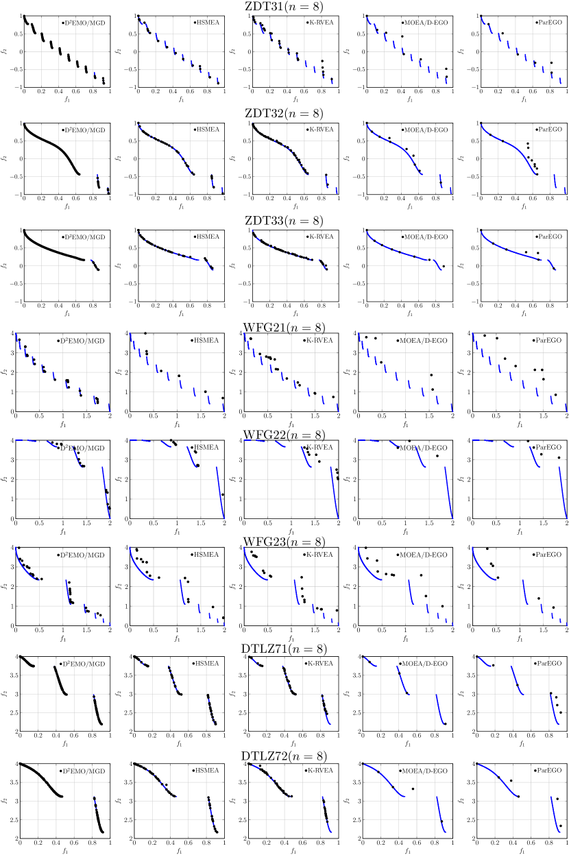
Figure 4: Non-dominated solutions obtained by different algorithms (with the medium HV values) on ZDT3$\ast$, WFG2$\ast$, and DTLZ7$\ast$ ($n=8$), respectively.

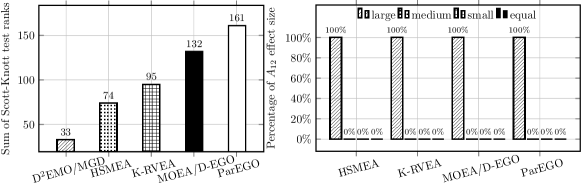
Figure 5: Statistical test results: (a) sum of the Scott-knott test results on all comparisons; (b) percentage of the equal, large, medium and small $A_{12}$ effect size, respectively, when comparing D²EMO/MGD against the other four peer algorithms.

5.2 Ablation Study

In this subsection, we empirically investigate the effectiveness of two key algorithmic components of D²EMO/MGD. More specifically, we first compare the performance of D²EMO/MGD w.r.t. the variant D²EMO/MGD-$v1$ without using the MGD-based evolutionary search step. Instead, it applies the widely used simulated binary crossover [66] as the alternative operator for offspring reproduction. From the selected results shown in Fig. 6, we can see that D²EMO/MGD-$v1$ can only find a very limited number of solutions on the PF with a poor diversity. Thereafter, we compare the performance of D²EMO/MGD w.r.t. the variant D²EMO/MGD-$v2$ without using the infill criterion introduced in Section 3.2. In particular, it uses a random selection to recommend the candidates for expensive function evaluations. From the selected results shown in Fig. 6, we can see that D²EMO/MGD-$v2$ can only find some of the disconnected PF segments.

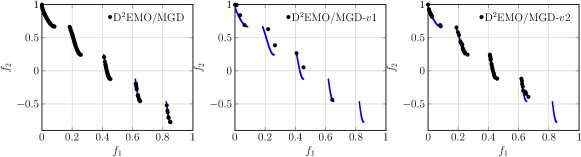
Figure 6: Non-dominated solutions (with the medium HV value) found by different variants of D²EMO/MGD on ZDT3 with $n=8$.

6 Conclusion

Most, if not all, existing data-driven EMO algorithms, directly apply evolutionary operators for offspring reproduction, while the regularity information embedded in the surrogate models has been unfortunately ignored. Bearing this consideration in mind, this paper, for the first time, investigates the use of MGD to leverage the latent information of the surrogate models to accelerate the convergence of the evolutionary population towards the PF. Due to the extra diversity provided by the exploration along the approximated PS manifold, our proposed D²EMO/MGD has shown strong performance on the selected benchmark test problems with disconnected PF segments. In addition, the ablation study also confirms the usefulness of the batched infill criterion guided by the IHV. Since this paper only considers problems with two objectives, its first potential extension is the scalability for problems with many objectives. In addition, it is well known that a biased mapping between the decision variables and the objective functions can raise significant challenges in EMO [72]. This will be aggravated when using the MGD, since the gradients along the approximated PS manifold can be largely biased towards a local niche. In addition, it is also interesting to investigate the performance of data-driven EMO algorithms for constrained multi-objective optimization problems [73, 74, 75, 76, 77].

References

- [1] J. Marques, M. C. Cunha, and D. A. Savic, “Multi-objective optimization of water distribution systems based on a real options approach,” Environ. Model. Softw., vol. 63, pp. 1–13, 2015.
- [2] R. Ariizumi, M. Tesch, H. Choset, and F. Matsuno, “Expensive multiobjective optimization for robotics with consideration of heteroscedastic noise,” in RSJ’14: Proc. of the 2014 IEEE/RSJ International Conference on Intelligent Robots and Systems. IEEE, 2014, pp. 2230–2235.
- [3] K. Deb, Multi-Objective Optimization Using Evolutionary Algorithms. New York, NY, USA: John Wiley & Sons, Inc., 2001.
- [4] G. Lai, M. Liao, and K. Li, “Empirical studies on the role of the decision maker in interactive evolutionary multi-objective optimization,” in CEC’21: Proc. of the 2021 IEEE Congress on Evolutionary Computation. IEEE, 2021, pp. 185–192.
- [5] Y. Jin and B. Sendhoff, “A systems approach to evolutionary multiobjective structural optimization and beyond,” IEEE Comp. Int. Mag., vol. 4, no. 3, pp. 62–76, 2009.
- [6] Y. Jin, “A comprehensive survey of fitness approximation in evolutionary computation,” Soft Comput., vol. 9, no. 1, pp. 3–12, 2005.
- [7] Y. Jin, H. Wang, T. Chugh, D. Guo, and K. Miettinen, “Data-driven evolutionary optimization: An overview and case studies,” IEEE Trans. Evol. Comput., vol. 23, no. 3, pp. 442–458, 2019.
- [8] I. Loshchilov, M. Schoenauer, and M. Sebag, “Dominance-based Pareto-surrogate for multi-objective optimization,” in SEAL’10: Proc. of the 8th International Conference Simulated Evolution and Learning, ser. Lecture Notes in Computer Science, vol. 6457. Springer, 2010, pp. 230–239.
- [9] T. Akhtar and C. A. Shoemaker, “Multi-objective optimization of computationally expensive multi-modal functions with RBF surrogates and multi-rule selection,” J. Glob. Optim., vol. 64, no. 1, pp. 17–32, 2016.
- [10] T. Chugh, Y. Jin, K. Miettinen, J. Hakanen, and K. Sindhya, “A surrogate-assisted reference vector guided evolutionary algorithm for computationally expensive many-objective optimization,” IEEE Trans. Evol. Comput., vol. 22, no. 1, pp. 129–142, 2018.
- [11] A. Habib, H. K. Singh, T. Chugh, T. Ray, and K. Miettinen, “A multiple surrogate assisted decomposition-based evolutionary algorithm for expensive multi/many-objective optimization,” IEEE Trans. Evol. Comput., vol. 23, no. 6, pp. 1000–1014, 2019.
- [12] J. D. Knowles, “ParEGO: a hybrid algorithm with on-line landscape approximation for expensive multiobjective optimization problems,” IEEE Trans. Evol. Comput., vol. 10, no. 1, pp. 50–66, 2006.
- [13] Q. Zhang, W. Liu, E. P. K. Tsang, and B. Virginas, “Expensive multiobjective optimization by MOEA/D with Gaussian process model,” IEEE Trans. Evol. Comput., vol. 14, no. 3, pp. 456–474, 2010.
- [14] G. Sun, G. Li, Z. Gong, G. He, and Q. Li, “Radial basis functional model for multi-objective sheet metal forming optimization,” Eng. Optim., vol. 43, no. 12, pp. 1351–1366, 2011.
- [15] S. Z. Martínez and C. A. C. Coello, “MOEA/D assisted by RBF networks for expensive multi-objective optimization problems,” in GECCO’13: Proc. of the 2013 Genetic and Evolutionary Computation Conference. ACM, 2013, pp. 1405–1412.
- [16] K. Deb, L. Thiele, M. Laumanns, and E. Zitzler, “Scalable test problems for evolutionary multiobjective optimization,” in Evolutionary Multiobjective Optimization, ser. Advanced Information and Knowledge Processing. Springer, 2005, pp. 105–145.
- [17] S. Huband, P. Hingston, L. Barone, and R. L. While, “A review of multiobjective test problems and a scalable test problem toolkit,” IEEE Trans. Evol. Comput., vol. 10, no. 5, pp. 477–506, 2006.
- [18] H. Ishibuchi, L. He, and K. Shang, “Regular Pareto front shape is not realistic,” in CEC’19: Proc. of the 2019 IEEE Congress on Evolutionary Computation. IEEE, 2019, pp. 2034–2041.
- [19] J. H. Holland, “Genetic algorithms and the optimal allocation of trials,” SIAM J. Comput., vol. 2, no. 2, pp. 88–105, 1973. [Online]. Available: https://doi.org/10.1137/0202009
- [20] R. Storn and K. V. Price, “Differential evolution - A simple and efficient heuristic for global optimization over continuous spaces,” J. Glob. Optim., vol. 11, no. 4, pp. 341–359, 1997. [Online]. Available: https://doi.org/10.1023/A:1008202821328
- [21] J. Kennedy and R. Eberhart, “Particle swarm optimization,” in Proceedings of International Conference on Neural Networks (ICNN’95), Perth, WA, Australia, November 27 - December 1, 1995. IEEE, 1995, pp. 1942–1948. [Online]. Available: https://doi.org/10.1109/ICNN.1995.488968
- [22] J. C. Dickson and F. P. Frederick, “A decision rule for improved efficiency in solving linear programming problems with the simplex algorithm,” Commun. ACM, vol. 3, no. 9, pp. 509–512, 1960. [Online]. Available: https://doi.org/10.1145/367390.367411
- [23] J. A. Nelder and R. Mead, “A simplex method for function minimization,” Comput. J., vol. 7, no. 4, pp. 308–313, 1965. [Online]. Available: https://doi.org/10.1093/comjnl/7.4.308
- [24] M. J. D. Powell, “On the global convergence of trust region algorithms for unconstrained minimization,” Math. Program., vol. 29, no. 3, pp. 297–303, 1984. [Online]. Available: https://doi.org/10.1007/BF02591998
- [25] J. Désidéri, “Multiple-gradient descent algorithm for Pareto-front identification,” in Modeling, Simulation and Optimization for Science and Technology, ser. Computational Methods in Applied Sciences, W. Fitzgibbon, Y. A. Kuznetsov, P. Neittaanmäki, and O. Pironneau, Eds. Springer, 2014, vol. 34, pp. 41–58.
- [26] C. E. Rasmussen and C. K. I. Williams, Gaussian processes for machine learning, ser. Adaptive computation and machine learning. MIT Press, 2006.
- [27] T. J. Santner, B. J. Williams, and W. I. Notz, The Design and Analysis of Computer Experiments, Second Edition. Springer-Verlag, 2018.
- [28] H. W. Kuhn and A. W. Tucker, “Nonlinear programming,” in Proc. of the 2nd Berkeley Symposium on Mathematical Statistics and Probability. Berkeley, CA, USA: University of California Press, 1951, pp. 481–492.
- [29] P. I. Frazier, “A tutorial on Bayesian optimization,” CoRR, vol. abs/1807.02811, 2018. [Online]. Available: http://arxiv.org/abs/1807.02811
- [30] E. Zitzler and L. Thiele, “Multiobjective evolutionary algorithms: a comparative case study and the strength Pareto approach,” IEEE Trans. Evol. Comput., vol. 3, no. 4, pp. 257–271, 1999.
- [31] E. Zitzler, K. Deb, and L. Thiele, “Comparison of multiobjective evolutionary algorithms: Empirical results,” Evol. Comput., vol. 8, no. 2, pp. 173–195, 2000.
- [32] K. Li, J. Zheng, C. Zhou, and H. Lv, “An improved differential evolution for multi-objective optimization,” in CSIE’09: Proc. of 2009 WRI World Congress on Computer Science and Information Engineering, 2009, pp. 825–830.
- [33] K. Li, J. Zheng, M. Li, C. Zhou, and H. Lv, “A novel algorithm for non-dominated hypervolume-based multiobjective optimization,” in SMC’09: Proc. of 2009 the IEEE International Conference on Systems, Man and Cybernetics, 2009, pp. 5220–5226.
- [34] J. Cao, H. Wang, S. Kwong, and K. Li, “Combining interpretable fuzzy rule-based classifiers via multi-objective hierarchical evolutionary algorithm,” in SMC’11: Proc. of the 2011 IEEE International Conference on Systems, Man and Cybernetics. IEEE, 2011, pp. 1771–1776.
- [35] K. Li, S. Kwong, R. Wang, J. Cao, and I. J. Rudas, “Multi-objective differential evolution with self-navigation,” in SMC’12: Proc. of the 2012 IEEE International Conference on Systems, Man, and Cybernetics, 2012, pp. 508–513.
- [36] K. Li, S. Kwong, J. Cao, M. Li, J. Zheng, and R. Shen, “Achieving balance between proximity and diversity in multi-objective evolutionary algorithm,” Inf. Sci., vol. 182, no. 1, pp. 220–242, 2012.
- [37] K. Li, S. Kwong, R. Wang, K. Tang, and K. Man, “Learning paradigm based on jumping genes: A general framework for enhancing exploration in evolutionary multiobjective optimization,” Inf. Sci., vol. 226, pp. 1–22, 2013.
- [38] K. Li and S. Kwong, “A general framework for evolutionary multiobjective optimization via manifold learning,” Neurocomputing, vol. 146, pp. 65–74, 2014.
- [39] J. Cao, S. Kwong, R. Wang, and K. Li, “AN indicator-based selection multi-objective evolutionary algorithm with preference for multi-class ensemble,” in ICMLC’14: Proc. of the 2014 International Conference on Machine Learning and Cybernetics, 2014, pp. 147–152.
- [40] K. Li, Á. Fialho, S. Kwong, and Q. Zhang, “Adaptive operator selection with bandits for a multiobjective evolutionary algorithm based on decomposition,” IEEE Trans. Evolutionary Computation, vol. 18, no. 1, pp. 114–130, 2014.
- [41] K. Li, Q. Zhang, S. Kwong, M. Li, and R. Wang, “Stable matching-based selection in evolutionary multiobjective optimization,” IEEE Trans. Evol. Comput., vol. 18, no. 6, pp. 909–923, 2014.
- [42] M. Wu, S. Kwong, Q. Zhang, K. Li, R. Wang, and B. Liu, “Two-level stable matching-based selection in MOEA/D,” in SMC’15: Proc. of the 2015 IEEE International Conference on Systems, Man, and Cybernetics, 2015, pp. 1720–1725.
- [43] K. Li, S. Kwong, Q. Zhang, and K. Deb, “Interrelationship-based selection for decomposition multiobjective optimization,” IEEE Trans. Cybernetics, vol. 45, no. 10, pp. 2076–2088, 2015.
- [44] K. Li, S. Kwong, and K. Deb, “A dual-population paradigm for evolutionary multiobjective optimization,” Inf. Sci., vol. 309, pp. 50–72, 2015.
- [45] K. Li, K. Deb, and Q. Zhang, “Evolutionary multiobjective optimization with hybrid selection principles,” in CEC’15: Proc. of the 2015 IEEE Congress on Evolutionary Computation, 2015, pp. 900–907.
- [46] K. Li, K. Deb, Q. Zhang, and Q. Zhang, “Efficient nondomination level update method for steady-state evolutionary multiobjective optimization,” IEEE Trans. Cybernetics, vol. 47, no. 9, pp. 2838–2849, 2017.
- [47] M. Wu, S. Kwong, Y. Jia, K. Li, and Q. Zhang, “Adaptive weights generation for decomposition-based multi-objective optimization using gaussian process regression,” in GECCO’17: Proc. of the 2017 Genetic and Evolutionary Computation Conference. ACM, 2017, pp. 641–648.
- [48] M. Wu, K. Li, S. Kwong, Y. Zhou, and Q. Zhang, “Matching-based selection with incomplete lists for decomposition multiobjective optimization,” IEEE Trans. Evolutionary Computation, vol. 21, no. 4, pp. 554–568, 2017.
- [49] K. Li, K. Deb, and X. Yao, “R-metric: Evaluating the performance of preference-based evolutionary multiobjective optimization using reference points,” IEEE Trans. Evolutionary Computation, vol. 22, no. 6, pp. 821–835, 2018.
- [50] R. Chen, K. Li, and X. Yao, “Dynamic multiobjectives optimization with a changing number of objectives,” IEEE Trans. Evol. Comput., vol. 22, no. 1, pp. 157–171, 2018.
- [51] T. Chen, K. Li, R. Bahsoon, and X. Yao, “FEMOSAA: feature-guided and knee-driven multi-objective optimization for self-adaptive software,” ACM Trans. Softw. Eng. Methodol., vol. 27, no. 2, pp. 5:1–5:50, 2018.
- [52] M. Wu, K. Li, S. Kwong, Q. Zhang, and J. Zhang, “Learning to decompose: A paradigm for decomposition-based multiobjective optimization,” IEEE Trans. Evolutionary Computation, vol. 23, no. 3, pp. 376–390, 2019.
- [53] K. Li, R. Chen, D. A. Savic, and X. Yao, “Interactive decomposition multiobjective optimization via progressively learned value functions,” IEEE Trans. Fuzzy Systems, vol. 27, no. 5, pp. 849–860, 2019.
- [54] K. Li, “Progressive preference learning: Proof-of-principle results in MOEA/D,” in EMO’19: Proc. of the 10th International Conference Evolutionary Multi-Criterion Optimization, 2019, pp. 631–643.
- [55] H. Gao, H. Nie, and K. Li, “Visualisation of pareto front approximation: A short survey and empirical comparisons,” in CEC’19: Proc. of the 2019 IEEE Congress on Evolutionary Computation, 2019, pp. 1750–1757.
- [56] K. Li, Z. Xiang, and K. C. Tan, “Which surrogate works for empirical performance modelling? A case study with differential evolution,” in CEC’19: Proc. of the 2019 IEEE Congress on Evolutionary Computation, 2019, pp. 1988–1995.
- [57] J. Zou, C. Ji, S. Yang, Y. Zhang, J. Zheng, and K. Li, “A knee-point-based evolutionary algorithm using weighted subpopulation for many-objective optimization,” Swarm and Evolutionary Computation, vol. 47, pp. 33–43, 2019.
- [58] M. Liu, K. Li, and T. Chen, “DeepSQLi: deep semantic learning for testing SQL injection,” in ISSTA’20: Proc. of the 29th ACM SIGSOFT International Symposium on Software Testing and Analysis. ACM, 2020, pp. 286–297.
- [59] K. Li, Z. Xiang, T. Chen, and K. C. Tan, “BiLO-CPDP: Bi-level programming for automated model discovery in cross-project defect prediction,” in ASE’20: Proc. of the 35th IEEE/ACM International Conference on Automated Software Engineering. IEEE, 2020, pp. 573–584.
- [60] K. Li, M. Liao, K. Deb, G. Min, and X. Yao, “Does preference always help? A holistic study on preference-based evolutionary multiobjective optimization using reference points,” IEEE Trans. Evol. Comput., vol. 24, no. 6, pp. 1078–1096, 2020.
- [61] M. Wu, K. Li, S. Kwong, and Q. Zhang, “Evolutionary many-objective optimization based on adversarial decomposition,” IEEE Trans. Cybern., vol. 50, no. 2, pp. 753–764, 2020.
- [62] K. Li, Z. Xiang, T. Chen, S. Wang, and K. C. Tan, “Understanding the automated parameter optimization on transfer learning for cross-project defect prediction: an empirical study,” in ICSE’20: Proc. of the 42nd International Conference on Software Engineering. ACM, 2020, pp. 566–577.
- [63] R. Wang, S. Ye, K. Li, and S. Kwong, “Bayesian network based label correlation analysis for multi-label classifier chain,” Inf. Sci., vol. 554, pp. 256–275, 2021.
- [64] L. Li, Q. Lin, K. Li, and Z. Ming, “Vertical distance-based clonal selection mechanism for the multiobjective immune algorithm,” Swarm Evol. Comput., vol. 63, p. 100886, 2021.
- [65] L. Chen, H. Liu, K. C. Tan, and K. Li, “Transfer learning-based parallel evolutionary algorithm framework for bilevel optimization,” IEEE Trans. Evol. Comput., vol. 26, no. 1, pp. 115–129, 2022.
- [66] K. Deb and R. B. Agrawal, “Simulated binary crossover for continuous search space,” Complex Systems, vol. 9, 1994.
- [67] K. Deb and M. Goyal, “A combined genetic adaptive search (GeneAS) for engineering design,” Computer Science and Informatics, vol. 26, pp. 30–45, 1996.
- [68] H. B. Nielsen, S. N. Lophaven, and J. Søndergaard, “DACE — A MATLAB Kriging toolbox,” Richard Petersens Plads, Building 321, DK-2800 Kgs. Lyngby, 2002.
- [69] F. Wilcoxon, “Individual comparisons by ranking methods,” 1945.
- [70] A. Vargha and H. D. Delaney, “A critique and improvement of the cl common language effect size statistics of mcgraw and wong,” J. Educ. Behav. Stat., vol. 25, no. 2, pp. 101–132, 2000.
- [71] N. Mittas and L. Angelis, “Ranking and clustering software cost estimation models through a multiple comparisons algorithm,” IEEE Trans. Software Eng., vol. 39, no. 4, pp. 537–551, 2013.
- [72] K. Deb, “Multi-objective genetic algorithms: Problem difficulties and construction of test problems,” Evol. Comput., vol. 7, no. 3, pp. 205–230, 1999.
- [73] K. Li, R. Chen, G. Fu, and X. Yao, “Two-archive evolutionary algorithm for constrained multiobjective optimization,” IEEE Trans. Evolutionary Computation, vol. 23, no. 2, pp. 303–315, 2019.
- [74] J. Billingsley, K. Li, W. Miao, G. Min, and N. Georgalas, “A formal model for multi-objective optimisation of network function virtualisation placement,” in EMO’19: Proc. of the 10th International Conference Evolutionary Multi-Criterion Optimization, 2019, pp. 529–540.
- [75] ——, “Parallel algorithms for the multiobjective virtual network function placement problem,” in EMO’21: Proc. of the 11th International Conference on Evolutionary Multi-Criterion Optimization, ser. Lecture Notes in Computer Science, vol. 12654. Springer, 2021, pp. 708–720.
- [76] X. Shan and K. Li, “An improved two-archive evolutionary algorithm for constrained multi-objective optimization,” in EMO’21: Proc. of the 11th International Conference on Evolutionary Multi-Criterion Optimization, ser. Lecture Notes in Computer Science, vol. 12654. Springer, 2021, pp. 235–247.
- [77] L. Yang, X. Hu, and K. Li, “A vector angles-based many-objective particle swarm optimization algorithm using archive,” Appl. Soft Comput., vol. 106, p. 107299, 2021.