Bias in the Representative Volume Element method:
periodize the ensemble instead of its realizations

Abstract.

We study the Representative Volume Element (RVE) method, which is a method to approximately infer the effective behavior $a_{\rm hom}$ of a stationary random medium. The latter is described by a coefficient field $a(x)$ generated from a given ensemble $\langle\cdot\rangle$ and the corresponding linear elliptic operator $-\nabla\cdot a\nabla$. In line with the theory of homogenization, the method proceeds by computing $d=3$ correctors ($d$ denoting the space dimension). To be numerically tractable, this computation has to be done on a finite domain: the so-called “representative” volume element, i. e. a large box with, say, periodic boundary conditions. The main message of this article is: Periodize the ensemble instead of its realizations.

By this we mean that it is better to sample from a suitably periodized ensemble than to periodically extend the restriction of a realization $a(x)$ from the whole-space ensemble $\langle\cdot\rangle$. We make this point by investigating the bias (or systematic error), i. e. the difference between $a_{\rm hom}$ and the expected value of the RVE method, in terms of its scaling w. r. t. the lateral size $L$ of the box. In case of periodizing $a(x)$, we heuristically argue that this error is generically $O(L^{-1})$. In case of a suitable periodization of $\langle\cdot\rangle$, we rigorously show that it is $O(L^{-d})$. In fact, we give a characterization of the leading-order error term for both strategies, and argue that even in the isotropic case it is generically non-degenerate.

We carry out the rigorous analysis in the convenient setting of ensembles $\langle\cdot\rangle$ of Gaussian type, which allow for a straightforward periodization, passing via the (integrable) covariance function. This setting has also the advantage of making the Price theorem and the Malliavin calculus available for optimal stochastic estimates of correctors. We actually need control of second-order correctors to capture the leading-order error term. This is due to inversion symmetry when applying the two-scale expansion to the Green function. As a bonus, we present a stream-lined strategy to estimate the error in a higher-order two-scale expansion of the Green function.

1. Introduction and statement of rigorous result

1.1. Uniformly elliptic coefficient fields

The basic objects of this paper are $\lambda$-uniformly elliptic tensor fields $a=a(x)$ (that are not necessarily symmetric) in $d$-dimensional space, by which we mean that for all points $x$

(1) $$\xi\cdot a(x)\xi\geq\lambda|\xi|^{2}\quad\mbox{and}\quad\xi\cdot a(x)\xi\geq|a(x)\xi|^{2}\quad\mbox{for all}\;\xi\in\mathbb{R}^{d}.$$

Such a tensor field $a$ gives rise to the heterogeneous elliptic operator $-\nabla\cdot a\nabla$ acting on functions $u$.

Homogenization means assimilating the effective, i. e. large-scale, behavior of a heterogeneous medium to a homogeneous one, as described by the constant tensor $a_{\rm hom}$. By this one means that the difference of the solution operators $(-\nabla\cdot a\nabla)^{-1}$ $-(-\nabla\cdot a_{\rm hom}\nabla)^{-1}$ converges to zero when applied to functions $f$ varying only on scales $L\uparrow\infty$. Homogenization is known to take place in a number of situations, see [59] for a general notion, e. g. when the coefficient field $a$ is periodic or when it is sampled from a stationary and ergodic ensemble $\langle\cdot\rangle$. While we are interested in the latter, it is convenient to introduce the Representative Volume Element (RVE) method in the context of the former.

1.2. The RVE method

Unless $d=1$, there is no explicit formula that allows to compute in practice $a_{\rm hom}$ for a general ensemble $\langle\cdot\rangle$. Early work treated specific ensembles that admit asymptotic explicit formulas in limiting regimes, like spherical inclusions covering a low volume fraction in [50, p. 365]. Explicit upper and lower bounds on $a_{\rm hom}$ in terms of features of the ensemble $\langle\cdot\rangle$ play a major role in the engineering literature, see for instance [51, 60]. On the contrary, the RVE method is a computational method to obtain convergent approximations to $a_{\rm hom}$ for a general the ensemble $\langle\cdot\rangle$. As the name “volume element” indicates, it is based on samples $a$ of $\langle\cdot\rangle$ in a (computational) domain, typically a cube of side-length $L$. It consists in inverting $-\nabla\cdot a\nabla$ for $d$ (representative) boundary conditions. The question of the appropriate size $L$ of the RVE evolved from a philosophical one in [36] (large enough to be statistically typical and so that boundary effects are dominated by bulk effects) towards a more practical one in [17] (just large enough so that the statistical properties relevant for the physical quantity $a_{\rm hom}$ are captured). The convergence of the method has been extensively investigated by numerical experiments in the engineering literature, see some references below. In this paper, we rigorously analyze some aspects of the convergence for a certain class of ensembles $\langle\cdot\rangle$.

We now introduce the RVE method. Suppose (momentarily) that the coefficient field $a$ is $L$-periodic, meaning that $a(x+Lk)=a(x)$ for all $x$ and $k\in\mathbb{Z}^{d}$. Given a Cartesian coordinate direction $i=1,\cdots,d$ and denoting by $e_{i}$ the unit vector in the $i$-th direction, we define (up to additive constants) $\phi_{i}^{(1)}$ as the $L$-periodic solution of

(2) $$-\nabla\cdot a(\nabla\phi_{i}^{(1)}+e_{i})=0.$$

The function $\phi_{i}^{(1)}$ is called first-order corrector, because it additively corrects the affine coordinate function $x_{i}$ in such a way that the resulting function $x\mapsto x_{i}+\phi_{i}^{(1)}(x)$ is $a$-harmonic, by which we understand that it vanishes under application of $-\nabla\cdot a\nabla$.

Let us momentarily adopt the language of a conducting medium: On the microscopic level, multiplication with the tensor field $a$ converts the electric field into the electric flux. On the macroscopic level, it is $a_{\rm hom}$ that relates the averaged field to the averaged flux. In view of (2), $\nabla\phi_{i}^{(1)}+e_{i}$ can be considered as an electric field in the absence of charges, arising from the electric potential $-(\phi_{i}^{(1)}+x_{i})$. In view of the periodicity of $\phi_{i}^{(1)}$, the large-scale average of $\nabla\phi_{i}^{(1)}+e_{i}$ is just $e_{i}$. Now $a(\nabla\phi_{i}^{(1)}+e_{i})$ is the corresponding flux. It is periodic, so its large-scale average is given by its average on the periodic cell

(3) $$\bar{a}e_{i}:=\fint_{[0,L)^{d}}a(\nabla\phi_{i}^{(1)}+e_{i}).$$

Observe that the notation $\bar{a}$ without reference to the period $L$ is legitimate since (3) is equivalent to $\bar{a}e_{i}$ $=\lim_{R\uparrow\infty}\fint_{[0,R)^{d}}a(\nabla\phi_{i}^{(1)}+e_{i})$. A well-known feature of homogenization is that $\bar{a}$ inherits the bounds (1) from $a$, as can be derived with help of the dual problem (20). In the periodic case, (3) in fact coincides with the homogenized coefficient $a_{\rm hom}$.

On the contrary, in the random case which we introduce now, (3) provides only a fluctuating approximation to the deterministic $a_{\rm hom}$. Homogenization is known to take place when $a$ is sampled from a stationary and ergodic ensemble $\langle\cdot\rangle$, see [38, 54]. By the latter we mean a probability measure on the space of tensor fields $a$ satisfying (1); we use the symbol $\langle\cdot\rangle$ to address both the ensemble and to denote its expectation operator. Stationarity is the crucial structural assumption and means that the shifted random field $x\mapsto a(z+x)$ has the same (joint) distribution as $a$ for any shift vector $z\in\mathbb{R}^{d}$. Ergodicity is a qualitative assumption that encodes the decorrelation of the values of $a$ over large distances.

1.3. Two strategies of periodizing

In order to apply the RVE method in form of (3), considered as an approximation for $a_{\rm hom}$, one needs to produce samples $a$ of $L$-periodic coefficient fields connected to the given ensemble $\langle\cdot\rangle$. The goal of this paper is to compare two strategies to procure such $L$-periodic samples. The first strategy relies on “periodizing the realizations” in its most naive form – we shall actually consider a seemingly less naive form of it, see Section 4 – and goes as follows: Taking a coefficient field $a$ in $\mathbb{R}^{d}$, we restrict it to the box $[0,L)^{d}$ and then periodically extend it. This defines a map $a\mapsto a_{L}$. We then take $\overline{a_{L}}$, cf. (3), as an approximation for $a_{\rm hom}$. One unfavorable aspect of this strategy is obvious: The push-forward of $\langle\cdot\rangle$ under this map $a\mapsto a_{L}$ is no longer stationary – an imagined glance at a typical realization would reveal $d$ families of parallel artificial hypersurfaces.

Related variants of this strategy consist in still restricting $a$ to $[0,L)^{d}$ but then imposing Dirichlet or Neumann boundary conditions instead of periodic boundary conditions (Neumann conditions will actually be analyzed in Section 4). Both boundary conditions for the random (vector) field $\nabla\phi^{(1)}=\nabla\phi^{(1)}(a,x)$ destroy its shift-covariance: It is no longer true that for any shift-vector $z\in\mathbb{R}^{d}$ we have $\nabla\phi^{(1)}(a,z+x)$ $=\nabla\phi^{(1)}(a(z+\cdot),x)$.

The second strategy relies on “periodizing the ensemble” and is more subtle: Given an ensemble $\langle\cdot\rangle$, one constructs a “related” stationary ensemble $\langle\cdot\rangle_{L}$ of $L$-periodic fields, samples $a$ from $\langle\cdot\rangle_{L}$ and takes $\bar{a}$ as an approximation. The quality of this second method was numerically explored in [35] for random non-overlapping inclusions, and (next to the first strategy) in [40] for random Voronoi tesselations; in both cases the periodization is obvious. Requirements on the periodization of ensembles were formulated in [56, Section 4], a general construction idea was given in [28, Remark 5]. In this paper, we advocate thinking of the map $\langle\cdot\rangle\leadsto\langle\cdot\rangle_{L}$ as conditioning on periodicity, and will construct it for a specific but relevant class of $\langle\cdot\rangle$ given in Assumption 1.

The second strategy obviously capitalizes on the knowledge of the ensemble $\langle\cdot\rangle$ and not just of a single realization (a “snapshot”), in the sense of “known unknowns” as opposed to “unknown unknowns”. This is in contrast with the numerical analysis on inferring $a_{\rm hom}$ in [52], or on constructing effective boundary conditions in [48, 49] from a snapshot.

1.4. Fluctuations and bias

In this paper, we are interested in comparing these two strategies in terms of their bias (also called systematic error): How much do the two expected values $\langle\overline{a_{L}}\rangle$ and $\langle\bar{a}\rangle_{L}$ deviate from $a_{\rm hom}$, which by qualitative theory is their common limit for $L\uparrow\infty$ (see [15] for $\langle\overline{a_{L}}\rangle$ and Corollary 1 $iii)$ for $\langle\overline{a}\rangle_{L}$). We shall heuristically argue that

(4) $$\langle\overline{a_{L}}\rangle-a_{\rm hom}=O(L^{-1}),$$

see Section 4, while proving

(5) $$\langle\bar{a}\rangle_{L}-a_{\rm hom}=O(L^{-d}),$$

see Theorems 1 and 2. Here $L$ should be thought of as the (non-dimensional) ratio between the actual period $L$ and a suitably defined correlation length of $\langle\cdot\rangle$ set to unity. The quantification of the convergence in $L$ is clearly of practical interest: After a discretization that resolves the correlation length, the number of unknowns of the linear algebra problem (2) scales with $L^{d}$ for $L\gg 1$. Numerical experiments confirm the $O(L^{-d})$ scaling [42, Figure 5] and the substantially worse behavior (4) for the other strategy [57]. In this regard, result (4) is not unexpected either from a theoretical or a numerical perspective, cf. [24, (3.4)], [15] and [23], respectively. Nevertheless, to the best of our knowledge, we provide here the first formal argument in favor of such a behavior.

We note that fluctuations (which are at the origin of the random part of the error), as for instance measured in terms of the square root of the variance, are in many situations proven to be of the order (see, e.g., [28, Theorem 2])

(6) $$\langle|\bar{a}-\langle\bar{a}\rangle_{L}|^{2}\rangle_{L}^{\frac{1}{2}}=O(L^{-\frac{d}{2}}),$$

see e.g. [42, Figure 6] for a numerical validation, and the same is expected to hold for the other strategy ([61, Fig.3] and [24, (3.3)])

$$\langle|\overline{a_{L}}-\langle\overline{a_{L}}\rangle|^{2}\rangle^{\frac{1}{2}}=O(L^{-\frac{d}{2}}).$$

Hence the variance scales like the inverse of the volume $L^{d}$ of the periodic cell $[0,L)^{d}$, as if we were averaging over $[0,L)^{d}$ some field of unit range of dependence instead of the long-range correlated $a(\nabla\phi_{i}+e_{i})$. In view of this identical fluctuation scaling for both strategies, the different bias scaling is significant in the most relevant dimension $d=3$, which we mostly focus in this paper: For the first strategy, the bias dominates, so that taking the empirical mean of $\overline{a_{L}}$ over many realizations $a$ does not substantially reduce the total error. It does so in the second scenario, which suggests to use variance reduction methods, like analyzed in [46, 25].

Theoretical results on the random error in RVE, at least for the second strategy like in (6), are by now abundant, starting from [30, Theorem 2.1] for a discrete medium with i. i. d. coefficient, over [27, Theorem 1] for a class of continuum media based on the Poisson point process, to the leading-order identification of the variance in in [19, Theorem 2]. The last result arises from the characterization of leading-order variances in stochastic homogenization in general, starting from [53, Theorem 2.1] for correctors, and is in the spirit of the general approach laid out in [34]. These estimates of variances and fluctuations in homogenization rely on a functional calculus (Malliavin derivatives, Spectral Gap inequalities). There is an alternative approach based on a finite range assumption (and its relaxation via mixing conditions) that was shown to yield optimal results in [3, 31], and culminated in the monograph [4]. In this paper, we make use of the first approach.

Theoretical results on the systematic error in RVE, again for the second strategy as in (5), seem to have been restricted to the case of a discrete medium with i. i. d. coefficients, see [28, Proposition 3], where the construction of $\langle\cdot\rangle_{L}$ is obvious. The argument for [28, Proposition 3] is based on a (necessarily non-stationary) coupling of $\langle\cdot\rangle$ and $\langle\cdot\rangle_{L}$, and introduces a massive term into the corrector equation in order to screen the resulting boundary layer, which leads to a logarithmically worse estimate than (5). Our analysis avoids this coupling and suggests that such a logarithmic correction is artificial. (Incidentally, the phenomenon that the bias decays to an order that is twice the order of the fluctuation decay occurs also in the analysis of the homogenization error $(-\nabla\cdot a\nabla)^{-1}f-(-\nabla\cdot a_{\rm hom}\nabla)^{-1}f$ itself: While the variance can be characterized to order $O(L^{-d})$, where $L\gg 1$ now is the ratio between the scale of $f$ and the correlation length, see [20, Theorem 1], the expectation seems to be characterized to order $O(L^{-2d})$, see [14, 44, 18].)

The first strategy is appealing since it only requires a snapshot, which could come from an actual material image, whereas the second one requires knowledge of the underlying ensemble, which has to be estimated or imposed as a model. Several methods to overcome the effect of boundary layers on the first strategy have been proposed: Motivated by the treatment of periodic coefficient fields of unknown period and the ensuing resonance error, oversampling [37] and filtering [11] strategies were proposed. Until recently, in case of random media however, because of the slow decay of the boundary layer, they were not expected to perform better than $O(L^{-1})$, see [24, (3.4)]. This motivated [26] to screen the boundary effects by a massive term to the corrector equation (2), cf. (53). However, results in preparation [8] suggest that, in the case of an isotropic ensemble, oversampling strategies may give rise to an improved rate $O(L^{-d/2})$ for the systematic error. Screening strategies based on semi-group [1, 52] or wave-equation [2] versions of the corrector equation have also been analyzed. Screening by a massive term, in conjunction with extrapolation in the massive parameter, has been proven to reduce the systematic error to $O(L^{-d})$ [28, Thm. 2]. Based on screening and extrapolation, [52, Prop. 1.1 & Th. 1.2] formulated a numerical algorithm that extracts $a_{\rm hom}$ from a snapshot $a$ up to the optimal total error $O(L^{-\frac{d}{2}})$ with only $O(L^{d})$ operations.

1.5. Assumptions and formulation of rigorous result

We now introduce a class of ensembles $\langle\cdot\rangle$ of $\lambda$-uniform coefficient fields $a$ that can be easily periodized. Loosely speaking, the natural way to periodize a general stationary ensemble $\langle\cdot\rangle$ of coefficient fields $a$ on $\mathbb{R}^{d}$ is to condition on $a$ being $L$-periodic. Clearly, this conditioning is highly singular, and we thus shall restrict ourselves to stationary and centered Gaussian ensembles $\langle\cdot\rangle$. Since a realization $g$ of such a Gaussian ensemble is obviously not ($\lambda$-uniformly) elliptic, we will work with a (nonlinear) map $A$ and consider the pointwise transformation $a(x)=A(g(x))$. More precisely, we will identify $\langle\cdot\rangle$ with its push-forward under

(7) $$g\mapsto a:=\big{(}x\mapsto A(g(x))\big{)}.$$

Centered Gaussian ensembles on some (infinite-dimensional) Banach space $X$ are characterized through their covariance, which is a semi-definite bounded bilinear form on $X^{*}$, defining a Hilbert space $H\subset X$. When $H$ is a Hilbert space of Hölder continuous functions on $\mathbb{R}^{d}$, this operator is best represented by its kernel $c(x,y)=\langle g(x)g(y)\rangle$. Stationarity of $\langle\cdot\rangle$ then amounts to $c=c(x-y)$; the positive-semidefinite character of the bilinear form translates into non-negativity of the Fourier transform ${\mathcal{F}}c(q)\geq 0$ for all wave vectors $q\in\mathbb{R}^{d}$. We now argue that periodization by conditioning can be characterized as follows: $\langle\cdot\rangle_{L}$ is the stationary centered Gaussian measure with $L$-periodic covariance $c_{L}$ with Fourier coefficients given by restricting the Fourier transform ${\mathcal{F}}c(q)$ to the dual lattice $q\in\frac{2\pi}{L}\mathbb{Z}^{d}$, defining the $k$-th Fourier mode of $c_{L}$ as :

(8) $$\frac{1}{\sqrt{L^{d}}}\int_{[0,L)^{d}}dx\,e^{-i\frac{2\pi k}{L}\cdot x}c_{L}(x):=\frac{1}{\sqrt{L^{d}}}{\mathcal{F}}c(\frac{2\pi k}{L})\;\;\mbox{for all}\;k\in\mathbb{Z}^{d}.$$

Since loosely speaking, the contributions to $\langle\cdot\rangle$ from every wave vector $q\in\mathbb{R}^{d}$ are independent, this restriction indeed corresponds to conditioning. This definition also highlights that information is lost when passing from $\langle\cdot\rangle$ to $\langle\cdot\rangle_{L}$. In terms of real space, the passage from $c$ to $c_{L}$ amounts to periodization of the covariance function:

(9) $$c_{L}(x)=\sum_{k\in\mathbb{Z}^{d}}c(x+Lk).$$

As for the whole space ensemble, we identify $\langle\cdot\rangle_{L}$ with its push-forward under (7).

We now collect the technical assumptions on $\langle\cdot\rangle$, that is, on the covariance function $c$ and the map $A$. Loosely speaking, we need that $A$ is regular and that $c$ is regular with integrable decay, both up to second derivatives .

Assumption 1.

Let $\langle\cdot\rangle$ be a stationary and centered Gaussian ensemble of scalar fields $g$ on $\mathbb{R}^{d}$, as determined by the covariance function $c(x):=\langle g(x)g(0)\rangle$. We assume that there exists an $\alpha>0$ such that

(10) $$\sup_{x\in\mathbb{R}^{d}}(1+|x|^{2})^{\frac{d+2}{2}+\alpha}|\nabla^{2}c(x)|<\infty.$$

We identify $\langle\cdot\rangle$ with its push-forward under the map (7), where $A\colon\mathbb{R}\rightarrow\mathbb{R}^{d\times d}$ is such that the coefficient field $a$ is $\lambda$-uniformly elliptic, see (1). We assume that

(11) $$\sup_{g\in\mathbb{R}}|A^{\prime}(g)|+|A^{\prime\prime}(g)|<\infty.$$

On the one hand, (10) implies by integration $\sup_{x\in\mathbb{R}^{d}}(1+|x|^{2})^{\frac{d}{2}+\alpha}|c(x)|<\infty$ and thus because of $\alpha>0$

(12) $$\sup_{q\in\mathbb{R}^{d}}{\mathcal{F}}c(q)\lesssim\int dx|c(x)|<\infty.$$

Via (8), (12) yields that the Cameron-Martin norm of $\langle\cdot\rangle_{L}$ dominates the $L^{2}([0,L)^{d})$-norm. This implies that $\langle\cdot\rangle_{L}$ endowed with the Hilbert structure of $L^{2}([0,L)^{d})$ has a uniform spectral gap in $L$, see [12, Poincaré inequality (5.5.2)]. By (11), this transmits to the ensemble of $a$’s, see (7), and will be used for the stochastic estimates.

On the other hand, (10) implies $\sup_{x}|\nabla^{2}c(x)|<\infty$ and thus $\sup_{x,y}|y-x|^{-2}\langle(g(y)$ $-g(x))^{2}\rangle$ $=\sup_{z}|z|^{-2}(c(0)$ $-c(z))$ $<\infty$. Since $g$ is Gaussian, this extends to arbitrary moments: $\sup_{x,y}|y-x|^{-1}$ $\langle|g(y)-g(x)|^{p}\rangle^{\frac{1}{p}}<\infty$. Estimating the Hölder semi-norm $[g]_{\alpha,B_{1}}^{p}$ by the Besov norm $\int_{B_{1}}dz|z|^{-d-p\alpha}\int_{B_{1}}dx|g(x+z)$ $-g(x)|^{p}$, one derives $\sup_{x}\langle[g]_{\alpha,B_{1}(x)}^{p}\rangle<\infty$ for any $\alpha<1$ and $p<\infty$. By (11), this transmits to the coefficient field $a$:

(13) $$\sup_{x}\langle\|a\|_{C^{0,\alpha}(B_{1}(x))}^{p}\rangle<\infty\quad\mbox{for all}\;\alpha<1,\;p<\infty,$$

which will allow us to appeal to Schauder theory for local regularity. Since because of (10) we also have $\sup_{L\geq 1}|\nabla^{2}c_{L}(x)|<\infty$, (13) extends to $\langle\cdot\rangle_{L}$ :

(14) $$\sup_{L\geq 1}\sup_{x}\langle\|a\|^{p}_{C^{0,\alpha}(B_{1}(x))}\rangle_{L}<\infty\quad\text{for any $\alpha<1$, $p<\infty$.}$$

Equipped with the definition of the periodized ensembles $\langle\cdot\rangle_{L}$, we can state our main result.

Theorem 1.

Let $d>2$ and $A$ be symmetric. Under the Assumption 1 on $\langle\cdot\rangle$, for all $L$, and with $\langle\cdot\rangle_{L}$ defined with (8) we have for the expectation $\langle\bar{a}\rangle_{L}$ of $\bar{a}$ defined in (3)

(15) $$\limsup_{L\uparrow\infty}L^{d}|\langle\bar{a}\rangle_{L}-a_{\rm hom}|<\infty.$$

Let us motivate the scaling (15). For fixed $i=1,\cdots,d$ we consider the flux

(16) $$q:=a(\nabla\phi^{(1)}_{i}+e_{i}),$$

which is a random (vector) field, meaning that $q=q(g,x)$. We note that by uniqueness for (2), $q$ is stationary, or rather “shift-covariant”, meaning that for every shift vector $z\in\mathbb{R}^{d}$, we have $q(g,z+x)=q(g(z+\cdot),x)$ for all points $x$ and (periodic) fields $g$. Hence by stationarity of $\langle\cdot\rangle_{L}$, we may write $\langle\bar{a}\rangle_{L}$ $=\langle q(0)\rangle_{L}$. Clearly, $q(0)$, as arising from the solution of the PDE (2), depends via $a=A(g)$ on the value of $g$ in any point $y$, no matter how distant from $0$.

Let us assume for a moment that $q$ were more local, meaning that $q(0)$ depends on $g$ only through its restriction $g_{|B_{R}}$ for some radius $R<\infty$. Let us also assume for simplicity that $\langle\cdot\rangle$ has unit range, which amounts to assume that $c$ is supported in $B_{1}$, a sharpening of (10). We then claim that

$$\langle q(0)\rangle_{L}\quad\mbox{is independent of}\;L\geq 2R+2.$$

Indeed, by the locality assumption and (centered) Gaussianity, the distribution of the value $q(0)=q(g,0)$ is determined by ${c_{L}}_{|B_{2R}}$. In view of (9) and by the finite range assumption, ${c_{L}}_{|B_{2R}}=c_{|B_{2R}}$ for $L\geq 1+2R+1$.

As mentioned, our flux $q(g,0)$ does depend on $g(y)$ even for $R=|y|\gg 1$. This dependence is described by the mixed derivative $\nabla\nabla G(a,0,y)$ of the Green function $G(a,x,y)$ for $-\nabla\cdot a\nabla$, see Subsection 2.2. Stochastic estimates show that, at least on an annealed level, the decay of this variable-coefficient Green’s function is no worse than of its constant-coefficient counterpart so that $R^{d}|\nabla\nabla G(a,0,y)|\lesssim 1$. Loosely speaking, it is this exponent $d$ that shows up in (15).

In the following Section 2, we will refine Theorem 1 by characterizing the leading-order error term in Theorem 2.

2. Theorem 1: refinement and main ideas

The two ingredients for Theorem 1 are a suitable representation formula for $\langle\bar{a}\rangle_{L}$, see Subsection 2.1, and its asymptotics through stochastic homogenization, here on the level of the mixed derivatives of the Green function, see Subsection 2.2. We need the second-order version of stochastic homogenization because of an inversion symmetry. We refine Theorem 1 in Subsection 2.3 by identifying the leading-order error term, see Theorem 2. In Subsection 2.4 we will argue that the leading-order error typically does not vanish, by exploring the regime of small ellipticity contrast. In Subsection 2.5 we discuss the structure of the leading-order error term in the case of an isotropic ensemble.

2.1. Representation formula

We start with an informal, but detailed, derivation of the representation formula, see (26), which might be the most conceptual piece of our work.

Let us fix two vectors $\xi$ and $\xi^{*}$ and focus on the component $\xi^{*}\cdot\bar{a}\xi$; we denote by $\phi^{(1)}$ the solution of (2) with $e_{i}$ replaced by $\xi$. By shift-covariance of $\nabla\phi^{(1)}$ and stationarity of $\langle\cdot\rangle_{L}$, we have

(17) $$\langle\xi^{*}\cdot\bar{a}\xi\rangle_{L}=\langle F\rangle_{L}\quad\mbox{where}\quad F:=(\xi^{*}\cdot a(\nabla\phi^{(1)}+\xi))(0).$$

Instead of directly estimating $\langle\xi^{*}\cdot\bar{a}\xi\rangle_{L}-\xi^{*}\cdot a_{\rm hom}\xi$, we will estimate its derivative w. r. t. $L$, that is $\frac{d}{dL}\langle\xi^{*}\cdot\bar{a}\xi\rangle_{L}$. The reason is that by general Gaussian calculus (in form of the Price formula) applied to the ensemble $\langle\cdot\rangle_{L}$ of (periodic) fields $g$ that depends on a parameter $L$, we have for any $F=F(g)$

(18) $$\frac{d}{dL}\langle F\rangle_{L}=\frac{1}{2}\int_{\mathbb{R}^{d}}dx\int_{\mathbb{R}^{d}}dy\Big{\langle}\frac{\partial^{2}F}{\partial g(-x)\partial g(-y)}\Big{\rangle}_{L}\frac{\partial c_{L}}{\partial L}(x-y),$$

where the two minus signs in the denominator are for later convenience. Here $\frac{\partial^{2}F}{\partial g(x)\partial g(y)}$ denotes the kernel representing the second Fréchet derivative of $F$, seen as a bilinear form on the space of functions on $\mathbb{R}^{d}$. As a derivative w. r. t. the noise $g$, it can be seen as a Malliavin derivative. We refer the reader to [16] for a rigorous proof of (18).

We define $F$ by (17). By the change of variables $z\rightsquigarrow x-y$, which capitalizes on the translation invariance of the covariance, and (more directly) by the stationarity of $\langle\cdot\rangle_{L}$ in conjunction with the stationarity of $\nabla\phi$ that leads to $\langle\frac{\partial^{2}F}{\partial g(-x)\partial g(z-x)}\rangle_{L}$ $=\langle\xi^{*}\cdot\frac{\partial^{2}a(\nabla\phi^{(1)}+\xi)(x)}{\partial g(0)\partial g(z)}\rangle_{L}$, we obtain

(19) $$\frac{d}{dL}\langle\xi^{*}\cdot\bar{a}\xi\rangle_{L}=\frac{1}{2}\int_{\mathbb{R}^{d}}dz\Big{\langle}\int_{\mathbb{R}^{d}}\xi^{*}\cdot\frac{\partial^{2}a(\nabla\phi^{(1)}+\xi)}{\partial g(0)\partial g(z)}\Big{\rangle}_{L}\frac{\partial c_{L}}{\partial L}(z).$$

With help of the corrector for the (pointwise) dual coefficient field $a^{*}$ in direction $\xi^{*}$, i. e. the periodic solution ${\phi^{*}}^{(1)}$ of

(20) $$\nabla\cdot a^{*}(\nabla{\phi^{*}}^{(1)}+\xi^{*})=0,$$

the inner integral can be rewritten more symmetrically as

$$\int_{\mathbb{R}^{d}}\xi^{*}\cdot\frac{\partial^{2}a(\nabla\phi^{(1)}+\xi)}{\partial g(0)\partial g(z)} =\int_{\mathbb{R}^{d}}(\nabla{\phi^{*}}^{(1)}+\xi^{*})\cdot\frac{\partial^{2}a(\nabla\phi^{(1)}+\xi)}{\partial g(0)\partial g(z)}$$

$$=\int_{\mathbb{R}^{d}}(\nabla{\phi^{*}}^{(1)}+\xi^{*})\cdot[\frac{\partial^{2}}{\partial g(0)\partial g(z)},a](\nabla\phi^{(1)}+\xi);$$

indeed, the first identity (formally) follows from applying $\frac{\partial^{2}}{\partial g(0)\partial g(z)}$ to (2) and then testing with ${\phi^{*}}^{(1)}$, whereas the second identify follows from testing (20) with $\frac{\partial^{2}\phi^{(1)}}{\partial g(0)\partial g(z)}$. Resolving the commutator $[\frac{\partial^{2}}{\partial g(0)\partial g(z)},a]$ by Leibniz’ rule we obtain

(21) $$\int_{\mathbb{R}^{d}}\xi^{*}\cdot\frac{\partial^{2}a(\nabla\phi^{(1)}+\xi)}{\partial g(0)\partial g(z)}= \int_{\mathbb{R}^{d}}(\nabla{\phi^{*}}^{(1)}+\xi^{*})\cdot\frac{\partial^{2}a}{\partial g(0)\partial g(z)}(\nabla\phi^{(1)}+\xi)$$

$$+\int_{\mathbb{R}^{d}}(\nabla{\phi^{*}}^{(1)}+\xi^{*})\cdot\frac{\partial a}{\partial g(0)}\nabla\frac{\partial\phi^{(1)}}{\partial g(z)}+\mbox{term with $z$, $0$ exchanged}.$$

Denoting $a^{\prime}:=A^{\prime}(g)$ and $a^{\prime\prime}:=A^{\prime\prime}(g)$, we remark that by (7) we have $\frac{\partial a(x)}{\partial g(z)}$ $=a^{\prime}(z)\delta(x-z)$. Applying operator $\frac{\partial}{\partial g(z)}$ on (2), we thus obtain the representation

(22) $$\frac{\partial\nabla\phi^{(1)}(x)}{\partial g(z)}=-\nabla\nabla G(x,z)a^{\prime}(z)(\nabla\phi+e)(z)$$

in terms of the mixed derivatives of the non-periodic Green function $G=G(a,x,y)$ associated with the operator $-\nabla\cdot a\nabla$. Hence the above turns into

$$\int_{\mathbb{R}^{d}}\xi^{*}\cdot\frac{\partial^{2}a(\nabla\phi^{(1)}+\xi)}{\partial g(0)\partial g(z)}= \delta(z)\big{(}(\nabla{\phi^{*}}^{(1)}+\xi^{*})\cdot a^{\prime\prime}(\nabla\phi^{(1)}+\xi)\big{)}(0)$$

$$-\big{(}a^{\prime}(\nabla{\phi^{*}}^{(1)}+\xi^{*})\big{)}(0)\cdot\nabla\nabla G(0,z)\big{(}a^{\prime}(\nabla\phi^{(1)}+\xi)\big{)}(z)$$

$$-\big{(}a^{\prime}(\nabla{\phi^{*}}^{(1)}+\xi^{*})\big{)}(z)\cdot\nabla\nabla G(z,0)\big{(}a^{\prime}(\nabla\phi^{(1)}+\xi)\big{)}(0).$$

Applying $\langle\cdot\rangle_{L}$ we obtain by stationarity

(23) $$\big{\langle}\int_{\mathbb{R}^{d}}\xi^{*}\cdot\frac{\partial^{2}a(\nabla\phi^{(1)}+\xi)}{\partial g(0)\partial g(z)}\big{\rangle}_{L}= \delta(z)\big{\langle}(\nabla{\phi^{*}}^{(1)}+\xi^{*})\cdot a^{\prime\prime}(\nabla\phi^{(1)}+\xi)\big{\rangle}_{L}$$

$$-\big{\langle}\big{(}a^{\prime}(\nabla{\phi^{*}}^{(1)}+\xi^{*})\big{)}(0)\cdot\nabla\nabla G(0,z)\big{(}a^{\prime}(\nabla\phi^{(1)}+\xi)\big{)}(z)\big{\rangle}_{L}$$

$$-\big{\langle}\big{(}a^{\prime}(\nabla{\phi^{*}}^{(1)}+\xi^{*})\big{)}(0)\cdot\nabla\nabla G(0,-z)\big{(}a^{\prime}(\nabla\phi^{(1)}+\xi)\big{)}(-z)\big{\rangle}_{L}.$$

Inserting this into (19), and noting that since $\frac{\partial c_{L}}{\partial L}$ is even (as derivative of a covariance function), the two last terms have the same contribution, we obtain

(24) $$\frac{d}{dL}\langle\xi^{*}\cdot\bar{a}\xi\rangle_{L}= -\int_{\mathbb{R}^{d}}dz\big{\langle}\big{(}a^{\prime}(\nabla{\phi^{*}}^{(1)}+\xi^{*})\big{)}(0)\cdot\nabla\nabla G(0,z)\big{(}a^{\prime}(\nabla\phi^{(1)}+\xi)\big{)}(z)\big{\rangle}_{L}\frac{\partial c_{L}}{\partial L}(z)$$

$$+\frac{1}{2}\big{\langle}(\nabla{\phi^{*}}^{(1)}+\xi^{*})\cdot a^{\prime\prime}(\nabla\phi^{(1)}+\xi)\big{\rangle}_{L}\frac{\partial c_{L}}{\partial L}(0).$$

We now insert (9) in form of

(25) $$\frac{\partial c_{L}}{\partial L}(z)\stackrel{{\scriptstyle(\ref{Def_cL})}}{{=}}\sum_{k\in\mathbb{Z}^{d}}k\cdot\nabla c(z+Lk).$$

This relation highlights that the $z$-integral in (24) is not absolutely convergent for $|z|\uparrow\infty$, not even borderline: While $\nabla\nabla G(0,z)$ decays as $|z|^{-d}$, a glance at (25) reveals that $\frac{\partial c_{L}}{\partial L}(z)$ grows as $|z|$. Part of the rigorous work is devoted to emulate this formal derivation of (24) by replacing the operator $-\nabla\cdot a\nabla$ by $\frac{1}{T}-\nabla\cdot a\nabla$, see Proposition 1.

In order to access the cancellations, we will perform a re-summation. Assuming for simplicity for this exposition that $\langle\cdot\rangle$ has unit range of dependence, so that $c$ is supported in the unit ball, we have that $c_{L}(z=0)$ does not depend on $L\geq 2$. Hence the second r. h. s. term in (24) does not contribute. By $L$-periodicity of the correctors, (24) can be re-summed to

(26) $$\frac{d}{dL}\langle\xi^{*}\cdot\bar{a}\xi\rangle_{L}=\int_{\mathbb{R}^{d}}dz\big{\langle}\big{(}a^{\prime}(\nabla{\phi^{*}}^{(1)}+\xi^{*})\big{)}(0)\cdot\big{(}\sum_{k\in\mathbb{Z}^{d}}k_{n}\nabla\nabla G(0,z+Lk)\big{)}\big{(}a^{\prime}(\nabla\phi^{(1)}+\xi)\big{)}(z)\big{\rangle}_{L}\partial_{n}c(z),$$

where from now on we use Einstein’s convention of summation over repeated spatial indices, here $n\in\{1,\cdots,d\}$. Formula (26) is our final representation. Clearly, the sum over $k$ is still not absolutely convergent. However, as we shall see in the next subsection, it converges after homogenization.

2.2. Approximation by second-order homogenization

In this subsection, we turn to the asymptotics of the representation (26) for $L\uparrow\infty$. In particular, we shall argue why first-order homogenization is not sufficient and give an efficient introduction into second-order correctors.

As there is no contribution from $k=0$, and since by our finite range assumption (for the sake of this discussion), $z$ is constrained to the unit ball, the argument $z+Lk$ of the Green function satisfies $|z+Lk|\gtrsim L$. Hence we may appeal to homogenization to replace $G(x,y)$ by $\overline{G}(x-y)$, where $\bar{G}$ denotes the fundamental solution of $-\nabla\cdot\bar{a}\nabla$. This appears like periodic homogenization as long as $L$ is fixed, but in fact amounts to stochastic homogenization since we are interested in $L\uparrow\infty$. Since we are interested in its gradient, we need to replace $G$ by the two-scale expansion of $\overline{G}$. (See below for more details on the two-scale expansion.) Since we are interested in the mixed gradient, the two-scale expansion acts on both variables. Hence in a first Ansatz, we approximate

(27) $$\nabla\nabla G(0,x)\approx-\partial_{ij}\overline{G}(x)(e_{i}+\nabla\phi_{i}^{(1)})(0)\otimes(e_{j}+\nabla{\phi_{j}^{*}}^{(1)})(x),$$

where ${\phi_{j}^{*}}^{(1)}$ denotes the solution of (20) with $\xi^{*}$ replaced by $e_{j}$. To leading order, this yields by the periodicity of correctors

(28) $$\nabla\nabla G(0,z+Lk)\approx-\partial_{ij}\overline{G}(Lk)\;(e_{i}+\nabla\phi_{i}^{(1)})(0)\otimes(e_{j}+\nabla{\phi_{j}^{*}}^{(1)})(z).$$

Applying $\sum_{k\in\mathbb{Z}^{d}}k_{n}$ to the r. h. s., we see that it vanishes by parity w. r. t. inversion $k\leadsto-k$. This is an indication that the first order two-scale expansion (27) is not sufficient and that we have to go to a second-order expansion, which we shall describe now.

We need to replace the first-order version of the two-scale expansion of $\overline{G}$ by its second-order version. We recall the two-scale expansion in its first-order version: Given an $\bar{a}$-harmonic function $\bar{u}$, one considers $u=(1+\phi^{(1)}_{i}\partial_{i})\bar{u}$ as a good approximation to an $a$-harmonic function. Indeed, it follows from (2) that when $\bar{u}$ is a first-order polynomial, $u$ is exactly $a$-harmonic. In fact, this is a characterization of the first-order correctors $\phi_{i}^{(1)}$. Second-order correctors $\phi^{(2)}_{ij}$ can be characterized in a similar way: For every $\bar{a}$-harmonic second-order polynomial $\bar{u}$, we impose that $u$ $=(1+\phi_{i}^{(1)}\partial_{i}+\phi_{ij}^{(2)}\partial_{ij})\bar{u}$ is $a$-harmonic. It is clear from this characterization that $\phi_{ij}^{(2)}$ depends on the choice of the additive constant in $\phi_{i}^{(1)}$, which we now fix through

(29) $$\fint_{[0,L)^{d}}\phi_{i}^{(1)}=0.$$

Since for our second-order polynomial $\bar{u}$ we have

(30) $$\nabla u=\partial_{i}\bar{u}(e_{i}+\nabla\phi_{i}^{(1)})+\partial_{ij}\bar{u}(\phi^{(1)}_{i}e_{j}+\nabla\phi_{ij}^{(2)}),$$

so that $\nabla\cdot a\nabla u=0$ turns into $\nabla\partial_{i}\bar{u}\cdot a(e_{i}+\nabla\phi_{i}^{(1)})$ $+\partial_{ij}\bar{u}\nabla\cdot a(\phi^{(1)}_{i}e_{j}$ $+\nabla\phi_{ij}^{(2)})$ $=0$, and using that $\nabla\cdot\bar{a}\nabla\bar{u}=0$, we obtain the following standard PDE characterization of $\phi_{ij}^{(2)}$:

(31) $$-\nabla\cdot a(\nabla\phi_{ij}^{(2)}+\phi^{(1)}_{i}e_{j})=e_{j}\cdot(a(\nabla\phi_{i}^{(1)}+e_{i})-\bar{a}e_{i}).$$

Note that (31) is uniquely solvable (up to additive constants) for a periodic $\phi_{ij}^{(2)}$ because the r. h. s. of (31) has vanishing average in view of (3). The definition of ${\phi_{ij}^{*}}^{(2)}$ for the dual medium $a^{*}$ is analogous.

In view of (30), we thus replace (27) by

(32) $$\begin{aligned} \nabla\nabla G(0,x)\approx&-\partial_{ij}\overline{G}(x)(e_{i}+\nabla\phi_{i}^{(1)})(0)\otimes(e_{j}+\nabla{\phi_{j}^{*}}^{(1)})(x)\\ &-\partial_{ijm}\overline{G}(x)(\phi_{i}^{(1)}e_{m}+\nabla\phi_{im}^{(2)})(0)\otimes(e_{j}+\nabla{\phi_{j}^{*}}^{(1)})(x)\\ &+\partial_{ijm}\overline{G}(x)(e_{i}+\nabla\phi_{i}^{(1)})(0)\otimes({\phi_{j}^{*}}^{(1)}e_{m}+\nabla\phi_{jm}^{*(2)})(x).\end{aligned}$$

It is here that the assumption of symmetry of $A$ is convenient: Otherwise, the instance of $\overline{G}$ in the first r. h. s. term of (32) would have to be replaced by $\overline{G}+\overline{G}^{(2)}$ where $\overline{G}^{(2)}$ is the $(1-d)$-homogeneous solution of $\nabla\cdot(\bar{a}\nabla\overline{G}^{(2)}+\bar{a}^{(2)}_{m}\nabla\partial_{m}\overline{G})=0$, where $\bar{a}^{(2)}$ is the second-order homogenized coefficient, see (72). Since $\overline{G}^{(2)}$, as a dipole, is odd w. r. t. point inversion, its contribution does not vanish as for $\overline{G}$, c. f. (28). For the analogue of (28) we now turn to the first-order Taylor expansion (recall $k\not=0$)

$$\nabla\nabla G(0,z+Lk)\approx -\big{(}\partial_{ij}\overline{G}(Lk)+z_{m}\partial_{ijm}\overline{G}(Lk)\big{)}(e_{i}+\nabla\phi_{i}^{(1)})(0)\otimes(e_{j}+\nabla{\phi_{j}^{*}}^{(1)})(z)$$

$$-\partial_{ijm}\overline{G}(Lk)(\phi_{i}^{(1)}e_{m}+\nabla\phi_{im}^{(2)})(0)\otimes(e_{j}+\nabla{\phi_{j}^{*}}^{(1)})(z)$$

$$+\partial_{ijm}\overline{G}(Lk)(e_{i}+\nabla\phi_{i}^{(1)})(0)\otimes({\phi_{j}^{*}}^{(1)}e_{m}+\nabla\phi_{jm}^{*(2)})(z).$$

By the inversion symmetry of $\overline{G}$ and the $-d-1$-homogeneity of $\partial_{ijm}\overline{G}$, this implies

(33) $$\begin{aligned} \sum_{k\in\mathbb{Z}^{d}}k_{n}\nabla\nabla G(0,z+Lk)\approx&L^{-d-1}\sum_{k\in\mathbb{Z}^{d}}k_{n}\partial_{ijm}\overline{G}(k)\Big{(}-z_{m}(e_{i}+\nabla\phi_{i}^{(1)})(0)\otimes(e_{j}+\nabla{\phi_{j}^{*}}^{(1)})(z)\\ &-(\phi_{i}^{(1)}e_{m}+\nabla\phi_{im}^{(2)})(0)\otimes(e_{j}+\nabla{\phi_{j}^{*}}^{(1)})(z)\\ &+(e_{i}+\nabla\phi_{i}^{(1)})(0)\otimes({\phi_{j}^{*}}^{(1)}e_{m}+\nabla\phi_{jm}^{*(2)})(z)\Big{)}.\end{aligned}$$

In view of $\bar{a}\approx a_{\rm hom}$ we finally replace $\overline{G}$, which is still random, by the deterministic $G_{\rm hom}$ that may be pulled out of $\langle\cdot\rangle_{L}$ when inserting (33) into (26). Hence we obtain the approximation

(34) $$\frac{d}{dL}\langle\xi^{*}\cdot\bar{a}\xi\rangle_{L}\approx L^{-d-1}\Gamma_{{\rm hom},ijmn}\int_{\mathbb{R}^{d}}dz\,\xi^{*}\cdot{\mathcal{Q}}_{Lijm}(z)\xi\,\partial_{n}c(z),$$

where the five-tensor field ${\mathcal{Q}}_{L}$ is defined through a combination of three covariances of quadratic expressions in correctors, see Definition 1, and where the four-tensor $\Gamma_{\rm hom}$ is formally given by the (borderline) divergent lattice sum $\sum_{k\in\mathbb{Z}^{d}}k_{n}\partial_{ijm}G_{T,{\rm hom}}(k)$, which in line with the remark at the end of Subsection 2.1 we replace by

(35) $$\Gamma_{{\rm hom}}=\lim_{T\uparrow\infty}\Gamma_{{\rm hom},T}\;\;\mbox{where}\;\;\Gamma_{{\rm hom},Tijmn}:=\sum_{k\in\mathbb{Z}^{d}}k_{n}\partial_{ijm}G_{T,{\rm hom}}(k),$$

with $G_{T,{\rm hom}}$ denoting the fundamental solution of $\frac{1}{T}-\nabla\cdot a_{\rm hom}\nabla$.

2.3. Refinement of rigorous result

We start with the full definition of the tensor field ${\mathcal{Q}}_{L}$ appearing in (34).

Definition 1.

Recall the definitions (2) & (31) of first and second-order correctors $\phi_{i}^{(1)}$ and $\phi_{ij}^{(2)}$, and their versions ${\phi_{i}^{*}}^{(1)}$ and $\phi_{ij}^{*(2)}$ with $a$ replaced by $a^{*}$. For given vectors $\xi$ and $\xi^{*}$ we continue to write $\phi^{(1)}=\xi_{i}\phi_{i}$ and ${\phi^{*}}^{(1)}=\xi_{i}{\phi^{*}}^{(1)}_{i}$. Consider the random tensor fields

(36) $$\begin{aligned} \xi^{*}\cdot Q^{(1)}_{ij}(z)\xi:=\big{(}(\xi^{*}+\nabla{\phi^{*}}^{(1)})\cdot a^{\prime}(e_{i}+\nabla\phi_{i}^{(1)})\big{)}(0)\big{(}(e_{j}+\nabla{\phi_{j}^{*}}^{(1)})\cdot a^{\prime}(\xi+\nabla\phi^{(1)})\big{)}(z),\end{aligned}$$

(37) $$\begin{aligned} \xi^{*}\cdot Q^{(2)}_{ijm}(z)\xi:=&-\big{(}(\xi^{*}+\nabla{\phi^{*}}^{(1)})\cdot a^{\prime}(\phi^{(1)}_{i}e_{m}+\nabla\phi_{im}^{(2)})\big{)}(0)\big{(}(e_{j}+\nabla{\phi_{j}^{*}}^{(1)})\cdot a^{\prime}(\xi+\nabla\phi^{(1)})\big{)}(z)\\ &+\big{(}(\xi^{*}+\nabla{\phi^{*}}^{(1)})\cdot a^{\prime}(e_{i}+\nabla\phi_{i}^{(1)})\big{)}(0)\big{(}(\phi^{*(1)}_{j}e_{m}+\nabla\phi_{jm}^{*(2)})\cdot a^{\prime}(\xi+\nabla\phi^{(1)})\big{)}(z).\end{aligned}$$

For any $L$ we consider the ensemble $\langle\cdot\rangle_{L}$ from Definition (9) and define

(38) $${\mathcal{Q}}_{Lijm}(z):=-z_{m}\langle Q_{ij}^{(1)}(z)\rangle_{L}+\langle Q_{ijm}^{(2)}(z)\rangle_{L}.$$

Here comes the more precise version of Theorem 1, which consists in making (34) rigorous:

Theorem 2.

Let $d>2$ and $A$ be symmetric. Suppose $\langle\cdot\rangle$ satisfies Assumption 1 and let $a_{\rm hom}$ denote the homogenized coefficient . For all $L$, let $\langle\cdot\rangle_{L}$ defined with (8), $\bar{a}$ be defined by (3), $\Gamma_{{\rm hom},T}$ defined by (35), and ${\mathcal{Q}}_{L}$ be as in Definition 1. Then the following limits exist:

(39) $$\Gamma_{{\rm hom},ijmn} :=\lim_{T\uparrow\infty}\Gamma_{{\rm hom},Tijmn},$$

(40) $${\mathcal{Q}}_{ijm}(z) :=\lim_{L\uparrow\infty}{\mathcal{Q}}_{Lijm}(z)\quad\mbox{pointwise, uniformly bounded~{}in}\;z,$$

and the latter only depends on $\langle\cdot\rangle$ (and not the lattice). Moreover, we have

(41) $$\lim_{L\uparrow\infty}L^{d+1}\frac{d\langle\bar{a}\rangle_{L}}{dL}=\Gamma_{{\rm hom},ijmn}\int_{\mathbb{R}^{d}}dz{\mathcal{Q}}_{ijm}(z)\partial_{n}c(z).$$

With the tools of this paper, the asymptotics of $\frac{d\langle\bar{a}\rangle_{L}}{dL}$ could be characterized up to order $O(L^{-d-\frac{d}{2}})$. Let us comment on the representation of the leading error term arising from (41), namely

(42) $$d\lim_{L\uparrow\infty}L^{d}\big{(}a_{\rm hom}-\langle\bar{a}\rangle_{L}\big{)}=\Gamma_{{\rm hom},ijmn}\int_{\mathbb{R}^{d}}dz{\mathcal{Q}}_{ijm}(z)\partial_{n}c(z).$$

This representation separates a first factor $\Gamma_{\rm hom}$, which only depends on the type of the periodic lattice (here cubic) and the homogenized coefficient $a_{\rm hom}$, from a second factor that only depends on the whole-space ensemble $\langle\cdot\rangle$, via its covariance function $c$ and covariances involving its first- and second-order correctors.

Let us address the coordinate-free interpretation of ${\mathcal{Q}}_{L}$ (and its limit ${\mathcal{Q}}$) i. e. its transformation behavior. We note that $\xi$, and likewise $\xi^{*}$, should be seen as a linear form (rather than a vector), since it gives rise to a coordinate function: namely affine coordinates via $\xi\cdot x$ and harmonic coordinates via $\phi(x)+\xi\cdot x$. A glance at the first r. h. s. term in (38) shows that the indices $i$ and $j$ label the first-order correctors and thus take in linear forms; this is even more obvious for the index $m$ that takes in a linear form in the $z$-variable. The second, and likewise the third, r. h. s. term in (38) is of the same nature since the second-order corrector naturally takes in a (homogeneous) second-order polynomial, which can be identified with linear combinations of (symmetric) tensor products of linear coordinates. Hence in the language of differential geometry ${\mathcal{Q}}_{L}(z)$ is a five-contravariant tensor field – as it takes in the five linear forms.

The four-tensor $\Gamma_{{\rm hom},T}$ (and its limit $\Gamma_{\rm hom}$) allows for a coordinate-free interpretation: $\Gamma_{{\rm hom},T}$ takes in three vectors (namely the directions of the derivatives of $G_{\rm hom}$) and renders a vector; as a form it is thus three-covariant and one-contravariant, and in the traditional notation of differential geometry one would write $\Gamma_{{\rm hom},Tijm}^{n}$, highlighting that contraction in (41) with the three-contravariant tensor field $\xi^{*}\cdot\mathcal{Q}^{ijm}\xi$ (with $\xi$, $\xi^{*}$ fixed) is natural. In view of calculus, $\Gamma_{{\rm hom},T}$ is invariant under permutation of the covariant indices. There is an isomorphic way of seeing $\Gamma_{{\rm hom},T}$ that allows for an electrostatic interpretation: $\Gamma_{{\rm hom},T}$ in fact takes in an endomorphism and renders a (symmetric) bilinear form. Indeed, for some endomorphism $B$ of $\mathbb{R}^{d}$ consider the lattice $B\mathbb{Z}^{d}$, and the accordingly periodized version of $G_{T,{\rm hom}}$, that is $G_{T,{\rm hom},B}$ $:=\sum_{k\in\mathbb{Z}^{d}}G_{T,{\rm hom}}(x+Bk)$. We then have

(43) $$\Gamma_{{\rm hom},Tijm}^{n}v^{i}v^{j}u^{m}\xi_{n}=\frac{d}{dt}_{|t=0}v\cdot\nabla^{2}G_{T,{\rm hom},{\rm id}+tu\otimes\xi}(x=0)v.$$

Hence $\Gamma_{{\rm hom},Tijm}^{n}$ describes, on the level of the second derivatives, how (the regular part of) the fundamental solution (infinitesimally) depends on the lattice w. r. t. which one periodizes it.

2.4. Small contrast regime and non-degeneracy

In this subsection, we (formally) identify the leading order (44) of the r. h. s. of (42) in the small-contrast regime. We then argue that this leading-order error term typically does not vanish, even in the high-symmetry case of an isotropic ensemble.

We start with the derivation of (44): To leading order in a small ellipticity contrast $1-\lambda$, the quantity $\nabla\phi_{i}^{(1)}$ may be neglected w. r. t. $e_{i}$; likewise $\phi_{i}^{(1)}e_{m}+\nabla\phi_{im}^{(2)}$ may be neglected w. r. t. $e_{i}$. Hence to leading order, (38) reduces to

$$\xi^{*}\cdot{\mathcal{Q}}_{ijm}(z)\xi\approx-z_{m}\big{\langle}\xi^{*}\cdot a^{\prime}(0)e_{i}\;e_{j}\cdot a^{\prime}(z)\xi\big{\rangle}.$$

Restricting to the case of scalar $A$ for convenience, the expression further simplifies to

$${\mathcal{Q}}_{ijm}(z)\approx-z_{m}\,\langle a^{\prime}(0)a^{\prime}(z)\rangle\,e_{i}\otimes e_{j}.$$

Restricting ourselves w. l. o. g. to ensembles $\langle\cdot\rangle$ with $c(0)=\langle g^{2}(0)\rangle=\langle g^{2}(z)\rangle=1$, we see that $\langle a^{\prime}(0)a^{\prime}(z)\rangle$ depends on the Gaussian ensemble $\langle\cdot\rangle$ only through $c(z)$. We thus write $\langle a^{\prime}(0)a^{\prime}(z)\rangle$ $={\mathcal{A}}^{\prime}(c(z))$ for some function ${\mathcal{A}}$, so that by the chain rule

$${\mathcal{Q}}_{ijm}(z)\partial_{n}c(z)\approx-z_{m}\,\partial_{n}{\mathcal{A}}(c(z))\,e_{i}\otimes e_{j}.$$

Normalizing ${\mathcal{A}}$ such that ${\mathcal{A}}(0)=0$, we obtain by integration by parts

$$\int_{\mathbb{R}^{d}}dz{\mathcal{Q}}_{ijm}(z)\partial_{n}c(z)\approx\delta_{mn}\,\,\int_{\mathbb{R}^{d}}dz{\mathcal{A}}(c(z))\,e_{i}\otimes e_{j}.$$

Hence the r. h. s. of (42) is given by

(44) $$\Big{(}\lim_{T\uparrow\infty}\sum_{k\in\mathbb{Z}^{d}}k_{m}\partial_{m}\nabla^{2}G_{T,{\rm hom}}(k)\Big{)}\int_{\mathbb{R}^{d}}dz{\mathcal{A}}(c(z))$$

to leading order in the contrast.

It remains to argue that the two factors in (44) typically do not vanish. The second factor in (44) does not vanish in the typical case of $A^{\prime}>0$ and $c\geq 0$. Indeed, by definition of ${\mathcal{A}}$, we then have ${\mathcal{A}}^{\prime}>0$ and thus ${\mathcal{A}}(c)>0$ for $c>0$, so that $\int_{\mathbb{R}^{d}}dz{\mathcal{A}}(c(z))>0$ because of $c(0)=1$.

For the first factor in (44), we restrict ourselves to an isotropic ensemble, namely the case where $c$ is radially symmetric, in addition to $A$ being scalar. In line with this, we show that the trace of the first factor in (44) does not vanish:

(45) $$\lim_{T\uparrow\infty}\sum_{k\in\mathbb{Z}^{d}}k_{m}\partial_{m}\Delta G_{T,{\rm hom}}(k)\not=0.$$

For our isotropic ensemble, the contravariant two-form $a$ is invariant in law under orthogonal transformations, and so is $a_{\rm hom}$, which thus is a multiple of the identity, so that $\triangle$ is a multiple of $\nabla\cdot a_{\rm hom}\nabla$. Hence by definition of $G_{T,{\rm hom}}$, (45) follows from

(46) $$\lim_{T\uparrow\infty}\frac{1}{T}\sum_{k\in\mathbb{Z}^{d}}k_{m}\partial_{m}G_{T,{\rm hom}}(k)\not=0.$$

By scaling, we have $G_{T,{\rm hom}}(k)$ $=\frac{1}{\sqrt{T}^{d-2}}G_{1,{\rm hom}}(\frac{k}{\sqrt{T}})$. Hence we see that the sum in (46) can be interpreted as a Riemann sum that in the limit $T\uparrow\infty$ converges to the integral

$$\int_{\mathbb{R}^{d}}dkk_{m}\partial_{m}G_{1,{\rm hom}}(k)=-d\int_{\mathbb{R}^{d}}dkG_{1,{\rm hom}}(k)=-d,$$

where the identity follows from integrating the defining equation $G_{1,{\rm hom}}-\nabla\cdot a_{\rm hom}\nabla G_{1,{\rm hom}}=\delta$ over $\mathbb{R}^{d}$. In particular, we find that $\langle\bar{a}\rangle_{L}>a_{\rm hom}$ for $L$ large enough, which is consistent with numerical simulations in [40, Fig. 7 & 8], [57, Tab. 3] and [42, Tab. 5.2], where however types of ensembles are considered that are different from our class.

2.5. Isotropic ensembles

In this subsection, we address the case of an isotropic ensemble. The main step is to characterize the structure of $\Gamma_{\rm hom}$, see (52), which amounts to an elementary exercise in representation theory.

We recall that by an isotropic ensemble we mean that $c$ is radially symmetric and that $A$ is scalar. As a consequence, the law of the scalar $a$ under $\langle\cdot\rangle_{L}$ is invariant under a change of variables by the octahedral group, and its law under $\langle\cdot\rangle$ is invariant under the full orthogonal group. As a consequence, both $\langle\bar{a}\rangle_{L}$ and $a_{\rm hom}$ are multiples of the identity. As a consequence $G_{T,{\rm hom}}$ is radially symmetric. Hence by definition (35), the 3-covariant and 1-contravariant tensor $\Gamma_{{\rm hom},T}$, like its limit $\Gamma_{\rm hom}$, is invariant under the octahedral group. Furthermore, it is obviously invariant under the permutation of its first three (covariant) derivatives.

We now derive the (quite restricted) form $\Gamma_{\rm hom}$ takes as a consequence of these symmetries. We recall that the four-linear form $\Gamma_{\rm hom}=\Gamma_{\rm hom}(v,v^{\prime},u,\xi)$ takes in three vectors $v$, $v^{\prime}$, $u$, and the form $\xi$. Choosing the standard basis $\{e_{m}\}_{m}$ and its dual basis $\{e^{n}\}_{n}$, by linearity and invariance under the octahedral group, it is enough to characterize the two bilinear forms $\Gamma_{\rm hom}(v,v^{\prime},e_{1},e^{1})$ and $\Gamma_{\rm hom}(v,v^{\prime},e_{2},e^{1})$. The first form is invariant under the octahedral subgroup that fixes $e_{1}$, which contains in particular reflections $x_{i}\leadsto-x_{i}$ for $i\not=1$. Since the form is symmetric and thus diagonalizable, this first implies that $e_{1}$ is an eigenvector, and then that $\{e_{1}\}^{\perp}$ is an eigenspace. Hence the bilinear form can be written as

(47) $$\Gamma_{\rm hom}(v,v^{\prime},e_{1},e^{1})=\mu_{\perp}v\cdot v^{\prime}+\mu_{||}(v\cdot e_{1})(v^{\prime}\cdot e_{1})$$

for some constants $\mu_{\perp}$ and $\mu_{||}$. For the second bilinear form $\Gamma_{\rm hom}(v,v^{\prime},e_{2},e^{1})$, the same argument yields that it has block diagonal form w. r. t.  the span of $\{e_{1},e_{2}\}$ and its orthogonal complement. In particular we have

$$\Gamma_{\rm hom}(v,v^{\prime},e_{2},e^{1})=cv\cdot v^{\prime}\quad\mbox{for}\;v\cdot e_{1}=v\cdot e_{2}=0$$

for some constant $c$, which we may recover through $c=\Gamma_{\rm hom}(e_{3},e_{3},e_{2},e^{1})$. By invariance under the octahedral transformation $x_{2}\leadsto-x_{2}$, this expression vanishes, so that in fact

(48) $$\Gamma_{\rm hom}(v,v^{\prime},e_{2},e^{1})=0\quad\mbox{for}\;v\cdot e_{1}=v\cdot e_{2}=0.$$

For the same reason, we have

(49) $$\Gamma_{\rm hom}(e_{2},e_{2},e_{2},e^{1})=0.$$

By the permutation symmetry in the first three arguments we obtain from (47)

(50) $$\Gamma_{\rm hom}(e_{1},e_{1},e_{2},e^{1})=0\;\;\mbox{and}\;\;\Gamma_{\rm hom}(e_{1},e_{2},e_{2},e^{1})=\Gamma_{\rm hom}(e_{2},e_{1},e_{2},e^{1})=\mu_{\perp}.$$

The statements (48), (50), and (49) combine to

$$\Gamma_{\rm hom}(v,v^{\prime},e_{2},e^{1})=\mu_{\perp}\big{(}(v\cdot e_{1})(v^{\prime}\cdot e_{2})+(v^{\prime}\cdot e_{1})(v\cdot e_{2})\big{)}.$$

A short computation shows that the combination of this with (47) yields

(51) $$\Gamma_{\rm hom}(v,v^{\prime},u,\xi) =\xi.\Big{(}\mu_{\perp}\big{(}(v\cdot v^{\prime})u+(v\cdot u)v^{\prime}+(v^{\prime}\cdot u)v\big{)}+(\mu_{||}-2\mu_{\perp})T(v,v^{\prime},u)\big{)},$$

where we have introduced the trilinear map

$$T_{i}(v,v^{\prime},u)=v_{i}{v^{\prime}}_{i}u_{i}\quad\mbox{(no summation)},$$

which is invariant under permutations and octahedral transformations, but not under all orthogonal transformations. In terms of indices, we may rewrite (51) as

(52) $$\Gamma_{{\rm hom},ijmn}=\mu_{\perp}\big{(}\delta_{ij}\delta_{mn}+\delta_{im}\delta_{jn}+\delta_{in}\delta_{jm}\big{)}+(\mu_{||}-2\mu_{\perp})\delta_{ijmn}.$$

Hence in the isotropic case, $\Gamma_{\rm hom}$ is determined by just two numbers.

We now turn to the second factor on the r. h. s. of (42). As discussed after Definition 1, $\xi^{*}\cdot{\mathcal{Q}}_{ijm}(z)\xi$ is a five-covariant tensor field, so that $\int_{\mathbb{R}^{d}}dz\xi^{*}\cdot{\mathcal{Q}}_{ijm}(z)\xi\partial_{n}c(z)$ is a five-covariant and one-contravariant tensor. In our case of an isotropic ensemble, ${\mathcal{Q}}$ is invariant under the entire orthogonal group (not just the discrete octahedral group) as a consequence of $L\uparrow\infty$. Since the l. h. s. of (42) is a multiple of the identity, it is enough to consider the trace of $\int_{\mathbb{R}^{d}}dz\xi^{*}\cdot{\mathcal{Q}}_{ijm}(z)\xi\partial_{n}c(z)$ in $\xi,\xi^{*}$:

$$Q_{ijmn}:=\int_{\mathbb{R}^{d}}dz\big{(}e_{1}\cdot{\mathcal{Q}}_{ijm}(z)e_{1}+\cdots+e_{d}\cdot{\mathcal{Q}}_{ijm}(z)e_{d}\big{)}\partial_{n}c(z),$$

which is a three-covariant and one-contravariant tensor, still invariant under the (full) orthogonal group. Since in (42), it is contracted with a tensor, namely $\Gamma_{\rm hom}$, that is symmetric under permutation of $i,j,m$, we may pass to the orthogonal projection $Q^{sym}$ of $Q$ onto this subspace, which preserves invariance under the orthogonal group. Hence as for $\Gamma_{\rm hom}$, we obtain that $Q^{sym}$ must be of the form (52). However, while the first three terms in (52) are invariant under the entire orthogonal group, the last is not. Hence $Q^{sym}$ must be of the more restricted form

$$Q_{ijmn}^{sym}=\nu_{\perp}\big{(}\delta_{ij}\delta_{mn}+\delta_{im}\delta_{jn}+\delta_{in}\delta_{jm}\big{)}$$

for some constant $\nu_{\perp}$. Hence for an isotropic ensemble, the relevant information of the entire six-tensor $\int_{\mathbb{R}^{d}}dz\xi^{*}\cdot{\mathcal{Q}}_{ijm}(z)\xi\partial_{n}c(z)$ is the single number $\nu_{\perp}$.

3. Structure of the proof of Theorem 2

In this section, we formulate the main intermediate results that lead to Theorem 2: In Subsection 3.1, we introduce the massive approximation in order to rigorously derive the analogue of the representation formula (46) from Subsection 2.1, see Proposition 1. In Subsection 3.2 we argue, following Subsection 2.1, that a re-summation allows for removing the massive approximation in the representation formula, see Proposition 2. It relies on second-order homogenization, as introduced in Subsection 2.2. In Subsection 3.3 we sketch how to pass from the representation given by Proposition 2 to the asymptotics stated in Theorem 2. This essentially relies on corrector estimates and the estimate of the homogenization error, see Subsections 3.4 and 3.5. In Subsection 3.4, we formulate the uniform stochastic estimates on first and second-order correctors needed to capture the asymptotics $L\uparrow\infty$, see Proposition 3. In Subsection 3.5, we formulate the stochastic second-order estimate of the homogenization error, applied to the Green function, see Proposition 4.

3.1. Massive approximation

As became apparent in Subsection 2.1, there is divergence in the sum over the periodic cells, see (24). We avoid it by replacing the operator $-\nabla\cdot a\nabla$ by $\frac{1}{T}-\nabla\cdot a\nabla$ where $T<\infty$ will eventually tend to infinity. This has the desired effect that the corresponding Green’s function $G_{T}(a,x,y)$ and its derivatives now decay exponentially in $\frac{|y-x|}{\sqrt{T}}$, which can be seen for instance from the homogenization result in Proposition 5. The language of “massive” approximation arises from field theory where such a zero-order term is often introduced to suppress an infrared divergence, like here. Assimilating $m^{2}$ to the inverse of a time scale $T$ however makes the connection to stochastic processes, since $\frac{1}{T}-\nabla\cdot a\nabla$ is the generator of a diffusion-desorption process where $T$ is the time scale of desorption, and ultimately to parabolic intuition. As a collateral of the massive approximation, we have to replace the definitions (2) and (3) by

(53) $$\frac{1}{T}\phi_{Ti}^{(1)}-\nabla\cdot a(\nabla\phi_{Ti}^{(1)}+e_{i})=0,\quad\bar{a}_{T}e_{i}:=\fint_{[0,L)^{d}}a(\nabla\phi^{(1)}_{Ti}+e_{i});$$

with analogous definitions for the transposed medium $a^{*}$.

We collect in the following some estimates on the massive quantities that are useful in the proofs of this section. For notational convenience, in our forecoming estimates, we do not make explicit the dependence of the constants in $d$ and $\lambda$.

From Schauder’s theory, $\phi_{T}^{(1)}$ belongs to $C^{1,\alpha}_{loc}(\mathbb{R}^{d})$ and

$$\|(\phi_{T}^{(1)},\nabla\phi_{T}^{(1)})\|_{C^{0,\alpha}([0,L)^{d})}\leq C(L^{\alpha}[a]_{\alpha})\quad\text{and}\quad\|(\phi_{T}^{(1)}-\phi^{(1)},\nabla\phi_{T}^{(1)}-\nabla\phi^{(1)})\|_{C^{0,\alpha}([0,L)^{d})}\leq C(L^{\alpha}[a]_{\alpha})T^{-1},$$

where we recall that $[a]_{\alpha}$ denotes the Hölder semi-norm of $a$. Knowing that $C$ grows at most polynomially in its argument $[a]_{\alpha}$, we deduce from (14) that the estimates above can be converted into, for any $p<\infty$

(54) $$\langle\|(\phi_{T}^{(1)},\nabla\phi_{T}^{(1)})\|^{p}_{C^{0,\alpha}([0,L)^{d})}\rangle_{L}\lesssim_{p,L}1\quad\text{and}\quad\langle\|(\phi_{T}^{(1)}-\phi^{(1)},\nabla\phi_{T}^{(1)}-\nabla\phi^{(1)})\|^{p}_{C^{0,\alpha}([0,L)^{d})}\rangle_{L}\lesssim_{p,L}T^{-1}.$$

Analogously, we obtain at the level of the massive Green functions :

(55) $$\langle|\nabla\nabla G_{T}(x,y)-G(x,y)|^{p}\rangle_{L}\underset{T\uparrow\infty}{\rightarrow}0\quad\text{for any $x\neq y$,}$$

as well as

(56) $$\langle|(\nabla^{3}\bar{G}_{T}(x),\nabla^{2}\bar{G}_{T}(x))-(\nabla^{3}\bar{G}(x),\nabla^{2}\bar{G}(x))|^{p}_{L}\rangle\underset{T\uparrow\infty}{\rightarrow}0\quad\text{ for any $x\neq 0$.}$$

Finally, we have the following moment bounds on the massive Green function $G_{T}$

(57) $$\langle|\nabla\nabla G_{T}(x,y)|^{p}\rangle^{\frac{1}{p}}\lesssim_{p,L}(\ln|x-y|)|x-y|^{-d-2},$$

that we deduce from Proposition 5 and the bound on the constant-coefficient Green function $\bar{G}_{T}$ and its derivatives

(58) $$\langle|\nabla^{2}\bar{G}_{T}(x)|^{p}\rangle^{\frac{1}{p}}_{L}+|x|\langle|\nabla^{3}\bar{G}_{T}(x)|^{p}\rangle^{\frac{1}{p}}_{L}\lesssim|x|^{-d-2}\quad\text{for any $x\neq 0$},$$

that are uniform in $T\uparrow\infty$.

We now can state the massive version of formula (24). Its rigorous proof will be established in [16].

Proposition 1.

It holds

(59) $$\frac{d}{dL}\langle\xi^{*}\cdot\bar{a}_{T}\xi\rangle_{L}= -\int_{\mathbb{R}^{d}}dz\big{\langle}\big{(}a^{\prime}(\nabla\phi_{T}^{*(1)}+\xi^{*})\big{)}(0)\nabla\nabla G_{T}(0,z)\big{(}a^{\prime}(\nabla\phi^{(1)}_{T}+\xi)\big{)}(z)\big{\rangle}_{L}\frac{\partial c_{L}}{\partial L}(z)$$

$$+\frac{1}{2}\big{\langle}(\nabla\phi_{T}^{*(1)}+\xi^{*})\cdot a^{\prime\prime}(\nabla\phi^{(1)}_{T}+\xi)\big{\rangle}_{L}\frac{\partial c_{L}}{\partial L}(0),$$

where we recall that $\phi^{(1)}_{T}=\sum_{i}\xi_{i}\phi^{(1)}_{Ti}$.

The $z$-integral on the r. h. s. of (59) converges absolutely for $|z|\uparrow\infty$ since the exponential decay of $\nabla\nabla G_{T}(0,z)$ dominates the linear growth of $\frac{\partial c_{L}}{\partial L}(z)$, cf. (25). The singularity at $z=0$ is to be interpreted by duality, using that the other factors are locally smooth in $z$.

3.2. Re-summation

Following Subsection 2.2, we now appeal to second-order homogenization, which allows for a re-summation. As a by-product of the re-summation, we may pass to the limit $T\uparrow\infty$ in (59). The difficulty with passing to the limit $T\uparrow\infty$ lies in the $\{|z|\geq L\}$-part of the integral in (59). We thus fix a smooth cut-off function $\eta$ for $B_{\frac{1}{2}}$ in $B_{1}$, rescale according to

$$\eta_{L}(z)=\eta({\textstyle\frac{z}{L}}),$$

and to split the $z$-integral into the benign near-field part $\int_{\mathbb{R}^{d}}dz\eta_{L}(z)$ and the delicate far-field part $\int_{\mathbb{R}^{d}}dz(1-\eta_{L})(z)$. On the far-field part, we appeal to the two-scale expansion (32). Hence we have to monitor the homogenization error

(60) $${\mathcal{E}}(x,y)$$

$$:=\nabla\nabla G(x,y)+\partial_{ij}\overline{G}(x-y)(e_{i}+\nabla\phi_{i}^{(1)})(x)\otimes(e_{j}+\nabla{\phi_{j}^{*}}^{(1)})(y)$$

$$+\partial_{ijm}\overline{G}(x-y)(\phi_{i}^{(1)}e_{m}+\nabla\phi_{im}^{(2)})(x)\otimes(e_{j}+\nabla{\phi_{j}^{*}}^{(1)})(y)$$

$$-\partial_{ijm}\overline{G}(x-y)(e_{i}+\nabla\phi_{i}^{(1)})(x)\otimes({\phi_{j}^{*}}^{(1)}e_{m}+\nabla\phi_{jm}^{*(2)})(y),$$

where as before $\overline{G}$ denotes the fundamental solution for the constant-coefficient operator $-\nabla\cdot\bar{a}\nabla$.

The translation invariance of $\overline{G}$ together with the periodicity of $\phi^{(1)}$ and $\phi^{(2)}$ allows for a re-summation. As in Subsection 2.2, we feed in a zeroth- and first-order Taylor expansion of $\overline{G}$. This gives rise to the analogue of (35), namely

(61) $$\overline{\Gamma}_{ijmn}=\lim_{T\uparrow\infty}\overline{\Gamma}_{Tijmn}\;\;\mbox{where}\;\;\overline{\Gamma}_{Tijmn}:=\sum_{k\in\mathbb{Z}^{d}}k_{n}\partial_{ijm}\overline{G}_{T}(k),$$

where $\overline{G}_{T}$ denotes the fundamental solution of $\frac{1}{T}-\nabla\cdot\bar{a}\nabla$. The existence of this limit follows by the same arguments given for (45). The Taylor expansion generates the additional error terms

(62) $$\epsilon_{Lijn}^{(1)}(z) :=\sum_{k\in\mathbb{Z}^{d}}k_{n}\big{(}((1-\eta_{L})\partial_{ij}\overline{G})(z+Lk)-\partial_{ij}\overline{G}(Lk)-z_{m}\partial_{ijm}\overline{G}(Lk)\big{)},$$

(63) $$\epsilon_{Lijmn}^{(2)}(z) :=\sum_{k\in\mathbb{Z}^{d}}k_{n}\big{(}((1-\eta_{L})\partial_{ijm}\overline{G})(z+Lk)-\partial_{ijm}\overline{G}(Lk)\big{)}.$$

Thanks to this re-summation, the subtlety of the $T\uparrow\infty$ is limited to the not absolutely convergent sum in (61). The sums in (62) and (63) are absolutely convergent since both summands decay as $|k|^{-(d+1)}$ for $|k|\gg\frac{|z|}{L}$, see (67) and (68) for a more quantitative discussion. Equipped with these definitions, we are now able to express the limit $T\uparrow\infty$ of (59):

Proposition 2.

Let $\bar{\Gamma}$ be as in (61), $\epsilon^{(1)}$ and $\epsilon^{(2)}$ as in (62) & (63), and ${\mathcal{E}}$ as in (60). Let $Q^{(1)}$ and $Q^{(2)}$ be defined as in (36) and (37). Then we have

(64) $$\frac{d}{dL}\langle\xi^{*}\cdot\bar{a}\xi\rangle_{L}$$

$$=L^{-(d+1)}\int_{\mathbb{R}^{d}}dz\big{\langle}\overline{\Gamma}_{ijmn}\big{(}\xi^{*}\cdot Q^{(2)}_{ijm}(z)\xi-z_{m}\xi^{*}\cdot Q^{(1)}_{ij}(z)\xi\big{)}\big{\rangle}_{L}\partial_{n}c(z)$$

$$+\int_{\mathbb{R}^{d}}dz\big{\langle}\epsilon^{(2)}_{Lijmn}(z)\xi^{*}\cdot Q^{(2)}_{ijm}(z)\xi+\epsilon^{(1)}_{Lijn}(z)\xi^{*}\cdot Q^{(1)}_{ij}(z)\xi\big{)}\big{\rangle}_{L}\partial_{n}c(z)$$

$$-\int_{\mathbb{R}^{d}}dz(1-\eta_{L})(z)\big{\langle}\big{(}a^{\prime}(\nabla\phi^{*(1)}+\xi^{*})\big{)}(0){\mathcal{E}}(0,z)\big{(}a^{\prime}(\nabla\phi^{(1)}+\xi)\big{)}(z)\big{\rangle}_{L}\frac{\partial c_{L}}{\partial L}(z)$$

$$-\int_{\mathbb{R}^{d}}dz\eta_{L}(z)\big{\langle}\big{(}a^{\prime}(\nabla\phi^{*(1)}+\xi^{*})\big{)}(0)\nabla\nabla G(0,z)\big{(}a^{\prime}(\nabla\phi^{(1)}+\xi)\big{)}(z)\big{\rangle}_{L}\frac{\partial c_{L}}{\partial L}(z)$$

$$+\frac{1}{2}\big{\langle}(\nabla\phi^{*(1)}+\xi^{*})\cdot a^{\prime\prime}(\nabla\phi^{(1)}+\xi)\big{\rangle}_{L}\frac{\partial c_{L}}{\partial L}(0).$$

Periodic homogenization theory suffices to establish Proposition 2 and in particular to ensure that all five expressions on the r. h. s. of (64) are well-defined, including the third one. Indeed, it helps to momentarily think of having rescaled length by the fixed $L$. This puts us into the context of a $1$-periodic coefficient field $a$, which in addition is Hölder continuous. By periodic homogenization, we prove in Proposition 5 (in a more general case for the massive quantity $\mathcal{E}_{T}$)

(65) $$\sup_{x,y}|y-x|^{d+2}\langle|{\mathcal{E}}(x,y)|^{p}\rangle^{\frac{1}{p}}<\infty\quad\text{for any $p<\infty$.}$$

This estimate yields the absolute convergence of the third term on the r. h. s. of (64), since the decay (65) over-compensates the linear growth of $\frac{\partial c_{L}}{\partial L}$.

3.3. From representation to asymptotics

In order to pass from the representation in Proposition 2 to the asymptotics in Theorem 2, we have to show that the first r. h. s. term of (64), up to the factor $L^{d+1}$, converges to the r. h. s. term of (41), and that the remaining terms are $o(L^{-(d+1)})$. Note that by integration, (10) implies

(66) $$\sup_{x}(1+|x|^{2})^{\frac{d+1}{2}+\alpha}|\nabla c(x)|<\infty,$$

so that from (25) and Proposition 3 $i)$, the fifth term is directly of order $L^{-(d+1+2\alpha)}$ which as desired is $o(L^{-(d+1)})$. We now discuss the first four terms. Without loss of generality, we henceforth assume that the exponent $\alpha>0$ is (sufficiently) small.

We start with the second term and estimate $\epsilon^{(1)}$, see (62): In the range $|k|\geq\frac{|z|}{L}$, we obtain from Taylor applied to $(1-\eta_{L})\partial_{ij}\bar{G}$ that the summand is estimated by $|k||z|^{2}(L|k|)^{-(d+2)}$ $\leq|z|(L|k|)^{-(d+1)}$. Hence the contribution to the sum from this range is dominated by $\min\{|z|^{2}L^{-(d+2)},$ $|z|L^{-(d+1)}\}$. In the other range $|k|\leq\frac{|z|}{L}$, the contribution from the middle term vanishes by parity, the contribution from the last term is estimated by $|z|L^{-(d+1)}$ (by a similar argument to the one that shows that the limit (61) exists), and the first term in the summand is estimated by $|k|(|k|L)^{-d}$ so that its contribution to the sum is also dominated by $|z|L^{-(d+1)}$. Since this second range is only present for $|z|\geq L$, we obtain in conclusion

(67) $$|\epsilon^{(1)}_{Lijn}(z)| \lesssim\min\{|z|^{2}L^{-(d+2)},|z|L^{-(d+1)}\}.$$

For the estimate of $\epsilon^{(2)}$, see (63), we proceed in a similar way and obtain the stronger estimate

(68) $$|\epsilon^{(2)}_{Lijmn}(z)| \lesssim|z|L^{-(d+2)}.$$

We combine the estimates (67) and (68) with the corrector estimates of Proposition 3 $i)$, which by definitions (36) and (37) yield for all $p<\infty$

(69) $$\langle|Q^{(1)}_{ij}(z)|^{p}\rangle^{\frac{1}{p}}+\langle|Q^{(2)}_{ijm}(z)|^{p}\rangle^{\frac{1}{p}}\lesssim 1.$$

We now see that Assumption 1 is just what we need: By (66) we obtain for the second term in (64)

$$\big{|}\int_{\mathbb{R}^{d}}dz\big{\langle}\epsilon^{(2)}_{Lijmn}(z)Q^{(2)}_{ijm}(z)+\epsilon^{(1)}_{Lijn}(z)Q^{(1)}_{ij}(z)\big{)}\big{\rangle}_{L}\partial_{n}c(z)\big{|}\lesssim L^{-(d+2)}+L^{-(d+1+2\alpha)},$$

which as desired is $o(L^{-(d+1)})$. In this subsection $\lesssim$ means $\leq$ up to a multiplicative constant that only depends on $d$, $\lambda$, and the constants implicit in (10) and (11) of Assumption 1.

We now turn to the third term on the r. h. s. of (64). It follows from Proposition 3 $i)$ and Proposition 4, together with (11) in Assumption 1, that

$$\big{|}\big{\langle}(\nabla\phi^{*(1)}+\xi^{*})(0)\cdot a^{\prime}(0){\mathcal{E}}(0,z)a^{\prime}(z)(\nabla\phi^{(1)}+\xi)(z)\big{\rangle}_{L}\big{|}\lesssim\max\{\mu^{(2)}_{d}(|z|),\ln|z|\}|z|^{-(d+2)}\lesssim|z|^{-(d+\frac{3}{2})}.$$

Inserting (25) we obtain the following estimate

$$\big{|}\int_{\mathbb{R}^{d}}dz(1-\eta_{L}(z))\big{\langle}(\nabla\phi^{*(1)}+\xi^{*})(0)\cdot a^{\prime}(0){\mathcal{E}}(0,z)a^{\prime}(z)(\nabla\phi^{(1)}+\xi)(z)\big{\rangle}_{L}\frac{\partial c_{L}}{\partial L}(z)\big{|}$$

$$\lesssim\sum_{k}|k|\int_{\mathbb{R}^{d}}dz(1-\eta_{L})(z)|z|^{-(d+\frac{3}{2})}|\nabla c(z+Lk)|.$$

Using (66) and splitting the integral into $\{|z|\leq\frac{1}{2}L|k|\}$ and its complement we obtain that the $z$-integral is estimated by $(|k|L)^{-(d+1+2\alpha)}$, which implies that the sum converges and is estimated by $L^{-(d+1+2\alpha)}$, which as desired is $o(L^{-(d+1)})$.

We now address to the first term in (64). The argument is based on the qualitative result of Corollary 1 in the following subsection. By the first item in (93) we obtain, by the explicit dependence of $\bar{G}_{T}$ and thus $\bar{\Gamma}$ on $\bar{a}$,

$$\lim_{L\uparrow\infty}\langle|\bar{\Gamma}-\Gamma_{\rm hom}|\rangle_{L}=0.$$

Since on the other hand, $\bar{\Gamma}$ is uniformly bounded (recall that $\bar{a}$ is confined to the set (1)), and by (69), the convergence of the first term in (64) to the r. h. s of (41) follows from the two last items in (93) and the definition (38).

We finally turn to the fourth r. h. s term of (64). We first reinterpret and bound this term using the solution of a PDE : considering $u$ the decaying solution of

$$-\nabla\cdot a\nabla u=\nabla\cdot\big{(}\eta_{L}a^{\prime}(\nabla\phi^{(1)}+\xi)\frac{\partial c_{L}}{\partial L}\big{)},$$

we have from Proposition 3 $i)$ and (11)

$$\big{|}\int_{\mathbb{R}^{d}}dz\eta_{L}(z)\big{\langle}(\nabla\phi^{*(1)}+\xi^{*})(0)\cdot a^{\prime}(0)\nabla\nabla G(0,z)a^{\prime}(z)(\nabla\phi^{(1)}+\xi)(z)\big{\rangle}_{L}\frac{\partial c_{L}}{\partial L}(z)\big{|}$$

$$=|\langle\nabla\phi^{*(1)}+\xi^{*})(0)\cdot a^{\prime}(0)\nabla u(0)\rangle_{L}|\lesssim\langle|\nabla u(0)|^{2}\rangle_{L}^{\frac{1}{2}}.$$

We split $u$ into the near-origin and the far-origin contribution $u=u_{N}+\sum_{1\leq 2^{k}\leq L}u_{kF}$ with

$$-\nabla\cdot a\nabla u_{N}=\nabla\cdot\big{(}\eta_{1}a^{\prime}(\nabla\phi^{(1)}+\xi)\frac{\partial c_{L}}{\partial L}\big{)},\quad-\nabla\cdot a\nabla u_{kF}=\nabla\cdot\big{(}(\eta_{2^{k}}-\eta_{2^{k-1}})a^{\prime}(\nabla\phi^{(1)}+\xi)\frac{\partial c_{L}}{\partial L}\big{)}.$$

The near-origin contribution is directly estimated using Schauder’s theory. Indeed, making use of the $\alpha$-Hölder regularity (14) and $\nabla\phi^{(1)}$ (itself a consequence of Schauder’s theory applied to the equation (2)), the moment bounds Proposition 3 $i)$ as well as (25), (10) and (66) imply :

$$\langle\|\eta_{1}a^{\prime}(\nabla\phi^{(1)}+\xi)\frac{\partial c_{L}}{\partial L}\|^{p}_{C^{0,\alpha}(B_{1})}\rangle_{L}^{\frac{1}{p}}\lesssim\sup_{B_{1}}\big{|}\frac{\partial c_{L}}{\partial L}\big{|}+\sup_{B_{1}}\big{|}\nabla\frac{\partial c_{L}}{\partial L}\big{|}\lesssim L^{-(d+1+2\alpha)}.$$

Therefore, from Schauder’s theory and the energy estimate we deduce

$$\langle|\nabla u_{N}(0)|^{2}\rangle_{L}^{\frac{1}{2}}\lesssim\big{\langle}\big{(}\int_{B_{1}}|\nabla u_{N}|^{2}\big{)}^{2}\big{\rangle}_{L}^{\frac{1}{4}}+\langle\|\eta_{1}a^{\prime}(\nabla\phi^{(1)}+\xi)\frac{\partial c_{L}}{\partial L}\|^{4}_{C^{0,\alpha}(B_{1})}\rangle_{L}^{\frac{1}{4}} \lesssim\big{(}\int\eta^{2}_{1}\big{|}\frac{\partial c_{L}}{\partial L}\big{|}^{2}\big{)}^{\frac{1}{2}}+L^{-(d+1+2\alpha)}$$

$$\lesssim L^{-(d+1+2\alpha)}.$$

We now turn to the far-field contribution. Using the Lipschitz estimate of Lemma 5 together with an energy estimate and Proposition 3 $i)$ as well as (25), and (66), we derive

$$\langle|\nabla u_{F}(0)|^{2}\rangle_{L}^{\frac{1}{2}}\leq\sum_{1\leq 2^{k}\leq L}\langle|\nabla u_{kF}(0)|^{2}\rangle_{L}^{\frac{1}{2}}\lesssim \sum_{1\leq 2^{k}\leq L}\big{\langle}\big{(}\fint_{B_{2^{k-2}}}|\nabla u_{kF}|^{2}\big{)}^{2}\big{\rangle}_{L}^{\frac{1}{4}}$$

$$\lesssim \sum_{1\leq 2^{k}\leq L}2^{-\frac{kd}{2}}\big{(}\int(\eta_{2^{k}}-\eta_{2^{k-1}})\big{|}\frac{\partial c_{L}}{\partial L}\big{|}^{2}\big{)}^{\frac{1}{2}}$$

$$\lesssim (\ln L)L^{-(d+1+2\alpha)}.$$

This shows that the fourth r. h. s term is $o(L^{-(d+1)})$.

3.4. Stochastic corrector estimates up to second order

As just discussed, the proof of Theorem 2 will rely on estimates of not only the first-order corrector $\phi^{(1)}_{i}$, but also its second-order version $\phi^{(2)}_{ij}$, see part i) of Proposition 3. Since the period $L$ of the ensemble $\langle\cdot\rangle_{L}$ tends to infinity, these have to rely on stochastic (and not periodic) homogenization. This is the reason for the restriction to $d>2$ (which is just a more telling way of saying $d\geq 3$ since it is rather $d=2$ that is borderline): For $d=2$, the first-order corrector in the whole-space ensemble $\langle\cdot\rangle$ is not stationary, so that one looses (pointwise) control even of a centered second-order corrector. Only for $d>2$ one has the middle item in (76), see for instance [32]. For the (limiting) whole-space ensemble $\langle\cdot\rangle$, such higher-order corrector estimates have first been established in [33] (however sub-optimal in odd dimensions) and [7, Theorem 3.1] (see [20, Proposition 2.2] for a treatment of any order). These works, like ours, rely on Malliavin calculus and a suitable spectral gap estimate, as is available under Assumption 1. (Incidentally, the quantitative theory based on finite-range assumptions as started in [5] has also been extended to get stochastic estimates on $\phi^{(2)}$ in [49].) Unfortunately, we cannot simply quote [7] since we need the estimate for the periodized ensembles $\langle\cdot\rangle_{L}$ (uniform for $L\uparrow\infty$, of course).

For Proposition 4, we need to also estimate the flux correctors, both first and second-order, which we shall recall now. (We also refer to [20, Section 2] for a compact introduction into all higher-order correctors). It follows from (2) and (3) that $a(\nabla\phi^{(1)}_{i}+e_{i})-\bar{a}e_{i}$ is divergence-free, periodic, and of zero average. Hence it allows for, in the language of $d=2$, a periodic stream function, or in the language of $d=3$, a periodic vector potential. For general $d$, it can be represented in terms of a periodic tensor field $\sigma_{i}$ with

(70) $$a(\nabla\phi^{(1)}_{i}+e_{i})=\bar{a}e_{i}+\nabla\cdot\sigma_{i}^{(1)}\quad\mbox{and}\quad\sigma_{imn}^{(1)}=-\sigma_{inm}^{(1)},$$

where for a (skew symmetric) tensor field $\sigma$, we write $(\nabla\cdot\sigma)_{m}$ $:=\partial_{n}\sigma_{mn}$, as an instance of an exterior derivative. Observe that (70) does not determine $\sigma_{i}^{(1)}$. Indeed, $\sigma_{i}^{(1)}$, which can be interpreted as an alternating $(d-2)$-form, is only determined up to a $(d-3)$-form. For estimates like in Proposition 3, we choose a suitable (and simple) gauge, that is

$$-\Delta\sigma^{(1)}_{imn}=\partial_{m}(e_{n}\cdot a(e_{i}+\nabla\phi^{(1)}_{i}))-\partial_{n}(e_{m}\cdot a(e_{i}+\nabla\phi^{(1)}_{i})).$$

Note also that (31) can be reformulated in divergence form

(71) $$\nabla\cdot a(\nabla\phi_{ij}^{(2)}+\phi^{(1)}_{i}e_{j})=(\nabla\cdot\sigma^{(1)}_{i})e_{j}.$$

This shows that there is a second-order analogue of (70): For every coordinate direction $i$, let the matrix $\bar{a}^{(2)}$ be defined through

(72) $$\bar{a}^{(2)}_{i}e_{j}:=\fint_{[0,L)^{d}}a(\nabla\phi^{(2)}_{ij}+\phi^{(1)}_{i}e_{j})$$

for any $j=1,\cdots,d$, and the periodic tensor field $\sigma^{(2)}_{ij}$ through

(74) $$\begin{array}[]{c}a(\nabla\phi^{(2)}_{ij}+\phi^{(1)}_{i}e_{j})=\bar{a}_{i}^{(2)}e_{j}+\sigma_{i}^{(1)}e_{j}+\nabla\cdot\sigma_{ij}^{(2)}\quad\mbox{and}\quad\sigma_{ijmn}^{(2)}=-\sigma_{ijnm}^{(2)}.\end{array}$$

The merits of the flux correctors $\sigma_{i}^{(1)}$ and $\sigma_{ij}^{(2)}$ will become clear in Subsection 3.5. In fact, in that context it will be convenient to have yet one more object, namely the periodic solution $\omega_{i}$ of

(75) $$-\triangle\omega_{i}=\phi_{i}^{(1)}.$$

Proposition 3.

Let $d>2$ and $\langle\cdot\rangle$ satisfy Assumptions 1; let $\langle\cdot\rangle_{L}$ be defined with (8). Let $p<\infty$ be arbitrary.

i) We have

(76) $$\langle|\nabla\phi^{(1)}_{i}|^{p}\rangle_{L}^{\frac{1}{p}}+\langle|\phi^{(1)}_{i}|^{p}\rangle_{L}^{\frac{1}{p}}+\langle|\nabla\phi^{(2)}_{ij}|^{p}\rangle_{L}^{\frac{1}{p}}\lesssim_{p}1.$$

ii) The random tensor fields $\sigma^{(1)}_{i}$ and $\sigma^{(2)}_{ij}$ can be constructed such that

$$\langle|\sigma^{(1)}_{i}|^{p}\rangle_{L}^{\frac{1}{p}}+\langle|\nabla\sigma^{(2)}_{ij}|^{p}\rangle_{L}^{\frac{1}{p}}\lesssim_{p}1.$$

iii) We have for any deterministic periodic vector field $h$ and function $\eta$

(77) $$\langle|\int_{[0,L)^{d}}h\cdot(q_{i}-\langle q_{i}\rangle,\nabla\phi^{(1)}_{i})|^{p}\rangle_{L}^{\frac{1}{p}}\lesssim_{p}\big{(}\int_{[0,L)^{d}}|h|^{2}\big{)}^{\frac{1}{2}}\quad\mbox{and}\quad\langle|\int_{[0,L)^{d}}\eta\phi^{(1)}_{i}|^{p}\rangle_{L}^{\frac{1}{p}}\lesssim_{p}(\int_{[0,L)^{d}}|\eta|^{\frac{2d}{d+2}})^{\frac{d+2}{2d}},$$

where we recall the definition of the flux $q_{i}:=a(\nabla\phi^{(1)}_{i}+e_{i})$.

iv) We have for all $z$

(78) $$\langle|\phi_{ij}^{(2)}(z)-\phi_{ij}^{(2)}(0)|^{p}\rangle_{L}^{\frac{1}{p}}+\langle|\sigma_{ij}^{(2)}(z)-\sigma_{ij}^{(2)}(0)|^{p}\rangle_{L}^{\frac{1}{p}}\lesssim_{p}\mu_{d}^{(2)}(|z|),$$

where

(83) $$\mu_{d}^{(2)}(r):=\left\{\begin{array}[]{ccccc}r&\mbox{for}&2>r&&\\ r^{\frac{1}{2}}&\mbox{for}&2\leq r&\mbox{and}&d=3\\ \ln^{\frac{1}{2}}r&\mbox{for}&2\leq r&\mbox{and}&d=4\\ 1&\mbox{for}&2\leq r&\mbox{and}&d>4\end{array}\right\}.$$

v) We have for all $z$

(84) $$\langle|\nabla\omega_{i}(z)-\nabla\omega_{i}(0)|^{p}\rangle_{L}^{\frac{1}{p}}\lesssim_{p}\mu_{d}^{(2)}(|z|).$$

Here $\lesssim$ means $\leq$ up to a multiplicative constant that only depends on $d$, $\lambda$, and the constants implicit in (10) and (11) of Assumption 1. The subscript $p$ indicates an additional dependance.

While part i) of Proposition 3 is explicitly used in Section 3.3, the usage of the other parts is more indirect: Part ii) is used in Corollary 1, part iii) is used to estimate the second-order homogenization error in Lemma 3; and part iv) and v) are used to apply this to the Green function, see Proposition 4.

The proof of Proposition 3 essentially follows the strategy of [39, Section 4] and extends it from first-order to second-order correctors; the passage from $\langle\cdot\rangle$ to $\langle\cdot\rangle_{L}$ is only a minor change. In this paper, we will only establish the most important ingredient for Proposition 3, namely the characterization of stochastic cancellations of the gradient of the correctors in Lemma 1 below. While (85) reproduces [39, Proposition 4.1], the new element is its second-order counterpart (86). The first item of (78) is a consequence of (86), adapting [39, Proposition 4.1, Part 1, Step 5]. The second item of (78) follows from the analogue of (86) on the level of the second-order flux (74), adapting [39, Proposition 4.1, Part 2].

Lemma 1.

Let $d>2$ and $\langle\cdot\rangle$ satisfy Assumptions 1; let $\langle\cdot\rangle_{L}$ be defined with (8). For any deterministic periodic vector field $h$ and any $p<\infty$ we have

(85) $$\big{\langle}\big{|}\int_{[0,L)^{d}}h\cdot\nabla\phi^{(1)}_{i}\big{|}^{p}\big{\rangle}_{L}^{\frac{1}{p}} \lesssim_{p}\big{(}\int_{[0,L)^{d}}|h|^{2}\big{)}^{\frac{1}{2}},$$

(86) $$\big{\langle}\big{|}\int_{[0,L)^{d}}h\cdot\nabla\phi^{(2)}_{ij}\big{|}^{p}\big{\rangle}_{L}^{\frac{1}{p}} \lesssim_{p}\big{(}\int_{[0,L)^{d}}|x|^{2}_{L}|h|^{2}\big{)}^{\frac{1}{2}},$$

where $|x|_{L}:=\inf_{k\in\mathbb{Z}^{d}}|x+kL|$.

The choice of the origin of the weight in (86) is of course arbitrary. We note that (86) also holds with the weighted $L^{2}$-norm $\big{(}\int_{[0,L)^{d}}|x|^{2}_{L}|h|^{2}\big{)}^{\frac{1}{2}}$ replaced by the $L^{q}$-norm of the same scaling, namely $\big{(}\int_{[0,L)^{d}}|h|^{q}\big{)}^{\frac{1}{q}}$ with $q=\frac{2d}{d+2}$. However when passing from (86) to (78), we essentially choose $h=\nabla\bar{G}(\cdot-z)-\nabla\bar{G}$, and in the critical dimension $d=4$, we thus would have $|f|^{q}=O(|x|^{-4})$ for $1\ll|x|\ll|z|$ and thus would obtain a power $\frac{3}{4}$ on the logarithm $\ln|z|$ instead of the optimal power $\frac{1}{2}$.

In establishing (86), we use the same approach as [39, Proposition 4.1] for (85), namely we identify and estimate the Malliavin derivative of the l. h. s. and then appeal to the spectral gap estimate. However, while for the first-order result (85), a buckling is required, it is not necessary for its second-order counterpart (86). One can avoid it by appealing to the quenched Calderón-Zygmund estimate, see [20] and [39, Proposition 7.1 ii)], albeit in the weighted form of Lemma 2:

Lemma 2.

Let $d>2$ and let $\langle\cdot\rangle_{L}$ be an ensemble of $\lambda$-uniformly elliptic coefficient fields that are $L$-periodic. Let the random periodic fields $f$ and $u$ be related by

$$\nabla\cdot(a\nabla u+f)=0.$$

Let $1<p<p^{\prime}<\infty$ and $1<q<\infty$. Suppose that $w$ is arbitrary $L$-periodic function in Muckenhoupt class $A_{q}$, then the weighted annealed Calderón-Zygmund estimates hold, i. e

(87) $$\bigg{(}\int_{[-\small\frac{L}{2},\small\frac{L}{2})^{d}}\big{<}|\nabla u|^{p}\big{>}^{\frac{q}{p}}_{L}wdx\bigg{)}^{1/q}\lesssim\bigg{(}\int_{[-\small\frac{L}{2},\small\frac{L}{2})^{d}}\big{<}|f|^{p^{\prime}}\big{>}^{\frac{q}{p^{\prime}}}_{L}wdx\bigg{)}^{1/q},$$

where the implicit multiplicative constant depends on $d,\lambda,p,p^{\prime},q$ and the Muckenhoupt norm of $w$. In particular, for $w=|x|_{L}^{2}$, we obtain

(88) $$\bigg{(}\int_{[-\small\frac{L}{2},\small\frac{L}{2})^{d}}\big{<}|\nabla u|^{p}\big{>}^{\frac{2}{p}}_{L}|x|_{L}^{2}dx\bigg{)}^{1/2}\lesssim\bigg{(}\int_{[-\small\frac{L}{2},\small\frac{L}{2})^{d}}\big{<}|f|^{p^{\prime}}\big{>}^{\frac{2}{p^{\prime}}}_{L}|x|_{L}^{2}dx\bigg{)}^{1/2}.$$

An inspection of the proof of [39, Proposition 7.1 ii)] shows that the argument extends to the case with a weight in the corresponding Muckenhoupt class. Indeed, the only essential new ingredient is that this weighted annealed estimate holds for the constant coefficient operator, i. e. the analogue of [39, Lemma 7.4]. This in turn follows from [55, Theorem 5, p.219] or [47, Theorem 7.1]. Alternatively, one can derive the weighted estimate from the unweighted one and the dualized Lipschitz estimate Lemma 5, following the strategy of [29, Corollary 5]. We finally mention [22, Theorem 4.4] where such annealed regularity estimates are stated and where the proof will be displayed in [21].

The limit $L\uparrow\infty$ for the first r. h. s. term in (64) relies on the following purely qualitative consequence of Proposition 3.

Corollary 1.

Let $d>2$ and $\langle\cdot\rangle$ satisfy Assumptions 1; let $\langle\cdot\rangle_{L}$ be defined with (8).

i) For $i=1,\cdots,d$ there exists a unique stationary random field $\phi_{i}^{(1)}$ with $\langle|\phi_{i}^{(1)}|^{p}+|\nabla\phi_{i}^{(1)}|^{p}\rangle\stackrel{{\scriptstyle<}}{{\sim}}_{p}1$, which decays in the sense of

(89) $$\langle|\int\eta\phi_{i}^{(1)}|^{p}\rangle^{\frac{1}{p}}\lesssim_{p}\big{(}\int|\eta|^{\frac{2d}{d+2}}\big{)}^{\frac{d+2}{2d}}\quad\mbox{for all deterministic functions}\;\eta,$$

and which satisfies

(90) $$\nabla\cdot a(\nabla\phi_{i}^{(1)}+e_{i})=0\quad\mbox{a.~{}s.}.$$

ii) For $i,j=1,\cdots,d$ there exists a unique random field $\phi^{(2)}_{ij}$ such that $\nabla\phi_{ij}^{(2)}$ is stationary and satisfies $\langle|\nabla\phi_{ij}^{(2)}|^{p}\rangle\lesssim_{p}1$, such that $\phi^{(2)}_{ij}$ has moderate growth in the sense of

(91) $$\langle|\phi^{(2)}_{ij}(z)|^{p}\rangle^{\frac{1}{p}}\lesssim_{p}\mu^{(2)}_{d}(|z|)\quad\mbox{for all}\;z,$$

and which satisfies

(92) $$-\nabla\cdot a(\nabla\phi_{ij}^{(2)}+\phi_{i}^{(1)}e_{j})=e_{j}\cdot(a(\nabla\phi^{(1)}_{i}+e_{i})-a_{\rm hom}e_{i})\quad\mbox{a.~{}s.}.$$

iii) We have

(93) $$\lim_{L\uparrow\infty}\langle|\overline{a}-a_{\text{hom}}|\rangle_{L}=0,\quad\lim_{L\uparrow\infty}\langle Q^{(1)}_{ij}(z)\rangle_{L}=\langle Q^{(1)}_{ij}(z)\rangle\quad\mbox{and}\quad\lim_{L\uparrow\infty}\langle Q^{(2)}_{ijm}(z)\rangle_{L}=\langle Q^{(2)}_{ijm}(z)\rangle\quad\mbox{for all}\;z,$$

where also the r. h. s. integrands are defined by the formulas (36) and (37).

The important element of part i) of Corollary 1 is the stationarity of $\phi_{i}^{(1)}$ itself, not just of $\nabla\phi_{i}^{(1)}$. Such a result was first established in [30, Proposition 2.1] in the case of a discrete medium, see [27, Proposition 1] for the first result for a continuum medium. For part ii) we note that we cannot expect $\phi^{(2)}_{ij}$ to be stationary unless $d>4$. Part iii) is new and relies on a soft argument based on the uniform bounds of Proposition 3.

3.5. Estimate of homogenization error to second order, application to the Green function

A second main role of the corrector estimates of Proposition 3, in particular the estimate of the flux correctors, is to provide an estimate of the homogenization error. On our second-order level, this connection relies on identity (96) involving the two-scale expansion (95), which we recall now. Suppose that $u$ and $\bar{u}$ are related via

$$\nabla\cdot a\nabla u=\nabla\cdot\bar{a}\nabla\bar{u}$$

and that $\bar{u}^{(2)}$ is related to $\bar{u}$ via

(94) $$\nabla\cdot(\bar{a}\nabla\bar{u}^{(2)}+\overline{a}^{(2)}_{i}\nabla\partial_{i}\bar{u})=0.$$

Consider the error in the second-order two-scale expansion

(95) $$w:=u-(1+\phi^{(1)}_{i}\partial_{i}+\phi^{(2)}_{ij}\partial_{ij})(\bar{u}+\bar{u}^{(2)}).$$

Then $\sigma^{(2)}_{ij}$ allows to write the residuum in divergence form:

(96) $$-\nabla\cdot a\nabla w=\nabla\cdot\big{(}(\phi_{ij}^{(2)}a-\sigma_{ij}^{(2)})\nabla\partial_{ij}(\bar{u}+\bar{u}^{(2)})+\bar{a}_{i}^{(2)}\nabla\partial_{i}\bar{u}^{(2)}\big{)}.$$

Now the advantage of $A$ and thus $a$ being symmetric becomes apparent: It implies that the symmetric part of the three-tensor with entries $\bar{a}^{(2)}_{imn}$ vanishes (see e. g. [20, Lemma 2.4]). Since (94) may be rewritten as $-\nabla\cdot\bar{a}\nabla\bar{u}^{(2)}=\bar{a}^{(2)}_{imn}\partial_{imn}\bar{u}$, we may assume $\bar{u}^{(2)}=0$ under our symmetry assumption. Hence (95) simplifies to

(97) $$w:=u-\big{(}1+\phi^{(1)}_{i}\partial_{i}+(\phi^{(2)}_{ij}-\phi^{(2)}_{ij}(0))\partial_{ij}\big{)}\bar{u}$$

and (96) may be rewritten as

(98) $$-\nabla\cdot a\nabla w=\nabla\cdot\big{(}(\phi_{ij}^{(2)}-\phi_{ij}^{(2)}(0))a-(\sigma_{ij}^{(2)}-\sigma_{ij}^{(2)}(0))\big{)}\nabla\partial_{ij}\bar{u}.$$

We are allowed to pass to the centered versions of the second order (flux) corrector, by which we mean that $(\phi_{ij}^{(2)},\sigma_{ij}^{(2)})$ is replaced by $(\phi_{ij}^{(2)}-\phi_{ij}^{(2)}(0),\sigma_{ij}^{(2)}-\sigma_{ij}^{(2)}(0))$, which we do with (78) in mind, since a change by an additive constant does not affect anything stated so far, and in particular not formula (74), on which (96) solely relies. The upcoming lemma provides an estimate of the second-order stochastic homogenization error $w$; (100) is optimal since the rate is governed by the dimension-dependent expression $\mu_{d}^{(2)}$ with its argument given by the scale of the r. h. s. $h$, which here is expressed by the diameter $2R$ of its support. Since the estimate is pointwise in the gradient, a logarithm is unavoidable, and a r. h. s. norm marginally stronger than $\sup|\nabla^{2}h|$ has to be used.

Lemma 3.

Let $d>2$ and $\langle\cdot\rangle$ satisfy Assumptions 1 with symmetric $A$; let $\langle\cdot\rangle_{L}$ be defined as in Section 1.5. Given a deterministic and smooth function $f$ supported in $B_{R}(y)$ with $y\in\mathbb{R}^{d}$ and some $R<\infty$, let $u$ and $\bar{u}$ be the decaying solutions of

(99) $$-\nabla\cdot a\nabla u=f=-\nabla\cdot\bar{a}\nabla\bar{u}.$$

Then $w$ defined in (97) satisfies for all $p<\infty$

(100) $$\langle|\nabla w(0)|^{p}\rangle_{L}^{\frac{1}{p}}\lesssim_{p}\max\{\mu_{d}^{(2)}(R),\ln(R)\}R\sup|\nabla^{2}f|.$$

Here $\lesssim_{p}$ has the same meaning as in Proposition 3.

This pointwise estimate (100) relies on a decomposition of the r. h. s. of (98) into pieces supported on dyadic annuli. For each piece, we first apply Lemma 5 combined with the energy estimate, into which we feed (78) and a pointwise bound on $\nabla^{3}\bar{u}$ relying on the bounds on the Green function of the constant coefficient operator $\nabla\cdot\overline{a}\nabla$, see (99).

The main goal of this subsection is to estimate the homogenization error on the level of the Green function, see Proposition 4. This type of homogenization result with singular r. h. s. has been worked out on the level of the first-order approximation in [10, Corollary 3] and extended to second-order in [9, Theorem 1], where these estimates are derived from estimates on $(\phi^{(1)}_{i},\sigma_{i}^{(1)})$ and $(\phi^{(2)}_{ij},\sigma^{(2)}_{ij})$ of the type of Proposition 3, however in a pathwise way, see [9, Proposition 1]. While equipped with Proposition 3, we could post-process [9, Theorem 1] to obtain Proposition 4, we take a different, and shorter, route in this paper. Note that [9, Theorem 1] is not formulated in terms of the Green function $G$, but in terms of decaying $a$-harmonic functions in exterior domains. Recovering a statement on the Green function would require [10, Lemma 4], which we restate as Lemma 4 below for the convenience of the reader.

Proposition 4.

. Let $d>2$ and $\langle\cdot\rangle$ satisfy Assumptions 1 with symmetric $A$; let $\langle\cdot\rangle_{L}$ be defined as in Section 1.5. Then we have for ${\mathcal{E}}$ defined in (60)

(101) $$|y-x|^{d+2}\langle|{\mathcal{E}}(x,y)|^{p}\rangle_{L}^{\frac{1}{p}}\lesssim_{p}\max\{\mu_{d}^{(2)}(|y-x|),\ln|x-y|\}$$

provided $|y-x|\geq 2$ and for all $p<\infty$. Here $\lesssim_{p}$ has the same meaning as in Proposition 3.

Here comes the crucial Lemma that converts weak into strong control.

Lemma 4.

Let $\langle\cdot\rangle$ be an ensemble of $\lambda$-uniformly elliptic coefficient fields. Let the random function $u$ be $a$-harmonic in the ball $B_{R}$ of radius $R$. Then we have for all $p<\infty$

(102) $$\big{\langle}\big{(}\fint_{B_{\frac{R}{2}}}|\nabla u|^{2}\big{)}^{\frac{p}{2}}\big{\rangle}^{\frac{1}{p}}\lesssim_{p}\sup_{h\in C^{\infty}_{0}(B_{R})}\frac{\big{\langle}|\fint_{B_{R}}h\cdot\nabla u|^{p}\big{\rangle}^{\frac{1}{p}}}{R^{3}\sup|\nabla^{3}h|}.$$

Here $\lesssim_{p}$ has the same meaning as in Proposition 3.

Lemma 4 amounts to an inner regularity estimate for $a$-harmonic functions $u$, in terms of the norms $L^{p}_{\langle\cdot\rangle}L^{2}_{x}$ and $W^{-2,1}_{x}L^{p}_{\langle\cdot\rangle}$ on the level of the gradient $\nabla u$. As [10, Lemma 4], estimate (102) is a consequence of an inner regularity estimate, uniform in $a$, with respect to norms $L^{2}_{x}$ and $H^{-n}_{x}$ (the case $W^{-2,1}_{x}$ of (102) is obtained for $n>\frac{d}{2}+2$). However, it strengthens [10, Lemma 4] by restricting the r. h. s. functional to smooth functions $g$ with compact support, i.e., functions that vanish to appropriate order at the boundary.
Nevertheless, it requires only a minor modification of the proof. It is obtained as a combination of two ingredients. First, by the Caccioppoli estimate and by an $L^{2}_{x}$ interpolation estimate, we may estimate the l. h. s. of (102) by the $L^{2}_{x}$ norm of $w$ for $\Delta^{2n}w=u$. Second, appealing to the fact that the Dirichlet operator $\Delta^{2n}$ has finite trace for $2n>d$, we may obtain (102). This second step differs from [10, Lemma 4], where the Fourier decomposition was explicitly used to solve $\Delta^{2n}w=u$ (thus, losing the property of compact support). This argument also shows that the second derivative on $g$, that we need here for our second-order homogenization, could be replaced by any order (properly non-dimensionalized).

We use Lemma 4 only in combination with a second inner regularity estimate, Lemma 5, which amounts to a Lipschitz estimate. Lipschitz estimates are central in the large-scale regularity theory in homogenization as initiated by Avellaneda and Lin in the periodic context, and as introduced by Armstrong and Smart [5] to the random context.

Lemma 5.

Let $d>2$ and $\langle\cdot\rangle$ satisfy Assumptions 1; let $\langle\cdot\rangle_{L}$ be defined as in Section 1.5. Let the random function $u$ be $a$-harmonic in the ball $B_{R}$ of radius $R$. Then we have for all $p^{\prime},p<\infty$

(103) $$\langle|\nabla u(0)|^{p^{\prime}}\rangle_{L}^{\frac{1}{p^{\prime}}}\lesssim_{p^{\prime},p}\big{\langle}\big{(}\fint_{B_{R}}|\nabla u|^{2}\big{)}^{\frac{p}{2}}\big{\rangle}_{L}^{\frac{1}{p}}\quad\mbox{provided}\;p^{\prime}<p.$$

Here $\lesssim_{p,p^{\prime}}$ has the same meaning as in Proposition 3.

Lemma 5 is an easy consequence of the pathwise Lipschitz estimate [29, Theorem 1]. More precisely, we refer to [29, (16)], which takes the form of

$$\big{(}\fint_{B_{1}}|\nabla u|^{2}\big{)}^{\frac{1}{2}}\lesssim_{d,\lambda}r_{*}^{\frac{d}{2}}\big{(}\fint_{B_{R}}|\nabla u|^{2}\big{)}^{\frac{1}{2}},$$

with the random radius $r_{*}$ defined in [29, (12)]. It easily follows from the estimates on $(\phi_{i}^{(1)},\sigma_{i}^{(1)})$ in Proposition 3 that $\langle r_{*}^{p}\rangle_{L}^{\frac{1}{p}}$ $\lesssim_{p}1$ for all $p<\infty$. On the other hand, by standard Schauder theory in $C^{\alpha^{\prime}}$ we have

$$|\nabla u(0)|\leq C(a)\big{(}\fint_{B_{1}}|\nabla u|^{2}\big{)}^{\frac{1}{2}},$$

where $C$ depends at most polynomially on the local Hölder norm $[a]_{\alpha,B_{1}}$ (recalling that it satisfies (14)). Now (103) follows from combining both estimates; note that the loss in stochastic integrability is unavoidable, since it compensates the fact that both $r_{*}$ and $[a]_{\alpha,B_{1}}$ are not uniformly bounded.

As mentioned, we use Lemma 4 only in its form combined with Lemma 5

Corollary 2.

Let $d>2$ and $\langle\cdot\rangle$ satisfy Assumptions 1; let $\langle\cdot\rangle_{L}$ be defined as in Section 1.5. Let the random function $u$ be $a$-harmonic in the ball $B_{R}$ of radius $R$. Then we have for all $p^{\prime},p<\infty$

(104) $$\langle|\nabla u(0)|^{p^{\prime}}\rangle_{L}^{\frac{1}{p^{\prime}}}\lesssim_{p^{\prime},p}\sup_{h\in C^{\infty}_{0}(B_{R})}\frac{\big{\langle}|\fint_{B_{R}}h\cdot\nabla u|^{p}\big{\rangle}_{L}^{\frac{1}{p}}}{R^{3}\sup|\nabla^{3}h|}\quad\mbox{provided}\;p^{\prime}<p.$$

Here $\lesssim_{p,p^{\prime}}$ has the same meaning as in Proposition 3.

Corollary 2 amounts to an inner regularity estimate for $a$-harmonic functions $u$, in terms of the norms $L^{\infty}_{x}L^{p}_{\langle\cdot\rangle}$ and $W^{-2,1}_{x}L^{p}_{\langle\cdot\rangle}$ on the level of the gradient $\nabla u$. We call this estimate an annealed estimate, since now on both sides of (104), the probabilistic norm is inside.

In this paper, we use Lemma 4, or rather Corollary 2, in a more substantial way than it is used in [10, Corollary 3]. Here comes an outline of the argument for Proposition 4: We apply Lemma 3 with the origin replaced by a general point $x_{0}$. Writing $u(x)=\int_{\mathbb{R}^{d}}dy\,h(y)\cdot\nabla_{y}G(x,y)$ and $\bar{u}(x)=\int_{\mathbb{R}^{d}}dy\,h(y)\cdot\nabla_{y}\overline{G}(x,y)$, this provides control of

$$\int_{\mathbb{R}^{d}}\,dy(\nabla\cdot h)(y)\big{(}\nabla_{x}G(x_{0},y) -\partial_{i}\overline{G}(x_{0}-y)(e_{i}+\nabla\phi^{(1)}_{i}(x_{0}))$$

$$-\partial_{ij}\overline{G}(x_{0}-y)(\phi_{i}^{(1)}(x_{0})e_{j}+\nabla\phi^{(2)}_{ij}(x_{0}))\big{)},$$

in terms of $\mu_{3}^{(2)}(R)\sup|\nabla^{2}h|$ with $2R$ the diameter of $\text{supp }g$; here we used the centering of $\phi^{(2)}_{ij}$ in $x_{0}$. We now fix a point $y_{0}$ with $|y_{0}-x_{0}|\geq 4$ and replace both instances of $\overline{G}(x_{0}-y)$ by what we obtain from applying the two-scale expansion operator in the $y$-variable

$$1+\phi_{m}^{*(1)}(y)\frac{\partial}{\partial y_{m}}+(\phi^{*(2)}_{mn}(y)-\phi^{*(2)}_{mn}(y_{0}))\frac{\partial^{2}}{\partial y_{m}\partial y_{n}}.$$

Provided $h$ is supported in $B_{R}(y_{0})$ with $R:=\frac{1}{2}|y_{0}-x_{0}|\geq 2$, this preserves the estimate: While for three out of the four extra terms, this follows directly from parts i) through iii) of Proposition 3, we need part iv) and an integration by parts in $y$ for the contribution coming from $\phi_{i}^{*(1)}(y)\partial_{im}\overline{G}(x_{0}-y)$ $(e_{i}+\nabla\phi_{i}^{(1)}(x_{0}))$. Keeping only first and second-order terms and recalling the definition (60), this yields

(105) $$\big{\langle}\big{|}\int_{\mathbb{R}^{d}}dy\,h(y)\cdot{\mathcal{E}}_{m}(x_{0},y)\big{|}^{p}\big{\rangle}_{L}^{\frac{1}{p}}\lesssim\mu_{3}^{(2)}(R)\sup|\nabla^{2}h|$$

for any $h$ supported in $B_{R}(y_{0})$. By construction, up to third-order terms, $\mathbb{R}^{d}-\{x_{0}\}\ni y\mapsto{\mathcal{E}}_{m}(x_{0},y)$ is a linear combination of a gradient of an $a^{*}$-harmonic function, namely $\frac{\partial G}{\partial x_{m}}(x_{0},y)$, and gradients of two-scale expansions of $\bar{a}^{*}$-harmonic functions, namely of $\bar{u}(y)$ $=\partial_{i}\overline{G}(x_{0}-y)(\delta_{im}+\partial_{m}\phi^{(1)}_{i}(x_{0}))$ and of $\bar{u}(y)$ $=\partial_{ij}\overline{G}(x_{0}-y)$ $(\phi_{i}^{(1)}(x_{0})\delta_{jm}$ $+\partial_{m}\phi^{(2)}_{ij}(x_{0}))$. Hence we may appeal once more to (98), this time in the $y$-variable and thus for the dual medium, and with the origin replaced by $y_{0}$. We decompose the r. h. s. of (98) into a far-field supported on $\mathbb{R}^{d}-B_{R}(y_{0})$ and a near-field supported on dyadic annuli centered at $y_{0}$ of radii $R,\frac{R}{2},\frac{R}{4},\cdots$. For the near-field contributions, we appeal to the energy estimate followed by Lemma 5. For the far-field contribution, we use (105) (in conjunction with the estimate of the near-field part) by appealing to Corollary 2, both with the origin replaced by $y_{0}$. It is thus Corollary 2 that converts the weak control (105) into pointwise control (101).

4. Heuristic result

In this section, we heuristically argue that the strategy of “periodizing the realizations” leads to a bias that is of order $O(L^{-1})$, as announced in (4). We argue that this is the case even for an isotropic range-one medium in the small contrast regime. However, rather than extending the $a$ restricted to the RVE periodically, we extend it by even reflection; this amounts to imposing flux boundary instead of periodic boundary conditions. More precisely, fixing a direction $\xi=e_{1}$, we impose flux boundary conditions in just one of the directions orthogonal to $e_{1}$, say $e_{d}$, and resort to the strategy of “periodizing the ensemble” in the other $d-1$ directions. Hence we give the naive strategy a pole position: We implement it in the less intrusive form of reflection rather than periodization – less intrusive because it does not create discontinuities in the coefficient field. Nonetheless, treating just one of the directions in this naive way increases the bias scaling from $O(L^{-d})$ to $O(L^{-1})$. Admittedly, the heuristic analysis also becomes simpler by considering the reflective version, and by implementing it in just one direction.

We now make this more precise: Periodizing our stationary centered Gaussian ensemble in directions $i=1,\cdots,d-1$ on the level of the covariance function amounts to

(106) $$c^{\prime}_{L}(z):=\sum_{k^{\prime}\in\mathbb{Z}^{d-1}\times\{0\}}c(z+Lk^{\prime}),$$

cf. (9). We pick a realization according to this $\langle\cdot\rangle_{L}^{\prime}$, restrict it to the stripe $\mathbb{R}^{d-1}\times[0,\frac{L}{2}]$, extend it by even reflection to $\mathbb{R}^{d-1}\times[-\frac{L}{2},\frac{L}{2}]$ and then extend it $L$-periodically in the $e_{d}$-direction to all of $\mathbb{R}^{d}$. This defines a (non-stationary) centered Gaussian ensemble $\langle\cdot\rangle_{L}^{sym}$, as such determined by its covariance function $c^{sym}_{L}(y,x)=c^{sym}_{L}(x,y):=\langle g(x)g(y)\rangle_{L}^{sym}$. The covariance function is characterized by its connection to $c^{\prime}_{L}$ via

(107) $$c^{sym}_{L}(x,y)=c_{L}^{\prime}(x-y)\quad\mbox{provided}\;x,y\in\mathbb{R}^{d-1}\times[0,\tfrac{L}{2}]$$

and its reflection and translation symmetries

(108) $$c^{sym}_{L}(x,y) =c^{sym}_{L}(x,y-2y_{d}e_{d}),$$

(109) $$c^{sym}_{L}(x,y) =c^{sym}_{L}(x,y+Le_{d}),$$

see Figure 1.

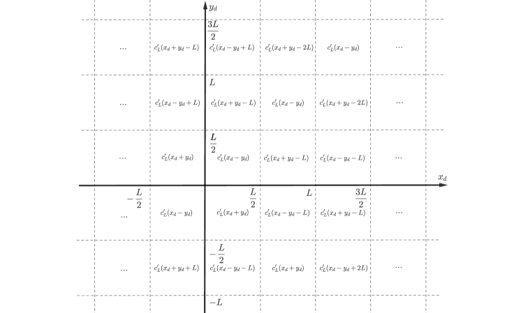
Figure 1. Piecewise definition of $c^{sym}_{L}(x,y)$ as a function of $x_{d},y_{d}$ (with the argument $x^{\prime}-y^{\prime}$ of $c^{\prime}_{L}$ suppressed)

It obviously inherits stationarity and periodicity in directions $i=1,\cdots,d-1$ from $c^{\prime}_{L}$ so that

$$c^{sym}_{L}(x,y) =c^{sym}_{L}(x+z^{\prime},y+z^{\prime})\quad\mbox{for}\;z^{\prime}\in\mathbb{R}^{d-1}\times\{0\},$$

(110) $$c^{sym}_{L}(x,y) =c^{sym}_{L}(x,y+Le_{i})\quad\mbox{for}\;i=1,\cdots,d.$$

Hence comparing $\langle\cdot\rangle_{L}$ to $\langle\cdot\rangle_{L}^{sym}$, we keep (full) periodicity, loose stationarity in direction $e_{d}$ but gain reflection symmetry in that direction. There are two derived symmetries that will play a role, namely

(111) $$c^{sym}_{L}(x,y) =c^{sym}_{L}(x,y+(L-2y_{d})e_{d}),$$

(112) $$c^{sym}_{L}(x,y) =c^{sym}_{L}(x+\tfrac{L}{2}e_{d},y+\tfrac{L}{2}e_{d}).$$

While (111) is an obvious combination of (108) and (109), (112) requires an argument, see Appendix B.1.

As for (7), we think of $\langle\cdot\rangle_{L}^{sym}$ as denoting also the push-forward of the Gaussian ensemble under $a=A(g)$. We now sample $a$ from $\langle\cdot\rangle_{L}^{sym}$. By construction, the scalar $a$ is not only $L$-periodic in every direction, cf. (110), but in addition even under reflection along the hyper planes $\{x_{d}=0\}$ and $\{x_{d}=\frac{L}{2}\}$, cf. (108), (111) and Figure 1. These invariances are transmitted to the solution $\phi_{i}^{(1)}$ of (2), and to the flux components $e_{i}\cdot a(\nabla\phi_{i}^{(1)}+e_{i})$ for any $i\neq d$. On the other hand, the flux component $e_{d}\cdot a(\nabla\phi_{1}^{(1)}+e_{1})$ is odd w. r. t.  these reflections and thus vanishes along these two hyper planes. Hence when it comes to $\phi^{(1)}_{1}$, the box $[-\frac{L}{2},\frac{L}{2}]^{d-1}\times[0,\frac{L}{2}]$ can be seen as an RVE with a flux boundary conditions in direction $e_{d}$ and periodic boundary conditions in directions $i=1,\cdots,d-1$. By the above reflection symmetry we have

$$\fint_{[-\frac{L}{2},\frac{L}{2}]^{d-1}\times[0,\frac{L}{2}]}e_{1}\cdot a(\nabla\phi_{1}^{(1)}+e_{1})=e_{1}\cdot\bar{a}e_{1},$$

where $\bar{a}$ is defined as in (3). We shall heuristically establish (4) in the form of

$$e_{1}\cdot(\langle\bar{a}\rangle_{L}^{sym}-a_{\rm hom})e_{1}=O(L^{-1}).$$

More precisely, we shall show that to leading order in $1-\lambda\ll 1$ and $L\gg 1$,

(113) $$e_{1}\cdot(\langle\bar{a}\rangle_{L}^{sym}-a_{\rm hom})e_{1}\approx-L^{-1}I\quad\mbox{with}\;I>0.$$

The sign of the leading-order correction $I$ is consistent with the following heuristics: The no-flux boundary conditions means that the current is restricted to the stripe $\mathbb{R}^{d-1}\times[0,\frac{L}{2}]$; for $d=2$ and as $L\downarrow 0$, the medium thus is close to a one-dimensional medium, for which one has the effective conductivity $\langle a^{-1}\rangle^{-1}\leq a_{\rm hom}$ (note that by statistical isotropy, also $a_{\rm hom}$ is scalar). This is also coherent with the usual observation that RVE approximations with Neumann boundary conditions estimate the actual homogenized coefficient by below, see [41].

As for $\langle\bar{a}\rangle_{L}$, we shall establish (113) by monitoring its $L$-derivative. More precisely, appealing to (41), we shall establish (113) in form of

(114) $$\frac{d}{dL}e_{1}\cdot(\langle\bar{a}\rangle_{L}^{sym}-\langle\bar{a}\rangle_{L})e_{1}\approx L^{-2}I.$$

The advantage of monitoring the difference between two ensembles is that we may use Price’s formula in a different, much less subtle, way than in Subsection 2.1. More precisely, in Appendix B.3, for a general $[0,L)^{d}$-periodic centered Gaussian ensemble $\langle\cdot\rangle_{L}$ we shall establish the formula

$$\frac{d}{dL}\langle e_{1}\cdot\bar{a}e_{1}\rangle_{L}=-L^{-d}\int_{[-\frac{L}{2},\frac{L}{2})^{d}}dx\int_{[-\frac{L}{2},\frac{L}{2})^{d}}dy$$

(115) $$\times\big{\langle}\big{(}a^{\prime}(\nabla\phi_{1}^{(1)}+e_{1})\big{)}(x)\cdot\nabla\nabla G^{per}(x,y)\cdot\big{(}a^{\prime}(\nabla\phi_{1}^{(1)}+e_{1})\big{)}(y)\big{\rangle}_{L}\frac{Dc_{L}}{\partial L}(x,y),$$

where the “material” derivative of the covariance function $c_{L}(x,y)$ is defined via

(116) $$\frac{Dc_{L}}{\partial L}(L\hat{x},L\hat{y})=\frac{d}{dL}\big{(}c_{L}(L\hat{x},L\hat{y})\big{)},$$

and where $G^{per}$ denotes the Green function associated with the operator $-\nabla\cdot a\nabla$ on the torus $[0,L)^{d}$, which is unambiguously defined in terms of its first and mixed derivatives. The present version of (4) also relies on

(117) $$\frac{Dc_{L}}{\partial L}(x,y)=0\quad\mbox{for}\;x=y.$$

Note that definition (116) implies

(118) $$\frac{Dc_{L}}{\partial L}\quad\mbox{is $[0,L)^{d}$-periodic in both arguments},$$

(119) $$\frac{Dc_{L}}{\partial L}=\frac{\partial c_{L}}{\partial L}+L^{-1}(x\cdot\nabla_{x}+y\cdot\nabla_{y})c_{L}.$$

Let us compare formula (4), which in the presence of stationarity simplifies (in the sense that $L^{-d}\int_{[-\frac{L}{2},\frac{L}{2})^{d}}dy$ is replaced by the evaluation at $y=0$), to (24). The main difference does not lie in the periodic setting (in view of (118), $\int_{[-\frac{L}{2},\frac{L}{2})^{d}}dx$ and $G^{per}$ can formally be replaced by $\int_{\mathbb{R}^{d}}dx$ and $G$, respectively), but in the convective contribution to (119), which is the generator of rescaling the space variables of $c$, and thus describes a rescaling of $a$. Indeed, this contribution vanishes after applying $\int_{\mathbb{R}^{d}}dx$ (only formally, since the integral does not converge absolutely) because the space average $\bar{a}e_{1}$ $=\lim_{R\uparrow\infty}\fint_{[0,R)^{d}}a(\nabla\phi_{1}^{(1)}+e_{1})$ is invariant under rescaling of $a$.

As in Subsection 2.4, in the small contrast regime, we have

$$\langle\big{(}a^{\prime}(\nabla\phi_{1}^{(1)}+e_{1})\big{)}(x)\cdot\nabla\nabla G^{per}(x,y)\cdot\big{(}a^{\prime}(\nabla\phi_{1}^{(1)}+e_{1})\big{)}(y)\big{\rangle}_{L}\approx-\partial_{1}^{2}G^{per}_{\rm hom}(x-y)\langle a^{\prime}(x)a^{\prime}(y)\rangle_{L},$$

so that (4) simplifies to

(120) $$\frac{d}{dL}\langle e_{1}\cdot\bar{a}e_{1}\rangle_{L} \approx L^{-d}\int_{[-\frac{L}{2},\frac{L}{2})^{d}}dx\int_{[-\frac{L}{2},\frac{L}{2})^{d}}dy\partial_{1}^{2}G^{per}_{\rm hom}(x-y)\langle a^{\prime}(x)a^{\prime}(y)\rangle_{L}\frac{Dc_{L}}{\partial L}(x,y).$$

We apply (120) to both $[0,L)^{d}$-periodic ensembles, $\langle\cdot\rangle_{L}^{sym}$ and $\langle\cdot\rangle_{L}$, which we may since (117) is satisfied (almost everywhere) for both: Indeed, by reflection symmetry (108) and periodicity (109), it is enough to consider $x\in\mathbb{R}^{d-1}\times[0,\frac{L}{2})$. Then for $|y-x|$ sufficiently small we have $c_{L}^{sym}(x,y)=c_{L}(x-y)$ by (107). By the finite-range assumption on $c$, this yields

$$c_{L}^{sym}(x,y)=c_{L}(x-y)=c(x-y)\quad\mbox{provided}\;|x-y|\;\mbox{is sufficiently small}\;\mbox{and}\;L\gg 1.$$

Hence we have for $y=x$ that $\frac{\partial}{\partial L}c_{L}^{sym}(x,y)$ $=\frac{\partial}{\partial L}c_{L}(0)$ $=0$ and $-\nabla_{y}c^{sym}_{L}(x,y)$ $=\nabla_{x}c^{sym}_{L}(x,y)$ $=\nabla c_{L}(0)$ $=0$. Introducing in addition the function ${\mathcal{A}}$ as in Subsection 2.4 for both $\langle a^{\prime}(x)a^{\prime}(y)\rangle_{L}$ $={\mathcal{A}}^{\prime}(c_{L}(x,y))$ and $\langle a^{\prime}(x)a^{\prime}(y)\rangle_{L}^{sym}$ $={\mathcal{A}}^{\prime}(c_{L}^{sym}(x,y))$, we obtain from (120)

(121) $$\frac{d}{dL}e_{1}\cdot(\langle\bar{a}\rangle_{L}^{sym}-\langle\bar{a}\rangle_{L})e_{1}\approx L^{-d}\int_{[-\frac{L}{2},\frac{L}{2})^{d}}dx\int_{[-\frac{L}{2},\frac{L}{2})^{d}}dy\partial_{1}^{2}G^{per}_{\rm hom}(x-y)\frac{D}{\partial L}\big{(}{\mathcal{A}}(c_{L}^{sym})-{\mathcal{A}}(c_{L})\big{)}(x,y).$$

There is a cancellation when considering the difference in (121): Indeed, by (107) and (108) (see also Figure 1) we have

$$c_{L}^{sym}(x,y)=c_{L}^{\prime}(x-y)\quad\mbox{provided}\;(x_{d},y_{d})\in[-\frac{L}{2},0]^{2}\cup[0,\frac{L}{2}]^{2}.$$

Likewise, we obtain from (9), (106) and the finite range of dependence assumption

$$c_{L}(x-y)=c_{L}^{\prime}(x-y)\quad\mbox{provided}\;(x_{d},y_{d})\in[-\frac{L}{2},0]^{2}\cup[0,\frac{L}{2}]^{2}.$$

Hence the integral in (121) reduces to $(x_{d},y_{d})$ $\in([-\tfrac{L}{2},0]\times[0,\tfrac{L}{2}])$ $\cup([0,\tfrac{L}{2}]\times[\tfrac{L}{2},0])$. Moreover, since the integrand in (120) is invariant under permuting $x$ and $y$, we obtain

$$\frac{d}{dL} e_{1}\cdot(\langle\bar{a}\rangle_{L}^{sym}-\langle\bar{a}\rangle_{L})e_{1}\approx 2L^{-d}\int_{[-\frac{L}{2},\frac{L}{2})^{d-1}\times[0,\frac{L}{2}]}dx\int_{[-\frac{L}{2},\frac{L}{2})^{d-1}\times[-\frac{L}{2},0]}dy$$

(122) $$\times\partial_{1}^{2}G^{per}_{\rm hom}(x-y)\frac{D}{\partial L}\big{(}{\mathcal{A}}(c_{L}^{sym})-{\mathcal{A}}(c_{L})\big{)}(x,y).$$

It follows from a combination of symmetries (108)&(109)&(112) that $c_{L}^{sym}$ is invariant under the inversion at $(\frac{L}{4},-\frac{L}{4})$ in the $(x_{d},y_{d})$ plane, that is,

(123) $$(x,y)\mapsto((x^{\prime},\tfrac{L}{2}-x_{d}),(y^{\prime},-\tfrac{L}{2}-y_{d})).$$

By stationarity, periodicity, and (243), $c_{L}$ has the same symmetry (123). By periodicity and radial symmetry, $(x,y)\mapsto\partial_{1}^{2}G^{per}_{\rm hom}(x-y)$ also has symmetry (123). Since the triangle in the $(x_{d},y_{d})$ plane

(124) $$\Delta:=\big{\{}x_{d}\geq 0,\quad y_{d}\leq 0,\quad x_{d}-y_{d}\leq\tfrac{L}{2}\big{\}}$$

is such that its (disjoint) union with its image under (123) renders the rectangle $[0,\frac{L}{2}]\times[-\frac{L}{2},0]$, (4) may be rewritten as

$$\frac{d}{dL} e_{1}\cdot(\langle\bar{a}\rangle_{L}^{sym}-\langle\bar{a}\rangle_{L})e_{1}\approx 4L^{-d}\int_{[-\frac{L}{2},\frac{L}{2})^{d-1}}dx^{\prime}\int_{[-\frac{L}{2},\frac{L}{2})^{d-1}}dy^{\prime}\int_{\Delta}dx_{d}dy_{d}$$

(125) $$\times\partial_{1}^{2}G^{per}_{\rm hom}(x-y)\frac{D}{\partial L}\big{(}{\mathcal{A}}(c_{L}^{sym})-{\mathcal{A}}(c_{L})\big{)}(x,y).$$

By the finite range assumption and for $L\gg 1$, we have (where for a stationary ensemble we identify $c(x,y)=c(x-y)$)

$$c_{L}(x,y)=c_{L}^{\prime}(x,y)\quad\mbox{provided}\;(x_{d},y_{d})\in\Delta,$$

so that in (4), we may replace $c_{L}$ by $c_{L}^{\prime}$. Likewise, by definition (107) and (108) (see also Figure 1) we have

$$c_{L}^{sym}(x,y)=c_{L}^{\prime}(x,y-2y_{d}e_{d})\quad\mbox{provided}\;(x_{d},y_{d})\in\Delta,$$

so that in (4), we may express $c_{L}^{sym}$ in terms of $c_{L}^{\prime}$. Since both ensembles $\langle\cdot\rangle_{L}^{\prime}$ and $\langle\cdot\rangle_{L}^{sym}$ are stationary in directions $i=1,\cdots,d-1$, (4) may be rewritten as

$$\frac{d}{dL} e_{1}\cdot(\langle\bar{a}\rangle_{L}^{sym}-\langle\bar{a}\rangle_{L})e_{1}\approx 4L^{-1}\int_{[-\frac{L}{2},\frac{L}{2}]^{d-1}}dx^{\prime}\int_{\Delta}dx_{d}dy_{d}\,\partial_{1}^{2}G^{per}_{\rm hom}(x-(0,y_{d}))$$

(126) $$\times\big{(}\frac{D}{\partial L}{\mathcal{A}}(c_{L}^{\prime})(x,(0,-y_{d}))-\frac{D}{\partial L}{\mathcal{A}}(c_{L}^{\prime})(x,(0,y_{d}))\big{)}.$$

By the finite range assumption and for $L\gg 1$, we have

$$c_{L}^{\prime}(x,(0,y_{d}))=c(x,(0,y_{d}))\quad\mbox{provided}\;x^{\prime}\in[-\tfrac{L}{2},\tfrac{L}{2}]^{d-1},$$

so that the material derivative in (4) reduces to the convective derivative; on stationary $c$’s, the convective derivative $L^{-1}(x\cdot\nabla_{x}+y\cdot\nabla_{y})$ acts as $L^{-1}z\cdot\nabla$ with $z=x-y$, and thus as the radial derivative $L^{-1}r\partial_{r}$ with $R=|z|$. Hence (4) takes the form

$$\frac{d}{dL} e_{1}\cdot(\langle\bar{a}\rangle_{L}^{sym}-\langle\bar{a}\rangle_{L})e_{1}\approx 4L^{-2}\int_{[-\frac{L}{2},\frac{L}{2}]^{d-1}}dx^{\prime}\int_{\Delta}dx_{d}dy_{d}\,\partial_{1}^{2}G^{per}_{\rm hom}(x^{\prime},x_{d}-y_{d})$$

(127) $$\times\big{(}(r\partial_{r}){\mathcal{A}}(c)(x^{\prime},x_{d}+y_{d})-(r\partial_{r}){\mathcal{A}}(c)(x^{\prime},x_{d}-y_{d})\big{)}.$$

We now proceed to a second (and last) approximation. Recall our assumption that $c$ is supported on the unit ball, hence the effective domain of integration in (4) is $|x^{\prime}|\leq 1$, next to $0\leq x_{d}-y_{d}\leq\frac{L}{2}$, cf. (124). In this range, we may approximate $G_{\rm hom}^{per}(x^{\prime},x_{d}-y_{d})$ by $G_{\rm hom}(x^{\prime},x_{d}-y_{d})$. After this substitution, we may neglect the restriction $x_{d}-y_{d}\leq\frac{L}{2}$. Hence (4) implies (114) where the $L$-independent quantity $I$ is defined via

$$I :=4\int_{\mathbb{R}^{d-1}}dx^{\prime}\int_{0}^{\infty}dx_{d}\int_{-\infty}^{0}dy_{d}\,\partial_{1}^{2}G_{\rm hom}(x^{\prime},x_{d}-y_{d})$$

(128) $$\times\big{(}(r\partial_{r}){\mathcal{A}}(c)(x^{\prime},x_{d}+y_{d})-(r\partial_{r}){\mathcal{A}}(c)(x^{\prime},x_{d}-y_{d})\big{)}.$$

In Appendix B.2, we compute this integral:

(129) $$I=\frac{32}{(d+1)(d-1)}\frac{|B_{1}^{\prime}|}{|\partial B_{1}|}\int_{0}^{\infty}dr{\mathcal{A}}(c),$$

where $B_{1}^{\prime}$ is the unit ball in $\mathbb{R}^{d-1}$. In particular, we have $I>0$, see Subsection 2.4 for the explanation why $\mathcal{A}$ is a nonnegative function (different from 0).

5. Proofs

5.1. Proof of Proposition 2: Limit $T\uparrow\infty$

The strategy of proof is as follows. First, we reorder the terms of the derivative of $\frac{d}{dL}\langle\xi^{*}\cdot\bar{a}_{T}\xi\rangle_{L}$ in order to make appear the “massive” analogue (that is, involving the massive operator $\frac{1}{T}-\nabla\cdot a\nabla$) of the r. h. s. of (64). For this first step, we essentially make rigorous the computations done in Section 2.2. Second, we systematically make use of the dominated convergence theorem to obtain the convergence of each term to its massless counterpart, yielding the formula (64).

Step 1. Formula for $\frac{d}{dL}\langle\xi^{*}\cdot\bar{a}_{T}\xi\rangle_{L}$. We establish the “massive analogue” of (64), namely

(130) $$\frac{d}{dL}\langle\xi^{*}\cdot\bar{a}_{T}\xi\rangle_{L}$$

$$=L^{-(d+1)}\int dz\xi^{*}\cdot\big{\langle}\overline{\Gamma}_{T/L^{2}ijmn}\,\big{(}-z_{m}Q^{(1)}_{Tij}(z)+Q^{(2)}_{Tijm}(z)\big{)}\big{\rangle}_{L}\xi\partial_{n}c(z)$$

$$+\int dz\xi^{*}\cdot\big{\langle}\epsilon^{(1)}_{TLijn}(z)Q^{(1)}_{Tij}(z)+\epsilon^{(2)}_{TLijmn}(z)Q^{(2)}_{Tijm}(z)\big{\rangle}_{L}\xi\partial_{n}c(z)$$

$$-\int dz(1-\eta_{L})(z)\big{\langle}(\nabla\phi^{*(1)}_{T}+\xi^{*})(0)\cdot a^{\prime}(0){\mathcal{E}}_{T}(0,z)a^{\prime}(z)(\nabla\phi^{(1)}_{T}+\xi)(z)\big{\rangle}_{L}\frac{\partial c_{L}}{\partial L}(z)$$

$$-\int dz\eta_{L}(z)\big{\langle}(\nabla\phi^{*(1)}_{T}+\xi^{*})(0)\cdot a^{\prime}(0)\nabla\nabla G_{T}(0,z)a^{\prime}(z)(\nabla\phi^{(1)}_{T}+\xi)(z)\big{\rangle}_{L}\frac{\partial c_{L}}{\partial L}(z)$$

$$+\frac{1}{2}\big{\langle}(\nabla\phi^{*(1)}_{T}+\xi^{*})\cdot a^{\prime\prime}(\nabla\phi^{(1)}_{T}+\xi)\big{\rangle}_{L}\frac{\partial c_{L}}{\partial L}(0),$$

where $\epsilon^{(1)}_{TLijn}$ & $\epsilon^{(2)}_{TLijlm}$ are defined as in (62) & (63) with $\bar{G}$ replaced by $\bar{G}_{T}$, where ${\mathcal{E}}_{T}$ is defined like in (60) with $G$ & $\bar{G}$ replaced by $G_{T}$ & $\bar{G}_{T}$ (but with non-massive first and second-order correctors), and where $Q^{(1)}_{T}$ & $Q^{(2)}_{T}$, which are quartic expressions in the correctors, are defined like in (36) & (37) with the first-order correctors $\phi^{(1)}$ & $\phi^{*(1)}$ (those linear in $\xi$ & $\xi^{*}$) replaced by their massive counterparts $\phi_{T}^{(1)}$ & $\phi_{T}^{*(1)}$ (but keeping the non-massive first and second order correctors $\phi_{i}^{(1)}$, $\phi_{j}^{*(1)}$, $\phi_{im}^{(2)}$, $\phi_{jm}^{*(2)}$). Recall that $\overline{\Gamma}_{T/L^{2}ijmn}$ is defined in (61).

The starting point is (59); the second r. h. s. term remains untouched and reappears as the last term in (130). Writing $\int dz$ $=\int dz(1-\eta_{L})(z)$ $+\int dz\eta_{L}(z)$, we split the first r. h. s. term in (59) into a far- and near-field part. The near-field part remains untouched and reappears as the previous to last term in (130). In the far-field part, we replace $\nabla\nabla G_{T}(0,z)$ according to the massive version of (60) by ${\mathcal{E}}_{T}(0,z)$ and terms involving $\bar{G}_{T}$. The contribution with ${\mathcal{E}}_{T}(0,z)$ reappears as the third r. h. s. term in (130). By the massive version of the definition (36) & (37) specified above, the terms involving $\bar{G}_{T}$ give rise to

$$-\int dz(1-\eta_{L})(z)\xi^{*}\cdot\big{(}-\big{\langle}\partial_{ij}\bar{G}_{T}(z)Q^{(1)}_{Tij}(z)\big{\rangle}_{L}+\big{\langle}\partial_{ijm}\bar{G}_{T}(z)Q^{(2)}_{Tijm}(z)\big{\rangle}_{L}\big{)}\xi\frac{\partial c_{L}}{\partial L}(z).$$

We now insert (25) and perform the resummation at the end of Subsection 2.1, which is based on the periodicity of $Q^{(1)}$ and $Q^{(2)}$ under $\langle\cdot\rangle_{L}$, and now is legitimate in view of the good decay properties of $\nabla\nabla G_{T}$ (see (57)) :

$$\int dz\sum_{k}k_{n}(1-\eta_{L})(z)\xi^{*}\cdot\big{(}-\big{\langle}\partial_{ij}\bar{G}_{T}(z+Lk)Q^{(1)}_{Tij}(z)\big{\rangle}_{L}+\big{\langle}\partial_{ijm}\bar{G}_{T}(z+Lk)Q^{(2)}_{Tijm}(z)\big{\rangle}_{L}\big{)}\xi\partial_{n}c(z).$$

Using that by parity, $\sum_{k}k_{n}\partial_{ij}\bar{G}_{T}(Lk)$ $=0$, we now appeal to the massive version of the definitions (62) & (63). This gives rise to the second r. h. s. of (130) and the leading order term

$$\int dz\xi^{*}\cdot\Big{\langle}\sum_{k}k_{n}\partial_{ijm}\bar{G}_{T}(Lk)\,\big{(}-z_{m}Q^{(1)}_{Tij}(z)+Q^{(2)}_{Tijm}(z)\big{)}\Big{\rangle}_{L}\xi\partial_{n}c(z).$$

It remains to insert the definition (61) and appeal to the scaling $\bar{G}_{T}(Lx)=L^{2-d}\bar{G}_{T/L^{2}}(x)$.

Step 2. Limit $T\uparrow\infty$. We now show that each term in (130) passes to the limit as $T\uparrow\infty$ and converges to its massless counterpart. To do so, we need to establish that this limit makes sense for each of the five r. h. s. terms of (130); in this task, the dominated convergence theorem is our main tool. Note that (67) and (68) hold uniformly in $T$, at the level of the massive quantities. Therefore, combined with the bounds and convergences of the massive quantities (54), (55), (56), (57) and Proposition 5, the second, third, fourth and fifth r. h. s. terms of (130) converge to their massless counterparts as $T\uparrow\infty$. Consequently, the subtle part is in the first r. h. s. term of (130), that we treat in details.

In the sequel, $L\geq 1$ is fixed. We prove that

(131) $$\begin{aligned} &\lim_{T\uparrow\infty}\int dz\big{\langle}\overline{\Gamma}_{T/L^{2}ijmn}\big{(}\xi^{*}\cdot Q^{(2)}_{Tijm}(z)\xi-z_{m}\xi^{*}\cdot Q^{(1)}_{Tij}(z)\xi\big{)}\big{\rangle}_{L}\partial_{n}c(z)\\ &=\int dz\big{\langle}\overline{\Gamma}_{ijmn}\big{(}\xi^{*}\cdot Q^{(2)}_{ijm}(z)\xi-z_{m}\xi^{*}\cdot Q^{(1)}_{ij}(z)\xi\big{)}\big{\rangle}_{L}\partial_{n}c(z).\end{aligned}$$

We claim that the only additional ingredient is the well-posedeness of $\overline{\Gamma}_{ijmn}:=\lim_{T\uparrow\infty}\overline{\Gamma}_{Tijmn}$ along with the bound

(132) $$\left|\overline{\Gamma}_{ijmn}\right|\leq\sup_{T\geq 1}|\overline{\Gamma}_{Tijmn}|\lesssim 1\text{ $\langle\cdot\rangle_{L}$-almost-surely},$$

where we recall (61)

$$\overline{\Gamma}_{Tijmn}:=\sum_{k\in\mathbb{Z}^{d}}k_{n}\partial_{ijm}\bar{G}_{T}(k).$$

Indeed, thanks to the assumption (10) on $c$, the bounds on the correctors (54), and (132), the integrand of the l. h. s integral in (131) is bounded (uniformly in $T$) by $(1+|z|)^{-d-2\alpha}$. We then conclude using the convergences (55) together with the Lebesgue convergence theorem.

Here comes the argument for (132). We fix a smooth compactly supported $\eta$ with $\eta=1$ on the unit cube $(-\frac{1}{2},\frac{1}{2})^{d}$ that we use it to split the lattice, which we interpret as a Riemann sum:

$$\sum_{k\not=0}k_{n}\partial_{ijm}\bar{G}_{T}(k)$$

$$=\int_{\mathbb{R}^{d}\backslash(-\frac{1}{2},\frac{1}{2})^{d}}dx\eta(x)x_{n}\partial_{ijm}\bar{G}_{T}(x)+\int dx(1-\eta)(x)x_{n}\partial_{ijm}\bar{G}_{T}(x)$$

(133) $$+\sum_{k\not=0}\big{(}k_{n}\partial_{ijm}\bar{G}_{T}(k)-\int_{k+(-\frac{1}{2},\frac{1}{2})^{d}}dxx_{n}\partial_{ijm}\bar{G}_{T}(x)\big{)}.$$

The first r. h. s. integral effectively extends over a compact subset of $\mathbb{R}^{d}\backslash\{0\}$ and thus obviously converges for $T\uparrow\infty$, thanks to (55). On the second r. h. s. integral in (5.1) we perform two integrations by parts:

$$\int dx(1-\eta)(x)x_{n}\partial_{ijm}\bar{G}_{T}(x)=\int dx\big{(}-\partial_{j}\eta(x)\delta_{mn}\partial_{i}\bar{G}_{T}(x)+\partial_{m}\eta(x)x_{n}\partial_{ij}\bar{G}_{T}(x)\big{)}.$$

Again, the r. h. s. integral effectively extends over a compact subset of $\mathbb{R}^{d}\backslash\{0\}$ and converges for $T\uparrow\infty$, thanks to (55). We finally turn to the last contribution in (5.1) where each summand has a limit $T\uparrow\infty$. This extends to the sum because of dominated convergence: Each summand is dominated, in absolute value, by the Lipschitz norm of $x\mapsto x_{n}\partial_{ijm}\bar{G}_{T}(x)$ on the translated cube $k+(-\frac{1}{2},\frac{1}{2})^{d}$, which by the uniform-in-$T$ decay of the derivatives of $\bar{G}_{T}$ (see (58)), gives an expression that is summable in $k\in\mathbb{Z}^{d}\backslash\{0\}$.

5.2. Proof of Lemma 1: Fluctuation estimates

As announced above, we show only (86) by closely following [39]. The only difference is that we appeal not only to the annealed Calderón-Zygmund estimates as in [39], but also to the annealed weighted estimates contained in Lemma 2.

For a deterministic and periodic vector field $h$, we consider the random variable of zero average

$$F:=\int_{[0,L)^{d}}h\cdot\nabla\phi_{ij}^{(2)}.$$

We employ on it the spectral gap inequality (cf. [39, Lem. 3.1]), which, combined with the Bochner estimate (assuming that $p\geq 2$), reads

(134) $$\langle|F|^{p}\rangle_{L}^{\frac{1}{p}}\lesssim\Big{(}\int_{[0,L)^{d}}\big{\langle}\big{|}\frac{\partial F}{\partial g}\big{|}^{p}\big{\rangle}_{L}^{\frac{2}{p}}\Big{)}^{\frac{1}{2}},$$

where $\frac{\partial F}{\partial g}=\frac{\partial F(g)}{\partial g(x)}$ is the Fréchet (or functional or vertical or Malliavin) derivative on $L^{2}([0,L)^{d})$ of $F$ w. r. t. $g$ defined by, for all periodic perturbation $\delta g\in L^{2}([0,L)^{d})$

$$\lim_{\varepsilon\downarrow 0}\frac{F(g+\varepsilon\delta g)-F(g)}{\varepsilon}:=\int_{[0,L)^{d}}dx\,\delta g(x)\frac{\partial F(g)}{\partial g(x)}.$$

(Since $L^{2}([0,L)^{d})$ is a Hilbert space, this Fréchet derivative is actually a gradient.) We split the proof into three steps. First, we establish that the Fréchet derivative of $F$ is given by

(135) $$\frac{\partial F}{\partial g}=\nabla v\cdot a^{\prime}(\nabla\phi^{(2)}_{ij}+\phi^{(1)}_{i}e_{j})-(\nabla w_{j}+ve_{j})\cdot a^{\prime}(\nabla\phi_{i}^{(1)}+e_{i}),$$

where $v$ and $w_{j}$ are defined through (140) and (142) below. Next, we show that the annealed estimates of Lemma 2 imply

(136) $$\big{(}\int_{[0,L)^{d}}\langle|\nabla v|^{2p}\rangle_{L}^{\frac{1}{p}}\big{)}^{\frac{1}{2}}\lesssim\big{(}\int_{[0,L)^{d}}|h|^{2}\big{)}^{\frac{1}{2}},$$

(137) $$\big{(}\int_{[0,L)^{d}}\langle|\nabla w_{j}+ve_{j}|^{2p}\rangle_{L}^{\frac{1}{p}}\big{)}^{\frac{1}{2}}\lesssim\big{(}\int_{[0,L)^{d}}|x|^{2}_{L}|h|^{2}\big{)}^{\frac{1}{2}},$$

where we recall that $|x|_{L}=\inf_{k\in\mathbb{Z}^{d}}|x+kL|$. Last, we insert (135) into (134) and we appeal to the Cauchy-Schwarz inequality (we also employ (11)), to the effect of

$$\langle|F|^{p}\rangle^{\frac{1}{p}} \lesssim\Big{(}\int_{[0,L)^{d}}\big{(}\langle|\nabla v^{2p}|\rangle^{\frac{1}{p}}\langle|\nabla\phi^{(2)}_{ij}+\phi^{(1)}_{i}e_{j}|^{2p}\rangle^{\frac{1}{p}}$$

$$\qquad\qquad+\langle|\nabla w_{j}+ve_{j}|^{2p}\rangle^{\frac{1}{p}}\langle|\nabla\phi_{i}^{(1)}+e_{i}|^{2p}\rangle^{\frac{1}{p}}\big{)}\Big{)}^{\frac{1}{2}}.$$

Invoking (76) and recalling (136) and (137) finally yields the desired estimate (86).

Step 1. Argument for (135). We give ourselves infinitesimal (periodic) perturbation $\delta g\in L^{2}([0,L)^{d})$ of $g$. In view of (2) and (29), it generates a perturbation $\delta\phi_{i}^{(1)}$ characterized by

(138) $$\nabla\cdot\big{(}a\nabla\delta\phi_{i}^{(1)}+\delta ga^{\prime}(\nabla\phi_{i}^{(1)}+e_{i})\big{)}=0\quad\mbox{and}\quad\fint_{[0,L)^{d}}\delta\phi_{i}^{(1)}=0.$$

In view of (31), this in turn generates the perturbation $\nabla\delta\phi_{ij}^{(2)}$ characterized by

(139) $$\begin{aligned} -\nabla\cdot\big{(}a(\nabla\delta\phi_{ij}^{(2)}+\delta\phi_{i}^{(1)}e_{j})+\delta ga^{\prime}(\nabla\phi^{(2)}_{ij}+\phi^{(1)}_{i}e_{j})\big{)}=Pe_{j}\cdot\big{(}a\nabla\delta\phi_{i}^{(1)}+\delta ga^{\prime}(\nabla\phi_{i}^{(1)}+e_{i})\big{)},\end{aligned}$$

where $P$ denotes the ($L^{2}$-orthogonal) projection onto functions of vanishing spatial mean, i. e. $Ph=h-\fint_{[0,L)^{d}}h$. The form of (139) motivates the introduction of the periodic function $v$ defined through

(140) $$\nabla\cdot(a^{*}\nabla v+h)=0\quad\mbox{and}\quad\fint_{[0,L)^{d}}v=0,$$

so that, by testing (140) with $\delta\phi^{(2)}_{ij}$ and (139) with $v$ , we obtain the representation for $\delta F:=\int_{[0,L)^{d}}h\cdot\nabla\delta\phi^{(2)}_{ij}$:

(141) $$\begin{aligned} \delta F=\int_{[0,L)^{d}}\Big{(}\nabla v\cdot\big{(}a\delta\phi_{i}^{(1)}e_{j}+\delta ga^{\prime}(\nabla\phi^{(2)}_{ij}+\phi^{(1)}_{i}e_{j})\big{)}-ve_{j}\cdot\big{(}a\nabla\delta\phi_{i}^{(1)}+\delta ga^{\prime}(\nabla\phi_{i}^{(1)}+e_{i})\big{)}\Big{)}.\end{aligned}$$

This in turn prompts the introduction of a second auxiliary periodic function $w_{j}$ of zero mean

(142) $$-\nabla\cdot a^{*}(\nabla w_{j}+ve_{j})=Pe_{j}\cdot a^{*}\nabla v,$$

so that by testing (138) with $w_{j}$ and (142) with $\delta\phi_{i}^{(1)}$, we may eliminate $\delta\phi_{i}^{(1)}$ in (141) and recover (135) in form of

$$\delta F=\int_{[0,L)^{d}}\delta g\Big{(}\nabla v\cdot a^{\prime}(\nabla\phi^{(2)}_{ij}+\phi^{(1)}_{i}e_{j})-(ve_{j}+\nabla w_{j})\cdot a^{\prime}(\nabla\phi_{i}^{(1)}+e_{i})\Big{)}.$$

Step 2. Argument for (136) and (137). Notice first that (136) is a direct consequence of Lemma 2 with weight $w=1$ applied to $v$ satisfying (140). Therefore, it remains to establish (137). In this perspective, we introduce the (gradient) field $h_{j}$ such that the r. h. s. of (142) reads $Pe_{j}\cdot a^{*}\nabla v$ $=\nabla\cdot h_{j}$. As a consequence of annealed unweighted estimates on $\nabla(-\nabla\cdot a^{*}\nabla)^{-1}\nabla\cdot$ (namely, Lemma 2 with weight $w=1$), we get

(143) $$\big{(}\int_{[0,L)^{d}}\langle|\nabla w_{j}|^{2p}\rangle_{L}^{\frac{1}{p}}\big{)}^{\frac{1}{2}}\lesssim\big{(}\int_{[0,L)^{d}}\langle|h_{j}|^{2p}+|v|^{2p}\rangle_{L}^{\frac{1}{p}}\big{)}^{\frac{1}{2}}.$$

We now claim the following annealed Hardy inequality:

(144) $$\big{(}\int_{[0,L)^{d}}\langle|v|^{2p}\rangle_{L}^{\frac{1}{p}}\big{)}^{\frac{1}{2}}\lesssim\big{(}\int_{[0,L)^{d}}|x|^{2}_{L}\langle|\nabla v|^{2p}\rangle_{L}^{\frac{1}{p}}\big{)}^{\frac{1}{2}}.$$

As a consequence of annealed weighted estimates on $\nabla(-\nabla\cdot a^{*}\nabla)^{-1}\nabla\cdot$ (namely, Lemma 2 with weight $w=|\cdot|^{2}_{L}$) applied to (140), we have

(145) $$\big{(}\int_{[0,L)^{d}}|x|^{2}_{L}\langle|\nabla v|^{2p}\rangle_{L}^{\frac{1}{p}}\big{)}^{\frac{1}{2}}\lesssim\big{(}\int_{[0,L)^{d}}|x|^{2}_{L}|h|^{2}\big{)}^{\frac{1}{2}},$$

and therefore, by (144), there holds

(146) $$\big{(}\int_{[0,L)^{d}}\langle|v|^{2p}\rangle_{L}^{\frac{1}{p}}\big{)}^{\frac{1}{2}}\lesssim\big{(}\int_{[0,L)^{d}}|x|^{2}_{L}|h|^{2}\big{)}^{\frac{1}{2}}.$$

Moreover, by the annealed weighted estimates on $\nabla^{2}(-\triangle)^{-1}$ [47, Theorem 7.1], we obtain

$$\big{(}\int_{[0,L)^{d}}|x|^{2}_{L}\langle|\nabla h_{j}|^{2p}\rangle_{L}^{\frac{1}{p}}\big{)}^{\frac{1}{2}}\lesssim\big{(}\int_{[0,L)^{d}}|x|^{2}_{L}\langle|\nabla v|^{2p}\rangle_{L}^{\frac{1}{p}}\big{)}^{\frac{1}{2}}.$$

Combining it with the Hardy inequality (144) for $h_{j}$ and with (145) yields

$$\big{(}\int_{[0,L)^{d}}\langle|h_{j}|^{2p}\rangle_{L}^{\frac{1}{p}}\big{)}^{\frac{1}{2}}\lesssim\big{(}\int_{[0,L)^{d}}|x|^{2}_{L}|h|^{2}\big{)}^{\frac{1}{2}}$$

Inserting this and (146) into (143), and employing once more (146) in the triangle inequality gives (137).

Step 3. Argument for (144). W. l. o. g. we may assume that $L=1$, and we consider random periodic functions of vanishing average $v$. The annealed Hardy inequality (144) relies on three ingredients. First, if $\langle|u|^{2p}\rangle^{\frac{1}{p}}$ is compactly supported, we have

(147) $$\int\langle|u|^{2p}\rangle^{\frac{1}{p}}\lesssim\int|x|^{2}\langle|\nabla u|^{2p}\rangle^{\frac{1}{p}}.$$

Next, for $\Omega:=[-\frac{1}{2},\frac{1}{2})^{d}\backslash[-\frac{1}{4},\frac{1}{4})^{d}$, the following annealed Poincaré estimate holds:

(148) $$\Big{(}\int_{\Omega}\langle|v|^{2p}\rangle^{\frac{1}{p}}\Big{)}^{\frac{1}{2}}\lesssim\Big{(}\int_{\Omega}\langle|\nabla v|^{2p}\rangle^{\frac{1}{p}}\Big{)}^{\frac{1}{2}}+\int_{\Omega}\langle|v|^{2p}\rangle^{\frac{1}{2p}}.$$

Last, we make use of an annealed Poincaré-Wirtinger estimate

(149) $$\int_{[-\small\frac{1}{2},\small\frac{1}{2})^{d}}\langle|v|^{2p}\rangle^{\frac{1}{2p}}\lesssim\int_{[-\small\frac{1}{2},\small\frac{1}{2})^{d}}\langle|\nabla v|^{2p}\rangle^{\frac{1}{2p}}.$$

Using (147) for $u:=\eta v$ where $\eta$ is a cut-off function of $[-\small\frac{1}{2},\small\frac{1}{2})^{d}$ into $[-\small\frac{3}{4},\small\frac{3}{4})^{d}$, we have by periodicity of $v$

$$\int_{[-\small\frac{1}{2},\small\frac{1}{2})^{d}}\langle|v|^{2p}\rangle^{\frac{1}{p}}\lesssim\int_{[-\small\frac{1}{2},\small\frac{1}{2})^{d}}|x|^{2}_{1}\langle|\nabla v|^{2p}\rangle^{\frac{1}{p}}+\int_{\Omega}\langle|v|^{2p}\rangle^{\frac{1}{p}},$$

Inserting (148) and then (149) into the above estimate yields

(150) $$\int_{[-\small\frac{1}{2},\small\frac{1}{2})^{d}}\langle|v|^{2p}\rangle^{\frac{1}{p}} \lesssim\int_{[-\small\frac{1}{2},\small\frac{1}{2})^{d}}|x|^{2}_{1}\langle|\nabla v|^{2p}\rangle^{\frac{1}{p}}+\Big{(}\int_{[-\small\frac{1}{2},\small\frac{1}{2})^{d}}\langle|\nabla v|^{2p}\rangle^{\frac{1}{2p}}\Big{)}^{2}.$$

Since $d>2$, we may employ the Cauchy-Schwarz inequality to get

$$\Big{(}\int_{[-\small\frac{1}{2},\small\frac{1}{2})^{d}}\langle|\nabla v|^{2p}\rangle^{\frac{1}{2p}}\Big{)}^{2} \leq\int_{[-\small\frac{1}{2},\small\frac{1}{2})^{d}}|x|^{2}_{1}\langle|\nabla v|^{2p}\rangle^{\frac{1}{p}}\int_{[-\small\frac{1}{2},\small\frac{1}{2})^{d}}|x|^{-2}_{1}$$

$$\lesssim\int_{[-\small\frac{1}{2},\small\frac{1}{2})^{d}}|x|^{2}_{1}\langle|\nabla v|^{2p}\rangle^{\frac{1}{p}}.$$

Inserting this into (150) yields the desired (144) (noting that by periodicity, we can replace $[-\tfrac{1}{2},\tfrac{1}{2})$ by $[0,1)^{d}$).

We now establish successively (147), (148), and (149). First, (147) comes by applying the following Hardy inequality for compactly supported functions $\phi$ (see [6, Theorem 1.2.8] with $p=2$ and $V=|x|^{2}$):

$$\int_{\mathbb{R}^{d}}|\phi|^{2}\lesssim\int_{\mathbb{R}^{d}}|x|^{2}|\nabla\phi|^{2},$$

to $\phi\rightsquigarrow\langle|u|^{2p}\rangle^{\frac{1}{2p}}$, and noticing that by the Hölder inequality with exponents $(\frac{2p}{2p-1},2p)$

$$|\nabla\langle|u|^{2p}\rangle^{\frac{1}{2p}}|=|\langle|u|^{2p}\rangle^{\frac{1}{2p}-1}\langle|u|^{2p-1}\nabla|u|\rangle|\leq\langle|\nabla u|^{2p}\rangle^{\frac{1}{2p}}.$$

Similarly, we get (148) from the usual Poincaré inequality applied to the function $\langle|v|^{2p}\rangle^{\frac{1}{2p}}$. Last, we get (149) by recalling that $v$ is periodic of vanishing average in $[-\small\frac{1}{2},\small\frac{1}{2})^{d}$, so that

$$\int_{[-\small\frac{1}{2},\small\frac{1}{2})^{d}}\langle|v|^{2p}\rangle^{\frac{1}{2p}}=\int_{[-\small\frac{1}{2},\small\frac{1}{2})^{d}}\big{\langle}\big{|}v-\int_{[-\small\frac{1}{2},\small\frac{1}{2})^{d}}v\big{|}^{2p}\big{\rangle}^{\frac{1}{2p}}$$

$$\qquad\leq\int_{[-\small\frac{1}{2},\small\frac{1}{2})^{d}}dx\int_{[-\small\frac{1}{2},\small\frac{1}{2})^{d}}dy\langle|v(x)-v(x+y)|^{2p}\rangle^{\frac{1}{2p}}$$

$$\qquad\leq\int_{[-\small\frac{1}{2},\small\frac{1}{2})^{d}}dx\int_{[-\small\frac{1}{2},\small\frac{1}{2})^{d}}dy\big{\langle}\big{(}|y|\int_{0}^{1}ds|\nabla v(x+sy)|\big{)}^{2p}\big{\rangle}^{\frac{1}{2p}}$$

$$\qquad\lesssim\int_{[-\small\frac{1}{2},\small\frac{1}{2})^{d}}dx\int_{[-\small\frac{1}{2},\small\frac{1}{2})^{d}}dz\langle|\nabla v(z)|^{2p}\rangle^{\frac{1}{2p}}=\int_{[-\small\frac{1}{2},\small\frac{1}{2})^{d}}\langle|\nabla v|^{2p}\rangle^{\frac{1}{2p}}.$$

5.3. Proof of Corollary 1: Limit $L\uparrow\infty$

In view of (2) and (29), we may consider the field $\phi^{(1)}$ as a function of $g$, provided the latter is periodic. The same applies to $\phi^{(2)}$, cf. (31), provided we make it unique through

(151) $$\phi^{(2)}_{ij}(0)=0.$$

We will monitor the joint distribution of the triplet of fields $(g,\phi^{(1)}_{i}(g),\phi^{(2)}_{ij}(g))$ under $\langle\cdot\rangle_{L}$. This amounts to the push-forward $\langle\cdot\rangle_{L,ext}$ of $\langle\cdot\rangle_{L}$ under the map $g\mapsto(g,\phi^{(1)}_{i}(g),\phi^{(2)}_{ij}(g))$, which we denote by $(\text{Id},\phi^{(1)}_{i},\phi^{(2)}_{ij})$:

(152) $$\langle\cdot\rangle_{L,ext}:=(\text{Id},\phi^{(1)}_{i},\phi^{(2)}_{ij})\#\langle\cdot\rangle_{L};$$

the index “ext” hints to the fact that $\langle\cdot\rangle_{L,ext}$ is an extension of $\langle\cdot\rangle_{L}$ in the sense that the latter is the marginal of the former w. r. t. the first component. As will become apparent in Step 1, $\langle\cdot\rangle_{L,ext}$ is a probability measure on the product space $\mathcal{C}^{0,\alpha,\beta}\times\mathcal{C}^{1,\alpha,\beta}\times\mathcal{C}^{1,\alpha,\beta}$, provided $\alpha\in(0,1)$ and $\beta\in(\frac{1}{2},\infty)$, where $\mathcal{C}^{n,\alpha,\beta}$ denotes the space of functions that are locally in $\mathcal{C}^{n,\alpha}$ but are allowed to grow at rate $\beta$:

$$\mathcal{C}^{n,\alpha,\beta}:=\{\,\phi\colon\mathbb{R}^{d}\rightarrow\mathbb{R}\,|\,\|\phi\|_{n,\alpha,\beta}:=\sup_{x\in\mathbb{R}^{d}}(1+|x|)^{-\beta}\|\phi\|_{C^{n,\alpha}(B_{1}(x))}<\infty\}.$$

On the one hand, this norm is weak enough so that Proposition 3 implies that the family $\{\langle\cdot\rangle_{L,ext}\}_{L\uparrow\infty}$ is tight, see Step 1. On the other hand, it is (obviously) strong enough so that $q$, $Q^{(1)}_{ij}(z)$ and $Q^{(2)}_{ijm}(z)$ are continuous functions of $g$, cf. (16), (36) and (37), which will imply part $iii)$ of the corollary. In Step 2, we show that any (weak) limit $\langle\cdot\rangle_{ext}$ is stationary, satisfies the moment bounds of Corollary 1, and is supported on fields that satisfy the relations of Corollary 1. In Step 3, we identify the first marginal of $\langle\cdot\rangle_{ext}$ with our whole-space ensemble $\langle\cdot\rangle$. In Step 4, we construct $\phi^{(1)}_{i}$ and $\phi^{(2)}_{ij}$, now only defined almost surely, satisfying the requirements of Corollary 1. Finally, in Step 5, we argue that $\langle\cdot\rangle_{ext}$ is the push-forward of the whole-space ensemble $\langle\cdot\rangle$ under the map $(\text{Id},\phi^{(1)}_{i},\phi^{(2)}_{ij})$. In the following, we drop the indices $i$ and $j$.

Step 1. Compactness result. We show that Proposition 3 implies for $\alpha\in(0,1)$, $\beta\in(\frac{1}{2},\infty)$, and $p<\infty$

(153) $$\sup_{L\geq 1}\langle(\|\text{Id}\|_{0,\alpha,\beta}+\|(\phi^{(1)},\phi^{(2)})\|_{1,\alpha,\beta})^{p}\rangle_{L}<\infty.$$

We combine this with the compact embedding $\mathcal{C}^{n,\alpha^{\prime},\beta^{\prime}}\subset\mathcal{C}^{n,\alpha,\beta}$ for $\alpha<\alpha^{\prime}$ and $\beta^{\prime}<\beta$, which is a consequence of Arzelà-Ascoli’s theorem. This implies by Prohorov’s theorem [13, Theorem 3.8.4] that there exists a probability measure $\langle\cdot\rangle_{ext}$ on $\mathcal{C}^{0,\alpha^{\prime},\beta^{\prime}}\times\mathcal{C}^{1,\alpha^{\prime},\beta^{\prime}}\times\mathcal{C}^{1,\alpha^{\prime},\beta^{\prime}}$ such that, up to a subsequence that we do not relabel,

(154) $$\langle\cdot\rangle_{L,ext}\underset{L\uparrow\infty}{\rightharpoonup}\langle\cdot\rangle_{ext}.$$

We argue for (153). Since the balls $\{B_{1}(x)\}_{x\in\frac{1}{\sqrt{d}}\mathbb{Z}^{d}}$ cover $\mathbb{R}^{d}$, we have by a union bound argument

$$\big{\langle}\big{(}\|g\|_{0,\alpha,\beta}+\|(\phi^{(1)},\phi^{(2)})\|_{1,\alpha,\beta}\big{)}^{p}\big{\rangle}_{L} \lesssim\big{\langle}\big{(}\sup_{x\in\frac{1}{\sqrt{d}}\mathbb{Z}^{d}}(1+|x|)^{-\beta}(\|g\|_{C^{0,\alpha}(B_{1}(x))}+\|(\phi^{(1)},\phi^{(2)})\|_{C^{1,\alpha}(B_{1}(x))})\big{)}^{p}\big{\rangle}_{L}$$

(155) $$\leq\sum_{x\in\frac{1}{\sqrt{d}}\mathbb{Z}^{d}}(1+|x|)^{-p\beta}\langle(\|g\|_{C^{0,\alpha}(B_{1}(x))}+\|(\phi^{(1)},\phi^{(2)})\|_{C^{1,\alpha}(B_{1}(x))})^{p}\rangle_{L}.$$

By local Schauder theory we obtain from (2) and (31)

$$\|\phi^{(1)}\|_{C^{1,\alpha}(B_{1}(x))} \lesssim C(\|a\|_{C^{0,\alpha}(B_{2}(x))})\Big{(}1+\Big{(}\int_{B_{2}(x)}|\phi^{(1)}|^{2}\Big{)}^{\frac{1}{2}}\Big{)},$$

$$\|\phi^{(2)}\|_{C^{1,\alpha}(B_{1}(x))} \lesssim C(\|a\|_{C^{0,\alpha}(B_{2}(x))})\Big{(}\|\phi^{(1)}\|_{C^{1,\alpha}(B_{2}(x))}+\Big{(}\int_{B_{2}(x)}|\phi^{(2)}|^{2}\Big{)}^{\frac{1}{2}}\Big{)}$$

with an at most polynomial dependence of the constant on $\|a\|_{C^{0,\alpha}(B_{2}(x))}$. By (13) this yields

(156) $$\big{\langle}\big{(}\|g\|_{C^{0,\alpha}(B_{1}(x))}+\|(\phi^{(1)},\phi^{(2)})\|_{C^{1,\alpha}(B_{1}(x))}\big{)}^{p}\big{\rangle}_{L}^{\frac{1}{p}}\lesssim_{p,p^{\prime}}1+\int_{B_{2}(x)}\langle|(\phi^{(1)},\phi^{(2)})|^{p^{\prime}}\rangle_{L}^{\frac{1}{p^{\prime}}},$$

provided $p<p^{\prime}$. By Proposition 3 $i)$ for $\phi^{(1)}$ and by $iv)$ for $\phi^{(2)}$ together with (151), we have that the r. h. s. of (156) is estimated by $(1+|x|)^{\frac{1}{2}}$. Hence the summand on the r. h. s. of (5.3) is estimated by $(1+|x|)^{-p(\beta-\frac{1}{2})}$, which is summable provided $p>\frac{d}{\beta-\frac{1}{2}}$. The remaining range is then obtained by Jensen’s inequality.

Step 2. Stationarity, moment bounds, and PDE-constrained support of $\langle\cdot\rangle_{ext}$. Here and in the sequel, we denote by $(g,\phi,\psi)\in{\mathcal{C}}_{\alpha,\beta}^{0}\times{\mathcal{C}}_{\alpha,\beta}^{1}\times{\mathcal{C}}_{\alpha,\beta}^{1}$ the integration variables of $\langle\cdot\rangle_{L,ext}$ and its limit $\langle\cdot\rangle_{ext}$. First, because ${\mathcal{C}}_{\alpha,\beta}^{1}\ni\psi\mapsto\psi^{2}(0)$ is continuous, (151) is preserved under (154):

(157) $$\psi(0)=0\quad\text{for $\langle\cdot\rangle_{ext}$-a.~{}e. $\psi$}.$$

Next, note that $\phi^{(1)}$ and $\nabla\phi^{(2)}$ are shift-covariant (the anchoring (151) of $\phi^{(2)}$ does not admit shift-covariance, but does not affect the shift-covariance of $\nabla\phi^{(2)}$) and $\langle\cdot\rangle_{L}$ is stationary. Hence, we may introduce the push-forward of $\langle\cdot\rangle_{L,ext}$ under the map $(g,\phi,\psi)\mapsto(g,\phi,\nabla\psi)$, which we call $(\text{Id},\text{Id},\nabla)$ and which is stationary, a linear constraint that is preserved under the weak convergence (154):

(158) $$(\text{Id},\text{Id},\nabla)\#\langle\cdot\rangle_{ext}\text{ is stationary.}$$

We now turn to the estimates of Proposition 3. Clearly, the bounds (76), the second bound in (77) for any compactly supported function $\eta$ and (78) are preserved under (154):

(159) $$\langle|\nabla\phi|^{p}+|\phi|^{p}+|\nabla\psi|^{p}\rangle_{ext}\lesssim_{p}1,\quad\big{\langle}\big{|}\int\eta\phi\big{|}^{p}\big{\rangle}_{ext}^{\frac{1}{p}}\lesssim_{p}\big{(}\int|\eta|^{\frac{2d}{d+2}}\big{)}^{\frac{d+2}{2d}},\quad\mbox{and}\quad\langle|\psi(z)|^{p}\rangle_{ext}^{\frac{1}{p}}\lesssim_{p}\mu^{(2)}_{d}(|z|).$$

Finally, from the weak convergence (154), the definition of $\overline{a}$ in (3) together with the stationarity of $\langle\cdot\rangle_{L}$ in form of $\langle\overline{a}\rangle_{L}=\langle a(\nabla\phi^{(1)}+e_{i})(0)\rangle_{L}$ and the decay of averages (77) for the flux (applied with $\eta=L^{-d}\mathds{1}_{[0,L)^{d}}$), one has

$$\langle\overline{a}\rangle_{L}\underset{L\uparrow\infty}{\rightarrow}\langle a(\nabla\phi+e_{i})(0)\rangle_{ext}\quad\mbox{and}\quad\langle|\overline{a}-\langle\overline{a}\rangle_{L}|\rangle_{L}\lesssim L^{-\frac{d}{2}},$$

so that $\langle|\overline{a}-\langle a(\nabla\phi+e_{i})\rangle_{ext}|\rangle_{L}\underset{L\uparrow\infty}{\rightarrow}0$. Therefore, introducing the notation $a_{\text{hom},ext}:=\langle a(\nabla\phi+e_{i})(0)\rangle_{ext}$, we obtain under the weak convergence (154) that the equations (2) and (31), when tested against smooth compactly supported functions, are preserved in the sense that

(160) $$\nabla\cdot a(\nabla\phi+e_{i})=0\quad\text{and}\quad-\nabla\cdot a(\nabla\psi+\phi e_{j})=e_{j}\cdot(a(\nabla\phi+e_{i})-a_{\text{hom},ext}e_{i})\quad\mbox{for}\;\langle\cdot\rangle_{ext}\mbox{-a.~{}e.}\;(g,\phi,\psi).$$

Step 3. Identification of the first marginal of $\langle\cdot\rangle_{ext}$. More precisely, we show that is given by $\langle\cdot\rangle$. By the definition (152), the first marginal of $\langle\cdot\rangle_{L,ext}$ is the Gaussian measure $\langle\cdot\rangle_{L}$. By (154), the sequence $\{\langle\cdot\rangle_{L}\}_{L\uparrow\infty}$ of Gaussian measures is tight on $\mathcal{C}^{0,\alpha,\beta}$. By [13, Corollary 3.8.5], it is thus enough to prove the weak convergence of $\langle\cdot\rangle_{L}$ to $\langle\cdot\rangle$ on squares of bounded linear forms:

(161) $$\lim_{L\uparrow\infty}\langle\ell^{2}\rangle_{L}=\langle\ell^{2}\rangle\quad\text{for all $\ell\in(\mathcal{C}^{0,\alpha,\beta})^{*}$.}$$

By density and tightness, it is enough to check (161) for linear forms $\ell$ of the form $g\mapsto\int\zeta g$ for an arbitrary Schwartz function $\zeta$. The definition (9) of $c_{L}$ can also be stated in terms of the (distributional) Fourier transform of the (periodic) $c_{L}$ as

$${\mathcal{F}}c_{L}=\big{(}\frac{2\pi}{L}\big{)}^{d}\sum_{q\in\frac{2\pi}{L}\mathbb{Z}^{d}}{\mathcal{F}}c(q)\delta(\cdot-q).$$

Hence the l. h. s. of (161) assumes the form of a Riemann sum:

$$\langle\ell^{2}\rangle_{L}=\big{(}\frac{2\pi}{L}\big{)}^{d}\sum_{q\in\frac{2\pi}{L}\mathbb{Z}^{d}}\mathcal{F}c(q)|\mathcal{F}\zeta(q)|^{2}.$$

Since by Assumption 1 in form of the integrability of $c$, see (12), $\mathcal{F}c$ is continuous, we obtain (161):

$$\lim_{L\uparrow\infty}\langle\ell^{2}\rangle_{L}=\int\mathcal{F}c|\mathcal{F}\zeta|^{2}=\langle\ell^{2}\rangle.$$

Step 4. Construction of $\phi^{(1)}$ and $\phi^{(2)}$. We show that there exist $\phi^{(1)}$ and $\phi^{(2)}$ satisfying Corollary 1 $i)$ and $ii)$ respectively. We construct these random variables via disintegration of the measure $\langle\cdot\rangle_{ext}$ with respect to its first marginal $\langle\cdot\rangle$, which amounts to conditional expectation w. r. t. $g$. By [45, Theorem 6.4] there exists a family of measures $\{\langle\cdot|g\rangle_{ext}\}_{g\in\mathcal{C}^{0}_{\alpha,\beta}}$ on $\mathcal{C}^{1}_{\alpha,\beta}\times\mathcal{C}^{1}_{\alpha,\beta}$ such that for all $\langle\cdot\rangle_{ext}$-integrable functions $F$,

$$\langle F\rangle_{ext}=\langle\langle F|g\rangle_{ext}\rangle.$$

We now define the $\langle\cdot\rangle$-integrable functions $\phi^{(1)}$ and $\phi^{(2)}$ through conditional expectation

(162) $$\phi^{(1)}(g):=\langle\phi|g\rangle_{ext}\quad\mbox{and}\quad\phi^{(2)}(g):=\langle\psi|g\rangle_{ext}\quad\mbox{for all}\;g\in\mathcal{C}^{0}_{\alpha,\beta}$$

and verify that they satisfy all the requirements of Corollary 1 $i)$ and $ii)$. Since the conditioning w. r. t. $g$ commutes with the multiplication by $a=A(g)$, the linear equations (160) are preserved and give rise to (90) and (92). It is easy to check that the stationarity (158) translates into shift-covariance of $\phi^{(1)}$ and $\nabla\phi^{(2)}$. It follows from (157), via Jensen’s inequality applied to the conditional expectation, that $\phi^{(1)}$ and $\phi^{(2)}$ satisfy the moment bounds of Corollary 1 $i)$ and $ii)$, and also the decay bound (89) and the growth bound (91).

Step 5. Identification of $\langle\cdot\rangle_{ext}$. We now establish

$$\langle\cdot\rangle_{ext}=(\text{Id},\phi^{(1)},\phi^{(2)})\#\langle\cdot\rangle.$$

by showing

(163) $$u^{(1)}:=\phi-\phi^{(1)}(g)=0\quad\mbox{and}\quad u^{(2)}:=\psi-\phi^{(2)}(g)=0\quad\mbox{for}\;\langle\cdot\rangle_{ext}-\mbox{a.~{}e.}\;(g,\phi,\psi).$$

By (90) and (160), we have $-\nabla\cdot a\nabla u^{(1)}=0$ $\langle\cdot\rangle_{ext}$-a. s.. By Caccioppoli’s inequality we thus obtain

$$\fint_{B_{R}}|\nabla u^{(1)}|^{2}\lesssim\frac{1}{R^{2}}\fint_{B_{2R}}|u^{(1)}|^{2}\quad\mbox{for all}\;R<\infty.$$

Taking the expectation $\langle\cdot\rangle_{ext}$ and using the shift-covariance of $\phi^{(1)}$ and (158) this implies

$$\langle|\nabla u^{(1)}|^{2}\rangle_{ext}\lesssim\frac{1}{R^{2}}\langle|u^{(1)}|^{2}\rangle_{ext}\quad\mbox{for all}\;R<\infty.$$

Letting $R\uparrow\infty$ while appealing to (76) and (159) yields $\nabla u^{(1)}=0$. We now use (89) and the associated property in (159), for the averaging function $\eta=R^{-d}\mathds{1}_{B_{R}}$. Because of $\frac{2d}{d+2}>1$ this yields $\lim_{R\uparrow\infty}\langle|\fint_{B_{R}}u^{(1)}|^{2}\rangle_{ext}=0$. Hence we obtain the first claim of (163). Note that this implies in particular $a_{\text{hom},ext}=a_{\text{hom}}$, namely the first claim of Corollary 1 $iii)$.

It now follows from (92) and (160) that $-\nabla\cdot a\nabla u^{(2)}=0$ $\langle\cdot\rangle_{ext}$-a. s.. Starting again with Caccioppoli’s inequality, followed by the combination of shift-covariance of $\nabla\phi^{(2)}$ and (158), finally followed by the combination of (91) and (159), we obtain

$$\langle|\nabla u^{(2)}|^{2}\rangle_{ext}\lesssim\frac{1}{R^{2}}\fint_{B_{2R}}dz\langle|u^{(2)}(z)|^{2}\rangle_{ext}\lesssim\big{(}\frac{\mu^{(2)}_{d}(R)}{R}\big{)}^{2}\quad\mbox{for all}\;R<\infty.$$

Letting $R\uparrow\infty$ we conclude $\nabla u^{(2)}=0$. Using once more the combination of (91) and (159), this time for $z=0$, we find $u^{(2)}(0)=0$, which gives the second claim of (163). The same argument shows that there is at most one pair $(\phi^{(1)},\phi^{(2)})$ of random variables satisfying the properties of Corollary 1 $i)$ and $ii)$. Therefore, $\langle\cdot\rangle_{ext}$ is unique and thus the limit of $\langle\cdot\rangle_{L,ext}$ for the entire sequence $L\uparrow\infty$.

5.4. Proof of Lemma 4: Improved Caccioppoli inequality

By scaling, it is enough to consider $R=2$; we fix a smooth cut-off function $\eta$ for $B_{1}$ in $B_{2}$. Our starting point is the following localized version of a standard $L^{2}$-based interpolation estimate, with $n\in\mathbb{N}$ to be fixed later, which we take from the proof of [10, Lemma 4]:

(164) $$\int(\eta^{4n}\triangle^{2n}w)^{2}\lesssim\big{(}\int|\eta^{4n+1}\nabla\triangle^{2n}w|^{2}\big{)}^{\frac{4n}{4n+1}}\big{(}\int w^{2}\big{)}^{\frac{1}{4n+1}}+\int w^{2}.$$

We apply it to $w\in H^{2n}_{0}(B_{2})$ (as usual, $H^{2n}_{0}(B_{2})$ denotes the closure of $C^{\infty}_{0}(B_{2})$ w. r. t. the $H^{2n}(B_{2})$-norm) that (weakly) solves

(165) $$\triangle^{2n}w=u\quad\mbox{in}\quad B_{2}.$$

We construct $w$ with help of the Riesz representation theorem, so that we automatically have

(166) $$\int uw=\int(\triangle^{n}w)^{2}\sim\int|\nabla^{2n}w|^{2}\gtrsim\int w^{2},$$

where we used higher-order $L^{2}$-regularity and a higher-order Poincaré estimate. We obtain from inserting (165) into (164)

$$\int(\eta^{4n}u)^{2}\lesssim\big{(}\int|\eta^{4n+1}\nabla u|^{2}\big{)}^{\frac{4n}{4n+1}}\big{(}\int w^{2}\big{)}^{\frac{1}{4n+1}}+\int w^{2}.$$

Combining this with Caccioppoli’s estimate $\int|\eta^{4n+1}\nabla u|^{2}\lesssim\int(\eta^{4n}u)^{2}$ and Young’s inequality, we obtain

$$\int(\eta^{4n}u)^{2}\lesssim\int w^{2},$$

so that, by the choice of $\eta$, we deduce

(167) $$\int_{B_{1}}|\nabla u|^{2}\leq\int(\eta^{4n}u)^{2}\lesssim\int w^{2}.$$

It remains to post-process this inner regularity estimate for an $a$-harmonic function $u$.

In route to an annealed estimate, we express the r. h. s. of (167) in terms of $u$, which is conveniently done in terms of the complete orthonormal system of eigenfunctions $\{w_{k}\}_{k\in\mathbb{N}}\subset H_{0}^{2n}(B_{2})$ and eigenvalues $\{\lambda_{k}\}_{k}\subset(0,\infty)$ of the Dirichlet-$\triangle^{2n}$, which is a positive operator with compact inverse:

$$\int w^{2}=\sum_{k}\frac{1}{\lambda_{k}^{2}}\big{(}\int uw_{k}\big{)}^{2}=\sum_{k}\frac{1}{\lambda_{k}}\frac{\big{(}\int uw_{k}\big{)}^{2}}{\int(\triangle^{n}w_{k})^{2}}\stackrel{{\scriptstyle(\ref{fs03})}}{{\lesssim}}\sum_{k}\frac{1}{\lambda_{k}}\frac{\big{(}\int uw_{k}\big{)}^{2}}{\int|\nabla^{2n}w_{k}|^{2}}.$$

We insert this into (167)

$$\int_{B_{1}}|\nabla u|^{2}\lesssim\sum_{k}\frac{1}{\lambda_{k}}\frac{\big{(}\int uw_{k}\big{)}^{2}}{\int|\nabla^{2n}w_{k}|^{2}}$$

and apply $\langle(\cdot)^{\frac{p}{2}}\rangle$. By Hölder’s inequality in $k$ we obtain

$$\big{\langle}\big{(}\int_{B_{1}}|\nabla u|^{2}\big{)}^{\frac{p}{2}}\big{\rangle}\lesssim\big{(}\sum_{k^{\prime}}\frac{1}{\lambda_{k^{\prime}}}\big{)}^{\frac{p}{2}-1}\sum_{k}\frac{1}{\lambda_{k}}\frac{\big{\langle}\big{|}\int uw_{k}\big{|}^{p}\big{\rangle}}{\big{(}\int|\nabla^{2n}w_{k}|^{2}\big{)}^{\frac{p}{2}}}.$$

In order to proceed, we need $\sum_{k}\frac{1}{\lambda_{k}}<\infty$, which means that the inverse of the Dirichlet-$\triangle^{2n}$ has finite trace, which in turn follows from the finiteness of the corresponding Green function along the diagonal, which requires that Dirac distributions are in $H^{-2n}(B_{2})$, which amounts to the Sobolev embedding $H^{2n}_{0}(B_{2})\subset C^{0}_{0}(B_{2})$, and thus holds provided $2n>d$, which we henceforth assume. Hence by the density of $C^{\infty}_{0}(B_{2})$ in $H^{2m}_{0}(B_{2})\ni w_{k}$ we obtain the annealed inner regularity estimate

(168) $$\big{\langle}\big{(}\int_{B_{1}}|\nabla u|^{2}\big{)}^{\frac{p}{2}}\big{\rangle}\lesssim\sup_{w\in C^{\infty}_{0}(B_{2})}\frac{\big{\langle}\big{|}\int uw\big{|}^{p}\big{\rangle}}{\big{(}\int|\nabla^{2n}w|^{2}\big{)}^{\frac{p}{2}}}.$$

It remains to post-process (168). Provided $2n>\frac{d}{2}+3$ we may appeal to Sobolev’s embedding applied to $\nabla^{3}w$ in order to upgrade (168) to

(169) $$\big{\langle}\big{(}\int_{B_{1}}|\nabla u|^{2}\big{)}^{\frac{p}{2}}\big{\rangle}^{\frac{1}{p}}\lesssim\sup_{w\in C^{\infty}_{0}(B_{2})}\frac{\big{\langle}\big{|}\int uw\big{|}^{p}\big{\rangle}^{\frac{1}{p}}}{\sup|\nabla^{3}w|}.$$

Since we may w. l. o. g. assume $\int_{B_{2}}u=0$, we may restrict to $w$ with $\int w=0$. A standard argument in the theory of distributions yields the existence of a vector field $g\in C^{\infty}_{0}((-2,2)^{d})\subset C^{\infty}_{0}(B_{2\sqrt{d}})$ such that

$$\nabla\cdot g=w\quad\mbox{and}\quad\sup|\nabla^{3}g|\lesssim\sup|\nabla^{3}w|.$$

Hence (169) may be upgraded to the desired

(170) $$\big{\langle}\big{(}\int_{B_{1}}|\nabla u|^{2}\big{)}^{\frac{p}{2}}\big{\rangle}^{\frac{1}{p}}\lesssim\sup_{g\in C^{\infty}_{0}(B_{2\sqrt{d}})}\frac{\big{\langle}\big{|}\int g\cdot\nabla u\big{|}^{p}\big{\rangle}^{\frac{1}{p}}}{\sup|\nabla^{3}g|}.$$

∎

5.5. Proof of Lemma 3: Annealed estimate on the two-scale expansion error

In Step 1, we establish a pointwise bound on $\nabla^{3}\overline{u}$, which in Step 2 we combine with a dyadic decomposition argument.

Step 1. Pointwise bound on $\nabla^{3}\bar{u}$. We claim that

(171) $$\langle|\nabla^{3}\bar{u}(x)|^{p}\rangle_{L}^{\frac{1}{p}}\lesssim R\sup|\nabla^{2}f|\big{(}\frac{R}{R+|x-y|}\big{)}^{d}.$$

Indeed, by (99) we have $\bar{u}(x)=\int_{B_{R}(y)}dz\,f(z)\bar{G}(x-z)$. From the bounds on the constant-coefficient Green function $\bar{G}$, which are uniform in the random coefficient $\lambda{\rm id}\leq\bar{a}\leq{\rm id}$, we obtain

$$\langle|\nabla^{3}\bar{u}(x)|^{p}\rangle_{L}^{\frac{1}{p}}\lesssim\left\{\begin{array}[]{lll}\mbox{for }|x-y|\leq 2R:&\int_{B_{R}(y)}dz\,|\nabla^{2}h(z)|\langle|\nabla\bar{G}(x-z)|^{p}\rangle^{\frac{1}{p}}&\lesssim\sup|\nabla^{2}f|R\\ \mbox{for }|x-y|\geq 2R:&\int_{B_{R}(y)}dz\,|\nabla f(z)|\langle|\nabla^{2}\bar{G}(x-z)|^{p}\rangle^{\frac{1}{p}}&\lesssim\sup|\nabla f|(\frac{R}{|x-y|})^{d}\end{array}\right\}.$$

It remains to appeal to $\sup|\nabla f|\leq R\sup|\nabla^{2}f|$.

Step 2. Dyadic decomposition . We restrict the r. h. s. of (98) to dyadic annuli:

(172) $$h_{k}:=\mathds{1}_{B_{2^{k}}\setminus B_{2^{k-1}}}\big{(}(\phi_{ij}^{(2)}-\phi_{ij}^{(2)}(0))a-(\sigma_{ij}^{(2)}-\sigma_{ij}^{(2)}(0))\big{)}\nabla\partial_{ij}\bar{u};$$

this induces the decomposition $\nabla w=\sum_{k\in\mathbb{Z}}\nabla w_{k}$, where $\nabla w_{k}$ is the square-integrable solution of

$$-\nabla\cdot a\nabla w_{k}=\nabla\cdot h_{k}.$$

We observe from $\eqref{Def_g}$ that $w_{k}$ is $a$-harmonic in $B_{2^{k-1}}$.

Due to the above decomposition, the desired estimate $\eqref{ao67}$ is reduced to estimating $\nabla w_{k}(0)$ for each $k$. Using first Lemma 5, then the energy estimate, and finally Minkowski’s inequality, we obtain provided $p^{\prime}>p\geq 2$

(173) $$\langle|\nabla w_{k}(0)|^{p}\rangle_{L}^{\frac{1}{p}} \stackrel{{\scriptstyle\eqref{ao59}}}{{\lesssim}}\big{\langle}\big{(}\fint_{B_{2^{k-1}}}|\nabla w_{k}|^{2}\big{)}^{\frac{p^{\prime}}{2}}\big{\rangle}_{L}^{\frac{1}{p^{\prime}}}\lesssim\big{\langle}\big{(}\fint_{B_{2^{k-1}}}|h_{k}|^{2}\big{)}^{\frac{p^{\prime}}{2}}\big{\rangle}_{L}^{\frac{1}{p^{\prime}}}\lesssim\big{(}\fint_{B_{2^{k}}}\big{\langle}|h_{k}|^{p^{\prime}}\big{\rangle}_{L}^{\frac{2}{p^{\prime}}}\big{)}^{\frac{1}{2}}.$$

In view of the definition (172) of $h_{k}$, (78) in Proposition 3, and (171), we have for $p^{\prime\prime}>p^{\prime}$

(174) $$\big{(}\fint_{B_{2^{k}}}\big{\langle}|h_{k}|^{p^{\prime}}\big{\rangle}_{L}^{\frac{2}{p^{\prime}}}\big{)}^{\frac{1}{2}}\overset{\eqref{Def_g},\eqref{ao69}}{\lesssim} \mu_{d}^{(2)}(2^{k})\big{(}\fint_{B_{2^{k}}}\big{\langle}|\nabla^{3}\bar{u}|^{p^{\prime\prime}}\big{\rangle}_{L}^{\frac{2}{p^{\prime\prime}}}\big{)}^{\frac{1}{2}}$$

$$\lesssim \mu_{d}^{(2)}(2^{k})R\sup|\nabla^{2}f|\big{(}\fint_{B_{2^{k}}}dx\,\big{(}\frac{R}{R+|x-y|}\big{)}^{2d}\big{)}^{\frac{1}{2}}.$$

We now distinguish the two cases of $2^{k}\leq R$, where we use $\fint_{B_{2^{k}}}dx\,\big{(}\frac{R}{R+|x-y|}\big{)}^{2d}\leq 1$, and of $2^{k}>R$, where we use

$$\fint_{B_{2^{k}}}dx\,\big{(}\frac{R}{R+|x-y|}\big{)}^{2d}\lesssim 2^{-kd}\int dx\,\big{(}\frac{R}{R+|x-y|}\big{)}^{2d}\lesssim\big{(}\frac{R}{2^{k}}\big{)}^{d}.$$

The combination of $\eqref{Num:220-8}$, $\eqref{Num:220-9}$ and the two last estimates yields

(175) $$\big{\langle}|\nabla w(0)|^{p}\big{\rangle}_{L}^{\frac{1}{p}}\lesssim\big{(}\sum_{2^{k}\leq R}\mu_{d}^{(2)}(2^{k})+\sum_{2^{k}>R}(\frac{R}{2^{k}})^{\frac{d}{2}}\mu_{d}^{(2)}(2^{k})\big{)}R\sup|\nabla^{2}h|.$$

Since for any $d>2$, $\mu_{d}^{(2)}(r)$ is non-decreasing in $r$, linear for $r\leq 1$, and not increasing faster than $r^{\frac{1}{2}}$ for $r\geq 1$, we recover (100).

5.6. Proof of Proposition 4: Annealed error estimate on the expansion of the Green function

Throughout the proof, we fix two “base points” $x_{0},y_{0}\in\mathbb{R}^{d}$ with $|x_{0}-y_{0}|\geq 2$.

Step 1. Passage to the full error in the two-scale expansion. Recall that ${\mathcal{E}}$, cf. (60) for its definition, is the truncated version, on the level of the mixed derivatives, of the full error of the second-order two-scale expansion of the constant-coefficient fundamental solution $\bar{G}$, which is given by

(176) $$w_{x_{0},y_{0}}(x,y):=G(x,y)-\big{(}1 +\phi^{(1)}_{i}(x)\partial_{i}+(\phi^{(2)}_{im}-\phi^{(2)}_{im}(x_{0}))(x)\partial_{im}\big{)}$$

$$\times\big{(}1-\phi^{*(1)}_{j}(y)\partial_{j}+(\phi_{jn}^{*(2)}-\phi_{jn}^{*(2)}(y_{0}))(y)\partial_{jn}\big{)}\bar{G}(x-y).$$

We now find the mixed derivative:

(177) $$\nabla\nabla w_{x_{0},y_{0}}(x,y)=\nabla\nabla G(x,y)$$

$$\qquad-\big{[}(e_{i}+\nabla\phi_{i}^{(1)})(x)\partial_{i}+(\nabla\phi_{im}^{(2)}+\phi_{i}^{(1)}e_{m})(x)\partial_{im}+(\phi_{im}^{(2)}-\phi_{im}^{(2)}(x_{0}))(x)e_{k}\partial_{imk}\big{]}$$

$$\qquad\otimes\big{[}-(e_{j}+\nabla\phi_{j}^{*(1)})(y)\partial_{j}+(\nabla\phi_{jn}^{*(2)}+\phi_{j}^{*(1)}e_{n})(y)\partial_{jn}-(\phi_{jn}^{*(2)}-\phi_{jn}^{*(2)}(y_{0}))(y)e_{l}\partial_{jnl}\big{]}\bar{G}(x-y).$$

We further consider the difference between the mixed derivative of full error and its truncated version $\mathcal{E}$ by setting $x=x_{0}$ and $y=y_{0}$, which gives, together with Proposition 3,

(178) $$\big{\langle}\left|\nabla\nabla w_{x_{0},y_{0}}(x_{0},y_{0})-\mathcal{E}(x_{0},y_{0})\right|^{p}\big{\rangle}_{L}^{\frac{1}{p}}\lesssim\mu^{(2)}_{d}(|x_{0}-y_{0}|)|x_{0}-y_{0}|^{-d-2}\text{\quad for any $p<\infty$.}$$

Therefore, to obtain the desire estimate $\eqref{ao73}$ it suffices to show

(179) $$\big{\langle}|\nabla\nabla w_{x_{0},y_{0}}(x_{0},y_{0})|^{p}\big{\rangle}_{L}^{\frac{1}{p}}\lesssim\max\{\mu^{(2)}_{d}(|x_{0}-y_{0}|),\ln|x_{0}-y_{0}|\}|x_{0}-y_{0}|^{-d-2}.$$

Step 2. A decomposition of the full error $\nabla\nabla w_{x_{0},y_{0}}(x_{0},y_{0})$. In this step, we shall derive a characterizing PDE (182) of the full error (176) in order to split it into a far-field part $w_{x_{0},y_{0},\infty}$ and dyadic near-field parts $w_{x_{0},y_{0},k}(x,\cdot)$, which will be explicitly given later on. The distinction between far and near fields refers to the scale $R:=|x_{0}-y_{0}|/2$. Recall that $w_{x_{0},y_{0}}(x,y)$ involves the two-scale expansion in both the $x$ and $y$ variables; we now freeze $x=x_{0}$ and consider $y$ as the “active” variable. For the ease of the statement, we make use of the notation

(180) $$\bar{u}_{x_{0}}(x,\cdot):=\big{(}1+\phi_{i}^{(1)}(x)\partial_{i}+(\phi_{im}^{(2)}(x)-\phi_{im}^{(2)}(x_{0}))\partial_{im}\big{)}\bar{G}(x-\cdot).$$

This amounts to rewriting $w_{x_{0},y_{0}}(x_{0},\cdot)$ as follows:

(181) $$w_{x_{0},y_{0}}(x_{0},\cdot)= G(x_{0},\cdot)-\big{(}1-\phi^{*(1)}_{j}\partial_{j}+(\phi_{jn}^{*(2)}-\phi_{jn}^{*(2)}(y_{0}))\partial_{jn}\big{)}\bar{u}_{x_{0}}(x_{0},\cdot).$$

We note that $G(x_{0},\cdot)$ is $a^{*}$-harmonic whereas $\overline{u}_{x_{0}}(x_{0},\cdot)$ is $\overline{a}^{*}$-harmonic in $\mathbb{R}^{d}\backslash\{x_{0}\}$. Hence, the representation of the error in the second order two-scale expansion introduced in Subsection 3.5, we thus have

(182) $$-\nabla\cdot a^{*}\nabla w_{x_{0},y_{0}}(x_{0},\cdot)=\nabla\cdot h_{x_{0},y_{0}}(x_{0},\cdot)\quad\text{in}\quad\mathbb{R}^{d}\setminus\{x_{0}\},$$

where the vector field $h_{x_{0},y_{0}}$ is given by

(183) $$h_{x_{0},y_{0}}(x,\cdot):=\big{(}(\phi^{*(2)}_{jn}-\phi^{*(2)}_{jn}(y_{0}))a^{*}-(\sigma^{*(2)}_{jn}-\sigma_{jn}^{*(2)}(y_{0}))\big{)}\nabla\partial_{jn}\bar{u}_{x_{0}}(x,\cdot).$$

Next we define the dyadic near-field (scalar) functions:

(184) $$-\nabla\cdot a^{*}\nabla w_{x_{0},y_{0},k}(x,\cdot)=\nabla\cdot\mathds{1}_{B_{2^{k}}(y_{0})\backslash B_{2^{k-1}}(y_{0})}h_{x_{0},y_{0}}(x,\cdot),$$

and the far-field function:

(185) $$w_{x_{0},y_{0},\infty}:=w_{x_{0},y_{0}}-\sum_{2^{k}\leq R}w_{x_{0},y_{0},k},$$

In fact, we are interested in the quantities $\nabla_{x}w_{x_{0},y_{0},k}(x_{0},\cdot)$ and $\nabla_{x}w_{x_{0},y_{0},\infty}(x_{0},\cdot)$, which we address in two steps.

Step 3. Estimate of the near-field parts $\nabla\nabla_{x}w_{x_{0},y_{0},k}(x_{0},\cdot)$. Note that applying $\nabla_{x}$ and evaluating at $x=x_{0}$ commutes with the differential operator $\nabla\cdot a^{*}\nabla$. For the ease of notation, we fix an arbitrary coordinate direction $i=1,\cdots,d$ and introduce the abbreviation $w_{k,i}(y):=\partial_{x_{i}}w_{x_{0},y_{0},k}(x_{0},y)$. We start by estimating its constitutive element $\bar{u}_{x_{0}}$ (see (180)) and we obtain from Proposition 3 and the $-d$-homogeneity of $\bar{G}$

(186) $$\sup_{y\in B_{R}(y_{0})}\big{\langle}\left|\nabla^{j}\partial_{x_{i}}\bar{u}_{x_{0}}(x_{0},y)\right|^{p}\big{\rangle}_{L}^{\frac{1}{p}}\lesssim R^{-j-d+1}\big{(}1+\big{\langle}\big{|}\big{(}\nabla\phi^{(1)}(x_{0}),\frac{\phi^{(1)}(x_{0})}{R},\frac{\nabla\phi^{(2)}(x_{0})}{R}\big{)}\big{|}^{p}\big{\rangle}_{L}^{\frac{1}{p}}\big{)}\lesssim R^{-j-d+1}$$

for any $j\geq 0$ and $p<\infty$ (we also used $R\geq 1$ in the last estimate). As in the proof of Lemma 3, $2<p<p^{\prime}$ denote generic exponents for stochastic integrability. Thus, using (103) in Lemma 5 and the energy estimate, we have

(187) $$\sum_{2^{k}\leq R}\big{\langle}|\nabla w_{k,i}(y_{0})|^{p}\big{\rangle}_{L}^{\frac{1}{p}}\overset{\eqref{ao59}}{\lesssim}\sum_{2^{k}\leq R}\big{\langle}\big{(}\fint_{B_{2^{k-1}}(y_{0})}|\nabla w_{k,i}|^{2}\big{)}^{\frac{p^{\prime}}{2}}\big{\rangle}_{L}^{\frac{1}{p^{\prime}}}\lesssim\sum_{2^{k}\leq R}\big{\langle}\big{(}\fint_{B_{2^{k}}(y_{0})}|\partial_{x_{i}}h_{x_{0},y_{0}}(x_{0},\cdot)|^{2}\big{)}^{\frac{p^{\prime}}{2}}\big{\rangle}_{L}^{\frac{1}{p^{\prime}}}.$$

By Minkowski’s inequality and Proposition 3, we also have

(188) $$\sum_{2^{k}\leq R}\big{\langle}\big{(}\fint_{B_{2^{k}}(y_{0})}|\partial_{x_{i}}h_{x_{0},y_{0}}(x_{0},\cdot)|^{2}\big{)}^{\frac{p^{\prime}}{2}}\big{\rangle}_{L}^{\frac{1}{p^{\prime}}}\leq\sum_{2^{k}\leq R}\bigg{(}\fint_{B_{2^{k}}(y_{0})}\big{\langle}|\partial_{x_{i}}h_{x_{0},y_{0}}(x_{0},\cdot)|^{p^{\prime}}\big{\rangle}_{L}^{\frac{2}{p^{\prime}}}\bigg{)}^{\frac{1}{2}}$$

$$\qquad\overset{\eqref{Def_h}}{\leq}\sum_{2^{k}\leq R}\bigg{(}\fint_{B_{2^{k}}(y_{0})}\big{\langle}\big{|}\big{(}\phi^{*(2)}_{jn}-\phi^{*(2)}_{jn}(y_{0}),\sigma^{*(2)}_{jn}-\sigma^{*(2)}_{jn}(y_{0})\big{)}\big{|}^{2p^{\prime}}\big{\rangle}^{\frac{2}{p^{\prime}}}_{L}\bigg{)}^{\frac{1}{4}}$$

$$\qquad\qquad\times\bigg{(}\fint_{B_{2^{k}}(y_{0})}\big{\langle}|\nabla\partial_{jn}\partial_{x_{i}}\bar{u}_{x_{0}}(x_{0},\cdot)|^{2p^{\prime}}\big{\rangle}_{L}^{\frac{2}{p^{\prime}}}\bigg{)}^{\frac{1}{4}}$$

$$\overset{\eqref{ao69},\eqref{Num:2401}}{\lesssim}\sum_{2^{k}\leq R}\mu_{d}^{(2)}(2^{k})R^{-2-d}\lesssim\max\{\mu_{d}^{(2)}(R),\ln R\}R^{-2-d}.$$

The combination of $\eqref{num:220-7}$ and $\eqref{num:220-4}$ leads to

(189) $$\sum_{2^{k}\leq R}\big{\langle}|\nabla w_{k,i}(y_{0})|^{p}\big{\rangle}_{L}^{\frac{1}{p}}\lesssim\max\{\mu_{d}^{(2)}(R),\ln(R)\}R^{-2-d}.$$

Step 4. Estimate of the near-field parts $\nabla\nabla_{x}w_{x_{0},y_{0},k}(x_{0},\cdot)$ in a weak norm. Let $p<p^{\prime}<p^{\prime\prime}$ be three stochastic exponents. In the sequel, $h=h(y)$ always denotes an arbitrary smooth vector field compactly supported in $B_{R}(y_{0})$. We now justify a weak control on $\nabla\nabla_{x}w_{x_{0},y_{0},\infty}(x_{0},\cdot)$ that will appear useful in Step $5$ when appealing to Corollary 2:

(190) $$\sum_{2^{k}\leq R}\big{\langle}\big{|}\int h\cdot\nabla w_{k,i}\big{|}^{p}\big{\rangle}^{\frac{1}{p}}_{L}\lesssim\mu_{d}^{(2)}(R)R\sup|\nabla^{3}h|.$$

We start with a strong estimate of $w_{k,i}$ on this set. As opposed to (187), we use Jensen’s inequality to pass to the spatial $L^{2}$-norm and then replace the energy estimate by the annealed Calderón-Zygmund estimate [39, Proposition 7.1],

$$\sum_{2^{k}\leq R}\big{\langle}\big{(}\fint_{B_{R}(y_{0})}|\nabla w_{k,i}|\big{)}^{p}\big{\rangle}^{\frac{1}{p}}_{L} \leq\sum_{2^{k}\leq R}\fint_{B_{R}(y_{0})}\big{\langle}|\nabla w_{k,i}|^{p}\big{\rangle}^{\frac{1}{p}}_{L}\leq\sum_{2^{k}\leq R}\big{(}\fint_{B_{R}(y_{0})}\big{\langle}|\nabla w_{k,i}|^{p}\big{\rangle}^{\frac{2}{p}}_{L}\big{)}^{\frac{1}{2}}$$

$$\lesssim R^{-\frac{d}{2}}\sum_{2^{k}\leq R}2^{\frac{kd}{2}}\big{(}\fint_{B_{2^{k}(y_{0})}}\big{\langle}|\partial_{x_{i}}h_{x_{0},y_{0}}(x_{0},\cdot)|^{p^{\prime}}\big{\rangle}^{\frac{2}{p^{\prime}}}_{L}\big{)}^{\frac{1}{2}}.$$

Then, to bound the r. h. s., we appeal to the definition of $h_{x_{0},y_{0}}$ in $\eqref{Def_h}$, Proposition 3 and $\eqref{Num:2401}$ to get the following estimate similar to $\eqref{num:220-4}$,

$$\sum_{2^{k}\leq R}\big{\langle}\big{(}\fint_{B_{R}(y_{0})}|\nabla w_{k,i}|\big{)}^{p}\big{\rangle}^{\frac{1}{p}}_{L} \lesssim R^{-\frac{d}{2}}\sum_{2^{k}\leq R}\mu^{(2)}_{d}(2^{k})2^{\frac{kd}{2}}\sup_{y\in B_{R}(y_{0})}\big{\langle}|\nabla^{3}\partial_{x_{i}}\bar{u}_{x_{0}}(x_{0},y)|^{p^{\prime\prime}}\big{\rangle}^{\frac{1}{p^{\prime\prime}}}_{L}\overset{\eqref{Num:2401}}{\lesssim}\mu_{d}^{(2)}(R)R^{-2-d}.$$

This shows (190) in form of

$$\sum_{2^{k}\leq R}\big{\langle}\big{|}\int h\cdot\nabla w_{k,i}\big{|}^{p^{\prime}}\big{\rangle}^{\frac{1}{p^{\prime}}}_{L}\leq\sup|h|\sum_{2^{k}\leq R}\big{\langle}\big{(}\int_{B_{R}(y_{0})}|\nabla w_{k,i}|\big{)}^{p}\big{\rangle}^{\frac{1}{p}}_{L}\lesssim\mu_{d}^{(2)}(R)R\sup|\nabla^{3}h|.$$

Step 5. Estimate of the far-field part $\nabla\nabla_{x}w_{x_{0},y_{0},\infty}(x_{0},\cdot)$ by a duality argument. Again, for the ease of notation we introduce the abbreviation $w_{\infty,i}(y):=\partial_{x_{i}}w_{x_{0},y_{0},\infty}(x_{0},y)$ with an arbitrary coordinate direction $i=1,\cdots,d$, which is $a^{*}$-harmonic on $B_{2^{k_{0}}}(y_{0})$. While in the previous two steps (mostly) relied on homogenization in the $y$-variable in form of control of $(\phi^{*(2)},\sigma^{*(2)})$, we now (primarily) need homogenization in the $x$-variable, in form of Lemma 3, next to control of $\phi^{*(2)}$. We start with an application of Corollary 2: there holds

(191) $$\big{\langle}|\nabla w_{\infty,i}(y_{0})|^{p}\big{\rangle}_{L}^{\frac{1}{p}}\overset{\eqref{ao58}}{\lesssim} \sup_{h\in C^{\infty}_{0}(B_{R}(y_{0}))}\frac{\big{\langle}\big{|}\fint_{B_{R}(y_{0})}h\cdot\nabla w_{\infty,i}\big{|}^{p^{\prime}}\big{\rangle}^{\frac{1}{p^{\prime}}}_{L}}{R^{3}\sup|\nabla^{3}h|}$$

$$\overset{\eqref{Num:220-1}}{\leq} \sup_{h\in C^{\infty}_{0}(B_{R}(y_{0}))}\frac{\big{\langle}\big{|}\int h\cdot\nabla\partial_{x_{i}}w_{x_{0},y_{0}}(x_{0},\cdot)\big{|}^{p^{\prime}}\big{\rangle}^{\frac{1}{p^{\prime}}}_{L}}{R^{d+3}\sup|\nabla^{3}h|}$$

$$+ \sup_{h\in C^{\infty}_{0}(B_{R}(y_{0}))}\frac{\sum_{2^{k}\leq R}\big{\langle}\big{|}\int h\cdot\nabla w_{k,i}\big{|}^{p^{\prime}}\big{\rangle}^{\frac{1}{p^{\prime}}}_{L}}{R^{d+3}\sup|\nabla^{3}h|}.$$

While the second contribution has been estimated in $\eqref{Num:220-3}$, we now need a similar estimate on the first contribution, namely,

(192) $$\big{\langle}\big{|}\int h\cdot\nabla\partial_{x_{i}}w_{x_{0},y_{0}}(x_{0},\cdot)\big{|}^{p}\big{\rangle}_{L}^{\frac{1}{p}}\lesssim_{p}\max\{\mu^{(2)}_{3}(R),\ln R\}R\sup|\nabla^{3}h|\quad\text{for any $p<\infty$.}$$

Equipped with (192), (179) follows from the combination of (191), (190), (189) and (185).

Now, we focus on the argument for $\eqref{pri:4.22}$. Let $h\in C_{0}^{\infty}(B_{R}(y_{0}))$ be arbitrary, with $u$ and $\bar{u}$ satisfying $\eqref{ao70}$. We recall the definition of the error in the two-scale expansion that we express in terms of the Green functions $G,\bar{G}$ using (99):

$$w_{x_{0}}(x) :=u(x)-\big{(}1+\phi_{i}^{(1)}(x)\partial_{i}+(\phi_{im}^{(2)}-\phi_{im}^{(2)}(x_{0}))(x)\partial_{im}\big{)}\bar{u}(x)$$

$$\overset{\eqref{ao70}}{=}\int(\nabla\cdot h)(G(x,\cdot)-\overline{u}_{x_{0}}(x,\cdot)),$$

where we recall that $\bar{u}_{x_{0}}$ is defined in (180). Then, by taking derivatives on the both sides of the above equation with respect to the $x$-variable and by integrating by parts with respect to the $y$-variable lead to

(193) $$\partial_{x_{i}}w_{x_{0}}(x)=\int(\nabla\cdot h)\big{(}\partial_{x_{i}}G(x,\cdot)-\partial_{x_{i}}\bar{u}_{x_{0}}(x,\cdot)\big{)}=-\int h\cdot\nabla\big{(}\partial_{x_{i}}G(x,\cdot)-\partial_{x_{i}}\bar{u}_{x_{0}}(x,\cdot)\big{)}.$$

We now express the integral in the l. h. s. of (192) with help of (193). First, by applying $\nabla$ to $\eqref{ExpandV}$, we obtain

(194) $$\nabla\partial_{x_{i}}w_{x_{0},y_{0}}(x_{0},\cdot) =\nabla\partial_{x_{i}}G(x_{0},\cdot)-\nabla\partial_{x_{i}}\bar{u}_{x_{0}}(x_{0},\cdot)+\nabla\big{[}\big{(}\phi^{*(1)}_{j}\partial_{j}-(\phi_{jn}^{*(2)}-\phi_{jn}^{*(2)}(y_{0}))\partial_{jn}\big{)}\partial_{x_{i}}\bar{u}_{x_{0}}(x_{0},\cdot)\big{]}.$$

Second, we split the integral in the l. h. s. of (192) as follows:

(195) $$\int h\cdot\nabla\partial_{x_{i}}w_{x_{0},y_{0}}(x_{0},\cdot)$$

$$\overset{\eqref{Num:220-5}}{=}\int h\cdot\nabla\big{(}\partial_{x_{i}}G(x_{0},\cdot)-\partial_{x_{i}}\bar{u}_{x_{0}}(x_{0},\cdot)\big{)}+\int h\cdot\nabla\big{[}\big{(}\phi^{*(1)}_{j}\partial_{j}-(\phi_{jn}^{*(2)}-\phi_{jn}^{*(2)}(y_{0}))\partial_{jn}\big{)}\partial_{x_{i}}\bar{u}_{x_{0}}(x_{0},\cdot)\big{]}$$

$$\overset{\eqref{Num:220-6}}{=}-\partial_{x_{i}}w_{x_{0}}(x_{0})-\int(\nabla\cdot h)\phi^{*(1)}_{j}\partial_{j}\partial_{x_{i}}\bar{u}_{x_{0}}(x_{0},\cdot)+\int(\nabla\cdot h)(\phi_{jn}^{*(2)}-\phi_{jn}^{*(2)}(y_{0}))\partial_{jn}\partial_{x_{i}}\bar{u}_{x_{0}}(x_{0},\cdot).$$

For the first term r. h. s. term of $\eqref{Split_v}$, it follows from Lemma 3 applied with $f=\nabla\cdot h$ that

(196) $$\big{\langle}|\nabla_{x}w_{x_{0}}(x_{0})|^{p}\rangle^{\frac{1}{p}}_{L}\lesssim\max\{\mu_{3}^{(2)}(R),\ln(R)\}R\sup|\nabla^{3}h|.$$

For the second term r. h. s. term of (195), we exploit the structure (180) of $\partial_{x_{i}}\bar{u}_{x_{0}}(x_{0},\cdot)$, the random part of which is independent of the integration variable $y$. Hence, we may use the Cauchy-Schwarz inequality, and then appealing to the definition (75) of $\omega^{*}_{j}$ (with $\phi^{(1)}_{j}$ replaced by $\phi^{*(1)}$) together with (84) and (76), and finally recall that $h$ is supported in $B_{R}$, to the effect of

(197) $$\big{\langle}\big{|}\int(\nabla\cdot h)\phi^{*(1)}_{j}\partial_{j}\partial_{x_{i}}\bar{u}_{x_{0}}(x_{0},\cdot)\big{|}^{p}\rangle^{\frac{1}{p}}_{L}$$

$$\leq\big{\langle}\big{|}\int(\nabla\cdot h)\phi^{*(1)}_{j}\partial_{jk}\bar{G}(x_{0}-\cdot)\big{|}^{2p}\big{\rangle}^{\frac{1}{2p}}_{L}\big{\langle}|\delta_{ik}+\partial_{i}\phi^{(1)}_{k}(x_{0})|^{2p}\big{\rangle}^{\frac{1}{2p}}_{L}$$

$$\quad+\big{\langle}\big{|}\int(\nabla\cdot h)\phi^{*(1)}_{j}\partial_{jkm}\bar{G}(x_{0}-\cdot)\big{|}^{2p}\big{\rangle}^{\frac{1}{2p}}_{L}\big{\langle}\big{|}(\phi_{k}^{(1)}\delta_{im}+\partial_{i}\phi^{(2)}_{km})(x_{0})\big{|}^{2p}\big{\rangle}^{\frac{1}{2p}}_{L}$$

$$\lesssim\Big{(}\big{\langle}\big{|}\int\nabla(\nabla\cdot h)\cdot(\nabla\omega^{*}_{j}-\nabla\omega^{*}_{j}(x_{0}))\partial_{jk}\bar{G}(x_{0}-\cdot)\big{|}^{2p}\big{\rangle}^{\frac{1}{2p}}_{L}$$

$$\quad+\big{\langle}\big{|}\int(\nabla\cdot h)(\nabla\omega^{*}_{j}-\nabla\omega^{*}_{j}(x_{0}))\cdot\nabla\partial_{jk}\bar{G}(x_{0}-\cdot)\big{|}^{2p}\big{\rangle}^{\frac{1}{2p}}_{L}\Big{)}\big{\langle}|\delta_{ik}+\partial_{i}\phi^{(1)}_{k}(x_{0})|^{2p}\big{\rangle}^{\frac{1}{2p}}_{L}$$

$$\quad+\big{\langle}\big{|}\int(\nabla\cdot h)\phi^{*(1)}_{j}\partial_{jkm}\bar{G}(x_{0}-\cdot)\big{|}^{2p}\big{\rangle}^{\frac{1}{2p}}_{L}\big{\langle}\big{|}(\phi_{k}^{(1)}\delta_{im}+\partial_{i}\phi^{(2)}_{km})(x_{0})\big{|}^{2p}\big{\rangle}^{\frac{1}{2p}}_{L}$$

$$\lesssim\sup|\nabla^{2}h|\mu^{(2)}_{d}(R)+\sup|\nabla h|(\mu^{(2)}_{d}(R)+1)R^{-1}\lesssim\mu_{d}^{(2)}(R)R\sup|\nabla^{3}h|.$$

The third r. h. s. term in (195) is easily dealt with by recalling that $h$ is of compact support, using Jensen’s inequality and the Cauchy-Schwarz inequality, and then a combination of (78) and (186)

(198) $$\big{\langle}\big{|}\int(\nabla\cdot h)(\phi_{jn}^{*(2)}-\phi_{jn}^{*(2)}(y_{0}))\partial_{jn}\partial_{x_{i}}\bar{u}_{x_{0}}(x_{0},\cdot)\big{|}^{p}\big{\rangle}^{\frac{1}{p}}_{L}$$

$$\lesssim\sup|\nabla h|\int_{B_{R}}\langle|\phi_{jn}^{*(2)}-\phi_{jn}^{*(2)}(y_{0})|^{2p}\rangle^{\frac{1}{2p}}\langle|\partial_{jn}\partial_{x_{i}}\bar{u}_{x_{0}}(x_{0},\cdot)|^{2p}\rangle^{\frac{1}{2p}}_{L}$$

$$\lesssim R\sup|\nabla^{2}h|R^{d}\mu_{d}^{(2)}(R)R^{-d-1}$$

$$\lesssim\mu_{d}^{(2)}(R)R\sup|\nabla^{3}h|.$$

Inserting the estimates (196), (197), and (198), into (195) entails (192). ∎

Appendix A $2^{nd}$-order two-scale expansion of the mixed derivative of the massive Green function

We present in this section the proof of the periodic second order two-scale expansion on the mixed derivative of the massive Green function (65) that we restate in the following proposition.

Proposition 5.

Let $d>2$ and $a$ being $L$-periodic and Hölder-continuous, for some $L\geq 1$. We define the homogenization error

(199) $${\mathcal{E}_{T}}(x,y)$$

$$:=\nabla\nabla G_{T}(x,y)+\partial_{ij}\bar{G}_{T}(x-y)(e_{i}+\nabla\phi_{i}^{(1)})(x)\otimes(e_{j}+\nabla{\phi_{j}^{*}}^{(1)})(y)$$

$$+\partial_{ijm}\bar{G}_{T}(x-y)(\phi_{i}^{(1)}e_{m}+\nabla\phi_{im}^{(2)})(x)\otimes(e_{j}+\nabla{\phi_{j}^{*}}^{(1)})(y)$$

$$-\partial_{ijm}\bar{G}_{T}(x-y)(e_{i}+\nabla\phi_{i}^{(1)})(x)\otimes({\phi_{j}^{*}}^{(1)}e_{m}+\nabla\phi_{jm}^{*(2)})(y).$$

There exists a constant $C$ depending on $d$ and $\lambda$ such that

(200) $$\left\langle|\mathcal{E}_{T}(x,y)|^{p}\right\rangle_{L}^{\frac{1}{p}}\lesssim_{p,L}(\ln|x-y|)|x-y|^{-d-2}\exp(-\frac{L^{-1}|x-y|}{C\sqrt{T}})$$

provided $T\geq L^{2}$, $\frac{L}{2}\leq|x-y|<\infty$ and for all $p<\infty$.

The proof of Proposition 5 closely follows the strategy of Proposition 4 with some changes due to the presence of the massive term. To begin with, thanks to the moment bounds (13), (200) will follow from the deterministic estimate

(201) $$L^{d}|{\mathcal{E}}_{T}(x,y)|\leq C(L^{\alpha}[a]_{\alpha})(\ln\frac{|x-y|}{L})L^{d+2}|x-y|^{-d-2}\exp(-\frac{L^{-1}|x-y|}{C\sqrt{T}}),$$

which here is written in a scale-invariant way so that w. l. o. g. we may consider $L=1$. In order to use (13), we need that $C$ grows at most polynomially in its argument $[a]_{\alpha}$. Hence what we need to establish is a (fine) result on homogenization of a 1-periodic Hölder-continuous coefficient field $a$. The proof of Proposition 5 relies on the periodic and massive counterpart of the Lipschitz estimate of Lemma 5 and the bound of the homogenization error of Lemma 3. We start with the Lipschitz estimate.

Lemma 6.

Let the function $u$ satisfy $\frac{1}{T}u-\nabla\cdot a\nabla u=0$ in the ball $B_{R}$ of radius $R$ with $R\leq\sqrt{T}$. Then we have

(202) $$|\nabla u(0)|\leq C([a]_{\alpha})\big{(}\fint_{B_{R}}|(\nabla u,\tfrac{1}{\sqrt{T}}u)|^{2}\big{)}^{\frac{1}{2}},$$

where the constant $C([a]_{\alpha})$ depends polynomially on the Hölder norm $[a]_{\alpha}$ next to $d$ and $\lambda$.

Proof.

W. l. o. g. we may assume $R\ll\sqrt{T}$. Second, we decompose $B_{R}$ into annuli $B_{2^{-k+1}R}\backslash B_{2^{-k}R}$, for $k\in\mathbb{N}$ and we define $u_{k}$ as the Lax-Milgram solution of

$$-\nabla\cdot a\nabla u_{k}=-\frac{1}{T}\mathds{1}_{B_{2^{-k+1}R}\backslash B_{2^{-k}R}}u$$

and set $u_{0}:=u-\sum_{k\geq 1}u_{k}$. Since $u_{k}$ is $a$-harmonic in $B_{2^{-k}R}$ we have by the standard Lipschitz estimate [58, Theorem 4.1.1] for $k\geq 0$

(203) $$\fint_{B_{r}}|\nabla u_{k}|^{2}\lesssim\fint_{B_{2^{-k}R}}|\nabla u_{k}|^{2}\quad\mbox{for}\;r\leq 2^{-k}R,$$

where $\lesssim$ means $\leq$ up to a multiplicative constant that only depends polynomially on $[a]_{\alpha}$ next to $d$ and $\lambda$. For $k\geq 1$ we upgrade (203) by the energy estimate (where we appeal to $d>2$ to bring the non-divergence form r. h. s. into divergence form)

$$\fint_{B_{r}}|\nabla u_{k}|^{2}\stackrel{{\scriptstyle(\ref{cw05})}}{{\lesssim}}\frac{1}{(2^{-k}R)^{d}}\int|\nabla u_{k}|^{2}\lesssim\big{(}\frac{2^{-k}R}{T}\big{)}^{2}\fint_{B_{2^{-k+1}R}}u^{2},$$

which trivially also holds for $r\geq 2^{-k}R$. Hence we obtain by the triangle inequality

(204) $$\big{(}\fint_{B_{r}}|\nabla u|^{2}\big{)}^{\frac{1}{2}}\lesssim\big{(}\fint_{B_{R}}|\nabla u|^{2}\big{)}^{\frac{1}{2}}+\sum_{k\geq 1}\frac{2^{-k}R}{T}\big{(}\fint_{B_{2^{-k+1}R}}u^{2}\big{)}^{\frac{1}{2}}$$

for all $r\leq R$. By Poincaré’s inequality (with mean-value zero) we have

$$\Big{|}\big{(}\fint_{B_{2^{-k}R}}u^{2}\big{)}^{\frac{1}{2}}-\big{(}\fint_{B_{2^{-k+1}R}}u^{2}\big{)}^{\frac{1}{2}}\Big{|}\lesssim 2^{-k}R\big{(}\fint_{B_{2^{-k+1}R}}|\nabla u|^{2}\big{)}^{\frac{1}{2}}.$$

By convergence of the geometric series, this allows us to upgrade (204) to

$$\sup_{r\leq R}\big{(}\fint_{B_{r}}|\nabla u|^{2}\big{)}^{\frac{1}{2}}\lesssim\big{(}\fint_{B_{R}}|\nabla u|^{2}\big{)}^{\frac{1}{2}}+\frac{R}{T}\big{(}\fint_{B_{R}}u^{2}\big{)}^{\frac{1}{2}}+\frac{R^{2}}{T}\sup_{r\leq R}\big{(}\fint_{B_{r}}|\nabla u|^{2}\big{)}^{\frac{1}{2}}.$$

Since we are in the perturbative regime $R\ll\sqrt{T}$, we may buckle to obtain for any $r\leq R$

$$\big{(}\fint_{B_{r}}|\nabla u|^{2}\big{)}^{\frac{1}{2}}\lesssim\big{(}\fint_{B_{R}}|\nabla u|^{2}\big{)}^{\frac{1}{2}}+\frac{1}{\sqrt{T}}\big{(}\fint_{B_{R}}u^{2}\big{)}^{\frac{1}{2}},$$

which turns into (202) by letting $r\downarrow 0$. ∎

Next, we prove an estimate of the second-order stochastic homogenisation error.

Lemma 7.

Given a deterministic and smooth function $f$ supported in $B_{R}(y)$ with $|y|=2R$ and some $R<\infty$, let u and $\bar{u}$ be the decaying solutions of

(205) $$\frac{1}{T}u-\nabla\cdot a\nabla u=f=\frac{1}{T}\bar{u}-\nabla\cdot\bar{a}\nabla\bar{u}.$$

Then $w:=u-(1+\phi^{(1)}_{i}\partial_{i}+(\phi^{(2)}_{ij}-\phi^{(2)}_{ij}(0))\partial_{ij})\bar{u}$ satisfies for some constant $C$ depending on $d$ and $\lambda$

(206) $$|\nabla w(0)|\leq C(a)(\ln R)\exp(-\frac{R}{C\sqrt{T}})R\sup|\nabla^{2}f|,$$

where the constant $C(a)$ has the same meaning as in Lemma 6.

Proof.

We split the proof into three steps. In the following, $\lesssim$ has the same meaning as in the proof of Lemma 6 and the constant $C$ denotes a general constant depending on $d$, $\lambda$ and $[a]_{\alpha}$ which may change from line to line.

We split the arguments between the non-perturbative regime $R\geq 2\sqrt{T}$, that we address in the three first steps, and the perturbative regime $R\leq 2\sqrt{T}$ that we address in the last step.

Step 1. Pointwise bounds on $\bar{u}$ and its derivatives. We claim that

(207) $$|(\nabla^{3}\bar{u}(x),\tfrac{1}{R}\nabla^{2}\bar{u}(x),\tfrac{1}{R^{2}}\nabla\bar{u}(x))|\lesssim\exp(-\frac{(|x-y|-R)_{+}}{C\sqrt{T}})R\sup|\nabla^{2}f|.$$

The estimate (207) follows from the representation formula $\bar{u}(x)=\int_{B_{R}(y)}dz\,f(z)\bar{G}_{T}(x-z)$ and the bounds on the constant-coefficient Green function $\bar{G}_{T}$

(208) $$|\nabla^{j}\bar{G}_{T}(x)|\lesssim|x|^{-j-d+2}\exp(-\frac{|x|}{C\sqrt{T}})\quad\text{for any $j\geq 0$},$$

in form of

$$|(\nabla^{3}\bar{u}(x),\tfrac{1}{R}\nabla^{2}\bar{u}(x),\tfrac{1}{R^{2}}\nabla\bar{u}(x))|\lesssim \sup|\nabla^{2}f|\int_{B_{R}(y)}dz\,(|\nabla\bar{G}_{T}(x-z)|+\frac{1}{R}|\bar{G}_{T}(x-z)|)$$

$$+\frac{1}{R^{2}}\sup|\nabla f|\int_{B_{R}(y)}dz\,|\bar{G}_{T}(x-z)|,$$

which turns into (207) by appealing to $\sup|\nabla f|\leq R\sup|\nabla^{2}f|$.

Step 2. The two-scale expansion error. Following the same computations as for (98), the error $w$ satisfies

(209) $$\frac{1}{T}w-\nabla\cdot a\nabla w=\nabla\cdot h+f^{\prime},$$

where the non-divergence form r. h. s term $f^{\prime}$ comes from the massive term and reads

$$f^{\prime}:=\frac{1}{T}((h^{(1)}_{i}-h^{(1)}_{i}(0))e_{j}-(\phi^{(2)}_{ij}-\phi^{(2)}_{ij}(0)))\partial_{ij}\bar{u},$$

where we introduce the periodic vector field (appealing to (29))

(210) $$\nabla\cdot h^{(1)}_{i}=\phi^{(1)}_{i}.$$

The divergence form r. h. s term contains an additional term coming from the massive term and reads

$$h:=((\phi^{(2)}_{ij}-\phi^{(2)}_{ij}(0))a-(\sigma_{ij}^{(2)}-\sigma_{ij}^{(2)}(0)))\nabla\partial_{ij}\bar{u}-\frac{1}{T}(h^{(1)}_{i}-h^{(1)}_{i}(0))\partial_{i}\bar{u}.$$

We now give an estimate on $h$ and $f^{\prime}$ that will be useful in the next steps. By Schauder’s theory we have

(211) $$\|(\phi^{(1)},\phi^{(2)},\sigma^{(2)},h^{(1)})\|_{C^{1}([0,1)^{d})}\lesssim 1,$$

and the estimate (207) combined with (211) leads to

(212) $$|(h(x),\sqrt{T}f^{\prime}(x))|\lesssim\frac{R^{2}}{T}\exp(-\frac{(|x-y|-R)_{+}}{C\sqrt{T}})\min\{|x|,1\}R\sup|\nabla^{2}f|,$$

where we used $R\geq 2\sqrt{T}$.

Step 3. Dyadic decomposition argument. We restrict the r. h. s. of (209) to dyadic annuli:

(213) $$h_{k}:=\mathds{1}_{B_{2^{k}}\backslash B_{2^{k-1}}}h,\quad f^{\prime}_{k}:=\mathds{1}_{B_{2^{k}}\backslash B_{2^{k-1}}}f^{\prime}\quad\text{for $2^{k}\leq\sqrt{T}$,}$$

and set

(214) $$h_{\infty}:=\mathds{1}_{\mathbb{R}^{d}\backslash B_{\sqrt{T}}}h,\quad f^{\prime}_{\infty}:=\mathds{1}_{\mathbb{R}^{d}\backslash B_{\sqrt{T}}}f^{\prime}.$$

This induces the decomposition $w=\sum_{2^{k}\leq\sqrt{T}}w_{k}+w_{\infty}$, where $w_{k}$ and $w_{\infty}$ are the bounded solutions of

$$\frac{1}{T}w_{k}-\nabla\cdot a\nabla w_{k}=\nabla\cdot h_{k}+f^{\prime}_{k},\quad\frac{1}{T}w_{\infty}-\nabla\cdot a\nabla w_{\infty}=\nabla\cdot h_{\infty}+f^{\prime}_{\infty}.$$

We now treat separately the near-field part and the far-field part. For the near-field part, we apply the Lipschitz estimate of Lemma 6 up to the scale $2^{k-1}$ which we combine with an energy estimate to obtain

$$|\nabla w_{k}(0)|\lesssim\big{(}\fint_{B_{2^{k-1}}}|(\nabla w_{k},\tfrac{1}{\sqrt{T}}w_{k})|^{2}\big{)}^{\frac{1}{2}}\lesssim\big{(}\fint_{B_{2^{k}}}|(h,\sqrt{T}f^{\prime})|^{2}\big{)}^{\frac{1}{2}}.$$

Since we are in the regime $R\geq 2\sqrt{T}$, (212) implies

$$\big{(}\fint_{B_{2^{k}}}|(h,\sqrt{T}f^{\prime})|^{2}\big{)}^{\frac{1}{2}}\lesssim\exp(-\frac{R}{C\sqrt{T}})\min\{2^{k},1\}R\sup|\nabla^{2}f|,$$

which provides

$$|\sum_{2^{k}\leq\sqrt{T}}\nabla w_{k}(0)|\lesssim(\ln R)\exp(-\frac{R}{C\sqrt{T}})R\sup|\nabla^{2}f|.$$

For the far-field part, we apply Lemma 6 up to the scale $\sqrt{T}$ which we combine with the localized energy estimate [29, (169)] in form of : there exists a constant $C$ depending on $d$ and $\lambda$ such that for $\eta_{\sqrt{T}}:=\sqrt{T}^{-d}\exp(-\frac{|\cdot|}{C\sqrt{T}})$,

$$|\nabla w_{\infty}(0)|\stackrel{{\scriptstyle\eqref{cw'02}}}{{\lesssim}}\big{(}\fint_{B_{\sqrt{T}}}|(\nabla w_{\infty},\tfrac{1}{\sqrt{T}}w_{\infty})|^{2}\big{)}^{\frac{1}{2}}\lesssim\big{(}\int\eta_{\sqrt{T}}|(\nabla w_{\infty},\tfrac{1}{\sqrt{T}}w_{\infty})|^{2}\big{)}^{\frac{1}{2}}\lesssim\big{(}\int\eta_{\sqrt{T}}|(h,\sqrt{T}f^{\prime})|^{2}\big{)}^{\frac{1}{2}}.$$

We then split the integral into :

(215) $$\big{(}\int\eta_{\sqrt{T}}|(h,\sqrt{T}f^{\prime})|^{2}\big{)}^{\frac{1}{2}}\leq\big{(}\int_{B_{\frac{3}{2}R}(y)}\eta_{\sqrt{T}}|(h,\sqrt{T}f^{\prime})|^{2}\big{)}^{\frac{1}{2}}+\big{(}\int_{\mathbb{R}^{d}\backslash B_{\frac{3}{2}R}(y)}\eta_{\sqrt{T}}|(h,\sqrt{T}f^{\prime})|^{2}\big{)}^{\frac{1}{2}}.$$

Using (212) and $\eta_{\sqrt{T}}(x)\lesssim\sqrt{T}^{-d}\exp(-\frac{R}{C\sqrt{T}})$ for any $x\in B_{\frac{3}{2}R}(y)$ and $\exp(-\frac{(|x-y|-R)_{+}}{C\sqrt{T}})\lesssim\exp(-\frac{R}{C\sqrt{T}})$ for any $x\in\mathbb{R}^{d}\backslash B_{\frac{3}{2}R}(y)$, we obtain

$$\big{(}\int\eta_{\sqrt{T}}|(h,\sqrt{T}f^{\prime})|^{2}\big{)}^{\frac{1}{2}}\lesssim(1+\big{(}\frac{R}{\sqrt{T}}\big{)}^{\frac{d}{2}})\frac{R^{2}}{T}\exp(-\frac{R}{C\sqrt{T}})R\sup|\nabla^{2}f|\lesssim\exp(-\frac{R}{C\sqrt{T}})R\sup|\nabla^{2}f|,$$

where we absorbed the ratio $\big{(}\frac{R}{\sqrt{T}}\big{)}^{\frac{d}{2}+2}$ into the exponential. This leads to

$$|\nabla w_{\infty}(0)|\lesssim\exp(-\frac{R}{C\sqrt{T}})R\sup|\nabla^{2}f|,$$

and concludes the proof for the regime $R\geq 2\sqrt{T}$.

Step 4. The perturbative regime $R\leq 2\sqrt{T}$. For this regime, we proceed in the vein of the proof of Lemma 3. First, by absorbing the ratios $\frac{|x|}{\sqrt{T}}$ into the exponential, we deduce from (208)

$$|\nabla^{2}\bar{G}_{T}(x)|+\big{(}\frac{1}{|x|}+\frac{1}{\sqrt{T}}\big{)}|\nabla\bar{G}_{T}(x)|+\big{(}\frac{1}{|x|^{2}}+\frac{1}{T}\big{)}|\bar{G}_{T}(x)|\lesssim|x|^{-d}.$$

This estimate together with the same computations done for (171) leads to

(216) $$|(\nabla^{3}\bar{u}(x),\tfrac{1}{\sqrt{T}}\nabla^{2}\bar{u}(x),\tfrac{1}{T}\nabla\bar{u}(x))|\lesssim\big{(}\frac{R}{R+|x-y|}\big{)}^{d}R\sup|\nabla^{2}f|.$$

We then proceed as in Step 2 of this proof and from (216) and (211) we have

(217) $$|(h(x),\sqrt{T}f^{\prime}(x))|\lesssim\big{(}\frac{R}{R+|x-y|}\big{)}^{d}\min\{|x|,1\}R\sup|\nabla^{2}f|.$$

Finally, we do the dyadic decomposition of Step 3 up to the scale $\frac{R}{2}$ where the near-field part is controlled using Lemma 6, (217) and the energy estimate by $|\sum_{2^{k}\leq\frac{R}{2}}\nabla w_{k}(0)|\lesssim(\ln R)R\sup|\nabla^{2}f|$, whereas the far-field part is estimated as follows

$$|\nabla w_{\infty}(0)|\stackrel{{\scriptstyle\eqref{cw'02}}}{{\lesssim}}\big{(}\fint_{B_{\frac{R}{2}}}|(\nabla w_{\infty},\tfrac{1}{\sqrt{T}}w_{\infty})|^{2}\big{)}^{\frac{1}{2}}\lesssim R^{-\frac{d}{2}}\big{(}\int|(h_{\infty},\sqrt{T}f^{\prime}_{\infty})|^{2}\big{)}^{\frac{1}{2}}$$

$$\stackrel{{\scriptstyle\eqref{Lemma3Massive:Eq3BisBis}}}{{\lesssim}} R^{-\frac{d}{2}}R\sup|\nabla^{2}f|\big{(}\int dx\,\big{(}\frac{R}{R+|x-y|}\big{)}^{2d}\big{)}^{\frac{1}{2}}$$

$$\lesssim R\sup|\nabla^{2}f|,$$

which concludes the proof of (206) in the regime $R\leq 2\sqrt{T}$. ∎

We now turn to the proof of Proposition 5.

Proof of Proposition 5.

In the following $\lesssim$ has the same meaning as in the proof of Lemma 6 and the constant $C$ denotes a general constant depending on $d$ and $\lambda$ which may change from line to line.

The proof relies on a weaker version of Lemma 4 for the operator $\frac{1}{T}-\nabla\cdot a\nabla$ : for any $u$ such that $\frac{1}{T}u-\nabla\cdot a\nabla u=0$ in $B_{R}(y)$ for some $y\in\mathbb{R}^{d}$ and $R\leq\sqrt{T}$, we have

(218) $$|\nabla u(y)|\lesssim\sup_{f\in C^{\infty}_{0}(B_{R}(y))}\frac{\big{|}\fint_{B_{R}(y)}fu\big{|}}{R^{3}\sup|\nabla^{2}f|}.$$

The proof of (218) is more elementary, since we ask for a strong control of $\nabla u$ in terms of weak-norms of $u$ itself and relies only on Caccippoli’s inequality and an interpolation estimate. In the following, we display the proof of (218).

First, since the constant in (218) depends on $a$ only through $d$ and $\lambda$, we may rescale and w. l. o. g. assume $R=1$, $T=1$ and $y=0$. Second, we fix a cut-off function $\eta$ for $B_{\frac{1}{2}}$ in $B_{\frac{3}{4}}$. Using the Lipschitz estimate in Lemma 6, (218) will follow from

(219) $$\big{(}\int\eta^{6}|\nabla u|^{2}\big{)}^{\frac{1}{2}}\lesssim\sup_{f\in C^{\infty}_{0}(B_{1})}\frac{\int fu}{\big{(}\int|\nabla^{2}f|^{2}\big{)}^{\frac{1}{2}}}.$$

The starting point is the standard Caccioppoli estimate

$$\big{(}\int\eta^{6}|\nabla u|^{2}\big{)}^{\frac{1}{2}}=\big{(}\int(\eta^{3}|\nabla u|)^{2}\big{)}^{\frac{1}{2}}\lesssim\big{(}\int(u|\nabla\eta^{3}|)^{2}\big{)}^{\frac{1}{2}}\lesssim\big{(}\int\eta^{4}u^{2}\big{)}^{\frac{1}{2}}.$$

The main ingredient is the interpolation estimate

(220) $$\int\eta^{4}v^{2}\lesssim\big{(}\int\eta^{6}|\nabla v|^{2}\big{)}^{\frac{2}{3}}\big{(}\int((1-\triangle)^{-1}v)^{2}\big{)}^{\frac{1}{3}}+\int((1-\triangle)^{-1}v)^{2},$$

which we apply to $v=\eta_{0}u$, where we fix a cut-off function $\eta_{0}$ for $B_{\frac{3}{4}}$ in $B_{1}$, to the effect of $\eta^{4}u^{2}$ $=\eta^{4}v^{2}$ and $\eta^{6}|\nabla v|^{2}=\eta^{6}|\nabla u|^{2}$. The remaining ingredient is

(221) $$\big{(}\int((1-\triangle)^{-1}\eta_{0}u)^{2}\big{)}^{\frac{1}{2}}\lesssim\sup_{f\in C^{\infty}_{0}(B_{R})}\frac{\int fu}{\big{(}\int|\nabla^{2}f|^{2}\big{)}^{\frac{1}{2}}}.$$

The argument for (221) is straightforward: As can be easily seen by means of the Fourier transform, the l. h. s. is identical to

$$\sup_{f}\frac{\int f\eta_{0}u}{\big{(}\int(f^{2}+2|\nabla f|^{2}+|\nabla^{2}f|^{2})\big{)}^{\frac{1}{2}}},$$

so that (221) follows from Leibniz’ rule in form of

$$\int|\nabla^{2}\eta_{0}f|^{2}\lesssim\int(f^{2}+2|\nabla f|^{2}+|\nabla^{2}f|^{2}).$$

Using the abbreviation $w=(1-\triangle)^{-1}v$, the interpolation estimate (220) follows from the two interpolation estimates

(222) $$\int\eta^{4}v^{2}\lesssim\big{(}\int\eta^{6}|\nabla v|^{2}\big{)}^{\frac{1}{2}}\big{(}\int\eta^{2}|\nabla w|^{2}\big{)}^{\frac{1}{2}}+\int\eta^{2}(w^{2}+|\nabla w|^{2}),$$

(223) $$\int\eta^{2}|\nabla w|^{2}\lesssim\big{(}\int\eta^{4}v^{2}\big{)}^{\frac{1}{2}}\big{(}\int w^{2}\big{)}^{\frac{1}{2}}+\int w^{2},$$

namely by inserting (223) into (222) and appealing to Young’s inequality. For (222), we write the l. h. s. as $\int\eta^{4}v(1-\triangle)w$, hence by integration by parts

$$\int\eta^{4}v^{2}=\int\eta^{4}\nabla v\cdot\nabla w+3\int\eta^{3}v\nabla\eta\cdot\nabla w+\int\eta^{4}vw,$$

so that (222) follows from Cauchy-Schwarz and Young. For (223), we use integration by parts to rewrite the l. h. s. as $\int\eta^{2}w(-\triangle)w+\int w^{2}\triangle\frac{1}{2}\eta^{2}$. Hence we obtain $\int\eta^{2}|\nabla w|^{2}$ $=\int\eta^{2}wv+\int w^{2}(\triangle\frac{1}{2}\eta^{2}-\eta^{2})$, so that (223) reduces to Cauchy-Schwarz.

As for Lemma 7, we split the argument between the non-perturbative regime $R:=\frac{|x_{0}-y_{0}|}{2}\geq\sqrt{T}$, that we address in the five first steps, and the perturbative regime $R\leq\sqrt{T}$ that we address in the last step.

Step 1. Passage to the full error in the two-scale expansion. The computations done in the Step 1 of Section 5.6 extend in a straightforward way to the present setting : defining the full error of the second-order two-scale expansion of the constant-coefficient fundamental solution $\bar{G}_{T}$, which is given by

(224) $$w_{x_{0},y_{0},T}(x,y):=G_{T}(x,y)- \big{(}1+\phi^{(1)}_{i}(x)\partial_{i}+(\phi^{(2)}_{im}(x)-\phi^{(2)}_{im}(x_{0}))\partial_{im}\big{)}$$

$$\times\big{(}1-\phi^{*(1)}_{j}(y)\partial_{j}+(\phi^{*(2)}_{jn}(y)-\phi_{jn}^{*(2)}(y_{0}))(y)\partial_{jn}\big{)}\bar{G}_{T}(x-y),$$

we have, from (211) and the bounds on $\bar{G}_{T}$ (208)

(225) $$|\nabla\nabla w_{x_{0},y_{0},T}(x_{0},y_{0})-\mathcal{E}_{T}(x_{0},y_{0})|\lesssim|x_{0}-y_{0}|^{-d-2}\exp(-\frac{|x_{0}-y_{0}|}{C\sqrt{T}}).$$

Therefore, to obtain the desired estimate $\eqref{fw56}$ for $L=1$ it suffices to show

(226) $$|\nabla\nabla w_{x_{0},y_{0},T}(x_{0},y_{0})|\lesssim(\ln|x_{0}-y_{0}|)|x_{0}-y_{0}|^{-d-2}\exp(-\frac{|x_{0}-y_{0}|}{C\sqrt{T}}).$$

Step 2. A decomposition of the full error $\nabla\nabla w_{x_{0},y_{0},T}(x_{0},y_{0})$. In this step, we shall derive a characterizing PDE (228) of the full error (224) in order to split it into a far-field part $w_{x_{0},y_{0},T,\infty}$ and dyadic near-field parts $w_{x_{0},y_{0},T,k}(x,\cdot)$, which will be explicitly given later on. The distinction between far and near fields refers to the scale $R=|x_{0}-y_{0}|/2$. Recall that $w_{x_{0},y_{0},T}(x,y)$ involves the two-scale expansion in both the $x$ and $y$ variables; we now freeze $x=x_{0}$ and consider $y$ as the “active” variable. For the ease of the statement, we make use of the notation

(227) $$\bar{u}_{x_{0},T}(x,\cdot):=\big{(}1+\phi_{i}^{(1)}(x)\partial_{i}+(\phi^{(2)}_{im}(x)-\phi_{im}^{(2)}(x_{0}))\partial_{im}\big{)}\bar{G}_{T}(x-\cdot).$$

This amounts to rewriting $w_{x_{0},y_{0},T}(x_{0},\cdot)$ as follows:

$$w_{x_{0},y_{0},T}(x_{0},\cdot)= G_{T}(x_{0},\cdot)-\big{(}1-\phi^{*(1)}_{j}\partial_{j}+(\phi_{jn}^{*(2)}-\phi_{jn}^{*(2)}(y_{0}))\partial_{jn}\big{)}\bar{u}_{x_{0},T}(x_{0},\cdot).$$

We note that $(\frac{1}{T}-\nabla\cdot a^{*}\nabla)G_{T}(x_{0},\cdot)=(\frac{1}{T}-\nabla\cdot\bar{a}^{*}\nabla)\bar{u}_{x_{0},T}(x_{0},\cdot)=0$ in $\mathbb{R}^{d}\backslash\{x_{0}\}$. Hence, as in (209), we obtain the representation of the error in the second order two-scale expansion

(228) $$(\frac{1}{T}-\nabla\cdot a^{*}\nabla)w_{x_{0},y_{0},T}(x_{0},\cdot)=\nabla\cdot h_{x_{0},y_{0},T}(x_{0},\cdot)+f_{x_{0},y_{0},T}\quad\text{in}\quad\mathbb{R}^{d}\setminus\{x_{0}\},$$

where

(229) $$h_{x_{0},y_{0},T}(x,\cdot):= \big{(}(\phi^{*(2)}_{jn}-\phi^{*(2)}_{jn}(y_{0}))a^{*}-(\sigma^{*(2)}_{jn}-\sigma_{jn}^{*(2)}(y_{0}))\big{)}\nabla\partial_{jn}\bar{u}_{x_{0},T}(x,\cdot)$$

$$-\frac{1}{T}(h^{(1)}_{i}-h^{(1)}_{i}(y_{0}))\partial_{i}\bar{u}_{x_{0},T}(x,\cdot)$$

and

(230) $$f_{x_{0},y_{0},T}(x,\cdot):=\frac{1}{T}\big{(}(h^{(1)}_{i}-h^{(1)}_{i}(y_{0}))e_{j}-(\phi^{(2)}_{ij}-\phi^{(2)}_{ij}(y_{0}))\big{)}\partial_{ij}\bar{u}_{x_{0},T}(x,\cdot),$$

with $h^{(1)}_{i}$ given by (210). Next, we define the dyadic near-field (scalar) functions :

(231) $$(\frac{1}{T}-\nabla\cdot a^{*}\nabla)w_{x_{0},y_{0},T,k}(x,\cdot)= \nabla\cdot\mathds{1}_{B_{2^{k}}(y_{0})\backslash B_{2^{k-1}}(y_{0})}h_{x_{0},y_{0},T}(x,\cdot)$$

$$+\mathds{1}_{B_{2^{k}}(y_{0})\backslash B_{2^{k-1}}(y_{0})}f_{x_{0},y_{0},T}(x,\cdot),$$

and the far-field function:

(232) $$w_{x_{0},y_{0},T,\infty}:=w_{x_{0},y_{0},T}-\sum_{2^{k}\leq\sqrt{T}}w_{x_{0},y_{0},T,k},$$

In fact, we are interested in the quantities $\nabla_{x}w_{x_{0},y_{0},T,k}(x_{0},\cdot)$ and $\nabla_{x}w_{x_{0},y_{0},T,\infty}(x_{0},\cdot)$, which we address in two steps.

We finally give an estimate on $h_{x_{0},y_{0},T}$ and $f_{x_{0},y_{0},T}$ that will be useful in the next steps : We start by estimating its constitutive element $\bar{u}_{x_{0},T}$ (see (227)) and we obtain from (211), (208) and $R\geq 1$

(233) $$\sup_{y\in B_{\sqrt{T}}(y_{0})}|\nabla^{j}\partial_{x_{i}}\bar{u}_{x_{0},T}(x_{0},y)|\lesssim R^{-j-d+1}\exp(-\frac{R}{C\sqrt{T}})\quad\text{for any $j\geq 0$,}$$

so that applying once more (211) and absorbing the ratios $\frac{R}{\sqrt{T}}$ into the exponential leads to

(234) $$|(\partial_{x_{i}}h_{x_{0},y_{0},T}(x,\cdot),\sqrt{T}\partial_{x_{i}}f_{x_{0},y_{0},T}(x,\cdot))|\lesssim R^{-d-2}\exp(-\frac{R}{C\sqrt{T}})\min\{|\cdot-y_{0}|,1\}.$$

Step 3. Estimate of the near-field parts $\nabla\nabla w_{x_{0},y_{0},T,k}(x_{0},\cdot)$. Note that applying $\nabla_{x}$ and evaluating at $x=x_{0}$ commutes with the differential operator $\frac{1}{T}-\nabla\cdot a^{*}\nabla$. For the ease of notation, we fix an arbitrary coordinate direction $i=1,\cdots,d$ and introduce the abbreviation $w_{T,k,i}(y):=\partial_{x_{i}}w_{x_{0},y_{0},T,k}(x_{0},y)$. By applying the Lipschitz estimate of Lemma 6 combined with the energy estimate and (234), we have

(235) $$|\nabla w_{T,k,i}(y_{0})|\stackrel{{\scriptstyle\eqref{cw'02}}}{{\lesssim}} \big{(}\fint_{B_{2^{k-1}}(y_{0})}|(\nabla w_{T,k,i},\tfrac{1}{\sqrt{T}}w_{T,k,i})|^{2}\big{)}^{\frac{1}{2}}$$

$$\stackrel{{\scriptstyle\eqref{Num:220Bis}}}{{\lesssim}} \big{(}\fint_{B_{2^{k}}(y_{0})}|(\partial_{x_{i}}h_{x_{0},y_{0},T}(x_{0},\cdot),\sqrt{T}\partial_{x_{i}}f_{x_{0},y_{0},T})|^{2}\big{)}^{\frac{1}{2}}$$

$$\stackrel{{\scriptstyle\eqref{Lemma3Massive:Eq3Bis}}}{{\lesssim}} R^{-d-2}\exp(-\frac{R}{C\sqrt{T}})\min\{2^{k},1\}.$$

Then, summing up yields

(236) $$\sum_{2^{k}\leq\sqrt{T}}|\nabla w_{T,k,i}(y_{0})|\lesssim(\ln R)R^{-d-2}\exp(-\frac{R}{C\sqrt{T}}).$$

Step 4. Estimate of the near-field parts $\nabla_{x}w_{x_{0},y_{0},T,k}(x_{0},\cdot)$ in a weak norm. In the sequel, $f=f(y)$ always denotes an arbitrary smooth function compactly supported in $B_{\sqrt{T}}(y_{0})$. We now justify a weak control on $\nabla_{x}w_{x_{0},y_{0},\infty}(x_{0},\cdot)$ that will be useful in Step $5$ when appealing to (218) :

(237) $$\sum_{2^{k}\leq\sqrt{T}}\big{|}\int fw_{T,k,i}\big{|}\lesssim\exp(-\frac{R}{C\sqrt{T}})R^{-1}\sup|f|,$$

where we recall that $w_{T,k,i}=\partial_{x_{i}}w_{x_{0},y_{0},T,k}$ where the latter is defined in (231). The estimate (237) is a consequence of Cauchy-Schwarz’ inequality followed by the energy estimate and (234) :

$$\big{|}\int fw_{T,k,i}\big{|}\leq \big{(}\int|f|^{2}\big{)}^{\frac{1}{2}}\big{(}\int|w_{T,k,i}|^{2}\big{)}^{\frac{1}{2}}$$

$$\lesssim \sqrt{T}^{\frac{d}{2}+1}\sup|f|\big{(}\int|\frac{1}{\sqrt{T}}w_{T,k,i}|^{2}\big{)}^{\frac{1}{2}}$$

$$\stackrel{{\scriptstyle\eqref{Num:220Bis}}}{{\lesssim}} \sqrt{T}^{\frac{d}{2}+1}\sup|f|\big{(}\int_{B_{2^{k}}(y_{0})}|(\partial_{x_{i}}h_{x_{0},y_{0},T}(x_{0},\cdot),\sqrt{T}\partial_{x_{i}}f_{x_{0},y_{0},T})|^{2}\big{)}^{\frac{1}{2}}$$

$$\stackrel{{\scriptstyle\eqref{Lemma3Massive:Eq3Bis}}}{{\lesssim}} 2^{\frac{kd}{2}}\sqrt{T}^{\frac{d}{2}+1}R^{-d-2}\exp(-\frac{R}{C\sqrt{T}})\sup|f|.$$

Thus, summing up yields (237), by appealing to $R\geq\sqrt{T}$.

Step 5. Estimate of the far-field part $\nabla\nabla_{x}w_{x_{0},y_{0},T,\infty}(x_{0},\cdot)$ by a duality argument. Again, for the ease of notation we introduce the abbreviation $w_{T,\infty,i}(y):=\partial_{x_{i}}w_{x_{0},y_{0},T,\infty}(x_{0},y)$ with an arbitrary coordinate direction $i=1,\cdots,d$, which solves $(\frac{1}{T}-\nabla\cdot a^{*}\nabla)w_{T,\infty,i}(y)=0$ on $B_{2^{k_{0}}}(y_{0})$. While in the previous two steps (mostly) relied on homogenization in the $y$-variable, we now (primarily) need homogenization in the $x$-variable, in form of Lemma 7. We start with an application of (218) which we combine with (232) and the triangle inequality :

(238) $$|\nabla w_{T,\infty,i}(y_{0})|\stackrel{{\scriptstyle\eqref{BellaMassive}}}{{\lesssim}} \sup_{f\in C^{\infty}_{0}(B_{\sqrt{T}}(y_{0}))}\frac{\big{|}\fint_{B_{\sqrt{T}}(y_{0})}fw_{T,\infty,i}\big{|}}{\sqrt{T}^{3}\sup|\nabla^{2}f|}$$

$$\overset{\eqref{Num:220-1Bis}}{\lesssim} \sup_{f\in C^{\infty}_{0}(B_{\sqrt{T}}(y_{0}))}\frac{\big{|}\int f\partial_{x_{i}}w_{x_{0},y_{0},T}(x_{0},\cdot)\big{|}}{\sqrt{T}^{d+3}\sup|\nabla^{2}f|}+\sup_{f\in C^{\infty}_{0}(B_{\sqrt{T}}(y_{0}))}\frac{\sum_{2^{k}\leq\sqrt{T}}\big{|}\int fw_{T,k,i}\big{|}}{\sqrt{T}^{d+3}\sup|\nabla^{2}f|}.$$

The second contribution is a direct consequence of $\eqref{Num:220-3Bis}$,

$$\sup_{f\in C^{\infty}_{0}(B_{\sqrt{T}}(y_{0}))}\frac{\sum_{2^{k}\leq\sqrt{T}}\big{|}\int fw_{T,k,i}\big{|}}{\sqrt{T}^{d+3}\sup|\nabla^{2}f|}\lesssim\Big{(}\frac{R}{\sqrt{T}}\Big{)}^{d+3}R^{-d-2}\exp(-\frac{R}{C\sqrt{T}})\lesssim R^{-d-2}\exp(-\frac{R}{C\sqrt{T}}),$$

where we absorbed the ration $(\frac{R}{\sqrt{T}})^{d+3}$ into the exponential. We now need a similar estimate on the first contribution, namely,

(239) $$\big{|}\int f\partial_{x_{i}}w_{x_{0},y_{0},T}(x_{0},\cdot)\big{|}\lesssim(\ln R)\exp(-\frac{R}{C\sqrt{T}})R\sup|\nabla^{2}f|.$$

Equipped with (239), (226) follows from applying the triangle inequality to (232), into which we insert (236) and (238), where we use (239) and (237).

We now focus on the argument for $\eqref{pri:4.22Bis}$. Let $f\in C_{0}^{\infty}(B_{\sqrt{T}}(y_{0}))$ be arbitrary, and let $u$, $\bar{u}$ as in (205). We recall the definition of the error in the two-scale expansion that we express in terms of the Green functions $G_{T},\bar{G}_{T}$ using (205):

$$w_{x_{0}}(x) :=u(x)-\big{(}1+\phi_{i}^{(1)}(x)\partial_{i}+(\phi_{im}^{(2)}-\phi_{im}^{(2)}(x_{0}))(x)\partial_{im}\big{)}\bar{u}(x)$$

$$\overset{\eqref{NotationuBarExpGBis}}{=}\int f(G_{T}(x,\cdot)-\bar{u}_{x_{0},T}(x,\cdot)),$$

Then, taking derivatives on the both sides with respect to the $x$-variable leads to

(240) $$\partial_{x_{i}}w_{x_{0}}(x)=\int f\big{(}\partial_{x_{i}}G_{T}(x,\cdot)-\partial_{x_{i}}\bar{u}_{x_{0},T}(x,\cdot)\big{)}.$$

We now express the integral on the l. h. s. of (239) with help of (240). We split the integral on the l. h. s. of (239) as follows:

(241) $$\int f\partial_{x_{i}}w_{x_{0},y_{0},T}(x_{0},\cdot)$$

$$\overset{\eqref{Def_VBis},\eqref{NotationuBarExpGBis}}{=}\int f\big{(}\partial_{x_{i}}G_{T}(x_{0},\cdot)-\partial_{x_{i}}\bar{u}_{x_{0},T}(x_{0},\cdot)\big{)}$$

$$\quad\quad+\int f\big{(}(\phi^{*(1)}_{j}\partial_{j}-(\phi_{jn}^{*(2)}-\phi_{jn}^{*(2)}(y_{0}))\partial_{jn})\partial_{x_{i}}\bar{u}_{x_{0},T}(x_{0},\cdot)\big{)}$$

$$\overset{\eqref{Num:220-6Bis}}{=}\partial_{x_{i}}w_{x_{0}}(x_{0})+\int f\big{(}(\phi^{*(1)}_{j}\partial_{j}-(\phi_{jn}^{*(2)}-\phi_{jn}^{*(2)}(y_{0}))\partial_{jn})\partial_{x_{i}}\bar{u}_{x_{0},T}(x_{0},\cdot)\big{)}.$$

For the first r. h. s. term of $\eqref{Split_vBis}$, it follows from (206) that

(242) $$|\nabla w_{x_{0}}(x_{0})|\lesssim(\ln R)\exp(-\frac{R}{C\sqrt{T}})R\sup|\nabla^{2}f|.$$

For the second r. h. s. term, we exploit the periodic vector field $h^{(1)}_{j}$ defined in (210) to obtain

$$\int f\big{(}(\phi^{*(1)}_{j}\partial_{j}-(\phi_{jn}^{*(2)}-\phi_{jn}^{*(2)}(y_{0}))\partial_{jn})\partial_{x_{i}}\bar{u}_{x_{0},T}(x_{0},\cdot)\big{)}$$

$$\stackrel{{\scriptstyle\eqref{PeriodicFieldLemma3Massive}}}{{=}} \int f\big{(}(\nabla\cdot h^{(1)}_{j}\partial_{j}-(\phi_{jn}^{*(2)}-\phi_{jn}^{*(2)}(y_{0}))\partial_{jn})\partial_{x_{i}}\bar{u}_{x_{0},T}(x_{0},\cdot)\big{)}$$

$$= -\int f\big{(}(h^{(1)}_{jn}-(\phi_{jn}^{*(2)}-\phi_{jn}^{*(2)}(y_{0})))\partial_{jn}\partial_{x_{i}}\bar{u}_{x_{0},T}(x_{0},\cdot)\big{)}$$

$$-\int\nabla f\cdot h^{(1)}_{j}\partial_{j}\partial_{x_{i}}\bar{u}_{x_{0},T}(x_{0},\cdot)$$

Thus, using (233) and (211), we deduce

$$\big{|}\int f\big{(}(\phi^{*(1)}_{j}\partial_{j}-(\phi_{jn}^{*(2)}-\phi_{jn}^{*(2)}(y_{0}))\partial_{jn})\partial_{x_{i}}\bar{u}_{x_{0},T}(x_{0},\cdot)\big{)}\big{|}\lesssim \exp(-\frac{R}{C\sqrt{T}})(R^{-1}\sup|f|+\sup|\nabla f|)$$

$$\lesssim \exp(-\frac{R}{C\sqrt{T}})R\sup|\nabla^{2}f|,$$

which concludes the proof of (239).

Step 6. The perturbative regime $R\leq\sqrt{T}$. In this regime, we change Step 2 by stopping the dyadic decomposition at scale $R$ and replacing (233) by

$$\sup_{y\in B_{R}(y_{0})}|\nabla^{j}\partial_{x_{i}}\bar{u}_{x_{0},T}(x_{0},y)|\lesssim R^{-j-d+1}.$$

We get as in (234), using $R\leq\sqrt{T}$

$$|(\partial_{x_{i}}h_{x_{0},y_{0},T}(x,\cdot),\sqrt{T}\partial_{x_{i}}f_{x_{0},y_{0},T}(x,\cdot))|\lesssim R^{-d-2}\min\{|\cdot-y_{0}|,1\}.$$

The further steps are unchanged up to replacing $\sqrt{T}$ by $R$ (and ignoring the exponential terms). ∎

Appendix B Intermediate results for the heuristic result of Section 4

We prove in this section some intermediate results for the heuristic argument in Section 4.

B.1. Argument for (112) : symmetry of $c^{\text{sym}}_{L}$

By periodicity (109), it is enough to consider $x_{d},y_{d}\in[-\frac{L}{2},\frac{L}{2}]$. If $x_{d}\in[-\frac{L}{2},0]$ we appeal to reflection symmetry (108) to replace the corresponding argument on the l. h. s. of (112) by $-x_{d}\in[0,\frac{L}{2}]$; if $x_{d}\in[0,\frac{L}{2}]$ we use both periodicity and reflection symmetry to replace the corresponding argument on the r. h. s.  of (112) by $\frac{L}{2}-x_{d}\in[0,\frac{L}{2}]$. We proceed the same way for $y_{d}$. This way, all four arguments are in the range $[0,\frac{L}{2}]$ where (107) applies. We also note that the isotropy of $c$ leads to reflection symmetry of $c$ in $x_{d}$, which by (106) transmits to $c_{L}^{\prime}$, that is,

(243) $$c_{L}^{\prime}(z^{\prime},z_{d})=c_{L}^{\prime}(z^{\prime},-z_{d}).$$

It remains to distinguish the three (relevant) cases,

$$\mbox{if}\;(x_{d},y_{d})\in[0,{\textstyle\frac{L}{2}}]^{2}\;\mbox{then}$$

$$\mbox{}\;c^{sym}_{L}(x+\tfrac{L}{2}e_{d},y+\tfrac{L}{2}e_{d})=c^{sym}_{L}((x^{\prime},\tfrac{L}{2}-x_{d}),(y^{\prime},\tfrac{L}{2}-y_{d}))\stackrel{{\scriptstyle\eqref{rr07},\eqref{rr33}}}{{=}}c^{sym}_{L}(x,y),$$

$$\mbox{if}\;(x_{d},y_{d})\in[0,{\textstyle\frac{L}{2}}]\times[-{\textstyle\frac{L}{2}},0]\;\mbox{then}$$

$$\mbox{}\;c^{sym}_{L}(x+\tfrac{L}{2}e_{d},y+\tfrac{L}{2}e_{d})=c^{sym}_{L}((x^{\prime},\tfrac{L}{2}-x_{d}),y+\tfrac{L}{2}e_{d})\stackrel{{\scriptstyle\eqref{rr07},\eqref{rr06},\eqref{rr33}}}{{=}}c^{sym}_{L}(x,y),$$

$$\mbox{if}\;(x_{d},y_{d})\in[-{\textstyle\frac{L}{2}},0]^{2}\;\mbox{then}$$

$$\mbox{}\;c^{sym}_{L}(x+\tfrac{L}{2}e_{d},y+\tfrac{L}{2}e_{d})\stackrel{{\scriptstyle\eqref{rr07},\eqref{rr33}}}{{=}}c^{sym}_{L}(x,y).$$

B.2. Computation of the integral (129)

We change variables in (4) according to

$$z_{d}=x_{d}-y_{d},\quad w_{d}=x_{d}+y_{d},$$

so that $\int_{0}^{\infty}\int_{-\infty}^{0}dx_{d}dy_{d}$ $=2\int_{0}^{\infty}dz_{d}\int_{-z_{d}}^{z_{d}}dw_{d}$ $=2\int_{-\infty}^{\infty}dw_{d}\int_{|w_{d}|}^{\infty}dz_{d}$. We note that because of our isotropy assumption, $r\partial_{r}{\mathcal{A}}(c)$ is radial and thus the integrand in (4) is in particular invariant under $w_{d}\mapsto-w_{d}$. This allows to substitute $\int_{0}^{\infty}dz_{d}\int_{-z_{d}}^{z_{d}}dw_{d}$ $=2\int_{0}^{\infty}dz_{d}\int_{0}^{z_{d}}dw_{d}$ and $\int_{-\infty}^{\infty}dw_{d}\int_{|w_{d}|}^{\infty}dz_{d}$ $=2\int_{0}^{\infty}dw_{d}\int_{w_{d}}^{\infty}dz_{d}$. Hence from (4) we obtain

$$I=16\int_{\mathbb{R}^{d-1}\times(0,\infty)}dx(r\partial_{r}){\mathcal{A}}(c)(x)\Big{(}\int_{x_{d}}^{\infty}dy_{d}\partial_{1}^{2}G_{\rm hom}(x^{\prime},y_{d})-x_{d}\partial_{1}^{2}G_{\rm hom}(x)\Big{)}$$

Once more by the isotropy assumption, the value of this expression is the same when $\partial_{1}^{2}$ is replaced by $\partial_{i}^{2}$ for $i=1,\cdots,d-1$. By the characterizing property of the fundamental solution we have $\sum_{i=1}^{d-1}\partial_{i}^{2}G_{\rm hom}=-\delta-\partial_{d}^{2}G_{\rm hom}$. The contribution from the Dirac $\delta$ vanishes since $r\partial_{r}{\mathcal{A}}(c)$ vanishes (actually to second order) at $x=0$. Integrating in $y_{d}$, this yields

$$I=\frac{16}{d-1}\int_{\mathbb{R}^{d-1}\times(0,\infty)}dx(r\partial_{r}){\mathcal{A}}(c)\big{(}x_{d}\partial_{d}^{2}G_{\rm hom}+\partial_{d}G_{\rm hom}\big{)}.$$

By radial symmetry of $G_{\rm hom}$ we have $\partial_{d}G_{\rm hom}$ $=\frac{x_{d}}{r}\partial_{r}G_{\rm hom}$, so that together with the characterizing property $\partial_{r}G_{\rm hom}$ $=-\frac{1}{|\partial B_{1}|}\frac{1}{r^{d-1}}$ we obtain $\partial_{d}G_{\rm hom}$ $=-\frac{x_{d}}{|\partial B_{1}|}\frac{1}{r^{d}}$ and thus by $x_{d}\partial_{d}^{2}G_{\rm hom}$ $=-\frac{x_{d}}{|\partial B_{1}|}\frac{1}{r^{d}}$ $-\frac{x_{d}}{|\partial B_{1}|}(-\frac{dx_{d}}{r^{d+1}})\frac{x_{d}}{r}$. Hence we obtain

$$I=\frac{16}{d-1}\int_{\mathbb{R}^{d-1}\times(0,\infty)}dx(r\partial_{r}){\mathcal{A}}(c)\frac{1}{|\partial B_{1}|}\frac{1}{r^{d+2}}\big{(}-2x_{d}r^{2}+dx_{d}^{3}\big{)}.$$

By radial coordinates, this expression factorizes into

$$I=\frac{16}{d-1}\Big{(}\int_{0}^{\infty}dr(r\partial_{r}){\mathcal{A}}(c)\Big{)}\frac{1}{|\partial B_{1}|}\int_{\partial B_{1}\cap\{x_{d}>0\}}dx\big{(}-2x_{d}+dx_{d}^{3}\big{)}.$$

Thanks to the normalization ${\mathcal{A}}(0)=0$, we may integrate by parts in the first expression in order to obtain

$$I=\frac{16}{d-1}\frac{1}{|\partial B_{1}|}\int_{0}^{\infty}dr{\mathcal{A}}(c)\,I^{\prime}\;\;\mbox{where}\;\;I^{\prime}:=\int_{\partial B_{1}\cap\{x_{d}>0\}}dx\big{(}2x_{d}-dx_{d}^{3}\big{)}.$$

It remains to compute $I^{\prime}$.

We first note that

$$I^{\prime}=2\int_{\{|x|\leq 1\}\cap\{x_{d}>0\}}x_{d},$$

which can be seen from identifying the l. h. s. integrand with the normal component of the vector field $2x_{d}x-dx_{d}^{2}e_{d}$, and applying the divergence theorem on $\{|x|\leq 1\}\cap\{x_{d}>0\}$. The r. h. s.  integral can easily be made explicit: Using first Fubini’s theorem based on $x=(x^{\prime},x_{d})$, and then radial coordinates $|x^{\prime}|$, we obtain

$$I^{\prime}=\int_{\{|x^{\prime}|\leq 1\}}(1-|x^{\prime}|^{2})=(1-\frac{d-1}{d+1})\int_{\{|x^{\prime}|\leq 1\}}1=\frac{2}{d+1}|B_{1}^{\prime}|.$$

B.3. Argument for (4) : representation formula for the $L$-derivative

Let $\hat{c}_{L}(x,y):=c_{L}(Lx,Ly)$ be the rescaled covariance function. The family of covariance functions $\hat{c}_{L}$ is $1$-periodic and we assume (117), which takes the form

(244) $$\frac{d}{dL}\hat{c}_{L}(x,x)=0\qquad\text{ for all }x\in[-\tfrac{1}{2},\tfrac{1}{2})^{d}.$$

In this case, $\langle\cdot\rangle_{L}$ is determined by its covariance function $\hat{c}_{L}$ that we identify with its push-forward under $a=A(g)$. For any $\xi,\xi^{*}\in\mathbb{R}^{d}$, we define the corrector $\phi:=\sum_{i}\xi_{i}\phi_{i}$ (and $\phi^{*}$ accordingly) and

$$\xi^{*}\cdot\overline{a}\xi:=\int_{[-\frac{1}{2},\frac{1}{2})^{d}}\xi^{*}\cdot a(\xi+\nabla\phi).$$

We shall prove, as a consequence Price’s formula, that

(245) $$\frac{d}{dL}\langle\xi^{*}\cdot\overline{a}\xi\rangle_{L}=-\int_{[-\frac{1}{2},\frac{1}{2})^{d}}dx\int_{[-\frac{1}{2},\frac{1}{2})^{d}}dy\big{\langle}(a^{\prime}(\xi^{*}+\nabla\phi^{*}))(x)\cdot\nabla_{x}\nabla_{y}G^{per}(x,y)(a^{\prime}(\xi+\nabla\phi))(y)\big{\rangle}_{L}\frac{d}{dL}\hat{c}_{L}(x,y),$$

where $G^{per}$ denotes the Green function associated with the operator $-\nabla\cdot a\nabla$ on the torus $[0,1)^{d}$. Note that the rescaling in $L$ of (245) is exactly (4).

In contrast to Section 2.1, here we assume that the Gaussian field $g$ is not defined on the whole space, but only restricted to the torus $[0,1)^{d}$. However, we may establish (245) by following the lines leading to (26).

Indeed, applying Price’s formula [16], we get

(246) $$\frac{d}{dL}\langle\xi^{*}\cdot\overline{a}\xi\rangle_{L}=\frac{1}{2}\int_{[-\frac{1}{2},\frac{1}{2})^{d}}dx\int_{[-\frac{1}{2},\frac{1}{2})^{d}}dy\int_{[-\frac{1}{2},\frac{1}{2})^{d}}dz\big{\langle}\xi^{*}\cdot\frac{\partial^{2}(a(\xi+\nabla\phi))(z)}{\partial g(x)\partial g(y)}\big{\rangle}_{L}\frac{d}{dL}\hat{c}_{L}(x,y),$$

where, in contrast to (19), the partial derivatives $\frac{\partial}{\partial g}$ have to be understood in a periodic sense. Then, notice that we may apply the operator $\frac{\partial^{2}}{\partial g(x)\partial g(y)}$ to (2) for $e_{i}\rightsquigarrow\xi$ and test it against $\phi^{*}$; similarly, we may test (20) with the periodic function $\frac{\partial^{2}\phi}{\partial g(x)\partial g(y)}$. Since the boundary contributions vanish because every considered function is periodic, this yields

$$\int_{[-\frac{1}{2},\frac{1}{2})^{d}}\nabla\phi^{*}\cdot\frac{\partial^{2}a(\xi+\nabla\phi)}{\partial g(x)\partial g(y)}=0=\int_{[-\frac{1}{2},\frac{1}{2})^{d}}(\xi^{*}+\nabla\phi^{*})\cdot a\frac{\partial^{2}\nabla\phi}{\partial g(x)\partial g(y)}.$$

Using Leibniz’ rule on (246) into which we insert the above identities yields

(247) $$\frac{d}{dL}\langle\xi^{*}\cdot\overline{a}\xi\rangle_{L}={} \frac{1}{2}\int_{[-\frac{1}{2},\frac{1}{2})^{d}}dx\int_{[-\frac{1}{2},\frac{1}{2})^{d}}dy\int_{[-\frac{1}{2},\frac{1}{2})^{d}}\Big{(}\big{\langle}(\xi^{*}+\nabla\phi^{*})\cdot\frac{\partial^{2}a}{\partial g(x)\partial g(y)}(\xi+\nabla\phi)\big{\rangle}_{L}$$

$$+\big{\langle}(\xi^{*}+\nabla\phi^{*})\cdot\frac{\partial a}{\partial g(x)}\frac{\partial\nabla\phi}{\partial g(y)}\big{\rangle}_{L}+\big{\langle}(\xi^{*}+\nabla\phi^{*})\cdot\frac{\partial a}{\partial g(y)}\frac{\partial\nabla\phi}{\partial g(x)}\big{\rangle}_{L}\Big{)}\frac{d}{dL}\hat{c}_{L}(x,y).$$

As in Section 2.1, we remark that by (7) we have $\frac{\partial a(z)}{\partial g(x)}$ $=a^{\prime}(x)\delta(x-z)$ and $\frac{\partial^{2}a(z)}{\partial g(x)\partial g(y)}$ $=a^{\prime}(x)\delta(x-z)\delta(y-z)$. Moreover, applying the operator $\frac{\partial}{\partial g(x)}$ on (2) for $e_{i}\rightsquigarrow\xi$, we obtain the representation

$$\frac{\partial\nabla\phi(z)}{\partial g(x)}=-\nabla\nabla G^{per}(z,x)a^{\prime}(x)(\nabla\phi+\xi)(x).$$

Inserting these identities into (247), recalling (244), and using the symmetry $\hat{c}_{L}(x,y)=\hat{c}_{L}(y,x)$, we get (245).

References

• [1] A. Abdulle, D. Arjmand, and E. Paganoni. Exponential decay of the resonance error in numerical homogenization via parabolic and elliptic cell problems. C. R. Math. Acad. Sci. Paris, 357(6):545–551, 2019.
• [2] D. Arjmand and O. Runborg. A time dependent approach for removing the cell boundary error in elliptic homogenization problems. Journal of Computational Physics, 314:206–227, 2016.
• [3] S. Armstrong, T. Kuusi, and J.-C. Mourrat. The additive structure of elliptic homogenization. Invent. Math., 208(3):999–1154, 2017.
• [4] S. Armstrong, T. Kuusi, and J.-C. Mourrat. Quantitative stochastic homogenization and large-scale regularity, volume 352 of Grundlehren der Mathematischen Wissenschaften [Fundamental Principles of Mathematical Sciences]. Springer, Cham, 2019.
• [5] S. Armstrong and C. Smart. Quantitative stochastic homogenization of convex integral functionals. Ann. Sci. Éc. Norm. Supér. (4), 49(2):423–481, 2016.
• [6] Alexander A. Balinsky, W. Desmond Evans, and Roger T. Lewis. The analysis and geometry of Hardy’s inequality. Universitext. Springer, Cham, 2015.
• [7] P. Bella, B. Fehrman, J. Fischer, and F. Otto. Stochastic homogenization of linear elliptic equations: higher-order error estimates in weak norms via second-order correctors. SIAM J. Math. Anal., 49(6):4658–4703, 2017.
• [8] P. Bella, J. Fischer, M. Josien, and C. Raithel. Optimal rates of convergence in the homogenization of linear elliptic equations with oscillating boundary data. In preparation.
• [9] P. Bella, A. Giunti, and F. Otto. Effective multipoles in random media. arXiv preprint arXiv:1708.07672, 2017.
• [10] P. Bella, A. Giunti, and F. Otto. Quantitative stochastic homogenization: local control of homogenization error through corrector. In Mathematics and materials, volume 23 of IAS/Park City Math. Ser., pages 301–327. Amer. Math. Soc., Providence, RI, 2017.
• [11] X. Blanc and C. Le Bris. Improving on computation of homogenized coefficients in the periodic and quasi-periodic settings. Networks and Heterogeneous Media, 5(1):1–29, 2010.
• [12] V. Bogachev. Gaussian measures, volume 62 of Mathematical Surveys and Monographs. American Mathematical Society, Providence, RI, 1998.
• [13] V. I. Bogachev. Gaussian measures. Number 62. American Mathematical Soc., 1998.
• [14] J. Bourgain. On a homogenization problem. J. Stat. Phys., 172(2):314–320, 2018.
• [15] A. Bourgeat and A. Piatnitski. Approximations of effective coefficients in stochastic homogenization. In Annales de l’IHP Probabilités et statistiques, volume 40, pages 153–165, 2004.
• [16] Nicolas Clozeau, Marc Josien, and Felix Otto. Price’s formula for infinite dimensional Gaussian ensembles and application.
• [17] W. J. Drugan and J. R. Willis. A micromechanics-based nonlocal constitutive equations and estimates of representative volume element size for elastic composites. Journal of the Mechanics and Physics of Solids, 44:497–524, 1996.
• [18] M. Duerinckx, A. Gloria, and M. Lemm. A remark on a surprising result by Bourgain in homogenization. arXiv preprint arXiv:1903.05247, 2019.
• [19] M. Duerinckx, A. Gloria, and F. Otto. The structure of fluctuations in stochastic homogenization. Commun. Math. Phys., 2019. in press, arXiv preprint arXiv:1602.01717.
• [20] M. Duerinckx and F. Otto. Higher-order pathwise theory of fluctuations in stochastic homogenization. arXiv preprint arXiv:1903.02329, 2019.
• [21] Mitia Duerinckx and Antoine Gloria. Quantitative homogenization theory for colloidal suspensions in steady stokes flow.
• [22] Mitia Duerinckx and Antoine Gloria. Sedimentation of random suspensions and the effect of hyperuniformity. Annals of PDE, 8(1):1–66, 2022.
• [23] W. E, P. Ming, and P. Zhang. Analysis of the heterogeneous multiscale method for elliptic homogenization problems. Journal of the American Mathematical Society, 18(1):121–156, 2005.
• [24] A. Egloffe, A. Gloria, J.-C. Mourrat, and T. N. Nguyen. Random walk in random environment, corrector equation and homogenized coefficients: from theory to numerics, back and forth. IMA Journal of Numerical Analysis, 35(2):499–545, 2015.
• [25] J. Fischer. The Choice of Representative Volumes in the Approximation of Effective Properties of Random Materials. Arch. Ration. Mech. Anal., 234(2):635–726, 2019.
• [26] A. Gloria. Reduction of the resonance error—part 1: Approximation of homogenized coefficients. Mathematical Models and Methods in Applied Sciences, 21(08):1601–1630, 2011.
• [27] A. Gloria, S. Neukamm, and F. Otto. An optimal quantitative two-scale expansion in stochastic homogenization of discrete elliptic equations. ESAIM Math. Model. Numer. Anal., 48(2):325–346, 2014.
• [28] A. Gloria, S. Neukamm, and F. Otto. Quantification of ergodicity in stochastic homogenization: optimal bounds via spectral gap on Glauber dynamics. Invent. Math., 199(2):455–515, 2015.
• [29] A. Gloria, S. Neukamm, and F. Otto. A Regularity Theory for Random Elliptic Operators. Milan J. Math., 88(1):99–170, 2020.
• [30] A. Gloria and F. Otto. An optimal variance estimate in stochastic homogenization of discrete elliptic equations. Ann. Probab., 39(3):779–856, 2011.
• [31] A. Gloria and F. Otto. The corrector in stochastic homogenization: optimal rates, stochastic integrability, and fluctuations. arXiv preprint arXiv:1510.08290, 2015.
• [32] Antoine Gloria, Stefan Neukamm, and Felix Otto. Quantitative estimates in stochastic homogenization for correlated coefficient fields. Analysis & PDE, 14(8):2497–2537, 2021.
• [33] Y. Gu. High order correctors and two-scale expansions in stochastic homogenization. Probability Theory and Related Fields, 169(3):1221–1259, 2017.
• [34] Y. Gu and J.-C. Mourrat. Scaling limit of fluctuations in stochastic homogenization. Multiscale Model. Simul., 14(1):452–481, 2016.
• [35] A. Gusev. Representative volume element size for elastic composites: a numerical study. Journal of the Mechanics and Physics of Solids, 45(9):1449–1459, 1997.
• [36] R. Hill. Elastic properties of reinforced solids: Some theoretical principles. Journal of the Mechanics and Physics of Solids, 11(5):357–372, 1963.
• [37] T. Y. Hou and X.-H. Wu. A Multiscale Finite Element Method for Elliptic Problems in Composite Materials and Porous Media. Journal of Computational Physics, 134:169–189, 1997.
• [38] V. Jikov, S. Kozlov, and O. Oleĭnik. Homogenization of differential operators and integral functionals. Springer-Verlag, Berlin, 1994.
• [39] M. Josien and F. Otto. The annealed Calderón-Zygmund estimate as convenient tool in quantitative stochastic homogenization. Preprint arXiv 2005.08811.
• [40] T. Kanit, S. Forest, I. Galliet, V. Mounoury, and D. Jeulin. Determination of the size of the representative volume element for random composites: statistical and numerical approach. Journal of the Mechanics and Physics of Solids, 40(13–14):3647–3679, 2003.
• [41] Toufik Kanit, Samuel Forest, Isabelle Galliet, Valérie Mounoury, and Dominique Jeulin. Determination of the size of the representative volume element for random composites: statistical and numerical approach. International Journal of solids and structures, 40(13-14):3647–3679, 2003.
• [42] V. Khoromskaia, B. Khoromskij, and F. Otto. Numerical study in stochastic homogenization for elliptic partial differential equations: Convergence rate in the size of representative volume elements. Numerical Linear Algebra with Applications, 27(3):e2296, 2020.
• [43] U. Khristenko, A. Constantinescu, P. Le Tallec, J. T. Oden, and B. Wohlmuth. A statistical framework for generating microstructures of two-phase random materials: application to fatigue analysis. Multiscale Model. Simul., 18(1):21–43, 2020.
• [44] J. Kim and M. Lemm. On the averaged green’s function of an elliptic equation with random coefficients. Archive for Rational Mechanics and Analysis, 234(3):1121–1166, 2019.
• [45] A. N. Kolmogorov and A. Bharucha-Reid. Foundations of the theory of probability: Second English Edition. Courier Dover Publications, 2018.
• [46] C. Le Bris, F. Legoll, and W. Minvielle. Special quasirandom structures: a selection approach for stochastic homogenization. Monte Carlo Methods Appl., 22(1):25–54, 2016.
• [47] E. Lorist. On pointwise $ell^{r}$-sparse domination in a space of homogeneous type. The Journal of Geometric Analysis, pages 1–40, 2020.
• [48] J. Lu and F. Otto. Optimal artificial boundary condition for random elliptic media. arXiv preprint arXiv:1803.09593, 2018.
• [49] J. Lu, F. Otto, and L. Wang. Optimal artificial boundary conditions based on second-order correctors for three dimensional random elliptic media. arXiv preprint arXiv:2109.01616, 2021.
• [50] J. C. Maxwell. A treatise on electricity and magnetism, volume 1. Clarendon press, 1873.
• [51] T. Mori and K. Tanaka. Average stress in matrix and average elastic energy of materials with misfitting inclusions. Acta metallurgica, 21(5):571–574, 1973.
• [52] J.-C. Mourrat. Efficient methods for the estimation of homogenized coefficients. Found. Comput. Math., 19(2):435–483, 2019.
• [53] J.-C. Mourrat and F. Otto. Correlation structure of the corrector in stochastic homogenization. Ann. Probab., 44(5):3207–3233, 2016.
• [54] G. C. Papanicolaou and S. R. S. Varadhan. Boundary value problems with rapidly oscillating random coefficients. In Random fields, Vol. I, II (Esztergom, 1979), volume 27 of Colloq. Math. Soc. János Bolyai, pages 835–873. North-Holland, Amsterdam-New York, 1981.
• [55] J. L. Rubio de Francia. Martingale and integral transforms of Banach space valued functions. In Probability and Banach spaces (Zaragoza, 1985), volume 1221 of Lecture Notes in Math., pages 195–222. Springer, Berlin, 1986.
• [56] K. Sab and B. Nedjar. Periodization of random media and representative volume element size for linear composites. Comptes Rendus Mécanique, 333(2):187–195, 2005.
• [57] M. Schneider, M. Josien, and F. Otto. Representative volume elements for matrix-inclusion composites - a computational study on periodizing the ensemble. 2021. Preprint arXiv 2103.07627.
• [58] Z. Shen. Periodic homogenization of elliptic systems, volume 269 of Operator Theory: Advances and Applications. Birkhäuser/Springer, Cham, 2018. Advances in Partial Differential Equations (Basel).
• [59] L. Tartar. The general theory of homogenization, volume 7 of Lecture Notes of the Unione Matematica Italiana. Springer-Verlag, Berlin; UMI, Bologna, 2009.
• [60] S. Torquato. Random heterogeneous materials: microstructure and macroscopic properties. Appl. Mech. Rev., 55(4), 2002.
• [61] X. Yue and W. E. The local microscale problem in the multiscale modeling of strongly heterogeneous media: effects of boundary conditions and cell size. Journal of Computational Physics, 222(2):556–572, 2007.