Explaining Preferences with Shapley Values

Abstract

While preference modelling is becoming one of the pillars of machine learning, the problem of preference explanation remains challenging and underexplored. In this paper, we propose Pref-SHAP, a Shapley value-based model explanation framework for pairwise comparison data. We derive the appropriate value functions for preference models and further extend the framework to model and explain context specific information, such as the surface type in a tennis game. To demonstrate the utility of Pref-SHAP, we apply our method to a variety of synthetic and real-world datasets and show that richer and more insightful explanations can be obtained over the baseline.

1 Introduction

Preference learning [1] is a classical problem in machine learning, where one is interested in learning the order relations on a collection of data items. Preference learning algorithms [2, 3, 4, 5] often assume that there is a latent utility function $f:\mathcal{X}\mapsto\mathbb{R}$ dictating the outcome of preferences, where $\mathcal{X}$ denotes the domain of item covariates. An explicit feedback such as item ratings or rankings from recommender systems can be treated as noisy evaluations of $f$, whereas pairwise comparison data (also known as duelling data) arising from, e.g., sports match outcomes [6, 7] can be used to implicitly infer $f$, i.e. item $\mathbf{x}^{(\ell)}$ is preferred over (beats) item $\mathbf{x}^{(r)}$ when $f(\mathbf{x}^{(\ell)})>f(\mathbf{x}^{(r)})$. As shown by Kahneman and Tversky [8], humans often struggle with evaluating absolute quantities when it comes to eliciting preferences, but are broadly capable of evaluating relative differences, a core observation often exploited in preference learning. Motivated by such, this work will focus on explaining preferences inferred using duelling data.

Explaining preference models is crucial when they are applied in areas such as recommendation systems [9], finance [10], and sports science [11] for the practitioner to trust, debug and understand the value of their findings [12]. However, despite its importance, no prior work has studied this problem to the best of our knowledge. While one may suggest applying existing explainability tools such as LIME [13], or SHAP [14] to a learned utility function $f$, we reason that this approach only explains the utility but not the mechanism of eliciting preferences itself. We highlight the important differences between these two viewpoints in our numerical experiments. Moreover, the utility-based model places a strong rankability assumption on the underlying preferences, meaning that if we define $\mathbf{x}^{(\ell)}\preceq\mathbf{x}^{(r)}\iff f(\mathbf{x}^{(\ell)})\leq f(\mathbf{x}^{(r)})$, then $\preceq$ is a total order on all the items. However, as Pahikkala et al. [15] and Chau et al. [16] have discussed, there are many departures from rankability in practice, e.g. we might easily see a preference of $A$ over $B$, $B$ over $C$, but $C$ over $A$ – conforming to the rock-paper-scissors relation. Such inconsistent preferences are under frequent study in social choice theory [17, 18], and are of wider interest in both healthcare [19] and retail [20] where data are both large and noisy.

To move beyond the rankability assumption, we will utilise the Generalised Preferential Kernel from [16] to model the underlying preferences, and develop Pref-SHAP, a novel Shapley value [21]-based explainability toolbox, to explain the inferred preferences. Our contributions can be summarised as follows:

1. We propose Pref-SHAP, a novel Shapley value-based explainability algorithm, to explain preferences based on duelling data.

2. We empirically demonstrate that Pref-SHAP gives more informative explanations compared to the naive approach of applying SHAP to the inferred utility function $f$.

3. We release a high-performant implementation of Pref-SHAP at [22].

2 Background materials

We will first give a brief overview of preference learning and Shapley Additive Explanations (SHAP) [14], which are the two core concepts of our contribution, Pref-SHAP, described in Section 3.
Notation  Scalars are denoted by lower case letters, while vectors and matrices are denoted by bold lower case and upper case letters, respectively. Random variables are denoted by upper case letters. ${\mathcal{X}}\subseteq{\mathbb{R}}^{d}$ denotes the item space with $d$ features and ${\mathcal{Y}}=\{-1,1\}$ is the binary preference outcome space. We let $k:{\mathcal{X}}\times{\mathcal{X}}\to{\mathbb{R}}$ be a kernel function and ${\mathcal{H}}_{k}$ the corresponding reproducing kernel Hilbert space (RKHS).

2.1 Preference Learning

In this section, we will introduce the two approaches to model preferences from duelling data, namely the utility based approach and the more general approach from Chau et al. [16]. Formally, a preference feedback is denoted as duelling, when a pair of items $(\mathbf{x}^{(\ell)},\mathbf{x}^{(r)})\in{\mathcal{X}}\times{\mathcal{X}}$ is given to a user, and a binary outcome $y\in{\mathcal{Y}}$ telling us whether $\mathbf{x}^{(\ell)}$ or $\mathbf{x}^{(r)}$ won the duel, is observed. In general, we observe $m$ binary preferences among $n$ items, giving the data $D=\left({\bf y},\mathbf{X}^{(\ell)},\mathbf{X}^{(r)}\right)=\left\{(y_{j},\mathbf{x}^{(\ell)}_{j},\mathbf{x}^{(r)}_{j})\right\}_{j=1}^{m}$. We also use ${\bf X}\in{\mathbb{R}}^{n\times d}$ to denote the full item covariate matrix.

Utility-based Preference model (UPM)  The following likelihood model is often used [2, 3, 4, 5, 7] to model duelling feedback using a latent utility function $f$:

$$p\left(y\mid\mathbf{x}^{(\ell)},\mathbf{x}^{(r)}\right)=\sigma\left(y\left(f\left(\mathbf{x}^{(\ell)}\right)-f\left(\mathbf{x}^{(r)}\right)\right)\right),$$ (1)

where $\sigma$ is the logistic CDF, i.e. $\sigma(z)=(1+\exp(-z))^{-1}$. Maximum likelihood approaches are then deployed to learn the latent utility function $f$. Consequently, preferences between items can be inferred accordingly from ${\bf f}=\{f({\bf x}_{i})\}_{i=1}^{n}$, i.e. ${\bf x}_{i}$ is on average preferred over ${\bf x}_{j}$ if ${\bf f}_{i}\geq{\bf f}_{j}$.

Albeit elegant, there are several drawbacks to this approach in modelling preferences. As mentioned, using a one-dimensional vector ${\bf f}$ to derive preferences assumes that the items $\{{\bf x}_{i}\}_{i=1}^{n}$ are perfectly rankable, i.e. there is a total ordering on ${\mathcal{X}}$ which the true preferences are consistent with. This is a strong assumption that often does not hold in practice. For example, it is well studied that cognitive biases often lead to inconsistent human preferences in behavioural economics [8]. Moreover, the ranking community has also challenged this assumption by devising rankability metrics [23, 24] to test this restrictive assumption in practice.

Generalised Preference Model (GPM)  Chau et al. [16] proposed to model preference directly using a more general $g:{\mathcal{X}}\times{\mathcal{X}}\to{\mathbb{R}}$ that captures the preference within any pair of items, using the likelihood

$$p\left(y\mid\mathbf{x}^{(\ell)},\mathbf{x}^{(r)}\right)=\sigma\left(yg\left(\mathbf{x}^{(\ell)},\mathbf{x}^{(r)}\right)\right).$$ (2)

We note that $g$ has to be a skew-symmetric function to ensure the natural property $p(y\mid\mathbf{x}^{(\ell)},\mathbf{x}^{(r)})=1-p(y\mid\mathbf{x}^{(r)},\mathbf{x}^{(\ell)})$. The utility based approach can be obtained as a special case of this model, i.e. by setting $g(\mathbf{x}^{(\ell)},\mathbf{x}^{(r)})=f(\mathbf{x}^{(\ell)})-f(\mathbf{x}^{(r)})$. We propose that when one is interested in modelling (and thus explaining) pairwise preferences, we should consider the preference function $g$ directly instead of explaining preferences based on a restrictive utility model $f$.

We follow Chau et al. [16]’s approach to model $g$ non-parametrically using kernel methods [25]. We assume $g$ as a function lives in the following RKHS of skew-symmetric functions: given kernel $k:{\mathcal{X}}\times{\mathcal{X}}\to{\mathbb{R}}$ defined on the item space $\mathcal{X}$, the generalised preferential kernel $k_{E}$ on $\mathcal{X}\times\mathcal{X}$ is constructed as follows:

$$\small k_{E}\left(\left(\mathbf{x}^{(\ell)}_{i},\mathbf{x}^{(r)}_{i}\right),\left(\mathbf{x}^{(\ell)}_{j},\mathbf{x}^{(r)}_{j}\right)\right)=k\left(\mathbf{x}^{(\ell)}_{i},\mathbf{x}^{(\ell)}_{j}\right)k\left(\mathbf{x}^{(r)}_{i},\mathbf{x}^{(r)}_{j}\right)-k\left(\mathbf{x}^{(\ell)}_{i},\mathbf{x}^{(r)}_{j}\right)k\left(\mathbf{x}^{(r)}_{i},\mathbf{x}^{(\ell)}_{j}\right).$$

This kernel allows us to model the similarity across pairs of items. Moreover, if $k$ is a universal kernel [26], then $k_{E}$ also satisfies the corresponding notion of universality, meaning that the corresponding RKHS ${\mathcal{H}}_{k_{E}}$ is rich enough to approximate any bounded continuous skew-symmetric function arbitrarily well [16, Theorem. 1]. To infer $g\in\mathcal{H}_{k_{E}}$ using likelihood (2), one simply runs kernel logistic regression with data ${\bf y}$ as labels and $\left(\mathbf{X}^{(\ell)},\mathbf{X}^{(r)}\right)$ as inputs. We will refer to this approach as the Generalised Preference Model (GPM).

We emphasize that explaining GPM allows us to specifically explain inconsistent preferences, which in contrast to explaining rank allows us to infer preferences even when transitivity is violated. Such insights can be of great importance in broader contexts such as decision theory [27] and utility theory [28] where transitivity does not hold.

Incorporating context variables.  Besides item-level covariates ${\bf x}\in{\mathcal{X}}$, when there exist additional context covariates ${\bf u}\in{\mathcal{U}}\subseteq{\mathbb{R}}^{d^{\prime}}$ that describe the context in which a specific pairwise comparison is made, they can be incorporated into the kernel design as discussed in Chau et al. [16, Appendix. B]. Examples of such context covariates could be court type when a tennis match is conducted, or where a different user compares two clothing items in e-commerce. Considering the enriched dataset $D=\left\{\left(y_{j},{\bf u}_{j},\mathbf{x}^{(\ell)}_{j},\mathbf{x}^{(r)}_{j}\right)\right\}_{j=1}^{m}$, we can now model the preference incorporating the context as: $p(y\mid{\bf u},\mathbf{x}^{(\ell)},\mathbf{x}^{(r)})=\sigma\left(g_{U}\left({\bf u},\mathbf{x}^{(\ell)},\mathbf{x}^{(r)}\right)\right)$. Now, given a kernel $k_{U}$ defined on the context space ${\mathcal{U}}$, the context-specific preference function $g_{U}:{\mathcal{U}}\times{\mathcal{X}}\times{\mathcal{X}}\to{\mathbb{R}}$ can be learnt non-parametrically with the following kernel,

$$\small k_{E}^{(U)}\left(\left({\bf u}_{i},\mathbf{x}^{(\ell)}_{i},\mathbf{x}^{(r)}_{i}\right),\left({\bf u}_{j},\mathbf{x}^{(\ell)}_{j},\mathbf{x}^{(r)}_{j}\right)\right)=k_{U}\left({\bf u}_{i},{\bf u}_{j}\right)k_{E}\left(\left(\mathbf{x}^{(\ell)}_{i},\mathbf{x}^{(r)}_{i}\right),\left(\mathbf{x}^{(\ell)}_{j},\mathbf{x}^{(r)}_{j}\right)\right).$$

We refer to this approach as the Context-specific Generalised Preference Model (C-GPM).

2.2 Shapley Additive Explanations (SHAP)

To explain preferences, we will utilise the popular SHAP (SHapley Additive exPlanations) paradigm, which is based on the concept of Shapley values (SV). SV [21] were originally proposed as a credit allocation scheme for a group of $d$ players in the context of cooperative games, which are characterised by a value function $\nu:[0,1]^{d}\to{\mathbb{R}}$ that measures utility of subsets of players. Formally, the Shapley value for player $j$ in game $\nu$ is defined as:

$$\small\phi_{j}(\nu)=\sum_{S\subseteq\Omega\backslash\{j\}}(|S|!(d-|S|-1)!/{d!})\left(\nu(S\cup j)-\nu(S)\right),$$ (3)

where $\Omega=\{1,...,d\}$ is the set of players of the game. Given a value function $\nu$, the Shapley values are proven to be the only credit allocation scheme that satisfies a particular set of favourable and fair game theoretical axioms, commonly known as efficiency, null player property, symmetry and additivity [21]. Štrumbelj and Kononenko [29] later connect Shapley values to the field of explainable machine learning by drawing an analogy between model fitting and cooperative game. Given a specific data point, by considering its features as players participating in a game that measures features’ utilities, the Shapley values obtained can be treated as local feature importance scores. Such games are typically defined through the value functions defined below.

Definition 2.1 (Value functions).

Let $X$ be a random variable on ${\mathcal{X}}\subseteq{\mathbb{R}}^{d}$ and $f:{\mathcal{X}}\to{\mathbb{R}}$ a model from hypothesis space ${\mathcal{H}}$. The value function $\nu:{\mathcal{X}}\times[0,1]^{d}\times{\mathcal{H}}$ is given by

$$\nu_{{\bf x},S}(f)={\mathbb{E}}_{r\left(X_{S^{c}}\mid X_{S}={\bf x}_{S}\right)}\left[f(\{X_{S},X_{S^{c}}\})\mid X_{S}={\bf x}_{S}\right]$$ (4)

where $r$ is an appropriate reference distribution, $X_{S}$ is the subvector of $X$ corresponding to the feature set $S$, $S^{c}$ is the complement of the feature set $S$ and $\{X_{S},X_{S^{c}}\}=X$ denotes the concatenation of $X_{S}$ and $X_{S^{c}}$.

In other words, given a data point ${\bf x}$, the utility of the feature subset $S$ is defined as the impact on the model prediction, after “removing” the contribution from $S^{c}$ via integration with respect to the reference distribution $r$. These “removal-based” strategies are common in the explainability literature [30]. Nonetheless, the correct choice of the reference distribution has been a long-standing debate [31]. Janzing et al. [32] argued from a causality perspective that the feature marginal distribution should be used as the reference distribution, i.e. $r(X_{S^{c}}\mid X_{S}=x_{S})=p(X_{S^{c}})$ where $p$ is the data distribution. On the other hand,  Frye et al. [33] disagreed by pointing out these “marginal” value functions ignore feature correlations and lead to unintelligible explanations in higher-dimensional data, and they instead advocate the use of conditional distribution as reference, i.e. $r(X_{S^{c}}\mid X_{S}=x_{S})=p(X_{S^{c}}\mid X_{S}=x_{S})$. Thus, there is no consensus and in fact, Chen et al. [31] took a neutral stand and argued the choice depends on the application at hand. This also leads to design of value functions for specific problems, e.g. improving local estimation [34], incorporating causal knowledge [35, 36] and modelling structured data [37]. In this paper, we will design an appropriate value function for preference learning and show that naive application of the existing value function to preference learning will lead to unintuitive results.

Shapley value estimation.  Given a data point ${\bf x}$ and a model $f$, estimating Shapley values consist of two main steps: Firstly, for each feature subset $S\subseteq\Omega$, estimate the value function $\nu_{{\bf x},f}(S)$ either by Monte Carlo sampling from the reference distributions $r$, or by utilising a model specific structure to speed up the estimation such as in LinearSHAP [29], DeepSHAP [14], TreeSHAP [38], and RKHS-SHAP [12]. The former sampling procedure is straightforward when $r$ is the marginal distribution, but computationally heavy and difficult when $r$ is the conditional distribution, as it involves estimating an exponential number of conditional densities [39]. Finally, after estimating the value functions, one can compute the Shapley values based on Eq. 3 or by utilising the efficient weighted least square approach proposed by Lundberg and Lee [14].

Estimating value functions when $f\in{\mathcal{H}}_{k}$.  We give a review to the recently introduced RKHS-SHAP algorithm proposed by Chau et al. [12] as it is another core component for Pref-SHAP. RKHS-SHAP is a SV estimation method for functions in a given RKHS. It circumvents the need for any density estimation and utilises the arsenal of kernel mean embeddings [40] to estimate the value functions non-parametrically. Assume $k$ takes a product kernel structure across dimensions, then for any $f\in{\mathcal{H}}_{k}$, by applying the reproducing property [25], the value function can be decomposed as:

$$\nu_{{\bf x},S}(f) =\left\langle f,~{}{\mathbb{E}}_{r\left(X_{S^{c}}\mid X_{S}={\bf x}_{S}\right)}\left[k\left(\{X_{S},X_{S^{c}}\},\cdot\right)\mid X_{S}={\bf x}_{S}\right]\right\rangle_{{\mathcal{H}}_{k}}$$ (5)

$$=\left\langle f,k_{X_{S}}\otimes\mu_{r(X_{S^{c}}\mid X_{S}={\bf x}_{S})}\right\rangle_{{\mathcal{H}}_{k}},$$ (6)

where $k_{X_{S}}$ is the product of kernels belonging to the feature set $S$, and $\mu_{r(X_{S^{c}}\mid X_{S}={\bf x}_{S})}:=\int k_{X_{S^{c}}}r(X_{S^{c}}\mid X_{S}={\bf x}_{S})dX_{S^{c}}$ is the kernel mean embedding [40] of the reference distribution $r$. Depending on the choice of the reference distribution, one recovers either the standard kernel mean embedding or the conditional mean embedding. This allows us to arrive at a closed form expression of the value function and circumvents the need for fitting an exponential number of conditional densities.

3 Proposed method: Pref-SHAP

In this section, we will present Pref-SHAP, a new Shapley explainability toolbox designed to explain preferences by attributing contribution scores over item-level and context-level covariates for our preference models. Recall the likelihood model for C-GPM from Sec. 2.1:

$$p\left(y\mid{\bf u},\mathbf{x}^{(\ell)},\mathbf{x}^{(r)}\right)=\sigma\left(yg_{U}\left({\bf u},\mathbf{x}^{(\ell)},\mathbf{x}^{(r)}\right)\right),$$ (7)

where $g_{U}$ is the context-included preference function that denotes the strength of preference of item $\mathbf{x}^{(\ell)}$ over item $\mathbf{x}^{(r)}$ under context ${\bf u}$. As there are two distinct sets of covariates present, we will propose two different value functions to capture the influences from items and context variables respectively, and show how they could be estimated non-parametrically using tools from the kernel methods literature, as in RKHS-SHAP.

3.1 Preferential value function for items

To explain a general preference model $g:{\mathcal{X}}\times{\mathcal{X}}\to{\mathbb{R}}$, we propose the following preferential value function for items.

Definition 3.1 (Preferential value function for items).

Given a preference function $g\in{\mathcal{H}}$, a pair of items $\left(\mathbf{x}^{(\ell)},\mathbf{x}^{(r)}\right)\in{\mathcal{X}}\times{\mathcal{X}}$ to compare, we define the preferential value function for items as $\nu^{(p_{I})}:{\mathcal{X}}\times{\mathcal{X}}\times[0,1]^{d}\times{\mathcal{H}}\to{\mathbb{R}}$ such that:

$$\nu^{(p_{I})}_{\mathbf{x}^{(\ell)},\mathbf{x}^{(r)},S}(g)={\mathbb{E}}_{q}\left[g(\{X^{(\ell)}_{S},X^{(\ell)}_{S^{c}}\},\{X^{(r)}_{S},X^{(r)}_{S^{c}}\})\mid X^{(\ell)}_{S}=\mathbf{x}^{(\ell)}_{S},X^{(r)}_{S}=\mathbf{x}^{(r)}_{S}\right]$$ (8)

where expectation is taken over the reference $q\left(X^{(\ell)}_{S^{c}},X^{(r)}_{S^{c}}\mid X^{(\ell)}_{S}=\mathbf{x}^{(\ell)}_{S},X^{(r)}_{S}=\mathbf{x}^{(r)}_{S}\right)$.

We note that $\nu^{(p_{I})}$ is also applicable to the context-specific preference models. For example, applying $\nu^{(p_{I})}$ to $g_{\bf u}:=g_{U}({\bf u},\cdot,\cdot)$ allows one to quantify the item covariate’s influences under a specific context ${\bf u}$, while applying $\nu^{(p_{I})}$ to $\bar{g}:={\mathbb{E}}_{p(U)}[g_{U}(U,\cdot,\cdot)]$ quantifies the average influence from each of the item covariates instead.

Similar to standard value functions, the influence of a feature set $S$ shared by the items $\mathbf{x}^{(\ell)},\mathbf{x}^{(r)}$ is measured as the impact on the preference model after “removing” contributions from features in ${S^{c}}$, via integration with respect to some reference distribution $r$. Similar to $g$, this value function is skew-symmetric in its first two arguments, i.e. $\nu^{(p_{I})}(\mathbf{x}^{(\ell)},\mathbf{x}^{(r)},S,g)=-\nu^{(p_{I})}(\mathbf{x}^{(r)},\mathbf{x}^{(\ell)},S,g)$. This is justified, since features that “encourage” preference of $\mathbf{x}^{(\ell)}$ over $\mathbf{x}^{(r)}$ should naturally be the ones that “discourage” preference of $\mathbf{x}^{(r)}$ over $\mathbf{x}^{(\ell)}$ to ensure consistency. In this paper, we assume the items are i.i.d sampled from some distribution $p$, and we utilise the observational data distribution as reference as in [33], i.e. we take $r\left(X^{(\ell)}_{S^{c}},X^{(r)}_{S^{c}}\mid X^{(\ell)}_{S}=\mathbf{x}^{(\ell)}_{S},X^{(r)}_{S}=\mathbf{x}^{(r)}_{S}\right)$ to be $p\left(X^{(\ell)}_{S^{c}}\mid X^{(\ell)}_{S}=\mathbf{x}^{(\ell)}_{S}\right)p\left(X^{(r)}_{S^{c}}\mid X^{(r)}_{S}=\mathbf{x}^{(r)}_{S}\right)$. Although we decide here to use the observational distribution as the reference, the corresponding estimation procedure follows analogously if one instead uses the marginal distribution approach in Janzing et al. [32].

Problems with direct application of SHAP to preference model $g$  A naive way of explaining with SHAP a general preference model $g$ which assumes no rankability would require concatenation of the items’ covariates. Namely, we would set ${\bf z}=(\mathbf{x}^{(\ell)},\mathbf{x}^{(r)})\in{\mathbb{R}}^{2d}$ and then apply SHAP to the function $g({\bf z})$ directly, now giving $2d$ Shapley values for each observed preference, i.e. two Shapley values for each feature. Not only does this approach require us to consider a larger number of feature coalitions during computation (squaring the original amount), but it also ignores that $\mathbf{x}^{(\ell)}$ and $\mathbf{x}^{(r)}$ in fact consist of the same features, leading to inconsistent explanations, i.e. that the same feature in $\mathbf{x}^{(\ell)}$ and $\mathbf{x}^{(r)}$ has a different influence, hence giving different explanations simply due to the ordering of items. We illustrate these pitfalls of such a naive approach in Appendix B.

Empirical estimation of the preferential value function $\nu^{(p_{I})}_{\mathbf{x}^{(\ell)},\mathbf{x}^{(r)},S}(g)$  While the preferential value function is general in the sense that it could be applied to any preference function $g$, we divert our attention to functions in ${\mathcal{H}}_{k_{E}}$, where $k_{E}$ is the generalised preferential kernel introduced in Sec 2.1. This allows us to adapt the recently introduced RKHS-SHAP to our settings, and we can thus circumvent learning an exponential number of conditional densities as in [33]. In the following segment, we prove the existence of the Riesz representation of the preferential value functional, a necessary step to adapt the RKHS-SHAP framework to our setting.

Proposition 3.1 (Preferential value functional for items).

Let $k$ be a product kernel on ${\mathcal{X}}$, i.e. $k(\mathbf{x}^{(\ell)},\mathbf{x}^{(r)})=\prod_{j=1}^{d}k^{(j)}(x^{(j)},x^{\prime(j)})$. Assume $k^{(j)}$ are bounded for all $j$, then the Riesz representation of the functional $\nu^{(p)}_{\mathbf{x}^{(\ell)},\mathbf{x}^{(r)},S}$ exists and takes the form:

$$\nu^{(p)}_{\mathbf{x}^{(\ell)},\mathbf{x}^{(r)},S}=\frac{1}{\sqrt{2}}\left({\mathcal{K}}(\mathbf{x}^{(\ell)},S)\otimes{\mathcal{K}}(\mathbf{x}^{(r)},S)-{\mathcal{K}}(\mathbf{x}^{(r)},S)\otimes{\mathcal{K}}(\mathbf{x}^{(\ell)},S)\right)$$

where ${\mathcal{K}}({\bf x},S)=k_{S}(\cdot,{\bf x}_{S})\otimes\mu_{X_{S^{c}}\mid X_{S}={\bf x}_{S}}$ and $k_{S}(\cdot,{\bf x}_{S})=\bigotimes_{j\in S}k^{(j)}(\cdot,x^{(j)})$ is the sub-product kernel defined analogously as $X_{S}$.

All proofs are included in the appendix. By representing the functionals as elements in the corresponding RKHS, we can now estimate the value function non-parametrically using kernel mean embeddings.

Proposition 3.2 (Non-parametric Estimation).

Given $\hat{g}=\sum_{j=1}^{m}\alpha_{j}k_{E}((\mathbf{x}^{(\ell)}_{j},\mathbf{x}^{(r)}_{j}),\cdot)$, datasets $\mathbf{X}^{(\ell)},\mathbf{X}^{(r)}$, test items $\mathbf{x}^{(\ell)},\mathbf{x}^{(r)}$, the preferential value function at test items $\mathbf{x}^{(\ell)},\mathbf{x}^{(r)}$ for coalition $S$ and preference function $\hat{g}$ can be estimated as

$$\hat{\nu}_{\small\mathbf{x}^{(\ell)},\mathbf{x}^{(r)},S}^{(p_{I})}(\hat{g})=\boldsymbol{\alpha}^{\top}\left(\Gamma(\mathbf{X}^{(\ell)}_{S},\mathbf{x}^{(\ell)}_{S})\odot\Gamma(\mathbf{X}^{(r)}_{S},\mathbf{x}^{(r)}_{S})-\Gamma(\mathbf{X}^{(\ell)}_{S},\mathbf{x}^{(r)}_{S})\odot\Gamma(\mathbf{X}^{(r)}_{S},\mathbf{x}^{(\ell)}_{S})\right),$$

where $\Gamma(\mathbf{X}^{(\ell)}_{S},\mathbf{x}^{(\ell)}_{S})={\bf K}_{\mathbf{X}^{(\ell)}_{S},\mathbf{x}^{(\ell)}_{S}}\odot{\bf K}_{\mathbf{X}^{(\ell)}_{S^{c}},{\bf X}_{S^{c}}}{\bf K}_{{\bf X}_{S},\lambda}^{-1}{\bf K}_{{\bf X}_{S},\mathbf{x}^{(\ell)}_{S}},{\bf K}_{{\bf X}_{S},\lambda}={\bf K}_{{\bf X}_{S},{\bf X}_{S}}+n\lambda I$, $\boldsymbol{\alpha}=\{\alpha_{j}\}_{j=1}^{m}$ and $\lambda>0$ is a regularisation parameter.

3.2 Preferential value function for contexts

The influence an individual context feature in $U$ has on a C-GPM function $g_{U}$ can be measured by the following value function.

Proposition 3.3 (Preferential value function for contexts).

Given a preference function $g_{U}\in{\mathcal{H}}_{k_{E}^{U}}$, denote $\Omega^{\prime}=\{1,...,d^{\prime}\}$, then the utility of context features $S^{\prime}\subseteq\Omega^{\prime}$ on $\{{\bf u},\mathbf{x}^{(\ell)},\mathbf{x}^{(r)}\}$ is measured by $\nu^{(p_{U})}_{{\bf u},\mathbf{x}^{(\ell)},\mathbf{x}^{(r)},S^{\prime}}(g_{U})={\mathbb{E}}[g_{U}\left(\{{\bf u}_{S},U_{{S^{c}}}\},\mathbf{x}^{(\ell)},\mathbf{x}^{(r)}\right)\mid U_{S}={\bf u}_{S}]$ where the expectation is taken over the observational distribution of $U$. Now, given a test triplet (${\bf u},\mathbf{x}^{(\ell)},\mathbf{x}^{(r)})$, if $\hat{g}_{U}=\sum_{j=1}^{m}\alpha_{j}k_{E}^{U}\left(({\bf u}_{j},\mathbf{x}^{(\ell)}_{j},\mathbf{x}^{(r)}_{j}),\cdot\right)$, the non-parametric estimator is:

$$\hat{\nu}^{(p_{U})}_{{\bf u},\mathbf{x}^{(\ell)},\mathbf{x}^{(r)},S^{\prime}}(\hat{g}_{U}) =\boldsymbol{\alpha}^{\top}\left(\left({\bf K}_{{\bf U}_{S^{\prime}},{\bf u}_{S^{\prime}}}\odot{\bf K}_{{\bf U}_{S^{\prime c}},{\bf U}_{S^{\prime c}}}\left({\bf K}_{{\bf U}_{S^{\prime}},{\bf U}_{S^{\prime}}}+m\lambda^{\prime}I\right)^{-1}{\bf K}_{{\bf U}_{S^{\prime}},{\bf u}_{S^{\prime}}}\right)\odot\Xi_{\mathbf{x}^{(\ell)},\mathbf{x}^{(r)}}\right)$$

where $\Xi_{\mathbf{x}^{(\ell)},\mathbf{x}^{(r)}}=\left({\bf K}_{\mathbf{X}^{(\ell)},\mathbf{x}^{(\ell)}}\odot{\bf K}_{\mathbf{X}^{(r)},\mathbf{x}^{(r)}}-{\bf K}_{\mathbf{X}^{(r)},\mathbf{x}^{(\ell)}}\odot{\bf K}_{\mathbf{X}^{(\ell)},\mathbf{x}^{(r)}}\right)$.

Table 1: A summary of how our preference value functions can tackle different explanation tasks

Candidate	Explanation of interest	Value function	Preference function
$\mathbf{x}^{(\ell)},\mathbf{x}^{(r)}$	Which item features contributed most to this duel?	$\nu^{(p_{I})}_{\mathbf{x}^{(\ell)},\mathbf{x}^{(r)},S}$	$g$, ${\mathbb{E}}_{U}[g_{U}(U,\cdot,\cdot)]$
$\mathbf{x}^{(\ell)}$	Which item features contributed most to $\mathbf{x}^{(\ell)}$’s matches?	$\frac{1}{n}\sum_{i=1}^{n}\nu^{(p_{I})}_{\mathbf{x}^{(\ell)},{\bf x}_{i},S}$	$g$, ${\mathbb{E}}_{U}[g_{U}(U,\cdot,\cdot)]$
${\bf u},\mathbf{x}^{(\ell)},\mathbf{x}^{(r)}$	Which context features contributed most to this duel?	$\nu^{(p_{U})}_{{\bf u},\mathbf{x}^{(\ell)},\mathbf{x}^{(r)},S}$	$g_{U}$
${\bf u}$	Which context features contributed most on average?	$\frac{1}{m}\sum_{j=1}^{m}\nu^{(p_{U})}_{{\bf u},\mathbf{x}^{(\ell)}_{j},\mathbf{x}^{(r)}_{j},S^{\prime}}$	$g_{U}$

Analogously, the average influence of a specific context feature can be computed by taking an average over all pairs of matches, i.e. by using a modified value function $\frac{1}{m}\sum_{j=1}^{m}\nu^{(p_{U})}_{{\bf u},\mathbf{x}^{(\ell)}_{j},\mathbf{x}^{(r)}_{j},S^{\prime}}(\hat{g}_{U})$. We summarise different ways to modify the proposed preferential value functions to interrogate the preference models in Table 1.

Computational complexity of Pref-SHAP  When computing GPM, it is fundamentally a kernel ridge regression (KRR), which naïvely has complexity $\mathcal{O}(n^{3})$. There exists a multitude of approximation techniques for KRR, the most common type being the Nyström approximation [41]. For all our experiments, we use FALKON [42], a large-scale library for solving kernel logistic regression using preconditioned conjugate gradient descent and Nyström approximations. FALKON has a computational complexity of $\mathcal{O}(n\sqrt{n})$, which effectively becomes the complexity for GPM when using FALKON. As the value function for GPM requires estimating conditional mean embeddings, which in turn also are KRR’s, one can appeal to FALKON again to reduce complexity to $\mathcal{O}(n\sqrt{n})$. We summarize the procedure of Pref-SHAP in Algorithm 1.

Algorithm 1 Pref-SHAP

1:Solution $\boldsymbol{\alpha}$, datasets $\mathbf{X}^{(\ell)},\mathbf{X}^{(r)},{\bf X},{\bf U}$, test items $\mathbf{x}^{(\ell)},\mathbf{x}^{(r)},\mathbf{u}$, batch size $n_{b}$, number of coalition samples $n_{S}$, context-specific flag cflg

2:Compute effective dimension $d_{\text{eff}}$ := Number of features with variance greater than 0.

3:Compute coalitions $\mathcal{S}=\{S_{1},\ldots,S_{n_{S}}\}$, form binary matrix $\mathbf{Z}\in\{0,1\}^{n_{S},d_{\text{eff}}}$ from $\mathcal{S}$, and compute weights $\mathbf{W}=[w_{1},\ldots,w_{n_{S}}]$ with $w_{i}=\frac{d-1}{{{d}\choose{|S_{i}|}}|S_{i}|(d-|S_{i}|)}$.

4:for  batch $\mathcal{S}_{b}$ in $\mathcal{S}$ do

5:     if cflg Take $S,S^{c}$ of $\mathbf{X}^{(\ell)},\mathbf{X}^{(r)},{\bf X},\mathbf{x}^{(\ell)},\mathbf{x}^{(r)}$ else Take $S^{\prime},S^{\prime c}$ of ${\bf U},{\bf u}$

6:     if cflg Compute ${\bf K}_{{\bf X}_{S},\lambda}^{-1}[{\bf K}_{{\bf X}_{S},\mathbf{x}^{(\ell)}_{S}},{\bf K}_{{\bf X}_{S},\mathbf{x}^{(r)}_{S}}]$ else $\left({\bf K}_{{\bf U}_{S^{\prime}},{\bf U}_{S^{\prime}}}+m\lambda^{\prime}I\right)^{-1}{\bf K}_{{\bf U}_{S^{\prime}},{\bf u}_{S^{\prime}}}$ using BatchedCGD

7:     if cflg Compute $\hat{\nu}_{\small\mathbf{x}^{(\ell)},\mathbf{x}^{(r)},\mathcal{S}_{b}}^{(p)}(\hat{g})$ else $\hat{\nu}_{{\bf u},\mathbf{x}^{(\ell)},\mathbf{x}^{(r)},\mathcal{S}_{b}^{\prime}}(\hat{g}_{U})$

8:end for

9:if cflg Set $\mathbf{v}_{x}=\{\hat{\nu}_{\small\mathbf{x}^{(\ell)},\mathbf{x}^{(r)},\mathcal{S}_{b}}^{(p)}(\hat{g})\}^{B}_{b=1}$ else $\mathbf{v}_{x}=\{\hat{\nu}_{{\bf u},\mathbf{x}^{(\ell)},\mathbf{x}^{(r)},\mathcal{S}_{b}^{\prime}}(\hat{g}_{U})\}^{B}_{b=1}$

10:Calculate Shapley values $\boldsymbol{\beta}_{x}=\left(\mathbf{Z}^{\top}\mathbf{W}\mathbf{Z}\right)^{-1}\mathbf{Z}^{\top}\mathbf{W}\mathbf{v}_{x}$

11:return $\boldsymbol{\beta}_{x}$

We further detail computational details pertaining to computing coalitions $S$ and batched conjugate gradient descent (BatchedCGD) in Appendix A.

4 Experiments

The main focus of our experiments is to illustrate the difference between explaining GPM (Pref-SHAP) and applying SHAP to UPM, thus highlighting the difference in explaining the mechanism of eliciting preferences and explaining the utility. When we explain UPM, we first explain how items $\mathbf{x}^{(\ell)},\mathbf{x}^{(r)}$ affect their utilities $f(\mathbf{x}^{(\ell)}),f(\mathbf{x}^{(r)})$. Explaining the utility corresponds to calculating the value functions of the utilities $\nu_{\mathbf{x}^{(\ell)},S}(f)$ and $\nu_{\mathbf{x}^{(r)},S}(f)$. By linearity of SHAP values [14] and the simple structure relating preference and utilities in UPM, we can explain UPM by subtracting the Shapley values of $\mathbf{x}^{(\ell)}$ with $\mathbf{x}^{(r)}$. However, this type of explanation is only correct when data is rankable, which seldom happens in practice, thus motivating Pref-SHAP.

We apply Pref-SHAP to unrankable synthetic and real-world datasets to connect theory with practice. We split data, i.e. matches with their outcomes, into train (80%), validation (10%), and test (10%) and explain the model on a random subset of the data. The hyperparameters for the kernels are selected using gradient descent, based on the proposed method in  [43]. We first generate synthetic duelling data where performance can be compared against ground truth, to demonstrate that Pref-SHAP is capable of identifying the relevant features.

Synthetic data  We first consider a synthetic experiment with unrankable duelling data. We generate the items by first sampling $1000$ item covariates $[x^{[0]}_{i},x^{AB}_{i},x^{AC}_{i},x^{BC}_{i}]=:\mathbf{p}_{i}\in\mathbb{R}^{4}\sim\mathcal{N}(0,\mathbf{I}_{4})$. We associate each item with a cluster membership $c_{i}\in\{A,B,C\}$, where the assignment is randomly chosen for each item with equal probability. We then form the full item covariate by concatenating $\mathbf{p}_{i}$ with one-hot encoded $c_{i}$ as ${\bf x}_{i}=[\mathbf{p}_{i},\texttt{one\_hot}(c_{i})]$. $40000$ matches between randomly chosen pairs of items are conducted by the following mechanism: match outcomes are decided based on the underlying cluster membership of the items. For example, if an item from cluster $A$ competes against an item from cluster $B$, the winner is decided by their inter-cluster covariate $x^{AB}$, i.e. $i\preceq j$ if $x_{j}^{AB}\geq x_{i}^{AB}$. When the match is between members of the same cluster, it is dictated by the maximum among the within-cluster variable, i.e. $\max(x^{[0]}_{i},x^{[0]}_{j})$. See Fig. 1 for an illustration. As no clusters have any advantage over the others, the data is not rankable, and we expect the inter-cluster covariates $x^{AB},x^{AC},x^{BC}$ to have similar explanations on average, but significantly different from each other when we examine local explanations.

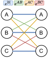
Figure 1: An illustration of our simulation: each edge corresponds to the variable that dictates the comparison based on the colour.

We consider both global and grouped-local explanations of the synthetic dataset in Figure 2 and Figure 3 respectively. In the global explanations, we explain all matches regardless of the cluster membership, while in the grouped-local explanations we only explain matches between items from $A$ against items from $B$. For more grouped-local explanations on different cluster pairs, we refer to appendix B.

Interpreting the simulation explanations.  The beehive plots showcase the recovered Pref-SHAP values, where the bar plots demonstrated the average Pref-SHAP values for each feature. The colour in the beehive plots indicates the magnitude of the difference between the corresponding features of the winner and of the loser in that match. For example, a red point in a beehive plot for feature $d$ indicates that the difference $x_{winner}^{(d)}-x_{loser}^{(d)}$ is large.

Fig. 2 illustrates the explanation results for the global synthetic experiments. We see that Pref-SHAP identified the within-cluster variable $x^{[0]}$ as the most important, which is a consequence of the fact that the largest number of matches are played between the items of the same cluster (cf. Fig. 1 where there are three blue lines and two lines of each of the other colours). The three inter-cluster variables contributed similarly according to Pref-SHAP, which, by symmetry, should be the case. Furthermore, the correct battle mechanism is captured by Pref-SHAP but not UPM, as we see that the large Pref-SHAP values for each feature are red in the beehive plot. This indicates that items with larger value are more likely to win against items with lower value in the corresponding features. In contrast, SHAP for UPM does not recover this insight.

The explanations for the matches between items from $A$ against items from $B$, are shown in Fig 3. Here, $x^{AB}$ is correctly picked as the relevant feature in these matches with Pref-SHAP, but not with SHAP for UPM. We see again that there is a clear tendency that large Pref-SHAP values are red for feature $x^{AB}$, showing that Pref-SHAP once again captures the designed gaming mechanism – which is not the case in SHAP for UPM. Intuitively, even though SHAP for UPM allows local explanations, it does so based on a global utility, which fails completely in a non-rankable case.

Pref-SHAP

SHAP for UPM

Pref-SHAP

SHAP for UPM

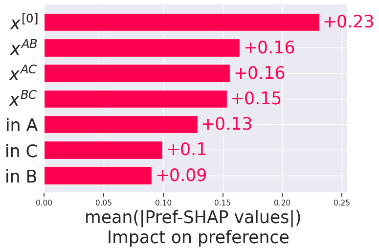
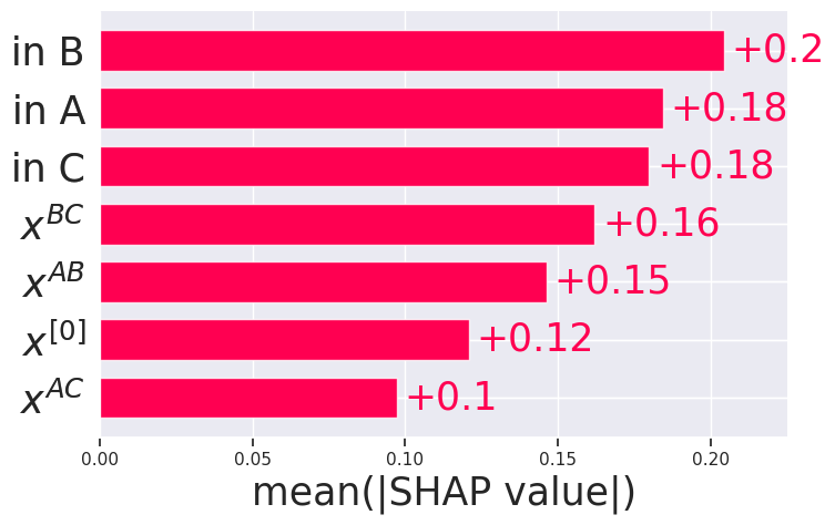
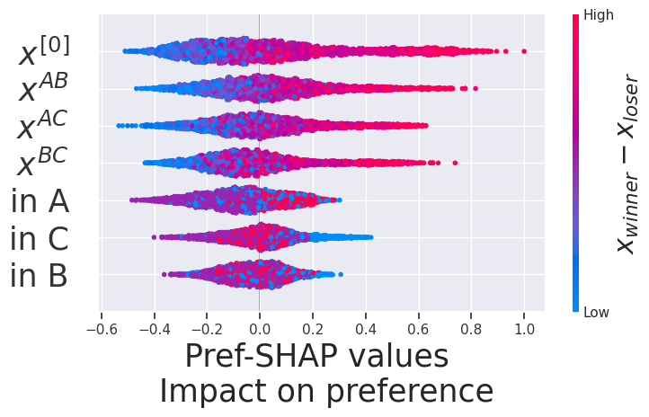
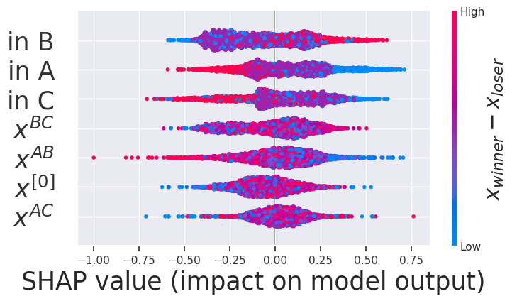
Figure 2: Bar and Beehive plots for global explanations on the synthetic dataset.

Pref-SHAP

SHAP for UPM

Pref-SHAP

SHAP for UPM

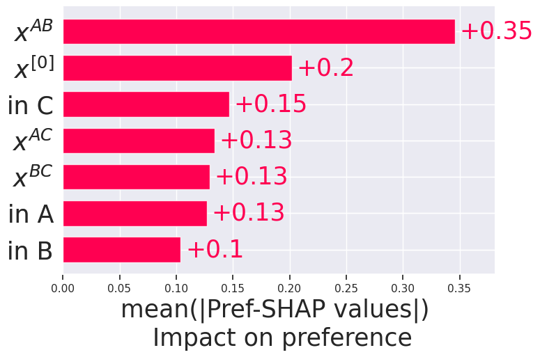
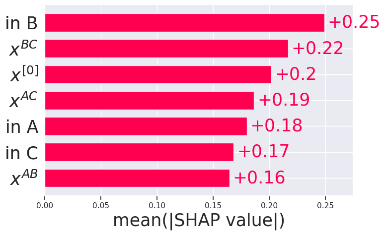
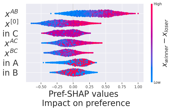
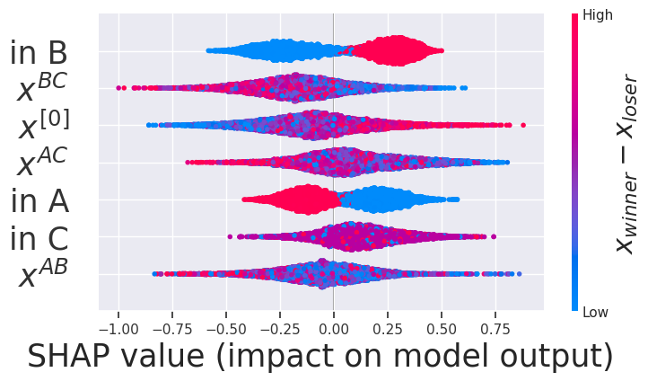
Figure 3: Bar and Beehive plots for grouped local explanations on the synthetic dataset (Cluster $A$ vs $B$).

Real-world explanations  For our real-world datasets, we consider publicly available datasets Chameleon, Pokémon and Tennis. We provide descriptive statistics of these datasets in Table 5 and give their brief descriptions below. Appendix B contains further large scale experiments on an additional dataset consisting of user-item interactions on a fashion retail website.

Table 2: Dataset summary

Dataset	$N_{\text{Matches}}$	$N_{\text{items}}$	$N_{\text{Context}}$	$D_{\text{continuous}}$	$D_{\text{binary}}$	$D^{\text{Context}}_{\text{continuous}}$	$D^{\text{Context}}_{\text{binary}}$
Synthetic	$40000$	$1000$	-	$4$	$3$	-	-
Chameleon	$106$	$35$	-	$7$	$19$	-	-
Pokémon	$60000$	$800$	-	$7$	$0$	-	-
Tennis	$95359$	$3483$	$4114$ (tournaments)	$4$	$7$	$0$	$6$

The Chameleon dataset [44] considers 106 contests between 35 male dwarf chameleons. Physical traits of the chameleons are measured such as the height of their casque, length of their jaw, body mass etc. According to [44], they fitted a linear Bradley Terry model and examined the coefficients to deduce that casque height (ch.res) and relative area of the flank patch (prop.patch) positively affected the fighting ability the most. The Pokémon dataset considers 60000 Pokémon battles among 800 Pokémon. Pokémon have different characteristics such as attack power, speed, health etc. The Pokémon further has at least one different type such as Electric, Water, Fire, etc. Certain types have advantages and disadvantages against each other, for instance, fire Pokémon are weak to water-based attacks (receiving twice the damage) and as a result have a disadvantage against water Pokémon.

The Tennis dataset considers professional tennis matches between 1991 and 2017 in all major tournaments each year. The data is provided publicly by ATP World Tour [45]. Features such as birthyear, weight, height etc are included about each tennis player together with context details of the match such as the court being indoor or outdoor and what surface the match is being played on.

The above datasets are not rankable, and we validate this claim by comparing GPM performance against UPM in Table 4, together with the estimated rankability measure SpecR proposed in [23] for each dataset. SpecR measures the similarity of the data to a complete dominance graph (i.e. rankable data). It takes values between 0 and 1 with values close to 1 being evidence in support of rankability. For the Tennis data where there are additional relationships with the context (tournaments), we estimate the average SpecR of each tournament.

Table 3: GPM vs UPM. Mean and standard deviations of performance averaged over 5 runs.

	Synthetic		Chameleon		Pokémon		Tennis
	GPM	UPM	GPM	UPM	GPM	UPM	C-GPM	UPM
Test AUC	$0.98_{\pm 0.00}$	$0.71_{\pm}0.01$	$0.92_{\pm 0.07}$	$0.80_{\pm 0.07}$	$0.86_{\pm 0.00}$	$0.82_{\pm 0.00}$	$0.58_{\pm 0.02}$	$0.52_{\pm 0.02}$
SpecR	$0.09$		$0.24$		$0.20$		$0.13_{\pm 0.07}$

Both the superior performance of GPM over UPM and the low SpecR measures suggest that the datasets are generally not rankable, which points to limitations of explaining preferences via utility-based modeling.

Explaining Pokémon battles.  We first consider standard dueling data for explaining preferences. We explain the learned preferences and learned differences in utilities on the Pokémon dataset in Figure 4. In this dataset, we have summed the Shapley values for Type features.

Pref-SHAP

SHAP for UPM

Pref-SHAP

SHAP for UPM

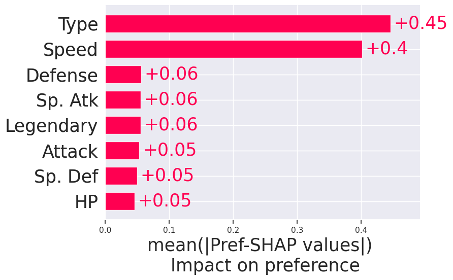
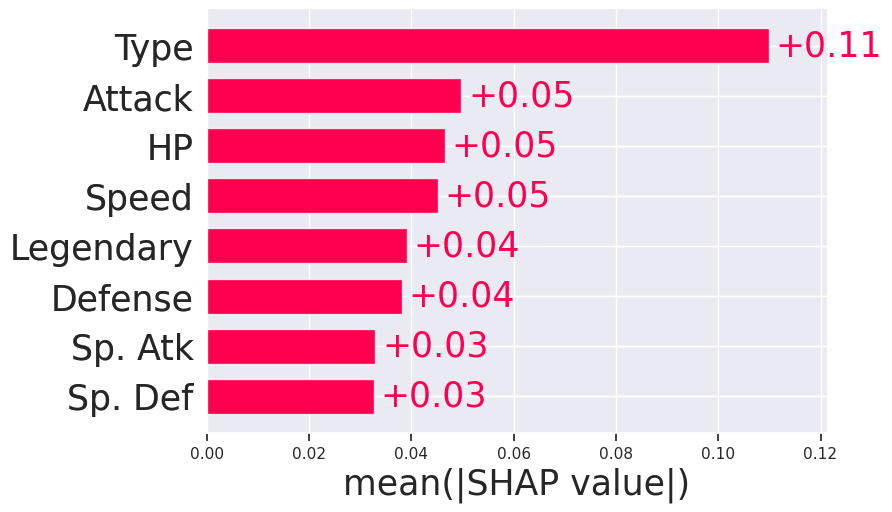
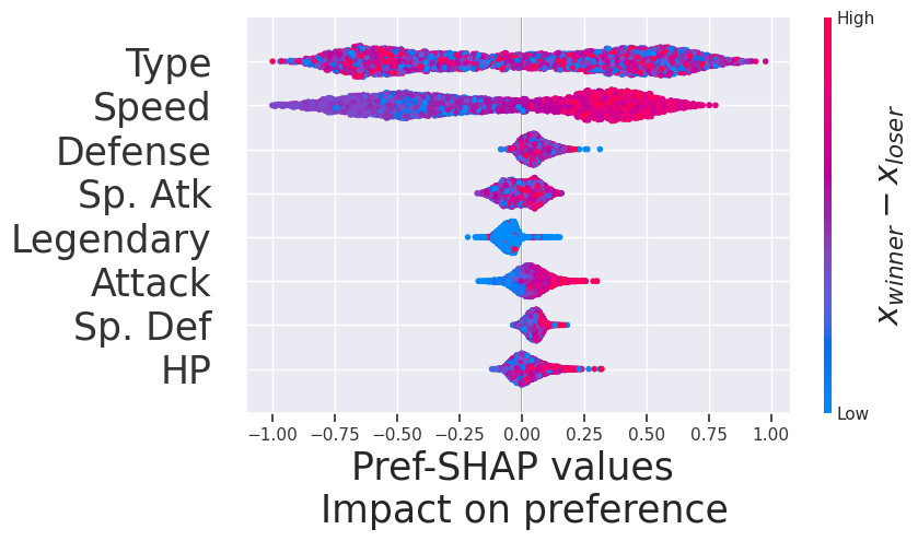
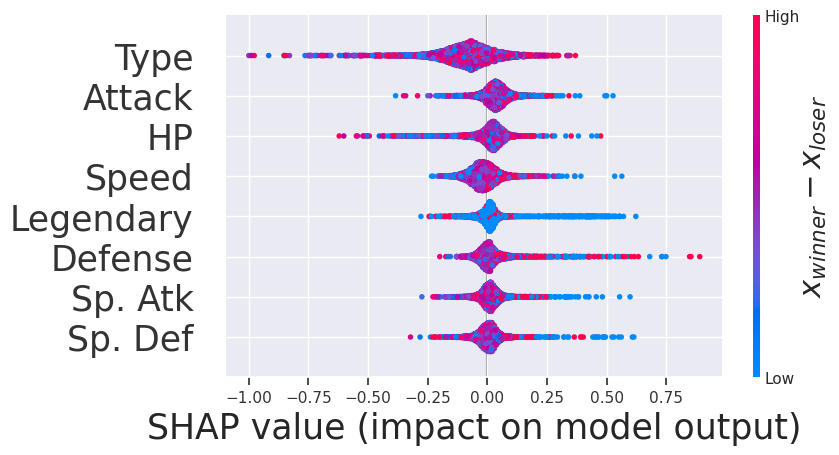
Figure 4: Bar and Beehive plots for the Pokémon dataset. Pref-SHAP captures that both speed and type matter, while SHAP for UPM only captures the type importance.

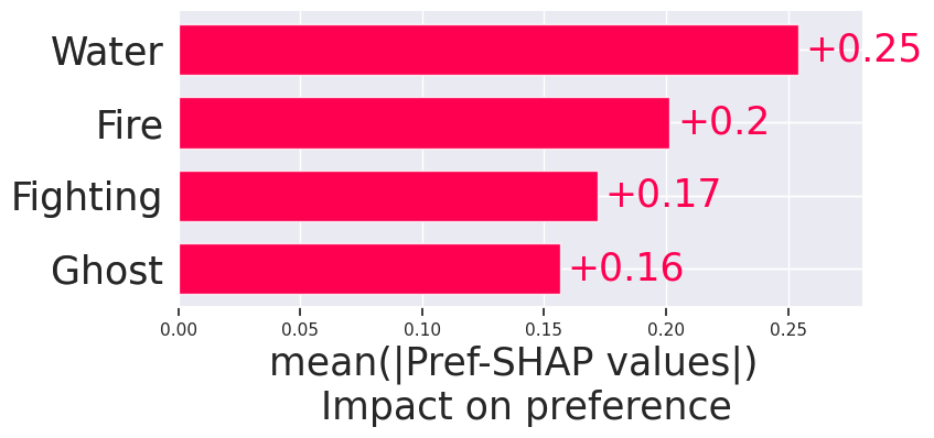
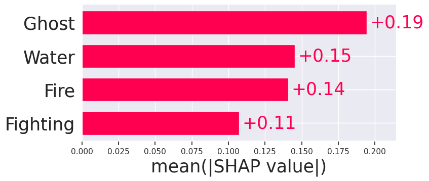
Figure 5: Explaining matches between 4 types of Pokémon, among them only fire and water has a type disadvantage/advantage against each other. Pref-SHAP (top) correctly identifies that fire and water are the most important, while water and fire are not deemed most important by SHAP for UPM.

We see that explaining general preferences provides further insight than just explaining the difference in utility functions. In particular, SHAP for UPM does not capture the additional importance of Speed in winning battles. As higher (more red) values of differences in speed $x^{\text{speed}}_{\text{winner}}-x^{\text{speed}}_{\text{loser}}$ have positive impact on the outcome, we conclude that having higher speed than your opponent is advantageous besides a type advantage. This insight is aligned with the “Sweeper” strategy [46], where one would employ a leading Pokémon with very high speed and attack to attempt downing the opponent before they can strike back. In Fig. 5, we see Pref-SHAP can also capture the correct type advantage/disadvantages among the Pokémon, but not SHAP for UPM.

Explaining Chameleon contests.  We find that UPM’s explanations are more aligned with [44]’s findings (prop.path and ch.res are the most important features), which is unsurprising since the Bradley Terry model used in [44] is also a utility based model. However, since GPM gives a much better predictive performance than UPM (Test AUC $0.92$ v.s. $0.80$), we believe Pref-SHAP’s explanations are also insightful. In fact, Pref-SHAP discovers that having larger jaw sizes (jl.res) than your opponent have a significant negative effect on match outcome, a previously undiscovered mechanism from [44]. We verify this finding in Appendix B by applying Pref-SHAP to GPM trained on multiple folds of the Chameleon dataset and consistently find that high values of the jaw size (jl.res) variable have a negative impact on the outcome.

Pref-SHAP

SHAP for UPM

Pref-SHAP

SHAP for UPM

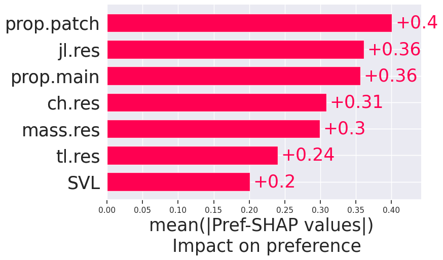
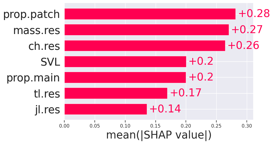
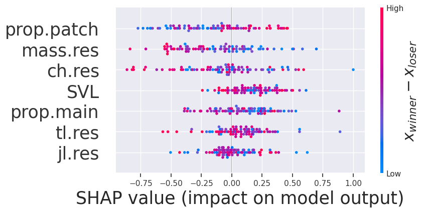
Figure 6: Bar and Beehive plots for the Chameleon dataset

Explaining Tennis matches.  We now consider preference learning with context covariates and explain both item characteristics and context covariates in Figure 7. In terms of item-based inference, Pref-SHAP finds that being older than your opponent ($x_{\text{winner}}^{\text{yob}}-x_{\text{loser}}^{\text{yob}}<0\to\text{Blue}$), physically heavier, and taller than your opponent positively impacts the chances of winning. We also find that debuting earlier as a professional tennis player than your opponent positively impacts your chances of winning. This is not surprising as debuting earlier may be indicative of a promising young talent. Across all competitions, there appear to be no significant patterns in environment effects.

Tennis players

Environment

Tennis players

Environment

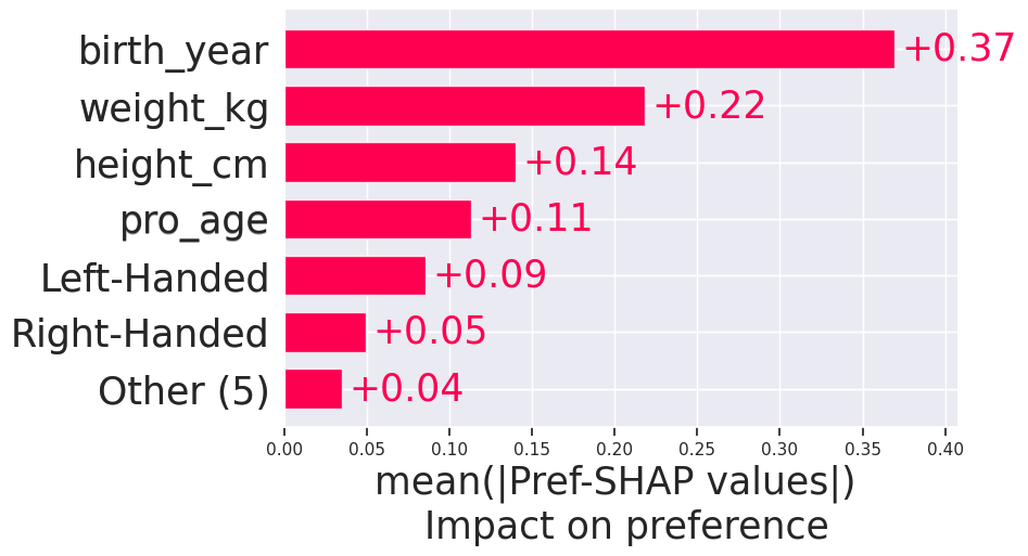
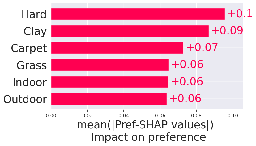
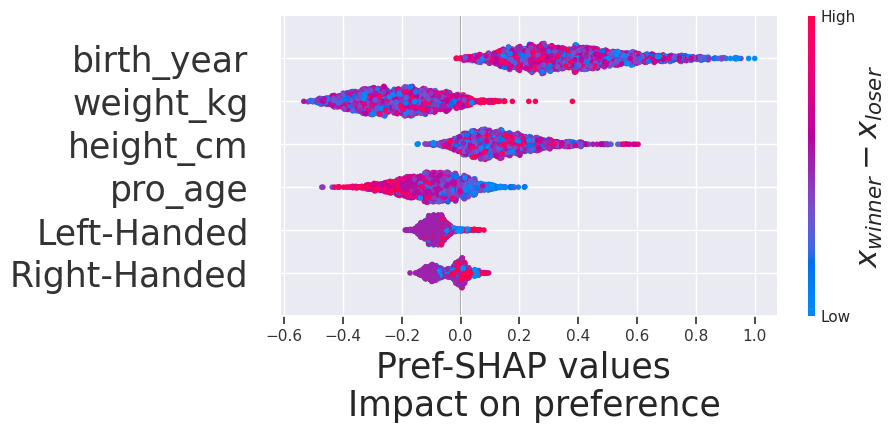
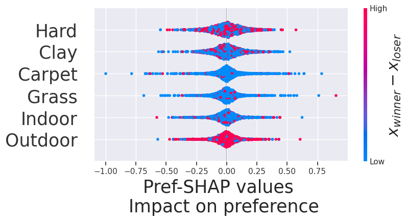
Figure 7: Item and context-specific Pref-SHAP values for the Tennis dataset
 

Explaining Djokovic’s losses  In plot Figure 8, we locally explain all Novak Djokovic’s losses in his professional career. Novak Djokovic is regarded as one of the greatest tennis players of all time, so understanding his weakness could serve as a practical demonstration of the utility of Pref-SHAP.

Djokovic

Environment

Djokovic

Environment

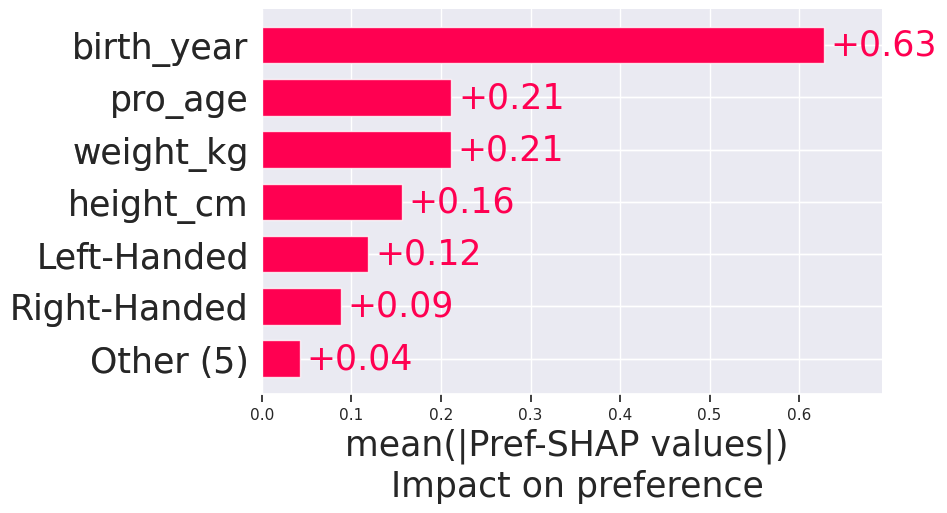
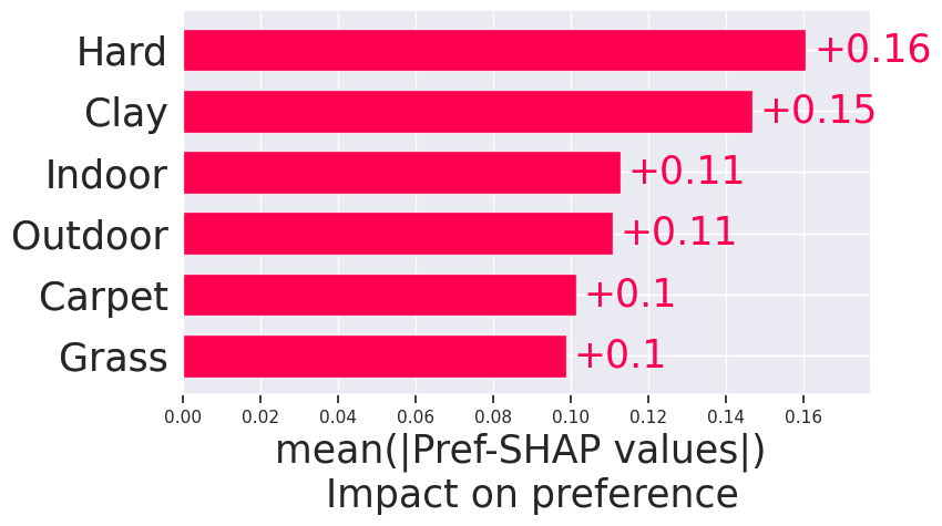
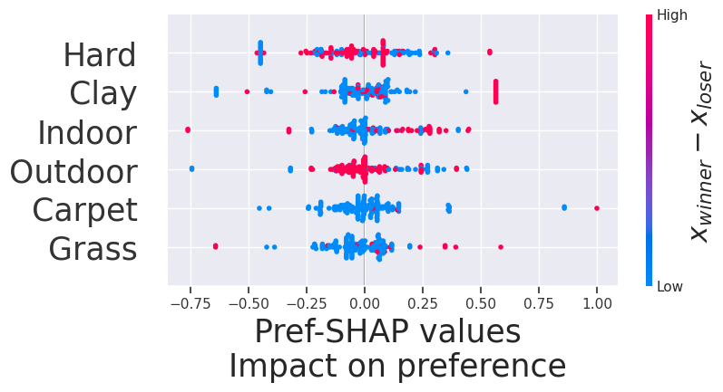
Figure 8: Local explanations of Djokovic losses
 

While the results take a similar shape to the global explanations, Djokovic remarkably seems to be weaker to players shorter than him, contrary to the general advantage of being taller. Besides this, Djokovic seems to be weaker on clay courts and when playing indoors.

5 Conclusion

In this work, we proposed Pref-SHAP to explain preference learning for pairwise comparison data. We proposed the appropriate value function for preference explanations and demonstrated the pathologies of the naive concatenation approach in Appendix B. Experiments demonstrated that Pref-SHAP recovers richer explanations than utility-based approaches, showcasing the ability of Pref-SHAP in interpreting the mechanism of preference elicitation.

Checklist

1. For all authors…

   1. Do the main claims made in the abstract and introduction accurately reflect the paper’s contributions and scope? [Yes]

   2. Did you describe the limitations of your work? [Yes]

   3. Did you discuss any potential negative societal impacts of your work? [N/A]

   4. Have you read the ethics review guidelines and ensured that your paper conforms to them? [Yes]

2. If you are including theoretical results…

   1. Did you state the full set of assumptions of all theoretical results? [Yes]

   2. Did you include complete proofs of all theoretical results? [Yes]

3. If you ran experiments…

   1. Did you include the code, data, and instructions needed to reproduce the main experimental results (either in the supplemental material or as a URL)? [Yes]

   2. Did you specify all the training details (e.g., data splits, hyperparameters, how they were chosen)? [Yes]

   3. Did you report error bars (e.g., with respect to the random seed after running experiments multiple times)? [N/A]

   4. Did you include the total amount of compute and the type of resources used (e.g., type of GPUs, internal cluster, or cloud provider)? See Appendix A [Yes]

4. If you are using existing assets (e.g., code, data, models) or curating/releasing new assets…

   1. If your work uses existing assets, did you cite the creators? [Yes]

   2. Did you mention the license of the assets? [N/A]

   3. Did you include any new assets either in the supplemental material or as a URL? [N/A]

   4. Did you discuss whether and how consent was obtained from people whose data you’re using/curating? [N/A]

   5. Did you discuss whether the data you are using/curating contains personally identifiable information or offensive content? [N/A]

5. If you used crowdsourcing or conducted research with human subjects…

   1. Did you include the full text of instructions given to participants and screenshots, if applicable? [N/A]

   2. Did you describe any potential participant risks, with links to Institutional Review Board (IRB) approvals, if applicable? [N/A]

   3. Did you include the estimated hourly wage paid to participants and the total amount spent on participant compensation? [N/A]

Appendix A Computation and Implementation Details

We propose several optimizations in the Pref-SHAP procedure. We consider fast sampling of coalitions $S$ in Algorithm 2 batched conjugate gradient descent in Algorithm 3 described below.
Fast coalitions  We first propose an optimized sampling scheme for finding coalitions $S$ in Algorithm 2.

Algorithm 2 Sampling unique $n$, $d$-dimensional coalitions in $\mathcal{O}(d)$ time

1:Number of coalitions $n$, number of features $d$.

2:$I=\text{SampleWithoutReplacement}(n,0,2^{d})$ $\triangleright$ Sample $n$ unique integers between $0$ and $2^{d}$

3:def base2(i): $\triangleright$ Convert integer to base-2 representation

4:     $S=[0,\ldots,0]\in\mathbb{R}^{d}$, $r=i$ $\triangleright$ Initialize $d$-dimensional 0 vector and the rest term $r$

5:     while $r>0$ do

6:         $i=\lfloor\log_{2}{(r)}\rfloor$ $\triangleright$ Find which index of $S$ to set to 1

7:         $S[i]=1$ $\triangleright$ Update $S$

8:         $r=r-2^{i}$ $\triangleright$ Update rest term

9:     end while

10:     return $S$ return $\{S_{1},\ldots S_{n}\}=\text{parallel\_apply}(I,\text{base2})$ $\triangleright$ Each integer can be independently converted

In contrast to the implementation in [14] which samples the weights from $p(Z)$, our method is embarrassingly parallel, which allows for an additional $\mathcal{O}(n)$ reduction. A naive algorithm that compares each sample $S_{i}$ has complexity $\mathcal{O}(n^{2}d^{2})$ and cannot be parallelized.
Stabilizing the Shapley value estimation We remove the features which have $0$ variance in the data we are explaining, similar to the implementation in SHAP. To ensure we get numerically stable Shapley Values, we calculate the inverse using Cholesky decomposition, as we found the regular inverse function provided inconsistent results.

To calculate CMEs effectively, we use preconditioned batched conjugate gradient descent over coalitions detailed in Algorithm 3.

Algorithm 3 Batched conjugate gradient descent

Preconditioner $P=\mathbf{K}_{\mathbf{x}_{D}}^{-1}$, batch $\mathbf{X}=[\mathbf{K}_{\mathbf{x}_{S_{i}}}\ldots\mathbf{K}_{\mathbf{x}_{S_{n}}}]$, $\mathbf{B}=[\mathbf{K}_{\mathbf{x}_{S_{i}},x_{S_{i}}}\ldots\mathbf{K}_{\mathbf{x}_{S_{n}},x_{S_{n}}}]$, max_its, tolerance $\varepsilon$

Set $\mathbf{R}=\mathbf{B}$, $\mathbf{Z}=\text{BatchMM}(P,\mathbf{B}),\mathbf{p}=\mathbf{Z}$, $\mathbf{a}=\mathbf{0}$

Set $\mathbf{R}_{Z}=[(\mathbf{R}_{i}\circ\mathbf{Z}_{i})_{++}\ldots(\mathbf{R}_{n}\circ\mathbf{Z}_{n})_{++}]$ $\triangleright$ Element wise product and sum

for  max_its do

     $\mathbf{L}=\text{BatchMM}(\mathbf{X},\mathbf{B})$

     $\boldsymbol{\alpha}=\mathbf{L}\circ\frac{1}{[(\mathbf{L}_{i}\circ\mathbf{p}_{i})_{++}\ldots(\mathbf{L}_{n}\circ\mathbf{p}_{n})_{++}]}$

     $\mathbf{a}=\mathbf{a}+\boldsymbol{\alpha}\circ\mathbf{p}$

     $\mathbf{r}=\mathbf{r}-\boldsymbol{\alpha}\circ\mathbf{L}$

     if Mean($[(\mathbf{r}_{i}\circ\mathbf{r}_{i})_{++}\ldots(\mathbf{r}_{n}\circ\mathbf{r}_{n})_{++}]$) < $\varepsilon$ then return $\mathbf{a}$

     end if

     $\mathbf{z}=\text{BatchMM}(P,\mathbf{r})$

     $\mathbf{R}_{Z}^{\text{new}}=[(\mathbf{R}_{i}\circ\mathbf{Z}_{i})_{++}\ldots(\mathbf{R}_{n}\circ\mathbf{Z}_{n})_{++}]$

     $\mathbf{p}=\mathbf{z}+[(\mathbf{R}_{i}^{\text{new}}\circ\frac{1}{\mathbf{R}_{i}})_{++}\ldots(\mathbf{R}_{n}^{\text{new}}\circ\frac{1}{\mathbf{R}_{n}})_{++}]\circ\mathbf{p}$

     $\mathbf{R}_{Z}=\mathbf{R}_{Z}^{\text{new}}$

end for

return $\mathbf{a}$

We have run all our jobs on one Nvidia V100 GPU.

Appendix B Additional Experimental Results

Naive Concatenation  We demonstrate the pathologies of the naive concatenation approach mentioned in Sec. 3 with our synthetic experiment. Recall that naive-concatenation approach here corresponds to first concatenating $\mathbf{x}^{(\ell)},\mathbf{x}^{(r)}$’s features together and applying SHAP to the learned function $g$ directly, in order to to obtain $2d$ Shapley values, instead of the original $d$, since each feature has been duplicated. This approach ignores that the items $\mathbf{x}^{(\ell)}$ and $\mathbf{x}^{(r)}$ in fact consist of the same features. Therefore, when we use the usual value function from SHAP (corresponding to the impact an individual feature has on the model when it is turned “off” by integration), we would be turning “off” the feature from the left item, while keeping “on” the feature from the right item, obtaining a difficult to interpret attribution score. This is highly problematic, as we might be inferring vastly different contributions of the same feature purely because of the item ordering when concatenating them. We note that the item ordering in all our experiments is arbitrary and carries no additional information about the match.

We can see from Fig. 9 that when we explain the preference model applied to the synthetic experiment, we see that, for example, $x^{AC}(l)$ from $\mathbf{x}^{(\ell)}$ and $x^{AC}(r)$ from $\mathbf{x}^{(r)}$ have in fact very different average Shapley values. Even attempting to average each pair of corresponding features does not give a meaningful feature contribution ordering ($x^{AB}$ and $x^{AC}$ are scored higher on average than $x^{BC}$ and $x^{[0]}$).

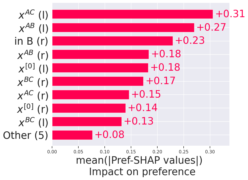
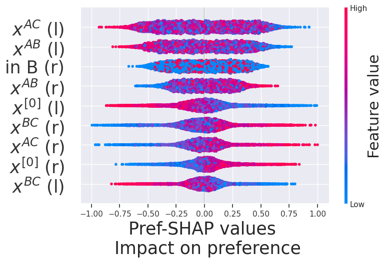
Figure 9: Explaining a naïve concatenation model

Additional synthetic data

We consider an additional synthetic experiment where we generate data directly from a GPM model and one where we construct synthetic dueling data. When simulating data, we first generate player covariates as ${\bf x}_{i}\in\mathbb{R}^{d}\sim\mathcal{N}(0,0.1\textbf{I}_{d})$ for each player $i$. When generating from the GPM model, we would set 2 covariates as important, by only keeping the 2 first entries of ${\bf x}_{i}$ and fixing the rest to be constant (equal to 0). We build a GPM model for $g$ out of these covariates and generate match outcomes.

We consider $d=10$, where only the two first features are set to be important in predicting the outcome.

Pref-SHAP

Explaining UPM

Pref-SHAP

Explaining UPM

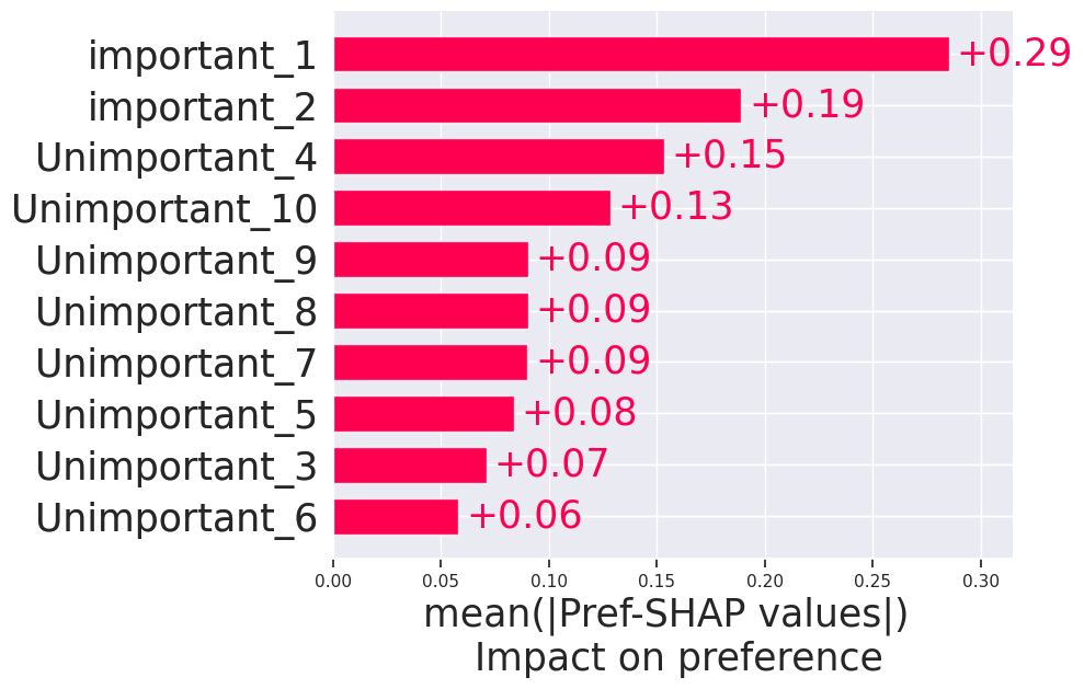
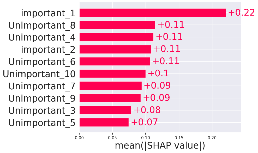
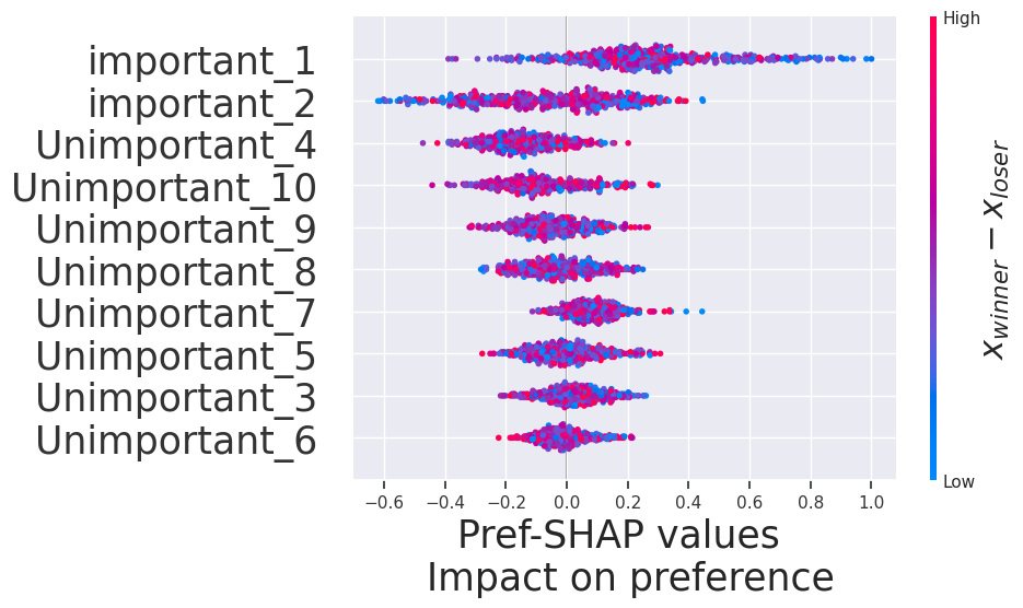
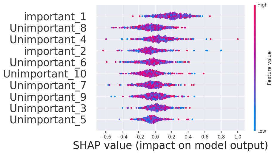
Figure 10: Bar and Beehive plots for Simulation A. Pref-SHAP recovers the correct features (1,2), while explaining UPM does not.

Chameleon data

We further provide explanations of the Chameleon dataset on several different folds in Figure 11 and Figure 12.

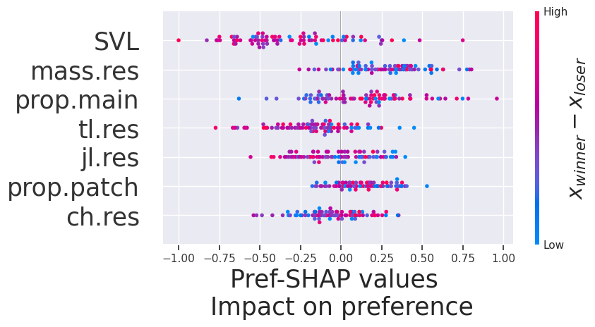
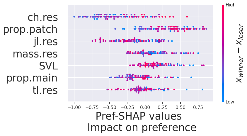
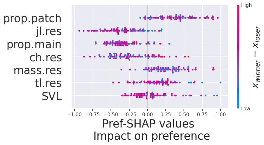
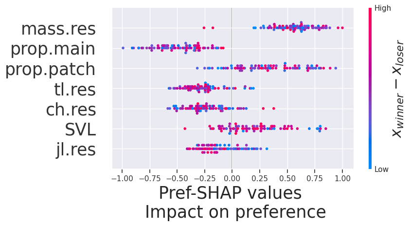
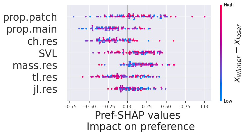
Figure 11: Pref-SHAP applied to 6 different folds of Chameleon. Pref-SHAP consistently finds that higher values of jaw length (jl.res) have a negative impact on outcome.

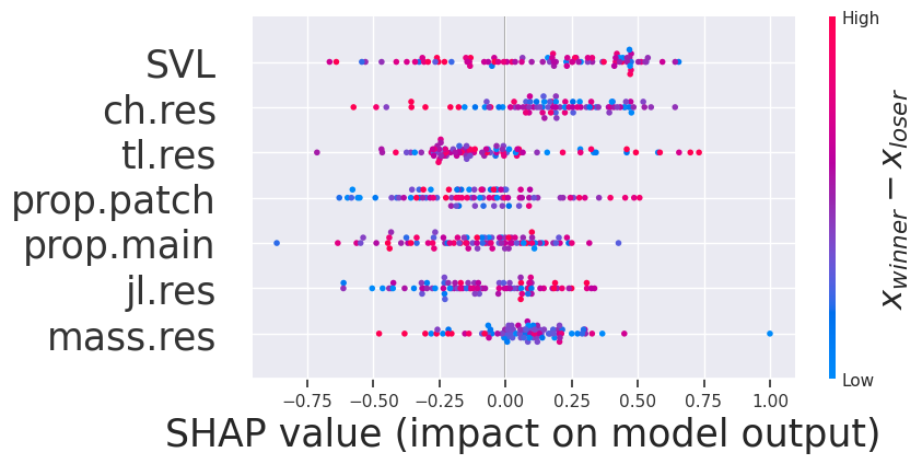
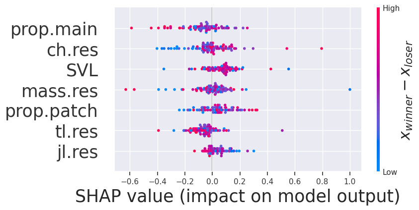
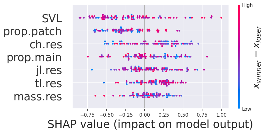
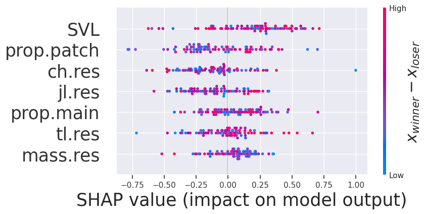
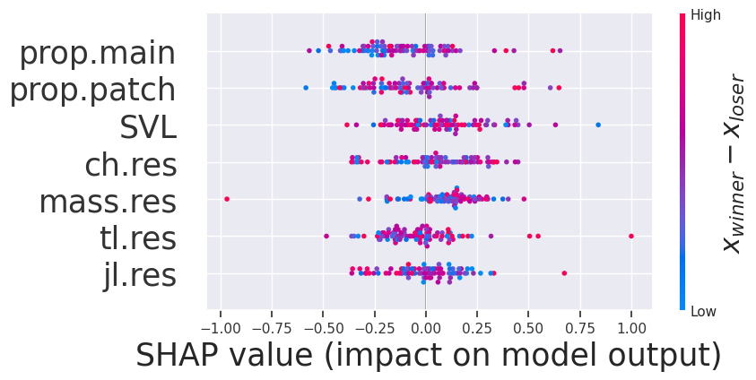
Figure 12: UPM explanations on 6 different folds of Chameleon. UPM is unable to find a consistent pattern for the impact of jaw length (jl.res) on the outcome.

Additional local explanations

We additionally provide local explanations on the synthetic dataset in Figure 13 and Figure 14.

Pref-SHAP

Explaining UPM

Pref-SHAP

Explaining UPM

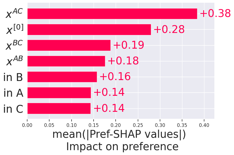
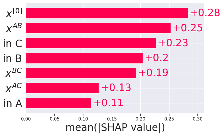
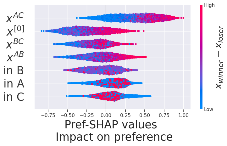
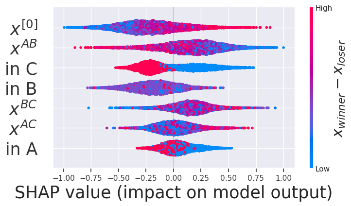
Figure 13: Explaining matches between clusters 0 and 2 on the synthetic dataset.

Pref-SHAP

Explaining UPM

Pref-SHAP

Explaining UPM

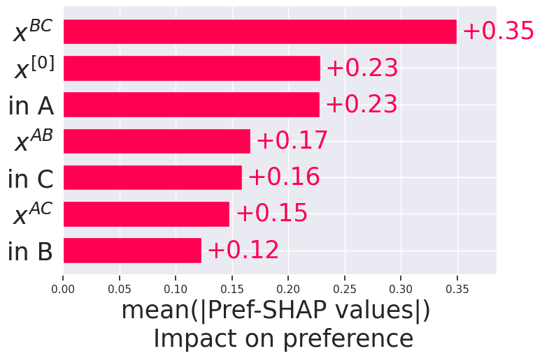
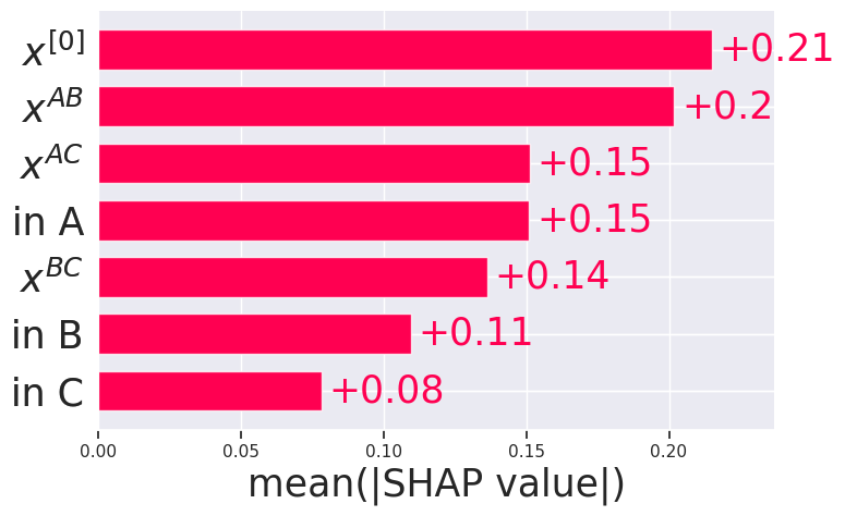
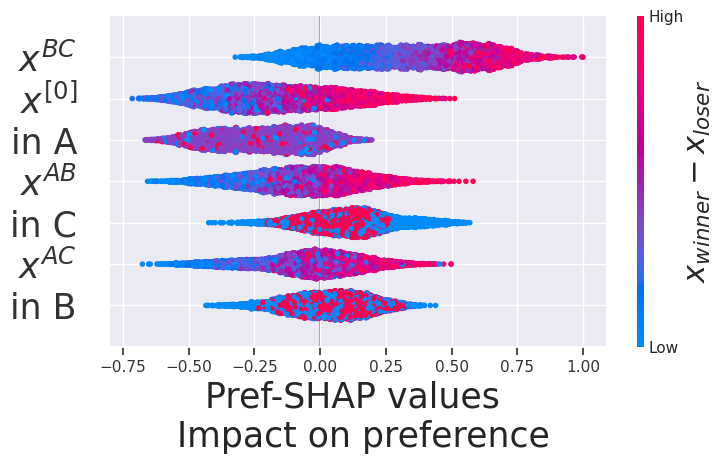
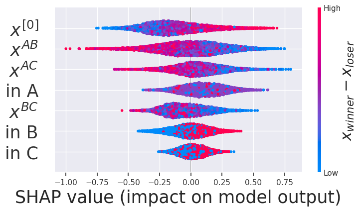
Figure 14: Explaining matches between clusters 1 and 2 on the synthetic dataset.

Website dataset

The Website dataset considers anonymized visitors on a fashion retail website, where we are given what garment each visitor viewed and what each visitor clicked in a session. A user may have more than one session. In this setup, we interpret a browsing session for a visitor as multiple matches between items, such that the winning item (clicked) competes against all losing items (only viewed). If several items are winners, they do not play against each other. Each item has several descriptive statistics such as colour, garment type, assortment characteristic etc. There are some limited descriptive statistics of the visitors, such as year of birth and gender code (i.e. Male/Female/Unspecified/Unknown).

Explaining Website  For the website dataset, we explain product and user preferences in Figure 15. We generally found that, for the period considered, cosmetic products and the “Jersey Basic category” drove clicks.

Products

User

Products

User

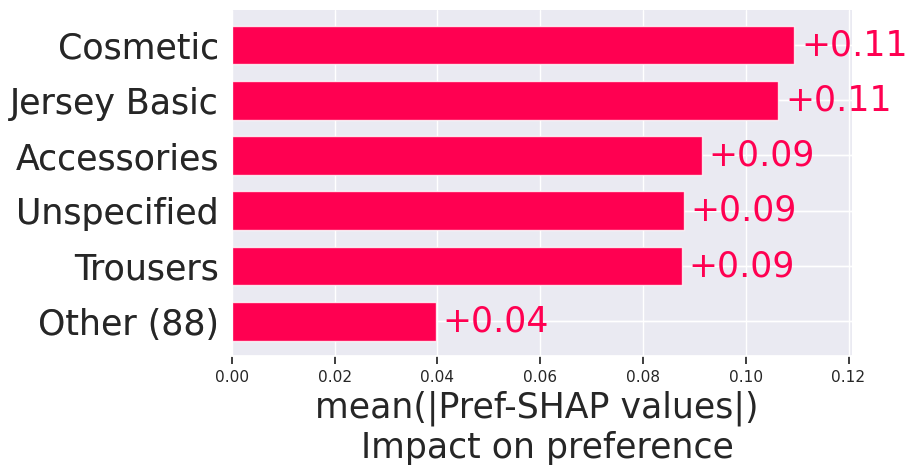
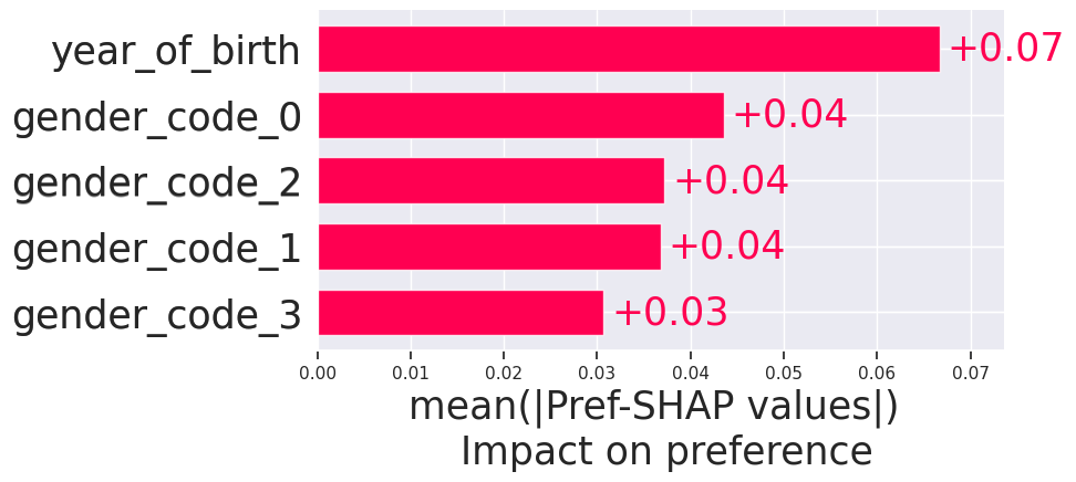
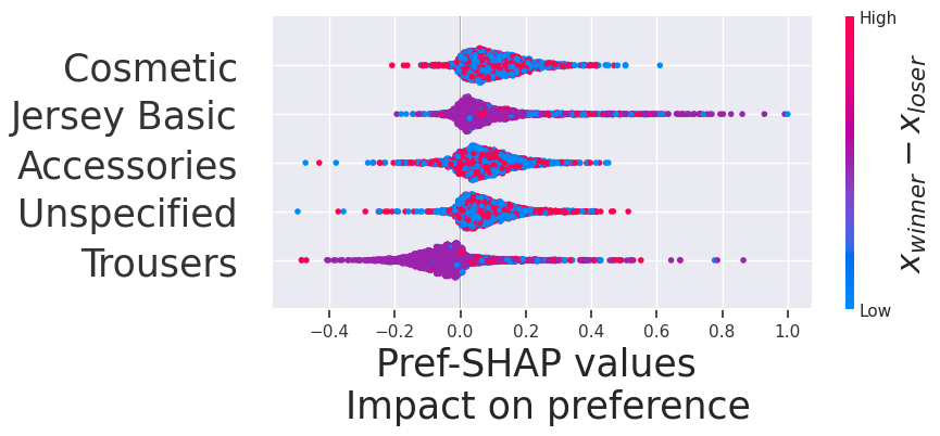
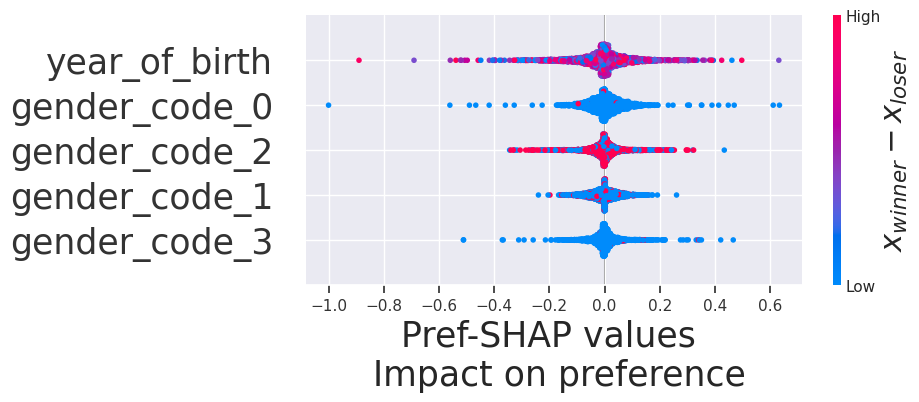
Figure 15: Barplots and beeplots for the website dataset, products on the left and user variables on the right.
 

Table 4: GPM vs UPM. Mean and standard deviations of performance averaged over 5 runs.

	Synthetic		Chameleon		Pokémon		Tennis		Website
	GPM	UPM	GPM	UPM	GPM	UPM	C-GPM	UPM	C-GPM	UPM
Test AUC	$0.98_{\pm 0.00}$	$0.71_{\pm 0.01}$	$0.92_{\pm 0.07}$	$0.80_{\pm 0.07}$	$0.86_{\pm 0.00}$	$0.82_{\pm 0.00}$	$0.58_{\pm 0.02}$	$0.52_{\pm 0.02}$	$0.66_{\pm 0.01}$	$0.65_{\pm 0.01}$
SpecR	$0.09$		$0.24$		$0.20$		$0.13_{\pm 0.07}$		$0.53_{\pm 0.10}$

Table 5: Dataset summary

Dataset	$N_{\text{Matches}}$	$N_{\text{Players}}$	$N_{\text{Context}}$	$D_{\text{continuous}}$	$D_{\text{binary}}$	$D^{\text{Context}}_{\text{continuous}}$	$D^{\text{Context}}_{\text{binary}}$
Website	$85144$	$20626$	$129117$ (users)	$0$	$93$	$1$	$4$

Appendix C Proofs

Proposition 3.1 (Preferential value functional for items).

Let $k$ be a product kernel on ${\mathcal{X}}$, i.e. $k(\mathbf{x}^{(\ell)},\mathbf{x}^{(r)})=\prod_{j=1}^{d}k^{(j)}(x^{(j)},x^{\prime(j)})$. Assume $k^{(j)}$ are bounded for all $j$, then the Riesz representation of the functional $\nu^{(p)}_{\mathbf{x}^{(\ell)},\mathbf{x}^{(r)},S}$ exists and takes the form:

$$\nu^{(p)}_{\mathbf{x}^{(\ell)},\mathbf{x}^{(r)},S}=\frac{1}{\sqrt{2}}\left({\mathcal{K}}(\mathbf{x}^{(\ell)},S)\otimes{\mathcal{K}}(\mathbf{x}^{(r)},S)-{\mathcal{K}}(\mathbf{x}^{(r)},S)\otimes{\mathcal{K}}(\mathbf{x}^{(\ell)},S)\right)$$

where ${\mathcal{K}}({\bf x},S)=k_{S}(\cdot,{\bf x}_{S})\otimes\mu_{X_{S^{c}}\mid X_{S}={\bf x}_{S}}$ and $k_{S}(\cdot,{\bf x}_{S})=\bigotimes_{j\in S}k^{(j)}(\cdot,x^{(j)})$ is the sub-product kernel defined analogously as $X_{S}$.

Proof.

From  [16], we know the generalised preferential kernel has the following feature map:

$$k_{E}((\mathbf{x}^{(\ell)},\mathbf{x}^{(r)}),\cdot)=\frac{1}{\sqrt{2}}\big{(}k(\cdot,\mathbf{x}^{(\ell)})\otimes k(\cdot,\mathbf{x}^{(r)})-k(\cdot,\mathbf{x}^{(r)})\otimes k(\cdot,\mathbf{x}^{(\ell)})\big{)}$$ (9)

where $\otimes$ are the usual tensor product. Recall we defined the preferential value function for items as,

$$\nu^{(p_{I})}_{\mathbf{x}^{(\ell)},\mathbf{x}^{(r)},S}(g)={\mathbb{E}}[g(X^{(\ell)},X^{(r)})\mid X_{S}^{(\ell)}=\mathbf{x}^{(\ell)}_{S},X_{S}^{(r)}=\mathbf{x}^{(r)}_{S}]$$ (10)

as $\nu^{(p_{I})}_{\mathbf{x}^{(\ell)},\mathbf{x}^{(r)},S}$ is a bounded linear functional on $g$ where $g\in{\mathcal{H}}_{k_{E}}$ is bounded, Riesz representation theorem [25] tells us there exists a Riesz representation of the functional in ${\mathcal{H}}_{k_{E}}$, which for notation simplicity, we will denote it as $\nu^{(p_{I})}_{\mathbf{x}^{(\ell)},\mathbf{x}^{(r)},S}$ as well. This corresponds to,

$$\nu^{(p_{I})}_{\mathbf{x}^{(\ell)},\mathbf{x}^{(r)},S}(g) ={\mathbb{E}}[g(X^{(\ell)},X^{(r)})\mid X_{S}^{(\ell)}=\mathbf{x}^{(\ell)}_{S},X_{S}^{(r)}=\mathbf{x}^{(r)}_{S}]$$ (11)

$$=\langle g,{\mathbb{E}}[k_{E}\left((X^{(\ell)},X^{(r)}),\cdot\right)\mid X_{S}^{(\ell)}=\mathbf{x}^{(\ell)}_{S},X_{S}^{(r)}=\mathbf{x}^{(r)}_{S}]\rangle_{{\mathcal{H}}_{k_{E}}}$$ (12)

$$=\langle g,\nu^{(p_{I})}_{\mathbf{x}^{(\ell)},\mathbf{x}^{(r)},S}\rangle_{{\mathcal{H}}_{k_{E}}}$$ (13)

now we expand the expectation of the feature map as,

$$\nu^{(p_{I})}_{\mathbf{x}^{(\ell)},\mathbf{x}^{(r)},S} ={\mathbb{E}}\left[\frac{1}{\sqrt{2}}\big{(}k(\cdot,X^{(\ell)})\otimes k(\cdot,X^{(r)})-k(\cdot,X^{(r)})\otimes k(\cdot,X^{(\ell)})\mid X_{S}^{(\ell)}=\mathbf{x}^{(\ell)}_{S},X_{S}^{(r)}=\mathbf{x}^{(r)}_{S}\right]$$ (14)

However, we note that

$${\mathbb{E}}[k(\cdot,X^{(\ell)})\otimes k(\cdot,X^{(r)})\mid X_{S}^{(\ell)}=\mathbf{x}^{(\ell)}_{S},X_{S}^{(r)}=\mathbf{x}^{(r)}_{S}] ={\mathbb{E}}[k(\cdot,X)\mid X_{S}=\mathbf{x}^{(\ell)}_{S}]$$

$$\quad\quad\quad\otimes{\mathbb{E}}[k(\cdot,X)\mid X_{S}=\mathbf{x}^{(r)}_{S}],$$

because $X^{(\ell)}$ and $X^{(r)}$ are identical copies of $X$ and we take the reference distribution as $p(X^{(\ell)},X^{(r)}\mid X_{S}^{(\ell)}=\mathbf{x}^{(\ell)}_{S},X_{S}^{(r)}=\mathbf{x}^{(r)}_{S})=p(X^{(\ell)}\mid X^{(\ell)}_{S}=\mathbf{x}^{(\ell)}_{S})p(X^{(r)}\mid X^{(r)}_{S}=\mathbf{x}^{(r)}_{S})$. Focusing on the duplicating component, we have,

$${\mathbb{E}}[k(\cdot,X)\mid X_{S}=\mathbf{x}^{(\ell)}] ={\mathbb{E}}[k_{S}(\cdot,X_{S})\otimes k_{S^{c}}(\cdot,X_{S^{c}})\mid X_{S}=\mathbf{x}^{(\ell)}_{S}]$$ (15)

$$=k_{S}(\cdot,\mathbf{x}^{(\ell)}_{S})\otimes{\mathbb{E}}[k_{S^{c}}(\cdot,X_{S^{c}})\mid X_{S}=\mathbf{x}^{(\ell)}_{S}]$$ (16)

$$=k_{S}(\cdot,\mathbf{x}^{(\ell)}_{S})\otimes\mu_{X_{S^{c}}\mid X_{S}=\mathbf{x}^{(\ell)}_{S}}$$ (17)

$$=:{\mathcal{K}}(\mathbf{x}^{(\ell)},S)$$ (18)

therefore by symmetry, we can arrange the terms in Eq 14 and conclude the proposition,

$$\nu^{(p_{I})}_{\mathbf{x}^{(\ell)},\mathbf{x}^{(r)},S}=\frac{1}{\sqrt{2}}\left({\mathcal{K}}(\mathbf{x}^{(\ell)},S)\otimes{\mathcal{K}}(\mathbf{x}^{(r)},S)-{\mathcal{K}}(\mathbf{x}^{(r)},S)\otimes{\mathcal{K}}(\mathbf{x}^{(\ell)},S)\right)$$ (19)

∎

To estimate the preferential value functional, we simply replace the conditional mean embeddings with the empirical versions, i.e. $\hat{{\mathcal{K}}}({\bf x},S)=k_{S}(\cdot,{\bf x}_{S})\otimes\hat{\mu}_{X_{{S^{c}}}\mid X_{S}={\bf x}_{S}}$, where $\hat{\mu}_{X_{{S^{c}}}\mid X_{S}={\bf x}_{S}}={\bf K}_{{\bf x}_{S},{\bf X}_{S}}({\bf K}_{{\bf X}_{S},{\bf X}_{S}}+n\lambda I)^{-1}{\bf\Phi}_{X_{{S^{c}}}}^{\top}$ is the standard conditional mean embedding estimator (${\bf\Phi}_{X_{{S^{c}}}}$ is the feature map matrix of rv $X_{{S^{c}}}$).

Now we proceed to estimate the preferential value function given a function $g$ from the RKHS,

Proposition 3.2 (Non-parametric Estimation).

Given $\hat{g}=\sum_{j=1}^{m}\alpha_{j}k_{E}((\mathbf{x}^{(\ell)}_{j},\mathbf{x}^{(r)}_{j}),\cdot)$, datasets $\mathbf{X}^{(\ell)},\mathbf{X}^{(r)}$, test items $\mathbf{x}^{(\ell)},\mathbf{x}^{(r)}$, the preferential value function at test items $\mathbf{x}^{(\ell)},\mathbf{x}^{(r)}$ for coalition $S$ and preference function $\hat{g}$ can be estimated as

$$\hat{\nu}_{\small\mathbf{x}^{(\ell)},\mathbf{x}^{(r)},S}^{(p_{I})}(\hat{g})=\boldsymbol{\alpha}^{\top}\left(\Gamma(\mathbf{X}^{(\ell)}_{S},\mathbf{x}^{(\ell)}_{S})\odot\Gamma(\mathbf{X}^{(r)}_{S},\mathbf{x}^{(r)}_{S})-\Gamma(\mathbf{X}^{(\ell)}_{S},\mathbf{x}^{(r)}_{S})\odot\Gamma(\mathbf{X}^{(r)}_{S},\mathbf{x}^{(\ell)}_{S})\right),$$

where $\Gamma(\mathbf{X}^{(\ell)}_{S},\mathbf{x}^{(\ell)}_{S})={\bf K}_{\mathbf{X}^{(\ell)}_{S},\mathbf{x}^{(\ell)}_{S}}\odot{\bf K}_{\mathbf{X}^{(\ell)}_{S^{c}},{\bf X}_{S^{c}}}{\bf K}_{{\bf X}_{S},\lambda}^{-1}{\bf K}_{{\bf X}_{S},\mathbf{x}^{(\ell)}_{S}},{\bf K}_{{\bf X}_{S},\lambda}={\bf K}_{{\bf X}_{S},{\bf X}_{S}}+n\lambda I$, $\boldsymbol{\alpha}=\{\alpha_{j}\}_{j=1}^{m}$ and $\lambda>0$ is a regularisation parameter.

Proof.

Given $\hat{g}$, the preferential value function evaluated at $\hat{g}$ can be written as,

$$\hat{\nu}_{\small\mathbf{x}^{(\ell)},\mathbf{x}^{(r)},S}^{(p_{I})}(\hat{g}) =\langle\hat{g},\hat{\nu}_{\small\mathbf{x}^{(\ell)},\mathbf{x}^{(r)},S}^{(p_{I})}\rangle_{{\mathcal{H}}_{k_{E}}}$$ (20)

$$=\langle\sum_{j=1}^{m}\alpha_{j}k_{E}((\mathbf{x}^{(\ell)}_{j},\mathbf{x}^{(r)}_{j}),\cdot),\frac{1}{\sqrt{2}}\left(\hat{{\mathcal{K}}}(\mathbf{x}^{(\ell)},S)\otimes\hat{{\mathcal{K}}}(\mathbf{x}^{(r)},S)-\hat{{\mathcal{K}}}(\mathbf{x}^{(r)},S)\otimes\hat{{\mathcal{K}}}(\mathbf{x}^{(\ell)},S)\right)\rangle_{{\mathcal{H}}_{k_{E}}}$$ (21)

$$=\frac{1}{\sqrt{2}}\left\langle\sum_{j=1}^{m}\alpha_{j}k_{E}((\mathbf{x}^{(\ell)}_{j},\mathbf{x}^{(r)}_{j}),\cdot),\hat{{\mathcal{K}}}(\mathbf{x}^{(\ell)},S)\otimes\hat{{\mathcal{K}}}(\mathbf{x}^{(r)},S)\right\rangle$$ (22)

$$\quad\quad\quad-\frac{1}{\sqrt{2}}\left\langle\sum_{j=1}^{m}\alpha_{j}k_{E}((\mathbf{x}^{(\ell)}_{j},\mathbf{x}^{(r)}_{j}),\cdot),\hat{{\mathcal{K}}}(\mathbf{x}^{(r)},S)\otimes\hat{{\mathcal{K}}}(\mathbf{x}^{(\ell)},S)\right\rangle$$ (23)

Now we focus on the first component, and rewrite:

$$\frac{1}{\sqrt{2}}\left\langle\sum_{j=1}^{m}\alpha_{j}k_{E}((\mathbf{x}^{(\ell)}_{j},\mathbf{x}^{(r)}_{j}),\cdot),\hat{{\mathcal{K}}}(\mathbf{x}^{(\ell)},S)\otimes\hat{{\mathcal{K}}}(\mathbf{x}^{(r)},S)\right\rangle=\sum_{j=1}^{m}A_{j}^{(1)}$$ (24)

and we continue to expand the terms,

$$A_{j}^{(1)} :=\frac{1}{\sqrt{2}}\left\langle\alpha_{j}k_{E}((\mathbf{x}^{(\ell)}_{j},\mathbf{x}^{(r)}_{j}),\cdot),\hat{{\mathcal{K}}}(\mathbf{x}^{(\ell)},S)\otimes\hat{{\mathcal{K}}}(\mathbf{x}^{(r)},S)\right\rangle$$ (25)

$$=\frac{1}{\sqrt{2}}\left\langle\frac{\alpha_{j}}{\sqrt{2}}\big{(}k(\cdot,\mathbf{x}^{(\ell)}_{j})\otimes k(\cdot,\mathbf{x}^{(r)}_{j})-k(\cdot,\mathbf{x}^{(r)}_{j})\otimes k(\cdot,\mathbf{x}^{(\ell)}_{j})\big{)},\hat{{\mathcal{K}}}(\mathbf{x}^{(\ell)},S)\otimes\hat{{\mathcal{K}}}(\mathbf{x}^{(r)},S)\right\rangle$$ (26)

$$=\frac{\alpha_{j}}{2}\left(\left\langle k(\cdot,\mathbf{x}^{(\ell)}_{j})\otimes k(\cdot,\mathbf{x}^{(r)}_{j}),\hat{{\mathcal{K}}}(\mathbf{x}^{(\ell)},S)\otimes\hat{{\mathcal{K}}}(\mathbf{x}^{(r)},S)\right\rangle-\left\langle k(\cdot,\mathbf{x}^{(r)}_{j})\otimes k(\cdot,\mathbf{x}^{(\ell)}_{j}),\hat{{\mathcal{K}}}(\mathbf{x}^{(\ell)},S)\otimes\hat{{\mathcal{K}}}(\mathbf{x}^{(r)},S)\right\rangle\right)$$ (27)

$$=\frac{\alpha_{j}}{2}\left(A_{j}^{(1,\ell)}-A_{j}^{(1,r)}\right)$$ (28)

We then note that

$$A_{j}^{(1,\ell)} :=\left\langle k(\cdot,\mathbf{x}^{(\ell)}_{j}))\otimes k(\cdot,\mathbf{x}^{(r)}_{j}),\hat{{\mathcal{K}}}(\mathbf{x}^{(\ell)},S)\otimes\hat{{\mathcal{K}}}(\mathbf{x}^{(r)},S)\right\rangle$$ (29)

$$=\left\langle k(\cdot,\mathbf{x}^{(\ell)}_{j}),\hat{{\mathcal{K}}}(\mathbf{x}^{(\ell)},S)\right\rangle\left\langle k(\cdot,\mathbf{x}^{(r)}_{j}),\hat{{\mathcal{K}}}(\mathbf{x}^{(r)},S)\right\rangle$$ (30)

$$=k_{S}(\mathbf{x}^{(\ell)}_{j},\mathbf{x}^{(\ell)}){\bf K}_{{\mathbf{x}^{(\ell)}_{j}}_{S},{\bf X}_{S}}({\bf K}_{{\bf X}_{S},{\bf X}_{S}}+n\lambda I)^{-1}{\bf K}_{{\bf X}_{{S^{c}}},\mathbf{x}^{(\ell)}_{{S^{c}}}}$$ (31)

$$\quad\quad\quad\times k_{S}(\mathbf{x}^{(r)}_{j},\mathbf{x}^{(r)}){\bf K}_{{\mathbf{x}^{(r)}_{j}}_{S},{\bf X}_{S}}({\bf K}_{{\bf X}_{S},{\bf X}_{S}}+n\lambda I)^{-1}{\bf K}_{{\bf X}_{{S^{c}}},\mathbf{x}^{(r)}_{{S^{c}}}}$$ (32)

$$=\Gamma(\mathbf{x}^{(\ell)}_{j_{S}},\mathbf{x}^{(\ell)}_{S})\odot\Gamma(\mathbf{x}^{(r)}_{j_{S}},\mathbf{x}^{(r)}_{S})$$ (33)

To go from the second equation to the third equation in this paragraph, realise $k(\cdot,\mathbf{x}^{(\ell)})=k_{S}(\cdot,\mathbf{x}^{(\ell)}_{S})\otimes k_{{S^{c}}}(\cdot,\mathbf{x}^{(\ell)}_{{S^{c}}})$ by product kernel assumption. In this case, we can rewrite $A_{j}^{(1)}$ as,

$$A_{j}^{(1)}=\frac{\alpha_{j}}{2}\left(\Gamma(\mathbf{x}^{(\ell)}_{j_{S}},\mathbf{x}^{(\ell)}_{S})\odot\Gamma(\mathbf{x}^{(r)}_{j_{S}},\mathbf{x}^{(r)}_{S})-\Gamma(\mathbf{x}^{(r)}_{j_{S}},\mathbf{x}^{(\ell)}_{S})\odot\Gamma(\mathbf{x}^{(\ell)}_{j_{S}},\mathbf{x}^{(r)}_{S})\right)$$ (34)

Analogously, define $\sum A_{j}^{(2)}$ as the second component after the subtraction sign, by symmetry, we know

$$A_{j}^{(2)}=\frac{\alpha_{j}}{2}\left(\Gamma(\mathbf{x}^{(\ell)}_{j_{S}},\mathbf{x}^{(r)}_{S})\odot\Gamma(\mathbf{x}^{(r)}_{j_{S}},\mathbf{x}^{(\ell)}_{S})-\Gamma(\mathbf{x}^{(r)}_{j_{S}},\mathbf{x}^{(r)}_{S})\odot\Gamma(\mathbf{x}^{(\ell)}_{j_{S}},\mathbf{x}^{(\ell)}_{S})\right)$$ (35)

by subtracting $A_{j}^{(1)}$ and $A_{j}^{(1)}$, we get the following:

$$\hat{\nu}_{\small\mathbf{x}^{(\ell)},\mathbf{x}^{(r)},S}^{(p_{I})}(\hat{g}) =\sum_{j=1}^{m}\alpha_{j}\left(\Gamma(\mathbf{x}^{(\ell)}_{j_{S}},\mathbf{x}^{(\ell)}_{S})\odot\Gamma(\mathbf{x}^{(r)}_{j_{S}},\mathbf{x}^{(r)}_{S})-\Gamma(\mathbf{x}^{(r)}_{j_{S}},\mathbf{x}^{(\ell)}_{S})\odot\Gamma(\mathbf{x}^{(\ell)}_{j_{S}},\mathbf{x}^{(r)}_{S})\right)$$ (36)

writing it in compact form, we arrive to our result,

$$=\boldsymbol{\alpha}^{\top}\left(\Gamma(\mathbf{X}^{(\ell)}_{S},\mathbf{x}^{(\ell)}_{S})\odot\Gamma(\mathbf{X}^{(r)}_{S},\mathbf{x}^{(r)}_{S})-\Gamma(\mathbf{X}^{(\ell)}_{S},\mathbf{x}^{(r)}_{S})\odot\Gamma(\mathbf{X}^{(r)}_{S},\mathbf{x}^{(\ell)}_{S})\right)$$ (37)

∎

Proposition 3.3 (Preferential value function for contexts).

Given a preference function $g_{U}\in{\mathcal{H}}_{k_{E}^{U}}$, denote $\Omega^{\prime}=\{1,...,d^{\prime}\}$, then the utility of context features $S^{\prime}\subseteq\Omega^{\prime}$ on $\{{\bf u},\mathbf{x}^{(\ell)},\mathbf{x}^{(r)}\}$ is measured by $\nu^{(p_{U})}_{{\bf u},\mathbf{x}^{(\ell)},\mathbf{x}^{(r)},S^{\prime}}(g_{U})={\mathbb{E}}[g_{U}\left(\{{\bf u}_{S^{\prime}},U_{{S^{\prime}}^{c}}\},\mathbf{x}^{(\ell)},\mathbf{x}^{(r)}\right)\mid U_{S^{\prime}}={\bf u}_{S^{\prime}}]$ where the expectation is taken over the observational distribution of $U$. Now, given a test triplet (${\bf u},\mathbf{x}^{(\ell)},\mathbf{x}^{(r)})$, if $\hat{g}_{U}=\sum_{j=1}^{m}\alpha_{j}k_{E}^{U}\left(({\bf u}_{j},\mathbf{x}^{(\ell)}_{j},\mathbf{x}^{(r)}_{j}),\cdot\right)$, the non-parametric estimator is:

$$\hat{\nu}^{(p_{U})}_{{\bf u},\mathbf{x}^{(\ell)},\mathbf{x}^{(r)},S^{\prime}}(\hat{g}_{U}) =\boldsymbol{\alpha}^{\top}\left(\left({\bf K}_{{\bf U}_{S^{\prime}},{\bf u}_{S^{\prime}}}\odot{\bf K}_{{\bf U}_{S^{\prime c}},{\bf U}_{S^{\prime c}}}\left({\bf K}_{{\bf U}_{S^{\prime}},{\bf U}_{S^{\prime}}}+m\lambda^{\prime}I\right)^{-1}{\bf K}_{{\bf U}_{S^{\prime}},{\bf u}_{S^{\prime}}}\right)\odot\Xi_{\mathbf{x}^{(\ell)},\mathbf{x}^{(r)}}\right)$$

where $\Xi_{\mathbf{x}^{(\ell)},\mathbf{x}^{(r)}}=\left({\bf K}_{\mathbf{X}^{(\ell)},\mathbf{x}^{(\ell)}}\odot{\bf K}_{\mathbf{X}^{(r)},\mathbf{x}^{(r)}}-{\bf K}_{\mathbf{X}^{(r)},\mathbf{x}^{(\ell)}}\odot{\bf K}_{\mathbf{X}^{(\ell)},\mathbf{x}^{(r)}}\right)$.

Proof.

Recall the feature map of the kernel $k_{E}^{U}$ takes the following form,

$$k_{E}^{U}\left(({\bf u},\mathbf{x}^{(\ell)},\mathbf{x}^{(r)}),\cdot\right)=k_{u}({\bf u},\cdot)\otimes k_{E}((\mathbf{x}^{(\ell)},\mathbf{x}^{(r)}),\cdot)$$ (38)

Therefore we can express the preferential value function for context as,

$$\nu^{(p_{U})}_{{\bf u},\mathbf{x}^{(\ell)},\mathbf{x}^{(r)},S^{\prime}}(g_{U}) ={\mathbb{E}}\left[g_{U}\left(\{{\bf u}_{S^{\prime}},U_{{S^{c}}}\},\mathbf{x}^{(\ell)},\mathbf{x}^{(r)}\right)\mid U_{S}={\bf u}_{S^{\prime}}\right]$$ (39)

$$=\left\langle g_{U},{\mathbb{E}}\left[k_{E}^{U}\left((\{{\bf u}_{S^{\prime}},U_{{S^{\prime}}^{c}}\},\mathbf{x}^{(\ell)},\mathbf{x}^{(r)}),\cdot\right)\mid U_{S^{\prime}}={\bf u}_{S^{\prime}}\right]\right\rangle$$ (40)

$$=\left\langle g_{U},{\mathbb{E}}\left[k_{u}(\{{\bf u}_{S^{\prime}},U_{S^{c}}\}\mid U_{S^{\prime}}={\bf u}_{S^{\prime}}\right]\otimes k_{E}((\mathbf{x}^{(\ell)},\mathbf{x}^{(r)}),\cdot)\right\rangle$$ (41)

$$=\left\langle g_{U},k_{u_{S^{\prime}}}({\bf u}_{S^{\prime}})\otimes\mu_{U_{{S^{\prime}}^{c}}\mid U_{S^{\prime}}={\bf u}_{S^{\prime}}}\otimes k_{E}((\mathbf{x}^{(\ell)},\mathbf{x}^{(r)}),\cdot)\right\rangle$$ (42)

The remaining steps are analogous to [12, Prop.2]. To obtain the empirical estimation, we first replace the conditional mean embedding $\mu_{U_{{S^{\prime}}^{c}}\mid U_{S^{\prime}}={\bf u}_{S^{\prime}}}$ with its empirical estimate and replace $g_{U}$ with $\hat{g}_{U}=\sum_{j=1}^{m}\alpha_{j}k_{E}^{U}\left(({\bf u}_{j},\mathbf{x}^{(\ell)}_{j},\mathbf{x}^{(r)}_{j}),\cdot\right)$. Now the empirical estimator has the following form,

$$\small\hat{\nu}^{(p_{U})}_{{\bf u},\mathbf{x}^{(\ell)},\mathbf{x}^{(r)},S^{\prime}}(\hat{g}_{U}) =\left\langle\sum_{j=1}^{m}\alpha_{j}k_{E}^{U}\left(({\bf u}_{j},\mathbf{x}^{(\ell)}_{j},\mathbf{x}^{(r)}_{j}),\cdot\right),k_{u_{S^{\prime}}}({\bf u}_{S^{\prime}})\otimes\hat{\mu}_{U_{{S^{\prime}}^{c}}\mid U_{S^{\prime}}={\bf u}_{S^{\prime}}}\otimes k_{E}((\mathbf{x}^{(\ell)},\mathbf{x}^{(r)}),\cdot)\right\rangle$$ (43)

$$=\sum_{j=1}^{m}\alpha_{j}\left\langle k_{u}({\bf u}_{j},\cdot)\otimes k_{E}((\mathbf{x}^{(\ell)}_{j},\mathbf{x}^{(r)}_{j}),\cdot),k_{u_{S^{\prime}}}({\bf u}_{S^{\prime}})\otimes\hat{\mu}_{U_{{S^{\prime}}^{c}}\mid U_{S^{\prime}}={\bf u}_{S^{\prime}}}\otimes k_{E}((\mathbf{x}^{(\ell)},\mathbf{x}^{(r)}),\cdot)\right\rangle$$ (44)

$$=\sum_{j=1}^{m}\alpha_{j}\left\langle k_{u}({\bf u}_{j},\cdot),k_{u_{S}}({\bf u}_{S})\otimes\hat{\mu}_{U_{{S^{\prime}}^{c}}\mid U_{S}={\bf u}_{S}}\right\rangle k_{E}\left((\mathbf{x}^{(\ell)}_{j},\mathbf{x}^{(r)}_{j}),(\mathbf{x}^{(\ell)},\mathbf{x}^{(r)})\right)$$ (45)

Now write everything in terms of matrices,

$$=\boldsymbol{\alpha}^{\top}\left(\left({\bf K}_{{\bf U}_{S^{\prime}},{\bf u}_{S^{\prime}}}\odot{\bf K}_{{\bf U}_{S^{\prime c}},{\bf U}_{S^{\prime c}}}\left({\bf K}_{{\bf U}_{S^{\prime}},{\bf U}_{S^{\prime}}}+m\lambda^{\prime}I\right)^{-1}{\bf K}_{{\bf U}_{S^{\prime}},{\bf u}_{S^{\prime}}}\right)\odot\Xi_{\mathbf{x}^{(\ell)},\mathbf{x}^{(r)}}\right)$$ (46)

where $\Xi_{\mathbf{x}^{(\ell)},\mathbf{x}^{(r)}}=\left({\bf K}_{\mathbf{X}^{(\ell)},\mathbf{x}^{(\ell)}}\odot{\bf K}_{\mathbf{X}^{(r)},\mathbf{x}^{(r)}}-{\bf K}_{\mathbf{X}^{(r)},\mathbf{x}^{(\ell)}}\odot{\bf K}_{\mathbf{X}^{(\ell)},\mathbf{x}^{(r)}}\right)$. ∎

References

- Fürnkranz and Hüllermeier [2003] Johannes Fürnkranz and Eyke Hüllermeier. Pairwise preference learning and ranking. In Nada Lavrač, Dragan Gamberger, Hendrik Blockeel, and Ljupčo Todorovski, editors, Machine Learning: ECML 2003, pages 145–156, Berlin, Heidelberg, 2003. Springer Berlin Heidelberg. ISBN 978-3-540-39857-8.
- Bradley and Terry [1952] Ralph Allan Bradley and Milton E. Terry. Rank analysis of incomplete block designs: I. The method of paired comparisons. Biometrika, 39(3/4):324–345, 1952.
- Thurstone [1994] Louis L Thurstone. A law of comparative judgment. Psychological review, 101(2):266, 1994.
- Chu and Ghahramani [2005] Wei Chu and Zoubin Ghahramani. Preference learning with Gaussian processes. In Proceedings of the 22nd International Conference on Machine Learning, pages 137–144, 2005.
- González et al. [2017] Javier González, Zhenwen Dai, Andreas Damianou, and Neil D Lawrence. Preferential Bayesian optimization. In Proceedings of the 34th International Conference on Machine Learning, pages 1282–1291, 2017.
- Cattelan et al. [2013] Manuela Cattelan, Cristiano Varin, and David Firth. Dynamic bradley–terry modelling of sports tournaments. Journal of the Royal Statistical Society: Series C (Applied Statistics), 62(1):135–150, 2013.
- Chau et al. [2020] Siu Lun Chau, Mihai Cucuringu, and Dino Sejdinovic. Spectral ranking with covariates. arXiv preprint arXiv:2005.04035, 2020.
- Kahneman and Tversky [1979] Daniel Kahneman and Amos Tversky. On the interpretation of intuitive probability: A reply to Jonathan Cohen. Cognition, 7(4):409–411, 1979.
- Houlsby et al. [2012] Neil Houlsby, Ferenc Huszar, Zoubin Ghahramani, and Jose M Hernández-Lobato. Collaborative gaussian processes for preference learning. In Advances in neural information processing systems, pages 2096–2104, 2012.
- Bennett et al. [2022] Stefanos Bennett, Mihai Cucuringu, and Gesine Reinert. Lead-lag detection and network clustering for multivariate time series with an application to the us equity market. arXiv preprint arXiv:2201.08283, 2022.
- Stuart-Fox et al. [2006a] Devi M Stuart-Fox, David Firth, Adnan Moussalli, and Martin J Whiting. Multiple signals in chameleon contests: designing and analysing animal contests as a tournament. Animal Behaviour, 71(6):1263–1271, 2006a.
- Chau et al. [2021] Siu Lun Chau, Javier Gonzalez, and Dino Sejdinovic. RKHS-SHAP: Shapley values for kernel methods. arXiv preprint arXiv:2110.09167, 2021.
- Ribeiro et al. [2016] Marco Tulio Ribeiro, Sameer Singh, and Carlos Guestrin. "why should I trust you?": Explaining the predictions of any classifier. In Proceedings of the 22nd ACM SIGKDD International Conference on Knowledge Discovery and Data Mining, San Francisco, CA, USA, August 13-17, 2016, pages 1135–1144, 2016.
- Lundberg and Lee [2017] Scott M Lundberg and Su-In Lee. A unified approach to interpreting model predictions. In Advances in neural information processing systems, pages 4765–4774, 2017.
- Pahikkala et al. [2010] Tapio Pahikkala, Willem Waegeman, Evgeni Tsivtsivadze, Tapio Salakoski, and Bernard De Baets. Learning intransitive reciprocal relations with kernel methods. European Journal of Operational Research, 206(3):676–685, 2010.
- Chau et al. [2022] Siu Lun Chau, Javier Gonzalez, and Dino Sejdinovic. Learning inconsistent preferences with gaussian processes. International Conference on Artificial Intelligence and Statistics, 2022.
- List [2022] Christian List. Social Choice Theory. In Edward N. Zalta, editor, The Stanford Encyclopedia of Philosophy. Metaphysics Research Lab, Stanford University, Spring 2022 edition, 2022.
- Gehrlein [1983] William V Gehrlein. Condorcet’s paradox. Theory and Decision, 15(2):161–197, 1983.
- Tsopra et al. [2018] Rosy Tsopra, Jean-Baptiste Lamy, and Karima Sedki. Using preference learning for detecting inconsistencies in clinical practice guidelines: Methods and application to antibiotherapy. Artificial Intelligence in Medicine, 89, 04 2018. doi: 10.1016/j.artmed.2018.04.013.
- Feng et al. [2021] Yifan Feng, René Caldentey, and Christopher Ryan. Robust learning of consumer preferences. Operations Research, 12 2021. doi: 10.1287/opre.2021.2157.
- Shapley [1953] Lloyd S Shapley. A value for n-person games. Contributions to the Theory of Games, 2(28):307–317, 1953.
- [22] Code for Pref-SHAP. https://github.com/MrHuff/PREF-SHAP.
- Anderson et al. [2019] Paul Anderson, Timothy Chartier, and Amy Langville. The rankability of data. SIAM Journal on Mathematics of Data Science, 1(1):121–143, 2019.
- Cameron et al. [2020] Thomas R Cameron, Amy N Langville, and Heather C Smith. On the graph laplacian and the rankability of data. Linear Algebra and its Applications, 588:81–100, 2020.
- Paulsen and Raghupathi [2016] Vern I Paulsen and Mrinal Raghupathi. An introduction to the theory of reproducing kernel Hilbert spaces, volume 152. Cambridge university press, 2016.
- Sriperumbudur et al. [2011] Bharath K Sriperumbudur, Kenji Fukumizu, and Gert RG Lanckriet. Universality, characteristic kernels and RKHS embedding of measures. Journal of Machine Learning Research, 12(Jul):2389–2410, 2011.
- Anand [1987] Paul Anand. Are the preference axioms really rational? Theory and Decision, 23(2):189–214, Sep 1987. ISSN 1573-7187. doi: 10.1007/BF00126305. URL https://doi.org/10.1007/BF00126305.
- Aumann [1964] Robert J. Aumann. Utility theory without the completeness axiom: A correction. Econometrica, 32(1/2):210–212, 1964. ISSN 00129682, 14680262. URL http://www.jstor.org/stable/1913746.
- Štrumbelj and Kononenko [2014] Erik Štrumbelj and Igor Kononenko. Explaining prediction models and individual predictions with feature contributions. Knowledge and information systems, 41(3):647–665, 2014.
- Covert et al. [2021] Ian Covert, Scott Lundberg, and Su-In Lee. Explaining by removing: A unified framework for model explanation. Journal of Machine Learning Research, 22(209):1–90, 2021.
- Chen et al. [2020] Hugh Chen, Joseph D Janizek, Scott Lundberg, and Su-In Lee. True to the model or true to the data? arXiv preprint arXiv:2006.16234, 2020.
- Janzing et al. [2020] Dominik Janzing, Lenon Minorics, and Patrick Blöbaum. Feature relevance quantification in explainable ai: A causal problem. In International Conference on Artificial Intelligence and Statistics, pages 2907–2916, 2020.
- Frye et al. [2020] Christopher Frye, Damien de Mijolla, Laurence Cowton, Megan Stanley, and Ilya Feige. Shapley-based explainability on the data manifold. arXiv preprint arXiv:2006.01272, 2020.
- Ghalebikesabi et al. [2021] Sahra Ghalebikesabi, Lucile Ter-Minassian, Karla DiazOrdaz, and Chris C Holmes. On locality of local explanation models. Advances in Neural Information Processing Systems, 34, 2021.
- Frye et al. [2019] Christopher Frye, Ilya Feige, and Colin Rowat. Asymmetric shapley values: incorporating causal knowledge into model-agnostic explainability. arXiv preprint arXiv:1910.06358, 2019.
- Heskes et al. [2020] Tom Heskes, Evi Sijben, Ioan Gabriel Bucur, and Tom Claassen. Causal shapley values: Exploiting causal knowledge to explain individual predictions of complex models. Advances in neural information processing systems, 33:4778–4789, 2020.
- Duval and Malliaros [2021] Alexandre Duval and Fragkiskos D Malliaros. Graphsvx: Shapley value explanations for graph neural networks. In Joint European Conference on Machine Learning and Knowledge Discovery in Databases, pages 302–318. Springer, 2021.
- Lundberg et al. [2018] Scott M Lundberg, Gabriel G Erion, and Su-In Lee. Consistent individualized feature attribution for tree ensembles. arXiv preprint arXiv:1802.03888, 2018.
- Yeh et al. [2022] Chih-Kuan Yeh, Kuan-Yun Lee, Frederick Liu, and Pradeep Ravikumar. Threading the needle of on and off-manifold value functions for shapley explanations. arXiv preprint arXiv:2202.11919, 2022.
- Muandet et al. [2016] Krikamol Muandet, Kenji Fukumizu, Bharath Sriperumbudur, and Bernhard Schölkopf. Kernel mean embedding of distributions: A review and beyond. arXiv preprint arXiv:1605.09522, 2016.
- Drineas and Mahoney [2005] Petros Drineas and Michael W. Mahoney. On the nystrom method for approximating a gram matrix for improved kernel-based learning. Journal of Machine Learning Research, 6(72):2153–2175, 2005. URL http://jmlr.org/papers/v6/drineas05a.html.
- Meanti et al. [2020] Giacomo Meanti, Luigi Carratino, Lorenzo Rosasco, and Alessandro Rudi. Kernel methods through the roof: handling billions of points efficiently. ArXiv, abs/2006.10350, 2020.
- Meanti et al. [2022] Giacomo Meanti, Luigi Carratino, Ernesto De Vito, and Lorenzo Rosasco. Efficient hyperparameter tuning for large scale kernel ridge regression, 2022. URL https://arxiv.org/abs/2201.06314.
- Stuart-Fox et al. [2006b] Devi Stuart-Fox, David Firth, Adnan Moussalli, and Martin Whiting. Multiple signals in chameleon contests: Designing and analysing animal contests as a tournament. Animal Behaviour, 71:1263–1271, 06 2006b. doi: 10.1016/j.anbehav.2005.07.028.
- dataset [2022] Tennis dataset. https://datahub.io/sports-data/atp-world-tour-tennis-data, 2022.
- [46] Sweeper Strategy Description. https://strategywiki.org/wiki/Pokémon/Competitive_battling/The_"Job_System".