capbtabboxtable[][\FBwidth] \floatsetup[figure]capposition=bottom \floatsetup[table]capposition=top
Neural Adapters for Personalization in RNN-T[claire: Train One, Get Many: Neural Adapters for Personalized Speech Recognition]Adapting Pretrained neural-transducers for personalized speech recognition
Contextual Adapters for Personalized Speech Recognition
in Neural Transducers
Abstract
Personal rare word recognition in end-to-end Automatic Speech Recognition (E2E ASR) models is a challenge due to the lack of training data. A standard way to address this issue is with shallow fusion methods at inference time. However, due to their dependence on external language models and the deterministic approach to weight boosting, their performance is limited. In this paper, we propose training neural contextual adapters for personalization in neural transducer based ASR models. Our approach can not only bias towards user-defined words, but also has the flexibility to work with pretrained ASR models. Using an in-house dataset, we demonstrate that contextual adapters can be applied to any general purpose pretrained ASR model to improve personalization. Our method outperforms shallow fusion, while retaining functionality of the pretrained models by not altering any of the model weights. We further show that the adapter style training is superior to full-fine-tuning of the ASR models on datasets with user-defined content.
Index Terms— personalization, neural transducer, contextual biasing, e2e, contact name recognition
1 Introduction
End-to-end (E2E) ASR systems are gaining popularity due to their monolithic nature and ease of training, making them promising candidates for deployment in commercial voice assistants (VAs). While these models outperform traditional hybrid ASR models on generic speech datasets, they still struggle to recognize difficult, uncommon terms such as contact names, proper nouns and other named entities [1, 2]. To provide the best user experience and recognize requests correctly, a voice assistant should be able to adapt well to each user’s custom environment and preferences, and use them to improve recognition of personalized requests. Examples of personalized requests include “call [Contact Name]”, and “turn on [Device Name]”.
Prior works to address this problem broadly fall into two categories: post-training integration of external language models (LMs) and training-time integration of personalized context [3, 2, 4, 5, 6, 7, 8]. Mainstream approaches in the first category are shallow fusion (SF) [9, 5] and on-the-fly (OTF) rescoring [10], which construct -gram finite state transducers (FSTs) based on separately trained user-dependent LMs, and boost the scores of user-defined contextual entities (henceforth ‘contextual entities’). While this approach can be applied with many pretrained ASR models, its performance is sensitive to the weights of contextual LMs [9], and may overboost these contextual entities resulting in performance degradation. In the second category, popular approaches include neural contextual biasing as performed in LAS models [3, 11] where bias phrases and/or contextual entities are encoded, and the ASR model is made to bias toward them via a location-aware attention mechanism [12, 13, 4]. For RNN-T models, [9] and [7] introduced shallow fusion and deep personalized LM fusion, respectively. Both [6] and [14] introduced the neural contextual biasing for open domain ASR with RNN or transformer transducers. However, these approaches train the contextual model from scratch, and do not explore contextual adaptation of already trained models.
In this paper, we propose training lightweight contextual adapter networks [15, 16, 17] to augment pretrained neural sequence transducers, such as the RNN-Transducer (RNN-T) [18] and the Conformer-Transducer (C-T) [19], to improve recognition of contextual entities to support personalization for users. Specifically, the proposed contextual adapter network consists of a catalog encoder and an attention-based biasing adapter. The catalog encoder encodes contextual entities such as users’ contact names, device names etc. into embeddings. The biasing adapter measures the correlation between the pretrained model’s intermediate representations – such as encoder, prediction network, or joint network outputs – and the context embeddings, to determine the contextual entities to attend over.
In addition to achieving personalization, the proposed contextual adapters approach has several advantages. First, it is data-efficient and requires only a small amount of contextual datasets for training the adapters. Second, training adapters is faster and cheaper since only a small fraction of the parameters are trained (training time reduced by >86% when compared to training from scratch). Third, this design has the advantage that it can easily utilize well-trained, generic ASR models and still improve personalized word prediction. Last, they offer flexibility. The same pretrained model can be adapted to recognize multiple personalized domains such as contact names, device names, or rare words, just by changing the adapter being used; thus bridging the gap between benefits of lightweight, deterministic approaches like SF and the modeling capacity of costly, fully neural methods trained from scratch.
Using an in-house far-field dataset, we demonstrate that our method, when applied to RNN-T and C-T, outperforms the unadapted model and shallow fusion in terms of the named-entity word error rate. Furthermore, the the data-efficiency of adapter style training makes it attractive for low-resource settings. Finally, we show that a single contextual adapter can be generalized to recognize multiple types of contextual entities such as proper names, locations and devices.
2 Neural Transducers
Neural sequence transducers are a type of streaming E2E ASR models [18], typically consisting of an encoder network, a prediction network and a joint network. The encoder network produces high-level representations for the audio frames . The prediction network encodes the previously predicted word-pieces and produces the output . The encoder and the prediction network typically are stacked RNN layers [18] or stacked conformer blocks [20, 19].
The joint network first fuses and via the join operation. This is passed through a series of dense layers with activations (denoted by ), then a softmax is applied to obtain the probability distribution over word-pieces as in equation 1 (includes the symbol).
| (1) |
The entire model is trained with the RNN-T loss using the forward-backward algorithm that accounts for all possible alignments between the acoustic frames and word-pieces in the ground truth [18].
Intuitively, the encoder network is expected to behave as an acoustic model (AM) and the prediction network as a LM [10].
3 Contextual Adapters
The contextual adapters comprise two components – a catalog encoder and biasing adapters. Given a pretrained ASR, they adapt this model to perform contextual biasing based on contextual catalogs.
3.1 Catalog Encoder
The catalog encoder encodes a catalog (or list) of contextual entities or catalogs, , producing one encoded representation or “entity embedding” per entity in the catalog. With entities in the user’s catalog, and an embedding size of , the catalog encoder outputs . Each entity , is first split into fixed-length word-pieces using a sub-word tokenizer [21, 22], then passed through an embedding lookup followed by BiLSTM layers. We use the same tokenizer as used by the RNN-T’s prediction network in order to maintain compatibility between the output vocabulary and the catalog encoder. The final states of the BiLSTMs are forwarded as the embeddings of the named entities, denoted as where
Since the catalog entities may not always be relevant (for example, utterances in the Weather domain may not need adapters biasing towards contact names), we also introduce a special <no_bias> token into our catalog (as in [3]).
3.2 Biasing Adapters
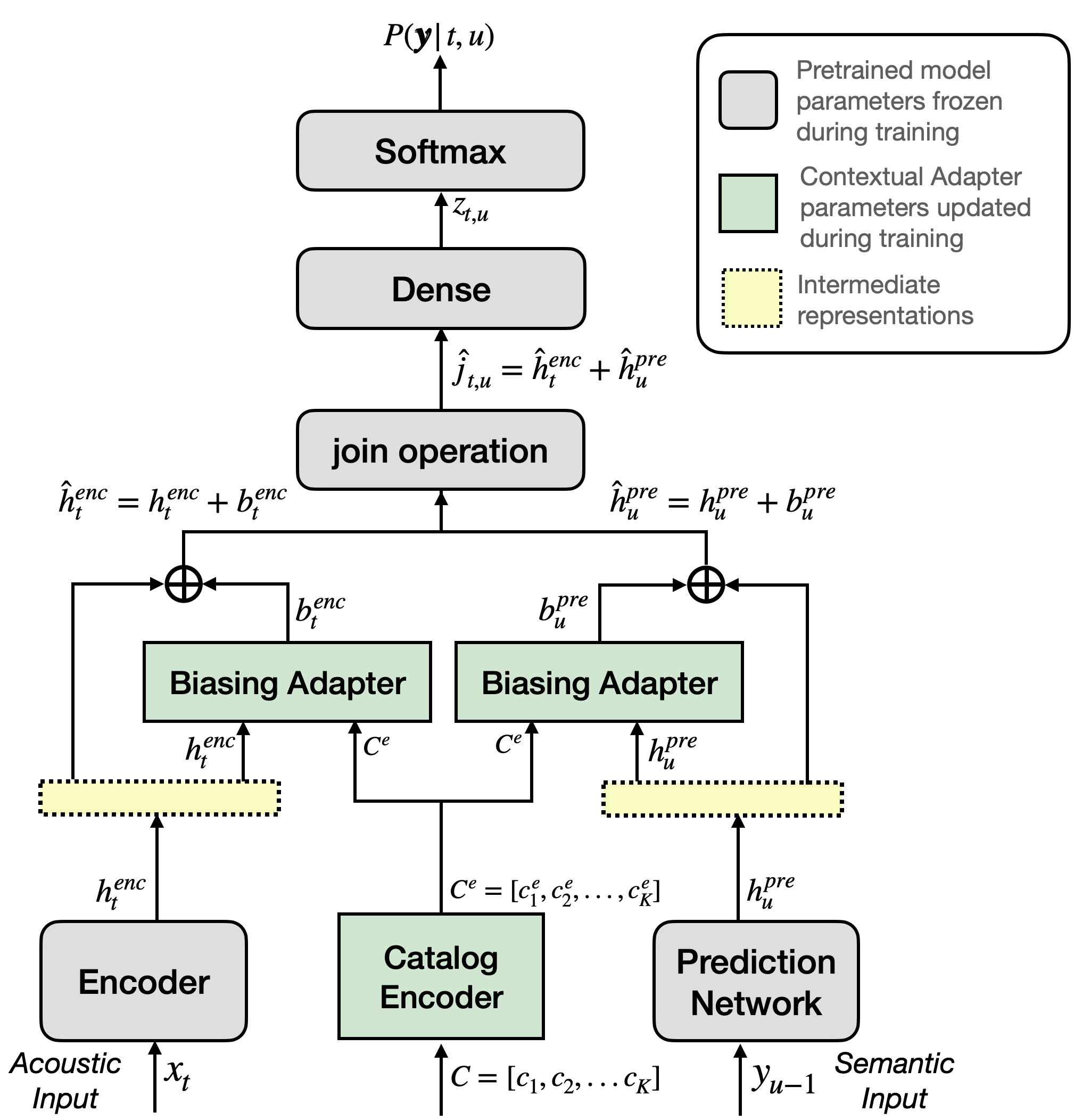
The biasing adapter adapts intermediate representations from the neural transducers by incorporating biasing information as shown in Figure 1 and 2. We propose cross-attention based biasing adapters (Figure 2 (b)) to attend over based on the input query . The query and the catalog entity embeddings are first projected via and to dimension . And the attention score for each catalog entity embedding is computed by the scaled dot product attention mechanism [23]:
The attention scores are used to compute a weighted sum of the value embeddings obtained by a linear projection of the catalog entity embeddings, which becomes the biasing vector, .
![[Uncaptioned image]](/html/2205.13660/assets/figs/joint_mha.png)
The biasing vectors are used to update the intermediate representations of a pretrained neural transducer. Note that all updates to intermediate representations are performed via element-wise additions (denoted by ). We investigate four biasing variants depending on the query being used for the biasing adapter (BA): (1) Enc Query: is provided as the query, and is adapted to produce :
| (2) |
(2) Pred Query: is the query and adapted to produce :
| (3) |
(3) Enc-Pred Query: Both and are adapted as in equations 2 and 3 before passing them to the joint network. (4) Joint Query: The result of the join operation, , is the query and is adapted to produce . This is used to update the joint representation before passing it through the activation and the dense layer.
3.3 Adapter Style Training
By design, our contextual ASR model is built by auxiliary training of contextual adapters. In this style of training, all network parameters, except the adapters (shown in green in Figure 1), are initialized with a pretrained model trained on large amounts of generic ASR data, without any contextextualization. The pretrained model parameters are then kept frozen, while the adapter modules are randomly initialized and trained from scratch. Since all the updates to intermediate representations are performed by element-wise additions, the pretrained model architecture can remain the same.
3.4 Handling multiple catalog types
Finally, our approach can be further extended to support multiple types of catalogs such as Proper Names, Device Names (eg. ‘Harry Potters lamp’ etc.) and/or Locations (eg. ‘bedroom’, ‘kitchen’ etc.). A shared catalog encoder is used to encode entities of different types. In order for the contextual adapters to distinguish between different catalog types and bias toward a specific one, we introduce a learnable ‘type_embedding’. Given the entity and it’s type where is the set of entity types, the embedding is computed as follows.
4 Experiments
4.1 Datasets and Evaluation Metrics
We use in-house voice assistant datasets with each utterance consisting of the audio and transcription randomly sampled from the VA traffic across more than 20 domains such as Communications, Weather, SmartHome, and Music. 114k hours of data are used to pre-train the baseline RNN-T and C-T models. For training the adapters, we use approximately 290 hours of data, containing a mix of specific and general training data (Mixed Dataset) in the ratio of (:1), where is a hyperparameter. Specific datasets contain utterances with mentions of proper names, device names and/or locations. General utterances are sampled from the original training data distribution. The training data is not associated with identifying information, but some utterances may contain personal information. Mixing a comparable proportion of specific and general utterances enables the adapters to learn when to or not to bias toward specific words. We evaluate our models and report results on two test sets - a 75 hour general dataset, and a 20 hour specific dataset 111there does not exist an equivalent, publicly available contextual dataset.
For our experiments, we report the relative word error rate reduction (WERR) on the general and specific sets, and the relative named entity word error rate reduction (NE-WERR) for contextual entity types. For WER, given a model A’s WER () and a baseline B’s WER (), the WERR of A over B is computed as NE-WERR is computed similarly and is used to demonstrate the improvement on contextual entities. Higher values indicate better performance.
4.2 Experimental Setup
We evaluate the contextual adapters with two pretrained neural transducer based ASR models, RNN-T and C-T.
Pretrained RNN-T and C-T. Both RNN-T and C-T are pretrained on a large 114k hour corpus. The input audio features are 64-dimensional LFBE features extracted every 10 ms with a window size of 25 ms and resulting in 192 feature dimensions per frame. Ground truth tokens are passed through a 4000 word-piece sentence piece tokenizer [21, 22]. The RNN-T encoder network consists of 5 LSTM layers with 736 units each with a time-reduction layer (downsampling factor of 2) at layer three. The C-T encoder network consists of 2 convolutional layers with kernel size=3, strides=2, and 128 filters, followed by a dense layer to project input features to 512 dimensions. They are then fed into 12 conformer blocks [19]. Each conformer block consists of a 512-node feed-forward layer, 1 transformer layer with 4 64-dim attention heads, 1 convolutional module with kernel size=32, and then feed-forward layer of 512 nodes. All the conformer blocks contain layer normalizations and residual links in between layers. All convolutions and attentions are computed on the current and previous audio frames to make it streamable. For both models, the prediction network consists of 2 LSTM layers with 736 units per layer. The outputs from the encoder and prediction network are projected through a feed-forward layer to 512 units. The joint network performs the join operation, which is a simple addition (). Additionally, we use a activation for the RNN-T model. Decoding is performed using the standard RNN-T/C-T beam search with a beam size of 8. The output vocabulary consists of 4000 word-pieces.
Contextual Adapter Configuration. The catalog encoder is a BiLSTM layer with 128 units (each for forward and backward LSTM) with an input size 64. The final output is projected to 64-dimensions. The biasing adapters project the query, key and values to 64-dimensions. The attention context vector obtained is projected to the same size as the encoder and/or prediction network or joint output sizes. For training the adapters, we use the Adam optimizer with learning rate 5e-4 trained to convergence with early stopping. We use a mix of Specific and General dataset in the ratio (=1.5:1), selected based on a hyperparameter search. The contextual adapters in total make up <500k parameters (<1.5% of the pretrained ASR model parameters). The maximum catalog size () is set to 300 during training to fit within memory. For experiments with multiple catalog types, we also concatenate a type embedding of size 8. We set the maximum catalog size to 300 for Proper Names, and 100 for Appliances and Device Location, respectively.
Baseline – Pretrained RNN-T/C-T. Our first baseline is the non-personalized pretrained RNN-T/C-T model as described previously.
Basline + SF – Pretrained RNN-T/C-T + Shallow Fusion. For the SF baseline, we build sub-word FSTs for the contextual information from user catalogs, and perform on-the-fly biasing during beam decoding, combining scores from the RNN-T model and the FST during lattice generation [24, 25]. We perform word-piece level biasing with weight-pushing, using subtractive costs to prevent incorrectly biased sub-words that do not form full words in the FST [5].
5 Results
| Model | RNN-T | C-T | ||||
|---|---|---|---|---|---|---|
| General | Proper Names | Proper Names | General | Proper Names | Proper Names | |
| WERR | NE-WERR | WERR | NE-WERR | |||
| Baseline | 0.00 | 0.00 | 0.00 | 0.00 | 0.00 | 0.00 |
| Baseline + SF | -3.87 | +21.84 | +27.70 | -3.02 | +24.22 | +38.12 |
| CA - Enc Query | -1.50 | +30.37 | +33.60 | -2.01 | +30.66 | +42.83 |
| CA - Pred Query | -1.45 | +12.43 | +13.30 | -2.42 | +11.13 | +23.34 |
| CA - Enc-Pred Query | -3.12 | +31.29 | +34.10 | -2.87 | +30.65 | +44.33 |
| CA - Joint Query | -2.69 | +26.24 | +29.00 | -1.14 | +30.28 | +42.83 |
| CA - Enc-Pred Query + SF | -4.43 | +36.17 | +39.70 | -2.92 | +34.95 | +46.68 |
Tables 1, 2, 3 present results for personalization in the Communications domain, where proper names (eg. contacts) are used for biasing. Note that the baseline pretrained models work well on the General set (below 10% absolute WER) while poorly on the Specific set (below 20% and above 10% absolute WER). We train contextual adapters with two types of neural transducers – RNN-T and C-T, and demonstrate that the approach is generic and applicable to this class of models. In Table 1, we compare contextual adapters with different query types on both – the general test set (General) and the specific Proper Name test set Proper Names. The proposed models outperform the baseline methods for all query types. Enc-Pred Query model achieves the greatest improvement on the Proper Names set (NE-WERR of 34.1% and 44.33% for RNN-T and C-T, respectively). Moreover, the degradation on the General set of our methods is smaller compared to SF (-1.14% vs -3.02% WERR for C-T). Interestingly, we found that adapting the encoder outputs (as in Enc and Enc-Pred Query) is more important than adapting only the prediction network outputs (Pred Query). Finally, we show that combining contextual adapters with SF, we obtain the most improvement on Proper Names test set (39.70% and 46.68% NE-WERR for RNN-T and C-T), showing that these two approaches are complementary to each other. We do notice a slighly higher degradation on the General set. We hypothesize that this is due to overbiasing from using both approaches.
Importance of Adapter-Style Training.
We observe that it is essential to freeze the base RNN-T parameters to obtain good improvements on proper names (Table 2).
Fine-tuning all parameters on the 290 hour Mixed dataset degrades the performance on the General set significantly (-19.23% WERR) resulting from catastrophic forgetting[26] as the base model parameters get updated. We hypothesize that this is due to the distribution shift in the Mixed Dataset causing the model to lose performance on the dataset it was original trained on (i.e the General dataset). Adapter style training can effectively reduce catastrophic forgetting (-19.23 vs -3.11 WERR). Furthermore, it outperforms full fine-tuning on the Proper Names set by a large margin +31.29% vs. +2.19% WERR.
| Training Type | General | Proper Names |
|---|---|---|
| Adapter Training (Base RNN-T Frozen) | -3.11 | +31.29 |
| Full fine-tuning (Base RNN-T Updated) | -19.23 | +2.19 |
Importance of the <no_bias> token and biasing adapters. With the best-performing contextual adapter model using Enc-Pred Query in Table 1, we see that removing the <no_bias> token results in a significant WER degradation (Table 3) on the General set (-15.31% vs -3.11% WERR). It indicates the <no_bias> token is essential to help the adapters learn when not to bias. Further, to verify if the biasing adapters really learn to attend towards the correct proper names, we train a contextual adapter with random word pieces in the catalog. We see a huge drop in WERR on the Proper Names set (31.29% to 6.82%) indicating that the biasing adapters have learned where to bias toward when the right proper names are provided.
| Ablations | General | Proper Names |
|---|---|---|
| Enc-Pred Query | -3.11 | +31.29 |
| without <no_bias> | -15.31 | +31.29 |
| with Random Catalog | -2.87 | +6.82 |
| Entity type | w/ TE | w/o TE |
|---|---|---|
| Appliance | +25.00 | +25.00 |
| Location | +29.17 | +29.17 |
| Proper Names | +38.66 | +27.53 |
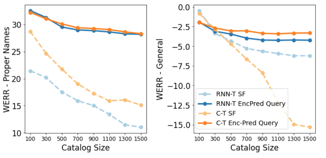
Impact of catalog sizes. We further evaluate the robustness of contextual adapters towards large catalogs where most entities are irrelevant and do not appear in the reference transcript. In Fig. 3, we show WERRs for the Enc-Pred Query variant over baseline RNN-T/C-T. In Proper Names set, our approach is more robust than SF scales better; the WERRs remain above 25% even at large sizes. The gap between SF and our approach increases as the catalog sizes increase. Additionally, our method degrades lesser on the General set when compared to SF as catalogs grow in size.
Handling multiple catalog types. Finally, we show that our method can handle multiple catalog types by incorporating the catalog type embedding (TE), and evaluated on 20 hours of contextual utterances for each entity type – Appliance, Location and Proper Names. As seen in Table 4, our method learns which type of catalog to bias and achieves consistent improvements not only for proper names, but also for Appliance and Location. Further, removing the TE degrades the performance on proper names showing it’s importance.
6 Conclusion
In this paper, we introduced contextual adapters to adapt pretrained RNN-T and C-T to improve speech recognition of contextual entities such as contact names, device names etc. While previous works have focused on training contextual models from scratch, our approach can adapt an already trained ASR model, by training only a small set of parameters. We also show that adapter-style training improves over shallow fusion baselines, while retaining the same flexibility as shallow fusion. Our approach improves by over 31% when compared to our baseline models on a dataset containing contextual utterances, while degrading less than 3.5% relative on the non-contextual utterances. We further demonstrate our model can handle multiple catalog types with the same kind of improvements.
References
- [1] Tara N Sainath, Rohit Prabhavalkar, Shankar Kumar, Seungji Lee, Anjuli Kannan, David Rybach, Vlad Schogol, Patrick Nguyen, Bo Li, Yonghui Wu, et al., “No need for a lexicon? evaluating the value of the pronunciation lexica in end-to-end models,” in 2018 IEEE International Conference on Acoustics, Speech and Signal Processing (ICASSP). IEEE, 2018, pp. 5859–5863.
- [2] Tony Bruguier, Fuchun Peng, and Françoise Beaufays, “Learning personalized pronunciations for contact names recognition,” 2016.
- [3] Golan Pundak, Tara N Sainath, Rohit Prabhavalkar, Anjuli Kannan, and Ding Zhao, “Deep context: end-to-end contextual speech recognition,” in 2018 IEEE spoken language technology workshop (SLT). IEEE, 2018, pp. 418–425.
- [4] Antoine Bruguier, Rohit Prabhavalkar, Golan Pundak, and Tara N Sainath, “Phoebe: Pronunciation-aware contextualization for end-to-end speech recognition,” in ICASSP 2019-2019 IEEE International Conference on Acoustics, Speech and Signal Processing (ICASSP). IEEE, 2019, pp. 6171–6175.
- [5] Aditya Gourav, Linda Liu, Ankur Gandhe, Yile Gu, Guitang Lan, Xiangyang Huang, Shashank Kalmane, Gautam Tiwari, Denis Filimonov, Ariya Rastrow, et al., “Personalization strategies for end-to-end speech recognition systems,” in ICASSP 2021-2021 IEEE International Conference on Acoustics, Speech and Signal Processing (ICASSP). IEEE, 2021, pp. 7348–7352.
- [6] Mahaveer Jain, Gil Keren, Jay Mahadeokar, Geoffrey Zweig, Florian Metze, and Yatharth Saraf, “Contextual rnn-t for open domain asr,” arXiv preprint arXiv:2006.03411, 2020.
- [7] Duc Le, Gil Keren, Julian Chan, Jay Mahadeokar, Christian Fuegen, and Michael L Seltzer, “Deep shallow fusion for rnn-t personalization,” in 2021 IEEE Spoken Language Technology Workshop (SLT). IEEE, 2021, pp. 251–257.
- [8] Duc Le, Mahaveer Jain, Gil Keren, Suyoun Kim, Yangyang Shi, Jay Mahadeokar, Julian Chan, Yuan Shangguan, Christian Fuegen, Ozlem Kalinli, et al., “Contextualized streaming end-to-end speech recognition with trie-based deep biasing and shallow fusion,” arXiv preprint arXiv:2104.02194, 2021.
- [9] Ding Zhao, Tara N. Sainath, David Rybach, Pat Rondon, Deepti Bhatia, Bo Li, and Ruoming Pang, “Shallow-Fusion End-to-End Contextual Biasing,” in Proc. Interspeech 2019, 2019, pp. 1418–1422.
- [10] Yanzhang He, Tara N Sainath, Rohit Prabhavalkar, Ian McGraw, Raziel Alvarez, Ding Zhao, David Rybach, Anjuli Kannan, Yonghui Wu, Ruoming Pang, et al., “Streaming end-to-end speech recognition for mobile devices,” in ICASSP 2019-2019 IEEE International Conference on Acoustics, Speech and Signal Processing (ICASSP). IEEE, 2019, pp. 6381–6385.
- [11] William Chan, Navdeep Jaitly, Quoc V. Le, and Oriol Vinyals, “Listen, attend and spell: A neural network for large vocabulary conversational speech recognition,” in ICASSP, 2016.
- [12] Jan Chorowski, Dzmitry Bahdanau, Dmitriy Serdyuk, Kyunghyun Cho, and Yoshua Bengio, “Attention-based models for speech recognition,” arXiv preprint arXiv:1506.07503, 2015.
- [13] Zhehuai Chen, Mahaveer Jain, Yongqiang Wang, Michael L Seltzer, and Christian Fuegen, “Joint grapheme and phoneme embeddings for contextual end-to-end asr.,” in INTERSPEECH, 2019, pp. 3490–3494.
- [14] Feng-Ju Chang, Jing Liu, Martin Radfar, Athanasios Mouchtaris, Maurizio Omologo, Ariya Rastrow, and Siegfried Kunzmann, “Context-aware transformer transducer for speech recognition,” ASRU, 2021.
- [15] Sylvestre-Alvise Rebuffi, Hakan Bilen, and Andrea Vedaldi, “Learning multiple visual domains with residual adapters,” arXiv preprint arXiv:1705.08045, 2017.
- [16] Sylvestre-Alvise Rebuffi, Hakan Bilen, and Andrea Vedaldi, “Efficient parametrization of multi-domain deep neural networks,” in Proceedings of the IEEE Conference on Computer Vision and Pattern Recognition, 2018, pp. 8119–8127.
- [17] Neil Houlsby, Andrei Giurgiu, Stanislaw Jastrzebski, Bruna Morrone, Quentin De Laroussilhe, Andrea Gesmundo, Mona Attariyan, and Sylvain Gelly, “Parameter-efficient transfer learning for nlp,” in International Conference on Machine Learning. PMLR, 2019, pp. 2790–2799.
- [18] Alex Graves, “Sequence transduction with recurrent neural networks,” arXiv preprint arXiv:1211.3711, 2012.
- [19] Anmol Gulati, James Qin, Chung-Cheng Chiu, Niki Parmar, Yu Zhang, Jiahui Yu, Wei Han, Shibo Wang, Zhengdong Zhang, Yonghui Wu, et al., “Conformer: Convolution-augmented transformer for speech recognition,” arXiv preprint arXiv:2005.08100, 2020.
- [20] Bo Li, Anmol Gulati, Jiahui Yu, Tara N Sainath, Chung-Cheng Chiu, Arun Narayanan, Shuo-Yiin Chang, Ruoming Pang, Yanzhang He, James Qin, et al., “A better and faster end-to-end model for streaming asr,” in ICASSP 2021-2021 IEEE International Conference on Acoustics, Speech and Signal Processing (ICASSP). IEEE, 2021, pp. 5634–5638.
- [21] Rico Sennrich, Barry Haddow, and Alexandra Birch, “Neural machine translation of rare words with subword units,” in ACL, 2016.
- [22] Taku Kudo, “Subword regularization: Improving neural network translation models with multiple subword candidates,” arXiv preprint arXiv:1804.10959, 2018.
- [23] Ashish Vaswani, Noam Shazeer, Niki Parmar, Jakob Uszkoreit, Llion Jones, Aidan N Gomez, L ukasz Kaiser, and Illia Polosukhin, “Attention is all you need,” in Advances in Neural Information Processing Systems, I. Guyon, U. V. Luxburg, S. Bengio, H. Wallach, R. Fergus, S. Vishwanathan, and R. Garnett, Eds. 2017, vol. 30, Curran Associates, Inc.
- [24] David Rybach, Michael Riley, and Johan Schalkwyk, “On lattice generation for large vocabulary speech recognition,” in 2017 IEEE Automatic Speech Recognition and Understanding Workshop (ASRU). IEEE, 2017, pp. 228–235.
- [25] Ding Zhao, Tara N Sainath, David Rybach, Pat Rondon, Deepti Bhatia, Bo Li, and Ruoming Pang, “Shallow-fusion end-to-end contextual biasing.,” in Interspeech, 2019, pp. 1418–1422.
- [26] James Kirkpatrick, Razvan Pascanu, Neil Rabinowitz, Joel Veness, Guillaume Desjardins, Andrei A Rusu, Kieran Milan, John Quan, Tiago Ramalho, Agnieszka Grabska-Barwinska, et al., “Overcoming catastrophic forgetting in neural networks,” Proceedings of the national academy of sciences, vol. 114, no. 13, pp. 3521–3526, 2017.