Topological indices in Random Spiro Chains

Abstract: Let $G=(V(G),E(G))$ denote a graph, many important topological indices can be defined as

$TI(G)=\sum_{v\in V(G)}h(d_{v})^{a}$,

or

$TI(G)=\sum_{vu\in E(G)}f(d_{v},d_{u})^{a}$.

In this paper, we study these kinds of topological indices in random spiro chains via a martingale approach. In which their explicit analytical expressions of the exact distribution, expected value and variance are obtained. As $n$ goes to $\infty$, the asymptotic normality of topological indices of a random spiro chain is established through the Martingale Central Limit Theorem. In particular, we compute the Nirmala, Sombor, Randić and Zagreb index for a random spiro chain along with their comparative analysis.

1 Introduction

A graph $G$ is determined by two sets $(V(G),E(G))$, the set of nodes ($V(G)$) and edges ($E(G)$). The edges and nodes are interpreted according to the problem to be modeled. In particular, a molecular graph is a simple graph such that its vertices correspond to the atoms and the edges to the bonds of a molecule, where a simple graph is a graph without directed, weighted or multiple edges, and without self-loops. Topological indices numerically quantify aspects of these graphs for multiple purposes, such as sparseness, regularity, and centrality. In addition, the first and second Zagreb indices appeared for the first time in [Gutman and TrinajstićGutman and Trinajstić1972], then it is defined in [RandicRandic1975] the Randić index. These indices are mostly historical and well-known indices which have been widely used to predict the properties of compounds; since have been proved to have a wide range of functions as topological variables supported by chemical experiment data. In [GutmanGutman2021], a novel topological index was introduced via a geometric approach, named Sombor index defined as

$SO(G)=\displaystyle\sum_{uv\in E(G)}\sqrt{\left(d_{u}\right)^{2}+\left(d_{v}\right)^{2}}$,

where $d_{v}$ is the degree of a vertex $v$. Nowadays, several graph invariants related to the Sombor index have been presented. For example, in [KulliKulli2021], Kulli introduced the Nirmala index of a graph $G$ as follows

$$N(G)=\displaystyle\sum_{uv\in E(G)}\sqrt{d_{u}+d_{v}}.$$ (1)

Recent work on the Nirmala index can be consulted in [Gutman and KulliGutman and Kulli2021], [Kulli, Chaluvaraju, and AshaKulli et al.2021] and [Gutman, Kulli, and RedzepovicGutman et al.2021]. In general, topological indices that can be constructed for static and random graphs represent a major part of the current research in mathematical chemistry and chemical graph theory.

On the other hand, the martingale theory is a very powerful and deep mathematical tool. The concept was introduced by Paul Lévy in 1934, and was given its name in 1939 by J. André Ville. The development of a whole theory around martingales is due to Joseph L. Doob. Nowadays, the concept of martingales is well-known. In particular, there are martingale central limit theorems, which give conditions under which the whole process is approximately normally distributed. Actually, in [Feng and HuFeng and Hu2015] and [KazemiKazemi2021] the authors used a martingale approach to study topological indices, such as the Zagreb, Gordon-Scantlebury and Platt indices.

In [Li, Shi, and GaoLi et al.2021], [Raza and ImranRaza and Imran2021], [RazaRaza2021], [Fang, You, and LiuFang et al.2021], [JahanbaniJahanbani2020], [Wei, Ke, and HaoWei et al.2018], [RazaRaza2020], [DengDeng2012] and [Zhang, You, Liu, and HuangZhang et al.2021] the authors studied topological indices in random chains. In particular, spiro compounds are an important class of cycloalkanes in organic chemistry. The derivatives of spiros are fairly often seen chemicals, which may be utilized in organic synthesis, drug synthesis, heat exchanger, etc. Motivated for the above information, we make researches on topological indices in random spiro chains. In this paper, our goal is to associate a martingale to the topological index, so that, the properties that can be deduced from the martingale are useful to show those of the topological index. We first establish exact formulas for the expected value, variance and the exact distribution of topological indices in random spiro chains. Moreover, we find a general result for the asymptotic distribution via this approach. Finally, as applications, using the Nirmala, Sombor, Randić and Zagreb index, the results are given for random spiro chains (see in Definition 1).

Definition 1.

The random spiro chain $RSC_{n}=RSC\left(n,p_{1},p_{2},p_{3}\right)$ with $n$ hexagons is constructured by the following way:

• $RSC_{1}$ is a hexagon and $RSC_{2}$ contains two hexagons, see Figure 1.

• For every $n>2,RSC_{n}$ is constructured by attaching one hexagon to $RSC_{n-1}$ in three ways, resulted in $RSC_{n}^{1},RSC_{n}^{2},RSC_{n}^{3}$ with probability $p_{1},p_{2}$ and $p_{3}$ respectively, where $0<p_{i}<1$ and $p_{1}+p_{2}+p_{3}=1$, see Figure 2.

Figure 1: The graphs of $RSC_{1}$ and $RSC_{2}$.

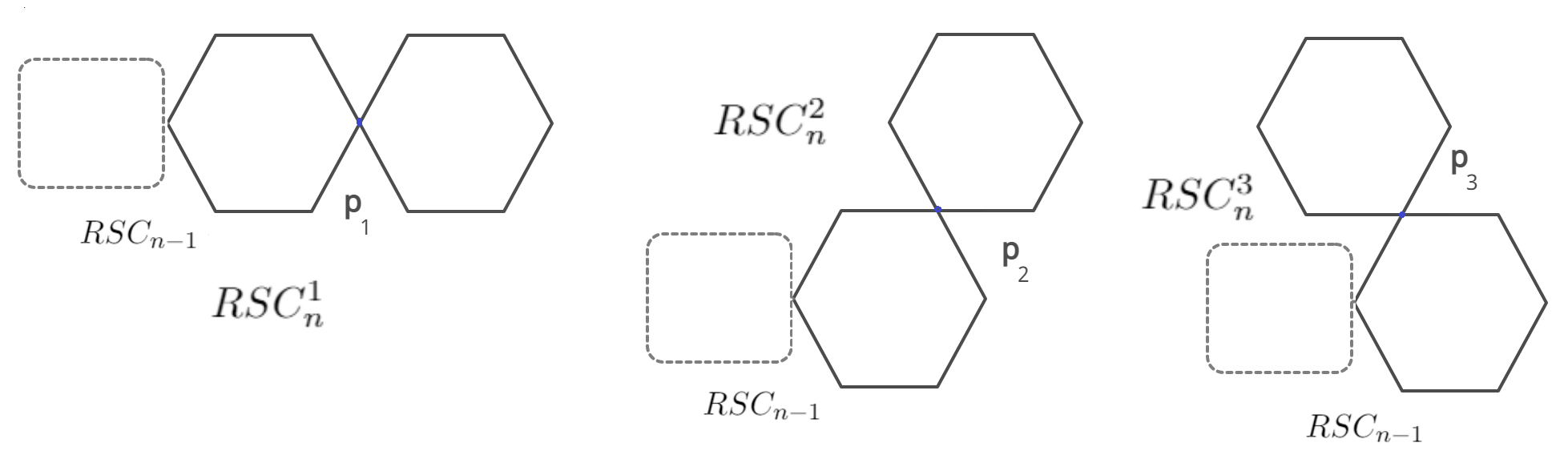
Figure 2: The three link ways for $RSC_{n}(n>2)$.

2 Topological indices in random spiro chains.

Let $G=(V(G),E(G))$, many important topological indices can be defined as

$$TI(G)=\displaystyle\sum_{v\in V(G)}h(d_{v})^{a},$$ (2)

or

$$TI(G)=\displaystyle\sum_{vu\in E(G)}f(d_{v},d_{u})^{a},$$ (3)

where $a\in\mathbb{R}$, $h:\{1,2,\dots\}\rightarrow(0,\infty)$ and $f:\{1,2,\dots\}\times\{1,2,\dots\}\rightarrow(0,\infty)$ is any symmetric function. The main topological indices of the form (2) and (3) are:

• If $h(t)=t$ and $a=2$ then $TI(G)$ is the first Zagreb index.

• If $h(t)=t$ and $a=-1$ then $TI(G)$ is the inverse degree index.

• If $h(t)=t$ and $a=3$ then $TI(G)$ is the forgotten index.

• If $h(t)=t$ and $a\in\mathbb{R}$ then $TI(G)$ is the variable first Zagreb index.

• If $f(x,y)=xy$ and $a=1$ then $TI(G)$ is the second Zagreb index.

• If $f(x,y)=xy$ and $a=-1/2$ then $TI(G)$ is the usual Randić index.

• If $f(x,y)=x+y$ and $a=-1/2$ then $TI(G)$ is the sum-connectivity index.

• If $f(x,y)=x+y$ and $a=-1$ then $2TI(G)$ is the harmonic index.

• If $f(x,y)=x+y$ and $a\in\mathbb{R}$ then $TI(G)$ is the variable sum-connectivity index.

Remark 1.

Note that the Nirmala index (1) is the reverse version of the sum-connectivity index. In addition, the Nirmala index is the variable sum-connectivity index, for $a=1/2$.

Theorem 1.

Let $RSC_{n}=RSC\left(n,p_{1},p_{2},p_{3}\right)$ with $n\geq 2$ be a random spiro chain. Then

$$\mathbb{E}(TI_{n})=TI_{2}+\alpha(n-2),$$

$$V(TI_{n})=(\beta-\alpha^{2})(n-2),$$

where $i=1,2,3$, $TI_{n}=TI(RSC_{n})$, $TI_{n,i}=TI(RSC_{n}^{i})$, $\alpha_{i}=TI_{3,i}-TI_{2}$, $\alpha=\displaystyle\sum_{i=1}^{3}\alpha_{i}p_{i}$ and $\beta=\displaystyle\sum_{i=1}^{3}\alpha_{i}^{2}p_{i}$.

Proof.

Let $n\geq 3$ and $L_{n}$ denote a random variable with range $\{1,2,3\}$ and let $p_{i}=\mathbb{P}(L_{n}=i)$ and $L_{2}$ denote the initial link, i.e., $L_{n}$ denote the link selected at time $n$. Note that, at time $n-1$ we have

$\underbrace{\underbrace{HL_{2}H}_{{RSC_{2}}}L_{3}HL_{4}HL_{5}\dots L_{n-1}H}_{{RSC_{n-1}}}.$

Then, at time $n$, we obtain

$\underbrace{\underbrace{\underbrace{HL_{2}H}_{{RSC_{2}}}L_{3}HL_{4}HL_{5}\dots L_{n-1}H}_{{RSC_{n-1}}}L_{n}H}_{{RSC_{n}}}.$

Therefore, we must pay attention to the change in the calculation of the topological index by joining $H$ with $H$ via $L_{n}$. Let $n\geq 3$ and $i=1,2,3$, then based on this approach, by the definition of a random spiro chain and $TI(G)$ in Equation (2) and (3), we obtain the following almost-sure recursive relation between $TI_{n-1}$ and $TI_{n}$, conditional on the event that the at time $n$ the link $i$ is selected and $\mathbb{F}_{n-1}$

$$TI_{n,i}-TI_{n-1}=TI_{3,i}-TI_{2},$$

where $\mathbb{F}_{n-1}$ denotes the $\sigma$-field generated by the history of the growth of the random spiro chain in the first $n-1$ stages. Now, we take the expectation with respect to $L_{n}$ to get,

$$\mathbb{E}(TI_{n}\mid\mathbb{F}_{n-1}) = \displaystyle\sum_{i=1}^{3}(TI_{n-1}+\alpha_{i})p_{i}$$

$$= TI_{n-1}+\sum_{i=1}^{3}\alpha_{i}p_{i},$$

where, $\alpha_{i}=TI_{3,i}-TI_{2}$. Then, taking expectation, we obtain a recurrence relationship for $\mathbb{E}(TI_{n})$,

$$\mathbb{E}(TI_{n})=\mathbb{E}(TI_{n-1})+\sum_{i=1}^{3}\alpha_{i}p_{i}.$$ (4)

We solve Equation $(\ref{e2})$ with the initial value $\mathbb{E}(TI_{2})=TI_{2}$ and we obtain the result stated in the theorem,

$$\mathbb{E}(TI_{n})=TI_{2}+\alpha(n-2),$$

where $\alpha=\displaystyle\sum_{i=1}^{3}\alpha_{i}p_{i}$. The expressions for $\mathbb{E}(TI^{2}_{n})$ follow in a similar manner,

$$\mathbb{E}(TI^{2}_{n}\mid\mathbb{F}_{n-1}) = \displaystyle\sum_{i=1}^{3}(TI_{n-1}+\alpha_{i})^{2}p_{i}$$

$$= \displaystyle\sum_{i=1}^{3}TI^{2}_{n-1}p_{i}+2TI_{n-1}\alpha_{i}p_{i}+\alpha_{i}^{2}p_{i}$$

$$= TI^{2}_{n-1}+2TI_{n-1}\alpha+\beta,$$

where $\beta=\displaystyle\sum_{i=1}^{3}\alpha_{i}^{2}p_{i}$, thus

$$\mathbb{E}(TI^{2}_{n}) = \mathbb{E}(TI^{2}_{n-1})+2\alpha\mathbb{E}(TI_{n-1})+\beta$$

$$= \mathbb{E}(TI^{2}_{n-1})+2\alpha TI_{2}+2\alpha^{2}(n-3)+\beta,$$

with $\mathbb{E}(TI^{2}_{2})=TI^{2}_{2}$, then iterating, it is obtained that

$\mathbb{E}(TI^{2}_{n})=TI^{2}_{2}+(2\alpha TI_{2}+\beta)(n-2)+(n-3)(n-2)\alpha^{2}.$

The variance of $TI_{n}$ is obtained immediately by taking the difference between $\mathbb{E}(TI^{2}_{n})$ and $\mathbb{E}(TI_{n})^{2}$,

$$V(TI_{n}) = \beta(n-2)+\left((n-2)(n-3)-(n-2)^{2}\right)\alpha^{2}$$

$$= (\beta-\alpha^{2})(n-2),$$

proving the theorem. ∎

Note that $\beta-\alpha^{2}=0$ if and only if $\alpha_{1}=\alpha_{2}=\alpha_{3}$ if and onl if $TI_{n}=TI_{2}+\alpha(n-2)$ a.s. with $n\geq 2$ (a deterministic sequence). Now, we exploit a martingale formulation to investigate the asymptotic behavior of $TI_{n}$ when $\beta-\alpha^{2}>0$. The key idea is to consider a transformation $M_{n}$ and we require that the transformed random variables form a martingale in the next proposition.

Proposition 1.

For $n\geq 2$, $\{M_{n}=TI_{n}-\alpha(n-2)\}_{n}$ is a martingale with respect to $\mathbb{F}_{n}$.

Proof.

Firstly, observe that $\mathbb{E}(|M_{n}|)<+\infty$. Then, by Theorem 1,

$$\mathbb{E}\left(TI_{n}-\alpha(n-2)\mid\mathbb{F}_{n-1}\right) =\mathbb{E}\left(TI_{n}\mid\mathbb{F}_{n-1}\right)-\alpha(n-2)$$

$$=TI_{n-1}+\alpha-\alpha(n-2)$$

$$=TI_{n-1}-\alpha(n-3).$$

The proof is completed.

∎

We use the notation $\stackrel{{\scriptstyle D}}{{\longrightarrow}}$ to denote convergence in distribution and $\stackrel{{\scriptstyle P}}{{\longrightarrow}}$ to denote convergence in probability. The random variable $\mathrm{N}\left(\mu,\sigma^{2}\right)$ appears in the following theorem for the normal distributed with mean $\mu$ and variance $\sigma^{2}$.

Theorem 2.

As $n\rightarrow\infty$,

$\frac{TI_{n}-(n-2)\alpha}{\sqrt{n}}\stackrel{{\scriptstyle D}}{{\longrightarrow}}N(0,\beta-\alpha^{2})$.

Proof.

Note that, for $j\geq 3$ and $i=1,2,3$, we have

$|\nabla M_{j}|=|\nabla TI_{j}-\alpha|\leq 2~{}\underset{i}{max}\{|\alpha_{i}|\}$,

where $\nabla M_{j}=M_{j}-M_{j-1}$ and $\nabla TI_{j}=TI_{j}-TI_{j-1}$. Then, as $n$ goes to $\infty$

$\displaystyle\lim_{n\rightarrow\infty}\frac{\left|\nabla M_{j}\right|}{\sqrt{n}}=0$.

That is, given $\varepsilon>0$, there exists an $n_{0}(\varepsilon)>0$ such that, the sets $\left\{|\nabla M_{j}|>\varepsilon\sqrt{n}\right\}$ are empty for all $n>n_{0}(\varepsilon)$. In what follows, we conclude that

$U_{n}:=\frac{1}{n}\displaystyle\sum_{j=3}^{n}\mathbb{E}\left(\left(\nabla M_{j}\right)^{2}\mathbb{I}_{\left\{|\nabla M_{j}|>\varepsilon\sqrt{n}\right\}}\mid\mathbb{F}_{j-1}\right),$

converges to 0 almost surely, hence, $U_{n}\stackrel{{\scriptstyle P}}{{\longrightarrow}}0$. As a result, the Lindeberg’s condition is verified. Next, the conditional variance condition is given by

$$V_{n}:=\frac{1}{n}\sum_{j=3}^{n}\mathbb{E}\left(\left(\nabla M_{j}\right)^{2}\mid\mathbb{F}_{j-1}\right)\stackrel{{\scriptstyle P}}{{\longrightarrow}}\beta-\alpha^{2}.$$

Note that,

$$\frac{1}{n}\sum_{j=3}^{n}\mathbb{E}\left(\left(\nabla M_{j}\right)^{2}\mid\mathbb{F}_{j-1}\right)= \frac{1}{n}\sum_{j=3}^{n}\mathbb{E}\left((\nabla TI_{j}-\alpha)^{2}\mid\mathbb{F}_{j-1}\right)$$

$$= \frac{1}{n}\sum_{j=3}^{n}\sum_{i=1}^{3}(\alpha_{i}-\alpha)^{2}p_{i}$$

$$= \frac{n-2}{n}\sum_{i=1}^{3}(\alpha_{i}-\alpha)^{2}p_{i}.$$

By the Martingale Central Limit Theorem [Hall and HeydeHall and Heyde2014], we thus obtain the stated result, since

$$\sum_{i=1}^{3}(\alpha_{i}-\alpha)^{2}p_{i}= \sum_{i=1}^{3}\alpha_{i}^{2}p_{i}-2\alpha\sum_{i=1}^{3}\alpha_{i}p_{i}+\alpha^{2}$$

$$= \beta-\alpha^{2}.$$

∎

Then we may use Theorem 2 to find the following result.

Corollary 1.

As $n\rightarrow\infty$,

$\frac{TI_{n}-\mathbb{E}(TI_{n})}{\sqrt{V(TI_{n})}}\stackrel{{\scriptstyle D}}{{\longrightarrow}}N(0,1)$.

The following theorem gives further details on the distribution for topological indices in random spiro chains. Here, $M_{R}(\cdot)$ denotes the moment generating function of a random variable $R$.

Theorem 3.

Let $RSC_{n}$ with $n\geq 2$ be a random spiro chain. Then,

$TI_{n}=TI_{2}+a^{T}X$,

where $a^{T}=(\alpha_{1},\alpha_{2},\alpha_{3})$ and $X=(X_{1},X_{2},X_{3})$ is a multinomial random variable with parameters $n-2$ and $(p_{1},p_{2},p_{3})$.

Proof.

Let $t\in\mathbb{R}$, note that,

$$\mathbb{E}\left(e^{tTI_{n}}\mid\mathbb{F}_{n-1}\right)= \sum_{i=1}^{3}e^{tTI_{n-1}}e^{t\alpha_{i}}p_{i}$$

$$= ~{}e^{tTI_{n-1}}\sum_{i=1}^{3}e^{t\alpha_{i}}p_{i}.$$

Thus, we can conclude that

$M_{TI_{n}}(t)=M_{TI_{n-1}}(t)\displaystyle\sum_{i=1}^{3}e^{t\alpha_{i}}p_{i}.$

We may therefore write,

$$M_{TI_{n}}(t)= M_{TI_{2}}(t)\left(\sum_{i=1}^{3}e^{t\alpha_{i}}p_{i}\right)^{n-2}$$

$$= M_{TI_{2}}(t)M_{X}(\alpha_{1}t,\alpha_{2}t,\alpha_{3}t)$$

$$= M_{TI_{2}}(t)M_{a^{T}X}(t),$$

which completes the proof. ∎

It is useful to note that the approximation given in Corollary 1 is identical to the one obtained by the following method. Let $n\geq 2$, by Theorem 3 we have that

$TI_{n}=TI_{2}+a^{T}X$.

It follows from the Central Limit Theorem to the case of random vectors [Severini et al.Severini et al.2012] that $X$ is asymptotically distributed according to a multivariate normal distribution with mean $\mathbb{E}(X)$ and covariance matrix $V(X)$. Consequently, $a^{T}X$ is asymptotically distributed according to a normal distribution with mean $a^{T}\mathbb{E}(X)$ and variance $a^{T}V(X)a$. Then, as $n$ goes to $\infty$

$\frac{TI_{n}-TI_{2}-a^{T}\mathbb{E}(X)}{\sqrt{a^{T}V(X)a}}=\frac{TI_{n}-\mathbb{E}(TI_{n})}{\sqrt{V(TI_{n})}}\xrightarrow{D}N(0,1)$.

3 Interpretation of the results and examples.

The conclusion of Section 2 can be stated as follows.

Theorem 4.

Let $RSC_{n}$ with $n\geq 2$ be a random spiro chain and $a\in\mathbb{R}$. Then

$TI(G)=\displaystyle\sum_{v\in V(G)}h\left(d_{v}\right)^{a}=2h(2)^{a}-h(4)^{a}+(4h(2)^{a}+h(4)^{a})n$,

and

$TI(G)=\displaystyle\sum_{vu\in E(G)}f\left(d_{v},d_{u}\right)^{a}=A+BX+Cn$,

$\mathbb{E}(TI_{n})=A+(Bp_{1}+C)n-2Bp_{1}$,

$V(TI_{n})=B^{2}p_{1}(1-p_{1})(n-2)$,

where $A=4f\left(2,2\right)^{a}-4f\left(2,4\right)^{a}$, $B=f\left(2,2\right)^{a}-2f\left(2,4\right)^{a}+f\left(4,4\right)^{a}$, $C=2f\left(2,2\right)^{a}+4f\left(2,4\right)^{a}$ and $X$ has a binomial distribution with parameters $n-2$ and $p_{1}$.

Proof.

As can be seen from the results obtained in Section 2, we need to find $TI_{2}$ and $\alpha_{i}$ with $i=1,2,3$. By the definition of $TI_{n}$ in Equation (2), $RSC_{2}$ and $RSC_{3}^{i}$, we have that,

$TI_{2}=10h(2)^{a}+h(4)^{a}$,

$T_{3,1}=T_{3,2}=T_{3,3}=14h(2)^{a}+2h(4)^{a}$.

Then,

$\alpha_{1}=\alpha_{2}=\alpha_{3}=4h(2)^{a}+h(4)^{a}$.

On the other hand, by the definition of $TI_{n}$ in Equation (3), it follows that,

$TI_{2}=8f(2,2)^{a}+4f(2,4)^{a}$,

$T_{3,1}=T_{3,2}=10f(2,2)^{a}+8f(2,4)^{a}$,

$T_{3,3}=11f(2,2)^{a}+6f(2,4)^{a}+f(4,4)^{a}$.

Then,

$\alpha_{1}=\alpha_{2}=2f(2,2)^{a}+4f(2,4)^{a}$,

$\alpha_{3}=3f(2,2)^{a}+2f(2,4)^{a}+f(4,4)^{a}$.

In each case, applying Theorem 1, 2 and 3, we verify the results. ∎

Remark 2.

Note that if $TI(G)=\displaystyle\sum_{v\in\in V(G)}h(d_{v})^{a}$ then $TI_{n}$ is a deterministic sequence and if $TI(G)=\displaystyle\sum_{vu\in E(G)}f(d_{v},d_{u})^{a}$, we have that $TI_{n}=TI_{2}+\alpha_{1}(n-2)$ with $n\geq 2$ (a deterministic sequence) if and only if $f(2,2)^{a}+f(4,4)^{a}=2f(2,4)^{a}$. In particular, if $a=1$ then taking $f(x,y)=x^{\theta}+y^{\theta}$ with $\theta\in\mathbb{R}$, it is verified that $f(2,2)+f(4,4)=2f(2,4)$; which make sense, since $TI(G)=\displaystyle\sum_{vu\in E(G)}d_{u}^{\theta}+d_{v}^{\theta}=\displaystyle\sum_{v\in E(G)}d_{v}^{\theta+1}$

Now, in order to apply Theorem 4, we present the following corollaries.

Corollary 2.

Let $RSC_{n}=RSC\left(n,p_{1},p_{2},p_{3}\right)$ be a random spiro chain and $N_{n}$ be the Nirmala index of a $RSC_{n}$, with $n\geq 2$. Then

$$N_{n}=8-4\sqrt{6}+(2-2\sqrt{6}+2\sqrt{2})X+(4+4\sqrt{6})n,$$

$$\mathbb{E}\left(N_{n}\right)=8-4\sqrt{6}+\left((2-2\sqrt{6}+2\sqrt{2})p_{1}+4+4\sqrt{6}\right)n-2(2-2\sqrt{6}+2\sqrt{2})p_{1},$$

$$V\left(N_{n}\right)=(2-2\sqrt{6}+2\sqrt{2})^{2}p_{1}\left(1-p_{1}\right)(n-2),$$

$$\frac{N_{n}-\mathbb{E}\left(N_{n}\right)}{\sqrt{V\left(N_{n}\right)}}\xrightarrow{D}N(0,1),$$

where $X$ has a binomial distribution with parameters $n-2$ and $p_{1}$.

Corollary 3.

Let $RSC_{n}=RSC\left(n,p_{1},p_{2},p_{3}\right)$ be a random spiro chain and $M1_{n}$ be the first Zagreb index of a $RSC_{n}$, with $n\geq 2$. Then

$$M1_{n}=32n-8.$$ (5)

Corollary 4.

Let $RSC_{n}=RSC\left(n,p_{1},p_{2},p_{3}\right)$ be a random spiro chain and $R_{n}$ be the Randić index of a $RSC_{n}$, with $n\geq 2$. Then

$$R_{n}=2-\sqrt{2}+(3/4-\sqrt{2}/2)X+(1+\sqrt{2})n,$$

$$\mathbb{E}\left(R_{n}\right)=2-\sqrt{2}+\left((3/4-\sqrt{2}/2)p_{1}+1+\sqrt{2}\right)n+(\sqrt{2}-3/2)p_{1},$$ (6)

$$V\left(R_{n}\right)=(3/4-\sqrt{2}/2)^{2}p_{1}\left(1-p_{1}\right)(n-2),$$

$$\frac{R_{n}-\mathbb{E}\left(R_{n}\right)}{\sqrt{V\left(R_{n}\right)}}\xrightarrow{D}N(0,1),$$

where $X$ has a binomial distribution with parameters $n-2$ and $p_{1}$.

Corollary 5.

Let $RSC_{n}=RSC\left(n,p_{1},p_{2},p_{3}\right)$ be a random spiro chain and $S_{n}$ be the Sombor index of a $RSC_{n}$, with $n\geq 2$. Then

$$S_{n}=8\sqrt{2}-8\sqrt{5}+(6\sqrt{2}-4\sqrt{5})X+(4\sqrt{2}+8\sqrt{5})n,$$

$$\mathbb{E}\left(S_{n}\right)=8\sqrt{2}-8\sqrt{5}+\left((6\sqrt{2}-4\sqrt{5})p_{1}+4\sqrt{2}+8\sqrt{5}\right)n-2(6\sqrt{2}-4\sqrt{5})p_{1},$$

$$V\left(S_{n}\right)=(6\sqrt{2}-4\sqrt{5})^{2}p_{1}\left(1-p_{1}\right)(n-2),$$

$$\frac{S_{n}-\mathbb{E}\left(S_{n}\right)}{\sqrt{V\left(S_{n}\right)}}\xrightarrow{D}N(0,1),$$

where $X$ has a binomial distribution with parameters $n-2$ and $p_{1}$.

Corollary 6.

Let $RSC_{n}=RSC\left(n,p_{1},p_{2},p_{3}\right)$ be a random spiro chain and $M2_{n}$ be the second Zagreb index of a $RSC_{n}$, with $n\geq 2$. Then

$$M2_{n}=4X+40n-16,$$

$$\mathbb{E}\left(M2_{n}\right)=\left(4p_{1}+40\right)n-8p_{1}-16,$$ (7)

$$V\left(M2_{n}\right)=16p_{1}\left(1-p_{1}\right)(n-2),$$

$$\frac{M2_{n}-\mathbb{E}\left(M2_{n}\right)}{\sqrt{V\left(M2_{n}\right)}}\xrightarrow{D}N(0,1),$$

where $X$ has a binomial distribution with parameters $n-2$ and $p_{1}$.

Remark 3.

In fact, we can see that (5) and (6) are obtained in [JahanbaniJahanbani2020]. Also, we can see that Corollary 5 and (7) are obtained in [Zhang, You, Liu, and HuangZhang et al.2021] and [RazaRaza2020], respectively.

Remark 4.

For $n\geq 2$ and $p_{1}\in(0,1)$, it follows from Corollary 2, 3, 4, 5 and 6 that

$\mathbb{E}(R_{n})\leq\mathbb{E}(N_{n})\leq\mathbb{E}(S_{n})\leq\mathbb{E}(M1_{n})\leq\mathbb{E}(M2_{n})$ (see Figure 3),

$V(R_{n})\leq V(N_{n})\leq V(S_{n})\leq V(M2_{n})$.

Figure 3: Difference between $\mathbb{E}(R_{n}),\mathbb{E}(N_{n}),\mathbb{E}(S_{n}),\mathbb{E}(M1_{n})$ and $\mathbb{E}(M2_{n})$.

Finally, we conduct a numerical experiment to support the asymptotic behaviors developed in Corollaries 2, 4, 5 and 6. Given a fixed $p_{1}\in(0,1)$, in each case, we independently generate $5,000$ replications of a random spiro chain after $n=10,000$ evolutionary steps. For each simulated random spiro chain, its topological index is computed. The histogram of the sample data with a normal approximation curve are given in Figure 4, 5, 6 and 7.

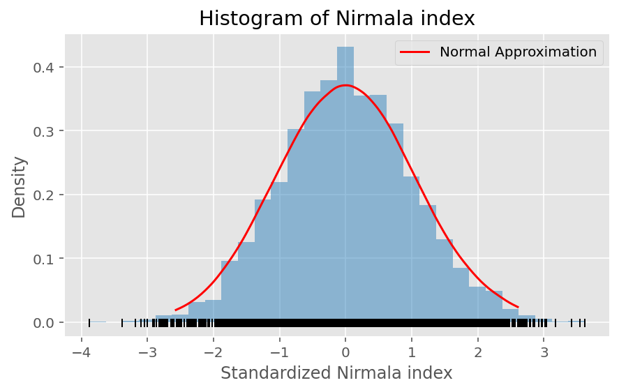
Figure 4: Histogram of the standardized Nirmala index of $5,000$ independently generated random spiro chains with $n=10,000$; the thick red curve is the estimated density of the sample.

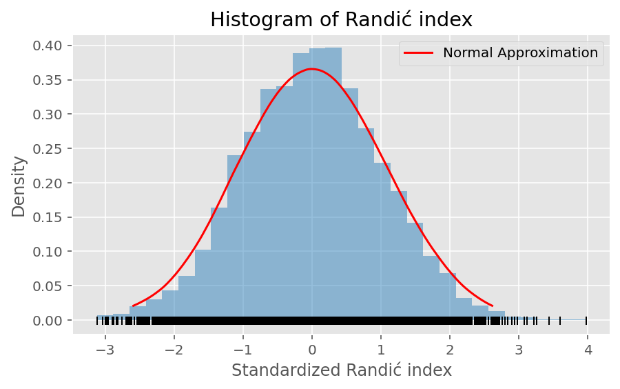
Figure 5: Histogram of the standardized Randić index of $5,000$ independently generated random spiro chains with $n=10,000$; the thick red curve is the estimated density of the sample.

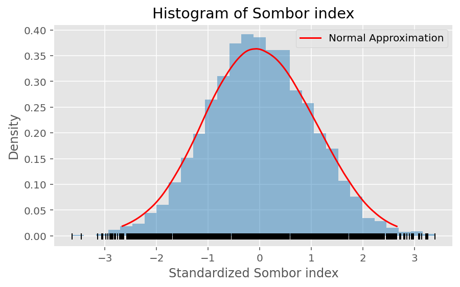
Figure 6: Histogram of the standardized Sombor index of $5,000$ independently generated random spiro chains with $n=10,000$; the thick red curve is the estimated density of the sample.

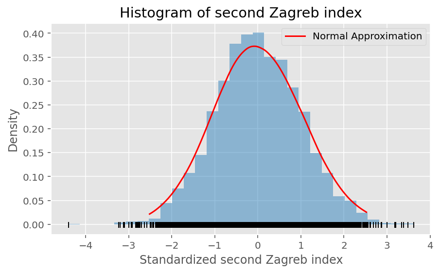
Figure 7: Histogram of the standardized second Zagreb index of $5,000$ independently generated random spiro chains with $n=10,000$; the thick red curve is the estimated density of the sample.

4 Concluding Remarks

In this paper, we propose a martingale approach to the study of topological indices in random spiro chains. The expected value, variance, exact distribution have been determined. Also, we formulate a martingale to characterize the asymptotic behavior of the topological indices. We show that the same analysis works here if we simply use a martingale central limit theorem instead of a classical central limit theorem. Moreover, we consider some particular topological indices, such as, Nirmala, Sombor, Randić and Zagreb index, in other words, we exploit the martingale approach.

References

- [\citeauthoryearDengDeng2012] Deng, H. (2012). Wiener indices of spiro and polyphenyl hexagonal chains. Mathematical and Computer Modelling 55(3-4), 634–644.
- [\citeauthoryearFang, You, and LiuFang et al.2021] Fang, X., L. You, and H. Liu (2021). The expected values of Sombor indices in random hexagonal chains, phenylene chains and Sombor indices of some chemical graphs. International Journal of Quantum Chemistry, e26740.
- [\citeauthoryearFeng and HuFeng and Hu2015] Feng, Q. and Z. Hu (2015). Asymptotic normality of the Zagreb index of random b-ary recursive trees. Dal’nevostochnyi Matematicheskii Zhurnal 15(1), 91–101.
- [\citeauthoryearGutmanGutman2021] Gutman, I. (2021). Geometric approach to degree-based topological indices: Sombor indices. MATCH Commun. Math. Comput. Chem.
- [\citeauthoryearGutman and KulliGutman and Kulli2021] Gutman, I. and V. Kulli (2021). Nirmala energy. Open Journal of Discrete Applied Mathematics 4(2), 11–16.
- [\citeauthoryearGutman, Kulli, and RedzepovicGutman et al.2021] Gutman, I., V. Kulli, and I. Redzepovic (2021). Nirmala index of Kragujevac trees. International Journal of Mathematics Trends and Technology 67(6), 44–49.
- [\citeauthoryearGutman and TrinajstićGutman and Trinajstić1972] Gutman, I. and N. Trinajstić (1972). Graph theory and molecular orbitals. Total -electron energy of alternant hydrocarbons. Chemical physics letters 17(4), 535–538.
- [\citeauthoryearHall and HeydeHall and Heyde2014] Hall, P. and C. C. Heyde (2014). Martingale limit theory and its application. New York: Academic press.
- [\citeauthoryearJahanbaniJahanbani2020] Jahanbani, A. (2020). The First Zagreb and Randić Indices in Random Spiro Chains. Polycyclic Aromatic Compounds, 1–9.
- [\citeauthoryearKazemiKazemi2021] Kazemi, R. (2021). Gordon-Scantlebury and Platt Indices of Random Plane-oriented Recursive Trees. Mathematics Interdisciplinary Research 6(1), 1–10.
- [\citeauthoryearKulliKulli2021] Kulli, V. (2021, 03). Nirmala Index. International Journal of Mathematics Trends and Technology 67, 8–12.
- [\citeauthoryearKulli, Chaluvaraju, and AshaKulli et al.2021] Kulli, V., B. Chaluvaraju, and T. Asha (2021). Computation of Nirmala indices of some chemical networks. Journal of Ultra Scientist of Physical Sciences-A 33(4), 30–41.
- [\citeauthoryearLi, Shi, and GaoLi et al.2021] Li, S., L. Shi, and W. Gao (2021). Topological indices computing on random chain structures. International Journal of Quantum Chemistry 121(8), e26589.
- [\citeauthoryearRandicRandic1975] Randic, M. (1975). Characterization of molecular branching. Journal of the American Chemical Society 97(23), 6609–6615.
- [\citeauthoryearRazaRaza2020] Raza, Z. (2020). The harmonic and second Zagreb indices in random polyphenyl and spiro chains. Polycyclic Aromatic Compounds, 1–10.
- [\citeauthoryearRazaRaza2021] Raza, Z. (2021). The expected values of some indices in random phenylene chains. The European Physical Journal Plus 136(1), 1–15.
- [\citeauthoryearRaza and ImranRaza and Imran2021] Raza, Z. and M. Imran (2021). Expected Values of Some Molecular Descriptors in Random Cyclooctane Chains. Symmetry 13(11), 2197.
- [\citeauthoryearSeverini et al.Severini et al.2012] Severini, T. A. et al. (2012). Elements of Distribution Theory. New York: Cambridge University Press.
- [\citeauthoryearWei, Ke, and HaoWei et al.2018] Wei, S., X. Ke, and G. Hao (2018). Comparing the excepted values of atom-bond connectivity and geometric–arithmetic indices in random spiro chains. Journal of inequalities and applications 2018(1), 1–11.
- [\citeauthoryearZhang, You, Liu, and HuangZhang et al.2021] Zhang, W., L. You, H. Liu, and Y. Huang (2021). The expected values and variances for sombor indices in a general random chain. Applied Mathematics and Computation 411, 126521.