Differentiable solver for time-dependent deformation problems with contact

Abstract.

We introduce a general differentiable solver for time-dependent deformation problems with contact and friction. Our approach uses a finite element discretization with a high-order time integrator coupled with the recently proposed incremental potential contact method for handling contact and friction forces to solve ODE- and PDE-constrained optimization problems on scenes with a complex geometry. It support static and dynamic problems and differentiation with respect to all physical parameters involved in the physical problem description, which include shape, material parameters, friction parameters, and initial conditions. Our analytically derived adjoint formulation is efficient, with a small overhead (typically less than 10% for nonlinear problems) over the forward simulation, and shares many similarities with the forward problem, allowing the reuse of large parts of existing forward simulator code.

We implement our approach on top of the open-source PolyFEM library, and demonstrate the applicability of our solver to shape design, initial condition optimization, and material estimation on both simulated results and in physical validations.

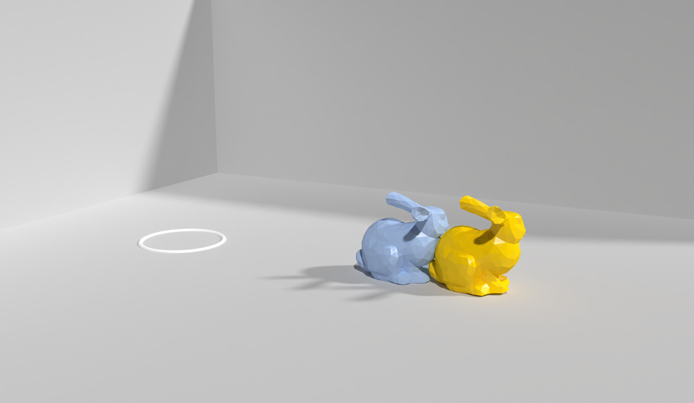
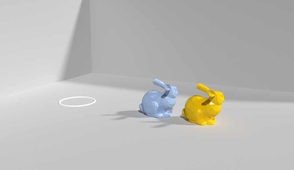
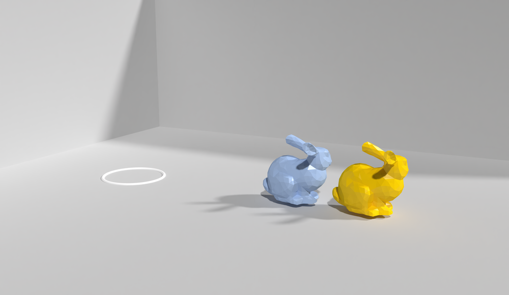
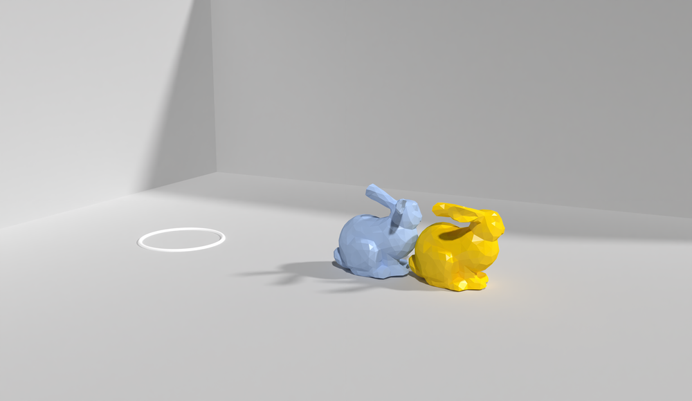
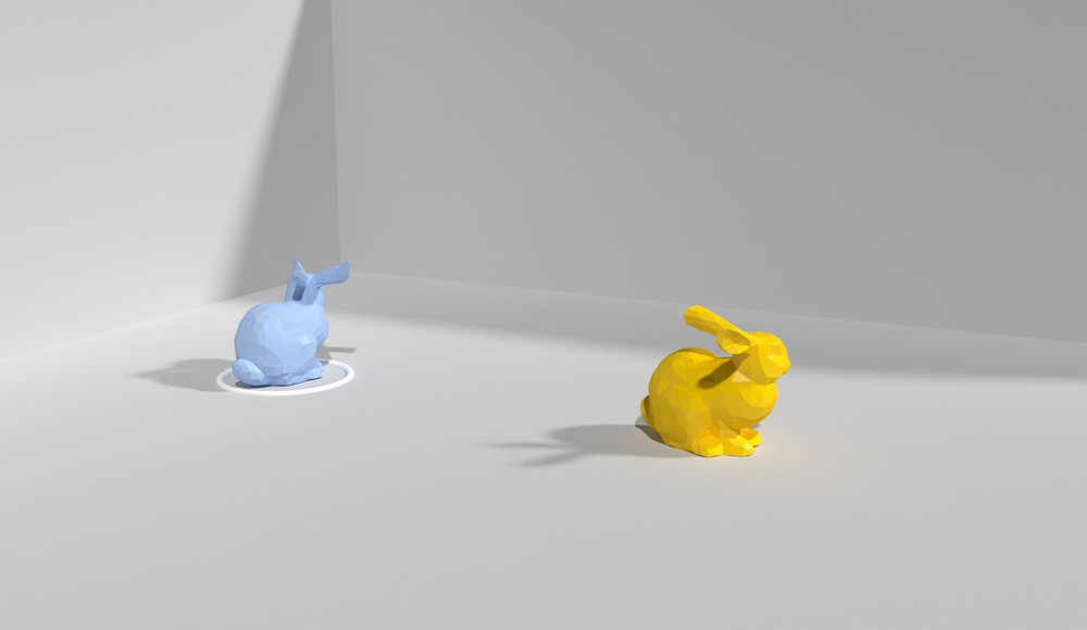
$t=0$

$t=0.15$

$t=1.5$

Figure 1. The direction and magnitude of the initial velocity of the yellow bunny is optimized to push, after contact, the blue bunny into the white circle marker. Top row is the initial configuration, and bottom row is our optimized result. This scene involves a elastodynamic simulation with a non-linear material model with contact and friction forces.

derivation explicitexpr

1. Introduction

ODE- and PDE-constrained optimization problems, i.e. the minimization of a functional depending on the state of a physical system modeled using a set of (partial) differential equations, appear in many application areas: optimized design in engineering and architecture, metamaterial design in material science, inverse problems in biomedical applications, controllable physically-based modeling in computer graphics, control policy optimization, and physical parameter estimation in robotics.

A common family of PDE-constrained optimization problems in graphics, robotics, and engineering involve static or time-dependent elastic deforming objects interacting with each other via contact and friction forces. A significant number of approaches have been proposed to tackle PDE-constrained optimization problems of this type (Section 2).

However, these approaches often make application-specific assumptions aimed at simplifying the differentiable simulator, often sacrificing generality (e.g., handling contact only with simple rigid obstacles or differentiating with respect to material parameters only), robustness (e.g., using a contact model that requires per-scene parameter tuning to prevent failure), accuracy (e.g., using inaccurate spatial discretizations, non-physical material, or friction models), or scalability (e.g., restricting the number of system parameters with respect to which it can be optimized).

Building on and integrating a broad range of previous work on PDE-constrained optimization, including shape optimization, material property estimation, and trajectory control, we develop a differentiable solver that eliminates or reduces all of these shortcomings. Our solver has the following characteristics:

1. To increase generality, we support differentiation with respect to all physical parameters involved in the physical problem description: shape, material parameters, friction parameters, and initial conditions. An arbitrary subset of these parameters can be used in the objective functions.

2. Our contact/friction formulation builds upon the recently proposed Incremental Potential Contact approach (Li et al., 2020). Our differentiable simulator supports complex geometry, is automatic and robust (with only two main parameters controlling the accuracy of the spatial and temporal discretizations), and guarantees physically valid configurations at all timesteps, without intersections nor inverted elements.

3. We use a standard finite element discretization of arbitrary order, both in space and time with non-linear elasticity material models, ensuring accuracy.

4. Our formulation supports both static and dynamic problems.

5. Our differentiation approach is efficient. The computation of the derivatives for one PDE-constrained optimization step is at most as expensive as a forward evaluation of the underlying forward simulation of the physical systems, and for nonlinear problems we observe that the differentiability adds at most 10% to the cost.

The foundation of our approach, similar to a number of previous works, is the adjoint method, which we systematically apply to obtain derivatives with respect to all parameters in a unified way, and computing force- and objective-specific derivatives, whenever possible, in a general form, simplifying addition of new forces and objectives to the system. While, compared to alternative approaches, this method requires more derivations, it has significant advantages: compared to finite differences, it supports a large number of system parameters without a major impact on performance; compared to automatic differentiation, it allows the reuse of (non-differentiable) solver code extensively, as the adjoint equations solved to obtain gradients are similar to the original physics equations.

The technical contributions of our work support the central goal of developing a comprehensive and extensible unified framework for differentiable deformable object simulation. Most importantly, these include:

• Our space-domain adjoint derivation is done in terms of solution and material parameter approximations in a continuous finite-element basis, as opposed to purely discrete form. This makes the derivation of explicit expressions shape derivatives practical, and critical for accurate shape derivatives and large deformations. In comparison, methods such as (Hahn et al., 2019) construct the discrete system first and then treat it as an algebraic system. At the same time, we maintain consistency, i.e., the gradients we compute are exactly equal to the ones obtained for the discretized system by direct differentiation.

• We introduce a differentiable version of IPC for contact and friction which ensures robust handling of general contact. While support for contact and friction has been considered in previous differentiable simulators, it has always been considered in special cases such as: restricting to planes, ignoring self-collision, or using Mortar methods requiring manual specification of collision pairs (Section 2). In contrast, our formulation inherits the robustness and generality of IPC, it supports contacts between general triangular meshes, handles self-collision, and does not require collision pairs to be specified.

We demonstrate the effectiveness of our approach on a set of examples involving multiple objectives and optimizing for the shape, material parameters, friction parameters, and initial conditions.

2. Related Work

We summarize the most relevant simulation frameworks, primarily focusing on those supporting differentiable simulation of elastic deformable objects and robotics systems.

For the works that are closer to our targeted applications, we provide an explicit breakdown of which subset of the characteristics of our solver they support (Table 1). We also highlight the generality of our solver by explicitly identifying which solvers cannot reproduce the examples in our paper due to unsupported features (Table 2). These two tables demonstrate the benefits of our formulation and the wide applicability of our solvers, which we will release as an open-source project to foster its adoption.

Table 1. The table columns correspond to five main comparison characteristics: (1) High-order space and time discretization, (2) supported optimization parameters (3) support for complex contacts between arbitrary surfaces, including self-collision, (4) support for static and dynamic simulations, and (5) method for the derivatives computation. No existing differentiable solver supports all features of our solver at the same time, and in particular, most do not support differentiating with respect to the shape of the domain.

Method	(1) HO	(2) Parameters	(3) Collisions	(4) Static and Dynamic	(5) Differentiation
Elastic Texture (Panetta et al., 2015)	Yes	Shape	No support	Static-Only	Adjoint
CB-Assemblies (Tozoni et al., 2021)	Yes	Shape	Static and Prescribed	Static-Only	Adjoint
ADD (Geilinger et al., 2020)	No	Material, Initial	Only planes or SDF, no self-collisions	Dynamic-Only	Adjoint
GradSim (Jatavallabhula et al., 2021)	No	Material, Initial	Only planes, no self-collisions	Dynamic-Only	Code transformation
DiSECt (Heiden et al., 2021)	No	Material	Only planes or SDF, no friction	Dynamic-Only	Code transformation/autodiff
NeuralSim (Heiden et al., 2020)	No	Material, Initial	Only rigid-bodies	Dynamic-Only	Code transformation/autodiff
DiffPD (Du et al., 2021)	No	Material, Initial	Only planes or SDF	Dynamic-Only	Adjoint
Ours	Yes	Shape, Material, Initial	No restrictions	Static and Dynamic	Adjoint

Table 2. To showcase the differences between our approach and other differentiable simulators, we show which simulators support the features needed for each experiment in our paper. We refer to the figure captions for more details on each experiment but highlight that most existing simulators do not support shape optimization (Fig5–13) and the ones that do lack support for dynamic.
From left to right: Fig1 and 22 require contact handling between soft bodies; Fig5–13 require shape optimization; Fig16–17 require material distribution optimization; and Fig19 and 21 require self-collision handling.

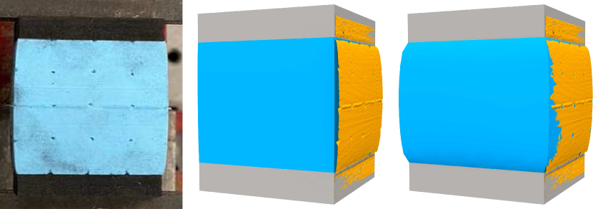
Physical Experiment Setup.

Initial shape.

Optimized.

Figure 18. Static: Cube. Material optimization (blue) to match real data (orange).

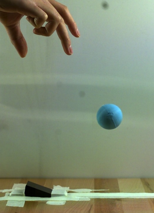
Physical experiment.

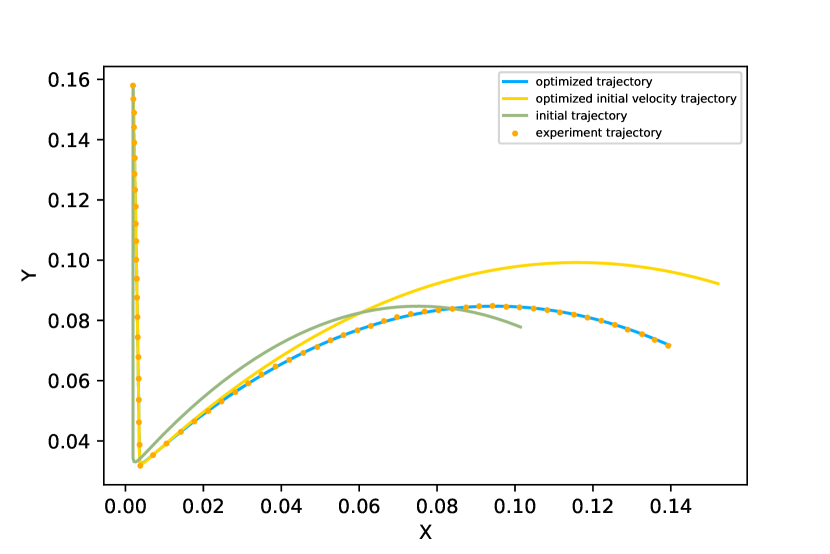
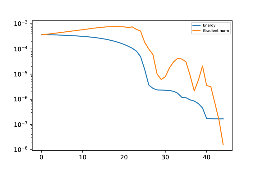
$xy$ coordinates of the barycenter of the ball over time. Energy and gradient over the optimization iterations.

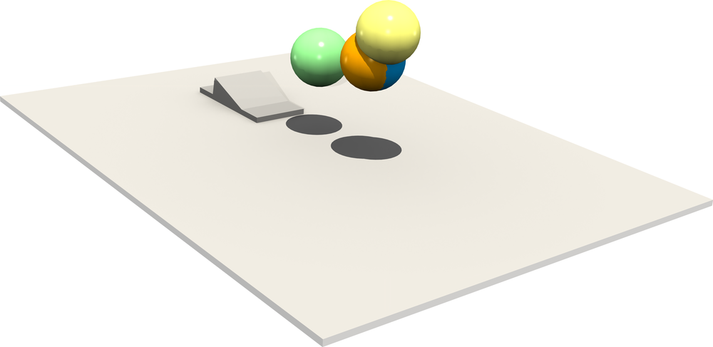
Initial guess (green), initial velocity optimization (yellow), material optimization (blue), and experimental data (orange).

Figure 23. Transient: Physical Experiment Bouncing Ball. Optimize the material and initial velocity of the ball to match the observed physical result.

Method	Fig1	Fig5–10	Fig11–13	Fig14	Fig16–17	Fig18	Fig19	Fig20	Fig21	Fig22	Fig23
Elastic Texture (Panetta et al., 2015)					Y
CB-Assemblies (Tozoni et al., 2021)		Y
ADD (Geilinger et al., 2020)				Y		Y		Y			Y
GradSim (Jatavallabhula et al., 2021)				Y		Y		Y			Y
DiSECt (Heiden et al., 2021)						Y		Y			Y
NeuralSim (Heiden et al., 2020)
DiffPD (Du et al., 2021)				Y		Y		Y	Y		Y
Ours	Y	Y	Y	Y	Y	Y	Y	Y	Y	Y	Y

Differentiable deformable object simulators

Numerous differentiable elastic body simulators have been developed for applications in optimal design of shapes (Panetta et al., 2015, 2017; Tozoni et al., 2020; Ly et al., 2018), actuators (Skouras et al., 2013; Chen et al., 2020; Maloisel et al., 2021), sensors (Tapia et al., 2020), material characterization (Hahn et al., 2019; Schumacher et al., 2020), and robotic control (Bern et al., 2019; Hoshyari et al., 2019). These simulators broadly fit into three categories: (i) those employing analytic derivatives computed using sensitivity analysis; (ii) those using automatic differentiation libraries (Hu et al., 2019a; Heiden et al., 2020) based on overloading, or algorithmic differentiation (iii) neural surrogate models replacing the entire simulation with a differentiable neural network (Chang et al., 2016; Zhang et al., 2016; Baque et al., 2018; Bern et al., 2020).

Our method belongs to the first category: analytic sensitivity analysis generally requires manual differentiation of the physics equations, but allows one to reuse existing solvers most easily; direct differentiation is feasible only if the number of parameters is very small; large number of parameters requires construction of the adjoint equations for specific functionals (Liang et al., 2019; Qiao et al., 2020; Bern et al., 2019; Rojas et al., 2021; Du et al., 2021; Li et al., 2022; Ly et al., 2018), and is more efficient than all other approaches. One exception is Dolphin-Adjoint (Mitusch et al., 2019), which automatically and robustly derives adjoint models for models written in the finite element software FEniCS (Alnaes et al., 2015). Automatic differentiation methods are most general but require existing simulators to be rewritten using data-structures required for gradients and Hessians, and typically incurs a significant performance penalty. Surrogate models, though promising dramatic speedups, require huge training sets for even simple design spaces (Gavriil et al., 2020), and currently are unsuitable for high-precision applications (Bächer et al., 2021). Code transformation and auto-differentiation, e.g. in simulators such as (Jatavallabhula et al., 2021) and (Heiden et al., 2021), based on technology developed in NVIDIA Warp (Xu et al., 2022), while potentially allowing one to reuse existing codes, typically places a few limitations on what the code may contain. To the best of our knowledge, none of the existing simulators support robust handling of contact and friction for complex geometries, and they only support a subset of the design parameters compared to the more general formulation of this paper.

We provide direct comparisons of our solver, (Du et al., 2021), and (Jatavallabhula et al., 2021) in Section 9.5.

Differentiable Simulations with Contact

Differentiable simulators incorporating various contact models have recently been developed for rigid (Heiden et al., 2020) and soft bodies (Liang et al., 2019; Qiao et al., 2020; Geilinger et al., 2020; Jatavallabhula et al., 2021; Heiden et al., 2021). These contact models often require per-scene parameter tuning if complex contact scenarios are present, which makes these methods hard to use in optimization, especially shape optimization.

Our approach uses the recently proposed Incremental Potential Contact (IPC) formulation (Li et al., 2020), replacing the traditional zero-gap assumption (Wriggers, 1995; Kikuchi and Oden, 1988; Stewart, 2001; Brogliato, 1999; Belytschko et al., 2000; Bridson et al., 2002; Otaduy et al., 2009; Harmon et al., 2008, 2009; Daviet et al., 2011; Verschoor and Jalba, 2019) with a smooth version ensuring a (small) non-zero separation between objects at every frame of the simulation. This approach was designed with the explicit goal of guaranteeing robustness and its smooth formulations of contact and friction avoids the need for handling non-smooth constraints.

Stupkiewicz et al. (2010) are one of the few who demonstrate sensitivity analysis of elastic problems with contact with respect to a range of parameters, including shape and material properties. This method, tested on a limited set of regular-grid problems, uses direct differentiation requiring a solve per parameter, and does not use a robust contact model.

We compare our solver, (Du et al., 2021), and (Jatavallabhula et al., 2021) in Section 9.5 in scenes involving both contact and self-contact.

Shape and topology optimization with contact

Historically shape optimization was primarily considered separately, e.g., for physical parameter or initial condition estimation, primarily in static settings, often with additional assumptions on bodies involved in contact.

Some previous works in this area have considered the specific case of optimization in the presence of contact between a soft body with fixed rigid surfaces (Beremlijski et al., 2014; Haslinger et al., 1986; Herskovits et al., 2000). Other works, like ours, have studied the interaction of two or more deformable bodies in contact (Desmorat, 2007; Stupkiewicz et al., 2010; Maury et al., 2017; Tozoni et al., 2021). Most papers do not consider friction or use a simplified model (compared to the standard Coulomb formulation) as discussed by Maury et al. (2017).

Most closely related to our approach, Maury et al. (2017) presented a level set discretization technique where contact and friction were modeled with penalty terms, using smooth approximations to the problem. Using a similar contact and friction model, Tozoni et al. (2021) designed a shape optimization technique that focused on reducing stress of static assemblies that are held together by contact and friction. Both these works followed the mathematical model of contact presented by Eck et al. (2005), which allows for interpenetration and assumed that contact zones are fixed.

Our approach supports dynamic simulation, allows contact zones to change with both optimization parameter changes and in the course of the simulation, and supports contact and self-contact between arbitrary deformable objects.

Another closely related work Hsu et al. (2022) presented a general technique to optimize the rest shape and initial displacement of input geometries, so that the structures are stable purely because of frictional contact. Note that IPC is also used in the forward simulation in this paper, but not for optimization.

Table 3. Notation.

Domains and bases
$D_{d}$	Domain dimension, $2$ or $3$.
$D_{s}$	Solution dimension, $1$, $2$ or $3$.
$\Omega_{\mathrm{ref}}$	Reference domain $\Omega_{\mathrm{ref}}\subset\mathbb{R}^{D_{d}}$ consists of copies of identical reference elements $\hat{K}_{j}$, $j=1\ldots n_{K}$ identified along edges.
$\hat{x}_{\ell}$ and $\hat{z}_{\ell}$	Nodes are points in $\Omega_{\mathrm{ref}}$ used to define bases, $\ell=1\ldots n^{x}_{N}$, and $1\ldots n^{z}_{N}$ respectively. The set of nodes $\hat{z}_{\ell}$ does not include nodes with Dirichlet boundary conditions; the set of nodes $x_{i}$ does include these nodes.
$\hat{\phi}^{\ell}$ and $\hat{\xi}^{\ell}$	FE basis functions are scalar basis functions defined on $\Omega_{\mathrm{ref}}$; $\hat{\xi}^{\ell}$ correspond to nodes $\hat{x}_{i}$, and is used for geometric maps (we use p.w. linear basis); $\hat{\phi}^{\ell}$ correspond to $\hat{z}_{\ell}$ and used for all other quantities (arbitrary order Lagrangian).
${\bar{q}}$, ${\bar{q}}^{j}(y^{j})$, ${\mathbf{{\bar{q}}}}$, $x_{\ell}$	Geometric map ${\bar{q}}$ embedding a reference element in space, is defined on each $\hat{K}_{j}$ in $\Omega_{\mathrm{ref}}$ with local coordinates $y^{j}$ as ${\bar{q}}^{j}(y^{j})=\sum_{\ell}x_{\ell}\hat{\xi}^{\ell}(y^{j}),$ where $x_{\ell}\in\mathbb{R}^{D_{d}}$ are the positions of the nodes of the element $j$ forming the vector ${\mathbf{{\bar{q}}}}$. Concatenation of these maps yields the global geometric map ${\bar{q}}:\Omega_{\mathrm{ref}}\rightarrow\mathbb{R}^{D_{d}}$.
$\Omega_{\mathbf{{\bar{q}}}}$	Physical domain is the domain on which the PDE is solved, parametrized by ${\mathbf{{\bar{q}}}}$, $\Omega_{\mathbf{{\bar{q}}}}={\bar{q}}(\Omega_{\mathrm{ref}})$. The global coordinate on $\Omega_{\mathbf{{\bar{q}}}}$ is $x=x^{\mathbf{{\bar{q}}}}\in\mathbb{R}^{D_{d}}$.
$\phi^{\ell}(x)$,$\xi^{\ell}(x)$	FE bases on $\Omega_{\mathbf{{\bar{q}}}}$. The bases $\hat{\phi}^{\ell}$ and $\hat{\xi}^{\ell}$ can be pushed forward to the domain $\Omega_{\mathbf{{\bar{q}}}}$ via $\phi(x)=\hat{\phi}\circ{\bar{q}}^{-1}(x)$ and $\xi(x)=\hat{\xi}\circ{\bar{q}}^{-1}(x)$.
$\Omega_{{\mathbf{{\bar{q}}}}+\bm{\theta}t}$	Perturbed domain obtained using a perturbation direction $\bm{\theta}$ in ${\mathbf{{\bar{q}}}}$. Perturbation $\theta(x)\in\mathbb{R}^{D_{d}}$ is: $\theta=\theta(x)=\sum_{\ell}\theta_{\ell}\,\hat{\xi}^{\ell}\circ({\bar{q}}^{j})^{-1}(x)=\sum_{\ell}\theta_{\ell}\,\xi^{\ell}(x)$.

Functions on physical domain $\Omega_{\mathbf{{\bar{q}}}}$
$u_{\mathbf{{\bar{q}}}}(x)$,$\mathbf{u}$	PDE solution defined on $\Omega_{\mathbf{{\bar{q}}}}$ with values in $\mathbb{R}^{D_{s}}$. We denote the vector of coefficients of $u$ in the FE basis $\phi$ by $\mathbf{u}$. $u(x)=\sum_{\ell}u_{\ell}\hat{\phi}^{\ell}\circ{\bar{q}}^{-1}(x)=\sum_{\ell}u_{\ell}\phi^{\ell}(x).$
$w(x)$, $\psi(x)$,$\mathbf{w}$,$\bm{\psi}$	Test functions (scalar) defined similarly to $u(x)$ in the same basis and vectors of their coefficients are $\mathbf{w}$ and $\bm{\psi}$.
$p(x)$,$\mathbf{p}$	Adjoint solution is the solution of the adjoint equation and the vector of its coefficients, with values in $\mathbb{R}^{D_{s}}$.
$q^{m}(x)$, $\mathbf{q}^{m}$	$m$-th optimization parameter $q^{m}(x)=\sum_{\ell=1}^{n^{m}_{q}}q^{m}_{\ell}\zeta^{\ell}(x)$ with a basis $\zeta^{\ell}$ with values in $\mathbb{R}^{D^{m}_{q}}$ parameters can be material properties, boundary conditions etc, defined on all or parts of $\Omega_{\bar{q}}$. For the geometry map ${\bar{q}}$, $\xi$ on $\mathrm{Dom}({\bar{q}})=\Omega_{\mathrm{ref}}$, and $\zeta^{\ell}=\xi^{\ell}$.
PDE and derivatives
$\mathbf{h}(\mathbf{u},\mathbf{q})=0$	Discretized form of the PDE, i.e., a system of $n_{u}$ algebraic equations with components of $\mathbf{u}$ as unknowns.
$J(\mathbf{u},\mathbf{q})$	Discretized form of the objective.
$\partial_{\mathbf{q}}a(\mathbf{u},\mathbf{q})$	Derivative of a (possibly) vector quantity $a$ with respect to a vector of optimization parameters, not including dependence through $u$. The vector is the vector of coefficients of one of $q^{m}$ or ${\bar{q}}$. If the dimension of $a$ is $n_{a}$, then $\partial_{\mathbf{q}}\mathbf{a}$ is a matrix of size $n_{a}\times D^{m}_{q}n^{m}_{q}$.
$\partial_{\mathbf{u}}a(\mathbf{u},\mathbf{q})$	Derivative of a quantity $a$ with respect to the the PDE solution $u$; it is a vector of length $D_{s}n_{u}$.
$d_{\mathbf{q}}a(\mathbf{u},\mathbf{q})$	Full derivative of $a$ with respect to $\mathbf{q}$, including through the dependence on $u$.
$\nabla a(v)$, $\nabla_{i}a(v,w)$	Derivatives of $a$ with respect to arguments $v,w\in\mathbb{R}^{D}$.

Meshfree methods

A number of differentiable simulation methods use meshfree discretizations. Especially for shape optimization, methods like XFEM (Schumacher et al., 2018; Hafner et al., 2019) and MPM (Hu et al., 2019b) that do not maintain conforming meshes are often considered to circumvent remeshing-induced discontinuities (Bächer et al., 2021). However, these methods sacrifice accuracy (de Vaucorbeil et al., 2019), particularly for stress minimization problems (Sharma and Maute, 2018). Our approach computes accurate displacement and stressed by using a finite element method framework using high-order elements, coupled with dynamic remeshing to compensate for the distortion introduced by large deformations.

3. Overview

In Sections 4-8, we provide a self-contained description of our method. While this contains a mix of known and new material, we aim to present all components of the method in a unified and systematic notation to ensure reproduciblity.

Typographical conventions

We use lower-case italic for functions $a(z)$ and variables $z$, with both $z$ and $a$ in $\mathbb{R}^{D}$, where $D=2,3$. Boldface lower-case letters ($\mathbf{a}$) are used for vectors of coefficients of a FEM (or any other) discretization of a function. For a vector or matrix quantity, superscripts are used to index whole vectors or matrices: e.g., $\mathbf{p}^{i}$ may denote $\mathbf{p}$ at time step $i$. Subscripts are used for the indices of components of a vector, e.g., $a(z)=\sum_{\ell=1}^{n}a_{\ell}\phi^{\ell}(z)$ means that the function $a(z):\mathbb{R}\rightarrow\mathbb{R}^{D}$ is a linear combination of basis functions $\phi^{\ell}$, with coefficients $a_{\ell}$ which are components of $\mathbf{a}$. If $a(z)$ has values in $\mathbb{R}^{D}$, its coefficients in a scalar basis $\phi^{\ell}$ are $D$-dimensional, Then $\mathbf{a}$ is a vector of length $D\cdot n$, with $D$ coordinates of each component of $a_{\ell}$ in sequential entries.

General problem form

We solve static and dynamic optimization problems of the form

(1) $$\min_{q}J(u,x,q),\;\mbox{such that, $\mathcal{H}(u,x,q)=0$}$$

and

(2) $$\small\begin{split}&\hskip 50.0pt\min_{q}J(\mathbf{u},\mathbf{q})=\min_{q}\int_{t=0}^{T}J(\mathbf{u},t,\mathbf{q})\;\\ &\mbox{such that $\rho\ddot{u}=\mathcal{H}(u,x,t,q)$ on $\Omega_{\mathbf{{\bar{q}}}}$},\;u(0)=g^{u}(q),\dot{u}(0)=g^{v}(q),\end{split}$$

where $J$ is an objective, possibly including constraints in penalty form, $u(x,t)$ is the displacement of a material point $x$ satisfying a static or dynamic physics equation, and $g^{u}$ and $g^{v}$ are the initial conditions for the displacements and velocities. In this work, we consider nonlinear elastic deformation, contact, friction, and damping forces. We assume the density $\rho$ to be constant in time. The optimization parameter functions $q=({\mathbf{{\bar{q}}}},\mathbf{q}^{1},\ldots,\mathbf{q}^{m})$ include all parameters of the system: material properties (elastic, friction, and damping), object shape, and initial and boundary conditions. The first of these, ${\bar{q}}$ plays a special role: it determines the shape of the domain $\Omega_{\mathbf{{\bar{q}}}}$ on which the PDE is defined; it is a function on a reference domain $\Omega_{\mathrm{ref}}$ defining its deformation. Parameters $q^{i}$ may be global constants, or dependent on the points of the reference domain, or pairs of points (as it is the case for the friction coefficient).

This problem statement is similar to (Geilinger et al., 2020) and other works on differentiable simulators; however, our goal is to support full differentiability, including shape, in a systematic way (see Table 1 for details) which affects the adjoint formulation and requires deriving expressions for a number of gradients of forces and functionals.

Discrete problem

We postpone the exact description of the discrete problem to Section 5. The discretized static problem obtained using FEM discretization has the general form:

(3) $$\min_{\mathbf{q}}J(\mathbf{u},\mathbf{q}),\;\mbox{s.t., $\mathbf{h}(\mathbf{u},\mathbf{q})=0$},$$

where $\mathbf{u}$ is the vector of FE basis coefficients of $u$ and $\mathbf{q}$ is the concatenation of the vectors of coefficients of ${\mathbf{{\bar{q}}}},\mathbf{q}^{1},\ldots,\mathbf{q}^{m}$.

The dynamic discretized problem with BDF of order $m$ discretization in time has the general form:

(4) $$\begin{split}&\min_{\mathbf{q}}J(\mathbf{u},\mathbf{q})=\min_{\mathbf{q}}\sum_{i=0}^{N}w_{i}J_{i}(\mathbf{u}^{i},\mathbf{q})\\ &\mathbf{u}^{i}+\sum_{j=1}^{\min(i,m)}\alpha^{i}_{j}\mathbf{u}^{i-j}=\beta_{i}\Delta t\,\mathbf{v}^{i}\\ &M\bigg{(}\mathbf{v}^{i}+\sum_{j=1}^{\min(i,m)}\alpha^{i}_{j}\mathbf{v}^{i-j}\bigg{)}=\beta_{i}\Delta t\,\mathbf{h}^{i}(\mathbf{u}^{i},\mathbf{u}^{i-1},\mathbf{q})=\hat{\mathbf{h}}^{i},\end{split}$$

where $M$ is the mass matrix. The higher-order BDF schemes need to be initialized with lower-order steps; more specifically, $\alpha^{i}_{j}$ is $j$-th coefficient of BDF$i$, for $1\leqslant i<m$, and $j$-th coefficient of BDF$m$ otherwise. In the formulation above, $\mathbf{h}(\mathbf{u},\mathbf{q})$ does not depend on velocities $\mathbf{v}$. If the dependence on velocities is needed, as for damping forces, we discretize in time, and handle it as dependence on $\mathbf{u}$ at different time steps.

Overview of the method

We aim to present a complete, largely self-contained formulation, to ensure reproducibility as well as support easy addition of new types of forces. This requires restating briefly some of the known facts and formulas using our notation; we identify parts that are not present in previous work.

We first assume the discretized form of the problem (3) and (4), and derive consistent adjoint equations for the static and dynamic cases.

Each force and objective can be added to this general framework by deriving a set of matrices and vectors needed to compute partial force and objective derivatives.

We then proceed by computing these quantities analytically for the set of forces involved in our formulation, and a broad selection of functionals, including most used in the previous work both on differentiable dynamic simulation and shape optimization. We compute these in a form that allows for easy remeshing of $\Omega_{\mathrm{ref}}$ and $\Omega_{\mathbf{{\bar{q}}}}$, which is necessary for the large changes in physical domain introduced by shape optimization.

4. Adjoint-based objective derivatives

4.1. Static case

The derivatives of the objective $J$ with respect to optimization parameters can be computed efficiently using the classic adjoint method. While the basic principles of the derivation are well-known, we summarize it in the context of our problem. The general form of our equations is similar to (Geilinger et al., 2020), which in turn is based on (Hahn et al., 2019). We derive the abstract form of the adjoint system for a general form of BDF time stepping, and importantly we ensure that the dynamic adjoint solution is consistent, i.e., yields identical, rather than approximately identical, results to direct differentiation, as well as consider variable mass matrix needed for shape derivatives.

With the adjoint method, the gradient with respect to any number of parameters can be obtained by solving a single additional linear PDE (the adjoint PDE), and then evaluating an expression depending on this unknown. The adjoint PDE is obtained by considering the Lagrangian

(5) $$\mathcal{L} =J(\mathbf{u},\mathbf{q})$$ {objective term}

(6) $$+\mathbf{p}^{T}\,\mathbf{h}(\mathbf{u},\mathbf{q})$$ {physical constraint term}

and differentiating it with respect to the parameters $\mathbf{q}$:

(7) $$d_{\mathbf{q}}\mathcal{L} =\partial_{\mathbf{q}}J+\partial_{\mathbf{u}}J\,d_{\mathbf{q}}\mathbf{u}+\mathbf{p}^{T}\,\partial_{\mathbf{q}}\mathbf{h}\ +\mathbf{p}^{T}\,\partial_{\mathbf{u}}\mathbf{h}\,d_{\mathbf{q}}\mathbf{u}.$$

$d_{\mathbf{q}}\mathcal{L}\,$ is expensive to compute if the dimension of $\mathbf{q}$ is large; a direct computation involves computing $d_{q_{m}}\mathbf{u}$ (how solution changes according to parameter $q_{m}$) for every optimized parameter $q_{m}$ in $\mathbf{q}$, which means solving $\lvert q\rvert$ different linear PDEs. Isolating all terms multiplying $d_{\mathbf{q}}\mathbf{u}$:

(8) $$d_{\mathbf{q}}\mathcal{L} =\partial_{\mathbf{q}}J+\mathbf{p}^{T}\,\partial_{\mathbf{q}}\mathbf{h}+\mathopen{}\mathclose{{}\left(\partial_{\mathbf{u}}J+\mathbf{p}^{T}\,\partial_{\mathbf{u}}\mathbf{h}}\right)\,d_{\mathbf{q}}\mathbf{u}.$$

We can then eliminate the last term by choosing the adjoint variable $\mathbf{p}$ such that it solves the adjoint problem:

(9) $$\mathbf{p}^{T}\,\partial_{\mathbf{u}}\mathbf{h}=-\partial_{\mathbf{u}}J.$$

Then, by plugging the solution $\mathbf{p}$ of the adjoint PDE into the Lagrangian, we obtain the final shape derivative:

(10) $$d_{\mathbf{q}}J=d_{\mathbf{q}}\mathcal{L}(\mathbf{p}) =\partial_{\mathbf{q}}J+\mathbf{p}^{T}\,\partial_{\mathbf{q}}\mathbf{h}.$$

Combining contributions from different forces and objectives together

Our discretized equation has the form

$$\mathbf{h}(\mathbf{u},\mathbf{q})=\sum_{k}\mathbf{h}^{k}(\mathbf{u},\mathbf{q})=0,$$

where $\mathbf{h}^{k}$ is a contribution from each type of force (elasticity forces, contact forces, etc). Similarly, the objective $J$ is a sum of contributions from several objective components or constraints in penalty form:

$$J(\mathbf{u},\mathbf{q})=\sum_{\ell}J^{\ell}(\mathbf{u},\mathbf{q}).$$

Thus, the adjoint system and the full parametric derivative have the following form, respectively:

(11) $$\begin{split}\mathbf{p}^{T}\mathopen{}\mathclose{{}\left(\sum_{k}\partial_{\mathbf{u}}\mathbf{h}^{k}}\right)&=-\sum_{\ell}\partial_{\mathbf{u}}J^{\ell},\\ d_{\mathbf{q}}J&=\sum_{\ell}\partial_{\mathbf{q}}J^{\ell}+\sum_{k}\mathbf{p}^{T}\partial_{\mathbf{q}}\mathbf{h}^{k}.\end{split}$$

Thus, for each force, we need $\partial_{\mathbf{u}}\mathbf{h}^{k}$ and $\partial_{\mathbf{q}}\mathbf{h}^{k}$ and each objective component, $\partial_{\mathbf{u}}J^{k}$ and $\partial_{\mathbf{q}}J^{\ell}$.

4.2. Dynamic case

Discrete time-dependent Lagrangian

We write the time-dependent Lagrangian $\mathcal{L}$ for the functional $J$ viewing the equations for $\dot{\mathbf{v}}$ and $\dot{\mathbf{u}}$ as constraints with Lagrange multipliers $\mathbf{p}$ and $\bm{\mu}$.

Similar to the static case, we expand the derivative $d_{\mathbf{q}}\mathcal{L}$, and isolate the terms containing $d_{\mathbf{q}}\mathbf{u}$ and $d_{\mathbf{q}}\mathbf{v}$. By setting the sum of each of these two sets of terms to zero, we obtain two adjoint equations.

Our Lagrangian consists of three parts, corresponding to the objective ($J$), physics constraints ($\mathcal{L}_{c}$), and initial condition constraints ($\mathcal{L}_{in}$):

$$\mathcal{L}(\mathbf{u},\mathbf{v},\mathbf{p},\bm{\mu},\mathbf{q})=J(\mathbf{u},\mathbf{q})+\mathcal{L}_{c}(\mathbf{u},\mathbf{v},\mathbf{p},\bm{\mu},\mathbf{q})+\mathcal{L}_{in}(\mathbf{u}^{0},\mathbf{v}^{0},\mathbf{p}^{0},\bm{\mu}^{0},\mathbf{q}),$$

where

$$\mathcal{L}_{in}=\mathbf{p}_{0}^{T}(\mathbf{v}^{0}-\mathbf{g}^{v})+\bm{\mu}_{0}^{T}(\mathbf{u}^{0}-\mathbf{g}^{u}),$$

and

$$\small\mathcal{L}_{c}=\sum_{i=1}^{N}\mathbf{p}^{T}_{i}M\bigg{(}\mathbf{v}^{i}+\sum_{j=1}^{\min(i,m)}\alpha^{i}_{j}\mathbf{v}^{i-j}-\hat{\mathbf{h}}^{i}\bigg{)}+\bm{\mu}^{T}_{i}\bigg{(}\mathbf{u}^{i}+\sum_{j=1}^{\min(i,m)}\alpha^{i}_{j}\mathbf{u}^{i-j}-\beta_{i}\Delta t\,\mathbf{v}^{i}\bigg{)}.$$

Adjoint equations

As shown in the Appendix, this leads to the following adjoint equations:

(12) $$\bigg{(}\mathbf{p}_{i}+\sum_{j=1}^{\min(m,N-i)}\alpha^{i+j}_{j}\mathbf{p}_{i+j}\bigg{)}=\beta_{i}\Delta t\,\bm{\nu}_{i}$$

$$M^{T}\mathopen{}\mathclose{{}\left(\bm{\nu}_{i}+\sum_{j=1}^{\min(m,N-i)}\alpha^{i+j}_{j}\bm{\nu}_{i+j}}\right)=$$

$$(\partial_{\mathbf{u}^{i}}\hat{\mathbf{h}}^{i})^{T}\mathbf{p}_{i}+(\partial_{\mathbf{u}^{i}}\hat{\mathbf{h}}^{i+1})^{T}\mathbf{p}_{i+1}-(\partial_{\mathbf{u}}\hat{J}^{i})^{T},$$

where we introduce a new variable $\bm{\nu}$ satisfying $\bm{\mu}=M^{T}\bm{\nu}$.

Note that this system is very similar to the forward time-stepping, with the following differences: it proceeds backwards, from $\bm{\nu}_{i+1}$ to $\bm{\nu}_{i}$; there is a single linear solve per time step, rather than a nonlinear solve as for the forward system; for higher-order time stepping the first few steps in the forward system are lower-order BDF steps; however, this is not the case for the adjoint system: to maintain consistency, we derive the initial low-order steps from the forward system.

By introducing $\mathbf{p}_{N+1},\ \bm{\nu}_{N+1}$, the initial condition can be simplified as

(13) $$\mathbf{p}_{N+1}=0,$$

$$\bm{\nu}_{N+1}=0.$$

The first (last in the adjoint solve) values need to be treated separately, as shown in Appendix A.2:

(14) $$\bm{\mu}_{0}=-(\partial_{\mathbf{u}}\hat{J}^{0})^{T}-\sum_{j=1}^{m}\alpha^{j}_{j}\bm{\mu}_{j}+\mathbf{p}_{1}^{T}\partial_{\mathbf{u}^{0}}\hat{\mathbf{h}}^{1},\;\mathbf{p}_{0}=-\sum_{j=1}^{m}\alpha^{j}_{j}M^{T}\mathbf{p}_{j}.$$

Computing the derivative of $J$ from the forward and adjoint solutions

From the adjoint variables, we can compute $d_{\mathbf{q}}J=d_{\mathbf{q}}\mathcal{L}$:

(15) $$d_{\mathbf{q}}J =-\mathbf{p}_{0}^{T}\partial_{\mathbf{q}}\mathbf{g}^{v}-\bm{\mu}_{0}^{T}\partial_{\mathbf{q}}\mathbf{g}^{u}$$

$$+\sum_{i=0}^{N}\partial_{\mathbf{q}}\hat{J}^{i}$$

$$+\sum_{i=1}^{N}-\mathbf{p}^{T}_{i}\partial_{\mathbf{q}}\hat{\mathbf{h}}^{i}+\beta_{i}\Delta t\,\bm{\nu}_{i}^{T}d_{\mathbf{q}}M\mathbf{v}^{i}$$

$$+\sum_{j=1}^{m}\alpha^{j}_{j}\mathbf{p}^{T}_{j}d_{\mathbf{q}}M\mathbf{v}^{0}.$$

Partial derivatives $\partial_{\mathbf{q}}\hat{\mathbf{h}},\partial_{\mathbf{u}}\hat{\mathbf{h}}$ and $\partial_{\mathbf{q}}\hat{J}_{i}$, $\partial_{\mathbf{u}}\hat{J}_{i}$ are exactly the same as used in the construction of the system for static adjoint and computation of the functional. The differences, specific to time discretization, are:

• Mass matrix derivative $d_{\mathbf{q}}M$. See Appendix (section A.3).

• Partial derivatives of the initial conditions with respect to parameters $\partial_{\mathbf{q}}\mathbf{g}^{v}$ and $\partial_{\mathbf{q}}\mathbf{g}^{u}$, for positions and velocities. See Section A.4 in the Appendix. Typically, a 3D position and velocity for the whole object (or angular velocity for the object rotating as a rigid body) are used as parameters, so these are trivial to compute.

4.3. Summary of the parametric gradient computation

Computing the derivative $d_{\mathbf{q}}J$ requires the following components

• Derivatives $\partial_{\mathbf{u}}J_{i}$, $\partial_{\mathbf{u}}\mathbf{h}_{i}$, $\partial_{\mathbf{q}}J_{i}$ and $\partial_{\mathbf{q}}\mathbf{h}_{i}$ for each time step $i$. See Sections 7 to 8.2 for corresponding formulas.

• For the dynamic problems, $\partial_{\mathbf{q}}\mathbf{g}^{u}$ and $\partial_{\mathbf{q}}\mathbf{g}^{v}$, derivatives of the initial conditions. See Section A.4 in the Appendix.

To compute the parametric derivative of $J$, the steps are as follows:

1. Solve the forward system (3) or (4), and store the resulting solutions $\mathbf{u}$ for the static problem; for the dynamic problem, we store $\mathbf{u}^{i},\mathbf{v}^{i}$, $i=0\ldots N$ at every step.

2. Initialize adjoint variables $\mathbf{p}_{N+1},\bm{\nu}_{N+1}$ as shown in (13).

3. For the static problem, solve the adjoint system (9). For the dynamic problem, perform backward time stepping using  (12).

4. At every step of the dynamic solve, evaluate derivative of the mass matrix $d_{\mathbf{q}}M$, if applicable, and use formulas (15) to update $d_{\mathbf{q}}J$.

4.4. Optimization algorithm

We provide a high-level summary of our method in Algorithm 1, its major components are:

• ForwardSolve solves the nonlinear elasticity system, retaining all solution steps for time-dependent problems;

• Objective computes the objective function given the solution and parameters;

• AdjointSolve solves the adjoint system (12) stepping backward in time and using the solutions of the forward problem;

• DiscreteDerivative computes gradients given displacements and adjoint variables;

• LineSearch is the standard Wolfe-Armijo line search, with additional prevention of element inversion and contact (Li et al., 2020);

• Remesh performs remeshing of $\Omega_{\mathrm{ref}}$ and $\Omega_{\mathbf{q}}$ to improve the mesh quality before restarting optimization

• Converged is the outer iteration stopping criterion.

We omit the pseudo-code for the forward solve as it closely follows that of (Li et al., 2020) with only a few notable changes: (1) we use an area weighting inside the barrier potential for convergence (see Section 7.2), (2) we use a fixed barrier stiffness $\kappa$ as changing it adaptively throughout the simulation would require computing its gradient through the update, and (3) to speed up convergence, we only project the Hessian to positive semi-definite in the Newton update if the unprojected direction is not a descent direction.

The inner loop works on a fixed mesh for $\Omega_{\mathrm{ref}}$, and is close to the standard L-BFGS algorithm with two additional features, essential for handling shape derivatives and large deformations: (1) we check for any inversions of tetrahedra and contacts resulting from changes to the shape of the domain $\Omega_{\mathbf{{\bar{q}}}}$ as a result of changing shape parameters and (2) after each update of the boundary vertices, we call the SLIM smoothing algorithm (Rabinovich et al., 2017), with boundary vertices $p$ fixed, to move the interior vertices to improve mesh quality.

Unlike previous work we support remeshing. If the mesh quality $Q$ is smaller than a tolerance $\delta_{\text{remesh}}$, the domain is remeshed. If the gradient w.r.t. $\mathbf{q}$ is smaller than a tolerance $\delta_{\text{grad}}$ or the step size is smaller than a tolerance $\delta_{x}$, the optimization is stopped.

function Gradient($\mathbf{q}$)

     $\mathbf{u}\leftarrow$ ForwardSolve($\mathbf{q}$)

     $\mathbf{p}\leftarrow$ AdjointSolve(Objective, $\mathbf{u}$, $\mathbf{q}$)

     $\mathbf{g}\leftarrow$ DiscreteDerivative(Objective, $\mathbf{u}$, $\mathbf{p}$, $\mathbf{q}$)

     return $\mathbf{g}$

end function

function ParameterOptimization

     $\mathbf{q}\leftarrow$ initial parameter values

     $oi\leftarrow 0$ $\triangleright$ Optimization iteration count

     repeat

         $\mathbf{g}\leftarrow$ Gradient($\mathbf{q}$)

         $\mathbf{d}\leftarrow$ LBFGSDirection($\mathbf{g}$, $\mathbf{q}$)

         $s\leftarrow$ LineSearch($\mathbf{d}$)

         $\mathbf{q}\leftarrow\mathbf{q}+s\mathbf{d}$

         if $Q<\delta_{\text{remesh}}$ then

              $\mathbf{q}\leftarrow$ Remesh($\Omega_{\mathbf{q}}$)

         end if

         $oi\leftarrow oi+1$

     until $oi=oi_{\max}$ or $\|\mathbf{g}\|<\delta_{\text{grad}}$ or $\|s\mathbf{d}\|<\delta_{x}$

end function

Algorithm 1 Optimization algorithm overview

5. Physical model and discretization

In this section, we summarize the physical model we use. The model is similar to the one used in (Li et al., 2020), with some minor modifications to the friction and contact formulation (Section 7.2), most significantly, addition of damping.

To discretized the model we use arbitrary-order Lagrangian elements and arbitrary-order BDF time stepping (our experiments are with schemes of order 1 and 2).

The forces, which contribute to the PDE and need to be included in the adjoint equations and corresponding parametric gradient terms are:

• geometrically non-linear elasticity (with linear and Neo-Hookean constitutive laws as options);

• contact forces in smoothed IPC formulation;

• friction forces also in smoothed IPC formulation;

• strain-rate proportional viscous damping for elastic objects;

• external forces such as gravity or surface loads.

The right-hand side of the system of equations we solve on $i$-th time step of (12) can be written as

$$\begin{split}&\mathbf{h}^{e}(\mathbf{u}^{i};\lambda(x),\mu(x))+\mathbf{h}^{c}(\mathbf{u}^{i})+\mathbf{h}^{f}(\mathbf{u}^{i},\mathbf{u}^{i-1};\mu(x,y))\\ &+\mathbf{h}^{d}(\mathbf{u}^{i},\mathbf{u}^{i-1};\alpha(x),\beta(x)),\end{split}$$

where $\mathbf{h}^{e}$ is the discrete elastic PDE term, $\mathbf{h}^{c}$ and $\mathbf{h}^{f}$ define contact and friction forces, and $\mathbf{h}^{d}$ defines damping. In greater detail, all these forces are defined in the next section, along with $\partial_{\mathbf{u}}\mathbf{h}$ and $\partial_{\mathbf{q}}\mathbf{h}$ for each one of them.

The physical parameters $\mathbf{q}$ of the model with respect to which it can be differentiated include:

• (possibly spatially variant) Lame coefficients for elasticity $\lambda(x),\mu(x)$;

• friction coefficient between pairs of points $\gamma(x,y)$ (we consider it fixed for each pair of objects, to reduce the number of variables involved);

• damping coefficients $\alpha(x),\beta(x)$.

Domains

A critical aspect of the formulation at the foundation of our solver is the distinction between reference domain $\Omega_{\mathrm{ref}}$, and (undeformed) physical domain $\Omega_{\mathbf{{\bar{q}}}}$, where ${\mathbf{{\bar{q}}}}$ denotes parameters defining the shape (Figure 2). The physics equations $\mathcal{H}(u,x,t,q)$ and the solution $u(x,t)$ is defined on $\Omega_{\mathbf{{\bar{q}}}}$ most naturally, but this domain may be changed by optimization. The optimization parameters $q$ are defined on $\Omega_{\mathrm{ref}}$. This distinction is present in previous work on shape optimization (e.g., (Tozoni et al., 2021)) but not in the more general setting of dynamic differentiable simulation.

Figure 2. Notation for domains and maps we use, see Table 3.

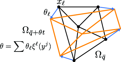
Figure 3. Domain perturbation $\theta$, see Table 3.

6. Example: Poisson equation

To explain the principles of how individual derivatives for forces and target functionals are computed, we use a simple example. For more complex forces in our problem formulation we state the final result in this paper, and we refer to the Appendix for the derivation.

Consider a variable-coefficient Poisson equation $\nabla\cdot(c(x)\nabla u)=f$ and zero Neumann boundary conditions on a domain $\Omega_{\bar{q}}$ that can be changed by the optimization. We take as the optimization objective the squared gradient of the solution on the domain. Then

• the optimization parameters are $q=[{\bar{q}},c]$;

• The PDE in weak form is

  $$\mathcal{H}(u,q,w)=\mathcal{H}(u,{\bar{q}},c,w)=\int_{\Omega_{\bar{q}}}c\nabla u\nabla w-fw\,dx.$$

• The objective is

  $$J(u,{\bar{q}})=\int_{\Omega_{\bar{q}}}\|\nabla u\|^{2}dx.$$

Discretizing in FE basis, with basis functions $\hat{\phi}^{\ell}$ (e.g., quadratic) used for $u=\sum_{\ell}u_{\ell}\hat{\phi}^{\ell}$ and $c=\sum_{\ell}c_{\ell}\hat{\phi}^{\ell}$, and basis $\hat{\xi}^{\ell}$ used for the geometric map ${\mathbf{{\bar{q}}}}=\sum_{\ell}x_{\ell}\hat{\xi}^{\ell}$, we obtain the following. (Note that both our basis $\hat{\xi}$ and $\hat{\phi}$ are defined on the fixed triangulated domain $\Omega_{\mathrm{ref}}$.)

• $\mathbf{q}=[{\mathbf{{\bar{q}}}},\mathbf{c}]=[x_{1}\ldots x_{n_{N}},c_{1}\ldots c_{n_{N}}]$, where $x_{\ell}\in\mathbb{R}^{2}$ are vertices of the physical domain $\Omega_{{\mathbf{{\bar{q}}}}}$, which we optimize, and $c_{\ell}$ are the coefficients of $c$ in FE basis.

• The PDE discretization is performed on the physical domain $\Omega_{\mathbf{{\bar{q}}}}$, and has the form $\mathbf{h}(\mathbf{u},\mathbf{q})=S(\mathbf{q})\mathbf{u}-M(\mathbf{q}){\textbf{f}}$. The entry $(m,\ell)$ of the matrix $S(\mathbf{q})$ are obtained by substituting ${\textbf{u}}=\phi^{m}\circ g^{-1}$ and $w=\phi^{\ell}\circ g^{-1}$, and the discrete expression for $c$ into the expression below; entries of $M(\mathbf{q})$ are obtained in a similar way

  (16) $$S(u,w)=\int_{\Omega_{\mathbf{{\bar{q}}}}}c({\mathbf{{\bar{q}}}}^{-1}(x))\nabla u\cdot\nabla w\,dx;\quad M(v,w)=\int_{\Omega_{\mathbf{{\bar{q}}}}}vw\,dx.$$

• The discrete objective is $J(\mathbf{u},\mathbf{q})=\mathbf{u}^{T}T(\mathbf{q})\mathbf{u}$, with entries of $T(\mathbf{q})$ also obtained by substituting pairs of basis functions into the bilinar form

  (17) $$T(u,w)=\int_{\Omega_{\mathbf{{\bar{q}}}}}\nabla u\cdot\nabla w\,dx.$$

Computing derivatives of $S$, $\partial_{c_{k}}S(u,w)$, with respect to $c$ is straightforward, as the dependence on the coefficients of $c$ is linear. Computation of shape derivatives is more complex, as the integration domain and the gradient operator $\nabla$ with respect to physical domain variables are affected by the change of shape parameters.

Direct approach

The direct approach is to perform a change of variables in (16) and (17) and to the domain $\Omega_{\mathrm{ref}}$, and differentiate with respect to $x_{\ell}$; e.g.,(16) becomes

$$S(u,w)=\int_{\Omega_{\mathrm{ref}}}c(y)\,\nabla_{y}\hat{u}^{T}(\nabla_{y}{\bar{q}})^{-1}(\nabla_{y}{\bar{q}})^{-T}\nabla_{y}\hat{w}\,\,\det\nabla{\bar{q}}\,\,dy,$$

where $\hat{u}$ and $\hat{w}$ denote compositions $u\circ{\bar{q}}^{-1}$. These expressions are highly nonlinear in $x_{\ell}$ and the final expressions for $\partial_{x_{\ell}}S(u,w)$ needed for $\partial_{{\mathbf{{\bar{q}}}}}\mathbf{h}$ are unwieldy, especially for more complex forces like nonlinear elasticity and friction.

Shape derivative approach

Instead, we use shape derivative calculus commonly used in shape optimization to obtain the derivatives with respect to the shape parameters directly on the physical domain $\Omega_{\mathbf{{\bar{q}}}}$ (for the parameters not affecting domain shape the approaches using $\Omega_{\mathrm{ref}}$ and $\Omega_{\mathbf{{\bar{q}}}}$ are identical).

To compute $\partial_{\mathbf{q}}h$, or $\partial_{\mathbf{q}}J$, we consider the perturbed domain $\Omega_{{\mathbf{{\bar{q}}}}+\bm{\theta}\epsilon}$, where $\bm{\theta}$ is a vector field, and compute the full derivative as limit of

$$\frac{1}{\epsilon}\mathopen{}\mathclose{{}\left(h(u_{{\mathbf{{\bar{q}}}}+\bm{\theta}\epsilon},{\mathbf{{\bar{q}}}}+\bm{\theta}\epsilon)-h(u_{{\mathbf{{\bar{q}}}}},{\mathbf{{\bar{q}}}})}\right),$$

as $\epsilon\rightarrow 0$. In the resulting expression, the terms not containing the change $\delta u(x)$ correspond to $\partial_{\mathbf{q}}J\bm{\theta}$, and the terms containing derivatives of $u(x)$ are transformed to $\partial_{\mathbf{u}}J\bm{\psi}$ by substituting $\psi$ instead of $\delta u(x)$.

7. Parametric derivatives of forces

In this section, we derive expressions for $\partial_{\mathbf{u}}\mathbf{h}$ and $\partial_{\mathbf{q}}\mathbf{h}$ for specific forces needed for the adjoint equations and the final derivative formula respectively.

For each force, we obtain expressions of the forms $B$ and $A$ below, from which the matrices for corresponding derivatives can be obtained using:

(18) $$B^{k}(p,\theta)=\mathbf{p}^{T}\partial_{\mathbf{q}}\mathbf{h}^{k}\,\bm{\theta},\;A^{k}(p,\psi)=\mathbf{p}^{T}\partial_{\mathbf{u}}\mathbf{h}^{k}\bm{\psi},$$

with $\theta$ going over basis vectors for this parameter type, $p$ going over adjoint variable components, and $\psi$ over the test function basis vectors for the adjoint; i.e., two matrices of size $D_{s}n_{N}^{z}\times D_{s}n_{N}^{z}$.

While nonlinear elasticity derivatives with respect to material parameters and initial conditions were used in (Geilinger et al., 2020) and (Hahn et al., 2019), and static-problem shape derivatives for a different (static, allowing interpenetration) contact and friction model were obtained in (Tozoni et al., 2021), we present expressions for all force-related derivatives with respect to all parameters (material, shape, initial conditions) in a unified way, simplifying adding additional forces, building whenever possible on a general form described in Section 7.1.

7.1. Volume forces

Many forces in continuum mechanics have the general weak form

(19) $$\mathcal{H}^{v}(u,w,q)=\int_{\Omega_{\mathbf{{\bar{q}}}}}f^{v}(\nabla u,q):\nabla w\,dx,$$

where $u$ is the displacement vector, with the components of the vector $\mathbf{h}^{v}(\mathbf{u})$ obtained as $\mathcal{H}^{v}(u,\phi^{\ell},q)$, for all basis functions $\phi^{\ell}$, and the column denotes tensor contraction. In our case, elastic forces, irrespective of the constitutive law used, belongs to this category.

In these expressions $f^{v}(\nabla u,q)$ is a tensor of dimension $D_{d}\times D_{s}$; e.g., for elasticity, $D_{d}=D_{s}$, and this expression is the stress tensor, as a function of $\nabla u$.

If the force is associated with a volume energy density $W^{v}(\nabla u,q)$, associated forces have the form above, specifically, $f^{v}(\nabla u,q)=\nabla_{1}W^{v}$. (Here, $\nabla_{1}$ means the gradient with respect to the first parameter, which in this case is $\nabla u$). For a surface energy density $W^{s}(u,q)$, the formulas are similar, but the integrals are over the surface.

We also formulate damping forces in a similar way, as explained in more detail below, except at each timestep $W^{v}$ depends on displacements $u^{i}$ and $u^{i-j}$, $j=1\ldots m$ at the current and $m$ previous steps, where $m$ is the order of approximation of velocity used in damping (we use $m=1$). The formulas for $A^{v}$ and $B^{v}$ in this case are obtained in exactly the same way as for the dependence on $u^{i}$ only, separately for $u^{i}$ and $u^{i-1}$, corresponding to $\partial_{\mathbf{u}_{i}}\mathbf{h}^{i}$ and $\partial_{\mathbf{u}_{i-1}}\mathbf{h}^{i}$ respectively.

To obtain matrices $A^{v}$ and $B^{v}$ corresponding to $\partial_{\mathbf{u}}\mathbf{h}^{v}$ and $\partial_{\mathbf{q}}\mathbf{h}^{v}$ (18), we split $\partial_{\mathbf{q}}\mathbf{h}^{f}$ into $\partial_{{\mathbf{{\bar{q}}}}}\mathbf{h}^{f}$ and $\partial_{\mathbf{q}^{1}}\mathbf{h}^{f}$, the shape and non-shape parameter derivatives, assuming $f$ depends on a single volume vector of parameters $q=\mathbf{q}^{1}$ (e.g., Lame constants). We treat these two types of parameters separately, as ${\mathbf{{\bar{q}}}}$ affects the domain of integration but not the integrand, and conversely, $q$ affects the integrand but not the domain.

Shape derivatives

For the shape derivative contribution, we obtain the following forms (the derivation and explicit form of matrix entries can be found in supplementary material).

(20) $$\begin{split}B^{v}(\theta,p)=&\int_{\Omega_{\mathbf{{\bar{q}}}}}-f(\nabla u)\nabla\theta^{T}:\nabla p\\ &-(\nabla_{1}f(\nabla u):(\nabla u\nabla\theta)):\nabla p+\mathopen{}\mathclose{{}\left(f(\nabla u):\nabla p\,}\right)\nabla\cdot\theta\,\,dx,\end{split}$$

$B^{v}(\theta,p)$ is linear in $\theta$ and $p$, and we convert it to a matrix form by substituting basis functions for $\theta$ and $p$.

The contribution to the left-hand side of the adjoint equation is

(21) $$A^{v}(\psi,p)=\int_{\Omega_{\mathbf{{\bar{q}}}}}(\nabla_{1}f(\nabla u):\nabla\psi):\nabla p\,dx.$$

Observe that the matrix is identical to the matrix used in the forward solve.

Non-shape volumetric parameter derivatives

We assume that the force depends on $q=q(x)$, a function of the point in $\Omega_{\mathbf{{\bar{q}}}}$, defined by its values $\mathbf{q}$ at the same nodes as the solution, and interpolated using the same basis $\phi$.

In this case, the form $B$ is:

$$B^{v}(\theta,p)=\int_{\Omega}(\partial_{q}f\cdot\theta):\nabla p\,\,dx.$$

The contribution to the left-hand side of the adjoint equation is identical to the shape derivative case.

In our implementation we consider two versions of elastic forces, both defined by Lame parameters specified as functions on $\Omega_{\mathrm{ref}}$: $q(x)=[\lambda(x),\mu(x)]$. The only quantities we need are derivatives of $f(\nabla u)$ with respect to $\nabla u$, and material parameters.

Linear elasticity

For linear elasticity, we replace $f^{v}$ with

$$f^{e}(\nabla u,\mathbf{q})=\sigma(\nabla u,\mathbf{q})=C(\mathbf{q}):\varepsilon(\nabla u)=\frac{1}{2}\,C(\mathbf{q}):(\nabla u^{T}+\nabla u),$$

with $C_{ijkl}(\lambda,\mu)=\lambda\delta_{ij}\delta_{kl}+\mu(\delta_{ik}\delta_{jl}+\delta_{il}\delta_{jk})$.

For computing $A^{e}$ and $B^{e}$ we use partial derivatives of $f^{e}$ with respect to material parameters:

$$\nabla_{1}f^{e}(\nabla u,\bm{\lambda},\bm{\mu}) =C,$$

$$\partial_{\lambda}f^{e}(\nabla u,\bm{\lambda},\bm{\mu})_{ij} =\delta_{ij}\delta_{kl}\varepsilon_{kl},$$

$$\partial_{\mu}f^{e}(\nabla u,\bm{\lambda},\bm{\mu})_{ij} =(\delta_{ik}\delta_{jl}+\delta_{il}\delta_{jk})\varepsilon_{kl}.$$

Neo-Hookean elasticity

For Neo-Hookean elasticity, the following formula is used for computing stress from the deformation gradient:

$$f^{e}(\nabla u,\mathbf{q})=\mu(F(\nabla u)-Q(\nabla u))+\lambda\log(\det(F(\nabla u)))\,Q(\nabla u),$$

where $F(\nabla u)=\nabla u+I$ and $Q(\nabla u)=F(\nabla u)^{-T}$.

We can then compute derivatives of $f(\nabla u)$:

$$\nabla_{1}f^{e}(\nabla u,\mathbf{q})_{ijkl} =\mu(\delta_{ik}\delta_{jl}+Q_{il}Q_{kj})$$

$$\quad+\lambda(Q_{ij}Q_{kl}-\log(\det(F))\,Q_{il}Q_{kj}),$$

$$\partial_{\lambda}f^{e}(\nabla u,\mathbf{q}) =F(\nabla u)-Q(\nabla u),$$

$$\partial_{\mu}f^{e}(\nabla u,\mathbf{q}) =\log(\det(F(\nabla u)))\,Q(\nabla u).$$

Damping

For damping, we have material parameters controlling shear and bulk damping $\alpha,\beta$. We use the strain-rate proportional damping described in  (Brown et al., 2018). Given deformation gradient $F=\nabla u+I$, the Green strain tensor $E=\frac{1}{2}(F^{T}F-I)$ is rotation-invariant. The viscous Piola-Kirchhoff stress is of the form

$$P(\nabla u,\nabla\dot{u})=F(2\alpha\dot{E}+\beta\operatorname{Tr}\small(\dot{E}\small)I),$$

where $\dot{E}$ denotes the time derivative, and the weak form of the corresponding force

$$\mathcal{H}^{d}(u,\dot{u},w)=\int_{\Omega_{\mathbf{{\bar{q}}}}}P(\nabla u,\nabla\dot{u})\nabla wdx.$$

In our case, to fit this force into our differentiable formulation, we discretize $\dot{F}$ using as $\dot{F}^{i}=\frac{1}{\Delta t\,}(F^{i}-F^{i-1})$; this yields a force expression of the form

$$\mathcal{H}^{d}(u^{i},u^{i-1},w)=\int_{\Omega_{\mathbf{{\bar{q}}}}}P(\nabla u^{i},\nabla u^{i-1})\nabla wdx,$$

which is identical to (19), except it depends on both $\nabla u^{i}$ and $\nabla u^{i-1}$. As a consequence, expressions for $A^{d}(\psi,p)$ and $B^{d}(\theta,p)$ are obtained in the same way as in (21) and (20), except two pairs of matrices are obtained, one for $\nabla u^{i}$ the other for $\nabla u^{i-1}$, using $\nabla_{1}P$ and $\nabla_{2}P$ as $\nabla_{1}f$ respectively.

7.2. Contact and Friction

For the contact forces, we use a slightly modified version of the formulation of (Li et al., 2020). While the original formulation is introduced in a discrete form, it can be derived with minimal changes as a linear finite-element discretization of a continuum formulation (Li et al., 2023). The contact incremental potential uses log barrier function $b(y)$, where $b$ is a truncated log barrier function, approaching infinity, if $y\rightarrow 0$, and vanishing for $y\geqslant\hat{d}$ for some small distance $\hat{d}$.

For any pair $k$ of primitives (vertices, edges, and faces) of the surface mesh $\partial\Omega_{\mathbf{x}^{d}}$, defined by the vertex positions $\mathbf{x}^{d}=M^{*}{\mathbf{{\bar{q}}}}+\mathbf{u}$, $d_{k}(\mathbf{x^{d}})$ denotes the distance between them; $C$ is the set of primitive pairs in contact, i.e., pairs of primitives with $d_{k}<\hat{d}$.

Recall that the geometric map ${\bar{q}}$ always uses piecewise-linear elements $\xi_{\ell}$, while the basis for the deformations $u$ can be of any order. The matrix $M^{*}$ is an upsampling matrix to bring dimension of ${\mathbf{{\bar{q}}}}$ to the same as discrete solution $\mathbf{u}$. The upsampling is performed by linear interpolation from $\hat{x}_{\ell}$ to nodes $\hat{z}_{\ell}$.

The contact forces are derived from the following potential:

$$E(\mathbf{u},{\mathbf{{\bar{q}}}})=\kappa\sum_{k\in C}b(d_{k}(\mathbf{x}^{d}))A_{k}=\sum_{k\in C}W_{k}(\mathbf{u},{\mathbf{{\bar{q}}}})A_{k},$$

where $\kappa>0$ is a parameter controlling the barrier stiffness and $A_{k}$ corresponds to the sum of surface areas associated with each primitive in $k$ (i.e., $\tfrac{1}{3}$ of the sum of areas of incident triangles for vertices and edges, and the area for triangles). See Section D in the Appendix.

We define $F^{c}_{k}(\mathbf{u},{\mathbf{{\bar{q}}}})=\partial_{\mathbf{u}}W_{k}(\mathbf{u},{\mathbf{{\bar{q}}}})=\kappa b^{\prime}(d_{k}(\mathbf{x}^{d}))\partial_{\mathbf{x^{d}}}d_{k}$.

The contact force is given by

$$\mathbf{h}^{c}=\sum_{k\in C}F^{c}_{k}(\mathbf{u},{\mathbf{{\bar{q}}}})A_{k}.$$

The terms $B^{c}$ and $A^{c}$ have the form

$$B^{c}(p,\theta) =\sum_{k}\mathopen{}\mathclose{{}\left(\partial_{\mathbf{{\bar{q}}}}F^{c}_{k}\theta\cdot p+F^{c}_{k}\cdot p\,\,\partial_{\mathbf{{\bar{q}}}}A_{k}}\right)A_{k},$$

$$A^{c}(p,\psi) =\sum_{k}\partial_{\mathbf{u}}F^{c}_{k}\psi\cdot p\,\,A_{k},$$

where

$$\partial_{\mathbf{u}}F^{c}_{k} =\kappa\large(b^{\prime\prime}(\partial_{\mathbf{x^{d}}}d_{k})(\partial_{\mathbf{x^{d}}}d_{k})^{T}+b^{\prime}\partial_{\mathbf{x^{d}}}(\partial_{\mathbf{x^{d}}}d_{k})\large),$$

$$\partial_{\mathbf{{\bar{q}}}}F^{c}_{k} =\partial_{\mathbf{u}}F^{c}_{k}M^{*}$$

and $\partial_{\mathbf{{\bar{q}}}}A_{k}$ corresponds to the gradient of the area term, which varies depending on the type of primitive pairs corresponding to $k$. See Section D in the Appendix.

Friction

In general, the friction coefficient $\gamma(x_{1},x_{2})$ is a function of pairs of surface material points in $\partial\Omega_{\mathbf{{\bar{q}}}}$. As a simplification, in our implementation, we assume that each pair of objects $(m,n)$, in the simulation has a single coefficient $\gamma_{m,n}$, which can vary through the optimization. To simplify notation, we use $\gamma_{k_{1},k_{2}}$ for a pair of primitives $k_{1}$ and $k_{2}$ to indicate the friction coefficient between objects these primitives belong to.

We follow the IPC definition of friction (Li et al., 2020). Its key feature is that it is a differentiable function of displacements, which determine the contact forces, and relative velocities, which, for dynamic problems, we discretize using first-order approximation $u^{i}-u^{i-1}$, where $i$ is the time step.

The friction force for each active pair of primitives $k$ is

(22) $$F^{f}_{k}(\mathbf{u}^{i-1},\mathbf{u}^{i})=-\gamma_{k_{1},k_{2}}N_{k}T_{k}f_{\eta}(\lVert\tau_{k}\rVert)\frac{\tau_{k}}{\lVert\tau_{k}\rVert},$$

where $N_{k}$ is the contact force magnitude, $T_{k}$ is a tangential frame matrix, constructed as described in (Li et al., 2020), and $\tau_{k}$ and $f_{\eta}$ are defined as

$$\tau_{k} =T_{k}(\mathbf{x}^{d,i-1})^{T}(\mathbf{u}^{i}-\mathbf{u}^{i-1}),$$

$$f_{\eta}(y) =\begin{cases}-\frac{y^{2}}{\eta^{2}}+\frac{2y}{\eta}&y\in[0,\eta)\\ 1&y\geqslant\eta\end{cases}.$$

The total friction force has the form

$$\mathbf{h}^{f}=\sum_{k\in C}F^{f}_{k}(\mathbf{u}^{i},\mathbf{u}^{i-1},{\mathbf{{\bar{q}}}})\,A_{k},$$

with the form $B$ for shape derivatives given by

$$B^{f}(p,\theta)=\sum_{k}\partial_{\mathbf{{\bar{q}}}}F^{f}_{k}\theta\cdot p\,A_{k}+F^{f}_{k}\cdot p\,\,\partial_{\mathbf{{\bar{q}}}}A_{k}\,\,A_{k}.$$

Additional details on the computation of $\partial_{\mathbf{{\bar{q}}}}F^{f}_{k}$ are in the Appendix (Section E). The derivative with respect to friction coefficient values is easily obtained as the force is linear in friction coefficients. If $\mathbf{q}$ is a vector of friction coefficients,

$$\partial_{q_{\ell}}F^{f}_{k}=\begin{cases}-N_{k}T_{k}f_{\eta}(\lVert\tau_{k}\rVert)\frac{\tau_{k}}{\lVert\tau_{k}\rVert}&\text{if $q_{\ell}$ corresponds to $\gamma_{k_{1},k_{2}}$}\\ 0&\text{otherwise}.\\ \end{cases}$$

Two forms $A^{f}$, for $\partial_{\mathbf{u}_{i}}$ and $\partial_{\mathbf{u}_{i-1}}$ are needed for the adjoint equation. Both have the general form

$$A^{f}(\psi,p)=\sum_{k}\partial_{\mathbf{u}}F_{k}\psi\cdot p\,\,A_{k},$$

which reduces to computing the derivative of each $F_{k}$ term with respect to $u^{i}$ and $u^{i-1}$, which can be be found in Appendix E.

8. Objective derivatives

In this section, we define the $\partial_{\mathbf{q}}J$ and $\partial_{\mathbf{u}}J$ terms needed for the gradient computation (10): For each objective-optimization parameter pair, $\partial_{\mathbf{q}}J^{\ell}\,\bm{\theta}$ and $\partial_{\mathbf{u}}J^{\ell}\bm{\psi}$, i.e., two vectors of size $D_{s}n_{N}^{z}$.

Similar to Section 7, we present all objective derivatives with respect to all types of optimization parameters, including shape in a unified way. We consider a comprehensive set of objectives used in many previous works, that can be easily extended with additional ones. In Section 8.1 we present general forms that all objectives can be reduced to.

8.1. General forms of objectives

Typically, objectives do not depend directly on the optimization parameters other than shape, so we focus primarily on derivatives of objectives with respect to shape parameters ${\mathbf{{\bar{q}}}}$ and solution $\mathbf{u}$.

We consider objectives of the form

(23) $$J(\mathbf{u},{\mathbf{{\bar{q}}}})=J(J_{1}(\mathbf{u},{\mathbf{{\bar{q}}}}),\ldots J_{n_{J}}(\mathbf{u},{\mathbf{{\bar{q}}}})),$$

where $J$ is a differentiable function, and $J_{i}$, $i=1\ldots n_{J}$ are objective terms each of which typically has one of the integral forms described below. $J$ can be as simple $J(J_{1})=J_{1}$, or can depend on several terms, as e.g., the center of mass optimization. The derivatives of objective are reduced to the the derivatives of the objective terms by a direct application of a chain rule, so we focus on these.

We first consider two general forms of objective terms which will be used for a number of specific objectives in Section 8.2. This includes inequality constraints in penalty form.

For each objective term $J^{o}$, we obtain vectors $R^{o}(\psi)$ and $S^{o}(\theta)$ corresponding to the partial derivatives $\partial_{\mathbf{u}}J^{o}$ and $\partial_{\mathbf{q}}J^{o}$, which are necessary to compute the adjoint solution and the full shape derivative. As for the derivatives of the objective vectors $\partial_{\mathbf{u}}J^{o}$ and $\partial_{\mathbf{q}}J^{o}$ are obtained by plugging in the basis functions $\phi_{\ell}$ int $R^{o}$ and $S^{o}$.

Objectives depending on gradient of solution and shape

Consider an objective term that depends on both the solution of the PDE and the domain:

(24) $$J^{o}(\nabla u,{\bar{q}})=\int_{\Omega_{\mathbf{{\bar{q}}}}}j(\nabla u,x)dx.$$

In this case, as derived in the supplementary document,

(25) $$S^{o}(\theta)=\int_{\Omega_{\mathbf{{\bar{q}}}}}-\nabla_{1}j:\nabla u\,\nabla\theta+\nabla_{2}j\cdot\theta+j\nabla\cdot\theta\,\,dx$$

and

(26) $$R^{o}(\psi)=\int_{\Omega_{\mathbf{{\bar{q}}}}}\nabla_{1}j:\nabla\psi\,\,dx.$$

Objective terms depending on solution and shape

We also use objective terms depending on both the solution of the PDE and the domain:

(27) $$J^{o}(u,{\bar{q}})=\int_{\Omega_{\mathbf{{\bar{q}}}}}j(u,x)dx.$$

In this case,

(28) $$S^{o}(\theta)=\int_{\Omega_{\mathbf{{\bar{q}}}}}\nabla_{2}j\cdot\theta+j\nabla\cdot\theta\,\,dx$$

and

(29) $$R^{o}(\psi)=\int_{\Omega_{\mathbf{{\bar{q}}}}}\nabla_{1}j\cdot\psi\,\,dx.$$

8.2. Specific objectives

$L_{p}$ norm of stress

For $p=2$ this objective measures the overall average stress, and for high $p$, $L_{p}$-norm of stress approximates maximal stress:

(30) $$J^{\sigma}=\mathopen{}\mathclose{{}\left(\int_{\Omega_{\mathbf{{\bar{q}}}}}\|\sigma(\nabla u)\|_{F}^{p}dx}\right)^{1/p},$$

where $\sigma(\nabla u)=f(\nabla u)$ represents stress, which depends on $\nabla u$. Following the chain rule, this objective is a function of a single objective term $J^{\sigma}=(J_{1}^{\sigma})^{p}$ which is of the form (24). with $j=\|\sigma(\nabla u)\|_{F}^{p}$ for which $\nabla_{2}j=0$, and

$$\nabla_{1}j =p\,\|\sigma\|^{p-2}\,\,\sigma\,:\,\nabla f(\nabla u).$$

Weighted difference from target deformations

(31) $$J^{trj}(x,u)=\int_{\Omega_{\mathbf{{\bar{q}}}}}w({\bar{q}}^{-1}(x))\,\,\|x^{d}-x^{trg}({\bar{q}}^{-1}(x))\|^{2}\,\,dx$$

where $x^{d}=x+u$, the deformed state of the object, weight $w$ determines relative importance of points, and $x^{trg}$ is the target configuration, defined as function on $\Omega_{\mathrm{ref}}$.

The formulas for the general objective (27), apply, with

$$\nabla_{1}j=\nabla_{2}j=2w({\bar{q}}^{-1}(x))(x^{d}-x^{trg}({\bar{q}}^{-1}(x)).$$

If we define only the shape on the boundary as the target, then we have:

$$J^{btrj}=\int_{\partial\Omega_{\mathbf{{\bar{q}}}}}w({\bar{q}}^{-1}(x))\,\,\|x^{d}-x^{trg}({\bar{q}}^{-1}(x))\|^{2}\,\,dx$$

. Formulas for the derivatives are similar:

$$S^{btrj}=\int_{\partial\Omega_{\mathbf{{\bar{q}}}}}\nabla_{2}j\cdot\theta+j(u,x)\,\nabla_{s}\cdot\theta\,\,dx,$$

$$R^{btrj}=\int_{\partial\Omega_{\mathbf{{\bar{q}}}}}\nabla_{1}j\cdot\psi\,\,dx,$$

where $\nabla_{s}$ denotes the surface derivative.

Target center of mass trajectory

A related objective is the deviation of the center of mass of the object from a target trajectory.

(32) $$J^{ctr}(J^{P},J^{D}) =\bigg{\lVert}\frac{J^{P}}{J^{D}}-x^{ctr}\bigg{\rVert}^{2}=\bigg{\lVert}\frac{\int_{\Omega_{\mathbf{{\bar{q}}}}}\rho(x)\,x^{d}\,dx}{\int_{\Omega_{\mathbf{{\bar{q}}}}}\rho(x)\,\,dx}-x^{ctr}\bigg{\rVert}^{2}$$

$$=\sum_{i}^{D_{d}}\mathopen{}\mathclose{{}\left(\frac{J^{P}_{i}}{J^{D}}-x^{ctr}_{i}}\right)^{2}.$$

Using the chain rule, we can reach a formulation where $S^{ctr}$ and $R^{ctr}$ depend on respective derivatives from each $J^{P}_{i}$ and $J^{D}$:

$$S^{ctr}=\sum_{i}(\partial_{1}J^{ctr})_{i}S^{P}_{i}+\partial_{2}J^{ctr}S^{D},$$

$$R^{ctr}=\sum_{i}(\partial_{1}J^{ctr})_{i}R^{P}_{i}+\partial_{2}J^{ctr}R^{D}.$$

We then need to compute shape derivative and adjoint terms for both of our scalar integrals $J^{P}_{i}$ and $J^{D}$, following general formulas for 27. For each $J^{P}_{i}$, we have:

$$\nabla_{1}j=\nabla_{2}j=\rho(x)e_{i},$$

where $e_{i}\in\,\mathbb{R}^{D_{d}}$ is a vector with $0$s everywhere except at index $i$, where the value is $1$.

Finally, assuming that densities are constant per point, for $J_{D}$,

$$\nabla_{1}j=\nabla_{2}j=0.$$

Height

This functional aims to maximize the height of the center of mass:

(33) $$J^{z_{\text{max}}}=-\frac{\int_{\Omega_{\mathbf{{\bar{q}}}}}\rho(x)x^{d}_{z}dx}{\int_{\Omega_{\mathbf{{\bar{q}}}}}\rho(x)dx},$$

where $u_{z}$ is the z (vertical) component of the solution (displacement) $u$, $x_{z}$ is the z component of the original position x. We can rewrite this formula using $J^{P}_{z}$ and $J^{D}$ from previous subsection:

(34) $$J^{z_{\text{max}}}(J^{P}_{z},J^{D})=-\frac{J^{P}_{z}}{J^{D}}.$$

This way, similar to $J^{ctr}$, we have:

$$S^{z_{\text{max}}}=\partial_{1}J^{z_{\text{max}}}S^{P}_{z}+\partial_{2}J^{z_{\text{max}}}S^{D},$$

$$R^{z_{\text{max}}}=\partial_{1}J^{z_{\text{max}}}R^{P}_{z}+\partial_{2}J^{z_{\text{max}}}R^{D}.$$

Then, as for previous case, we can compute $S^{P}_{z}$, $R^{P}_{z}$, $S^{D}$ and $R^{D}$ through general formula 27, using $\nabla_{1}j=\nabla_{2}j=\rho(x)e_{z}$ for $J^{P}_{z}$ and $\nabla_{1}j=\nabla_{2}j=0$ for $J^{D}$.

Upper bound for volume

A constraint on the volume of the optimized object in penalty form is

(35) $$J^{V} =\varphi(V(\Omega_{\mathbf{{\bar{q}}}})-V_{t}),$$

where $V$ corresponds to ($\int_{\Omega_{\mathbf{{\bar{q}}}}}\,dx$), the volume of shape $\Omega_{\mathbf{{\bar{q}}}}$, $V_{t}$ to the target volume, and $\varphi(z)$ is a quadratic penalty function equal to $z^{2}$ for positive $z$ and zero for negative $z$. This functional reduces to the general objective (27), with $\nabla_{1}j=\nabla_{2}j=0$, since $j(u,x)=1$.

Upper bound for stress

Similarly, we can impose an approximate upper bound on stress via a penalty:

(36) $$J^{\sigma_{t}} =\int_{\Omega_{\mathbf{{\bar{q}}}}}\varphi(\|\sigma\|-s_{t})dx,$$

where $s_{t}$ is the stress magnitude target. As for $L_{p}$ stress energy, our integrand $\varphi(\|\sigma\|-s_{t})$ depends only on $\nabla u$ and (24) applies with

$$\nabla_{1}j =\varphi^{\prime}\,\frac{f(\nabla u)}{\|\sigma\|}\,:\,\nabla f(\nabla u),$$

$$\nabla_{2}j =0.$$

8.3. Regularization terms

In addition to the physical objectives described in the previous sections, we use two discrete regularization terms essential for numerical stability for a number of problems.

Scale-invariant smoothing

(37) $$J^{\text{smooth}}=\sum_{i\in B}\|s_{i}\|^{p},\qquad s_{i}=\frac{\sum_{j\in N(i)\cap B}(v_{i}-v_{j})}{\sum_{j\in N(i)\cap B}\|v_{i}-v_{j}\|},$$

where $B$ contains the indices of all boundary vertices, $N(i)$ contains the indices of all neighbor vertices of vertex $i$, and $v_{i}$ is the position of vertex $i$. The value of $p$ can be adjusted to obtain smoother surfaces at the cost of less optimal shapes, normally we use $p=2$. This term is scale-invariant and pushes the triangles/tetrahedra of the mesh toward equilateral. The derivative of this smoothing term with respect to optimization parameters $v_{i}$ can be seen in the first paragraph of Section F (Appendix).

Material parameter spatial smoothing

(38) $$J^{\lambda,\mu\ \text{smooth}}=\sum_{t\in T}\sum_{t^{\prime}\in Adj(t)}\mathopen{}\mathclose{{}\left(1-\frac{\lambda_{t^{\prime}}}{\lambda_{t}}}\right)^{2}+\mathopen{}\mathclose{{}\left(1-\frac{\mu_{t^{\prime}}}{\mu_{t}}}\right)^{2},$$

where $T$ is the set of all triangles/tetrahedra, $Adj(t)$ is the set of triangles/tetrahedra adjacent to $t$. $\lambda,\mu$ are the material parameters defined per triangle. The derivative of this term can be seen in the last part of Section F (Appendix).

9. Results

We partition our results in three groups depending on the type of the dofs used in the objective function: shape (Section 9.2), initial conditions (Section 9.3), or material (Section 9.4). For each group we provide a set of examples of static and dynamic scenes of increasing complexity. In Section 9.5, we compare our solver, (Du et al., 2021), and (Jatavallabhula et al., 2021) to evaluate the effect of different material and contact models. We also compare against a baseline implementation using finite differences. We run our experiments on a workstation with a Threadripper Pro 3995WX with 64 cores and 512 Gb of memory. For a selection of problems, we validate our results with physical experiments using items fabricated in silicon rubber (we use 1:1 SMOOTH-ON OOMOO 30 poured into a 3D printed PVA mold) or 3D printed PLA plastic.

We additionally provide a video showing the intermediate optimization step for all the results in the paper as part of our additional material.

Statistics

We provide statistics for our experiments in Table 4, including size of the meshes, material model, running time and memory used.

We observe that the time to compute the gradients of the objective function is negligible compared to the forward solve time (usually less than 10%). This implies that as long as a physical system can be simulated in PolyFEM, our approach enables to optimize functionals depending on it with a comparable running time per optimization iteration.

We recall that the gradient computation requires solving one linear system for each time step of the forward simulation. For linear problems, the system to solve has the same stiffness matrix and we can thus reuse the factorization. For non-linear problems requiring Newton iterations, the forward step requires multiple Netwon steps, while the solve for the gradient is always a single linear system solve.

An additional acceleration strategy that we employ is noting that the optimization algorithm needs to solve many, often similar, forward simulations. We thus initialize, for non-linear problems, the forward solver with the solution at the previous step, which is often a good initialization.

Table 4. Columns from left to right are: example names, number of vertices, degree of freedom of the simulation, physical formulation, objective functional of the optimization, total running time (sec), peak memory (Mb), number of iterations of the optimization, average running time of the simulation (sec), average running time of computing gradients (sec), total number of Newton iterations (linear solves) in the simulation, number of Newton solves in the simulation.

Example	Vertices	Dofs	Model	Objective	Total time	Memory	Iter	Solve time	Grad time	Newton Iter.	Newton Solve
Bridge (Figure 5)	4641	9282	Linear	Target	16.1	162.3	55	0.0343	0.0296	0	0
Bridge (Figure 6)	18598	143378	Linear	Stress	1665.8	1690.8	402	1.3859	0.1861	0	0
3D Beam (Figure 7)	9939	209409	NeoHookean	Stress	95738.6	101786.3	171	192.1587	37.2651	1083	361
Interlocking (Figure 8)	1290	9946	IPC	Stress	303.3	188.5	101	0.8394	0.0590	4900	335
2D Hook (Figure 9)	1760	13348	IPC	Stress	220.5	726.5	60	1.7224	0.0802	2548	126
3D Hanger (Figure 10)	4190	80412	IPC	Stress	14129.4	6554.0	29	204.2374	3.2117	4708	64
Bouncing Ball (Figure 11)	73	146	IPC	Target	961.7	29.2	202	1.1061	0.0898	211611	41200
Sliding Ball (Figure 12)	526	6849	IPC	Stress	1610.1	2184.6	29	24.3086	1.2580	0	0
Shock Protection (Figure 13)	53879	107758	IPC	Stress	33301	10100	9	1264.395	129.96	35553	4800
Puzzle Piece (Figure 14)	370	740	IPC	Trajectory	47.4	107.6	19	1.5877	0.2129	2917	630
Throw Bunny (Figure 1)	2174	6522	IPC	Target	602.0	3344.1	9	209.2998	4.3731	15324	1000
Colliding Tentacles (Figure 15)	6896	20688	IPC	Trajectory	13070	8325	5	2043	41.25	14447	720
Sine (Figure 16)	651	1302	Linear	Target	0.3	34.4	12	0.0042	0.0022	0	0
Bridge (Figure 17)	18598	37196	Linear	Target	32.7	655.2	39	0.1416	0.0398	0	0
Cube (Figure 18)	4631	103383	NeoHookean	Target	455.8	6316.6	8	37.9947	2.6101	33	11
Micro-Structure (Figure 19)	3268	9804	IPC	Target	602.3	33502.3	11	42.0954	0.0746	249	14
Kangaroo (Figure 20)	231	462	IPC	Trajectory	21.6	224.6	6	1.6704	0.1624	2987	660
Sliding Bunny (Figure 21)	5682	17046	IPC	Target	11734.0	2304.3	8	547.3644	1.6478	61517	880
Bouncing Ball (Figure 22)	720	1440	IPC	Height	612.3	86.4	79	3.3482	0.2003	33609	5160
Bouncing Ball (Figure 23)	646	1938	NeoHookean	Trajectory	206.3	152.8	24	3.0548	0.7396	3264	1632
Bouncing Ball (Figure 23)	1251	3753	IPC	Trajectory	10546.6	1547.0	49	113.4214	8.8056	105401	20160

Color Legend

We use green arrows to indicate Neumann boundary conditions, and black squares to indicate nodes that have a Dirichlet boundary condition. To reduce clutter, we use a uniform gray to indicate objects with a uniform Dirichlet boundary condition on all nodes.

To avoid singularities in the optimization we add, to the objective function, a boundary smoothing term (37) in all our shape optimization experiments, and a material regularization term (38) to all our material optimization experiments.

9.1. Implementation

FE Solver

We implemented our solver in C++ using the PolyFEM library (Schneider et al., 2019) for the forward solve, the IPC Toolkit (Ferguson et al., 2020) for computing contact and friction potentials, and Pardiso (Alappat et al., 2020; Bollhöfer et al., 2020, 2019) for solving linear systems.

Optimization

Our optimization algorithm (Algorithm 1) uses the L-BFGS implementation in (Wieschollek, 2016), with backtracking line search.

Meshing

Shape optimization might negatively affect the element shape, and for large deformation introduce close to singular elements that force the optimization to take tiny steps. After every optimization iteration, we evaluate the element quality using the scaled Jacobian quality measure (Knupp, 2001), and we optimize the mesh if it is below a threshold experimentally set to $10^{-3}$.

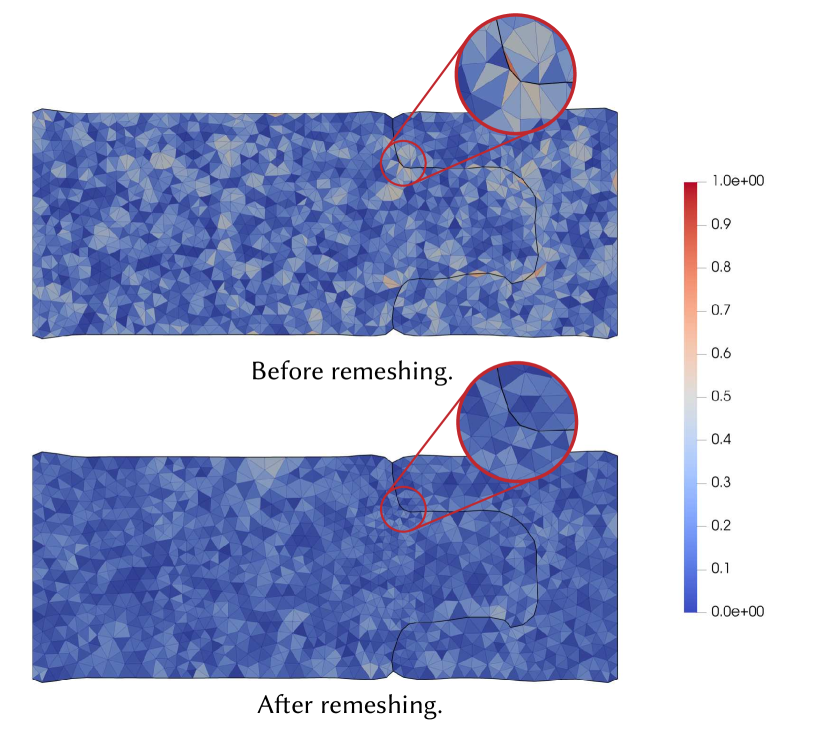
Figure 4. An example of remeshing in the shape optimization. The quality is shown for each triangle. Triangles with bad quality have higher values.

For 2D examples, we keep the mesh boundary fixed and we regenerate the interior using GMSH (Geuzaine and Remacle, 2009) (Figure 4). For 3D examples, we similarly fix the boundary and then use the mesh optimization procedure of fTetWild (Hu et al., 2020) to improve the quality of the interior until its quality is above the threshold.

The reason for fixing the boundary is that our optimization objectives (Section 8.1) often depend on quantities on the boundary: if the boundary is remeshed, we will need a bijective map between the two boundaries. Meshing methods providing this map exist (Jiang et al., 2020), but their integration in our framework, while trivial from a formulation point of view, is an engineering challenge that we leave as future work.

Reproducibility

The reference implementation of our solver and applications will be released as an open-source project.

9.2. Shape Optimization

We start our analysis with shape optimization problems both without and with contact or friction forces.

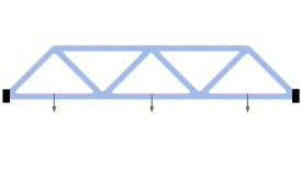
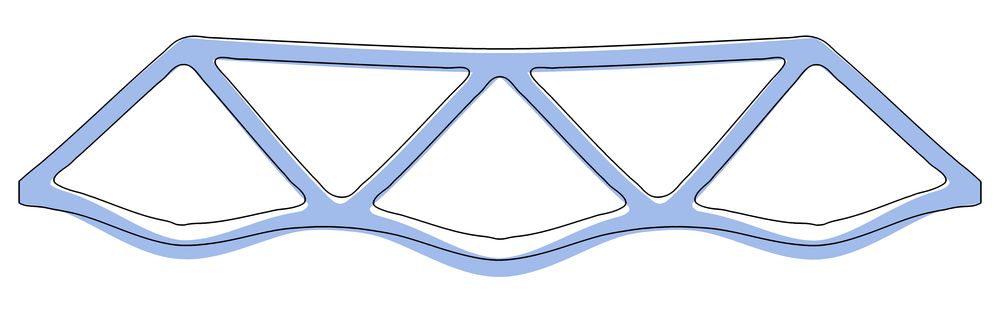
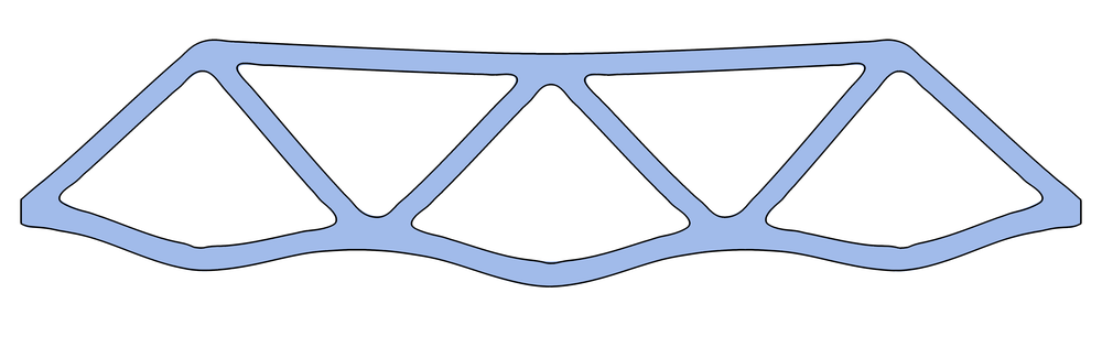
Problem setup.

Initial shape.

Optimized shape.

Figure 5. Static: Bridge With Fabricated Solution. The result of the shape optimization (blue surface) matches the target shape (wire-frame).

Static: Bridge With Fabricated Solution

We fabricate a 2D solution to verify the correctness of our formulation and implementation. Starting from the shape of a bridge (Figure 5) we run a forward linear elasticity simulation with the two sides fixed and gravity forces. We now perturb the geometry of the rest pose and solve a shape optimization problem to recover the original rest pose, i.e. we remove the perturbation we introduced by minimizing the objective in (31).

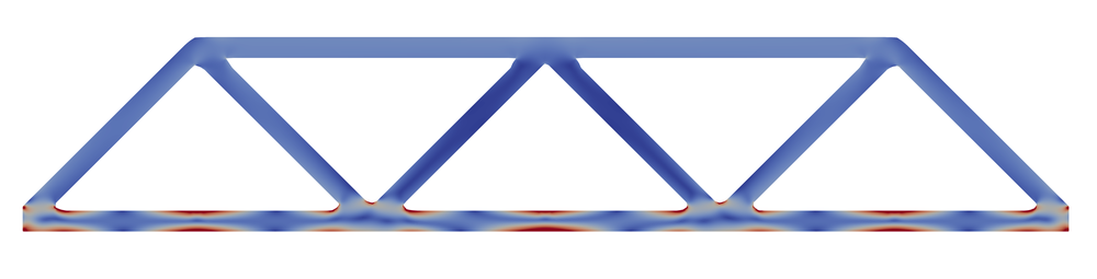
Initial stress distribution.

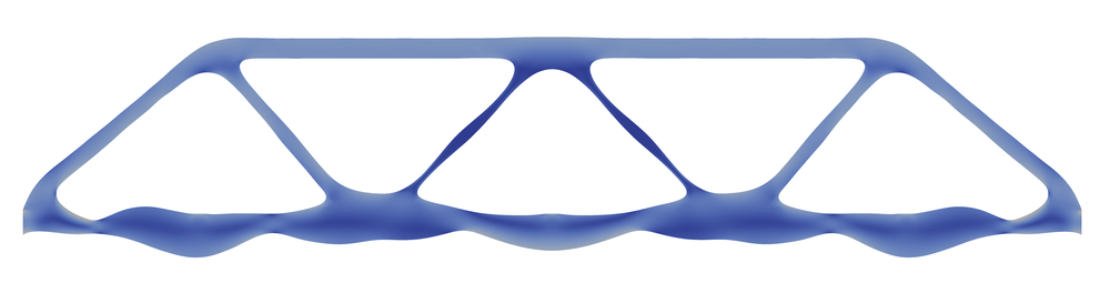
Optimized stress distribution.

Figure 6. Static: Bridge. Result of shape optimization to minimize the average stress.

Static: Bridge

We use the same model for a more challenging problem (Figure 6): we use the same Dirichlet conditions and material model, replace the gravity forces by 3 Neumann conditions on the lower beams, and minimize the $L^{8}$ norm of stress (30). To avoid trivial solutions we add a constant volume constraint (Section 8.2). The maximum stress is reduced from $68.789$ to $22.232$.

Static: 3D Beam

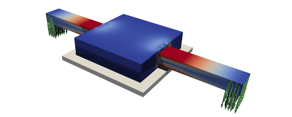
Initial stress distribution.

Optimized stress distribution.

Figure 7. Static: 3D Beam. Result of stress minimization on a beam standing on a platform, with two loads on its sides.

Moving to 3D (Figure 7), we perform static optimization of the $L^{8}$ norm of stress using Neo-Hookean materials on a beam standing on a fixed support at the center (nodes on the bottom surface of the beam have zero Dirichlet boundary conditions), and with two side loads applied as Neumann boundary conditions. We use (35) to bound the volume of the beam during optimization in order to avoid trivial solutions. The maximum stress is reduced from $3,377$ to $920$. Note that this scene is not using contact, the lower region of the central part of the beam is fixed with Dirichlet boundary conditions.

Static: Interlocking

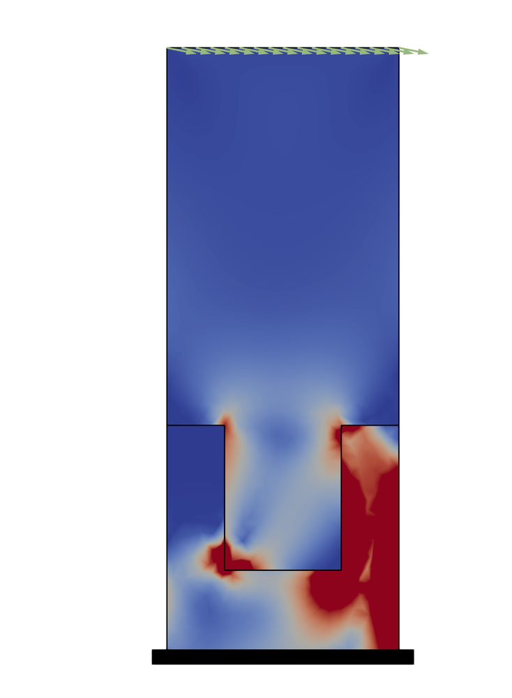
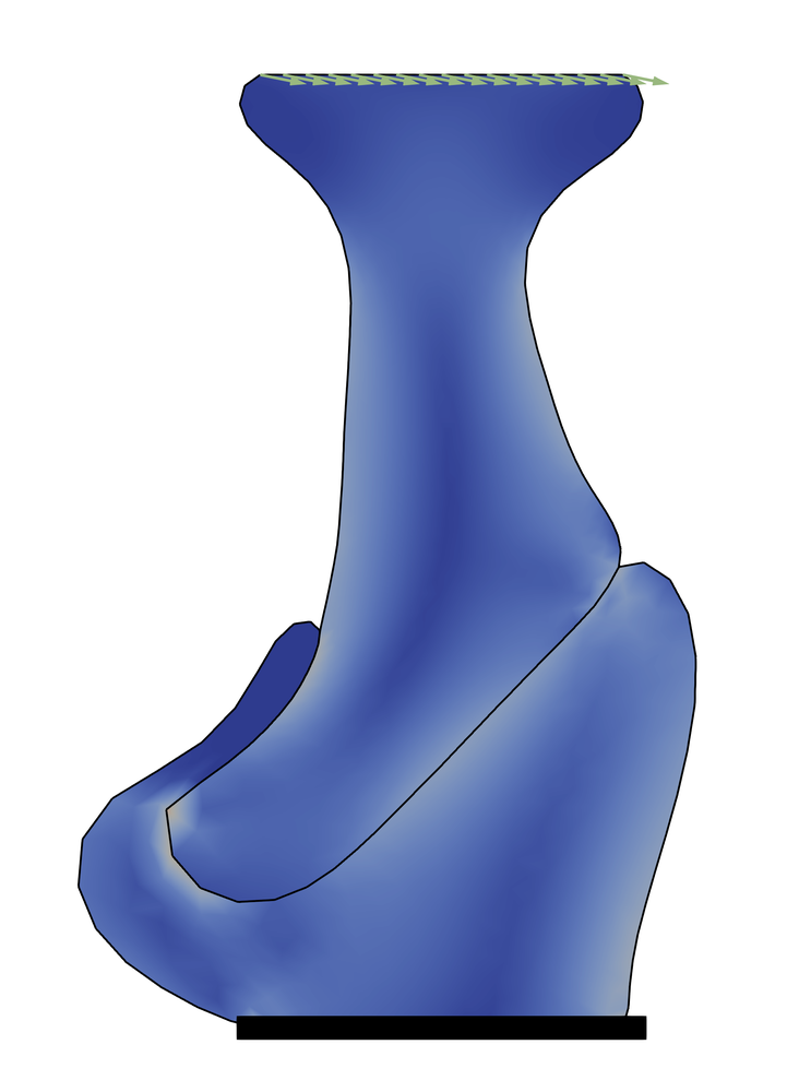
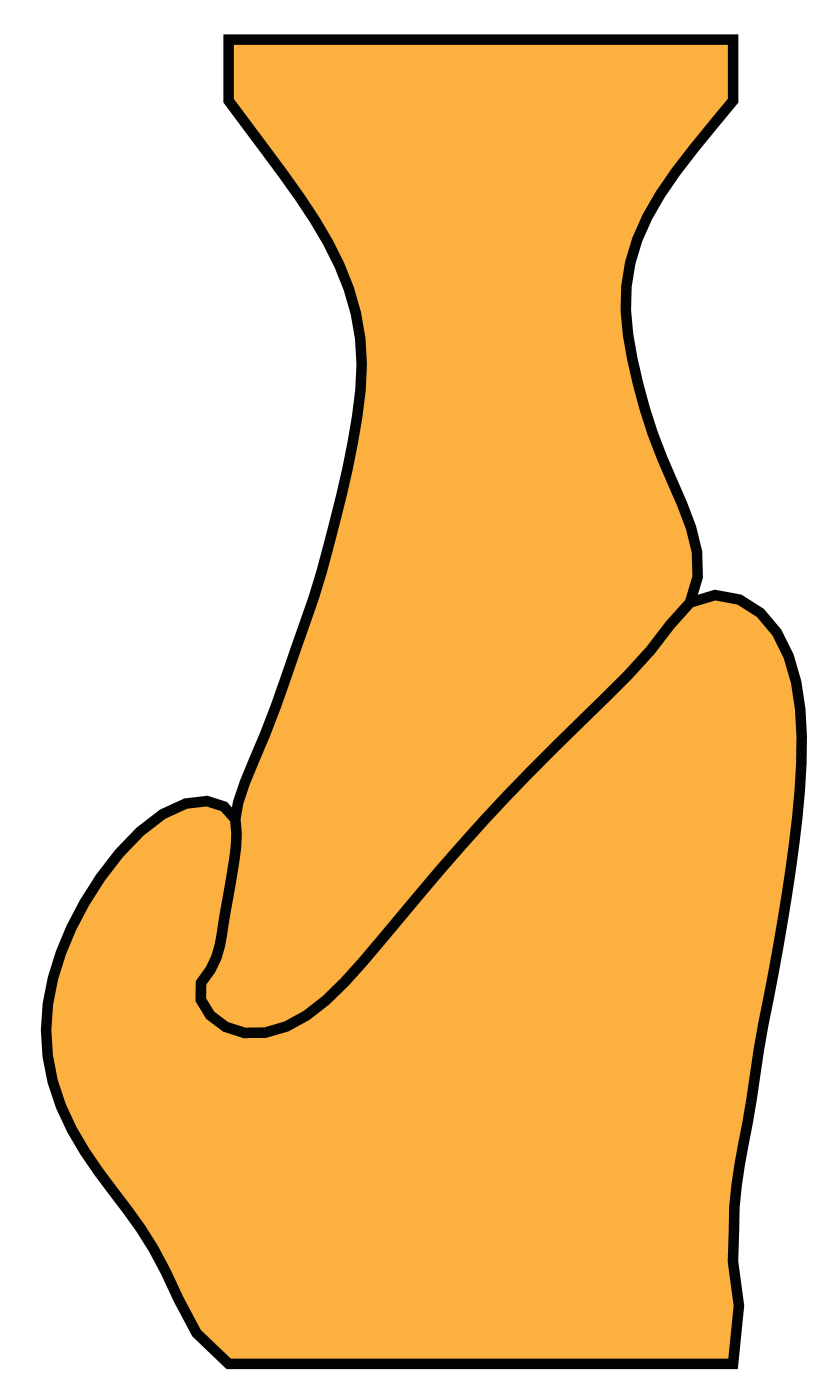
Initial stress distribution.

Optimized stress distribution.

(Tozoni et al., 2021).

Figure 8. Static: Interlocking. Result of shape optimization to minimize the $L^{8}$ norm of stress.

Our framework supports contact and transient friction forces between objects without requiring explicit definition of contact pairs. We borrow the experimental setup used in (Tozoni et al., 2021): we optimize the shape of two interlocking 2D parts (Figure 8) to minimize the $L^{8}$ norm of the stress (30). The bottom part is fixed and a force pointing down-right is applied to the top. Figure 8 shows how the shape changes to reduce the maximum stress from $\qty{3.2}{}$ to $\qty{0.29}{}$.

Note that unlike (Tozoni et al., 2021), our contact model does not support overlapping boundary nodes, which are used in (Tozoni et al., 2021) to keep the contact over the optimization. To mimic this behaviour in our setting, we create small displacements on the overlapped boundary nodes along the normal directions as the initial guess for the forward simulation, so that each object is shrinked by a tiny amount and there is no overlap in the initial guess.

We note that our result is expected to be different from (Tozoni et al., 2021), as the contact models are different and the solutions of these problems are in general not unique. Despite their differences, we observe in both cases a reduction in maximal stress of similar magnitude (around 10 times reduction).

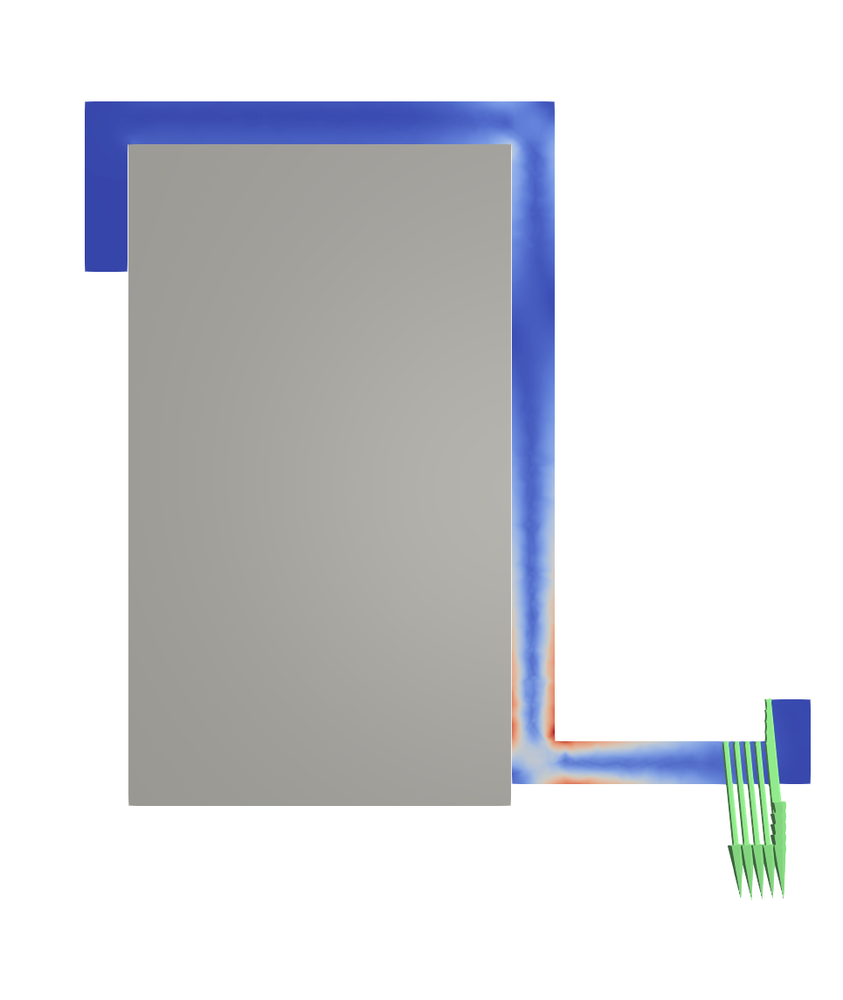
Initial stress distribution.

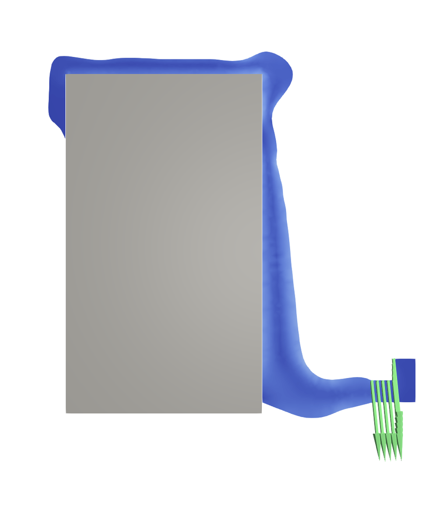
Optimized stress distribution.

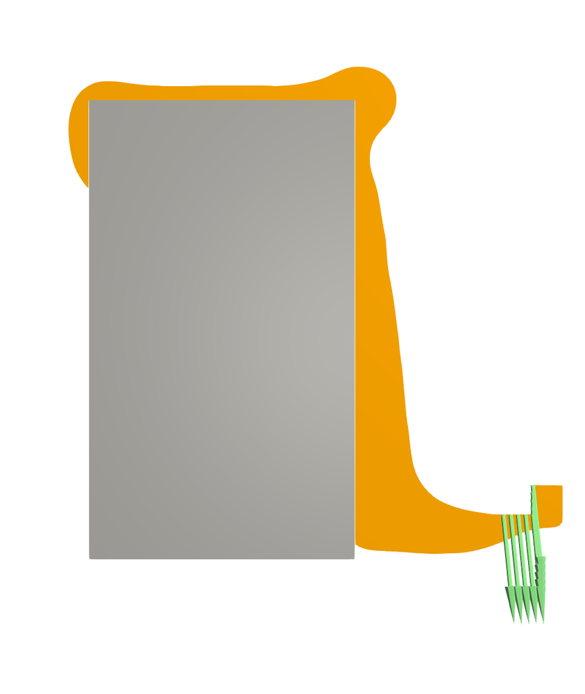
Optimization result from (Tozoni et al., 2021)

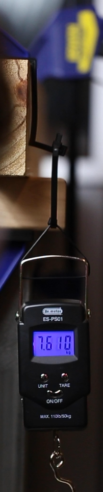
Figure 9. Static: 2D Hook. Shape optimization of a hook to reduce stress concentration (left). Fabricated results with maximum load before failure (right).

Static: 2D Hook

To physically validate our shape optimization results we reproduce the experiment in (Tozoni et al., 2021, Figure 21), where a hook is optimized to minimize the maximum stress (30) when a load is applied to one of its ends (Figure 9). The grey block is fixed with zero Dirichlet conditions on all nodes. We physically validate that the optimized shape is able to withstand a load of over 3$\times$ the unoptimized shape before breaking (Figure 9). The hook has been fabricated using an Ultimaker 3 3D printer, using black PLA plastic. Despite the different contact model, the result is quite similar to the one presented in (Tozoni et al., 2021): our approach has the advantage of not requiring manual specification of the contact surfaces.

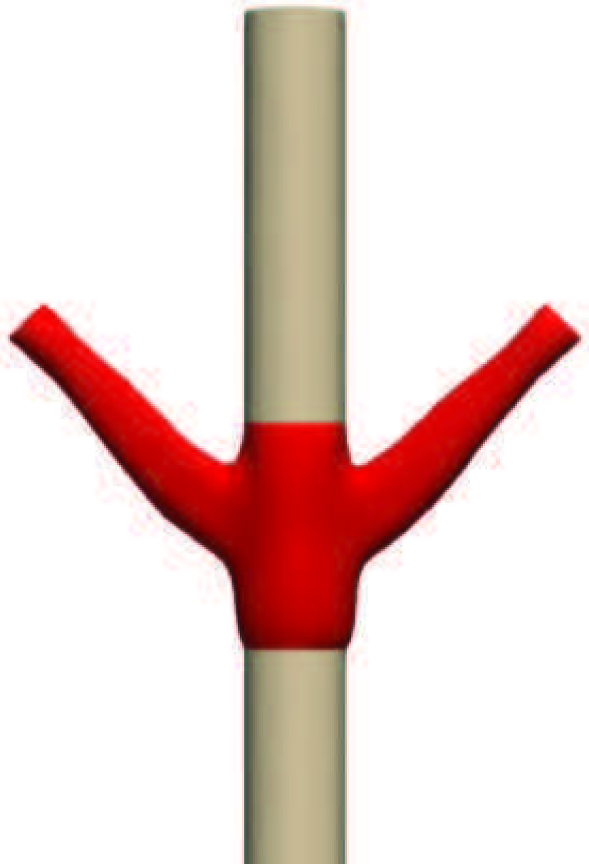
Initial configuration.

Optimized configuration.

(Tozoni et al., 2021)

Figure 10. Static: 3D Hanger. Result of shape optimization of a hanger to reduce stress concentration.

Static: 3D Hanger

We also reproduce the experiment (Tozoni et al., 2021, Figure 29): a coat hanger is composed of two cylinders and a hanger keeping the together. The shape of the hanger is optimized to minimize the maximum internal stress (30) when two loads are applied on its arms (Figure 10). The maximal stress is reduced from $\qty{89.93}{}$ to $\qty{25.74}{}$. When comparing with (Tozoni et al., 2021), we observe a similar optimized shape and an equivalent stress reduction rate (around 3 times).

Transient: Bouncing ball

Initial shape.

Optimized shape.

Iteration 20.

Iteration 50.

Iteration 70.

Figure 11. Transient: Bouncing ball. The result of the shape optimization (blue surface) matches the desired trajectory (wire-frame).

As a demonstration of shape optimization in a transient setting, we run a forward non-linear simulation of a ball bouncing on a plane and use its trajectory as the optimization goal (32). We then deform the initial shape into an ellipse and try to recover the original shape (Figure 11).

Problem setup.

Initial stress distribution at the frame of contact.

Optimized stress distribution at the frame of contact.

Figure 12. Transient: Sliding Ball. Result of shape optimization to reduce stress.

Transient: Shock Protection

We optimize the shape of a shock-protecting microstructure from (Shan et al., 2015) so that the stress (30) of the load being dropped onto the microstructure is minimized. To accelerate convergence, we adopt a low-parametric shape representation from (Panetta et al., 2015). In Figure 13, the maximal stress is reduced from $\qty{32}{}$ to $\qty{12}{}$. This example involves complex self-contact inside the microstructure. Unlike penalty-based contact, our method is intersection-free regardless of the contact parameters, so able to produce plausible results with the same configuration even though the thickness of beams inside the microstructure changes drastically in the optimization.

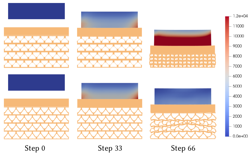
Figure 13. Transient: Shock Protection. Shape optimization of the shock-protecting microstructure to reduce the stress on the falling load. The stress distribution at different time steps is shown for the initial shape (top) and optimized shape (bottom).

Transient: Sliding Ball

We optimize the shape of a ball sliding down a ramp to minimize the internal stress (30). To avoid trivial solutions, we add a volume constraint to not allow its volume to decrease. Perhaps unsurprisingly, the ball gets flattened on the side it contacts with the ramp as this leads to a major reduction of max stress, from $\qty{38}{}$ to $\qty{14}{}$.

9.3. Initial Conditions

Our formulation supports the optimization of objectives depending on the initial conditions. We show three examples: the first involves an object sliding on a ramp with a complex geometry, the second simulates a game of pool, using bunnies instead of spheres, and the third demonstrates complex contact between tentacles.

Initial trajectory.

Iteration 3.

Iteration 5

. Optimized result

Figure 14. Transient: Puzzle Piece. Optimizing the initial velocity of a bouncing puzzle. Target is shown as a black outline while the trajectory being optimized is blue.

Transient: Puzzle Piece

We synthesise a trajectory using a forward simulation, and we then perturb the initial conditions and try to reconstruct them minimizing (31), with an additional integration over time (Figure 14). The puzzle piece uses a Neo-Hookean material.

Transient: Throw Bunny

We use our solver to optimize the throw (initial velocity) of a bunny to hit and displace a second bunny into the prescribed circle (Figure 1), minimizing (32). This example involves complex contact between the bunnies and the pool table, and also friction forces slowing down the sliding after contact.

Transient: Colliding Tentacles

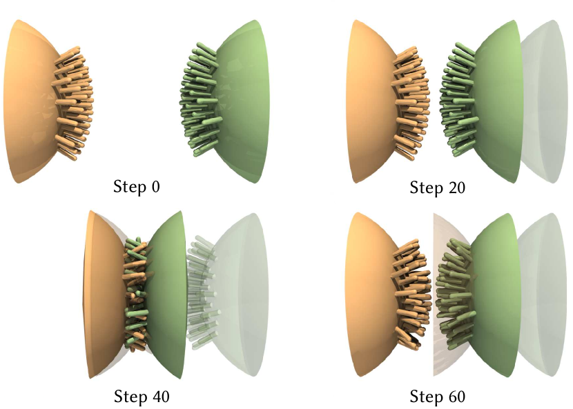
Figure 15. Transient: Colliding Tentacles. We optimize the initial velocity so that the mass trajectory matches the reference simulation. The faded view represents the initial configuration. The optimized simulation matches exactly with the reference simulation.

We optimize the initial velocity of the green object in the scene of two colliding half spheres with tentacles (Figure 15), minimizing the difference of the mass trajectory with respect to a trajectory obtained from a reference simulation (32). Our method manages to resolve the complex contact between the soft tentacles.

9.4. Material Optimization

Next, we look at material optimization problems, where our differentiable simulator is used to estimate the material properties of an object from observations of its displacement.

Initial displacement.

Optimized displacement.

Optimized $E$ pattern.

Optimized $\nu$ pattern.

Figure 16. Static: Sine. Optimized material parameters to obtain a displacement (blue surface) in $y$-direction similar to a sine function for a linear material model (wire-frame).

Static: Sine

We optimize the material of a bar to match the shape of a sine function (wire-frame) when Dirichlet boundary conditions are applied at its ends (31). The rest shape of this bar is a rectangle $[-4,4]\times[-0.3,0.3]$, the left and right surfaces are fixed by Dirichlet boundary condition of $u_{y}=0.7\sin(x+u_{x})$ and $u_{x}=-sign(x)$, and no body force is applied. Figure 16 shows that deformed bar is aligned with a sine function.

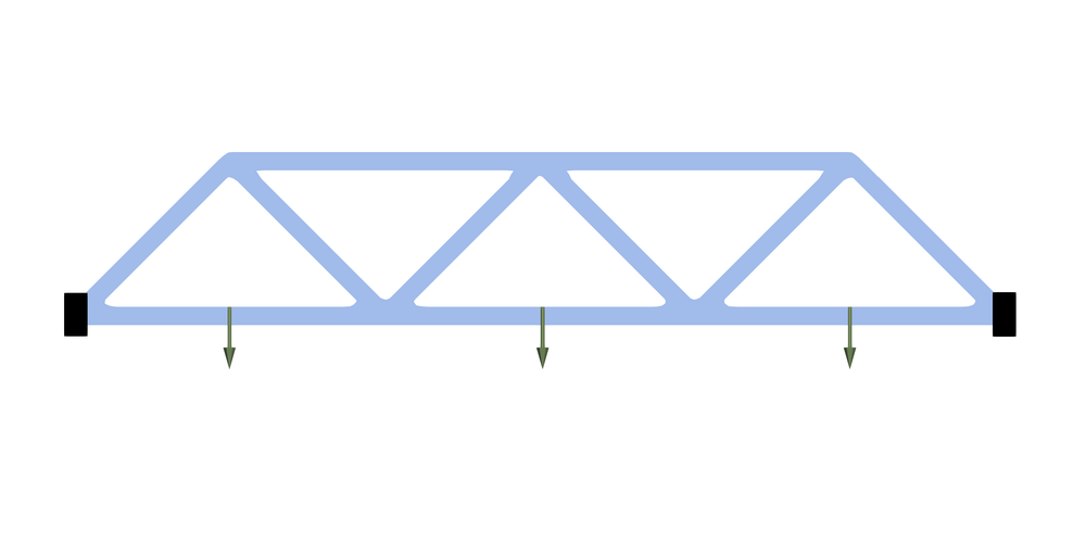
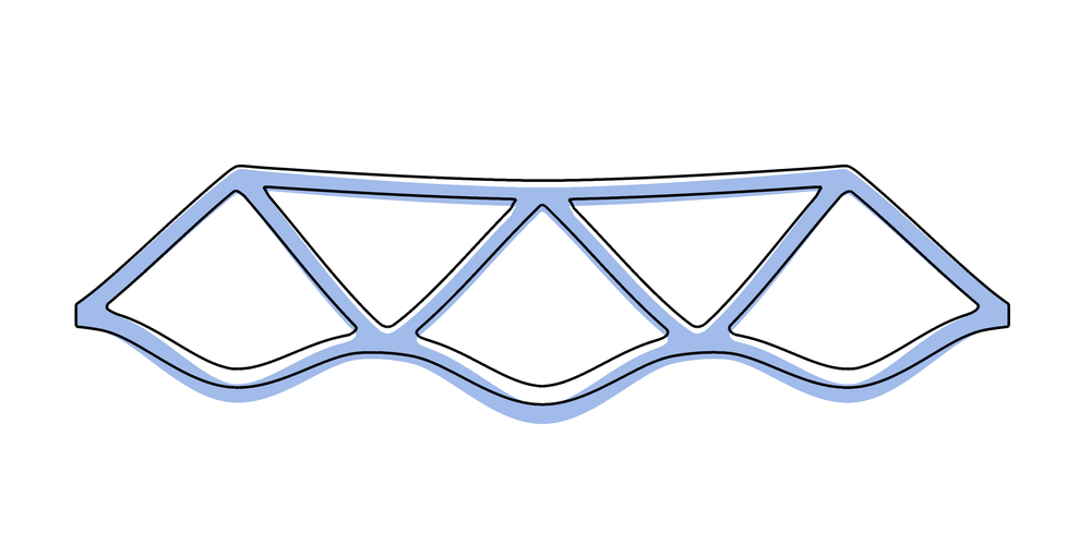
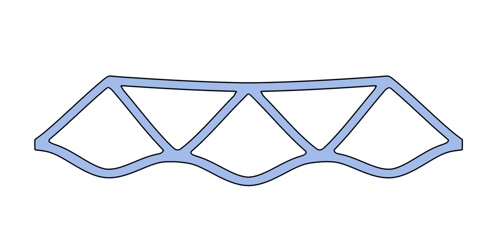
Problem setup.

Initial displacement.

Optimized displacement.

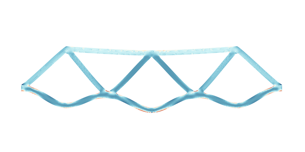
Optimized $E$ pattern.

Optimized $\nu$ pattern.

Figure 17. Static: Bridge. Optimization of the materials of a bridge (blue surface) to match a forward simulation (wire-frame).

Static: Bridge

We assign material parameters $\lambda=160,\mu=80$ to a bridge shape and run a linear forward simulation to obtain the target displacement $u^{\star}$ (Figure 17 in gray), using the same set of boundary conditions as Figure 5. We initialize the optimization using uniform material $\lambda=100,\mu=50$ and minimize (31), successfully recovering $\lambda,\mu$ from $u^{\star}$.

Static: Cube

We set up a physical experiment with a silicon rubber cube compressed by a vise. The deformation is acquired using an HP 3D scanner, and a set of marker points is manually extracted from the scan. We minimize (31) to find the material parameters which produce the observed displacements. We found that the material parameter that leads to the smallest error is $\nu=0.4817$ (Young’s modulus does not affect its deformation in this setting) and the L2 error in markers position is $\qty{3.85e-3}{}$.

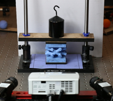
Initial.

Optimized.

Physical Experiment Setup.

Figure 19. Static: Micro-Structure Material optimization of a complex microstructure in a deformed state with contact (blue) to match real data (orange).

Static: Micro-Structure

We repeat the same experiments with the complex geometry of a micro-structure tile from (Panetta et al., 2017). This is a challenging example, as the micro-structure beams come in contact after compression, and physical models without self-contact handling may lead to penetration. The optimization is initialized with $E=\qty{e6}{}$ and $\nu=0.3$ and converges to $E=\qty{2.27e5}{}$ and $\nu=0.348$. Our solver can find material properties $E=\qty{2.27e5}{}$ and $\nu=0.348$ with a L2 error on the markers of $\qty{8.8e-3}{}$.

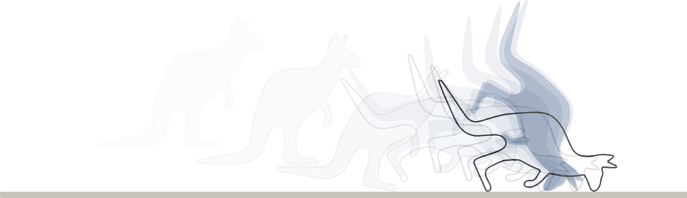
Initial displacement.

Optimized displacement.

Figure 20. Transient: Kangaroo. Non-linear transient simulation of a kangaroo (blue surface) bouncing on a plane to match a target shape (wire-frame).

Transient: Kangaroo

As an example of reconstruction of material parameters from a transient simulation, we run a forward simulation to obtain a transient non-linear target displacement. Then we minimize (31) to reconstruct the material parameters (Figure 20). The initial material parameters are $E=\qty{3e6}{}$ and $\nu=0.5$, and the target material parameters are $E=\qty{e7}{}$ and $\nu=0.3$.

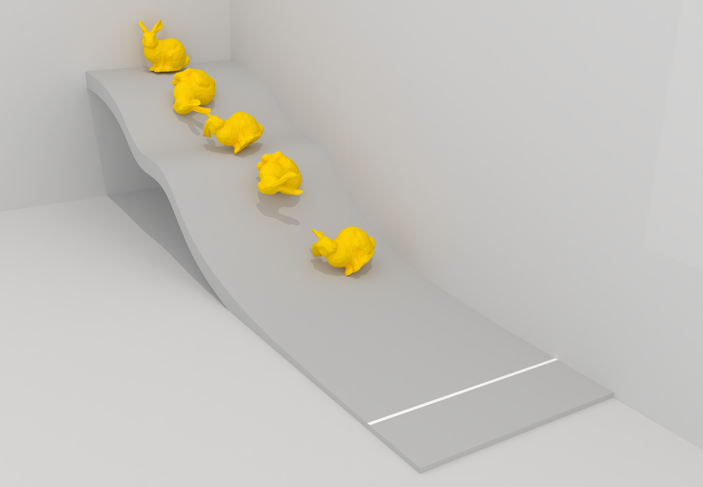
Initial guess.

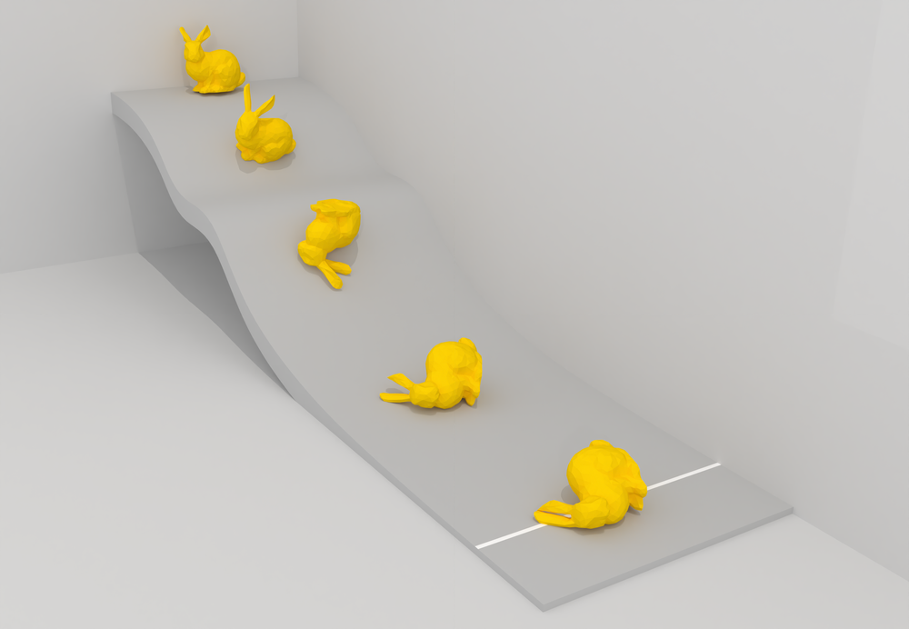
Optimized result.

Figure 21. Transient: Sliding Bunny. Optimize the friction coefficient so that the bunny can reach the white line at $t=2$.

Transient: Sliding Bunny

We use our solver to optimize the friction coefficient to ensure that the bunny is on the white line at time $t=2$. The initial friction coefficient is $\gamma=0.5$, and the optimized friction coefficient is $\gamma=0.0974$ (Figure  21). This example involves complex self-contact and friction of the bunny with the floor.

Initial $E$.

Optimized $E$.

$E=$

Initial $\nu$.

Optimized $\nu$.

$\nu=$

Figure 22. Transient: Bouncing Ball. Material optimization to increase the bouncing height.

Transient: Bouncing Ball

We show that the height of the bounce of a ball can be optimized by changing the material parameters (Figure 22). Initial material parameters for the ball and plank were $E=\qty{e5}{}$, $\nu=0.48$ and $E=\qty{e9}{}$, $\nu=0.48$, respectively and the elasticity model used was NeoHookean. Note that we added a smoothing term to the optimization to increase smoothness in the material parameters.

Transient: Physical Experiment Bouncing Ball

We show that we can optimize for the initial velocity, material parameters, friction coefficient, and damping parameters of a silicone rubber ball bouncing on an incline, using trajectory data from a physical experiment. The real-world dynamics of the ball are captured using a high-speed camera and used to formulate a functional based on (32), which penalizes differences between the observed and simulated barycenter of the ball. The material model used is NeoHookean and we match initial conditions by optimizing for them using the observed barycenters of the ball before it hits the ground.

9.5. Comparisons

Finally, we compare our method with existing methods and finite difference version of PolyFEM (Schneider et al., 2019). Due to stability issues, different time step sizes are chosen for different methods so that no visible artifacts appear in the forward simulations. See Table 5 for statistics.

Table 5. Comparisons. Columns from left to right are examples, methods, degree of freedom of the simulation, time step size, peak memory (), running time of the simulation (), and running time of computing gradients ().

Example	Method	Dofs	dt	Memory	Solve time	Grad time
Armadillo	DiffPD	36699	$3\times 10^{-3}$	1246	37.9	131.2
	GradSim	36699	$1.5\times 10^{-5}$	17164	167.2	N/A
	Ours	36699	$6\times 10^{-3}$	2068	220.6	14.1
Hilbert Cube	DiffPD	4050	$5\times 10^{-2}$	240	1.555	2.12
	GradSim	4050	$5\times 10^{-4}$	1323	11.1	27.7
	Ours	4050	$5\times 10^{-2}$	1599	73.2	1.73
Billiards	DiffPD	978	$2.5\times 10^{-3}$	226	11.3	10.5
	Ours	978	$2.5\times 10^{-3}$	190	66.2	3.1

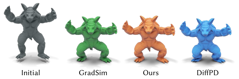
Figure 24. Transient: Armadillo. Simulation of dropping an Armadillo onto the floor.

Transient: Armadillo

We simulate dropping the Armadillo (using the same material parameters) onto a fixed plane (Figure 24) and compute the material derivatives with our method, DiffPD (Du et al., 2021) and GradSim (Jatavallabhula et al., 2021). The results of GradSim and our method are similar, which is expected as both methods are based on a finite element formulation with a similar material model. However, the backward solve of GradSim encounters NAN and fails to compute the gradient, likely due to the instability from its semi-implicit time integration or the non-differentiable contact model (Its contact force is only $C^{0}$). DiffPD creates a result that is different from the two, likely due to the use of a different elastic model.

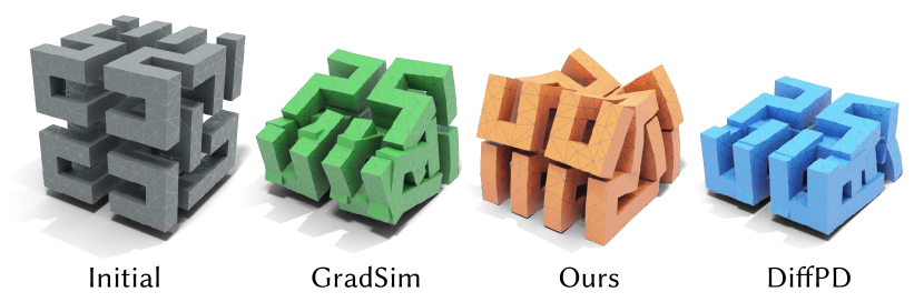
Figure 25. Transient: Hilbert Cube. Simulation of dropping a Hilbert cube onto the floor.

Transient: Hilbert Cube

In this example, we simulate the drop of a Hilbert cube (Figure  25), compute the material derivatives, and compare our method with GradSim and DiffPD. Although GradSim and DiffPD can resolve the planar contact, they do not support self-collision, resulting in visible and physically implausible self-intersections. In contrast, the solution computed by our method has no self-intersections or inverted elements.

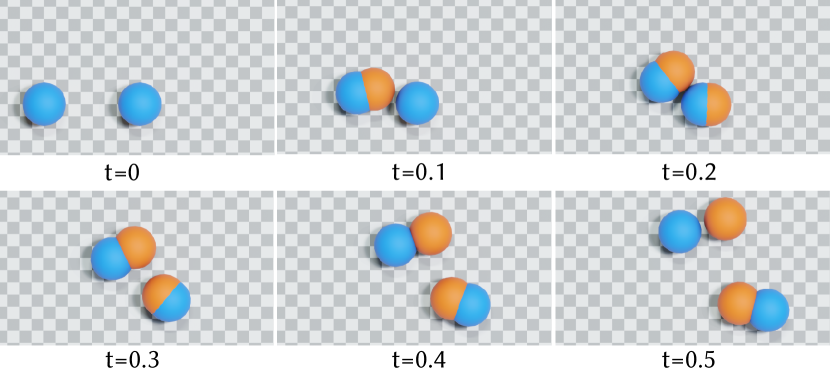
Figure 26. Transient: Billiards. The ball on the left with initial velocity $(\cos(\frac{15}{180}\pi),\sin(\frac{15}{180}\pi))$ hits the ball on the right, simulated with our method (orange) and DiffPD (blue).

Static: Tensile Test

We perform the tensile testing on a bar of size $0.16\unit{}\times 0.08\unit{}\times 0.08\unit{}$, with Poisson’s ratio $\nu=0.3$ and Young’s modulus $E=10^{3}$, using both our method and DiffPD. We refine the meshes used in both methods until the results become stable and show the converged results. Since there is no contact, our method is equivalent to the standard FEM with Neo-Hookean material. Since the material model used in DiffPD is an approximation of the hyper-elastic model designed for high efficiency, there is a noticeable difference between DiffPD and the standard model when the deformation is large (Figure 27). We favor using the Neo-Hookean material model, as we are interested in accurately capturing large physical deformations.

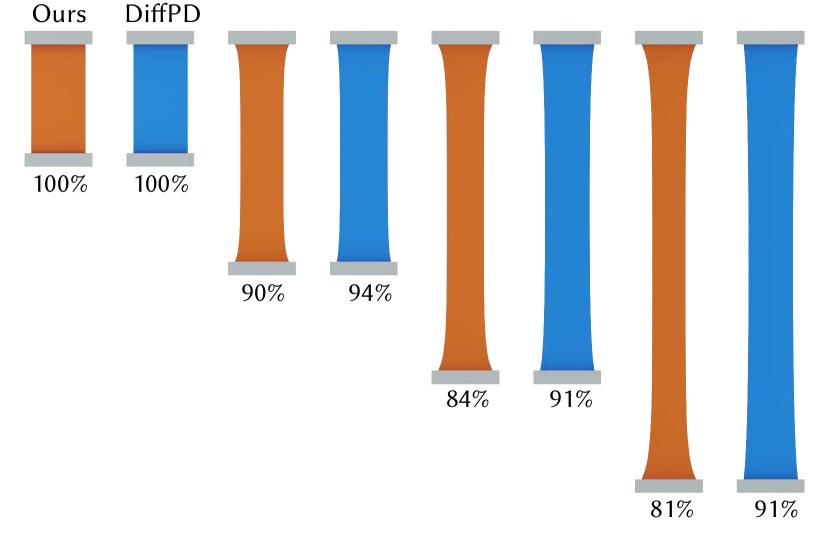
Figure 27. Static: Tensile Test. Stretch a 3D bar up to 300% strain with our method (orange) and DiffPD (blue). The thickness of the deformed bar is shown as a percentage with respect to the initial thickness.

Transient: Billiards

In this example we reproduce the billiards example in  (Du et al., 2021) (Figure 26), and compute the material derivatives. Since GradSim does not support collisions between spheres (or between meshes), we restrict the comparison to DiffPD.

Although the same mesh is used in both methods, there is a significant difference in the contact handling: Our method detects the collision between the discrete meshes, while DiffPD uses the averaged sphere center and radius to detect the collision between spheres. While more efficient, the DiffPD solution is customized for this example, while our approach works on arbitrary geometries. Due to the difference in both the elastic model (Figure 27) and contact handling, the results are different. Our forward simulation is 6 times slower than DiffPD.

Finite Difference

To show the correctness and efficiency of our method, we compute the gradient using the finite difference and compare it with our method. We use the central difference scheme, which requires solving the forward problem for $2n$ times if the parameter dimension is $n$. As a result, the finite difference is at least twice as expensive as the forward solve, while the time of our method is much faster than the forward solve (Table 6).

Table 6. Finite Difference. Columns from left to right are examples, dimension of the design parameters, running time of the simulation (), running time of the adjoint method (), and running time of the finite difference (). The accuracy is the relative error between the finite difference and the adjoint method.

Example	Dim	Solve time	Grad time	FD time	Accuracy
Shock Protection (Figure 13)	24	1273	131.8	63502	$1.12\times 10^{-2}$
Micro-Structure (Figure 19)	2	42.1	0.089	172.1	$2.25\times 10^{-6}$
Sliding Bunny (Figure 21)	1	544.6	1.74	1092	$6.35\times 10^{-10}$

10. Concluding Remarks

We introduced a generic, robust, and accurate framework for PDE-constrained optimization problems involving elastic deformations of multiple objects with contact and friction forces. Our framework supports customizable objective functions and allows for the optimization of functionals involving the geometry of the objects involved, material parameters, contact/friction parameters, and boundary/initial conditions.

There are several limitations in our work. First, our derivation is limited to hyper-elastic and visco-elastic materials. We don’t support simulating shells (cloth), plastic materials, fluid, etc. Second, rigid and articulated objects, which are widely used in robotics, are not supported. Although it can be approximated by very large stiffness in our framework, the simulation is much slower than rigid body simulations. Third, our forward simulation, though robust, is less efficient than previous works like (Du et al., 2021; Jatavallabhula et al., 2021) in simple scenes (Section 9.5).

We believe the benefits of our analytic derivation of the adjoint system (efficiency, generality, guarantee of convergence under refinement) outweigh its downsides (complexity of derivation, difficulty in implementation, and requirement of an explicit FE mesh). We plan to extend our approach to a wider set of PDE-constrained problems and to further optimize it for common use cases in material design and robotics. In particular, we would like to explore the following directions:

1. Add support for periodic boundary conditions, which are required for the design of micro-structure families (Tozoni et al., 2020).

2. Add support for rigid and articulated objects (i.e. allow the material stiffness to be infinite). We plan to incorporate the IPC formulation introduced in (Ferguson et al., 2021) to improve performance in design problems involving rigid objects.

3. Many robotics problems involve the manipulation of plastic objects or interaction with fluids: adding support for additional physical models will widen the applicability of our simulator.

4. We designed our system to provide accurate modeling of elastic, contact, and friction forces, as the majority of PDE-constrained applications require accurate simulations faithfully reproducing the behavior observable in the real works. However, there are applications where this is not necessary, and in these cases, it would be possible to either use simpler elastic models or reduce the accuracy of the collision/friction forces by using proxy geometry. This is commonly done in graphics settings, and it would be interesting to add this option to our system to accelerate its performance.

Appendix A Time-dependent problems

In this section, we show how to compute the derivative and adjoint equation for the time-dependent case. We do this in general form, only assuming that the force terms depend on solution and optimization parameters but not explicitly on time.

Problem setup

We assume all quantities involved in the adjoint equations and shape derivatives for the static case known from the main text. In this appendix, we derive how to update these to obtain the adjoint equation for the time-dependent PDE.

We consider the following time-dependent system, discretized in space.

$$\dot{\mathbf{u}}=\mathbf{v};\;M(\mathbf{q})\dot{\mathbf{v}}=\mathbf{h}(\mathbf{u},\mathbf{q});\;\mathbf{u}(0)=\mathbf{g}^{u}(\mathbf{q});\;\mathbf{v}(0)=\mathbf{g}^{v}(\mathbf{q})$$

where $M(\mathbf{q})$ is the mass matrix, which may also depend on parameters $p$.

We assume that the discretization in time uses a BDF scheme of order $m$:

$$\dot{\mathbf{u}}\approx\frac{1}{\beta\Delta t\,}(\mathbf{u}^{i}+\sum_{j=1}^{\min(i,m)}\alpha^{i}_{j}\mathbf{u}^{i-j}).$$

In general, $\alpha^{i}_{j}$ does not depend on $i$, except at the first $m-1$ steps, when a higher-order scheme needs to be initialized with lower-order steps; more specifically, $\alpha^{i}_{j}$ is $j$-th coefficient of BDFi, for $1\leqslant i<m$, and $j$-th coefficient of BDFm otherwise.

We assume that $\mathbf{h}(\mathbf{u},\mathbf{q})$ does not directly depend on the velocities $\mathbf{v}$; if a dependence on velocities is needed, as we see below, it can be expressed directly in terms of $u$.

The discrete system has the form

(39) $$\begin{split}\mathbf{u}^{i}+\sum_{j=1}^{\min(i,m)}\alpha^{i}_{j}\mathbf{u}^{i-j}&=\beta_{i}\Delta t\,\mathbf{v}^{i},\\ M\bigg{(}\mathbf{v}^{i}+\sum_{j=1}^{\min(i,m)}\alpha^{i}_{j}\mathbf{v}^{i-j}\bigg{)}&=\beta_{i}\Delta t\,\mathbf{h}^{i}(\mathbf{u}^{i},\mathbf{u}^{i-1},\mathbf{q})=\hat{\mathbf{h}}^{i}.\end{split}$$

where $M$ is the mass matrix. This is the form in which the system is solved in (Li et al., 2020).

For time-dependent problems, we consider functionals of the form

$$J(\mathbf{u},\mathbf{q})=\int_{t=0}^{T}J(\mathbf{u},t,\mathbf{q})dt,$$

where $J(\mathbf{u},t,\mathbf{q})$ is a spatial functional, e.g., integral over the solid $\Omega(t)$ or its surface, of some pointwise quantity depending on the solution and/or its derivatives pointwise. In discretized form, this functional is

$$J(\mathbf{u},\mathbf{q})=\sum_{i=0}^{N}w_{i}J_{i}(\mathbf{u}^{i},\mathbf{q})=\sum_{i=0}^{N}\hat{J}^{i},$$

where $w_{i}$ are quadrature weights (e.g., all $\Delta t\,$ in the simplest case), and N is the number of time steps.

Remark on notation

We omit most of the explicit arguments in functions $h$ and $J$ used in the expressions, to make the formulas more readable. The following is implied: $\mathbf{h}(\mathbf{u}^{i},\mathbf{u}^{i-1},\mathbf{q},t_{i})=\mathbf{h}_{i}(\mathbf{u}^{i},\mathbf{u}^{i-1},\mathbf{q})=\mathbf{h}_{i}$ and similarly for $J_{i}$.

Summary

Computing the derivative $d_{\mathbf{q}}J$ requires the following components

• Derivatives $\partial_{\mathbf{u}}J_{i}$, $\partial_{\mathbf{u}}\mathbf{h}_{i}$, $\partial_{\mathbf{q}}J_{i}$ and $\partial_{\mathbf{q}}\mathbf{h}_{i}$. See Sections 7 to 9 in main text for corresponding formulas.

• Derivatives $\partial_{\mathbf{q}}\mathbf{g}^{u}$ and $\partial_{\mathbf{q}}\mathbf{g}^{v}$, derivatives of the initial conditions. See Section 5.4 in main text.

To compute the parametric derivative of $J$, the steps are as follows:

• Solve the forward system (39), and store the resulting solutions $\mathbf{u}^{i},\mathbf{v}^{i}$, $i=0\ldots N$ at every step.

• Initialize adjoint variables $\mathbf{p}_{N},\bm{\nu}_{N}$ from (43) (general BDF: (13)).

• Perform backward time stepping using (41) (general BDF: (12)).

• At every step, evaluate derivative of the mass matrix $d_{\mathbf{q}}M$, if applicable, and use formula (44) (general BDF: (15)) to update $d_{\mathbf{q}}J$.

A.1. Implicit Euler

Discrete Lagrangian

We use the Lagrangian-based approach (Céa’s method) to derive the adjoint equation. The overall idea is to write the Lagrangian $\mathcal{L}$ for the functional $J$ viewing the equations for $\dot{\mathbf{v}}$ and $\dot{\mathbf{u}}$ as constraints with Lagrange multipliers $\mathbf{p}$ and $\bm{\mu}$. For the solution $(\mathbf{u},\mathbf{v})$ for any optimization parameter values, the constraints are satisfied, $d_{\mathbf{q}}J=d_{\mathbf{q}}\mathcal{L}$, as the constraint terms identically vanish. The goal of introducing the adjoint variables is to eliminate the direct dependence of $d_{\mathbf{q}}J$ on the displacement and velocity derivatives: $d_{\mathbf{q}}\mathbf{u}^{i}$ or $d_{\mathbf{q}}\mathbf{v}^{i}$.

To achieve our objective, we expand the derivative $d_{\mathbf{q}}\mathcal{L}$, and isolate the terms multiplying $d_{\mathbf{q}}\mathbf{u}$ and $d_{\mathbf{q}}\mathbf{v}$. By setting the sum of each of these two sets of terms to zero (which corresponds to our adjoint equations), we can find $\mathbf{p}$ and $\bm{\mu}$ so that the derivative of the functional $d_{\mathbf{q}}J$ does not directly depend on $d_{\mathbf{q}}\mathbf{u}^{i}$ or $d_{\mathbf{q}}\mathbf{v}^{i}$.

The time-stepping for implicit Euler/BDF1 has the following simple form:

(40) $$\begin{split}\mathbf{u}^{i}-\mathbf{u}^{i-1}&=\Delta t\,\mathbf{v}^{i},\\ M(\mathbf{v}^{i}-\mathbf{v}^{i-1})&=\Delta t\,\mathbf{h}^{i}=\hat{\mathbf{h}}^{i}.\end{split}$$

We introduce adjoint variables $p_{i}$ and $\mu_{i}$ (we use subscripts for the adjoint variables to indicate the time step, as these are often transposed in the formulas to make the formulas more readable).

In the derivation below, we drop most dependencies on variables, assuming $\hat{J}^{i}=\hat{J}^{i}(\mathbf{u}^{i},\mathbf{q})$, $\mathbf{g}^{u}=\mathbf{g}^{u}(\mathbf{q})$, $\mathbf{g}^{v}=\mathbf{g}^{v}(\mathbf{q})$, $\hat{\mathbf{h}}^{i}=\hat{\mathbf{h}}(\mathbf{u}^{i},\mathbf{u}^{i-1},\mathbf{q})$ and $M=M(\mathbf{q})$.

The Lagrangian $\mathcal{L}$ has the form

$$\mathcal{L} =\sum_{i=0}^{N}\hat{J}^{i}$$ {objective terms}

$$+\mathbf{p}_{0}^{T}(\mathbf{v}^{0}-\mathbf{g}^{v})+\bm{\mu}_{0}^{T}(\mathbf{u}^{0}-\mathbf{g}^{u})$$ {initial condition terms}

$$+\sum_{i=1}^{N}\mathbf{p}^{T}_{i}(M(\mathbf{v}^{i}-\mathbf{v}^{i-1})-\hat{\mathbf{h}}^{i})+\bm{\mu}^{T}_{i}(\mathbf{u}^{i}-\mathbf{u}^{i-1}-\Delta t\,\mathbf{v}^{i}).$$ {PDE terms}

Rearranging terms, and shifting summation index for $\mathbf{u}^{i-1}$,

$$\mathcal{L} =\mathbf{p}_{0}^{T}(\mathbf{v}^{0}-\mathbf{g}^{v})+\bm{\mu}_{0}^{T}(\mathbf{u}^{0}-\mathbf{g}^{u})+\hat{J}^{0}$$

$$+\sum_{i=1}^{N}\hat{J}^{i}+\mathbf{p}^{T}_{i}(M(\mathbf{v}^{i}-\mathbf{v}^{i-1})-\hat{\mathbf{h}}^{i})+\bm{\mu}^{T}_{i}(\mathbf{u}^{i}-\mathbf{u}^{i-1}-\Delta t\,\mathbf{v}^{i})$$

$$=\mathbf{p}_{0}^{T}(\mathbf{v}^{0}-\mathbf{g}^{v})+\bm{\mu}_{0}^{T}(\mathbf{u}^{0}-\mathbf{g}^{u})+\hat{J}^{0}$$

$$+\sum_{i=1}^{N}\hat{J}^{i}+\mathbf{p}^{T}_{i}(M\mathbf{v}^{i}-\hat{\mathbf{h}}^{i})+\bm{\mu}^{T}_{i}(\mathbf{u}^{i}-\Delta t\,\mathbf{v}^{i})-\sum_{i=0}^{N-1}\mathbf{p}^{T}_{i+1}M\mathbf{v}^{i}+\bm{\mu}^{T}_{i+1}\mathbf{u}^{i}.$$

Combining two sums back together and separating $N$-th term from the first, we get

$$\small\begin{split}\mathcal{L}&=\mathbf{p}_{0}^{T}(\mathbf{v}^{0}-\mathbf{g}^{v})+\bm{\mu}_{0}^{T}(\mathbf{u}^{0}-\mathbf{g}^{u})+\hat{J}^{0}-\mathbf{p}^{T}_{1}M\mathbf{v}^{0}-\bm{\mu}^{T}_{1}\mathbf{u}^{0}\\ &+\sum_{i=1}^{N-1}\hat{J}^{i}+\mathbf{p}^{T}_{i}(M\mathbf{v}^{i}-\hat{\mathbf{h}}^{i})+\bm{\mu}^{T}_{i}(\mathbf{u}^{i}-\Delta t\,\mathbf{v}^{i})-\mathbf{p}^{T}_{i+1}M\mathbf{v}^{i}-\bm{\mu}^{T}_{i+1}\mathbf{u}^{i}\\ &+\hat{J}^{N}+\mathbf{p}^{T}_{N}(M\mathbf{v}^{N}-\hat{\mathbf{h}}^{N})+\bm{\mu}^{T}_{N}(\mathbf{u}^{N}-\Delta t\,\mathbf{v}^{N}).\end{split}$$

Collecting $\mathbf{u}^{i}$ and $\mathbf{v}^{i}$ terms:

$$\small\begin{split}\mathcal{L}&=\hat{J}^{0}-\mathbf{p}_{0}^{T}\mathbf{g}^{v}-\bm{\mu}_{0}^{T}\mathbf{g}^{u}+(\mathbf{p}_{0}^{T}-\mathbf{p}^{T}_{1}M)\mathbf{v}^{0}+(\bm{\mu}_{0}^{T}-\bm{\mu}^{T}_{1})\mathbf{u}^{0}\\ &+\sum_{i=1}^{N-1}\hat{J}^{i}-\mathbf{p}^{T}_{i}\hat{\mathbf{h}}^{i}+(\bm{\mu}^{T}_{i}-\bm{\mu}^{T}_{i+1})\mathbf{u}^{i}+((\mathbf{p}^{T}_{i}-\mathbf{p}^{T}_{i+1})M-\bm{\mu}^{T}_{i}\Delta t\,)\mathbf{v}^{i}\\ &+\hat{J}^{N}-\mathbf{p}^{T}_{N}\hat{\mathbf{h}}^{N}+\bm{\mu}^{T}_{N}\mathbf{u}^{N}+(\mathbf{p}^{T}_{N}M-\bm{\mu}^{T}_{N}\Delta t\,)\mathbf{v}^{N}.\end{split}$$

Differentiating with respect to $\mathbf{q}$:

$$\scriptsize\begin{split}d_{\mathbf{q}}\mathcal{L}&=\partial_{\mathbf{q}}\hat{J}^{0}-\mathbf{p}_{0}^{T}\partial_{\mathbf{q}}\mathbf{g}^{v}-\bm{\mu}_{0}^{T}\partial_{\mathbf{q}}\mathbf{g}^{u}-\mathbf{p}^{T}_{1}\partial_{\mathbf{q}}M\mathbf{v}^{0}+(\mathbf{p}_{0}^{T}-\mathbf{p}^{T}_{1}M)d_{\mathbf{q}}\mathbf{v}^{0}+\\ &+(\partial_{\mathbf{u}^{i}}\hat{J}^{0}+\bm{\mu}_{0}^{T}-\bm{\mu}^{T}_{1})d_{\mathbf{q}}\mathbf{u}^{0}+\\ &+\sum_{i=1}^{N-1}\partial_{\mathbf{q}}\hat{J}^{i}-\mathbf{p}^{T}_{i}\partial_{\mathbf{q}}\hat{\mathbf{h}}^{i}+(\mathbf{p}^{T}_{i}-\mathbf{p}^{T}_{i+1})\partial_{\mathbf{q}}M\mathbf{v}^{i}+\\ &+\sum_{i=1}^{N-1}(\bm{\mu}^{T}_{i}-\bm{\mu}^{T}_{i+1}+\partial_{\mathbf{u}^{i}}\hat{J}^{i}-\mathbf{p}^{T}_{i}\partial_{\mathbf{u}^{i}}\hat{\mathbf{h}}^{i})d_{\mathbf{q}}\mathbf{u}^{i}-\mathbf{p}^{T}_{i}\partial_{\mathbf{u}^{i-1}}\hat{\mathbf{h}}^{i}\,d_{\mathbf{q}}\mathbf{u}^{i-1}+\\ &+((\mathbf{p}^{T}_{i}-\mathbf{p}^{T}_{i+1})M-\bm{\mu}^{T}_{i}\Delta t\,)d_{\mathbf{q}}\mathbf{v}^{i}+\\ &+\partial_{\mathbf{q}}\hat{J}^{N}-\mathbf{p}^{T}_{N}\partial_{\mathbf{q}}\hat{\mathbf{h}}^{N}+(\partial_{\mathbf{u}^{i}}\hat{J}^{N}-\mathbf{p}^{T}_{N}\partial_{\mathbf{u}^{N}}\hat{\mathbf{h}}^{N}+\bm{\mu}^{T}_{N})d_{\mathbf{q}}\mathbf{u}^{N}+\\ &-\mathbf{p}^{T}_{N}\partial_{\mathbf{u}^{N-1}}\hat{\mathbf{h}}^{N}d_{\mathbf{q}}\mathbf{u}^{N-1}+(\mathbf{p}^{T}_{N}M-\bm{\mu}^{T}_{N}\Delta t\,)d_{\mathbf{q}}\mathbf{v}^{N}+\mathbf{p}^{T}_{N}\partial_{\mathbf{q}}M\mathbf{v}^{N}.\end{split}$$

Reorganizing to have all terms for each $d_{\mathbf{q}}\mathbf{u}^{i}$ together:

$$\scriptsize\begin{split}d_{\mathbf{q}}\mathcal{L}&=\partial_{\mathbf{q}}\hat{J}^{0}-\mathbf{p}_{0}^{T}\partial_{\mathbf{q}}\mathbf{g}^{v}-\bm{\mu}_{0}^{T}\partial_{\mathbf{q}}\mathbf{g}^{u}-\mathbf{p}^{T}_{1}\partial_{\mathbf{q}}M\mathbf{v}^{0}+(\mathbf{p}_{0}^{T}-\mathbf{p}^{T}_{1}M)d_{\mathbf{q}}\mathbf{v}^{0}+\\ &+(\partial_{\mathbf{u}^{i}}\hat{J}^{0}+\bm{\mu}_{0}^{T}-\bm{\mu}^{T}_{1}-\mathbf{p}^{T}_{1}\partial_{\mathbf{u}^{0}}\hat{\mathbf{h}}^{1})d_{\mathbf{q}}\mathbf{u}^{0}\\ &+\sum_{i=1}^{N-1}\partial_{\mathbf{q}}\hat{J}^{i}-\mathbf{p}^{T}_{i}\partial_{\mathbf{q}}\hat{\mathbf{h}}^{i}+(\mathbf{p}^{T}_{i}-\mathbf{p}^{T}_{i+1})\partial_{\mathbf{q}}M\mathbf{v}^{i}\\ &+\sum_{i=1}^{N-1}(\bm{\mu}^{T}_{i}-\bm{\mu}^{T}_{i+1}+\partial_{\mathbf{u}^{i}}\hat{J}^{i}-\mathbf{p}^{T}_{i}\partial_{\mathbf{u}^{i}}\hat{\mathbf{h}}^{i}-\mathbf{p}^{T}_{i+1}\partial_{\mathbf{u}^{i}}\hat{\mathbf{h}}^{i+1})d_{\mathbf{q}}\mathbf{u}^{i}+\\ &+((\mathbf{p}^{T}_{i}-\mathbf{p}^{T}_{i+1})M-\bm{\mu}^{T}_{i}\Delta t\,)d_{\mathbf{q}}\mathbf{v}^{i}\\ &+\partial_{\mathbf{q}}\hat{J}^{N}-\mathbf{p}^{T}_{N}\partial_{\mathbf{q}}\hat{\mathbf{h}}^{N}+(\partial_{\mathbf{u}^{i}}\hat{J}^{N}-\mathbf{p}^{T}_{N}\partial_{\mathbf{u}^{N}}\hat{\mathbf{h}}^{N}+\bm{\mu}^{T}_{N})d_{\mathbf{q}}\mathbf{u}^{N}+\\ &+(\mathbf{p}^{T}_{N}M-\bm{\mu}^{T}_{N}\Delta t\,)d_{\mathbf{q}}\mathbf{v}^{N}+\mathbf{p}^{T}_{N}\partial_{\mathbf{q}}M\mathbf{v}^{N}.\end{split}$$

Introducing $\bm{\mu}=M^{T}\bm{\nu}$, we obtain the following adjoint equations from the terms multiplying $d_{\mathbf{q}}\mathbf{v}^{i}$ and $d_{\mathbf{q}}\mathbf{u}^{i}$ in the summation:

(41) $$\boxed{\begin{aligned} \mathbf{p}_{i}-\mathbf{p}_{i+1}&=\Delta t\,\bm{\nu}_{i},\\ M^{T}(\bm{\nu}_{i}-\bm{\nu}_{i+1})&=(\partial_{\mathbf{u}^{i}}\hat{\mathbf{h}}^{i})^{T}\mathbf{p}_{i}+(\partial_{\mathbf{u}^{i}}\hat{\mathbf{h}}^{i+1})^{T}\mathbf{p}_{i+1}-(\partial_{\mathbf{u}^{i}}\hat{J}^{i})^{T}.\end{aligned}}$$

For the initial conditions we get from the terms multiplying $d_{\mathbf{q}}\mathbf{v}^{N}$ and $d_{\mathbf{q}}\mathbf{u}^{N}$:

(42) $$\mathbf{p}_{N}=\Delta t\,\bm{\nu}_{N},$$

$$M^{T}\bm{\nu}_{N}=(\partial_{\mathbf{u}^{i}}\hat{\mathbf{h}}^{N})^{T}\mathbf{p}_{N}-(\partial_{\mathbf{u}^{i}}\hat{J}^{N})^{T}.$$

By introducing $\mathbf{p}_{N+1}$ and $\bm{\nu}_{N+1}$, the initial conditions can be simplified as

(43) $$\boxed{\begin{aligned} &\mathbf{p}_{N+1}=0,\\ &\bm{\nu}_{N+1}=0.\end{aligned}}$$

For $\mathbf{p}_{0},\bm{\nu}_{0}$ we have $M^{T}\bm{\nu}_{0}=-(\partial_{\mathbf{u}^{0}}\hat{J}^{0})^{T}+M^{T}\bm{\nu}_{1}+\mathbf{p}^{T}_{1}\partial_{\mathbf{u}^{0}}\hat{\mathbf{h}}^{1}$ and $\mathbf{p}_{0}=M^{T}\mathbf{p}_{1}$.

Finally, the expression for $d_{\mathbf{q}}J$ is obtained by dropping all terms with $d_{\mathbf{q}}\mathbf{v}^{i}$ and $d_{\mathbf{q}}\mathbf{u}^{i}$, as these are set to zero by our choice of equations for the adjoint, and retaining the rest:

(44) $$\boxed{\begin{aligned} d_{\mathbf{q}}J&=\partial_{\mathbf{q}}\hat{J}^{0}-\mathbf{p}_{0}^{T}\partial_{\mathbf{q}}\mathbf{g}^{v}-\bm{\mu}_{0}^{T}\partial_{\mathbf{q}}\mathbf{g}^{u}-\mathbf{p}^{T}_{1}\partial_{\mathbf{q}}M\mathbf{v}^{0},\\ &+\sum_{i=1}^{N}\partial_{\mathbf{q}}\hat{J}^{i}-\mathbf{p}^{T}_{i}\partial_{\mathbf{q}}\hat{\mathbf{h}}^{i}+\Delta t\,\bm{\nu}_{i}^{T}\partial_{\mathbf{q}}M\mathbf{v}^{i}.\end{aligned}}$$

A.2. General BDF time integration

Discrete Lagrangian

For the general case, we split the Lagrangian $\mathcal{L}(\mathbf{u},\mathbf{v},\mathbf{p},\bm{\mu},\mathbf{q})$ into three parts: $J(\mathbf{u},\mathbf{q})$ itself, the part $\mathcal{L}_{c}$ containing the Lagrange multipliers for the time steps $i=1\ldots N$, and the part for initial conditions $\mathcal{L}_{in}$

$$\mathcal{L}(\mathbf{u},\mathbf{v},\mathbf{p},\bm{\mu},\mathbf{q})=J(\mathbf{u},\mathbf{q})+\mathcal{L}_{c}(\mathbf{u},\mathbf{v},\mathbf{p},\bm{\mu},\mathbf{q})+\mathcal{L}_{in}(\mathbf{u}^{0},\mathbf{v}^{0},\mathbf{p}^{0},\bm{\mu}^{0},\mathbf{q}),$$

where

$$\mathcal{L}_{in}=\mathbf{p}_{0}^{T}(\mathbf{v}^{0}-\mathbf{g}^{v})+\bm{\mu}_{0}^{T}(\mathbf{u}^{0}-\mathbf{g}^{u}).$$

We start with $\mathcal{L}_{c}$. Remember that $\mathcal{L}_{c}$ depends on $h^{i}$, which has inputs $x$, $u^{i}$ and $u^{i-1}$ (due to friction):

$$\small\mathcal{L}_{c}=\sum_{i=1}^{N}\mathbf{p}^{T}_{i}M\bigg{(}\mathbf{v}^{i}+\sum_{j=1}^{\min(i,m)}\alpha^{i}_{j}\mathbf{v}^{i-j}-\hat{\mathbf{h}}^{i}\bigg{)}+\bm{\mu}^{T}_{i}\bigg{(}\mathbf{u}^{i}+\sum_{j=1}^{\min(i,m)}\alpha^{i}_{j}\mathbf{u}^{i-j}-\beta_{i}\Delta t\,\mathbf{v}^{i}\bigg{)}.$$

We rearrange the double summations in this expression, so that each term depends only on $\mathbf{u}^{i}$ and $\mathbf{v}^{i}$, as the adjoint equations will be obtained by setting coefficients of $d_{\mathbf{q}}\mathbf{u}^{i}$ and $d_{\mathbf{q}}\mathbf{v}^{i}$ to zero after differentiation.

If we have a sum of the form

$$\sum_{i=1}^{N}\sum_{j=1}^{\min(i,m)}\alpha_{j}^{i}c_{i}^{T}z_{i-j},$$

we can change the summation order: let $r=i-j$,

$$\sum_{i=1}^{N}\sum_{r=\max(0,i-m)}^{i-1}\alpha_{i-r}^{i}c_{i}^{T}z_{r}=\sum_{r=0}^{N-1}\sum_{i=r+1}^{\min(r+m,N)}\alpha_{i-r}^{i}c_{i}^{T}z_{r}=\sum_{r=0}^{N-1}\sum_{j=1}^{\min(m,N-r)}\alpha_{j}^{j+r}c_{r+j}^{T}z_{r},$$

where we introduced back $j=i-r$ in the last equation. Finally, renaming $r$ to $i$, we obtain the form for which each term contains $z_{i}$ only:

(45) $$\small\sum_{i=0}^{N-1}\bigg{(}\sum_{j=1}^{\min(m,N-i)}\alpha_{j}^{i+j}c_{i+j}^{T}\bigg{)}z_{i}.$$

Returning to the Lagrangian, we regroup the terms in $\mathcal{L}$ as:

$$\tiny\mathcal{L}_{c}=\sum_{i=1}^{N}\mathopen{}\mathclose{{}\left(\mathbf{p}^{T}_{i}\mathopen{}\mathclose{{}\left(M\mathbf{v}^{i}-\hat{\mathbf{h}}^{i}}\right)+\bm{\mu}^{T}_{i}\mathopen{}\mathclose{{}\left(\mathbf{u}^{i}-\beta_{i}\Delta t\,\mathbf{v}^{i}}\right)}\right)+\sum_{i=1}^{N}\sum_{j=1}^{\min(i,m)}\mathopen{}\mathclose{{}\left(\mathbf{p}^{T}_{i}M\alpha^{i}_{j}\mathbf{v}^{i-j}+\bm{\mu}^{T}_{i}\alpha^{i}_{j}\mathbf{u}^{i-j}}\right).$$

Using (45), we get

$$\tiny\mathcal{L}_{c}=\sum_{i=1}^{N}\mathopen{}\mathclose{{}\left(\mathbf{p}^{T}_{i}\mathopen{}\mathclose{{}\left(M\mathbf{v}^{i}-\hat{\mathbf{h}}^{i}}\right)+\bm{\mu}^{T}_{i}\mathopen{}\mathclose{{}\left(\mathbf{u}^{i}-\beta_{i}\Delta t\,\mathbf{v}^{i}}\right)}\right)+\sum_{i=0}^{N-1}\sum_{j=1}^{\min(m,N-i)}\mathopen{}\mathclose{{}\left(\mathbf{p}^{T}_{i+j}M\alpha^{i+j}_{j}\mathbf{v}^{i}+\bm{\mu}^{T}_{i+j}\alpha^{i+j}_{j}\mathbf{u}^{i}}\right).$$

Collecting the terms for $\mathbf{u}^{i}$ and $\mathbf{v}^{i}$:

$$\scriptsize\begin{split}\mathcal{L}_{c}&=\\ &\sum_{i=1}^{N-1}-\mathbf{p}^{T}_{i}\hat{\mathbf{h}}^{i}+\mathopen{}\mathclose{{}\left(\mathopen{}\mathclose{{}\left(\mathbf{p}^{T}_{i}+\sum_{j=1}^{\min(m,N-i)}\alpha^{i+j}_{j}\mathbf{p}^{T}_{i+j}}\right)M-\beta_{i}\Delta t\,\bm{\mu}^{T}_{i}}\right)\mathbf{v}^{i}+\\ &+\mathopen{}\mathclose{{}\left(\bm{\mu}^{T}_{i}+\sum_{j=1}^{\min(m,N-i)}\alpha^{i+j}_{j}\bm{\mu}^{T}_{i+j}}\right)\mathbf{u}^{i}+\\ &\sum_{j=1}^{m}\mathbf{p}^{T}_{j}M\alpha^{j}_{j}\mathbf{v}^{0}+\bm{\mu}^{T}_{j}\alpha^{j}_{j}\mathbf{u}^{0}+\\ &-\mathbf{p}^{T}_{N}\hat{\mathbf{h}}^{N}+(\mathbf{p}^{T}_{N}M-\beta_{N}\Delta t\,\bm{\mu}^{T}_{N})\mathbf{v}^{N}+\bm{\mu}^{T}_{N}\mathbf{u}^{N}.\end{split}$$

We split this expression again, into $\mathcal{L}^{mid}_{c}+\mathcal{L}^{0}_{c}+\mathcal{L}^{N}_{c}$, corresponding to three lines of the equation; these terms contribute to the time-dependent adjoint equations and boundary conditions. In this form, it is straightforward to differentiate with respect to $q$:

$$\scriptsize\begin{split}d_{\mathbf{q}}\mathcal{L}_{c}^{mid}&=\\ &\sum_{i=1}^{N-1}-\mathbf{p}^{T}_{i}\partial_{\mathbf{q}}\hat{\mathbf{h}}^{i}+\mathopen{}\mathclose{{}\left(\mathbf{p}^{T}_{i}+\sum_{j=1}^{\min(m,N-i)}\alpha^{i+j}_{j}\mathbf{p}^{T}_{i+j}}\right)d_{\mathbf{q}}M\mathbf{v}^{i}+\\ &\sum_{i=1}^{N-1}\mathopen{}\mathclose{{}\left(\bigg{(}\mathbf{p}^{T}_{i}+\sum_{j=1}^{\min(m,N-i)}\alpha^{i+j}_{j}\mathbf{p}^{T}_{i+j}\bigg{)}M-\beta_{i}\Delta t\,\bm{\mu}^{T}_{i}}\right)d_{\mathbf{q}}\mathbf{v}^{i}+\\ &+\mathopen{}\mathclose{{}\left(\bm{\mu}^{T}_{i}+\sum_{j=1}^{\min(m,N-i)}\alpha^{i+j}_{j}\bm{\mu}^{T}_{i+j}-\mathbf{p}^{T}_{i}\partial_{\mathbf{u}^{i}}\hat{\mathbf{h}}^{i}-\mathbf{p}^{T}_{i+1}\,\partial_{\mathbf{u}^{i}}\hat{\mathbf{h}}^{i+1}}\right)d_{\mathbf{q}}\mathbf{u}^{i}+\\ &-\mathbf{p}^{T}_{1}\,\partial_{\mathbf{u}^{0}}\hat{\mathbf{h}}^{1}\,d_{\mathbf{q}}\mathbf{u}^{0}\\ d_{\mathbf{q}}\mathcal{L}_{c}^{0}&=\sum_{j=1}^{m}\alpha^{j}_{j}\mathopen{}\mathclose{{}\left(\mathbf{p}^{T}_{j}d_{\mathbf{q}}M\mathbf{v}^{0}+\mathbf{p}^{T}_{j}Md_{\mathbf{q}}\mathbf{v}^{0}+\bm{\mu}^{T}_{j}d_{\mathbf{q}}\mathbf{u}^{0}}\right)\\ d_{\mathbf{q}}\mathcal{L}_{c}^{N}&=-\mathbf{p}^{T}_{N}\partial_{\mathbf{q}}\hat{\mathbf{h}}^{N}-\mathbf{p}^{T}_{N}\partial_{\mathbf{u}^{N}}\hat{\mathbf{h}}^{N}d_{\mathbf{q}}\mathbf{u}^{N}+\mathbf{p}^{T}_{N}d_{\mathbf{q}}M\mathbf{v}^{N}+\\ &+(\mathbf{p}^{T}_{N}M-\beta_{N}\Delta t\,\bm{\mu}^{T}_{N})d_{\mathbf{q}}\mathbf{v}^{N}+\bm{\mu}^{T}_{N}d_{\mathbf{q}}\mathbf{u}^{N}.\end{split}$$

Similarly, we split

$$d_{\mathbf{q}}J=\sum_{i=1}^{N-1}\partial_{\mathbf{q}}\hat{J}^{i}+\sum_{i=1}^{N-1}\partial_{\mathbf{u}}\hat{J}^{i}d_{\mathbf{q}}\mathbf{u}^{i}+\big{(}\partial_{\mathbf{q}}\hat{J}^{0}+\partial_{\mathbf{u}}\hat{J}^{0}d_{\mathbf{q}}\mathbf{u}^{0}\big{)}+\big{(}\partial_{\mathbf{q}}\hat{J}^{N}+\partial_{\mathbf{u}}\hat{J}^{N}d_{\mathbf{q}}\mathbf{u}^{N}\big{)}=d_{\mathbf{q}}J^{mid}+d_{\mathbf{q}}J^{0}+d_{\mathbf{q}}J^{N}.$$

Adjoint equations

Equating the coefficients of $d_{\mathbf{q}}\mathbf{u}^{i}$ and $d_{\mathbf{q}}\mathbf{v}^{i}$, $i=1\ldots N-1$ to zero in $d_{\mathbf{q}}\mathcal{L}_{c}^{mid}+d_{\mathbf{q}}J^{mid}$, we obtain the adjoint equations:

(46) $$\scriptsize\begin{split}&M^{T}\bigg{(}\mathbf{p}_{i}+\sum_{j=1}^{\min(m,N-i)}\alpha^{i+j}_{j}\mathbf{p}_{i+j}\bigg{)}=\beta_{i}\Delta t\,\bm{\mu}_{i},\\ &\bm{\mu}_{i}+\sum_{j=1}^{\min(m,N-i)}\alpha^{i+j}_{j}\bm{\mu}_{i+j}=(\partial_{\mathbf{u}^{i}}\hat{\mathbf{h}}^{i})^{T}\mathbf{p}_{i}+(\partial_{\mathbf{u}^{i}}\hat{\mathbf{h}}^{i+1})^{T}\mathbf{p}_{i+1}-(\partial_{\mathbf{u}}\hat{J}^{i})^{T},\end{split}$$

for $i=1\ldots N-1$.

Making a substitution $\bm{\mu}=M^{T}\hat{\bm{\nu}}$, we obtain (12).

We obtain the adjoint equation in time in the form very similar to the forward equations (39). The most important difference is that the integration is ”back in time”, i.e., the finite difference formula for time derivative is applied to $i,\ldots i+m$. This means that the system is integrated backwards, starting with $(\mathbf{p}_{N},\bm{\mu}_{N})$. Second, there is a slight difference in the coefficients of the scheme used. Specifically, the starting iterations do not use the lower-order BDF formulas, rather truncations of the same order BDF formula. At the same time, the end iterations, for small $i$, will use lower order coefficients, even though this is not needed. The reason for preferring this (although this seemingly damages the accuracy of the integration of the adjoint) is consistency with the functional discretization: as this fact is a consequence of deriving the adjoint from the time discretization, if we compute the functional using the same discretization, finite differences for the functional will be closer to the adjoint.

Initial conditions for adjoint

The initial conditions follow from setting coefficients of $d_{\mathbf{q}}\mathbf{u}^{N}$ and $d_{\mathbf{q}}\mathbf{v}^{N}$ to zero in $d_{\mathbf{q}}\mathcal{L}_{c}^{N}d_{\mathbf{q}}J^{N}$, i.e.

$$(\partial_{\mathbf{u}}\hat{J}^{N})^{T}-\partial_{\mathbf{u}}\hat{\mathbf{h}}^{N}\mathbf{p}_{N}+\bm{\mu}_{N}=0;\;M^{T}\mathbf{p}_{N}-\beta_{N}\Delta t\,\bm{\mu}_{N}=0.$$

Substituting $\bm{\mu}=M^{T}\bm{\nu}$, we get

$$(\partial_{\mathbf{u}}\hat{J}^{N})^{T}-\partial_{\mathbf{u}^{N}}\hat{\mathbf{h}}^{N}\mathbf{p}_{N}+M^{T}\bm{\nu}_{N}=0;\;\mathbf{p}_{N}-\beta_{N}\Delta t\,\bm{\nu}_{N}=0,$$

and a linear system for for $\bm{\nu}_{N}$:

$$(\partial_{\mathbf{u}}\hat{J}^{N})^{T}+(M^{T}-\beta_{N}\Delta t\,\partial_{\mathbf{u}^{N}}\hat{\mathbf{h}}^{N})\bm{\nu}_{N}=0.$$

Solving these

(47) $$(M^{T}-\beta_{N}\Delta t\,\partial_{\mathbf{u}^{N}}\hat{\mathbf{h}}^{N})\bm{\nu}_{N}=-(\partial_{\mathbf{u}}\hat{J}^{N})^{T},\;\mathbf{p}_{N}=\beta_{N}\Delta t\,\bm{\nu}_{N}.$$

By introducing $\mathbf{p}_{N+1},\ \bm{\nu}_{N+1}$, the initial condition can be simplified as (13).

Finally, the adjoint equations (12) only allow to solve down to to $i=1$; the equations for $\mathbf{p}_{0},\bm{\mu}_{0}$ are derived from $d_{\mathbf{q}}J^{0}+d_{\mathbf{q}}\mathcal{L}_{in}+d_{\mathbf{q}}\mathcal{L}_{c}^{0}$; adding terms containing $d_{\mathbf{q}}\mathbf{u}^{0}$ and $d_{\mathbf{q}}\mathbf{v}^{0}$, we get:

$$\mathopen{}\mathclose{{}\left(\partial_{\mathbf{u}}\hat{J}^{0}+\bm{\mu}_{0}^{T}+\sum_{j=1}^{m}\alpha^{j}_{j}\bm{\mu}^{T}_{j}-\mathbf{p}_{1}^{T}\partial_{\mathbf{u}^{0}}\hat{\mathbf{h}}^{1}}\right)d_{\mathbf{q}}\mathbf{u}^{0}+\mathopen{}\mathclose{{}\left(\mathbf{p}_{0}^{T}+\sum_{j=1}^{m}\alpha^{j}_{j}\mathbf{p}^{T}_{j}M}\right)d_{\mathbf{q}}\mathbf{v}^{0},$$

which yields direct expressions (14) for $\mathbf{p}_{0}$ and $\bm{\mu}_{0}$, based on $\mathbf{p}_{i},\bm{\mu}_{i}$ for $i=1\ldots m$.

Computing the derivative of $J$ from the forward and adjoint solutions

Finally, once the adjoint variables are obtained, we can compute (15), by collecting all terms not containing $d_{\mathbf{q}}\mathbf{u}^{i}$ and $d_{\mathbf{q}}\mathbf{v}^{i}$.

Partial derivatives $\partial_{\mathbf{q}}\hat{\mathbf{h}},\partial_{\mathbf{u}}\hat{\mathbf{h}}$ and $\partial_{\mathbf{q}}\hat{J}_{i}$, $\partial_{\mathbf{u}}\hat{J}_{i}$ are exactly the same as used in the construction of the system for static adjoint and computation of the functional. The differences, specific to time discretization, are:

• Mass matrix derivative $d_{\mathbf{q}}M$. See Section A.3.

• Partial derivatives of the initial conditions with respect to parameters $\partial_{\mathbf{q}}\mathbf{g}^{v}$ and $\partial_{\mathbf{q}}\mathbf{g}^{u}$, for positions and velocities (See Appendix A.4). Typically, a 3D position and velocity for the whole object (or angular velocity for the object rotating as a rigid body) are used as parameters, so these are trivial to compute.

A.3. Mass matrix derivative

Consider our Mass Matrix as follows:

$$M_{Ds+i,Dt+i}=\sum_{e\in E(s)\cap E(t)}\int_{{\bar{q}}^{e}(\hat{K}_{e})}\rho({\textbf{q}})\,\phi^{\mathrm{loc}_{e}(s)}(x)\,\,\phi^{\mathrm{loc}_{e}(t)}(x)\,\,dx,$$

where $i\in\{1,..,D\}$ and $D$ equals $2$ or $3$ (representing dimension). This means mass matrix $M$ has $D\cdot n$ rows and columns. Here, we use notation to define the local index of a node $\mathrm{loc}_{e}(\ell)$ with respect to elements $e$ containing it.

Then, we can obtain the shape derivative with respect to perturbation $\theta$ ($x^{\epsilon}=x+\epsilon\theta(x)$) by computing the Gateaux Derivative below for each element:

$$\partial_{q}M_{Ds+i,Dt+i} =\frac{d}{d\epsilon}\Big{|}_{\epsilon=0}\sum_{e\in E(s)\cap E(t)}\int_{{\bar{q}}^{e}(\hat{K}_{e})^{\epsilon}}\rho({\textbf{q}})\,\phi^{\mathrm{loc}_{e}(s)}(x^{\epsilon})\,\,\phi^{\mathrm{loc}_{e}(t)}(x^{\epsilon})\,\,dx^{\epsilon}$$

$$=\sum_{e\in E(s)\cap E(t)}\int_{{\bar{q}}^{e}(\hat{K}_{e})}\partial_{\mathbf{q}}\rho({\textbf{q}})\,\phi^{\mathrm{loc}_{e}(s)}(x)\,\,\phi^{\mathrm{loc}_{e}(t)}(x)+$$

$$+\rho({\textbf{q}})\,\phi^{\mathrm{loc}_{e}(s)}(x)\,\,\phi^{\mathrm{loc}_{e}(t)}(x)\,\,\nabla\cdot\theta(x)\,\,dx$$

$$=\sum_{e\in E(s)\cap E(t)}\sum_{l\in\mathrm{Loc}_{e}}\int_{{\bar{q}}^{e}(\hat{K}_{e})}\partial_{\mathbf{q}}\rho({\textbf{q}})\,\phi^{\mathrm{loc}_{e}(s)}(x)\,\,\phi^{\mathrm{loc}_{e}(t)}(x)\,+$$

$$+\,\rho({\textbf{q}})\,\phi^{\mathrm{loc}_{e}(s)}\,\,\phi^{\mathrm{loc}_{e}(t)}\,\,\nabla\xi^{l}\,\,dx\cdot\theta^{l}.$$

A.4. Initial condition derivatives

We need to compute partial derivatives of the initial conditions with respect to optimization parameters $\mathbf{q}$, $\partial_{\mathbf{q}}\mathbf{g}^{v}$ and $\partial_{\mathbf{q}}\mathbf{g}^{u}$, for positions and velocities. Notice that both $\partial_{\mathbf{q}}\mathbf{g}^{v}$ and $\partial_{\mathbf{q}}\mathbf{g}^{u}$ are discrete vector fields on domain $\Omega_{\mathbf{{\bar{q}}}}$. Consider we have one vector value $\mathbf{q}^{m}$ per node of the domain.

If $(\mathbf{g}^{v})_{s}=\mathbf{q}^{m}$, where $(\mathbf{g}^{v})_{s}$ is initial condition at node $s$, the derivative with respect to $q_{m}$ is simply the identity matrix ($\partial_{\mathbf{q}^{m}}(\mathbf{g}^{v})_{s}=I$). At the same time, it is the zero matrix w.r.t. any other $q^{m^{*}}$, with $m^{*}\neq m$. Same thing goes for $\mathbf{g}^{u}$.

Appendix B Parametric derivatives of forces

In this section, we derive general expressions for gradient-dependent volume forces.

In a general form, the contribution to the PDE can be written as

$$\mathcal{H}^{v}(u,w,Q)=\int_{\Omega_{\bar{q}}}f^{v}((\nabla u(x),q(x)):\nabla w\,dx.$$

B.1. Gradient-dependent volume forces

Shape derivatives

we omit the dependence on $\mathbf{q}$, and use $\nabla f$ to denote $\partial_{\nabla u}f$.

Define $\Omega_{\epsilon}=\Omega_{{\mathbf{{\bar{q}}}}+\bm{\theta}\epsilon}$, $\Omega=\Omega_{{\mathbf{{\bar{q}}}}}$ and $x^{\epsilon}=x+\epsilon\theta$. Let $u^{\epsilon}$ be the solution on domain $\Omega_{\epsilon}$. Then computing the Gâteaux derivative of $\mathcal{H}^{v}$ we get:

(48) $$\small\begin{split}\frac{d}{d\epsilon}\Big{|}_{\epsilon=0}\mathcal{H}^{f}=&\frac{d}{d\epsilon}\Big{|}_{\epsilon=0}\int_{\Omega_{\epsilon}}f(\nabla_{x^{\epsilon}}u^{\epsilon}):\nabla_{x^{\epsilon}}w^{\epsilon}\,\,dx^{\epsilon}\\ =&\frac{d}{d\epsilon}\Big{|}_{\epsilon=0}\int_{\Omega}f((\nabla u)F_{\epsilon}^{-1}):(\nabla w)F_{\epsilon}^{-1}\,\,\det F_{\epsilon}\,\,dx\\ =&\int_{\Omega}\frac{d}{d\epsilon}\Big{|}_{\epsilon=0}\mathopen{}\mathclose{{}\left(f((\nabla u)F_{\epsilon}^{-1})F_{\epsilon}^{-T}:\nabla w\,\,\det F_{\epsilon}}\right)\,\,dx\\ =&\int_{\Omega}-f(\nabla u)\nabla\theta^{T}:\nabla w+\boxed{(\nabla f(\nabla u):\nabla\delta u):\nabla w}+\\ -&(\nabla f(\nabla u):(\nabla u\nabla\theta)):\nabla w+\mathopen{}\mathclose{{}\left(f(\nabla u):\nabla w\,}\right)\nabla\cdot\theta\,\,dx.\end{split}$$

Thus we have for the shape derivative contribution:

$$\scriptsize\boxed{B^{f}(\theta,p)=\int_{\Omega}-f(\nabla u)\nabla\theta^{T}:\nabla p-(\nabla f(\nabla u):(\nabla u\nabla\theta)):\nabla p+\mathopen{}\mathclose{{}\left(f(\nabla u):\nabla p\,}\right)\nabla\cdot\theta\,\,dx.}$$

$B^{f}(\theta,p)$ is linear in $\theta$ and $p$, and we convert it to a matrix form by substituting basis functions for $\theta$ and $p$:

$$[ B^{f}]_{Da+i,Db+j}=\sum_{e\in E(a)\cap E(b)}\,\sum_{k,l\in{1..D}}\delta_{i,j}\int_{{\bar{q}}^{e}(\hat{K}_{e})}-[\nabla\xi^{\mathrm{loc}_{e}(b)}]_{k}\,f_{kl}\,[\nabla\phi^{\mathrm{loc}_{e}(a)}]_{l}\,\,dx\,\,+$$

$$+\sum_{e\in E(a)\cap E(b)}\,\sum_{k,l,m\in{1..D}}\int_{{\bar{q}}^{e}(\hat{K}_{e})}-\nabla f(\nabla u)_{iklm}[\nabla\xi^{\mathrm{loc}_{e}(b)}]_{l}[\nabla u]_{jm}[\nabla\varphi^{\mathrm{loc}_{e}(a)}]_{k}\,\,dx\,\,+$$

$$+\sum_{e\in E(a)\cap E(b)}\,\sum_{k\in{1..D}}\int_{{\bar{q}}^{e}(\hat{K}_{e})}f(\nabla u)_{ik}[\nabla\phi^{\mathrm{loc}_{e}(a)}]_{k}[\nabla\xi^{\mathrm{loc}_{e}(b)}]_{j}\,\,dx.$$

the sum is over elements $e$ containing both $a$ and $b$. Again, we use notation $\mathrm{loc}_{e}(\ell)$ to define the local index of a node with respect to the elements $e$ containing it.

The contribution to the left-hand side of the adjoint equation is

$$\boxed{A^{f}(\psi,p)=\int_{\Omega}(\nabla f(\nabla u):\nabla\psi):\nabla p\,dx,}$$

which is the boxed term from (48), corresponding to $w^{T}\partial_{\mathbf{u}}h\,\delta u$, with replacements $w:=p$ and $\delta u:=\psi$. Discretizing according to our FE basis:

$$[A^{f}]_{Da+i,Db+j} =\sum_{e\in E(a)\cap E(b)}\,\sum_{k,l\in{1..D}}\int_{{\bar{q}}^{e}(\hat{K}_{e})}(\nabla f)_{ikjl}[\nabla\phi^{\mathrm{loc}_{e}(b)}]_{l}[\nabla\phi^{\mathrm{loc}_{e}(a)}]_{k}\,\,dx,$$

where we sum over all elements $\Omega_{e}={\bar{q}}(\hat{K})$, with $\hat{K}$ being the reference element.

Non-shape volumetric parameter derivatives

We assume that the force depends on $q=q(x)$, a function of the point in $\Omega_{\bar{q}}$, defined by its values $\mathbf{q}$ at the same nodes as the solution, and interpolated using the same basis $\phi$.

The perturbed parameter function $q$ is defined as

$$q^{\epsilon}(x)=q(x)+\epsilon\theta(x),$$

where $\theta(x)$ represents the perturabtion, assumed to be given in the same basis as $q$ and solution.

(49) $$\begin{split}\frac{d}{d\epsilon}\Big{|}_{\epsilon=0}\mathcal{H}^{v}=&\frac{d}{dt}\Big{|}_{\epsilon=0}\int_{\Omega_{\epsilon}}f(\nabla u^{\epsilon},q^{\epsilon}):\nabla w^{\epsilon}\,\,dx^{\epsilon}\\ =&\int_{\Omega}(\nabla_{1}f:\nabla\delta u):\nabla w\,+\,(\nabla_{2}f\cdot\frac{d}{d\epsilon}q^{\epsilon}):\nabla w\,\,dx\\ =&\int_{\Omega}\boxed{(\nabla_{1}f:\nabla\delta u):\nabla w}\,+\,(\nabla_{2}f\cdot\theta):\nabla w\,\,dx.\end{split}$$

Thus, the shape derivative contribution is:

$$\boxed{B^{f}(\theta,p)=\int_{\Omega}(\nabla_{2}f\cdot\theta):\nabla p\,\,dx.}$$

Discretizing:

$$[B^{f}]_{D_{s}a+i,D_{s}b+j} =\sum_{e\in E(a)\cap E(b)}\,\sum_{k\in{1..D_{d}}}\int_{{\bar{q}}^{e}(\hat{K}_{e})}[\nabla_{2}f]_{ikj}\xi^{\mathrm{loc}_{e}(b)}[\nabla\phi^{\mathrm{loc}_{e}(a)}]_{k}\,\,dx.$$

The contribution to the left-hand side of the adjoint equation is

$$\boxed{A^{f}(\psi,p)=\int_{\Omega}(\nabla_{1}f:\nabla\psi):\nabla p\,dx,}$$

which is the boxed term from (49), depending on $\delta u$ with replacements $w:=p$ and $\delta u:=\psi$.

Discretizing according to our FE basis

$$[A^{f}]_{D_{s}a+i,D_{s}b+j} =\sum_{e\in E(a)\cap E(b)}\,\sum_{k,l\in{1..D_{d}}}\int_{{\bar{q}}^{e}(\hat{K}_{e})}(\nabla_{1}f)_{ikjl}[\nabla\phi^{\mathrm{loc}_{e}(b)}]_{l}[\nabla\phi^{\mathrm{loc}_{e}(a)}]_{k}\,\,dx.$$

Appendix C General form of objective derivatives

For each objective $J$, the derivations below include vectors $R^{o}$ and $S^{o}$, corresponding to $\partial_{u}J$ and $\partial_{q}J$, which are necessary to compute the adjoint solution and the final shape derivative.

C.1. Objectives depending on gradient of solution and shape

Consider an objective that depends on both the solution of the PDE and the domain :

(50) $$J(\nabla u,\Omega)=\int_{\Omega}j(\nabla u,x)dx.$$

Computing the Gateaux derivative, while considering perturbation of the domain $x^{\epsilon}:=x+\epsilon\theta$:

$$\frac{d}{d\epsilon}\Big{|}_{t=0}J =\frac{d}{d\epsilon}\Big{|}_{\epsilon=0}\int_{\Omega_{\epsilon}}j(\nabla u^{\epsilon},x^{\epsilon})\,\,dx^{\epsilon}$$

$$=\frac{d}{d\epsilon}\Big{|}_{\epsilon=0}\int_{\Omega}j((\nabla u)F_{\epsilon}^{-1},x+\epsilon\theta)\det(F_{\epsilon})\,\,dx$$

$$=\int_{\Omega}\frac{d}{d\epsilon}\Big{|}_{\epsilon=0}\mathopen{}\mathclose{{}\left(j((\nabla u)F_{\epsilon}^{-1},x+\epsilon\theta)\det(F_{\epsilon})}\right)\,\,dx$$

$$=\int_{\Omega}\boxed{\nabla_{1}j:\nabla\delta u}\,-\nabla_{1}j:\nabla u\nabla\theta+\nabla_{2}j\cdot\theta+j(\nabla u,x)\nabla\cdot\theta\,\,dx.$$

We can select the parts not depending on $\delta u$ to be part of $S$:

(51) $$S^{o}(\theta)=\int_{\Omega}-\nabla_{1}j:\nabla u\nabla\theta+\nabla_{2}j\cdot\theta+j(\nabla u,x)\nabla\cdot\theta\,\,dx.$$

Discretizing according to our FE basis:

$$[S^{o}]_{Da+i} =\sum_{e\in E(a)}\,\int_{{\bar{q}}^{e}(\hat{K}_{e})}-(\nabla u^{T})_{ij}\mathopen{}\mathclose{{}\left(\nabla_{1}j}\right)_{jk}[\nabla\xi^{\mathrm{loc}_{e}(a)}]_{k}+$$

$$+\frac{\partial j}{\partial x_{i}}\xi^{\mathrm{loc}_{e}(a)}+j(u,x)[\nabla\xi^{\mathrm{loc}_{e}(a)}]_{i}\,\,dx.$$

And,

(52) $$R^{o}(\psi)=\int_{\Omega}\nabla_{1}j:\nabla\psi\,\,dx,$$

which can be discretized as follows:

$$[R^{o}]_{Da+i} =\sum_{e\in E(a)}\,\int_{{\bar{q}}^{e}(\hat{K}_{e})}(\nabla_{1}j)_{ij}\,\,[\nabla\phi^{\mathrm{loc}_{e}(a)}]_{j}\,\,dx.$$

C.2. Objectives depending on solution and shape

Consider an objective that depends on both the solution of the PDE and the domain:

(53) $$J(u,\Omega)=\int_{\Omega}j(u,x)dx.$$

Computing the Gateaux derivative, while considering perturbation of the domain $x^{\epsilon}:=x+\epsilon\theta$:

$$\frac{d}{d\epsilon}\Big{|}_{\epsilon=0}J =\frac{d}{d\epsilon}\Big{|}_{\epsilon=0}\int_{\Omega_{\epsilon}}j(u^{\epsilon},x^{\epsilon})\,\,dx^{\epsilon}$$

$$=\int_{\Omega}\boxed{\nabla_{1}j\cdot\delta u}+\nabla_{2}j\cdot\theta+j\nabla\cdot\theta\,\,dx.$$

We can select the parts depending on $\delta u$, which will be the rhs of our adjoint PDE (represented by vector $R$), while the remaining part is a term that should be added directly to the shape derivative (vector $S$).

So,

(54) $$S^{o}(\theta)=\int_{\Omega}\nabla_{2}j\cdot\theta+j(u,x)\nabla\cdot\theta\,\,dx.$$

Discretizing according to our FE basis:

$$[S]_{Da+i} =\sum_{e\in E(a)}\,\int_{{\bar{q}}^{e}(\hat{K}_{e})}\frac{\partial j}{\partial x_{i}}\xi^{\mathrm{loc}_{e}(a)}+j(u,x)[\nabla\xi^{\mathrm{loc}_{e}(a)}]_{i}\,\,dx.$$

And,

(55) $$R^{o}(\psi)=\int_{\Omega}\nabla_{1}j\cdot\psi\,\,dx,$$

which can be discretized as follows:

$$[R]_{Da+i} =\sum_{e\in E(a)}\,\int_{{\bar{q}}^{e}(\hat{K}_{e})}\frac{\partial j}{\partial u_{i}}\,\,\phi^{\mathrm{loc}_{e}(a)}\,\,dx.$$

Appendix D Contact and Friction Area Term

In our contact and friction formulas, we use $A_{k}$ as a weight for our forces, which measures the area of our contact pair $k$. In the formulation, it corresponds to the sum of surface areas associated with each primitive. In 3D, it is 1/3 of the sum of areas of incident triangles for vertices and edges, and the area of triangles. For a triangle $T=(t_{0},t_{1},t_{2})$, where $t_{i}$ corresponds to the position of each triangle’s vertex, the corresponding triangle area will be:

$$A_{\Delta}(T)=A_{\Delta}(t_{0},t_{1},t_{2})=\tfrac{1}{2}\|(t_{1}-t_{0})\times(t_{2}-t_{0})\|.$$

If $k$ corresponds to a point-triangle contact pair between point $p$ and triangle $T$, and Incid(p) has the incident triangles of $p$, we have:

$$A_{k}=\sum_{T\in\text{Incid}(p)}\tfrac{1}{3}A_{\Delta}(T).$$

In this context, $\partial_{\mathbf{{\bar{q}}}}A_{k}$ corresponds to the gradient of the area term, which can be computed as a sum of the $\partial_{\mathbf{{\bar{q}}}}A_{\Delta}$ terms:

$$\partial_{\mathbf{{\bar{q}}}}A_{\Delta}(T)=\frac{(t_{1}-t_{0})\times(t_{2}-t_{0})}{2\|(t_{1}-t_{0})\times(t_{2}-t_{0})\|}\partial_{\mathbf{{\bar{q}}}}((t_{1}-t_{0})\times(t_{2}-t_{0})).$$

Appendix E Friction Derivative Terms

For friction, we have:

$$B^{f}(p,\theta)=\sum_{k}\partial_{\mathbf{{\bar{q}}}}F^{f}_{k}s\theta\cdot p\,A_{k}+F^{f}_{k}\cdot p\,\,\partial_{\mathbf{{\bar{q}}}}A_{k}\,\,A_{k},$$

and

$$A^{f}(\psi,p)=\sum_{k}\partial_{\mathbf{u}}F_{k}\psi\cdot p\,\,A_{k},$$

which reduces to computing the derivative of each $F^{f}_{k}$ term with respect to $x$, $u^{i}$ and $u^{i-1}$.

(56) $$\begin{split}\partial_{x_{\ell}}F^{f}_{k}&=-\gamma_{k_{1},k_{2}}\,\,T_{k}f_{\eta}(\lVert\tau_{k}\rVert)\frac{\tau_{k}}{\lVert\tau_{k}\rVert}\times\\ &\mathopen{}\mathclose{{}\left(\kappa\frac{N_{k}}{\lVert N_{k}\rVert}\cdot(b^{\prime\prime}(\partial_{\mathbf{x^{d}}}d_{k})(\partial_{\mathbf{x^{d}}}d_{k})^{T}+b^{\prime}\partial_{\mathbf{x^{d}}}(\partial_{\mathbf{x^{d}}}d_{k}))\,\,M^{*}}\right)_{\ell}+\\ &-\gamma_{k_{1},k_{2}}\,N_{k}\mathopen{}\mathclose{{}\left(\partial_{\mathbf{x^{p}}}T_{k}\,M^{*}}\right)_{\ell}f_{\eta}(\lVert\tau_{k}\rVert)\frac{\tau_{k}}{\lVert\tau_{k}\rVert}+\\ &-\gamma_{k_{1},k_{2}}\,N_{k}T_{k}\,\frac{\tau_{k}}{\lVert\tau_{k}\rVert}\mathopen{}\mathclose{{}\left(f_{\eta}^{\prime}\frac{\tau_{k}}{\lVert\tau_{k}\rVert}\cdot((\partial_{\mathbf{x^{p}}}T_{k}\,M^{*})_{\ell}^{T}(\mathbf{u}^{i}-\mathbf{u}^{i-1}))}\right)+\\ &-\gamma_{k_{1},k_{2}}\,N_{k}T_{k}f_{\eta}(\lVert\tau_{k}\rVert)\mathopen{}\mathclose{{}\left(\mathopen{}\mathclose{{}\left(\frac{I_{2}}{\lVert\tau_{k}\rVert}-\frac{\tau_{k}\tau_{k}^{T}}{\lVert\tau_{k}\rVert^{3}}}\right)(\partial_{\mathbf{x^{p}}}T_{k}\,M^{*})_{\ell}^{T}(\mathbf{u}^{i}-\mathbf{u}^{i-1})}\right).\end{split}$$

(57) $$\begin{split}\partial_{u^{i}_{\ell}}F^{f}_{k}&=-\gamma_{k_{1},k_{2}}\,N_{k}T_{k}\,\frac{\tau_{k}}{\lVert\tau_{k}\rVert}\mathopen{}\mathclose{{}\left(f_{\eta}^{\prime}\frac{\tau_{k}}{\lVert\tau_{k}\rVert}\cdot\mathopen{}\mathclose{{}\left(T_{k}^{T}}\right)_{\ell}}\right)+\\ &-\gamma_{k_{1},k_{2}}\,N_{k}T_{k}f_{\eta}(\lVert\tau_{k}\rVert)\mathopen{}\mathclose{{}\left(\mathopen{}\mathclose{{}\left(\frac{I_{2}}{\lVert\tau_{k}\rVert}-\frac{\tau_{k}\tau_{k}^{T}}{\lVert\tau_{k}\rVert^{3}}}\right)\mathopen{}\mathclose{{}\left(T_{k}^{T}}\right)_{\ell}}\right).\end{split}$$

(58) $$\begin{split}\partial_{u^{i-1}_{\ell}}F^{f}_{k}&=-\gamma_{k_{1},k_{2}}\,\,T_{k}f_{\eta}(\lVert\tau_{k}\rVert)\frac{\tau_{k}}{\lVert\tau_{k}\rVert}\times\\ &\mathopen{}\mathclose{{}\left(\kappa\frac{N_{k}}{\lVert N_{k}\rVert}\cdot(b^{\prime\prime}\nabla d_{k}\nabla d_{k}^{T}+b^{\prime}\nabla^{2}d_{k})}\right)_{\ell}+\\ &-\gamma_{k_{1},k_{2}}\,N_{k}\mathopen{}\mathclose{{}\left(\partial_{\mathbf{x^{p}}}T_{k}}\right)_{\ell}f_{\eta}(\lVert\tau_{k}\rVert)\frac{\tau_{k}}{\lVert\tau_{k}\rVert}+\\ &-\gamma_{k_{1},k_{2}}\,N_{k}T_{k}\,\frac{\tau_{k}}{\lVert\tau_{k}\rVert}\mathopen{}\mathclose{{}\left(f_{\eta}^{\prime}\frac{\tau_{k}}{\lVert\tau_{k}\rVert}\cdot\mathopen{}\mathclose{{}\left(\partial_{\mathbf{x^{p}}}T_{k}}\right)_{\ell}^{T}(\mathbf{u}^{i}-\mathbf{u}^{i-1}))}\right)+\\ &-\gamma_{k_{1},k_{2}}\,N_{k}T_{k}f_{\eta}(\lVert\tau_{k}\rVert)\mathopen{}\mathclose{{}\left(\mathopen{}\mathclose{{}\left(\frac{I_{2}}{\lVert\tau_{k}\rVert}-\frac{\tau_{k}\tau_{k}^{T}}{\lVert\tau_{k}\rVert^{3}}}\right)\mathopen{}\mathclose{{}\left(\partial_{\mathbf{x^{p}}}T_{k}}\right)_{\ell}^{T}(\mathbf{u}^{i}-\mathbf{u}^{i-1})}\right).\end{split}$$

Appendix F Regularization Derivatives

Scale-invariant smoothing

The regularization in (37) is used for shape optimization, when the optimization parameter is $q_{m}=v_{i}$, a vertex of the shape. That said, the derivative with respect to each vertex $v_{i}$ is:

$$\partial_{v_{i}}J^{\text{smooth}} =p\|s_{i}\|^{p-2}s_{i}^{T}(\partial_{v_{i}}s_{i})+\sum_{j\in N(i)\cap B}p\|s_{j}\|^{p-2}s_{j}^{T}(\partial_{v_{i}}s_{j}).$$

And we have that

$$\partial_{v_{i}}s_{i}=\frac{|N(i)\cap B|I}{\sum_{j\in N(i)\cap B}\|v_{i}-v_{j}\|}-\frac{\mathopen{}\mathclose{{}\left(\sum_{j\in N(i)\cap B}\frac{v_{i}-v_{j}}{\|v_{i}-v_{j}\|}}\right)\mathopen{}\mathclose{{}\left(\sum_{j\in N(i)\cap B}(v_{i}-v_{j})}\right)^{T}}{\mathopen{}\mathclose{{}\left(\sum_{j\in N(i)\cap B}\|v_{i}-v_{j}\|}\right)^{2}}.$$

And, for $\partial_{v_{i}}s_{j}$, where $v_{i}$ is one of the neighbors of $v_{j}$:

$$\partial_{v_{i}}s_{j}=-\frac{I}{\sum_{k\in N(j)\cap B}\|v_{j}-v_{k}\|}+\frac{\mathopen{}\mathclose{{}\left(\frac{v_{j}-v_{i}}{\|v_{j}-v_{i}\|}}\right)\mathopen{}\mathclose{{}\left(\sum_{k\in N(j)\cap B}(v_{j}-v_{k})}\right)^{T}}{\mathopen{}\mathclose{{}\left(\sum_{k\in N(j)\cap B}\|v_{j}-v_{k}\|}\right)^{2}}.$$

Material parameter spatial smoothing

For derivatives of (38) with respect to material parameters $\lambda_{i},\mu_{i}$ we have

$$\partial_{\lambda_{i}}J^{\lambda,\mu\ \text{smooth}}=2\sum_{t^{\prime}\in Adj(t_{i})}\mathopen{}\mathclose{{}\left(\frac{\lambda_{t_{i}}}{\lambda_{t^{\prime}}}-1}\right)+\mathopen{}\mathclose{{}\left(1-\frac{\lambda_{t^{\prime}}}{\lambda_{t_{i}}}}\right)\frac{\lambda_{t^{\prime}}}{\lambda_{t_{i}}^{2}},$$

and

$$\partial_{\mu_{i}}J^{\lambda,\mu\ \text{smooth}}=2\sum_{t^{\prime}\in Adj(t_{i})}\mathopen{}\mathclose{{}\left(\frac{\mu_{t_{i}}}{\mu_{t^{\prime}}}-1}\right)+\mathopen{}\mathclose{{}\left(1-\frac{\mu_{t^{\prime}}}{\mu_{t_{i}}}}\right)\frac{\mu_{t^{\prime}}}{\mu_{t_{i}}^{2}}.$$

References

- (1)
- Alappat et al. (2020) Christie Alappat, Achim Basermann, Alan R. Bishop, Holger Fehske, Georg Hager, Olaf Schenk, Jonas Thies, and Gerhard Wellein. 2020. A Recursive Algebraic Coloring Technique for Hardware-Efficient Symmetric Sparse Matrix-Vector Multiplication. ACM Trans. Parallel Comput. 7, 3, Article 19 (June 2020), 37 pages. https://doi.org/10.1145/3399732
- Alnaes et al. (2015) M. S. Alnaes, J. Blechta, J. Hake, A. Johansson, B. Kehlet, A. Logg, C. Richardson, J. Ring, M. E. Rognes, and G. N. Wells. 2015. The FEniCS Project Version 1.5. Archive of Numerical Software 3 (2015). https://doi.org/10.11588/ans.2015.100.20553
- Bächer et al. (2021) Moritz Bächer, Espen Knoop, and Christian Schumacher. 2021. Design and Control of Soft Robots Using Differentiable Simulation. Current Robotics Reports (2021), 1–11.
- Baque et al. (2018) Pierre Baque, Edoardo Remelli, François Fleuret, and Pascal Fua. 2018. Geodesic convolutional shape optimization. In International Conference on Machine Learning. PMLR, 472–481.
- Belytschko et al. (2000) Ted Belytschko, Wing Kam Liu, and Brian Moran. 2000. Nonlinear Finite Elements for Continua and Structures. John Wiley & Sons, Ltd.
- Beremlijski et al. (2014) P. Beremlijski, J. Haslinger, J. Outrata, and R. Pathó. 2014. Shape Optimization in Contact Problems with Coulomb Friction and a Solution-Dependent Friction Coefficient. SIAM Journal on Control and Optimization 52, 5 (Jan. 2014), 3371–3400. https://doi.org/10.1137/130948070
- Bern et al. (2019) James Bern, Pol Banzet, Roi Poranne, and Stelian Coros. 2019. Trajectory Optimization for Cable-Driven Soft Robot Locomotion. In Robotics: Science and Systems XV, Vol. 1. Robotics: Science and Systems Foundation. https://doi.org/10.15607/rss.2019.xv.052
- Bern et al. (2020) James M. Bern, Yannick Schnider, Pol Banzet, Nitish Kumar, and Stelian Coros. 2020. Soft Robot Control With a Learned Differentiable Model. In 2020 3rd IEEE International Conference on Soft Robotics (RoboSoft). IEEE, 417–423. https://doi.org/10.1109/robosoft48309.2020.9116011
- Bollhöfer et al. (2019) Matthias Bollhöfer, Aryan Eftekhari, Simon Scheidegger, and Olaf Schenk. 2019. Large-scale Sparse Inverse Covariance Matrix Estimation. SIAM Journal on Scientific Computing 41, 1 (2019), A380–A401. https://doi.org/10.1137/17M1147615 arXiv:https://doi.org/10.1137/17M1147615
- Bollhöfer et al. (2020) Matthias Bollhöfer, Olaf Schenk, Radim Janalik, Steve Hamm, and Kiran Gullapalli. 2020. State-of-the-Art Sparse Direct Solvers. (2020), 3–33. https://doi.org/10.1007/978-3-030-43736-7_1
- Bridson et al. (2002) Robert Bridson, Ronald Fedkiw, and John Anderson. 2002. Robust Treatment of Collisions, Contact and Friction for Cloth Animation. ACM Trans. on Graph. 21 (05 2002).
- Brogliato (1999) Bernard Brogliato. 1999. Nonsmooth Mechanics. Springer-Verlag.
- Brown et al. (2018) George E. Brown, Matthew Overby, Zahra Forootaninia, and Rahul Narain. 2018. Accurate Dissipative Forces in Optimization Integrators. ACM Trans. Graph. 37, 6, Article 282 (dec 2018), 14 pages. https://doi.org/10.1145/3272127.3275011
- Chang et al. (2016) Michael B Chang, Tomer Ullman, Antonio Torralba, and Joshua B Tenenbaum. 2016. A compositional object-based approach to learning physical dynamics. arXiv preprint arXiv:1612.00341 (2016).
- Chen et al. (2020) Bicheng Chen, Nianfeng Wang, Xianmin Zhang, and Wei Chen. 2020. Design of dielectric elastomer actuators using topology optimization on electrodes. Smart Mater. Struct. 29, 7 (June 2020), 075029. https://doi.org/10.1088/1361-665x/ab8b2d
- Daviet et al. (2011) Gilles Daviet, Florence Bertails-Descoubes, and Laurence Boissieux. 2011. A Hybrid Iterative Solver for Robustly Capturing Coulomb Friction in Hair Dynamics. ACM Trans. on Graph. 30 (12 2011).
- de Vaucorbeil et al. (2019) Alban de Vaucorbeil, Vinh Phu Nguyen, Sina Sinaie, and Jian Ying Wu. 2019. Material point method after 25 years: theory, implementation and applications. Submitted to Advances in Applied Mechanics (2019), 1.
- Desmorat (2007) B. Desmorat. 2007. Structural rigidity optimization with frictionless unilateral contact. International Journal of Solids and Structures 44, 3 (Feb. 2007), 1132–1144. https://doi.org/10.1016/j.ijsolstr.2006.06.010
- Du et al. (2021) Tao Du, Kui Wu, Pingchuan Ma, Sebastien Wah, Andrew Spielberg, Daniela Rus, and Wojciech Matusik. 2021. DiffPD: Differentiable Projective Dynamics. ACM Trans. Graph. 41, 2, Article 13 (nov 2021), 21 pages. https://doi.org/10.1145/3490168
- Eck et al. (2005) Christof Eck, Jiri Jarusek, Miroslav Krbec, Jiri Jarusek, and Miroslav Krbec. 2005. Unilateral Contact Problems : Variational Methods and Existence Theorems. CRC Press. https://doi.org/10.1201/9781420027365
- Ferguson et al. (2020) Zachary Ferguson et al. 2020. IPC Toolkit. https://ipc-sim.github.io/ipc-toolkit/
- Ferguson et al. (2021) Zachary Ferguson, Minchen Li, Teseo Schneider, Francisca Gil-Ureta, Timothy Langlois, Chenfanfu Jiang, Denis Zorin, Danny M. Kaufman, and Daniele Panozzo. 2021. Intersection-free Rigid Body Dynamics. ACM Transactions on Graphics (SIGGRAPH) 40, 4, Article 183 (2021).
- Gavriil et al. (2020) Konstantinos Gavriil, Ruslan Guseinov, Jesús Pérez, Davide Pellis, Paul Henderson, Florian Rist, Helmut Pottmann, and Bernd Bickel. 2020. Computational Design of Cold Bent Glass FaçAdes. ACM Trans. Graph. 39, 6, Article 208 (nov 2020), 16 pages. https://doi.org/10.1145/3414685.3417843
- Geilinger et al. (2020) Moritz Geilinger, David Hahn, Jonas Zehnder, Moritz Bächer, Bernhard Thomaszewski, and Stelian Coros. 2020. ADD: analytically differentiable dynamics for multi-body systems with frictional contact. ACM Transactions on Graphics (TOG) 39, 6 (2020), 1–15.
- Geuzaine and Remacle (2009) Christophe Geuzaine and Jean-François Remacle. 2009. Gmsh: A 3-D finite element mesh generator with built-in pre- and post-processing facilities. Internat. J. Numer. Methods Engrg. 79, 11 (2009), 1309–1331. https://doi.org/10.1002/nme.2579 arXiv:https://onlinelibrary.wiley.com/doi/pdf/10.1002/nme.2579
- Hafner et al. (2019) Christian Hafner, Christian Schumacher, Espen Knoop, Thomas Auzinger, Bernd Bickel, and Moritz Bächer. 2019. X-CAD: Optimizing CAD Models with Extended Finite Elements. ACM Trans. Graph. 38, 6, Article 157 (Nov. 2019), 15 pages. https://doi.org/10.1145/3355089.3356576
- Hahn et al. (2019) David Hahn, Pol Banzet, James M. Bern, and Stelian Coros. 2019. Real2Sim: Visco-Elastic Parameter Estimation from Dynamic Motion. ACM Trans. Graph. 38, 6, Article 236 (Nov. 2019), 13 pages. https://doi.org/10.1145/3355089.3356548
- Harmon et al. (2009) David Harmon, Etienne Vouga, Breannan Smith, Rasmus Tamstorf, and Eitan Grinspun. 2009. Asynchronous contact mnumpageechanics. In ACM Trans. on Graph. (TOG), Vol. 28. ACM.
- Harmon et al. (2008) David Harmon, Etienne Vouga, Rasmus Tamstorf, and Eitan Grinspun. 2008. Robust Treatment of Simultaneous Collisions. SIGGRAPH (ACM Trans. on Graph.) 27, 3 (2008).
- Haslinger et al. (1986) Jaroslav Haslinger, Pekka Neittaanmaki, and Timo Tiihonen. 1986. Shape optimization in contact problems based on penalization of the state inequality. Aplikace matematiky 31, 1 (1986), 54–77. https://eudml.org/doc/15435
- Heiden et al. (2021) Eric Heiden, Miles Macklin, Yashraj S Narang, Dieter Fox, Animesh Garg, and Fabio Ramos. 2021. DiSECt: A Differentiable Simulation Engine for Autonomous Robotic Cutting. In Proceedings of Robotics: Science and Systems. Virtual. https://doi.org/10.15607/RSS.2021.XVII.067
- Heiden et al. (2020) Eric Heiden, David Millard, Erwin Coumans, Yizhou Sheng, and Gaurav S Sukhatme. 2020. NeuralSim: Augmenting Differentiable Simulators with Neural Networks. arXiv preprint arXiv:2011.04217 (2020).
- Herskovits et al. (2000) J. Herskovits, A. Leontiev, G. Dias, and G. Santos. 2000. Contact shape optimization: a bilevel programming approach. Structural and Multidisciplinary Optimization 20, 3 (Nov. 2000), 214–221. https://doi.org/10.1007/s001580050149
- Hoshyari et al. (2019) Shayan Hoshyari, Hongyi Xu, Espen Knoop, Stelian Coros, and Moritz Bächer. 2019. Vibration-minimizing motion retargeting for robotic characters. ACM Trans. Graph. 38, 4 (July 2019), 1–14. https://doi.org/10.1145/3306346.3323034
- Hsu et al. (2022) Jerry Hsu, Nghia Truong, Cem Yuksel, and Kui Wu. 2022. A General Two-Stage Initialization for Sag-Free Deformable Simulations. ACM Trans. Graph. 41, 4, Article 64 (jul 2022), 13 pages. https://doi.org/10.1145/3528223.3530165
- Hu et al. (2019a) Yuanming Hu, Luke Anderson, Tzu-Mao Li, Qi Sun, Nathan Carr, Jonathan Ragan-Kelley, and Fredo Durand. 2019a. DiffTaichi: Differentiable Programming for Physical Simulation. In International Conference on Learning Representations.
- Hu et al. (2019b) Yuanming Hu, Jiancheng Liu, Andrew Spielberg, Joshua B Tenenbaum, William T Freeman, Jiajun Wu, Daniela Rus, and Wojciech Matusik. 2019b. Chainqueen: A real-time differentiable physical simulator for soft robotics. In 2019 International conference on robotics and automation (ICRA). IEEE, 6265–6271.
- Hu et al. (2020) Yixin Hu, Teseo Schneider, Bolun Wang, Denis Zorin, and Daniele Panozzo. 2020. Fast Tetrahedral Meshing in the Wild. ACM Trans. Graph. 39, 4, Article 117 (July 2020), 18 pages. https://doi.org/10.1145/3386569.3392385
- Jatavallabhula et al. (2021) Krishna Murthy Jatavallabhula, Miles Macklin, Florian Golemo, Vikram Voleti, Linda Petrini, Martin Weiss, Breandan Considine, Jerome Parent-Levesque, Kevin Xie, Kenny Erleben, Liam Paull, Florian Shkurti, Derek Nowrouzezahrai, and Sanja Fidler. 2021. gradSim: Differentiable simulation for system identification and visuomotor control. International Conference on Learning Representations (ICLR) (2021). https://openreview.net/forum?id=c_E8kFWfhp0
- Jiang et al. (2020) Zhongshi Jiang, Teseo Schneider, Denis Zorin, and Daniele Panozzo. 2020. Bijective Projection in a Shell. ACM Trans. Graph. 39, 6, Article 247 (nov 2020), 18 pages. https://doi.org/10.1145/3414685.3417769
- Kikuchi and Oden (1988) Noboru Kikuchi and John Tinsley Oden. 1988. Contact Problems in Elasticity: A Study of Variational Inequalities and Finite Element Methods. SIAM Studies in App. and Numer. Math., Vol. 8. Society for Industrial and Applied Mathematics.
- Knupp (2001) Patrick M. Knupp. 2001. Algebraic Mesh Quality Metrics. SIAM Journal on Scientific Computing 23, 1 (2001), 193–218. https://doi.org/10.1137/S1064827500371499 arXiv:https://doi.org/10.1137/S1064827500371499
- Li et al. (2020) Minchen Li, Zachary Ferguson, Teseo Schneider, Timothy Langlois, Denis Zorin, Daniele Panozzo, Chenfanfu Jiang, and Danny M. Kaufman. 2020. Incremental Potential Contact: Intersection- and Inversion-free Large Deformation Dynamics. ACM Transactions on Graphics 39, 4 (2020).
- Li et al. (2023) Minchen Li, Zachary Ferguson, Teseo Schneider, Timothy Langlois, Denis Zorin, Daniele Panozzo, Chenfanfu Jiang, and Danny M. Kaufman. 2023. Convergent Incremental Potential Contact. arXiv:2307.15908 [math.NA]
- Li et al. (2022) Yifei Li, Tao Du, Kui Wu, Jie Xu, and Wojciech Matusik. 2022. DiffCloth: Differentiable Cloth Simulation with Dry Frictional Contact. ACM Trans. Graph. (mar 2022). https://doi.org/10.1145/3527660 Just Accepted.
- Liang et al. (2019) Junbang Liang, Ming Lin, and Vladlen Koltun. 2019. Differentiable cloth simulation for inverse problems. Neural Information Processing Systems (2019).
- Ly et al. (2018) Mickaël Ly, Romain Casati, Florence Bertails-Descoubes, Mélina Skouras, and Laurence Boissieux. 2018. Inverse Elastic Shell Design with Contact and Friction. ACM Trans. Graph. 37, 6, Article 201 (dec 2018), 16 pages. https://doi.org/10.1145/3272127.3275036
- Maloisel et al. (2021) Guirec Maloisel, Espen Knoop, Christian Schumacher, and Moritz Bacher. 2021. Automated Routing of Muscle Fibers for Soft Robots. IEEE Trans. Robot. 37, 3 (June 2021), 996–1008. https://doi.org/10.1109/tro.2020.3043654
- Maury et al. (2017) Aymeric Maury, Grégoire Allaire, and François Jouve. 2017. Shape optimisation with the level set method for contact problems in linearised elasticity. (Jan. 2017). https://hal.archives-ouvertes.fr/hal-01435325
- Mitusch et al. (2019) Sebastian K. Mitusch, Simon W. Funke, and Jørgen S. Dokken. 2019. dolfin-adjoint 2018.1: automated adjoints for FEniCS and Firedrake. Journal of Open Source Software 4, 38 (2019), 1292. https://doi.org/10.21105/joss.01292
- Otaduy et al. (2009) Miguel Otaduy, Rasmus Tamstorf, Denis Steinemann, and Markus Gross. 2009. Implicit Contact Handling for Deformable Objects. Comp. Graph. Forum 28 (04 2009).
- Panetta et al. (2017) Julian Panetta, Abtin Rahimian, and Denis Zorin. 2017. Worst-case stress relief for microstructures. ACM Transactions on Graphics 36, 4 (2017). https://doi.org/10.1145/3072959.3073649
- Panetta et al. (2015) Julian Panetta, Qingnan Zhou, Luigi Malomo, Nico Pietroni, Paolo Cignoni, and Denis Zorin. 2015. Elastic Textures for Additive Fabrication. ACM Trans. Graph. 34, 4, Article 135 (July 2015), 12 pages.
- Qiao et al. (2020) Yi-Ling Qiao, Junbang Liang, Vladlen Koltun, and Ming Lin. 2020. Scalable Differentiable Physics for Learning and Control. In International Conference on Machine Learning. PMLR, 7847–7856.
- Rabinovich et al. (2017) Michael Rabinovich, Roi Poranne, Daniele Panozzo, and Olga Sorkine-Hornung. 2017. Scalable locally injective mappings. ACM Transactions on Graphics (TOG) 36, 4 (2017), 1.
- Rojas et al. (2021) Junior Rojas, Eftychios Sifakis, and Ladislav Kavan. 2021. Differentiable Implicit Soft-Body Physics. arXiv preprint arXiv:2102.05791 (2021).
- Schneider et al. (2019) Teseo Schneider, Jérémie Dumas, Xifeng Gao, Denis Zorin, and Daniele Panozzo. 2019. PolyFEM. https://polyfem.github.io/.
- Schumacher et al. (2020) Christian Schumacher, Espen Knoop, and Moritz Bacher. 2020. Simulation-Ready Characterization of Soft Robotic Materials. IEEE Robot. Autom. Lett. 5, 3 (July 2020), 3775–3782. https://doi.org/10.1109/lra.2020.2982058
- Schumacher et al. (2018) Christian Schumacher, Jonas Zehnder, and Moritz Bächer. 2018. Set-in-Stone: Worst-Case Optimization of Structures Weak in Tension. ACM Trans. Graph. 37, 6, Article 252 (dec 2018), 13 pages. https://doi.org/10.1145/3272127.3275085
- Shan et al. (2015) Sicong Shan, Sung Kang, Jordan Raney, Pai Wang, Lichen Fang, Francisco Candido, Jennifer Lewis, and Katia Bertoldi. 2015. Multistable Architected Materials for Trapping Elastic Strain Energy. Advanced materials (Deerfield Beach, Fla.) 27 (06 2015). https://doi.org/10.1002/adma.201501708
- Sharma and Maute (2018) Ashesh Sharma and Kurt Maute. 2018. Stress-based topology optimization using spatial gradient stabilized XFEM. Structural and Multidisciplinary Optimization 57, 1 (2018), 17–38.
- Skouras et al. (2013) Mélina Skouras, Bernhard Thomaszewski, Stelian Coros, Bernd Bickel, and Markus Gross. 2013. Computational Design of Actuated Deformable Characters. ACM Trans. Graph. 32, 4, Article 82 (jul 2013), 10 pages. https://doi.org/10.1145/2461912.2461979
- Stewart (2001) David E Stewart. 2001. Finite-dimensional contact mechanics. Phil. Trans. R. Soc. Lond. A 359 (2001).
- Stupkiewicz et al. (2010) Stanisław Stupkiewicz, Jakub Lengiewicz, and Jože Korelc. 2010. Sensitivity analysis for frictional contact problems in the augmented Lagrangian formulation. Computer Methods in Applied Mechanics and Engineering 199, 33 (July 2010), 2165–2176. https://doi.org/10.1016/j.cma.2010.03.021
- Tapia et al. (2020) Javier Tapia, Espen Knoop, Mojmir Mutný, Miguel A. Otaduy, and Moritz Bächer. 2020. MakeSense: Automated Sensor Design for Proprioceptive Soft Robots. Soft Rob. 7, 3 (June 2020), 332–345. https://doi.org/10.1089/soro.2018.0162
- Tozoni et al. (2020) Davi Colli Tozoni, Jérémie Dumas, Zhongshi Jiang, Julian Panetta, Daniele Panozzo, and Denis Zorin. 2020. A Low-Parametric Rhombic Microstructure Family for Irregular Lattices. ACM Trans. Graph. 39, 4, Article 101 (jul 2020), 20 pages. https://doi.org/10.1145/3386569.3392451
- Tozoni et al. (2021) Davi Colli Tozoni, Yunfan Zhou, and Denis Zorin. 2021. Optimizing Contact-Based Assemblies. ACM Trans. Graph. 40, 6, Article 269 (dec 2021), 19 pages. https://doi.org/10.1145/3478513.3480552
- Verschoor and Jalba (2019) Mickeal Verschoor and Andrei C Jalba. 2019. Efficient and accurate collision response for elastically deformable models. ACM Trans. on Graph. (TOG) 38, 2 (2019).
- Wieschollek (2016) Patrick Wieschollek. 2016. CppOptimizationLibrary. https://github.com/PatWie/CppNumericalSolvers.
- Wriggers (1995) Peter Wriggers. 1995. Finite Element Algorithms for Contact Problems. Archives of Comp. Meth. in Eng. 2 (12 1995).
- Xu et al. (2022) Jie Xu, Viktor Makoviychuk, Yashraj Narang, Fabio Ramos, Wojciech Matusik, Animesh Garg, and Miles Macklin. 2022. Accelerated Policy Learning with Parallel Differentiable Simulation. https://doi.org/10.48550/ARXIV.2204.07137
- Zhang et al. (2016) Xiaoting Zhang, Xinyi Le, Zihao Wu, Emily Whiting, and Charlie C.L. Wang. 2016. Data-Driven Bending Elasticity Design by Shell Thickness. Computer Graphics Forum (Proceedings of Symposium on Geometry Processing) 35, 5 (2016), 157–166.