Self-supervised Pretraining and Transfer Learning Enable Flu and COVID-19 Predictions in Small Mobile Sensing Datasets

Abstract.

Detailed mobile sensing data from phones, watches, and fitness trackers offer an unparalleled opportunity to quantify and act upon previously unmeasurable behavioral changes in order to improve individual health and accelerate responses to emerging diseases. Unlike in natural language processing and computer vision, deep representation learning has yet to broadly impact this domain, in which the vast majority of research and clinical applications still rely on manually defined features and boosted tree models or even forgo predictive modeling altogether due to insufficient accuracy. This is due to unique challenges in the behavioral health domain, including very small datasets ($\sim\!\!10^{1}$ participants), which frequently contain missing data, consist of long time series with critical long-range dependencies (length¿$10^{4}$), and extreme class imbalances (¿$10^{3}$:1).

Here, we introduce a neural architecture for multivariate time series classification designed to address these unique domain challenges. Our proposed behavioral representation learning approach combines novel tasks for self-supervised pretraining and transfer learning to address data scarcity, and captures long-range dependencies across long-history time series through transformer self-attention following convolutional neural network-based dimensionality reduction. We propose an evaluation framework aimed at reflecting expected real-world performance in plausible deployment scenarios. Concretely, we demonstrate (1) performance improvements over baselines of up to 0.15 ROC AUC across five prediction tasks, (2) transfer learning-induced performance improvements of 16% PR AUC in small data scenarios, and (3) the potential of transfer learning in novel disease scenarios through an exploratory case study of zero-shot COVID-19 prediction in an independent data set. Finally, we discuss potential implications for medical surveillance testing.

1. Introduction

Mobile sensing data from phones, watches, and fitness trackers offer an unparalleled opportunity to track complex behavioral changes and symptoms, detect high risk individuals in large populations, and deploy targeted interventions. Because many conditions manifest themselves through behavioral and physiological changes (e.g., reduced activity, disrupted sleep, increased heart rate), leveraging these data could minimize the impact of emerging diseases. Currently, such conditions exact a massive toll (e.g., (Mezlini et al., 2021)), with contagious respiratory illnesses such as COVID-19 (or influenza/flu) rising to the second leading cause of death in the U.S. in January 2022.

Despite the enormous potential and availability of these data for well over a decade, broad and tangible impacts on population health have yet to be realized. For example, consider their limited impact on COVID-19, which reduced gross global product by $28 trillion (International Monetary Fund, 2020); except for contact tracing apps, which do not require predictive modeling, the global COVID-19 response made no significant use of these data beyond research studies.

While neural representation learning approaches have provided transformative performance improvements across Natural Language Processing (NLP) and Computer Vision (CV)  (Mikolov et al., 2013; Devlin et al., 2019; Lewis et al., 2019; Lan et al., 2019; Liu et al., 2019; He et al., 2016; Krizhevsky et al., 2012), currently these techniques are rarely adopted for mobile sensing research and applications. In contrast to typical NLP and CV benchmark datasets, mobile sensing data are usually very limited in size (often less than 20 individuals due to arduous and expensive data collection (Xu et al., 2021)), frequently contain missing data (93% of days in our data; e.g. when device is not used or charging), consist of long history time series (¿10,000 min-by-min time steps for one week of data) with relevant long range dependencies (e.g. changes in heart rate across multiple days), and feature extreme class imbalances (up to 2760:1 in our data; e.g. because most people are not sick on most days) (Xu et al., 2021). Therefore, researchers have often been limited to using small datasets and less data hungry non-neural models such as boosted tree models with hand-crafted features which typically perform worse (e.g., (Xu et al., 2021; Laport-López et al., 2020; Zhang et al., 2021; Nair et al., 2019; Lin et al., 2020; Hafiz et al., 2020; Buda et al., 2021; Mairittha et al., 2021; Meegahapola et al., 2021)).

In this paper, we introduce a neural architecture for multivariate time series classification specifically designed for these unique domain challenges. Specifically, (1) this model learns directly from raw minute-level sensor data (in contrast to prevailing use of manually defined features; Section 3.1), (2) leverages novel self-supervised pretraining tasks (Section 3.2) and transfer learning to improve performance in datasets of limited size without requiring additional supervision, (3) directly models potentially informative missingness patterns instead of excluding participants with missing data, (4) captures long-range dependencies across long-history time series through transformer layers (Vaswani et al., 2017), while (5) reducing the input sequence length to these transformer layers through hierarchical feature extraction of convolutional neural networks (CNNs).

Next, we present a framework of best practices for evaluating mobile sensing models (Section 5), which describes (1) how to avoid massively overestimating model performance relative to expected real-world performance, and (2) an approach to reduces the statistical uncertainty introduced by inherent extreme class imbalances (up to 1:2,760 in our evaluation data; Section 4) that is based on jointly comparing model performance across multiple prediction tasks. We then apply this framework to the evaluation of the proposed model across four experiments.

In Experiment 1 (Section 6.1) we evaluate model performance across five single domain prediction tasks related to predicting the flu with FitBit wearable data, and show that CNN encoders, transformer blocks, modeling missingness, and self-supervised pretraining significantly increase predictive performance, up to 0.15 ROC AUC relative to common baselines.

In Experiment 2 (Section 6.2) we compare three novel self-supervised pretraining tasks and show that a task which incorporates basic domain expertise performs best.

In Experiment 3 (Section 4) we demonstrate transfer learning of pretrained behavioral representations. Specifically, we simulate 20 separate small data studies with only ten participants each for training. We show that finetuning a pretrained model (trained on a separate self-supervision task on an independent set of participants) on these ten participants outperforms training from scratch with a $\sim 16\%$ improvement in precision-recall AUC.

In Experiment 4 (Section 6.4) we extend the previous transfer learning setting to an exploratory case study of zero-shot COVID-19 prediction in a small third party dataset. In this zero-shot paradigm, without any training on COVID-19 cases, the proposed pretrained model achieves a 0.62 ROC AUC, while an XGBoost baseline cannot exceed near-random performance (0.51 ROC AUC). This demonstrates that the pretraining of the proposed model architecture is able to learn generalizable features that enable significant performance improvements across multiple domains (flu and COVID-19).

Finally, we reflect on these advances and potential implications in the the context of the medical literature on surveillance testing (Section  7). Advances in model performance especially on small datasets and novel disease scenarios could support a more widespread use of mobile sensing data as well as enable rapid deployments in emerging disease scenarios. For example, in the crucial early days of the COVID-19 pandemic, laboratory testing was not widely available, and many positive cases remained undetected. In this setting, a generalizable pretrained model could be fine-tuned on the few test cases already available, and used to identify members of a population who may be infected and should be targeted for additional testing or interventions (Brook et al., 2021; Nestor et al., 2021; Quer et al., 2020). It is promising to note that the proposed model enables predictive performance comparable to some flu and COVID-19 rapid antigen tests (ca. 0.68 to 0.88 ROC AUC (Bachman et al., 2021; Chu et al., 2012)). Still, we emphasize that additional research and validation experiments are needed to support the use of predictive models such as ours in public health strategy and policy.

In summary, our contributions include:

• A neural architecture for multivariate time series classification in mobile sensing and novel set of pretraining tasks (Section 3)

• A framework for evaluating mobile sensing models, which provides best-practices for selecting realistic prediction tasks and mitigating inherent statistical uncertainty during model selection (Section 5)

• An empirical evaluation demonstrating that the proposed approach significantly improves prediction performance on small datasets through transfer learning in both flu predictions and a case study of a novel zero-shot COVID-19 prediction task (Section 6).

We make our model publicly available for use by researchers and practitioners at https://github.com/behavioral-data/FluStudy, so that they may use it as an initialization for their own prediction tasks.

2. Related Work

Our model builds upon prior work in neural methods and transfer learning for behavioral sensing and modeling. Our model is the first to learn generalizable feature representations from long-history multivariate time series to enable transfer learning in small datasets.

2.1. Neural Models for Time Series Classification in Mobile Sensing

Behavioral data has been modeled and mined using deep learning techniques across a variety of domains, including human activity recognition (using CNN) (Yao et al., 2017), personalized fitness recommendation (using stacked LSTM (Hochreiter and Schmidhuber, 1997)) (Ni et al., 2019), mood prediction (using RNN, GRU, or autoencoder) (Suhara et al., 2017; Cao et al., 2017; Spathis et al., 2019), stress prediction (using LSTM and autoencoder) (Li and Sano, 2020), health status prediction (using CNN and cross-attention) (Hallgrímsson et al., 2018), and personality prediction (Wu et al., 2020). Two studies experimented with multi-head attention and convolution as we do here, but neither paper applies this architecture to transfer learning (Song et al., 2018; Tang et al., 2021). Liu et. al (Liu et al., 2022) apply a CNN autoencoder to raw sensor data to predict COVID-19, but do not experiment with transformer layers nor transfer learning as we do here.

Until very recently, the state of the art in time series classification has eschewed deep learning in favor of more traditional statistical learning methods (Fawaz et al., 2019). Fawaz et. al (Fawaz et al., 2019) propose a set of benchmark datasets and tasks for time series classification, but relative to the minute-level time series we model here these datasets are shorter (at most 2,000 observations in length), do not contain missing data, and are mostly univariate.

2.2. Self-Supervised Learning in Behavioral Modeling

In the broader field of self-supervision for time series classification, the most relevant work is Zerveas et. al (Zerveas et al., 2021), who use a simple linear projection to shrink the input multivariate time series to the scale supported by transformers. Zhang et. al (Zhang et al., 2019) use an LSTM to learn self-supervised representations of multivariate timeseries, but apply this method to anomaly detection. Transfer learning remains a “grand challenge” for mobile sensing (Wang et al., 2019), and has been explored in human activity recognition (Ma et al., 2020), stress and mood prediction (Jaques et al., 2017; Li and Sano, 2020), and forecasting adverse surgical outcomes in an ICU (Chen et al., 2020). Hallgrímsson et. al (Hallgrímsson et al., 2018) use a CNN autoencoder to forecast heart rate from steps and sleep data, but do not predict acute events like viral infection. Kolbeinsson et. al (Kolbeinsson et al., 2021) pretrain transformers to predict one of several handcrafted features on a day given the previous day’s aggregated sensor data, but do not model minute-level raw time series as we do here. However, none of these applications focus explicitly on model performance on small datasets. Tang et. al (Tang et al., 2021) focuses on performance on small datasets, but unlike our work does not evaluate with a zero-shot, out-of-domain task.

3. Methods

Here, we detail our model which is composed of a CNN encoder for learning hierarchical and temporal features, effectively reducing the dimensionality, and a transformer for learning potentially long-range relationships between these features. Then, we motivate and describe a set of self-supervised pretraining tasks that can be used to boost overall model performance.

Figure 1. Our Model (Section 3.1) combines a CNN encoder for learning hierarchical and temporal features from raw time series data and a transformer for learning long-range relationships between these features. Additionally, we provide three novel self-supervised pretraining tasks for learning from unlabeled data (Section 3.2).

3.1. Our Model

Our Model is composed of a convolutional encoder, a stack of transformer blocks, and a final densely connected linear layer that is used for classification. Intuitively, the convolutional encoder learns a compressed, hierarchical feature representation of the raw time series data, while the transformer learns relationships between these features. An overview of our model architecture is given in Figure 1.

Notation. Formally, we define a given input sensor stream as $x_{i}\in\mathbb{R}^{m\times 1}$, where $m$ is the length of the time series, and $x_{it}$ is the value of sensor stream $i$ at time $t$. We assemble $X=(x_{0},..,x_{n})\in\mathbb{R}^{m\times n}$ as a multivariate time series of $n$ streams in a given user’s data.

Convolutional Encoder. The convolutional encoder learns a temporal, hierarchical feature representation of the raw sensor data. Given the input multivariate time series $X$, we stack $q$ convolutional layers. In the simplest case, when stride and kernel size are not considered, the output of the $j^{th}$ channel $C_{j}$ with input size $\left(C_{\mathrm{in}},L_{\mathrm{in}}\right)$ is:

$$\operatorname{out}\left(C_{j}\right)=\operatorname{bias}\left(C_{j}\right)+\sum_{k=0}^{C_{in}-1}\operatorname{weight}\left(C_{j},k\right)\star\operatorname{input}\left(k\right)$$

where $\star$ is the cross-correlation operator, and $\operatorname{weight}$ and $\operatorname{bias}$ reflect learned parameters unique to each channel and each layer. Between layers we apply ReLU and batch-norm, which limit overfitting. We denote the final output of the CNN Encoder as $\overline{X}$, which has dimensionality $(C_{\mathrm{out},q},L_{\mathrm{out},q})$.

Transformer Blocks. Intuitively, this module learns relationships between the features produced in the final output of the CNN encoder. Our model uses a stack of $u$ transformer blocks, each composed of $r$ attention heads and a feed forward layer. We take the output of the final layer, $E$, to be the learned representation of the input time series:

$$h_{0} =\overline{X}^{T}+W_{p}$$

$$h_{i} =\textrm{TransformerBlock}(h_{i-1}),i\in{1...u}$$

$$h^{norm}_{i} =\textrm{LayerNorm}(h_{i})$$

$$E =h^{norm}_{u}$$

Where $W_{p}$ is a learned positional embedding matrix.

Allowing for Missing Data. Researchers frequently report missingness as an obstacle to adopting deep learning techniques. In our dataset, 93% of days contain missing data. Accordingly, we model missingness by replacing missing values with zeros and including a binary flag for each of the sensor streams which encodes if the sensor reading is missing in that timestep.

Training. We train our model with the Adam optimizer (Kingma and Ba, 2017) and cross entropy loss. Details about hyperparameter tuning are available in Appendix A.1.

3.2. Self-Supervised Pretraining Tasks

Much like in computer vision and NLP, labeled behavioral health data are expensive to collect at scale because labels require costly testing infrastructure. Transfer learning through self-supervised pretraining helps models learn generalizable representations from unlabeled data, where the status quo is only being able to learn from limited labled data. Here, we propose three techniques for self-supervised pretraining for behavioral data.

Same User. Prior work indicates that data from the same user on different days are often highly correlated relative to data from other users (Wang et al., 2016). Drawing inspiration from next sentence prediction tasks in NLP (Logeswaran and Lee, 2018), we hypothesize that a model that is trained to encode the differences between users may learn useful representations of behavioral data. To this end, we construct a dataset of one million pairs of (non-overlapping) windows from the same user, and one million pairs of windows from different users. We use the same encoder to generate embeddings for each of the windows in the pair, concatenate the embeddings, and use a linear layer to classify whether the pair of windows were from the same user (Figure 1A).

Autoencoder. For this pretraining task, we add a CNN decoder to the end of our model and use a mean-squared error objective to learn a reconstruction of the input time series from our model’s lower dimensional embedding (Figure 1B). For simplicity’s sake our decoder is a reflection of the encoder, i.e. it has the same architecture but with its one dimensional convolutions replaced with one dimensional deconvolutions and with a decreasing number of channels such that the final output has the same dimensionality as the original input.

Domain Inspired Features. As previously mentioned, the majority of prior work in behavioral modeling has focused on classification tasks with hand-crafted features. While neural minute-level models may achieve superior performance than simple classifiers trained on these features, there is nonetheless a large body of work supporting the utility of handcrafted features in sensing (Xu et al., 2021; Laport-López et al., 2020; Zhang et al., 2021; Nair et al., 2019; Lin et al., 2020; Hafiz et al., 2020; Buda et al., 2021; Mairittha et al., 2021; Meegahapola et al., 2021). For this pretraining task, we ask the model to perform a multiple regression to predict the daily features in Table 2 on the final day of the seven day window (Figure 1C). Intuitively, there may be other, less obvious yet highly informative orthogonal features that our model could learn in order to reconstruct these higher level features. This task also has the added benefit of allowing us to inject expertise into the model. Since these features are calculated from the raw data (and in fact are mostly available through the FitBit API) and do not require any exogenous labels this task is fully self-supervised.

4. Dataset

Our dataset consists of 591k user-days of FitBit data collected from 5196 participants in the Homekit Flu Monitoring Study over the course of six months. Each minute the devices recorded the participant’s total steps, average heart rate, and binary flags indicating if the participant was sleeping, awake, or in bed. Participants also completed daily surveys which asked if they were experiencing flu symptoms, including coughing, chills, fever, and fatigue. When a participant indicated that they were experiencing a cough and one other symptom, they were asked to self-administer a nasal swab test kit, which was then mailed to a lab for PCR analysis. Table A.1 contains summary statistics for this study.

5. Challenges in Evaluation

There are few, if any, established best practices for evaluating behavioral models (Nestor et al., 2021; McDermott et al., 2021). Given this lack of guidance, current evaluation paradigms vary significantly across studies. Here, we identify two common challenges to evaluating behavioral models in health and propose accompanying solutions, which we use to compare models in Section 6. In summary, evaluations for behavioral models in healthcare should:

• Replicate genuine conditions, such as only using data from the past to inform predictions, and be tolerant to endemic missing data (Section 5.1).

• Faithfully quantify statistical significance, in particular when condition positive examples are rare, as is often the case in diagnostic testing (Section 5.2).

5.1. Problem: Evaluations in artificial settings often lead to misleading performance estimates

Without a clear health application in mind from the outset it can be difficult for researchers to define tasks which faithfully replicate “real world” conditions. It is not uncommon for models to:

• train on data from the future (Wang et al., 2016),

• use data collected in laboratory settings with limited ecological validity (Ismail et al., 2020),

• make predictions only if a user supplies sufficient data by using a device frequently (Malik et al., 2020; Wang et al., 2014).

These practices may overestimate performance in diagnostic settings where a model would only have access to data from the past, rely on in-situ data, and would be most useful if it could function even with endemic missing data (Nestor et al., 2021; Ismail et al., 2020).

Solution: Situate tasks around plausible healthcare scenarios. Here, we structure our prediction tasks to emulate the following realistic scenario:

Given training data from the first half of a flu season, how well can a model predict symptoms and infections in the second half of the flu season for every user on every day?

Such a scenario arises in surveillance testing, where a population is frequently tested and positive individuals are asked to undertake additional testing or self isolate (Mercer and Salit, 2021). Additionally, our tasks only use data from the seven days prior to a predicted event so that no information from the future informs a prediction about the past. We also include no explicit information about a users identity (e.g. participant id or demographics) to encourage models to learn generalizable motifs about activity data rather than facets of individual users’ behavior. This evaluation setting follows existing best-practice recommendations and avoids falsely overstating the level of performance (Nestor et al., 2021).

5.2. Problem: Predicting rare events limits statistical power and makes model selection inherently challenging

In mobile sensing for public health, relevant events are often fairly rare as intuitively most people are not sick most days. For example, one useful application of surveillance testing for respiratory viral infections is that if an individual tests positive they can self isolate and limit the spread of the infection to others. The CDC estimates that the average American has a 10% chance of a symptomatic flu infection in a 365 day period, implying that the probability of an American receiving an initial positive flu diagnosis on a given day is roughly 0.027% (cdc, 2021a). This corresponds to a 1:3,703 class imbalance, similar to the 1:2,760 in our evaluation dataset.

Modeling challenges aside, these extreme class imbalances make comparing model performance difficult as they limit statistical power and lead to large confidence intervals across many common test statistics. For example, for the Delong Test, a common test for comparing the ROC AUCs of two classfiers, the variance of the difference in AUCs is proportional to $\frac{1}{(N-m)m}$, where $N$ is the size of the dataset and $m$ is the number of true positive examples (DeLong et al., 1988). Intuitively this variance is minimized, and statistical power maximized, when $m=N/2$ (a 1:1 class balance), and variance is maximized when $m=1$.

Empirically, uncertainty can be quite high on realistic tasks, with peer studies of COVID-19 and flu detection reporting confidence intervals as high as $\pm 0.1$ ROC AUC (Quer et al., 2020). Such statistical uncertainty makes it difficult to compare models, as extreme improvements in predictive performance on individual tasks are required to make strong claims about methodological progress.

As outlined in Section 5.1, many studies of interesting phenomena such as COVID-19 massively subsample true negatives to artificially deflate this class imbalance (Quer et al., 2020). This creates a much simpler (but unrealistic) task, since higher false positive rates do not massively impact overall performance (Haibo He and Garcia, 2009).

Solution: Aggregate performance across multiple tasks to increase statistical power. Here, rather than directly compare the performance of models on individual tasks, we instead jointly compare the relative performance of models across all tasks to improve statistical power. Intuitively, if a model performs best on all tasks, but not with high statistical significance on any one test, the probability that the model performance is indeed the same as all others is low. Specifically, we employ a Critical Difference plot (Brazdil and Soares, 2000), which first uses Friedman’s statistic (Friedman, 1940) to test the null hypothesis that there is no difference between the relative performance of models, and then deploys pairwise significance tests (e.g. Wilcoxon signed rank) between classifiers. This method, used here for the first time in mobile sensing for epidemiology, allows us to make statistically sound claims about our model’s improvement over other common techniques without simplification of the underlying tasks (Section 6).

6. Empirical Evaluation

			XGBoost	CNN	CNN-Transformer	Our Model
Task	Class Balance	Metric
Flu Positivity	1:2,760	PR AUC	0.003	0.007	0.007	0.011
		ROC AUC	0.708	0.860	0.884	0.887
Severe Fever	1:643	PR AUC	0.013	0.048	0.039	0.056
		ROC AUC	0.741	0.801	0.790	0.818
Severe Cough	1:132	PR AUC	0.018	0.017	0.023	0.023
		ROC AUC	0.704	0.690	0.697	0.708
Severe Fatigue	1:78	PR AUC	0.032	0.038	0.038	0.074*
		ROC AUC	0.708	0.699	0.713	0.758*
Flu Symptoms	1:37	PR AUC	0.044	0.032	0.042	0.066*
		ROC AUC	0.647	0.612	0.640	0.671*

Table 1. Results on all tasks for our model. *Indicates $p<0.05$ (Delong). Note that while substantial class imbalance precludes statistically significant results on some tasks (“Flu Positivity”, “Severe Fever”, and “Severe Cough”), Our Model performs better than all baselines and ablations when jointly evaluating performance across all tasks to increase statistical power (Figure 2).

Resting HR	Avg. heart rate (HR) while not moving
Main Minutes in Bed	Longest duration of minutes in bed
Sleep Efficiency	Time spent sleeping over time in bed
Nap Count	Number of naps
Total Asleep Minutes	Total time spent sleeping
Total in Bed Minutes	Total time spent in bed
Active Calories	Calories burned from exercise
Calories Out	Total calories burned
Base Metabolic Rate	Calories passively burned
Sedentary Minutes	Time spent not moving
Lightly active minutes	Time spent lightly active
Fairly active minutes	Time spent lightly exercising
Very active minutes	Time spent actively exercising
Missing HR	Indicator for missing HR data
Missing Sleep	Indicator for missing sleep data
Missing Steps	Indicator for missing steps
Missing Day	Indicator for missing all data

Table 2. Summary of manually defined features, calculated for every user and on each day. “Missing” features are binary variables which are 1 if more than one hour of data is missing, and 0 otherwise.

Here, we define five realistic prediction tasks and compare Our Model’s performance against three representative baselines inspired by prior work (Section 6.1). In Experiment 1 we evaluate the performance between tasks through the framework defined in Section 5 to show that Our Model  outperforms these baselines. Next, Experiment 2 compares three novel pretraining methods for behavioral data to show that a method which integrates simple domain knowledge performs best (Section 6.2). Experiment 3 in Section 6.3 then shows that in simulated settings with limited training data, pretraining provides an average 0.04 ROC AUC performance boost relative to a non-pretrained model. Finally, we use a small, independently collected FitBit dataset to illustrate that features learned by our model on flu prediction generalize to COVID-19 prediction in a zero-shot task in Experiment 4.

6.1. Experiment 1: Realistic Single Domain Prediction Tasks

We evaluate methods on five behavioral modeling tasks:

• Flu Positivity: Will the participant produce a nasal swab that tests positive for the flu today? This task emulates existing surveillance studies for both flu and COVID-19 where users are frequently tested for respiratory viral infection and asked to self-isolate in the event of a positive result (Chu et al., 2020; Fusco et al., 2020).

• Severe Fever: Will the participant report a severe fever (defined as three or more on a four point Likert scale) today?

• Severe Cough: Will the participant report a severe cough (defined as three or more on a four point Likert scale) today?

• Severe Fatigue: Will the participant report severe fatigue (defined as three or more on a four point Likert scale) today?

• Flu Symptoms: Will the participant report two or more flu symptoms (including cough, fever, and fatigue) of any severity today? This prediction is important because preliminary screening for flu typically recommends a patient for additional treatment or testing if they report some combination of two or more symptoms (cdc, 2021b), and this was the criterion used in the flu monitoring study that produced the evaluation dataset as well.

For these tasks, we follow our aforementioned evaluation best practices (Section 5.1) by training with data before the midpoint of the flu season (February 10th, in our case), and testing and evaluating models on data after the midpoint (as only data for one flu season is available). Furthermore, we make a prediction for every user on every day regardless of data quality, including predictions for users with no true positive labels.

In each case, we compare our model to the following baselines:

• XGBoost: How well does our model perform relative to a non-neural baseline? Boosted decision trees are frequently used in many sensing studies because they are supported by common, easy to use libraries and often achieve strong performance out-of-the-box (Xu et al., 2021). Since boosted trees expectedly do not scale well to the thousands of observations in our raw time series data, we compute a set of commonly used features for each day in the window, and then concatenate these features for a final input. While neural models have surpassed non-neural classifiers in most CV and NLP applications, XGBoost is still commonly used in many contemporary sensing studies (e.g., (Zhang et al., 2021; Nair et al., 2019; Lin et al., 2020; Hafiz et al., 2020; Buda et al., 2021; Mairittha et al., 2021; Meegahapola et al., 2021)). A list of all features is available in Table 2.

• CNN: How important are the transformer layers to our model’s performance? To answer this question, we removed the transformer blocks from our model and passed the CNN’s final output directly to a linear layer. 1D CNNs are frequently used in timeseries classification (Pyrkov et al., 2018; Kiranyaz et al., 2021), and have been applied to data from wearable devices before (Liu et al., 2022; Shen et al., 2019; Natarajan et al., 2020).

• CNN-Transformer: How important are pretraining and missingness flags to our model’s performance? For this ablated model, we pass the CNN’s final output to a transformer, but do not apply any pretraining method and do not include missingness flags.

We do not include a “transformer only” baseline (i.e., our model without the CNN encoder) because multi-head attention scales quadratically with the input length, making it computationally infeasible to perform such an experiment on a multi-day timeseries window (i.e., minute level data on a seven day window produces a 10,080 dimensional vector), which exceeds common context sizes in transformer models on commodity GPUs (Beltagy et al., 2020).

Results. Our model outperforms all baselines on every task (Table 1), which indicates that our method is a meaningful improvement over state of the art classifiers for behavioral data. Here we focus on precision-recall AUC, since the metric is typically more informative in cases of extreme class imbalance (Saito and Rehmsmeier, 2015). Through Delong’s test we find significant improvements in ROC AUC and PR AUC on the “Severe Fatigue” and “Flu Symptoms” tasks at $\alpha=0.05$. As outlined in Section 5, we employ Friedman’s test and pair-wise Wilcoxon signed-rank tests to compare performance across tasks, and find that Our Model significantly outranks XGBoost, CNNs, and CNN-Transformers at the best-practice parameter $\alpha=0.1$ (Brazdil and Soares, 2000), as it ranks first across all tasks. A critical difference plot is available in Figure 2, which shows that Our Model is the best performing model overall, and that there is no statistically significant difference in the rankings of XGBoost, CNN, and the (non-pretrained) CNN-Transformer. We also experiment with the model’s performance at modest levels of missing data, and find that it compares favorably to XGBoost (e.g. over 0.9 ROC AUC on the “Flu Positivity” task even with 20%-30% of data missing; Figure A.1). A complete summary of results is available in Table 1.

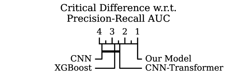
Figure 2. Critical Difference Plot (Brazdil and Soares, 2000) between models at $\alpha=0.1$. Numbers indicate each model’s average ranking on the single domain prediction tasks (Section 6.1), while the thick dark line connects models which are not significantly different from one another. This demonstrates that Our Model, which uses pretraining and models missing data, significantly outperforms CNNs, XGBoost, and CNN-Transformers across tasks (average rank=1.0).

6.2. Experiment 2: Comparison of Self-Supervised Pretraining Methods

Next we compare the three pretraining techniques proposed in Section 3.2 on the “Flu Symptoms” task (Section 6.1). This “Flu Symptoms” task has the least extreme class imbalance (1:37) and therefore yields highest statistical power to differentiate model performance. We use the following pretraining method:

1. Pretrain the model using all seven day windows in the train dataset.

2. Freeze the model’s CNN and transformer layers. If the pretraining technique used a classification head, randomize its parameters. If instead a regression head was used, replace it with a randomly initialized classification head.

3. Finetune the model on the target task (“Flu Symptoms”, in this case).

For all experiments, we use all of the model features described in Section (3.1) (i.e., the convolutional encoder, transformer blocks, and missingness flags). For comparison, we include a “No Pretraining” baseline, which shows the performance of a randomly initialized model.

Results. ROC and Precision Recall curves for this experiment are available in Figure 3. “Domain Inspired Features” pretraining, which trains the model to predict a pre-computed set of handcrafted features (Section 3.2), significantly outperforms other pretraining techniques and a randomly initialized model with a 16% improvement in PR AUC. Notably, the model pretrained on the “Same User” task does significantly worse than the others.

We additionally compared this pretraining-fine tuning approach to a multitask learning where both the pretraining and the target prediction objective are optimized concurrently. We repeated this comparison for each of the pretraining tasks (Section 3.2) in combination with the “Flu Symptoms” task. This strategy produced no meaningful improvement over the randomly initialized model, indicating that unsupervised pretraining is a superior paradigm for this setting. In addition, the pretraining-finetuning paradigm enables us to separate these two steps across two datasets, especially when the target dataset is relatively small. This is the focus of the next two experiments.

6.3. Experiment 3: Transfer learning improves flu prediction performance on small datasets in a repeated simulation study

Labeled behavioral data is often prohibitively expensive to collect, particularly in the context of public health where ground-truth labels require costly testing infrastructure and study management. Accordingly, many studies from prior work operate on data with on the order of dozen participants (Xu et al., 2021). In this regard, one promising application of generalizable self-supervised pretraining is that models could leverage large unlabeled datasets to improve predictive power in settings with limited labeled training data. Here, we repeatedly simulate such settings to robustly investigate whether such transfer learning leads to performance improvements.

First, we isolate all 4,989 study participants who never tested positive for the flu. We treat this set as a large, unlabeled dataset which we use to pretrain our model on the self-supervised “Daily Features” task (Section 3.2). We then take the remaining 206 users who did test positive at some point during the study, and randomly split this set into twenty folds of ten or eleven users each. This ensures that source and target domain share no participants in common. We provide an overview of this split in Figure A.2.

Next, for each fold we finetune the model on the supervised “Flu Positivity” task using data from the fold, and evaluate it on the users in the remaining nineteen folds. We choose this task as it mirrors the zero shot setting in the external dataset of Experiment 4. In both of these settings, all test subjects tested positive at some point and the predictive model attempts to predict on which day they do so. This process simulates finetuning the model with fewer than a dozen users’ data. We compare this approach to two non-pretrained models that only have access to the smaller target domain dataset: CNN-Transformer, and XGBoost trained on manually defined features (Table 2).

Results. We find that our pretrained model outperforms non-pretrained models on the “Flu Positivity” task when trained on fewer than a dozen participants (Figure 4). Pretraining alone increases average performance from 0.626 ROC AUC to 0.665, and 0.017 PR AUC to 0.021 (both $p<0.05$, Mann-Whitney U). This indicates that Our Model can learn generalizable features from unlabeled training data.

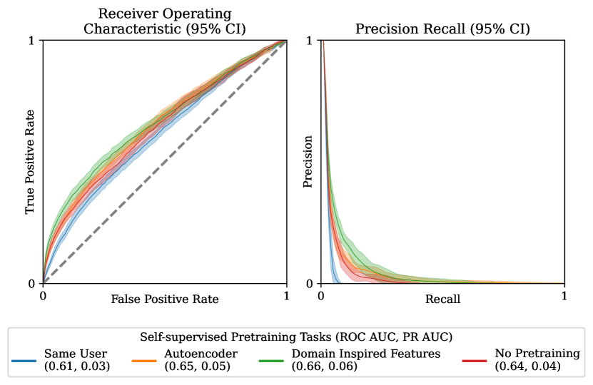
Figure 3. Comparison of self-supervised pretraining tasks (Section 3.2) on the “Flu Symptoms” task. The “Domain Inspired Features” task, which integrates domain knowledge, performs best relative to a non-pretrained model.

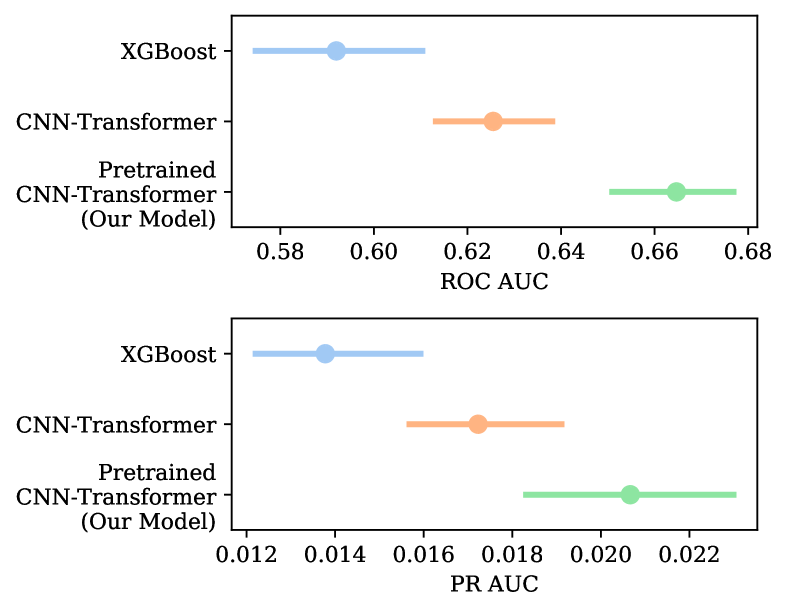
Figure 4. Comparison of XGBoost, CNN-Transformer, and a pretrained CNN-Transformer (Our Model) on the “Flu Positivity” task (Section 6.1) using training data from ten participants. Neural models outperform XGBoost, and pretraining yields additional improvement. This indicates that pretraining helps models generalize to tasks with limited training data. Horizontal lines represent 95% confidence intervals. Differences in means are significantly significant (all $p\leq 0.05$; Mann-Whitney U).

6.4. Experiment 4: Pretrained behavioral representations enable zero-shot COVID-19 prediction in small external dataset

	XGBoost	Our Model
Zero-shot PR AUC	0.005	0.018
Zero-shot ROC AUC	0.51	0.68

Table 3. Performance on zero-shot COVID-19 Prediction (Section 6.4). Our model’s superior performance indicates that CNN-Transformers pretrained on the “Domain Inspired Features” task (Section 3.2) learn generalizable features which transfer to new domains.

Finally, we use a small, independently collected dataset of FitBit recordings and COVID-19 test results to show that Our Model  can learn representations which generalize to entirely unseen diseases. This dataset contains 1470 total days of data for 32 individuals who tested positive with COVID-19 (Mishra et al., 2020). The original study authors use a very different prediction task (retrospective prediction with no train/test split), and so it is not possible to make a direct comparison between our model and theirs, but this dataset allows us to test our model’s performance on an unseen disease.

It is plausible that a self-supervised pretrained model, which in Experiment 1-3 showed good performance on flu related tasks, could support non-random predictive performance in a zero shot setting for COVID-19, as both are highly contagious respiratory viral infections which share symptoms and which may share a similar behavioral and physiological response to the disease (e.g., a change in resting heart rate around symptom onset (Shapiro et al., 2021)).

We pretrain our model with the “Domain Inspired Features” task (Section 3.2) and finetune it on the “Predict Flu Positivity” task (Section 3.2). Note that this is the same configuration as “Our Model” in Table 1. Then, with no additional supervision we use the model to predict COVID-19 positivity for each user on each day in the small, external dataset. As a zero-shot baseline using the data, we calculate a set of day-level features (Table A.2) from these data “and” our original flu dataset (Section 4) and train XGBoost using these features on the “Flu Prediction” task. Note that neither Our Model nor the XGBoost baseline is exposed to “any” data from the COVID-19 dataset during training.

Results. Our Model outperforms XGBoost on this zero-shot task, achieving 0.68 ROC AUC, while XGBoost predicts at 0.51 ROC AUC (about random chance) (Table 3). This illustrates the feasibility of pretrained CNN-Transformers for novel disease prediction, and shows that the features learned by our model are general enough to effectively transfer between these domains.

7. Discussion & Conclusion

In the COVID-19 pandemic rapid, cheap, over-the-counter antigen tests have been successfully deployed in surveillance testing, but the frequency of tests, more so than their sensitivity, remains a barrier to success in mitigating spread (Larremore et al., 2020). In this paper, we outlined a framework for evaluating mobile sensing methods for respiratory viral infection prediction on realistic tasks (Section 5) such as predicting flu positivity for every participant on every day of a flu season. While there are of course limitations to this work (e.g., a single flu season of data, limited sample size, restricted to flu and COVID-19 domains, limited interpretability of learned representations), we are able to report performance on par with COVID-19 rapid diagnostic tests, which have been found to have a ROC AUC of 0.84 (compared to 0.887 here on flu prediction; Table 1) in similar surveillance settings (Hirotsu et al., 2020). Certainly, more work is necessary to demonstrate similar performance levels in the same study population when deployed in a large-scale surveillance study. However, our findings demonstrate the potential of mobile sensing predictions as a complement to rapid antigen testing or as a trigger for additional testing. Specifically, our results indicate that pretraining, transformer self-attention, modeling missing data, and transfer learning are effective techniques in learning generalizable behavioral representations for mobile sensing.

Appendix A Reproducability Appendix

A.1. Hyperparameter Tuning

All models in this paper were trained with a randomized hyperparameter sweep using a withheld validation set. For CNN modules, we experimented with kernel sizes as large as 63, stride sizes as large as 256, depths as deep as eight layers, and as many as 32 output channels. For transformers modules, we experimented pre-computed and fixed positional embeddings, up to twelve layers of stacked transformers, and up to nine-head attention. We also tried dropout rates between 0.0 and 0.5. In total, over five hundred model configurations were tested before setting on the final configuration of kernel sizes of 5,5,2, stride sizes of 5,3,2, output channels of 8,16,32, two transformer layers each with four heads, and dropout of 0.4. We tried Adam learning rates from 1 to $1e-6$, and found that $5e-4$ worked best. This relatively small learning rate seemed to be important for limiting overfitting. We also conducted a hyperparameter sweep for XGBoost models, and found little low to hyperparameters, and that $\eta=1$ and a maximum depth of six worked best. Further, we experimented with window sizes ranging from three to ten days, and found that the model overfitted on both ends of this range, with best performance at seven days.

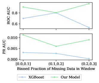
Figure A.1. Performance on the “Flu Positivity” task for binned levels of missing data. Missingness is defined as the fraction of minutes with heart rate data over the duration of the accompanying seven day window. 90% of labels have less that 30% missingness, making positive labels sparse, and so we do not compare methods past this threshold.

Feature	Description
Number of participants	5196
Average number of days of data	114
Portion of days containing missing data	93%
Mean age ($\pm$SD)	37.7 (10.2)
Portion Female	72%
Mean BMI ($\pm$SD)	30.3 (20.3)
Number of US States Represented	50

Table A.1. Summary statistics for the Homekit Flu Monitoring Study (Section 4)

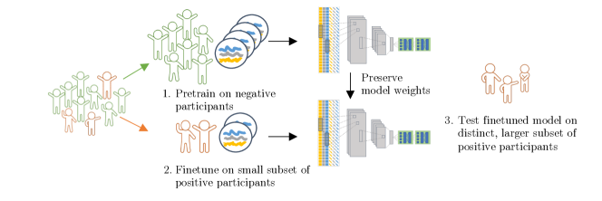
Figure A.2. Overview of the cross validation split for our simulation of small datasets (Section 6.3)

Feature	Description
Resting HR 95th Pct	95th percentile of resting HR
Resting HR 50th Pct	50th percentile of resting HR
Resting HR std.	Standard deviation of resting HR
Awake HR 95th Pct	95th percentile of HR while awake
Steps Streak 95th Pct	95th percentile of continuous steps
Steps Streak 50th Pct	50th percentile of continuous steps
Total Minutes in Bed	Number of minutes spent in bed during duration
Sleep Minutes	Number of minutes spent asleep during duration
Total Steps	Total Number of steps during duration
Missing HR	Indicator for missing HR data
Missing Sleep	Indicator for missing sleep data
Missing Steps	Indicator for missing steps
Missing Day	Indicator for missing all data

Table A.2. Summary of manually defined features used for XGBoost baseline in the zero shot experiment (Section 6.4) calculated for every user and on each day. “Missing” features are binary variables which are 1 if more than one hour of data is missing, and 0 otherwise.

References

- (1)
- cdc (2021a) 2021a. Estimated Flu-Related Illnesses, Medical visits, Hospitalizations, and Deaths in the United States — 2018–2019 Flu Season | CDC.
- cdc (2021b) 2021b. Influenza Signs and Symptoms and the Role of Laboratory Diagnostics.
- Bachman et al. (2021) Christine M. Bachman, Benjamin D. Grant, Caitlin E. Anderson, Luis F. Alonzo, Spencer Garing, et al. 2021. Clinical validation of an open-access SARS-COV-2 antigen detection lateral flow assay, compared to commercially available assays. PLOS ONE (2021).
- Beltagy et al. (2020) Iz Beltagy, Matthew E. Peters, and Arman Cohan. 2020. Longformer: The Long-Document Transformer. arXiv:2004.05150 [cs] (2020).
- Brazdil and Soares (2000) Pavel B. Brazdil and Carlos Soares. 2000. A Comparison of Ranking Methods for Classification Algorithm Selection. In Machine Learning: ECML 2000, Jaime G. Carbonell, Jörg Siekmann, G. Goos, J. Hartmanis, J. van Leeuwen, et al. (Eds.). Springer Berlin Heidelberg, Berlin, Heidelberg.
- Brook et al. (2021) Cara E. Brook, Graham R. Northrup, Alexander J. Ehrenberg, Jennifer A. Doudna, and Mike Boots. 2021. Optimizing COVID-19 control with asymptomatic surveillance testing in a university environment. Epidemics (2021).
- Buda et al. (2021) Teodora Sandra Buda, Mohammed Khwaja, and Aleksandar Matic. 2021. Outliers in Smartphone Sensor Data Reveal Outliers in Daily Happiness. Proceedings of the ACM on Interactive, Mobile, Wearable and Ubiquitous Technologies (2021).
- Cao et al. (2017) Bokai Cao, Lei Zheng, Chenwei Zhang, Philip S Yu, Andrea Piscitello, et al. 2017. Deepmood: modeling mobile phone typing dynamics for mood detection. In KDD.
- Chen et al. (2020) Hugh Chen, Scott Lundberg, Gabe Erion, Jerry H Kim, and Su-In Lee. 2020. Forecasting adverse surgical events using self-supervised transfer learning for physiological signals. arXiv:2002.04770 (2020).
- Chu et al. (2012) Haitao Chu, Eric T. Lofgren, M. Elizabeth Halloran, Pei F. Kuan, Michael Hudgens, et al. 2012. Performance of rapid influenza H1N1 diagnostic tests: a meta-analysis. Influenza and Other Respiratory Viruses (2012).
- Chu et al. (2020) Helen Y. Chu, Janet A. Englund, Lea M. Starita, Michael Famulare, Elisabeth Brandstetter, et al. 2020. Early Detection of Covid-19 through a Citywide Pandemic Surveillance Platform. New England Journal of Medicine (2020).
- DeLong et al. (1988) Elizabeth R. DeLong, David M. DeLong, and Daniel L. Clarke-Pearson. 1988. Comparing the Areas under Two or More Correlated Receiver Operating Characteristic Curves: A Nonparametric Approach. Biometrics (1988).
- Devlin et al. (2019) Jacob Devlin, Ming-Wei Chang, Kenton Lee, and Kristina Toutanova. 2019. BERT: Pre-training of Deep Bidirectional Transformers for Language Understanding. In NAACL-HLT (1).
- Fawaz et al. (2019) Hassan Ismail Fawaz, Germain Forestier, Jonathan Weber, Lhassane Idoumghar, and Pierre-Alain Muller. 2019. Deep learning for time series classification: a review. 33, 4 (July 2019), 917–963. arXiv: 1809.04356.
- Friedman (1940) Milton Friedman. 1940. A Comparison of Alternative Tests of Significance for the Problem of $m$ Rankings. (1940), 86–92.
- Fusco et al. (2020) F. M. Fusco, M. Pisaturo, V. Iodice, R. Bellopede, O. Tambaro, et al. 2020. COVID-19 among healthcare workers in a specialist infectious diseases setting in Naples, Southern Italy: results of a cross-sectional surveillance study. Journal of Hospital Infection (2020).
- Hafiz et al. (2020) Pegah Hafiz, Kamilla Woznica Miskowiak, Alban Maxhuni, Lars Vedel Kessing, and Jakob Eyvind Bardram. 2020. Wearable Computing Technology for Assessment of Cognitive Functioning of Bipolar Patients and Healthy Controls. IMWUT (2020).
- Haibo He and Garcia (2009) Haibo He and E.A. Garcia. 2009. Learning from Imbalanced Data. IEEE Transactions on Knowledge and Data Engineering (2009), 1263–1284.
- Hallgrímsson et al. (2018) Haraldur T Hallgrímsson, Filip Jankovic, Tim Althoff, and Luca Foschini. 2018. Learning individualized cardiovascular responses from large-scale wearable sensors data. NeurIPS ML4H (2018).
- He et al. (2016) Kaiming He, Xiangyu Zhang, Shaoqing Ren, and Jian Sun. 2016. Deep residual learning for image recognition. In Proceedings of the IEEE conference on computer vision and pattern recognition. 770–778.
- Hirotsu et al. (2020) Yosuke Hirotsu, Makoto Maejima, Masahiro Shibusawa, Yuki Nagakubo, Kazuhiro Hosaka, et al. 2020. Comparison of automated SARS-CoV-2 antigen test for COVID-19 infection with quantitative RT-PCR using 313 nasopharyngeal swabs, including from seven serially followed patients. International Journal of Infectious Diseases 99 (Oct. 2020), 397–402.
- Hochreiter and Schmidhuber (1997) Sepp Hochreiter and Jürgen Schmidhuber. 1997. Long short-term memory. Neural computation (1997), 1735–1780.
- International Monetary Fund (2020) International Monetary Fund. 2020. A Crisis Like No Other, An Uncertain Recovery.
- Ismail et al. (2020) Mahmoud Al Ismail, Soham Deshmukh, and Rita Singh. 2020. Detection of COVID-19 through the analysis of vocal fold oscillations. (2020).
- Jaques et al. (2017) Natasha Jaques, Ognjen (Oggi) Rudovic, Sara Taylor, Akane Sano, and Rosalind Picard. 2017. Predicting Tomorrow’s Mood, Health, and Stress Level using Personalized Multitask Learning and Domain Adaptation. In Proceedings of IJCAI 2017 Workshop on Artificial Intelligence in Affective Computing.
- Kingma and Ba (2017) Diederik P. Kingma and Jimmy Ba. 2017. Adam: A Method for Stochastic Optimization.
- Kiranyaz et al. (2021) Serkan Kiranyaz, Onur Avci, Osama Abdeljaber, Turker Ince, Moncef Gabbouj, et al. 2021. 1D convolutional neural networks and applications: A survey. Mechanical Systems and Signal Processing (2021).
- Kolbeinsson et al. (2021) Arinbjörn Kolbeinsson, Piyusha Gade, Raghu Kainkaryam, Filip Jankovic, and Luca Foschini. 2021. Self-supervision of wearable sensors time-series data for influenza detection. arXiv:2112.13755 [cs] (Dec. 2021).
- Krizhevsky et al. (2012) Alex Krizhevsky, Ilya Sutskever, and Geoffrey E Hinton. 2012. Imagenet classification with deep convolutional neural networks. NeurIPS (2012).
- Lan et al. (2019) Zhenzhong Lan, Mingda Chen, Sebastian Goodman, Kevin Gimpel, Piyush Sharma, et al. 2019. Albert: A lite bert for self-supervised learning of language representations. arXiv preprint arXiv:1909.11942 (2019).
- Laport-López et al. (2020) Francisco Laport-López, Emilio Serrano, Javier Bajo, and Andrew T. Campbell. 2020. A review of mobile sensing systems, applications, and opportunities. Knowledge and Information Systems (2020).
- Larremore et al. (2020) Daniel B. Larremore, Bryan Wilder, Evan Lester, Soraya Shehata, James M. Burke, et al. 2020. Test sensitivity is secondary to frequency and turnaround time for COVID-19 surveillance. medRxiv (Sept. 2020).
- Lewis et al. (2019) Mike Lewis, Yinhan Liu, Naman Goyal, Marjan Ghazvininejad, Abdelrahman Mohamed, et al. 2019. Bart: Denoising sequence-to-sequence pre-training for natural language generation, translation, and comprehension. (2019).
- Li and Sano (2020) Boning Li and Akane Sano. 2020. Extraction and Interpretation of Deep Autoencoder-based Temporal Features from Wearables for Forecasting Personalized Mood, Health, and Stress. IMWUT (2020).
- Lin et al. (2020) Zongyu Lin, Shiqing Lyu, Hancheng Cao, Fengli Xu, Yuqiong Wei, et al. 2020. HealthWalks: Sensing Fine-grained Individual Health Condition via Mobility Data. IMWUT (2020), 1–26.
- Liu et al. (2022) Shuo Liu, Jing Han, Estela Laporta Puyal, Spyridon Kontaxis, Shaoxiong Sun, et al. 2022. Fitbeat: COVID-19 estimation based on wristband heart rate using a contrastive convolutional auto-encoder. Pattern Recognition (2022).
- Liu et al. (2019) Yinhan Liu, Myle Ott, Naman Goyal, Jingfei Du, Mandar Joshi, et al. 2019. Roberta: A robustly optimized bert pretraining approach. arXiv:1907.11692 (2019).
- Logeswaran and Lee (2018) Lajanugen Logeswaran and Honglak Lee. 2018. An efficient framework for learning sentence representations.
- Ma et al. (2020) Yuchao Ma, Andrew T Campbell, Diane J Cook, John Lach, Shwetak N Patel, et al. 2020. Transfer learning for activity recognition in mobile health. (2020).
- Mairittha et al. (2021) Nattaya Mairittha, Tittaya Mairittha, Paula Lago, and Sozo Inoue. 2021. CrowdAct: Achieving High-Quality Crowdsourced Datasets in Mobile Activity Recognition. IMWUT (2021).
- Malik et al. (2020) Momin M. Malik, Afsaneh Doryab, Michael Merrill, Jürgen Pfeffer, and Anind K. Dey. 2020. Can Smartphone Co-locations Detect Friendship? It Depends How You Model It. arXiv:2008.02919 [cs] (2020).
- McDermott et al. (2021) Matthew BA McDermott, Shirly Wang, Nikki Marinsek, Rajesh Ranganath, Luca Foschini, et al. 2021. Reproducibility in machine learning for health research: Still a ways to go. Science Translational Medicine (2021).
- Meegahapola et al. (2021) Lakmal Meegahapola, Salvador Ruiz-Correa, Viridiana del Carmen Robledo-Valero, Emilio Ernesto Hernandez-Huerfano, Leonardo Alvarez-Rivera, et al. 2021. One More Bite? Inferring Food Consumption Level of College Students Using Smartphone Sensing and Self-Reports. IMWUT (2021).
- Mercer and Salit (2021) Tim R. Mercer and Marc Salit. 2021. Testing at scale during the COVID-19 pandemic. Nature Reviews Genetics (2021).
- Mezlini et al. (2021) Aziz Mezlini, Allison Shapiro, Eric J Daza, Eamon Caddigan, Ernesto Ramirez, et al. 2021. Estimating the Burden of Influenza on Daily Activity at Population Scale Using Commercial Wearable Sensors. medRxiv (2021).
- Mikolov et al. (2013) Tomas Mikolov, Ilya Sutskever, Kai Chen, Greg S Corrado, and Jeff Dean. 2013. Distributed representations of words and phrases and their compositionality. In Advances in neural information processing systems. 3111–3119.
- Mishra et al. (2020) Tejaswini Mishra, Meng Wang, Ahmed A. Metwally, Gireesh K. Bogu, Andrew W. Brooks, et al. 2020. Pre-symptomatic detection of COVID-19 from smartwatch data. Nature Biomedical Engineering (2020).
- Nair et al. (2019) Suraj Nair, Kiran Javkar, Jiahui Wu, and Vanessa Frias-Martinez. 2019. Understanding Cycling Trip Purpose and Route Choice Using GPS Traces and Open Data. IMWUT (2019).
- Natarajan et al. (2020) Aravind Natarajan, Hao-Wei Su, and Conor Heneghan. 2020. Assessment of physiological signs associated with COVID-19 measured using wearable devices. Nature Digital Medicine (2020).
- Nestor et al. (2021) Bret Nestor, Jaryd Hunter, Raghu Kainkaryam, Erik Drysdale, Jeffrey B Inglis, et al. 2021. Dear Watch, Should I Get a COVID-19 Test? Designing deployable machine learning for wearables. medRxiv (2021).
- Ni et al. (2019) Jianmo Ni, Larry Muhlstein, and Julian McAuley. 2019. Modeling heart rate and activity data for personalized fitness recommendation. In WWW.
- Pyrkov et al. (2018) Timothy V. Pyrkov, Konstantin Slipensky, Mikhail Barg, Alexey Kondrashin, Boris Zhurov, et al. 2018. Extracting biological age from biomedical data via deep learning: too much of a good thing? Scientific Reports (2018).
- Quer et al. (2020) Giorgio Quer, Jennifer M. Radin, Matteo Gadaleta, Katie Baca-Motes, Lauren Ariniello, et al. 2020. Wearable sensor data and self-reported symptoms for COVID-19 detection. Nature Medicine (2020).
- Saito and Rehmsmeier (2015) Takaya Saito and Marc Rehmsmeier. 2015. The Precision-Recall Plot Is More Informative than the ROC Plot When Evaluating Binary Classifiers on Imbalanced Datasets. PLoS ONE (2015).
- Shapiro et al. (2021) Allison Shapiro, Nicole Marinsek, Ieuan Clay, Benjamin Bradshaw, Ernesto Ramirez, et al. 2021. Characterizing COVID-19 and influenza illnesses in the real world via person-generated health data. Patterns (2021), 100188.
- Shen et al. (2019) Yichen Shen, Maxime Voisin, Alireza Aliamiri, Anand Avati, Awni Hannun, et al. 2019. Ambulatory Atrial Fibrillation Monitoring Using Wearable Photoplethysmography with Deep Learning. In KDD.
- Song et al. (2018) Huan Song, Deepta Rajan, Jayaraman J Thiagarajan, and Andreas Spanias. 2018. Attend and diagnose: Clinical time series analysis using attention models. In AAAI.
- Spathis et al. (2019) Dimitris Spathis, Sandra Servia-Rodriguez, Katayoun Farrahi, Cecilia Mascolo, and Jason Rentfrow. 2019. Sequence multi-task learning to forecast mental wellbeing from sparse self-reported data. In KDD.
- Suhara et al. (2017) Yoshihiko Suhara, Yinzhan Xu, and Alex’Sandy’ Pentland. 2017. Deepmood: Forecasting depressed mood based on self-reported histories via recurrent neural networks. In WWW.
- Tang et al. (2021) Chi Ian Tang, Ignacio Perez-Pozuelo, Dimitris Spathis, Soren Brage, Nick Wareham, et al. 2021. SelfHAR: Improving Human Activity Recognition through Self-training with Unlabeled Data. arXiv:2102.06073 (2021).
- Vaswani et al. (2017) Ashish Vaswani, Noam Shazeer, Niki Parmar, Jakob Uszkoreit, Llion Jones, et al. 2017. Attention is all you need. In Advances in neural information processing systems. 5998–6008.
- Wang et al. (2019) Jindong Wang, Yiqiang Chen, Shuji Hao, Xiaohui Peng, and Lisha Hu. 2019. Deep learning for sensor-based activity recognition: A survey. Pattern Recognition Letters (2019).
- Wang et al. (2016) Rui Wang, Min SH Aung, Saeed Abdullah, Rachel Brian, Andrew T Campbell, et al. 2016. CrossCheck: toward passive sensing and detection of mental health changes in people with schizophrenia. In UbiComp.
- Wang et al. (2014) Rui Wang, Fanglin Chen, Zhenyu Chen, Tianxing Li, Gabriella Harari, et al. 2014. StudentLife: assessing mental health, academic performance and behavioral trends of college students using smartphones. In UbiComp.
- Wu et al. (2020) Xian Wu, Chao Huang, Pablo Roblesgranda, and Nitesh Chawla. 2020. Representation learning on variable length and incomplete wearable-sensory time series. (2020).
- Xu et al. (2021) Xuhai Xu, Jennifer Mankoff, and Anind K. Dey. 2021. Understanding Practices and Needs of Researchers in Human State Modeling by Passive Mobile Sensing.
- Yao et al. (2017) Shuochao Yao, Shaohan Hu, Yiran Zhao, Aston Zhang, and Tarek Abdelzaher. 2017. Deepsense: A unified deep learning framework for time-series mobile sensing data processing. In WWW.
- Zerveas et al. (2021) George Zerveas, Srideepika Jayaraman, Dhaval Patel, Anuradha Bhamidipaty, and Carsten Eickhoff. 2021. A Transformer-based Framework for Multivariate Time Series Representation Learning. In KDD.
- Zhang et al. (2019) Chuxu Zhang, Dongjin Song, Yuncong Chen, Xinyang Feng, Cristian Lumezanu, et al. 2019. A Deep Neural Network for Unsupervised Anomaly Detection and Diagnosis in Multivariate Time Series Data. AAAI (July 2019).
- Zhang et al. (2021) Yunke Zhang, Fengli Xu, Tong Li, Vassilis Kostakos, Pan Hui, et al. 2021. Passive Health Monitoring Using Large Scale Mobility Data. IMWUT (2021).