AGP-based unitary coupled cluster theory for quantum computers

Abstract

Electronic structure methods typically benefit from symmetry breaking and restoration, specially in the strong correlation regime. The same goes for Ansätze on a quantum computer. We develop a unitary coupled cluster method based on the antisymmetrized geminal power (AGP)—a state formally equivalent to the number-projected Bardeen–Cooper–Schrieffer wavefunction. We demonstrate our method for the single-band Fermi–Hubbard Hamiltonian in one and two dimensions. We also explore post-selection as a state preparation step to obtain correlated AGP and prove that it scales no worse than $\mathcal{O}(\sqrt{M})$ in the number of measurements, thereby making it a less expensive alternative to gauge integration to restore particle number symmetry.

I Introduction

One of the most sought after applications of quantum computers is to solve the strong correlation problem in electronic structure theory Cao et al. (2019); McArdle et al. (2020). Electronic structure methods often start from a mean-field state, typically a Hartree–Fock (HF) Slater determinant, and are systematically improved using a variety of techniques Helgaker et al. (2000). When electronic correlation is weak, single reference coupled cluster theory (CC) is known to be sufficiently accurate in quantum chemistry and is often regarded as the gold-standard Scuseria et al. (1987); Bartlett and Musiał (2007). However, in the strongly correlated regime, many Slater determinants become equally dominant and single-reference methods often struggle Bulik et al. (2015).

Strong correlation in finite systems typically manifest itself by breaking one or more symmetries at the mean-field level. In this case, one could either make the mean-field state retain desired symmetries and correlate it in a symmetry-adapted manner, or, one could allow the symmetries to break and correlate the symmetry-broken mean-field state Ring and Schuck (1980); Blaizot and Ripka (1986). The trade-off between these two strategies is that the broken symmetry wavefunction gives a lower energy at the expense of a less accurate wavefunction due to the lack of correct symmetries. This is known as the symmetry dilemma in electronic structure theory Löwdin (1955); Lykos and Pratt (1963); Scuseria et al. (2011); Jiménez-Hoyos et al. (2012) and extends to traditional and unitary coupled cluster theory alike Evangelista (2011); Duguet (2015); Qiu et al. (2017).

In recent years, there has been extensive interest in using physically inspired Ansätze in variational quantum algorithms Cerezo et al. (2021). In electronic structure calculations, the disentangled form of unitary CC (uCC) is perhaps the most natural extension of physically inspired Ansätze that can be implemented on a quantum computer Shen et al. (2017); Tilly et al. (2021); Anand et al. (2022). For example, one can write down the uCC Ansatz as

$$|{\psi(\vec{t})}\rangle=\prod_{k}e^{t_{k}\left(\hat{{\tau}}_{k}-\hat{{\tau}}^{\dagger}_{k}\right)}|{\phi}\rangle,$$ (1)

where $|{\phi}\rangle$ is a mean-filed reference, $\hat{{\tau}}_{k}$ is the $k{\text{-th}}$ excitation operator which can be symmetry-adapted or broken, and $t_{k}$ is the corresponding amplitude Evangelista et al. (2019); Grimsley et al. (2020); Izmaylov et al. (2020a). We can variationally minimize the energy,

$$E(\vec{t})=\langle{\psi(\vec{t})}|H|{\psi(\vec{t})}\rangle,$$ (2)

using the variationally quantum eigensolver (VQE) in a hybrid quantum–classical optimization manner Peruzzo et al. (2014); McClean et al. (2016). To address the ambiguity in the ordering of the operators and the depth of the uCC Ansatz, heuristics such as the ADAPT-VQE Grimsley et al. (2019) have been developed and extended over the years Tang et al. (2021); Grimsley et al. (2022); Romero et al. (2022). Other notable works along this direction are the qubit coupled cluster approach Ryabinkin et al. (2018, 2020), cluster-Jastrow Ansatz Matsuzawa and Kurashige (2020), k-UpCCGSD Lee et al. (2019), and the projective quantum eigensolver (PQE) Stair and Evangelista (2021) among others Kandala et al. (2017); Dallaire-Demers et al. (2019); Izmaylov et al. (2020a); Xia and Kais (2020); Anselmetti et al. (2021). Combining VQE Ansätze with quantum Monte Carlo has been recently proposed as well Huggins et al. (2022).

An important consideration among all methods for noisy intermediate–scale quantum (NISQ) devices is how deep an Ansatz needs to be in order to achieve sufficient accuracy Preskill (2018); Leymann and Barzen (2020) in the strongly correlated regime. For example, when using a symmetry-adapted Ansatz, it is conceivable that more collective excitations are needed to recover the same level of accuracy in energy as those of symmetry-broken Ansätze in the regimes where symmetries break. This could require a larger number of variational parameters and deeper circuits to implement, which, in some cases, could scale exponentially.

A remedy for this problem could be to combine symmetry restoration with CC theory Duguet (2015); Qiu et al. (2017); Duguet and Signoracci (2017); Wahlen-Strothman et al. (2017); Qiu et al. (2019); Song et al. (2022). Symmetry breaking and restoration has long been studied in nuclear physics and electronic structure theory Ring and Schuck (1980); Scuseria et al. (2011); Jiménez-Hoyos et al. (2012); Sheikh et al. (2021). It has also gained attention for applications on quantum computers in recent years. Restoration of parity, $S^{2}$, $S_{z}$, translational, and other symmetries on a quantum computer have been proposed Izmaylov (2019); Yen et al. (2019); Tsuchimochi et al. (2020); Seki et al. (2020); Lacroix (2020); Siwach and Lacroix (2021); Seki and Yunoki (2022); Ruiz Guzman and Lacroix (2022). Some of the authors of this paper have shown how to efficiently restore particle number symmetry over the BCS wavefunction on a quantum computer Khamoshi et al. (2020). The projected BCS wavefunction is known as the antisymmetrized geminal power (AGP) whose claim to fame is its ability to capture off-diagonal long-range order (ODLRO) without breaking number symmetry Yang (1962); Coleman (1965); Sager and Mazziotti (2022). Common electronic structure methods, including HF and density functional theory, fail to capture ODLRO. Combining uCC with AGP is the central goal of this paper.

Number symmetry often breaks spontaneously for systems where the effective two-body interaction is attractive. The prime example is superconductivity or the superfluid phase in condensed matter and nuclear physics Bardeen et al. (1957); Brink and Broglia (2005); Sedrakian and Clark (2019). Number symmetry does not typically break in molecules Bach et al. (1994). However the AGP wavefunction has a long history in quantum chemistry as well, and it is connected to the concept of bonding Surján (1999). AGP, by itself, is usually insufficient to accurately describe molecular systems, but it could be a good starting point for correlated methods such as configuration interactions or coupled cluster theory Henderson and Scuseria (2019); Khamoshi et al. (2019); Dutta et al. (2020); Henderson and Scuseria (2020); Dutta et al. (2021); Khamoshi et al. (2021). AGP-based quantum Monte Carlo methods have been used extensively over the years for molecules and solids Casula and Sorella (2003); Casula et al. (2004); Wei and Neuscamman (2018); Genovese et al. (2019); Genovese and Sorella (2020). Neuscamman has shown that variational Jastrow correlators on AGP is fully size-consistent and highly accurate Neuscamman (2013a, b). Ref. Matsuzawa and Kurashige (2020) developed a unitary analogue of this theory, although the authors were not aware of an efficient implementation of AGP on a quantum computer. Other geminal-based methods include using Richardson-Gaudin wavefunction Fecteau et al. (2020a); Johnson et al. (2020, 2021); Fecteau et al. (2020b, 2022); Moisset et al. (2022), which although are not done on a quantum computer, they are relevant to AGP.

In Ref. Khamoshi et al. (2020) we demonstrated an efficient correlated AGP method on a quantum computer in the seniority-zero space. Our goal in this paper is to show how our previous formalism can be extended beyond seniority-zero systems and onto general ab initio Hamiltonians. To this end, we develop a unitary coupled cluster Ansatz atop of AGP and benchmark our numerical method against the ground state of the single-band Fermi–Hubbard model. The Hubbard Hamiltonian breaks number symmetry when the on-site interaction is attractive; and, when the on-site interactions is repulsive, it features strong correlation prototypical of those that occur in molecules. Our intent is to demonstrate our method in both regimes of this Hamiltonian.

Another contribution of this paper is to exploit post-measurement selection, or post-selection in short, as an alternative to the $U(1)$ gauge integral in restoring number symmetry. Post-selection has been widely used as a crucial error mitigation technique for calculations performed on NISQ hardware Endo et al. (2018); Bonet-Monroig et al. (2018); Kandala et al. (2019); Endo et al. (2021); Huggins et al. (2021). We show, however, how post-selection can be used in conjunction with uCC to sample over correlated AGP. Our primary contribution is to show that restoring number symmetry with post-selection could scale more favorably than gauge integration as judged by the circuit depth and number of measurements. We analytically prove an asymptotic bound of $\mathcal{O}(\sqrt{M})$ measurements and confirm it with computations based on a noise-free quantum emulator.

Restoring symmetries via post-selection is a distinct possibility that is not viable on classical computers but can be conveniently performed on a quantum computer. Indeed, post-selection can be combined with the integral or phase estimation Lacroix (2020) to restore multiple symmetries. Our general philosophy for methods in strong correlation is to allow multiple symmetries to break and later restore them in the presence of the correlator. This could pave the way for methods that work equally well in repulsive, attractive, weak, and strong correlation regimes.

This paper is organized as follows: We begin Sec. II by first reviewing some previous work and basic concepts, then we build our way to seniority nonzero methods in Sec. II.1. In Sec. II.2, we discuss the optimization of AGP state on classical and quantum computers and review a formal connection with number projected HFB. Sec. II.3 is devoted to disentangled uCC on AGP. Sec. III discusses post-selection; the procedure is discussed in Sec. III.1 and the numerical benchmarks are presented in Sec. III.2. In Sec. IV and the subsections therein, we demonstrate different uCC correlators based-on AGP and discuss our results for the Hubbard Hamiltonian. We conclude the paper with some final remarks in Sec. V.

II Theory

Define ${{{\Gamma}}}^{\dagger}$ to be the geminal creation operator,

$${{{\Gamma}}}^{\dagger}=\frac{1}{2}\sum_{pq}\eta_{pq}{c}^{\dagger}_{p}{c}^{\dagger}_{q},$$ (3)

where ${c}^{\dagger}_{p}$ is a fermionic creation operator in a spin-orbital $p$ and $\eta$ is an anti-symmetric matrix whose elements are known as the geminal coefficients. An AGP with $N$ pairs, or $2N$ electrons, can then be defined as Coleman (1965); Surján (1999)

$$|\text{AGP}\rangle=\frac{1}{N!}\left({{{\Gamma}}}^{\dagger}\right)^{N}|\text{vac}\rangle.$$ (4)

Unless otherwise specified, we choose to work in the natural orbital basis of the geminal wherein the matrix $\eta$ is brought to a quasi-diagonal form Hua (1944),

$$\bar{\eta}=\bigoplus_{p=1}^{M}\begin{pmatrix}0&\eta_{p}\\ -\eta_{p}&0\\ \end{pmatrix}=D^{\dagger}\eta D^{*},$$ (5)

via the orbital rotation

$${a}^{\dagger}_{p}=\sum_{q=1}^{2M}D_{qp}{c}^{\dagger}_{q},$$ (6)

where $D$ is the unitary matrix of natural orbital coefficients and $M$ is the number of spatial orbitals. As such, the geminal operator can be written as

$${{{\Gamma}}}^{\dagger}=\sum_{p=1}^{M}\eta_{p}{a}^{\dagger}_{p}{a}^{\dagger}_{\bar{p}},$$ (7)

where the natural orbitals $p$ and $\bar{p}$ are “paired” in the sense of Eq. (5). As shown in Appendix A, a $(p,\,\bar{p})$ pair reduces to a spin $(\uparrow,\,\downarrow)$ pair if the spins of the natural orbitals are collinear. With this pairing scheme, the relationship between AGP and the BCS wavefunction can be easily seen from

$$|\text{BCS}\rangle =\prod_{p=1}^{M}(u_{p}+v_{p}{a}^{\dagger}_{p}{a}^{\dagger}_{\bar{p}})|\text{vac}\rangle$$ (8a)

$$\propto\prod_{p=1}^{M}(1+\eta_{p}{a}^{\dagger}_{p}{a}^{\dagger}_{\bar{p}})|\text{vac}\rangle$$ (8b)

$$=\sum_{N=0}^{M}\frac{1}{N!}\left({{{\Gamma}}}^{\dagger}\right)^{N}|\text{vac}\rangle,$$ (8c)

where the BCS coefficients $\{u_{p},v_{p}\}$ relate to $\{\eta_{p}\}$ through $\eta_{p}=v_{p}/u_{p}$. Clearly the BCS wavefunction is a linear combination of AGPs with all possible number of electron pairs (up to an inconsequential normalization factor). The AGP of $N$ pairs, Eq. (4), corresponds to the projected BCS (PBCS) state with the correct particle number. The AGP ground state can be optimized on a classical computer at mean-field cost (see Sec. II.2).

II.1 Beyond zero seniority

Seniority is defined as the number of unpaired electrons and is denoted by $\Omega$ Ring and Schuck (1980). Any two-body ab initio Hamiltonian can be written as Henderson et al. (2015)

$$H=H^{\delta{\Omega}=0}+H^{\delta{\Omega}=\pm 2}+H^{\delta{\Omega}=\pm 4},$$ (9)

where the superscript differentiates between sectors of the Hamiltonian that change seniority by $0,\pm 2$ and $\pm 4$. The seniority-zero subspace features a remarkable simplicity Bytautas et al. (2011); Stein et al. (2014); Henderson et al. (2014); Bytautas et al. (2015); Shepherd et al. (2016), which makes it particularly convenient for quantum algorithms Khamoshi et al. (2020); Elfving et al. (2021). One can define a $su(2)$ pairing algebra with the generators

$$\mathbf{P}^{\dagger}_{p} ={a}^{\dagger}_{p}{a}^{\dagger}_{\bar{p}},$$ (10a)

$$\mathbf{N}_{p} ={a}^{\dagger}_{p}{a}_{p}+{a}^{\dagger}_{\bar{p}}{a}_{\bar{p}},$$ (10b)

and posit a paired encoding, $\mathbf{P}^{\dagger}_{p}\mapsto\frac{1}{2}({X}_{p}-i{Y}_{p})$ and $\mathbf{N}_{p}\mapsto 1-{Z}_{p}$, such that the qubit states $|{1}\rangle=\left(\begin{smallmatrix}0\\ 1\end{smallmatrix}\right)$ and $|{0}\rangle=\left(\begin{smallmatrix}1\\ 0\end{smallmatrix}\right)$ correspond to an electron-pair being present and absent respectively; here, $X,Y$, and $Z$ are Pauli matrices. Any seniority-zero Hamiltonian can be encoded as

$$H^{\delta\Omega=0} \mapsto\sum_{p}h_{p}{Z}_{p}+\sum_{pq}w_{pq}{Z}_{p}{Z}_{q}$$

$$\quad+\sum_{pq}v_{pq}\left({X}_{p}{X}_{q}+{Y}_{p}{Y}_{q}\right),$$ (11)

where $w$ and $v$ are Hermitian matrices. For most Hamiltonians, seniority is not a good quantum number, and the restriction to the seniority-zero subspace leads to approximate energies. Indeed, for ab initio Hamiltonians, doubly-occupied configuration interaction Veillard and Clementi (1967); Couty and Hall (1997); Kollmar and Heß (2003) (an exact diagonalization method in the seniority-zero subspace) is not sufficient to reach chemical accuracy. Therefore it becomes necessary to incorporate broken pair excitations.

@C=2em @R=1.5em —0⟩_a &H 1
—0⟩_1 R_y(θ_1) 1 3R_i
—0⟩_¯1 R_i
—0⟩_2 R_y(θ_2) 1 R_i
—0⟩_¯2 R_i 2233.9em– 4253.9em–

(a)

@C=1em @R=1.5em anc. & 1 1
1 3R_i R_z(ϕ_i)
¯1 R_i ⟹ 1
2 R_i R_z(ϕ_i)
¯2 R_i

(b)

Figure 1: Circuits to implement the number projected BCS wavefunction for seniority nonzero applications using the integral. Here it is shown for a system with 4 spin-orbitals ($M=2$) for simplicity. (a) Implementation of the BCS wavefunction and circuit to the do Hadamard test for every grid angle $\phi_{i}$. The dashed box implements $\exp{\left(i\theta_{p}\left({X}_{\bar{p}}{X}_{p}+{Y}_{\bar{p}}{Y}_{p}\right)/2\right)}$ acting on the vacuum state after simplification. (b) Implementation of the controlled $R_{z}(\phi_{i})$ using nearest neighbors connectivity. Since the BCS orbitals $p$ and $\bar{p}$ are either simultaneously present or absent, the controlled $R_{z}(\phi_{i})$ can be chosen to apply only to the “no-bar” qubits. The swap gates move the logical qubit of the ancilla qubit to the last qubit to measure $\langle{X_{a}}\rangle+i\langle{Y_{a}}\rangle$ needed for the Hadamard test.

To allow pairs to break, we first need to map individual spin-orbitals to qubits. Our goal is to follow our formalism for seniority-zero Khamoshi et al. (2020) closely to take advantage of its low asymptotic scaling and other desirable properties. We want to implement AGP, again, in its natural orbital basis where all electrons are paired. Broken-pair excitations then come from the correlator that couples the reference to all seniority sectors of the Hamiltonian.

We interlace the qubits associated with natural orbitals $p$ and $\bar{p}$ (i.e. logical qubits of $p$ ($\bar{p}$) correspond to odd (even) physical qubits), and adopt the Jordan–Wigner (JW) encoding of fermions Jordan and Wigner (1928), so that $a_{p}\mapsto\frac{1}{2}\left({X}_{p}+i{Y}_{p}\right){Z}_{\bar{p}-1}{Z}_{p-1}\cdots{Z}_{\bar{1}}{Z}_{1}$ and $a_{\bar{p}}\mapsto\frac{1}{2}\left({X}_{\bar{p}}+i{Y}_{\bar{p}}\right){Z}_{p}{Z}_{\bar{p}-1}{Z}_{p-1}\cdots{Z}_{\bar{1}}{Z}_{1}$. Note that the paired encoding of Eq. (10) is embedded in this mapping. The BCS state can be implemented at $\mathcal{O}(1)$ depth with $M$ two-qubit gates acting on every $p,\bar{p}$ qubits Jiang et al. (2018); Lacroix (2020); Khamoshi et al. (2020),

$$|\text{BCS}\rangle=\prod_{p=1}^{M}e^{i\theta_{p}({X}_{\bar{p}}{X}_{p}+{Y}_{\bar{p}}{Y}_{p})/2}|\mathbf{0}\rangle,$$ (12)

where we have defined $\theta_{p}=2\arctan(\eta_{p})$. If one chooses to obtain AGP from gauge integration,

$$|\text{AGP}\rangle=\frac{1}{2\pi}\int_{0}^{2\pi}d\phi\>e^{i\phi{(\hat{N}-2N)}}|\text{BCS}\rangle,$$ (13)

where $\hat{N}=\sum_{p}({a}^{\dagger}_{p}{a}_{p}+{a}^{\dagger}_{\bar{p}}{a}_{\bar{p}}),$ we can follow the procedure outlined in Ref. Khamoshi et al. (2020), whereby we introduce an ancilla qubit to compute grid-point overlaps $\langle\text{BCS}|{\hat{O}\mathcal{R}_{i}}|\text{BCS}\rangle$ via a Hadamard test, where $\hat{O}$ is an arbitrary observable. For every gauge angle, $\phi_{i}$, the operator $\mathcal{R}_{i}$ takes the form

$$\mathcal{R}_{i}=e^{i\phi_{i}{(\hat{N}-2N)}}\mapsto e^{i\chi_{i}}\prod_{p=1}^{M}e^{-i\phi_{i}{Z}_{p}{/2}}e^{-i\phi_{i}{Z}_{\bar{p}}{/2}},$$ (14)

where $N$ is the number of pairs, and $\chi_{i}$ is a constant phase that can be incorporated on a classical computer. Further simplification is possible by noting that the state of qubit $p$ must be identical to its conjugate pair $\bar{p}$ in the BCS wavefunction. Thus, it suffices to construct $\mathcal{R}_{i}$ such that it runs either on $p$ or $\bar{p}$ orbitals only. This simplification is only possible if the $\mathcal{R}_{i}$ circuit is applied immediately after the BCS circuit. A circuit diagram combining the BCS implementation with number projection is depicted in Fig. (1) The depth of the circuit is $\mathcal{O}(M)$ and we need $\mathcal{O}(M)$ grid point to do the integration exactly. In Sec. III, we analyze an alternative to gauge integration by using post-selection.

II.2 AGP optimization

Our discussion so far has focused on how to implement AGP when $\{\eta_{p}\}$ and the pairing scheme are given; very little has been said on how they can be obtained. Recall that for a generic ab initio Hamiltonian,

$$H=\sum_{pq}h_{pq}{c}^{\dagger}_{p}{c}_{q}+\frac{1}{2}\sum_{pqrs}v_{pqrs}{c}^{\dagger}_{p}{c}^{\dagger}_{q}{c}_{s}{c}_{r},$$ (15)

the AGP energy is not invariant under orbital rotation, so we need to optimize the geminal coefficients and the natural orbitals together. The latter determines the pairing scheme of the geminal. In what follows, we discuss two methods to optimize AGP for seniority nonzero Hamiltonians.

II.2.1 Direct optimization

We can always write down the Hamiltonian in the natural orbital basis as

$$e^{-\sigma}He^{\sigma}=\sum_{pq}\tilde{h}_{pq}(D){a}^{\dagger}_{p}{a}_{q}+\frac{1}{2}\sum_{pqrs}\tilde{v}_{pqrs}(D){a}^{\dagger}_{p}{a}^{\dagger}_{q}{a}_{s}{a}_{r},$$ (16)

where $\sigma$ is the number-conserving Thouless operator defined as Thouless (1960)

$$\sigma=\sum_{p>q}[\log(D)]_{pq}\left({c}^{\dagger}_{p}{c}_{q}-{c}^{\dagger}_{q}{c}_{p}\right);$$ (17)

$\tilde{h}(D)$ and $\tilde{v}(D)$ are the one- and two-electron integrals transformed into the natural orbital basis. To obtain an optimized AGP, we need to variationally minimize the energy with respect to $\{\eta_{p}\}$ together with $\{D_{pq}\}$, where the overlaps are taken with respect the AGP state of the form Eq. (4) and Eq. (7). On a classical computer, all relevant reduced density matrices (RDMs) can be computed efficiently using the sumESP algorithm and the reconstruction formulas outlined in Ref. Khamoshi et al. (2020) or using generalized Wick’s theorem and one-body BCS transition RDMs Balian and Brezin (1969); Dutta et al. (2021).

We may also opt for optimizing AGP on a quantum computer. This is useful, for example, when we perform reference optimization in the presence of the uCC correlator (see Sec. IV.2). The unitary Thouless rotation, $\exp(\sigma)$, can be decomposed into a product of 2-qubit gates using the QR decomposition and Givens rotations Kivlichan et al. (2018), and so, it can be implemented exactly with linear circuit depth. This allows us to optimize the reference on a quantum computer without incurring any Trotterization error. All gradients with respect to $\{D_{pq}\}$ and $\{\eta_{p}\}$ can be computed efficiently by the fermionic shift-rule Schuld et al. (2019); Kottmann et al. (2021); Izmaylov et al. (2021). Note that the Hamiltonian is measured in the atomic-orbital basis, Eq. (15), since the orbital rotation are absorbed into the circuit. Alternatively, it is also possible to work with Eq. (16), which is essentially the approach taken in Refs. Mizukami et al. (2020); Sokolov et al. (2020). However, we adopt the former method in this work as it requires considerably fewer terms to measure.

In analogy with the HF wavefunction being classified by different spin-symmetry restrictions, i.e. restricted (RHF), unrestricted (UHF) , and generalized (GHF) Helgaker et al. (2000), we may choose to retain $S^{2}$ and/or $S_{z}$ symmetries in AGP. These symmetries are reflected in the matrix elements of $D$, which we treat as independent variables during the optimization if we decide to allow the symmetries to break. Just as in HF theory, RAGP denotes spin-restricted AGP; UAGP denotes spin-unrestricted AGP (broken $S^{2}$); and GAGP denotes generalized AGP (broken $S^{2}$ and $S_{z}$).

II.2.2 Number projected Hartree–Fock–Bogoliubov

An alternative way to optimize AGP is through number projecting the Hartree–Fock–Bogoliubov (HFB) wavefunction. The equivalence between number-projected HFB (NHFB) and AGP with optimized natural orbitals is guaranteed by the Bloch–Messiah theorem Bloch and Messiah (1962), which states that the Bogoliubov quasiparticle operators defining an HFB state can be constructed from the physical fermionic operators through three consecutive Bogoliubov transformations of special forms: An orbital rotation, a BCS transformation, and a rotation amongst quasiparticles. They are represented by the $D$, $(\bar{U},\bar{V})$, and $C$ transformations in Appendix A.1, respectively. The last $C$ transformation is not physically significant since it only alters the global phase. Therefore, the broken-symmetry HFB state in an NHFB is essentially a BCS state with optimized orbitals, and variationally minimizing the PBCS or AGP energy with respect to both $\{D_{pq}\}$ and $\{\eta_{p}\}$ amounts to minimizing the NHFB energy in the variation-after-projection scheme Egido and Ring (1982); Sheikh and Ring (2000); Scuseria et al. (2011).

An algorithm for computing the Bloch–Messiah decomposition is outlined in Appendix A.2. This algorithm is used in Sec. IV to prepare the initial UAGP references, where we extract the $\{D_{pq}\}$ and $\{\eta_{p}\}$ from the deformed HFB of the optimized number-projected spin-unrestricted HFB (NUHFB) wavefunction.

II.3 Disentangled uCC on AGP

Given an optimized AGP for an ab initio Hamiltonian, we define the singles and doubles anti-Hermitian coupled cluster operators Nooijen (2000); Taube and Bartlett (2006)

$$T_{1} =\sum_{p>q}t^{p}_{q}\left({a}^{\dagger}_{p}{a}_{q}-h.c.\right),$$ (18a)

$$T_{2} =\sum_{pq>rs}t^{pq}_{rs}\left({a}^{\dagger}_{p}{a}^{\dagger}_{q}{a}_{s}{a}_{r}-h.c.\right),$$ (18b)

where the indices run over spin-orbitals in the natural orbital basis. Higher order excitations can be defined similarly. Just as in HF theory, the uCC operators can be spin-restricted (uRCC), spin-unrestricted (uUCC), or spin-general (uGCC) Bartlett and Musiał (2007). For HF-based uCC, the cluster operators may be chosen over particles and holes only, or they can be general index, i.e. include hole-hole and particle-particle excitations Nooijen (2000). In AGP, the separation between particles and holes is not well defined since the wavefunction inherently contains all possible ways $N$ pairs occupy $M$ orbitals Khamoshi et al. (2019). Therefore the general correlator is most natural on AGP. (We shall return to defining particle–hole excitations on AGP later in Sec. IV.2.)

On a quantum computer, uCC needs to be expressed in terms of elementary gates. We resort to using the disentangled uCC Ansatz Cao et al. (2019); Evangelista et al. (2019); Anand et al. (2022), as in Eq. (1). Note that the disentangled uCC is number conserving throughout the implementation; for example, it is easy to verify that every term in

$${a}^{\dagger}_{p}{a}^{\dagger}_{q}{a}_{r}{a}_{s}-h.c. \mapsto\frac{-i}{8}\Big{(}Y_{p}X_{q}X_{r}X_{s}+X_{p}Y_{q}X_{r}X_{s}$$

$$-X_{p}X_{q}Y_{r}X_{s}-X_{p}X_{q}X_{r}Y_{s}$$

$$-X_{p}Y_{q}Y_{r}Y_{s}-Y_{p}X_{q}Y_{r}Y_{s}$$

$$+Y_{p}Y_{q}X_{r}Y_{s}+Y_{p}Y_{q}Y_{r}X_{s}\Big{)}\prod_{n}Z_{n},$$ (19)

mutually commutes and together conserve particle number even after writing it as a product of exponentials. Computing the gradient on the hardware could follow Refs. Schuld et al. (2019); Kottmann et al. (2021); Izmaylov et al. (2021). Overall, the implementation cost and asymptotic scaling of uCC is the same as that of HF. Indeed, recent advancements in finding a lower-rank representation of an Ansatz or address the ordering ambiguity Romero et al. (2018); O’Gorman et al. (2019); Matsuzawa and Kurashige (2020); Takeshita et al. (2020); Motta et al. (2021); Anand et al. (2022); Rubin et al. (2022); Kottmann and Aspuru-Guzik (2022) are applicable to AGP-based calculations as well.

The Hamiltonian transformation can be done either using Eq. (16), or we can implement the Thouless rotations on the circuit and measure the Hamiltonian in the on-site or atomic orbital basis. The trade-off between the two approaches is well known Babbush et al. (2019); Yen et al. (2020); Izmaylov et al. (2020b). Typically the Hamiltonian is sparser in the on-site basis, hence requiring fewer terms to measure; this comes at the expense of implementing the orbital rotation on a quantum computer, which is often less expensive than implementing uCC. Following the discussion in Sec. II.2.1 and the method in Ref. Kivlichan et al. (2018), we can implement the orbital rotations with $\mathcal{O}(M)$ circuit depth with only nearest neighbors Givens rotations appended to the end of the Ansatz circuit.

III Post-selection

Computing the expectation value of an observable $\hat{O}$ with respect to a wavefunction $|{\psi}\rangle$ on a quantum computer entails rotating $\hat{O}$ to the computational basis by some unitary operator $\hat{V}$ (i.e. $\hat{O}=\hat{V}^{\dagger}{\hat{\Lambda}}\hat{V}$), and empirically estimating $\sum_{a}\lambda_{a}|\langle\lambda_{a}|\hat{V}|{\psi}\rangle|^{2}$, where $\lambda_{a}$ is an eigenvalue of ${\hat{\Lambda}}$ Nielsen and Chuang (2010). Often, diagonalizing $\hat{O}$ could be expensive or even prohibitive, but if $\hat{O}$ is expressible as a linear combination of Pauli matrices (e.g. ab initio Hamiltonians under the JW transformation), we can sample the Pauli terms separately where the diagonalization is often straightforward.

Now suppose $\hat{O}$ commutes with some symmetry operator $\hat{\mathcal{S}}$. We want to measure $\hat{O}$ along with its symmetry eigenvalues in order to project out samples that belong to the undesired symmetry sectors. To do this, we need to diagonalize $\hat{O}$ in its shared eigenbasis with $\hat{\mathcal{S}}$. This involves finding disjoint sets of Pauli matrices of $\hat{O}$ that commute amongst each other as well as with $\hat{\mathcal{S}}$, then diagonalize and measure each group separately. As an example, consider measuring the energy of a general seniority-zero Hamiltonian, Eq. (II.1), and suppose we want to post-select based on the particle number symmetry i.e. $\hat{\mathcal{S}}=\sum_{p}\mathbf{N}_{p}$. The first two terms, $\sum_{p}h_{p}{Z}_{p}+\sum_{pq}v_{pq}{Z}_{p}{Z}_{q}$, are readily in the computational basis and conserve particle number; for the last term, one needs to diagonalize ${X}_{p}{X}_{q}+{Y}_{p}{Y}_{q}$ with a number conserving unitary, $\hat{V}$, to get Google AI Quantum and Collaborators et al. (2020)

$$\frac{1}{2}\langle{{X}_{p}{X}_{q}+{Y}_{p}{Y}_{q}}\rangle=\frac{1}{2}\langle{\hat{V}^{\dagger}\left({Z}_{q}-{Z}_{p}\right)\hat{V}}\rangle.$$ (20)

See Fig. (2). Computing RDMs in seniority nonzero systems follows the same idea and involves grouping Pauli terms into fragments of mutually commuting and number conserving terms. Indeed, some of the most efficient strategies to find optimal fragments that minimize the scaling of the total number of measurements in VQE, such as the “basis rotation grouping” of Ref. Huggins et al. (2021) and the “full rank optimization” and its variants of Ref. Yen and Izmaylov (2021), create fragments that conserve particle number by construction. Thus, we can readily adopt these strategies for AGP post-selection, thereby alleviating concerns about the significant overhead needed to obtain number conserving subsets.

@C=2em @R=2em & T 1iSWAP
T^† iSWAP

(a)

Figure 2: Number conserving circuit that diagonalizes $X_{p}X_{q}+Y_{p}Y_{q}$ Google AI Quantum and Collaborators et al. (2020). The T-gate is $R_{z}(\pi/4)$.

Post-selection has gained attention as a useful method to mitigate noise when sampling from quantum hardware Endo et al. (2018); Bonet-Monroig et al. (2018); McArdle et al. (2019); Kandala et al. (2019); Google AI Quantum and Collaborators et al. (2020); Arute et al. (2020); O’Brien et al. (2021); Huggins et al. (2021). However, our goal in this section is to use post-selection as an alternative to gauge integration to restore particle number and sample over the correlated AGP wavefunction. We present an analysis of the cost and scaling of post-selection and show how to adjust $\{\eta_{p}\}$ to maximize getting samples in the desired particle sector. It is noteworthy that post-selection and the gauge integration are not necessarily mutually exclusive; to restore multiple symmetries, one might choose to use a combination of the integral and post-selection, should that provide an advantage. In this paper, we concentrate on restoring number symmetry only and leave the analysis of other symmetries for future work.

We must mention that there are alternative ways to observing symmetries prior to the final measurement, such as phase estimation on $\hat{\mathcal{S}}$ or other circuits Bonet-Monroig et al. (2018); McArdle et al. (2019); Lacroix (2020); Siwach and Lacroix (2021); Tilly et al. (2021); Ruiz Guzman and Lacroix (2022). In these methods, typically a specialized circuit is applied in the bulk of the circuit and symmetries are observed with the help of ancilla qubits. Our strategy to maximize sample outcomes and scaling analysis of the number of measurements applies to those methods as well.

III.1 Procedure

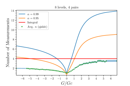
(a)

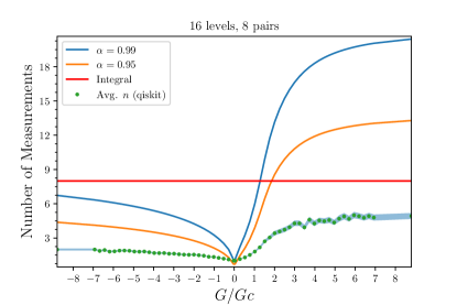
(b)

Figure 3: Estimated number of measurements, $n$, needed to get at least one observation with the correct particle number as a function of $G/G_{c}$ for the pairing Hamiltonian with $8$ (a) and $16$ (b) orbitals at half-filling. The red curve corresponds to the number of grid points to carry out number projection with gauge integration. The green dots are the average number for $n$ obtained experimentally from $10^{3}$ parallel runs on a noise-less quantum simulator (qiskit) along with their $95\%$ confidence intervals (shaded area). The blue and orange curves are theoretical upper bounds for $n$ with $\alpha=0.95,\;0.99$ computed from Eq. (22).

To compute expectation values over AGP, we need to implement the corresponding BCS wavefunction, correlated it, and perform post-selection at the end. To this end, it is crucial that we use a number conserving correlator, since

$$\hat{U}|\text{AGP}\rangle=\hat{U}\left(\mathcal{P}_{N}|\text{BCS}\rangle\right)=\mathcal{P}_{N}\hat{U}|\text{BCS}\rangle,$$ (21)

is true if and only if $[\mathcal{P}_{N},\hat{U}]=0$, where $\hat{U}$ is the correlator and $\mathcal{P}_{N}$ is the number projection operator. The disentangled uCC as described in Sec. II.3 satisfies this requirement.

In general, however, $\langle\text{BCS}|{\hat{N}}|\text{BCS}\rangle\neq 2N$, due to the broken $U(1)$ gauge degree of freedom in the BCS wavefunction Ring and Schuck (1980). This could lead to nonoptimal sampling during post-selection since we get samples that do not belong to the desired particle number sector on average. Fortunately, we can fix the gauge to $\langle{\hat{N}}\rangle=2N$ easily during the AGP optimization using projected BCS or NHFB by introducing a chemical potential. Doing so amounts to multiplying all $\eta_{p}$ by a constant number which does not change expectation values over AGP Khamoshi et al. (2019). Alternatively we can find this constant algebraically. See Appendix B.1.

A major advantage of using post-selection compared to gauge integration over the same Pauli set is the lack of an additional ancilla qubit needed to perform the Hadamard test, and the $\mathcal{O}(M)$ circuit depth for the controlled $R_{z}(\phi_{i})$ rotations. However, the difference in the scaling of number of measurements is more involved. For the integral, the number of measurements scales as $\mathcal{O}(M)$ corresponding to the total number of grid points, and it is independent of the Hamiltonian. To derive the scaling for post-selection, we formulate the problem as follows: What is the minimum number of measurements needed to get at least one observation in the correct number sector with $\alpha\times 100$ percent confidence? We show in Appendix B.2 that the number of measurements, $n$, is given by

$$n=\left\lceil\frac{\log(1-{\alpha})}{\log{(1-P)}}\right\rceil,$$ (22)

where $P={(\prod_{p}u_{p}^{2})}S_{N}^{M}$, and $S_{N}^{M}$ is an elementary symmetric polynomial associated with the norm of AGP Khamoshi et al. (2019). Clearly $n$ depends on the details of the Hamiltonian through $P$, which itself is a function of $\{\eta_{p}\}$. The largest value of $n$ occurs when number symmetry is strongly broken and all $\{\eta_{p}\}$ approach the same value. This is the worst case scenario for post-selection and, as we show in Appendix B.2, it is asymptotically bounded above by $\mathcal{O}(\sqrt{M})$. In regimes where number symmetry does not break, the scaling could be as low as $\mathcal{O}(1)$.

III.2 Numerical experiments

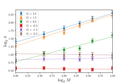
(a)

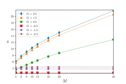
(b)

Figure 4: Scaling of post-selection as function of system size, $M$, for the pairing Hamiltonian. (a) The average number of measurements, $\bar{n}$, to get one observation with the correct particle number from repeated sampling on a quantum emulator (qiskit). The error bars correspond to the $95\%$ confidence intervals. This was performed for $M=4,6,8,10,12,16$ at different $G$ values. (b) The theoretical number of measurements on a linear scale computed from Eq. (22) with $\alpha=0.95$. This allows us to estimate $n$ for system much larger than those we can simulate on qiskit.

We put the scaling to numerical test by doing post-selection for the pairing Hamiltonian Ring and Schuck (1980); Dukelsky et al. (2004),

$$H =\sum_{p}\epsilon_{p}\mathbf{N}_{p}-G\sum_{pq}\mathbf{P}^{\dagger}_{p}\mathbf{P}_{q},$$ (23)

written here in the pairing algebra; $\epsilon_{p}=p\Delta\epsilon$ are the single particle energy levels and $G$ tunes the strength of the pair-wise interaction and has infinite range. The pairing model is an ideal benchmark as the mean-field breaks number symmetry—gives rise to a BCS state—at $G=G_{c}>0$ where number fluctuations get larger as $G$ increases; for all $G<G_{c}$ (including $G<0$) the mean-field admits a single HF Slater determinant for which the corresponding particle number fluctuations are small.

In Fig. (3) we plot $n$ computed from Eq. (22) with $\alpha=0.95$ and $0.99$ as a function of $G/G_{c}$ for $8$ and $16$ orbitals at half-filling. Half-filling is the ideal case for the integration as it requires the fewest number of grid points, whereas the opposite is true for post-selection. We also numerically simulated post-selection on qiskit noa (2019), using the QASM simulation libraries in the absence of noise. For every $G$ point, we simulated the BCS state and performed multiple measurements until we got an outcome with the correct particle number. This process was repeated $10^{3}$ to estimate $n$ by the empirical mean, $\bar{n}$. The $95\%$ confidence intervals were computed from bootstrapping the samples $10^{4}$ times and are shown with the shaded area in the plot. As we can see, the sample means along with their confidence intervals are below the number of measurements needed for the integral for all points, even in $G\gg G_{c}$ where number fluctuations are large. This suggests that number symmetry restoration with post-selection could be a viable alternative to gauge integration even in small systems with large number fluctuations.

In Fig. (4) we numerically investigate the scaling of post-selection as a function of system size $M$. On the left hand side of Fig. (4) we plot the sample means, $\bar{n}$, computed at different $G/G_{c}$ points on a log-log scale as a function of the system size $M$. Linear fits to the mean resulted in slopes: $m=0.449,0.488,0.392,-0.01,0.027,-0.02$ rounded to the closest digits in decreasing order of $G$. On the right side of the figure, we used Eq. (22) to compute $n$ beyond what we could simulate on qiskit, with system size as large as $M=40$. The results suggest $\mathcal{O}(1)$ scaling in $G<0$, where number symmetry does not break, and a $\mathcal{O}(\sqrt{M})$ where number symmetry breaks. This is inline with the $\mathcal{O}(\sqrt{M})$ asymptotic scaling found analytically and shown in detail in Appendix B.2.

In summary, Table 1 compares the scaling cost of phase estimation, exact gauge integration, and post-selection as methods to restore number symmetry. For phase estimation, one could follow Refs. McArdle et al. (2019); Lacroix (2020) and use our technique to guarantee an $\mathcal{O}(\sqrt{M})$ scaling for the number of measurements. If mid-circuit measurement is feasible on a quantum computer, then phase estimation can be carried out with only one ancilla qubit i.e. $\mathcal{O}(1)$ scaling instead of $\mathcal{O}(\log(M))$.

Method	Measurements	Depth	Ancilla qubits
Phase estimation	$\mathcal{O}(\sqrt{M})$	$\mathcal{O}(M\log(M))$	$\mathcal{O}(\log(M))$
Gauge integral	$\mathcal{O}(M)$	$\mathcal{O}(M)$	$\mathcal{O}(1)$
Post-selection	$\mathcal{O}(\sqrt{M})$	$\mathcal{O}(1)$	None

Table 1: Scaling of number symmetry restoration using different methods as a function of system size ($M$) for a given number–conserving Pauli fragment.

IV Application

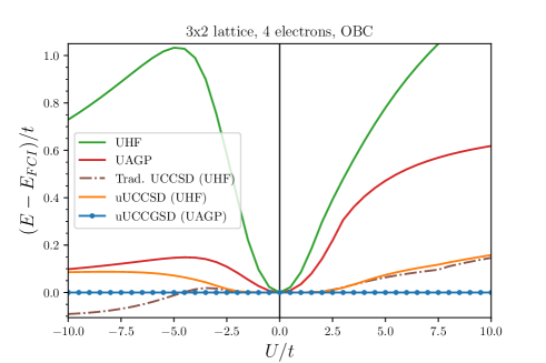
(a)

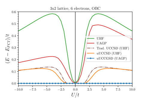
(b)

Figure 5: Energy error of fixed-reference calculations for 2D Hubbard with open boundary conditions (OBC) away from half-filling (a) and at half-filling (b) as a function of $U/t$. Traditional (Trad.) or disentangled unitary (u) spin-unrestricted coupled cluster calculations were performed based on UHF or UAGP references with single and double excitations (UCCSD) or their generalized coupled cluster counterpart (UCCGSD).

Having developed a method for how to optimize and implement AGP for quantum computers, we concentrate on building correlation atop of AGP for seniority nonzero applications in this section. Our aim is to showcase our method by benchmarking it against the ground state of the single-band Fermi–Hubbard model,

$$H=-t\sum_{\langle p,q\rangle}\sum_{\sigma\in\{\uparrow,\downarrow\}}\left({c}^{\dagger}_{p\sigma}{c}_{q\sigma}+h.c.\right)+U\sum_{p}n_{p\uparrow}n_{p\downarrow},$$ (24)

written here in its on-site basis, where $n_{p\sigma}={c}^{\dagger}_{p\sigma}{c}_{p\sigma}$. We set $t=1$ for simplicity for the rest of this section. For this Hamiltonian, number symmetry breaks at some finite $U<0$ value; and when $U>0$, the mean-filed breaks spin-symmetry at a critical $U>0$ . While one of the main advantages of using AGP is for models wherein the two-body interactions are attractive, we showcase our method in both the repulsive and attractive regimes of this Hamiltonian. Our strategy is to allow the $S^{2}$ symmetry to break (i.e. use UAGP) and correlate the resulting wavefunction. This helps us illustrate the utility of AGP in all regimes—attractive, repulsive, weak and strong limits. Indeed, to improve the results even more, one can envision restoring $S_{z}$ and/or $S^{2}$ which tend to break at sufficient strong correlation, but we leave those for future work.

We first present the results for the fixed-reference methods, wherein we have optimized UAGP on a classical computer and use quantum computers to optimize uCC atop of AGP. In the later half of this section, we demonstrate another powerful Ansatz based on a particle–hole unitary, which as we shall see, needs to be optimized simultaneously with the reference AGP.

The Implementation details of this section can be found in Appendix C.

IV.1 Fixed-reference

We implement our Ansätze with the following structure,

$$|{\psi}\rangle=\underbrace{\prod_{k}e^{\sigma_{k}}}_{\text{orbital rotation}}\underbrace{\left(\prod_{d}e^{\hat{D}_{d}}\right)}_{\text{doubles}}\underbrace{\left(\prod_{s}e^{\hat{S}_{s}}\right)}_{\text{singles}}|{\phi}\rangle,$$ (25)

where $|{\phi}\rangle$ can be AGP or HF. The orbital rotation is optional but it allows one to measure the Hamiltonian in the on-site basis which is significantly sparser and simpler than the natural orbital basis (see Sec. II.3). The on-site Hubbard Hamiltonian is also convenient for post-selection as it maps to

$$H=\frac{t}{2}\sum_{\langle p,q\rangle}\sum_{\sigma\in\{\uparrow,\downarrow\}}\left({X}_{p\sigma}{X}_{q\sigma}+{Y}_{p\sigma}{Y}_{q\sigma}\right)\prod_{n}{Z}_{n}\\ +\frac{U}{4}\sum_{p}\left(1-{Z}_{p\uparrow}\right)\left(1-{Z}_{p\downarrow}\right),$$ (26)

under the JW transformation. The only fragment that needs to be diagonalized is the nearest-neighbors hopping terms, for which we can apply the same circuit as the seniority-zero Hamiltonians shown in Fig. (2).

In Fig. (5) we show the VQE calculation results for the 2D Hubbard model at half-filling and away from half-filling with open boundary conditions (OBC). For the doped system, the number symmetry becomes strongly broken as $U<0$ get smaller. This is the kind of regime where we expect AGP-based methods to excel and traditional methods to struggle. Indeed, traditional UCCSD over-correlates in the 4-electron case as $U$ gets smaller and becomes difficult to converge starting near $U\approx-8$ up to some finite regime of $U$. In the $U>0$ regime of the same doped system, in addition to $S^{2}$, $S_{z}$ symmetry breaks at mean-field near $U\sim 7.5$; only the $S^{2}$ symmetry breaks for the half-filled case.

We plot uUCCGSD based on UAGP for all values of $U$. As a point of reference, we have plotted uUCCSD on UHF as well. The AGP-based results captured energies with absolute errors as small as $10^{-9}$ for both systems which is where we set the tolerance of our optimization. While this confirms that our AGP-based method is capable of accessing all relevant parts of the Hilbert space (not just seniority-zero for example) and get almost exact energies for these system, the high accuracy might be in part due its high number of variational parameters compared to the dimension of FCI. There are 870 variational parameters in uUCCGSD while the FCI dimension of the half-filled and doped systems are ${12\choose 6}=924$ and ${12\choose 4}=495$ respectively. We get equally good results with uUCCGSD on UHF for these systems. While this in principle can be tested by going to larger systems, our current implementation of the code allows for maximum system size of 12 spin-orbitals.

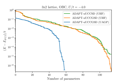
(a)

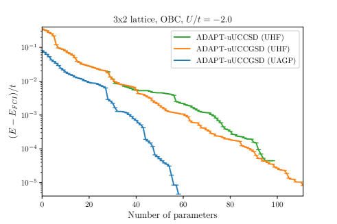
(b)

Figure 6: ADAPT-VQE calculations for HF- and AGP-based disentangled uCC (fixed-reference) for the 4 electron system at the strongly correlated point ($U/t=-4$) where mean-field methods struggle the most and a slightly less correlated point ($U/t=-2$) for comparison.

To find a sparser representation of the disentangled uUCCGSD we performed ADAPT-VQE Grimsley et al. (2019) calculations with the same operator pool as uUCCGSD for the 4-electron system. ADAPT-VQE was designed and tested for HF-based methods, but we follow the same idea for our implementation and use AGP as our reference. We set ADAPT’s stopping criterion to be $\epsilon=10^{-3}$. As shown in Fig. (6) energy errors of $10^{-6}$ were obtained with as few as 60 parameters with AGP. For comparison we also plotted particle–hole and general index HF-based calculations with the same computational settings. We observe the largest gains with AGP-based ADAPT in the regimes where number symmetry breaks and the system is strongly correlated. In large $U>0$, we did not see significant advantage in using AGP compared with HF. More studies are needed to tailor ADAPT for AGP-based methods. After submitting this paper, the recent work by Refs. Tsuchimochi et al. (2022); Bertels et al. (2022) has come to our attention in which the authors studied the affect of symmetry breaking in the ADAPT-VQE framework. While neither investigated the restoration of particle number symmetry, our results with AGP is complementary to their findings in that restoring symmetries that spontaneously break at the mean-field level could greatly benefit ADAPT’s convergence.

In the next section, we develope a particle–hole Ansatz on AGP which has considerably fewer parameters than uUCCGSD.

IV.2 Reference-optimized uCC

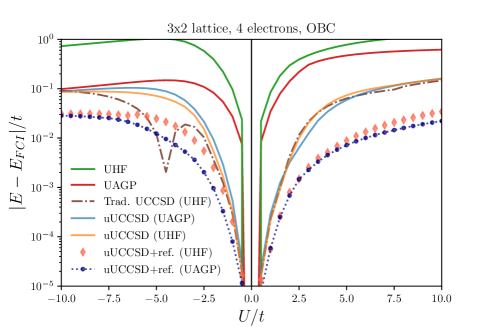
(a)

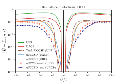
(b)

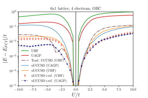
(c)

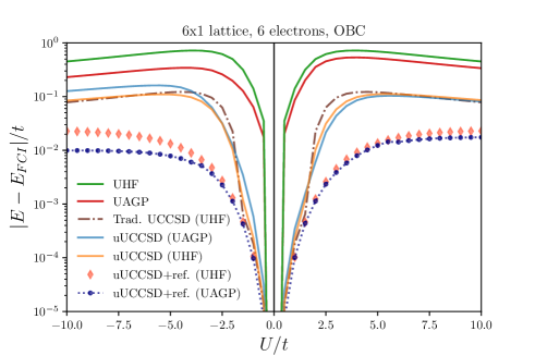
(d)

Figure 7: A particle–hole uCC Ansatz based on UAGP and UHF tested for one and two dimensional Hubbard model at and away from half-filling. Methods involving reference optimization are denoted by “+ref.”

One of the main advantages of using the uCC Ansatz with particle–hole excitations is that it is significantly more concise compared to one based on general operators. Ideally, we would like to develop a particle–hole uCC Ansatz based on AGP.

In general, the natural orbitals of AGP and HF are different. In the weakly correlated limit (e.g. $U\rightarrow 0$ for the Hubbard Hamiltonian), the HF and AGP orbitals converge to the same values and we get $\eta_{1},\cdots,\eta_{N}\rightarrow 1$ and $\eta_{N+1},\cdots,\eta_{M}\rightarrow 0$ (up to a global constat) so that AGP becomes just a single Slater determinant Dutta et al. (2020). For finite, nonzero $U$, we designate the first $N$ orbitals of the largest occupations as occupied and the rest virtual, thereby defining a “particle–hole” picture from which we can define our cluster operators. In our numerical experiments, particle–hole disentangled uCC makes only a small improvement on mean-field AGP in the attractive regime. However, we can remedy this by optimizing the AGP orbitals and geminal coefficients in the presence of the particle–hole correlator. As we shall see, we obtain significant improvement by so doing. Our observation is consistent with the results obtained in Ref. Baran and Dukelsky (2021) which was carried out for the pairing Hamiltonian.

Again, we implemented Eq. (25) for all of our Ansatz. However, instead of fixed orbital-rotation parameters, we optimized them simultaneously with uCC amplitudes. For AGP-based methods, we also optimized $\{\eta_{p}\}$ as discussed in Sec. II.2. Indeed, for HF, reference optimization corresponds to optimizing the orbitals only. For all cases, the Hamiltonian was measured in the on-site basis.

In Fig. (7) we show the results for the particle–hole uCC based on UAGP for 6 sites, 1- and 2-dimensions, with 4 and 6 electrons. We performed UHF-based calculations with the same optimization settings and Ansatz ordering as those for AGP. Just as in the fixed-reference case, we observed largest gains in the attractive regime. Nevertheless, our numerical results suggest that AGP can be just as competitive as HF in $U>0$ as a starting point for corrected method in all of the systems that we tried.

V Discussions

A desirable property for electronic structure methods is accurately describing the weakly and strongly correlated regimes seamlessly. One way to achieve this goal is to restore symmetries that break at the mean-field level as the result of strong correlation and capture the remaining correlation energy using CC-type correlators.

Building on our previous work that dealt with correlating AGP in the seniority-zero subspace, we developed a coupled cluster method to correlate AGP for general, seniority nonzero Hamiltonians on a quantum computer. We benchmarked our numerical results against the ground state of the Fermi–Hubbard Hamiltonian—a model Hamiltonian that breaks number symmetry when $U<0$ and breaks various spin-symmetries when $U>0$.

We proposed two techniques: First, we optimize AGP on a classical computer then correlate it on a quantum computer. We showed that uUCCGSD on AGP is highly accurate and capable of accessing all relevant parts of the Hilbert space. Using a naïve implementation of ADAPT-VQE on AGP in a 2-dimensional, doped Hubbard model, we observed that AGP-based uUCCGSD could give a sparser, yet highly accurate Ansatz in the regime where number symmetry breaks. Our second technique uses a particle–hole uCC based on AGP. The separation between particles and holes in AGP is not as well-defined as HF, and the orbitals are generally very different. However, by relaxing the reference in the presence of the particle–hole uCC correlator, we obtained excellent results in our numerical benchmarks.

In addition to correlating AGP, we illustrated how post-selection can fit well into our formalism to restore particle number. Symmetry restoration can be realized in a variety of ways on a quantum computer, including gauge integration and phase estimation. Post-selection relieves the need for implementing the Hadamard tests to evaluate the integral and is less expensive than phase estimation. Our main contribution is to show that the number of measurements in post-selection scales as $\mathcal{O}(\sqrt{M})$ in the worst case (where number is strongly-broken) in the absence of noise. We proved this analytically, and tested it numerically for the pairing Hamiltonian using a quantum emulator. Our numerical results suggest scaling of as low as $\mathcal{O}(1)$ in the regime where number symmetry does not break. In contrast, the measurement cost of exact gauge integration is $\mathcal{O}(M)$ and independent of the strength of the correlation.

Post-selection on particle number is often a necessary step for noise mitigation on NISQ hardware. However, when performed on an Ansatz that deliberately breaks number symmetry, one can recover additional correlation energy, even in the regimes that number symmetry does not break. This observation together with the fact that the cost of constructing disentangled uCC on AGP is the same as HF on a quantum computer, could make AGP an attractive wavefunction for the strong correlation. Future work could benefit from restoring spin-symmetries, such as $S^{2}$ and $S_{z}$ to further improve the accuracy of AGP-based methods for molecules. While issues related to the barren plateau problem McClean et al. (2018) are less prominent for physically inspired Ansätze , future work could also explore convergence properties of AGP-based uCC.

VI Acknowledgments

This work was supported by the U.S. Department of Energy under Award No. DE-SC0019374. G.E.S. is a Welch Foundation Chair (C-0036). A.K. is thankful to Garnet Kin-Lic Chan for insightful consultations on post-selection and thanks Jonathon P. Misiewicz amd Nicholas H. Stair for helpful inputs regarding QForte. G.P.C thanks Carlos A. Jimenez-Hoyos for discussions regarding NHFB and its implementation. A.K. and G.P.C are grateful to Thomas M. Henderson for helpful discussions.

Appendix

Appendix A Bloch–Messiah decomposition

An HFB state is defined as the vacuum of Bogoliubov quasiparticles,

$$|{\text{HFB}}\rangle=\prod_{p=1}^{2M}\beta_{p}|\text{vac}\rangle,$$ (27)

where the quasiparticle operators $\beta_{p}$, $\beta^{\dagger}_{p}$ are defined by a unitary canonical transformation $\mathcal{W}$ of the physical fermionic operators $c_{p}$, $c^{\dagger}_{p}$,

$$\begin{pmatrix}\beta\\ \beta^{\dagger}\end{pmatrix}=\mathcal{W}^{\dagger}\begin{pmatrix}c\\ c^{\dagger}\end{pmatrix}=\begin{pmatrix}U^{\dagger}&V^{\dagger}\\ V^{T}&U^{T}\end{pmatrix}\begin{pmatrix}c\\ c^{\dagger}\end{pmatrix},$$ (28)

wherein $U$ and $V$ are known as the Bogoliubov coefficients. By the Bloch–Messiah decomposition, we can bring $U$ and $V$ into a canonical form, which enables us to write the HFB as a BCS wavefunction in the natural orbital basis. As a consequence, a NHFB state optimized on a classical computer can be used to prepare an AGP on a quantum computer.

A.1 Bloch–Messiah theorem

The Bloch–Messiah theorem states that $\mathcal{W}$ can be decomposed into three unitary canonical transformations of special forms,

$$\mathcal{W}=\begin{pmatrix}U&V^{*}\\ V&U^{*}\end{pmatrix}=\begin{pmatrix}D&0\\ 0&D^{*}\end{pmatrix}\begin{pmatrix}\bar{U}&\bar{V}\\ \bar{V}&\bar{U}\end{pmatrix}\begin{pmatrix}C&0\\ 0&C^{*}\end{pmatrix},$$ (29)

where $D$ and $C$ are unitary matrices and

$$\bar{U} =\bigoplus_{p=1}^{M}\begin{pmatrix}u_{p}&0\\ 0&u_{p}\end{pmatrix},$$ (30a)

$$\bar{V} =\bigoplus_{p=1}^{M}\begin{pmatrix}0&v_{p}\\ -v_{p}&0\end{pmatrix},$$ (30b)

are real matrices whose nonzero elements are BCS coefficients $\{u_{p},v_{p}\}$. $D$ is called the canonical orbital coefficients and is identical to the natural orbital coefficients of the geminal defined in Eq. (6), hence the same symbol. This can be readily seen by recognizing $\eta=(VU^{-1})^{*}$ and $\bar{\eta}=(\bar{V}\bar{U}^{-1})^{*}$. Incidentally, the most general form of the Bloch–Messiah theorem applies to both odd and even electron systems, albeit we restrict ourselves to even electron systems herein.

A.2 Computing Bloch–Messiah decomposition

Given an HFB, we denote its one-particle reduce density matrix by $\rho$ and pairing matrix by $\kappa$. $\rho$ is Hermitian and $\kappa$ antisymmetric. They relate to the Bogoliubov coefficients through Ring and Schuck (1980)

$$\rho =V^{*}V^{T},$$ (31a)

$$\kappa =V^{*}U^{T},$$ (31b)

and thus satisfy

$$\rho\kappa =\kappa\rho^{*},$$ (32a)

$$\rho-\rho^{2} =\kappa\kappa^{\dagger}.$$ (32b)

Computing the Bloch–Messiah decomposition amounts to simultaneously diagonalizing $\rho$ and canonicalizing $\kappa$ Hua (1944) in the sense of

$$\bar{\rho} =\bigoplus_{p=1}^{M}\begin{pmatrix}\rho_{p}&0\\ 0&\rho_{p}\end{pmatrix}=D^{\dagger}\rho D,$$ (33a)

$$\bar{\kappa} =\bigoplus_{p=1}^{M}\begin{pmatrix}0&\kappa_{p}\\ -\kappa_{p}&0\end{pmatrix}=D^{\dagger}\kappa D^{*},$$ (33b)

where $\bar{\rho}$ and $\bar{\kappa}$ are real. To do this, we just need to canonicalize $\kappa$ in each degenerate eigen subspace of $\rho$. Canonicalization of an antisymmetric matrix can be performed using algorithms described in Wimmer (2012). Subsequently, $\{u_{p},v_{p}\}$, or equivalently $\{\eta_{p}\}$, can be determined from the values of $\{\rho_{p},\kappa_{p}\}$.

Specifically for UHFB, $\rho$ and $\kappa$ have the following spin block structures:

$$\rho =\begin{pmatrix}\rho^{\alpha\alpha}&0\\ 0&\rho^{\beta\beta}\end{pmatrix},$$ (34a)

$$\kappa =\begin{pmatrix}0&\kappa^{\alpha\beta}\\ -(\kappa^{\alpha\beta})^{T}&0\end{pmatrix}.$$ (34b)

By Eq. (32), we have

$$\left[\rho^{\alpha\alpha},\>\kappa^{\alpha\beta}\left(\kappa^{\alpha\beta}\right)^{\dagger}\right] =0,$$ (35a)

$$\left[\rho^{\beta\beta},\>\left(\kappa^{\alpha\beta}\right)^{T}\kappa^{\alpha\beta*}\right] =0,$$ (35b)

which implies that we can simultaneously diagonalize the Hermitian matrices $\rho^{\alpha\alpha}$, $\rho^{\beta\beta}$, and $\kappa^{\alpha\beta}\left(\kappa^{\alpha\beta}\right)^{\dagger}$. We can show that the eigenvalues of $\rho^{\alpha\alpha}$ are identical to those of $\rho^{\beta\beta}$. Moreover, we can always find unitary matrices $D^{\alpha}$ and $D^{\beta}$ such that the columns of $D^{\alpha}$ are the eigenvectors of $\rho^{\alpha\alpha}$ and the left singular vectors of $\kappa^{\alpha\beta}$, while the columns of $D^{\beta}$ are the eigenvectors of $\rho^{\beta\beta}$ and the complex conjugate of the right singular vectors of $\kappa^{\alpha\beta}$. The matrix of canonical orbital coefficients is then written as

$$D=\begin{pmatrix}D^{\alpha}&0\\ 0&D^{\beta}\end{pmatrix}P^{T},$$ (36)

where $P$ is the permutation matrix of

$$\begin{pmatrix}1&2&\cdots&M&M+1&M+2&\cdots&2M\\ 1&3&\cdots&2M-1&2&4&\cdots&2M\end{pmatrix}.$$ (37)

This permutation arises because we choose to put the paired spin-orbitals $p$ and $\bar{p}$ adjacent to each other in Eq. (30). We see from Eq. (36) that a $(p,\,\bar{p})$ pair in UHFB is a spin pair. Consequently, the natural orbital pairs in UAGP are spin pairs.

We can carry out a similar procedure to find the canonical orbital coefficients $D$ and thereby the Bloch–Messiah decomposition for RHFB. In this case, $D$ is in the form of Eq. (36) with $D^{\alpha}=D^{\beta}$.

Appendix B Post-selection analysis

B.1 Fixing the gauge

As evident from Eq. (4), multiplying all $\{\eta_{p}\}$ by a constant, $c$, amounts to multiplying AGP by an inconsequential global constant $c^{N}$. The same however is not true for the BCS wavefunction, since a global constant cannot be factorized. In BCS, multiplying all $\eta_{p}$ changes the average particle number. Therefore, given a set of $\eta_{p}$, we can solve for $c$ so that the average particle number is fixed. Recall that,

$$\langle\text{BCS}|{\hat{N}}|\text{BCS}\rangle=\sum_{p=1}^{M}2{v_{p}^{2}}=2\sum_{p=1}^{M}\frac{{\eta_{p}^{2}}}{1+{\eta_{p}^{2}}},$$ (38)

where we used the fact that $\eta_{p}=v_{p}/u_{p}$ and ${u_{p}^{2}}+{v_{p}^{2}}=1$ in the last equality. We need, $\langle{\hat{N}}\rangle=2N$, so we can solve for $c$ (it can be taken to be real) that satisfies,

$$\sum_{p}\frac{(c\eta_{p})^{2}}{1+(c\eta_{p})^{2}}-N=0.$$ (39)

We are not aware of a simple closed-form solution. However, it is easy to solve for $c$ numerically with standard root finding algorithms. This can be particularly helpful when optimizing the reference AGP on a quantum computer such as Sec. IV.2 or Sec. II.2, where for every guess of $\{\eta_{p}\}$, they can be scaled to maximize sampling outcomes.

B.2 Scaling of post-selection

We want show that the asymptotic scaling of post-selection is no worse that $\mathcal{O}(\sqrt{M})$. To this end, we first derive an analytical expression for the number of measurements needed to obtain at least one sample in the correct particle number sector. We then find an upper bound to this expression which gives us the asymptotic scaling.

Typically, we are interested in computing the expectation value of some observable $\hat{O}$ over correlated AGP. we concentrate on number conserving operators, since otherwise their expectation values over AGP are zero. Let $\hat{U}$ define a number conserving correlator so that $[\mathcal{P}_{N},\hat{U}]=0$. We want to compute

$$\frac{\langle\text{AGP}|{\hat{U}^{\dagger}\hat{O}\hat{U}}|\text{AGP}\rangle}{\langle\text{AGP}|\text{AGP}\rangle}=\sum_{\alpha}\lambda_{\alpha}\frac{|\langle{\lambda_{\alpha}}|\hat{V}\hat{U}|\text{AGP}\rangle|^{2}}{\langle\text{AGP}|\text{AGP}\rangle},$$ (40)

where $\hat{V}$ diagonalizes $\hat{O}$, (i.e. $\hat{O}=\hat{V}^{\dagger}{\hat{\Lambda}}\hat{V}$) and $|{\lambda_{\alpha}}\rangle$ is a bit string corresponding to eigenvector of ${\hat{\Lambda}}$ with eigenvalue $\lambda_{\alpha}$. In practice, we need to compute Eq. (40) using the projected BCS wavefunction. Therefore we have

$$|\langle{\lambda_{\alpha}}|\mathcal{P}_{N}\hat{V}\hat{U}|\text{BCS}\rangle|^{2}=|\langle{\lambda_{\alpha}}|\hat{V}\hat{U}\mathcal{P}_{N}|\text{BCS}\rangle|^{2}$$

$$=\underbrace{\frac{|\langle{\lambda_{\alpha}}|\hat{V}\hat{U}|\text{AGP}\rangle|^{2}}{\langle\text{AGP}|\text{AGP}\rangle}}_{P(\lambda_{\alpha}|N)}\underbrace{\frac{|\langle\text{AGP}|\text{BCS}\rangle|^{2}}{\langle\text{AGP}|\text{AGP}\rangle}}_{P(N)},$$ (41)

where $P(N)$ is the probability of getting a state with $N$ pairs and $P(\lambda_{\alpha}|N)$ is the probability of getting $\lambda_{\alpha}$ conditioned on $N$. This shows that, the scaling of post-selection is solely determined by $P(N)$ and is independent of the operator $\hat{O}$ and the correlator $\hat{U}$ so long as they are number conserving.

From Eq. (B.2) we have

$$P(N)=\prod_{p}{u_{p}^{2}}\langle\text{AGP}|\text{AGP}\rangle,$$ (42)

where $\langle\text{AGP}|\text{AGP}\rangle=\sum_{1\leq p_{1}<\cdots<p_{N}\leq M}{\eta_{p_{1}}^{2}}\cdots{\eta_{p_{N}}^{2}}^{=}S_{N}^{M}$ is an elementary symmetric polynomial (ESP) Khamoshi et al. (2019). If we did $n$ independent measurements, the probability of getting $k$ observations in the desired particle sector (in the absence of noise) follows a Binomial distribution,

$${P(k;n)}={n\choose k}P^{k}(1-P)^{n-k},$$ (43)

where $P$ is a shorthand notation for $P(N)$. Therefore, it follows that

$$P(k\geq 1)=\alpha\implies n=\frac{\log(1-{\alpha})}{\log{(1-P)}}.$$ (44)

rounded to the closest integer (ceiling). For example, if we want to be 95% confident that there is at least one observation in the desired particle sector, we need a sample size of $n=\lceil{-2.996}/{\log{(1-P)}}\rceil$, where $P$ needs to be computed numerically from Eq. (42).

Finding an upper bound for $n$ is equivalent to bounding $P$ from below. The precise value of $P$ depends on a given Hamiltonian and varies at different correlation regimes; except for special cases, an analytic expressions for $P$ is not known. However, since $0<P<1$ we can look at its limiting cases to find the lower and upper bounds.

As $P\rightarrow 1$, we get $n\rightarrow 1$, which corresponds to the HF limit of AGP where fluctuations in particle number are minimal. Indeed this is the upper bound to $P$. The lower limit corresponds to the opposite case where number symmetry is strongly broken and the number fluctuations are at their peak. Physically, this is associated with the superfluid phase where the occupation number of all orbitals become equal. In this case—assuming $\{\eta_{p}\}$ normalized so that $\langle\text{BCS}|{\hat{N}}|\text{BCS}\rangle=2N$ (vide supra)—we get

$$v_{p}^{2}=\frac{N}{M},\quad u_{p}^{2}=\frac{M-N}{M},$$ (45a)

$$\eta_{p}^{2}=\frac{N}{M-N}.$$ (45b)

The lower-bound of $P$ can be obtained by plugging these expressions into Eq. (42), so we arrive at

$$P=\frac{N^{N}(M-N)^{M-N}}{M^{M}}{M\choose N}.$$ (46)

Using Stirling’s approximation,

$${M\choose N}\sim{M^{M}\over N^{N}(M-N)^{M-N}}\sqrt{M\over 2\pi N(M-N)},$$ (47)

we get

$$P\approx\sqrt{M\over 2\pi N(M-N)}.$$ (48)

Let $\xi=N/M$ define an intensive quantity. We may assume $\xi\leq 1/2$ for all practical purposes. Simplifying $P$ gives

$$P \approx\frac{1}{\sqrt{2\pi M\xi(1-\xi)}}\geq\frac{1}{\sqrt{\pi M/2}}.$$ (49)

Finally, to get the asymptotic scaling for $n$, we Taylor expand near $P\rightarrow 0$,

$$n\propto\frac{1}{-\log{(1-P)}}=\frac{1}{P}-\frac{1}{2}-\frac{P}{12}+\mathcal{O}(P^{2}),$$ (50)

and plug in Eq. (49) to obtain

$$n \propto\sqrt{\frac{\pi M}{2}}+\mathcal{O}(P).$$ (51)

This finishes the proof as it shows $n\sim\mathcal{O}(\sqrt{M})$

Appendix C Implementation details

In Sec. IV, we used PySCF Sun et al. (2018) to carry out all UHF and traditional UCCSD calculations. Our quantum algorithms were implemented using the QForte Stair and Evangelista (2022) software with the “state-vector” emulator in the absence of noise. We made slight modifications to QForte libraries to implement AGP and orbital rotation/optimization in an in-house code. For the fixed-reference UHF-based calculations, we obtained the molecular orbital coefficients from PySCF; for AGP-based calculations, we used an in-house NHFB code.

For computational feasibility of our quantum algorithms, we implemented AGP by brute force; we looped over all states in the Hilbert space and assigned appropriate coefficients to each state. The procedure can be more easily seen if we expand Eq. (4) to get

$$|\text{AGP}\rangle=\sum_{1\leq p_{1}<\cdots<p_{N}\leq M}\eta_{p_{1}}\cdots\eta_{p_{N}}\mathbf{P}^{\dagger}_{p_{1}}\cdots\mathbf{P}^{\dagger}_{p_{N}}|\text{vac}\rangle.$$ (52)

For example, for the $M=4$, $N=2$ state, we have

$$|\text{AGP}\rangle =$$

$${}\eta_{1}\eta_{2}|{00001111}\rangle+\eta_{1}\eta_{3}|{00110011}\rangle$$

$$+ {}\eta_{1}\eta_{4}|{11000011}\rangle+\eta_{2}\eta_{3}|{00111100}\rangle$$

$$+ {}\eta_{2}\eta_{4}|{11001100}\rangle+\eta_{3}\eta_{4}|{11110000}\rangle,$$ (53)

Note that this state is not normalized, i.e. $\langle\text{AGP}|\text{AGP}\rangle\neq 1$; it is necessary to divide all energy and gradient expressions with appropriate normalization. The gradient with respect to $\eta_{p}$ can be computed from Khamoshi et al. (2019)

$$\frac{d}{d\eta_{p}}|\text{AGP}\rangle=\frac{1}{2\eta_{p}}\mathbf{N}_{p}|\text{AGP}\rangle.$$ (54)

On a quantum computer, however, we can efficiently compute the gradient by applying the shift-rule to the parameters of the unitary that implements the BCS wavefunction and number projecting the resulting term. This follows from the fact that $\left[\frac{d}{d\eta_{p}},\mathcal{P}_{N}\right]=0$.

We relied on the existing implementation for ADAPT and VQE calculations which use the SciPy libraries Virtanen et al. (2020) to do the intermediate optimizations. We set the optimizer to be L-BFGS-B Byrd et al. (1995); the gradients threshold as well as the energy difference tolerance were set to $10^{-9}$. In ADAPT, there is an additional tolerance, $\epsilon$, that determines when it terminates; we set $\epsilon=10^{-3}$ for the results shown in Fig. (6). In all calculations, the gradients were computed analytically.

To implement orbital rotation, we used an in-house code to perform a QR decomposition in terms of Givens rotations; we followed the work of Ref. Kivlichan et al. (2018) closely and implemented the rotations in QForte using 1-body rotations acting on nearest neighbors. For the orbital optimization of Sec. IV.2 we treated each of these 1-body rotations as independent parameters. Note that care must be given in making sure spin symmetries are retained. In all of our calculation with orbital optimization, we made certain that $S_{z}$ does not break—hence UAGP and UHF—by construction.

References

- Cao et al. (2019) Y. Cao, J. Romero, J. P. Olson, M. Degroote, P. D. Johnson, M. Kieferová, I. D. Kivlichan, T. Menke, B. Peropadre, N. P. D. Sawaya, S. Sim, L. Veis, and A. Aspuru-Guzik, Chem. Rev. 119, 10856 (2019).
- McArdle et al. (2020) S. McArdle, S. Endo, A. Aspuru-Guzik, S. C. Benjamin, and X. Yuan, Rev. Mod. Phys. 92, 015003 (2020).
- Helgaker et al. (2000) T. Helgaker, P. Jørgensen, and J. Olsen, Molecular electronic-structure theory (Wiley, Chichester; New York, 2000).
- Scuseria et al. (1987) G. E. Scuseria, A. C. Scheiner, T. J. Lee, J. E. Rice, and H. F. Schaefer, J. Chem. Phys. 86, 2881 (1987).
- Bartlett and Musiał (2007) R. J. Bartlett and M. Musiał, Rev. Mod. Phys. 79, 291 (2007).
- Bulik et al. (2015) I. W. Bulik, T. M. Henderson, and G. E. Scuseria, J. Chem. Theory Comput. 11, 3171 (2015).
- Ring and Schuck (1980) P. Ring and P. Schuck, The Nuclear Many-Body Problem, Theoretical and Mathematical Physics, The Nuclear Many-Body Problem (Springer-Verlag, Berlin Heidelberg, 1980).
- Blaizot and Ripka (1986) J.-P. Blaizot and G. Ripka, Quantum theory of finite systems (MIT Press, Cambridge, Mass., 1986).
- Löwdin (1955) P.-O. Löwdin, Phys. Rev. 97, 1509 (1955).
- Lykos and Pratt (1963) P. Lykos and G. W. Pratt, Rev. Mod. Phys. 35, 496 (1963).
- Scuseria et al. (2011) G. E. Scuseria, C. A. Jiménez-Hoyos, T. M. Henderson, K. Samanta, and J. K. Ellis, J. Chem. Phys. 135, 124108 (2011).
- Jiménez-Hoyos et al. (2012) C. A. Jiménez-Hoyos, T. M. Henderson, T. Tsuchimochi, and G. E. Scuseria, J. Chem. Phys. 136, 164109 (2012).
- Evangelista (2011) F. A. Evangelista, J. Chem. Phys. 134, 224102 (2011).
- Duguet (2015) T. Duguet, J. Phys. G: Nucl. Part. Phys. 42, 025107 (2015).
- Qiu et al. (2017) Y. Qiu, T. M. Henderson, J. Zhao, and G. E. Scuseria, J. Chem. Phys. 147, 064111 (2017).
- Cerezo et al. (2021) M. Cerezo, A. Arrasmith, R. Babbush, S. C. Benjamin, S. Endo, K. Fujii, J. R. McClean, K. Mitarai, X. Yuan, L. Cincio, and P. J. Coles, Nat. Rev. Phys. 3, 625 (2021).
- Shen et al. (2017) Y. Shen, X. Zhang, S. Zhang, J.-N. Zhang, M.-H. Yung, and K. Kim, Phys. Rev. A 95, 020501 (2017).
- Tilly et al. (2021) J. Tilly, H. Chen, S. Cao, D. Picozzi, K. Setia, Y. Li, E. Grant, L. Wossnig, I. Rungger, G. H. Booth, and J. Tennyson, arXiv:2111.05176 [quant-ph] (2021).
- Anand et al. (2022) A. Anand, P. Schleich, S. Alperin-Lea, P. W. K. Jensen, S. Sim, M. Díaz-Tinoco, J. S. Kottmann, M. Degroote, A. F. Izmaylov, and A. Aspuru-Guzik, Chem. Soc. Rev. 51, 1659 (2022).
- Evangelista et al. (2019) F. A. Evangelista, G. K.-L. Chan, and G. E. Scuseria, J. Chem. Phys. 151, 244112 (2019).
- Grimsley et al. (2020) H. R. Grimsley, D. Claudino, S. E. Economou, E. Barnes, and N. J. Mayhall, J. Chem. Theory Comput. 16, 1 (2020).
- Izmaylov et al. (2020a) A. F. Izmaylov, M. Díaz-Tinoco, and R. A. Lang, Phys. Chem. Chem. Phys. 22, 12980 (2020a).
- Peruzzo et al. (2014) A. Peruzzo, J. McClean, P. Shadbolt, M.-H. Yung, X.-Q. Zhou, P. J. Love, A. Aspuru-Guzik, and J. L. O’Brien, Nat. Commun. 5, 1 (2014).
- McClean et al. (2016) J. R. McClean, J. Romero, R. Babbush, and A. Aspuru-Guzik, New J. Phys. 18, 023023 (2016).
- Grimsley et al. (2019) H. R. Grimsley, S. E. Economou, E. Barnes, and N. J. Mayhall, Nat. Commun. 10, 3007 (2019).
- Tang et al. (2021) H. L. Tang, V. Shkolnikov, G. S. Barron, H. R. Grimsley, N. J. Mayhall, E. Barnes, and S. E. Economou, PRX Quantum 2, 020310 (2021).
- Grimsley et al. (2022) H. R. Grimsley, G. S. Barron, E. Barnes, S. E. Economou, and N. J. Mayhall, (2022), 10.48550/ARXIV.2204.07179.
- Romero et al. (2022) A. M. Romero, J. Engel, H. L. Tang, and S. E. Economou, Phys. Rev. C 105, 064317 (2022).
- Ryabinkin et al. (2018) I. G. Ryabinkin, T.-C. Yen, S. N. Genin, and A. F. Izmaylov, J. Chem. Theory Comput. 14, 6317 (2018).
- Ryabinkin et al. (2020) I. G. Ryabinkin, R. A. Lang, S. N. Genin, and A. F. Izmaylov, J. Chem. Theory Comput. 16, 1055 (2020).
- Matsuzawa and Kurashige (2020) Y. Matsuzawa and Y. Kurashige, J. Chem. Theory Comput. 16, 944 (2020).
- Lee et al. (2019) J. Lee, W. J. Huggins, M. Head-Gordon, and K. B. Whaley, J. Chem. Theory Comput. 15, 311 (2019).
- Stair and Evangelista (2021) N. H. Stair and F. A. Evangelista, PRX Quantum 2, 030301 (2021).
- Kandala et al. (2017) A. Kandala, A. Mezzacapo, K. Temme, M. Takita, M. Brink, J. M. Chow, and J. M. Gambetta, Nature 549, 242 (2017).
- Dallaire-Demers et al. (2019) P.-L. Dallaire-Demers, J. Romero, L. Veis, S. Sim, and A. Aspuru-Guzik, Quantum Sci. Technol. 4, 045005 (2019).
- Xia and Kais (2020) R. Xia and S. Kais, Quantum Sci. Technol. 6, 015001 (2020).
- Anselmetti et al. (2021) G.-L. R. Anselmetti, D. Wierichs, C. Gogolin, and R. M. Parrish, New J. Phys. 23, 113010 (2021).
- Huggins et al. (2022) W. J. Huggins, B. A. O’Gorman, N. C. Rubin, D. R. Reichman, R. Babbush, and J. Lee, Nature 603, 416 (2022).
- Preskill (2018) J. Preskill, Quantum 2, 79 (2018).
- Leymann and Barzen (2020) F. Leymann and J. Barzen, Quantum Sci. Technol. 5, 044007 (2020).
- Duguet and Signoracci (2017) T. Duguet and A. Signoracci, J. Phys. G: Nucl. Part. Phys. 44, 015103 (2017).
- Wahlen-Strothman et al. (2017) J. M. Wahlen-Strothman, T. M. Henderson, M. R. Hermes, M. Degroote, Y. Qiu, J. Zhao, J. Dukelsky, and G. E. Scuseria, The Journal of Chemical Physics 146, 054110 (2017).
- Qiu et al. (2019) Y. Qiu, T. M. Henderson, T. Duguet, and G. E. Scuseria, Phys. Rev. C 99, 044301 (2019).
- Song et al. (2022) R. Song, T. M. Henderson, and G. E. Scuseria, J. Chem. Phys. 156, 104105 (2022).
- Sheikh et al. (2021) J. A. Sheikh, J. Dobaczewski, P. Ring, L. M. Robledo, and C. Yannouleas, J. Phys. G: Nucl. Part. Phys. 48, 123001 (2021).
- Izmaylov (2019) A. F. Izmaylov, J. Phys. Chem. A 123, 3429 (2019).
- Yen et al. (2019) T.-C. Yen, R. A. Lang, and A. F. Izmaylov, J. Chem. Phys. 151, 164111 (2019).
- Tsuchimochi et al. (2020) T. Tsuchimochi, Y. Mori, and S. L. Ten-no, Phys. Rev. Research 2, 043142 (2020).
- Seki et al. (2020) K. Seki, T. Shirakawa, and S. Yunoki, Phys. Rev. A 101, 052340 (2020).
- Lacroix (2020) D. Lacroix, Phys. Rev. Lett. 125, 230502 (2020).
- Siwach and Lacroix (2021) P. Siwach and D. Lacroix, Phys. Rev. A 104, 062435 (2021).
- Seki and Yunoki (2022) K. Seki and S. Yunoki, Phys. Rev. A 105, 032419 (2022).
- Ruiz Guzman and Lacroix (2022) E. A. Ruiz Guzman and D. Lacroix, Phys. Rev. C 105, 024324 (2022).
- Khamoshi et al. (2020) A. Khamoshi, F. A. Evangelista, and G. E. Scuseria, Quantum Sci. Technol. 6, 014004 (2020).
- Yang (1962) C. N. Yang, Rev. Mod. Phys. 34, 694 (1962).
- Coleman (1965) A. J. Coleman, J. Math. Phys. 6, 1425 (1965).
- Sager and Mazziotti (2022) L. M. Sager and D. A. Mazziotti, Phys. Rev. Research 4, 013003 (2022).
- Bardeen et al. (1957) J. Bardeen, L. N. Cooper, and J. R. Schrieffer, Phys. Rev. 108, 1175 (1957).
- Brink and Broglia (2005) D. M. Brink and R. A. Broglia, Nuclear Superfluidity: Pairing in Finite Systems, 1st ed. (Cambridge University Press, 2005).
- Sedrakian and Clark (2019) A. Sedrakian and J. W. Clark, Eur. Phys. J. A 55, 167 (2019).
- Bach et al. (1994) V. Bach, E. H. Lieb, and J. P. Solovej, J Stat Phys 76, 3 (1994).
- Surján (1999) P. R. Surján, Top. Curr. Chem. 203, 63 (1999).
- Henderson and Scuseria (2019) T. M. Henderson and G. E. Scuseria, J. Chem. Phys. 151, 051101 (2019).
- Khamoshi et al. (2019) A. Khamoshi, T. M. Henderson, and G. E. Scuseria, J. Chem. Phys. 151, 184103 (2019).
- Dutta et al. (2020) R. Dutta, T. M. Henderson, and G. E. Scuseria, J. Chem. Theory Comput. 16, 6358 (2020).
- Henderson and Scuseria (2020) T. M. Henderson and G. E. Scuseria, J. Chem. Phys. 153, 084111 (2020).
- Dutta et al. (2021) R. Dutta, G. P. Chen, T. M. Henderson, and G. E. Scuseria, J. Chem. Phys. 154, 114112 (2021).
- Khamoshi et al. (2021) A. Khamoshi, G. P. Chen, T. M. Henderson, and G. E. Scuseria, J. Chem. Phys. 154, 074113 (2021).
- Casula and Sorella (2003) M. Casula and S. Sorella, J. Chem. Phys. 119, 6500 (2003).
- Casula et al. (2004) M. Casula, C. Attaccalite, and S. Sorella, J. Chem. Phys. 121, 7110 (2004).
- Wei and Neuscamman (2018) H. Wei and E. Neuscamman, J. Chem. Phys. 149, 184106 (2018).
- Genovese et al. (2019) C. Genovese, A. Meninno, and S. Sorella, J. Chem. Phys. 150, 084102 (2019).
- Genovese and Sorella (2020) C. Genovese and S. Sorella, J. Chem. Phys. 153, 164301 (2020).
- Neuscamman (2013a) E. Neuscamman, J. Chem. Phys. 139, 194105 (2013a).
- Neuscamman (2013b) E. Neuscamman, J. Chem. Phys. 139, 181101 (2013b).
- Fecteau et al. (2020a) C.-E. Fecteau, F. Berthiaume, M. Khalfoun, and P. A. Johnson, J. Math. Chem. (2020a).
- Johnson et al. (2020) P. A. Johnson, C.-E. Fecteau, F. Berthiaume, S. Cloutier, L. Carrier, M. Gratton, P. Bultinck, S. De Baerdemacker, D. Van Neck, P. Limacher, and P. W. Ayers, J. Chem. Phys. 153, 104110 (2020).
- Johnson et al. (2021) P. A. Johnson, H. Fortin, S. Cloutier, and C.-É. Fecteau, J. Chem. Phys. 154, 124125 (2021).
- Fecteau et al. (2020b) C.-E. Fecteau, H. Fortin, S. Cloutier, and P. A. Johnson, J. Chem. Phys. 153, 164117 (2020b).
- Fecteau et al. (2022) C.-É. Fecteau, S. Cloutier, J.-D. Moisset, J. Boulay, P. Bultinck, A. Faribault, and P. A. Johnson, J. Chem. Phys. 156, 194103 (2022).
- Moisset et al. (2022) J.-D. Moisset, C.-É. Fecteau, and P. A. Johnson, J. Chem. Phys. 156, 214110 (2022).
- Endo et al. (2018) S. Endo, S. C. Benjamin, and Y. Li, Phys. Rev. X 8, 031027 (2018).
- Bonet-Monroig et al. (2018) X. Bonet-Monroig, R. Sagastizabal, M. Singh, and T. E. O’Brien, Phys. Rev. A 98, 062339 (2018).
- Kandala et al. (2019) A. Kandala, K. Temme, A. D. Córcoles, A. Mezzacapo, J. M. Chow, and J. M. Gambetta, Nature 567, 491 (2019).
- Endo et al. (2021) S. Endo, Z. Cai, S. C. Benjamin, and X. Yuan, J. Phys. Soc. Jpn. 90, 032001 (2021).
- Huggins et al. (2021) W. J. Huggins, J. R. McClean, N. C. Rubin, Z. Jiang, N. Wiebe, K. B. Whaley, and R. Babbush, npj Quantum Inf 7, 23 (2021).
- Hua (1944) L.-K. Hua, Am. J. Math. 66, 470 (1944).
- Henderson et al. (2015) T. M. Henderson, I. W. Bulik, and G. E. Scuseria, J. Chem. Phys. 142, 214116 (2015).
- Bytautas et al. (2011) L. Bytautas, T. M. Henderson, C. A. Jiménez-Hoyos, J. K. Ellis, and G. E. Scuseria, J. Chem. Phys. 135, 044119 (2011).
- Stein et al. (2014) T. Stein, T. M. Henderson, and G. E. Scuseria, J. Chem. Phys. 140, 214113 (2014).
- Henderson et al. (2014) T. M. Henderson, I. W. Bulik, T. Stein, and G. E. Scuseria, J. Chem. Phys. 141, 244104 (2014).
- Bytautas et al. (2015) L. Bytautas, G. E. Scuseria, and K. Ruedenberg, J. Chem. Phys. 143, 094105 (2015).
- Shepherd et al. (2016) J. J. Shepherd, T. M. Henderson, and G. E. Scuseria, J. Chem. Phys. 144, 094112 (2016).
- Elfving et al. (2021) V. E. Elfving, M. Millaruelo, J. A. Gámez, and C. Gogolin, Phys. Rev. A 103, 032605 (2021).
- Veillard and Clementi (1967) A. Veillard and E. Clementi, Theoret. Chim. Acta 7, 133 (1967).
- Couty and Hall (1997) M. Couty and M. B. Hall, J. Phys. Chem. A 101, 6936 (1997).
- Kollmar and Heß (2003) C. Kollmar and B. A. Heß, J. Chem. Phys. 119, 4655 (2003).
- Jordan and Wigner (1928) P. Jordan and E. Wigner, Z. Physik 47, 631 (1928).
- Jiang et al. (2018) Z. Jiang, K. J. Sung, K. Kechedzhi, V. N. Smelyanskiy, and S. Boixo, Phys. Rev. Applied 9, 044036 (2018).
- Thouless (1960) D. Thouless, Nucl. Phys. 21, 225 (1960).
- Balian and Brezin (1969) R. Balian and E. Brezin, Nuov. Cim. B 64, 37 (1969).
- Kivlichan et al. (2018) I. D. Kivlichan, J. McClean, N. Wiebe, C. Gidney, A. Aspuru-Guzik, G. K.-L. Chan, and R. Babbush, Phys. Rev. Lett. 120, 110501 (2018).
- Schuld et al. (2019) M. Schuld, V. Bergholm, C. Gogolin, J. Izaac, and N. Killoran, Phys. Rev. A 99, 032331 (2019).
- Kottmann et al. (2021) J. S. Kottmann, A. Anand, and A. Aspuru-Guzik, Chem. Sci. 12, 3497 (2021).
- Izmaylov et al. (2021) A. F. Izmaylov, R. A. Lang, and T.-C. Yen, Phys. Rev. A 104, 062443 (2021).
- Mizukami et al. (2020) W. Mizukami, K. Mitarai, Y. O. Nakagawa, T. Yamamoto, T. Yan, and Y.-y. Ohnishi, Phys. Rev. Research 2, 033421 (2020).
- Sokolov et al. (2020) I. O. Sokolov, P. K. Barkoutsos, P. J. Ollitrault, D. Greenberg, J. Rice, M. Pistoia, and I. Tavernelli, J. Chem. Phys. 152, 124107 (2020).
- Bloch and Messiah (1962) C. Bloch and A. Messiah, Nucl. Phys. 39, 95 (1962).
- Egido and Ring (1982) J. Egido and P. Ring, Nucl. Phys. A 383, 189 (1982).
- Sheikh and Ring (2000) J. A. Sheikh and P. Ring, Nucl. Phys. A 665, 71 (2000).
- Nooijen (2000) M. Nooijen, Phys. Rev. Lett. 84, 2108 (2000).
- Taube and Bartlett (2006) A. G. Taube and R. J. Bartlett, Int. J. Quantum Chem. 106, 3393 (2006).
- Romero et al. (2018) J. Romero, R. Babbush, J. R. McClean, C. Hempel, P. J. Love, and A. Aspuru-Guzik, Quantum Sci. Technol. 4, 014008 (2018).
- O’Gorman et al. (2019) B. O’Gorman, W. J. Huggins, E. G. Rieffel, and K. B. Whaley, arXiv:1905.05118 (2019).
- Takeshita et al. (2020) T. Takeshita, N. C. Rubin, Z. Jiang, E. Lee, R. Babbush, and J. R. McClean, Phys. Rev. X 10, 011004 (2020).
- Motta et al. (2021) M. Motta, E. Ye, J. R. McClean, Z. Li, A. J. Minnich, R. Babbush, and G. K.-L. Chan, npj Quantum Inf 7, 83 (2021).
- Rubin et al. (2022) N. C. Rubin, J. Lee, and R. Babbush, J. Chem. Theory Comput. 18, 1480 (2022).
- Kottmann and Aspuru-Guzik (2022) J. S. Kottmann and A. Aspuru-Guzik, Phys. Rev. A 105, 032449 (2022).
- Babbush et al. (2019) R. Babbush, D. W. Berry, J. R. McClean, and H. Neven, npj Quantum Inf 5, 92 (2019).
- Yen et al. (2020) T.-C. Yen, V. Verteletskyi, and A. F. Izmaylov, J. Chem. Theory Comput. 16, 2400 (2020).
- Izmaylov et al. (2020b) A. F. Izmaylov, T.-C. Yen, R. A. Lang, and V. Verteletskyi, J. Chem. Theory Comput. 16, 190 (2020b).
- Nielsen and Chuang (2010) M. A. Nielsen and I. L. Chuang, Quantum computation and quantum information, 10th ed. (Cambridge University Press, Cambridge ; New York, 2010).
- Google AI Quantum and Collaborators et al. (2020) Google AI Quantum and Collaborators, F. Arute, K. Arya, R. Babbush, D. Bacon, J. C. Bardin, R. Barends, S. Boixo, M. Broughton, B. B. Buckley, D. A. Buell, B. Burkett, N. Bushnell, Y. Chen, Z. Chen, B. Chiaro, R. Collins, W. Courtney, S. Demura, A. Dunsworth, E. Farhi, A. Fowler, B. Foxen, C. Gidney, M. Giustina, R. Graff, S. Habegger, M. P. Harrigan, A. Ho, S. Hong, T. Huang, W. J. Huggins, L. Ioffe, S. V. Isakov, E. Jeffrey, Z. Jiang, C. Jones, D. Kafri, K. Kechedzhi, J. Kelly, S. Kim, P. V. Klimov, A. Korotkov, F. Kostritsa, D. Landhuis, P. Laptev, M. Lindmark, E. Lucero, O. Martin, J. M. Martinis, J. R. McClean, M. McEwen, A. Megrant, X. Mi, M. Mohseni, W. Mruczkiewicz, J. Mutus, O. Naaman, M. Neeley, C. Neill, H. Neven, M. Y. Niu, T. E. O’Brien, E. Ostby, A. Petukhov, H. Putterman, C. Quintana, P. Roushan, N. C. Rubin, D. Sank, K. J. Satzinger, V. Smelyanskiy, D. Strain, K. J. Sung, M. Szalay, T. Y. Takeshita, A. Vainsencher, T. White, N. Wiebe, Z. J. Yao, P. Yeh, and A. Zalcman, Science 369, 1084 (2020).
- Yen and Izmaylov (2021) T.-C. Yen and A. F. Izmaylov, PRX Quantum 2, 040320 (2021).
- McArdle et al. (2019) S. McArdle, X. Yuan, and S. Benjamin, Phys. Rev. Lett. 122, 180501 (2019).
- Arute et al. (2020) F. Arute, K. Arya, R. Babbush, D. Bacon, J. C. Bardin, R. Barends, A. Bengtsson, S. Boixo, M. Broughton, B. B. Buckley, D. A. Buell, B. Burkett, N. Bushnell, Y. Chen, Z. Chen, Y.-A. Chen, B. Chiaro, R. Collins, S. J. Cotton, W. Courtney, S. Demura, A. Derk, A. Dunsworth, D. Eppens, T. Eckl, C. Erickson, E. Farhi, A. Fowler, B. Foxen, C. Gidney, M. Giustina, R. Graff, J. A. Gross, S. Habegger, M. P. Harrigan, A. Ho, S. Hong, T. Huang, W. Huggins, L. B. Ioffe, S. V. Isakov, E. Jeffrey, Z. Jiang, C. Jones, D. Kafri, K. Kechedzhi, J. Kelly, S. Kim, P. V. Klimov, A. N. Korotkov, F. Kostritsa, D. Landhuis, P. Laptev, M. Lindmark, E. Lucero, M. Marthaler, O. Martin, J. M. Martinis, A. Marusczyk, S. McArdle, J. R. McClean, T. McCourt, M. McEwen, A. Megrant, C. Mejuto-Zaera, X. Mi, M. Mohseni, W. Mruczkiewicz, J. Mutus, O. Naaman, M. Neeley, C. Neill, H. Neven, M. Newman, M. Y. Niu, T. E. O’Brien, E. Ostby, B. Pató, A. Petukhov, H. Putterman, C. Quintana, J.-M. Reiner, P. Roushan, N. C. Rubin, D. Sank, K. J. Satzinger, V. Smelyanskiy, D. Strain, K. J. Sung, P. Schmitteckert, M. Szalay, N. M. Tubman, A. Vainsencher, T. White, N. Vogt, Z. J. Yao, P. Yeh, A. Zalcman, and S. Zanker, arXiv:2010.07965 [quant-ph] (2020).
- O’Brien et al. (2021) T. E. O’Brien, S. Polla, N. C. Rubin, W. J. Huggins, S. McArdle, S. Boixo, J. R. McClean, and R. Babbush, PRX Quantum 2, 020317 (2021).
- Dukelsky et al. (2004) J. Dukelsky, S. Pittel, and G. Sierra, Rev. Mod. Phys. 76, 643 (2004).
- noa (2019) “Qiskit: An Open-source Framework for Quantum Computing,” (2019).
- Tsuchimochi et al. (2022) T. Tsuchimochi, M. Taii, T. Nishimaki, and S. L. Ten-no, arXiv.2205.07097 (2022).
- Bertels et al. (2022) L. W. Bertels, H. R. Grimsley, S. E. Economou, E. Barnes, and N. J. Mayhall, arxiv.2207.03063 (2022).
- Baran and Dukelsky (2021) V. V. Baran and J. Dukelsky, Phys. Rev. C 103, 054317 (2021).
- McClean et al. (2018) J. R. McClean, S. Boixo, V. N. Smelyanskiy, R. Babbush, and H. Neven, Nat. Commun. 9, 1 (2018).
- Wimmer (2012) M. Wimmer, ACM Trans. Math. Softw. 38, 1 (2012).
- Sun et al. (2018) Q. Sun, T. C. Berkelbach, N. S. Blunt, G. H. Booth, S. Guo, Z. Li, J. Liu, J. D. McClain, E. R. Sayfutyarova, S. Sharma, S. Wouters, and G. K.-L. Chan, WIREs Comput. Mol. Sci. 8 (2018), 10.1002/wcms.1340.
- Stair and Evangelista (2022) N. H. Stair and F. A. Evangelista, J. Chem. Theory Comput. 18, 1555 (2022).
- Virtanen et al. (2020) P. Virtanen, R. Gommers, T. E. Oliphant, M. Haberland, T. Reddy, D. Cournapeau, E. Burovski, P. Peterson, W. Weckesser, J. Bright, S. J. van der Walt, M. Brett, J. Wilson, K. J. Millman, N. Mayorov, A. R. J. Nelson, E. Jones, R. Kern, E. Larson, C. J. Carey, İ. Polat, Y. Feng, E. W. Moore, J. VanderPlas, D. Laxalde, J. Perktold, R. Cimrman, I. Henriksen, E. A. Quintero, C. R. Harris, A. M. Archibald, A. H. Ribeiro, F. Pedregosa, P. van Mulbregt, SciPy 1.0 Contributors, A. Vijaykumar, A. P. Bardelli, A. Rothberg, A. Hilboll, A. Kloeckner, A. Scopatz, A. Lee, A. Rokem, C. N. Woods, C. Fulton, C. Masson, C. Häggström, C. Fitzgerald, D. A. Nicholson, D. R. Hagen, D. V. Pasechnik, E. Olivetti, E. Martin, E. Wieser, F. Silva, F. Lenders, F. Wilhelm, G. Young, G. A. Price, G.-L. Ingold, G. E. Allen, G. R. Lee, H. Audren, I. Probst, J. P. Dietrich, J. Silterra, J. T. Webber, J. Slavič, J. Nothman, J. Buchner, J. Kulick, J. L. Schönberger, J. V. de Miranda Cardoso, J. Reimer, J. Harrington, J. L. C. Rodríguez, J. Nunez-Iglesias, J. Kuczynski, K. Tritz, M. Thoma, M. Newville, M. Kümmerer, M. Bolingbroke, M. Tartre, M. Pak, N. J. Smith, N. Nowaczyk, N. Shebanov, O. Pavlyk, P. A. Brodtkorb, P. Lee, R. T. McGibbon, R. Feldbauer, S. Lewis, S. Tygier, S. Sievert, S. Vigna, S. Peterson, S. More, T. Pudlik, T. Oshima, T. J. Pingel, T. P. Robitaille, T. Spura, T. R. Jones, T. Cera, T. Leslie, T. Zito, T. Krauss, U. Upadhyay, Y. O. Halchenko, and Y. Vázquez-Baeza, Nat. Methods. 17, 261 (2020).
- Byrd et al. (1995) R. H. Byrd, P. Lu, J. Nocedal, and C. Zhu, SIAM J. Sci. Comput. 16, 1190 (1995).