Differentially Private Formation Control: Privacy and Network Co-Design

Abstract

As multi-agent systems proliferate, there is increasing need for coordination protocols that protect agents’ sensitive information while still allowing them to collaborate. Often, a network system and controller are first designed and implemented, and then privacy is only incorporated after that. However, the absence of privacy from the design process can make it difficult to implement without significantly harming system performance. To address this need, this paper presents a co-design framework for multi-agent networks and private controllers that we apply to the problem of private formation control. Agents’ state trajectories are protected using differential privacy, which is a statistical notion of privacy that protects data by adding noise to it. Privacy noise alters the performance of the network, which we quantify by computing a bound on the steady-state mean square error for private formations. Then, we analyze trade-offs between privacy level, system performance, and connectedness of the network’s communication topology. These trade-offs are used to formulate a co-design optimization framework to design the optimal communication topology and privacy parameters for a network running private formation control. Simulation results illustrate the scalability of our proposed privacy/network co-design problem, as well as the high quality of formations one can attain, even with privacy implemented.

I Introduction

Multi-agent systems, such as robotic swarms and social networks, require agents to share information to collaborate. In some cases, the information shared between agents may be sensitive. For example, self-driving cars may share location data to be routed to a destination. Geo-location data and other data streams can be quite revealing about users and sensitive data should be protected, though this data must still be useful for multi-agent coordination. Thus, privacy in multi-agent control must simultaneously protect agents’ sensitive data while guaranteeing that privatized data enables the network to achieve a common task.

This type of privacy has recently been achieved using differential privacy. Differential privacy comes from the computer science literature, where it was originally used to protect sensitive data when databases are queried [1, 2]. Differential privacy is appealing because it is immune to post-processing and robust to side information [1]. These properties mean that privacy guarantees are not compromised by performing operations on differentially private data, and that they are not weakened by much by an adversary with additional information about data-producing agents [3].

Recently, differential privacy has been applied to dynamic systems [4, 5, 6, 7, 8, 9, 10, 11, 12]. One form of differential privacy in dynamic systems protects sensitive trajectory-valued data, and this is the notion of differential privacy used in this paper. Privacy of this form ensures that an adversary is unlikely to learn much about the state trajectory of a system by observing its outputs. In multi-agent control, this lets an agent share its outputs with other agents while protecting its state trajectory from those agents and eavesdroppers [4, 5, 6, 7].

In this paper, we develop a framework for private multi-agent formation control using differential privacy. Formation control is a well-studied network control problem that can represent, e.g., robots physically assembling into geometric shapes or non-physical agents maintaining relative state offsets. For differential privacy, agents add privacy noise to their states before sharing them with other agents. The other agents use privatized states in their update laws, and then this process repeats at every time step.

This paper focuses on private formation control, though the methods presented can be used (with only minor modifications) to design and analyze private consensus-style protocols, which underlie many multi-agent control and optimization algorithms, as well as coverage controllers and others with linear Laplacian dynamics [13, 14]. The private formation control protocol we present can be implemented in a completely distributed manner, and, contrary to some existing privacy approaches, it does not require a central coordinator.

In many control applications, privacy is only a post-hoc concern that is incorporated after a network and/or a controller is designed, which can make privacy difficult to implement. Therefore, this paper formulates a co-design problem to design a network topology and a differential privacy implementation together. This problem accounts for (i) the strength of privacy protections, (ii) the formation control error induced by privacy, and (iii) the topology of the network that runs the formation control protocol. The benefits of co-design have been illustrated for problems of security in control systems [15] and the co-design framework in this paper brings these same benefits to problems in privacy.

A preliminary version of this paper appeared in [16]. This paper adds the co-design framework, closed-form solution to the steady-state formation error covariance, new simulations, and proofs of all results. The rest of this paper is organized as follows. Section II gives graph theory and differential privacy background. Section III provides formal problem statements and outlines how privacy can be implemented in formation control. Section IV analyzes the performance of the private formation control protocol. In Section V, we define, analyze, and provide methods to solve the privacy/network co-design problem. Next, in Section VI we provide numerical examples of privacy/network co-design, and Section VII provides concluding remarks.

Notation $I_{a}\in\mathbb{R}^{a\times a}$ is the identitiy matrix in $a$ dimensions, and $\mathbb{1}$ is the vector of all ones in $\mathbb{R}^{N}.$ Other symbols are defined as they are used.

II Background and Preliminaries

In this section we briefly review the required background on graph theory and differential privacy.

II-A Graph Theory Background

A graph $\mathcal{G}=(V,E)$ is defined over a set of nodes $V$ and edges are contained in the set $E$. For $N$ nodes, $V$ is indexed over $\{1,...,N\}$. The edge set of $\mathcal{G}$ is a subset $E\subseteq V\times V$, where the pair $(i,j)\in E$ if nodes $i$ and $j$ share a connection and $(i,j)\notin E$ if they do not. This paper considers undirected, weighted, simple graphs. Undirectedness means that an edge $(i,j)\in E$ is not distinguished from $(j,i)\in E$. Simplicity means that $(i,i)\notin E$ for all $i\in V$. Weightedness means that the edge $(i,j)\in E$ has a weight $w_{ij}=w_{ji}>0$. Of particular interest are connected graphs.

Definition 1 (Connected Graph)

A graph $\mathcal{G}$ is connected if, for all $i,j\in\{1,...,N\}$, $i\neq j$, there is a sequence of edges one can traverse from node $i$ to node $j$. $\triangle$

This paper uses the weighted graph Laplacian, which is defined with weighted adjacency and weighted degree matrices. The weighted adjacency matrix $A(\mathcal{G})\in\mathbb{R}^{N\times N}$ of $\mathcal{G}$ is defined element-wise as

$$A(\mathcal{G})_{ij}=\begin{cases}w_{ij}&(i,j)\in E\\ 0&\text{otherwise}\end{cases}.$$

Because we only consider undirected graphs, $A(\mathcal{G})$ is symmetric. The weighted degree of node $i\in V$ is defined as ${d_{i}=\sum_{j\mid(i,j)\in E}w_{ij}.}$ The maximum degree is ${d_{max}=\max_{i}d_{i}}$. The degree matrix $D(\mathcal{G})\in\mathbb{R}^{N\times N}$ is the diagonal matrix $D(\mathcal{G})=\textnormal{diag}(d_{1},...,d_{N})$. The weighted Laplacian of $\mathcal{G}$ is then defined as $L(\mathcal{G})=D(\mathcal{G})-A(\mathcal{G})$.

Let $\lambda_{k}(\cdot)$ be the $k^{th}$ smallest eigenvalue of a matrix. By definition, $\lambda_{1}(L(\mathcal{G}))=0$ for all graph Laplacians and

$$0=\lambda_{1}(L(\mathcal{G}))\leq\lambda_{2}(L(\mathcal{G}))\leq\dots\leq\lambda_{N}(L(\mathcal{G})).$$

The value of $\lambda_{2}(L(\mathcal{G}))$ plays a key role in this paper.

Definition 2 (Algebraic Connectivity [17])

The algebraic connectivity of a graph $\mathcal{G}$ is the second smallest eigenvalue of its Laplacian and $\mathcal{G}$ is connected if and only if $\lambda_{2}(L(\mathcal{G}))>0$. $\triangle$

Node $i$’s neighborhood set $N_{i}$ is the set of all agents that agent $i$ communicates with, denoted $N_{i}=\{j\mid(i,j)\in E\}$.

II-B Differential Privacy Background

This section provides a brief description of the differential privacy background needed for the remainder of the paper. More complete expositions can be found in [4, 18]. Overall, the goal of differential privacy is to make similar pieces of data appear approximately indistinguishable from one another. Differential privacy is appealing because its privacy guarantees are immune to post-processing [18]. For example, private data can be filtered without threatening its privacy guarantees [4, 19]. More generally, arbitrary post-hoc computations on private data do not harm differential privacy. In addition, after differential privacy is implemented, an adversary with complete knowledge of the mechanism used to implement privacy has no advantage over another adversary without mechanism knowledge [1, 2].

In this paper we use differential privacy to privatize state trajectories of mobile autonomous agents. We consider vector-valued trajectories of the form ${Z=(Z(1),Z(2),...,Z(k),...),}$ where $Z(k)\in\mathbb{R}^{d}$ for all $k$. The $\ell_{2}$ norm of $Z$ is defined as $\|Z\|_{\ell_{2}}=\left(\sum_{k=1}^{\infty}\|Z(k)\|^{2}_{2}\right)^{\frac{1}{2}}$, where $\|\cdot\|_{2}$ is the ordinary $2$-norm on $\mathbb{R}^{d}$.

We consider privacy over the set of trajectories

$$\tilde{\ell}_{2}^{d}=\{Z\mid\|Z(k)\|_{2}<\infty\text{ for all }k\}.$$

This set is similar to the ordinary $\ell_{2}$-space, except that the entire trajectory need not have finite $\ell_{2}$-norm. Instead, only each entry of a trajectory must have finite $2$-norm in $\mathbb{R}^{d}$. Thus, the set $\tilde{\ell}_{2}^{d}$ contains trajectories that do not converge, which admits a wide variety of trajectories seen in control systems.

We consider a network of $N$ agents, where agent $i$’s state trajectory is denoted by $x_{i}$. The $k^{th}$ element of agent $i$’s state trajectory is $x_{i}(k)\in\mathbb{R}^{d}$ for $d\in\mathbb{N}$, and agent $i$’s state trajectory belongs to $\tilde{\ell}_{2}^{d}$.

The goal of differential privacy is to make “similar” pieces of data approximately indistinguishable, and an adjacency relation is used to quantify when pieces of data are “similar.” In this work, we provide privacy to trajectories of single agents. That is, each agent is only concerned with its own privacy and agents will privatize their own state trajectories before they are ever shared. To reflect this setup, our choice of adjacency relation is defined for single agents. This is in contrast to some other works that privatize collections of trajectories at once. The approach we consider, which is sometimes called input perturbation in the literature [4], has also been widely used, and it amounts to privatizing data, then using it in some computation, rather than performing some computation with sensitive data and then privatizing its output.

In this work we used a parameterized adjacency relation with parameter $b_{i}.$

Definition 3 (Adjacency)

Fix an adjacency parameter $b_{i}>0$ for agent $i$. $\text{Adj}_{b_{i}}:\tilde{\ell}_{2}^{d}\times\tilde{\ell}_{2}^{d}\xrightarrow{}\{0,1\}$ is defined as

$$\text{Adj}_{b_{i}}(v_{i},w_{i})=\begin{cases}1&\|v_{i}-w_{i}\|_{\ell_{2}}\leq b_{i}\\ 0&\text{otherwise.}\end{cases} \triangle$$

In words, two state trajectories that agent $i$ could produce are adjacent if and only if the $\ell_{2}$-norm of their difference is upper bounded by $b_{i}$. This means that every state trajectory within distance $b_{i}$ from agent $i$’s actual state trajectory must be made approximately indistinguishable from it to enforce differential privacy.

To calibrate differential privacy’s protections, agent $i$ selects privacy parameters $\epsilon_{i}$ and $\delta_{i}$. Typically, $\epsilon_{i}\in[0.1,\ln{3}]$ and $\delta_{i}\leq 0.05$ for all $i$ [5]. The value of $\delta_{i}$ can be regarded as the probability that differential privacy fails for agent $i$, while $\epsilon_{i}$ can be regarded as the information leakage about agent $i$.

This work provides differential privacy for each agent individually using input perturbation, i.e., by adding noise to sensitive data directly. Noise is added by a privacy mechanism, which is a randomized map. We next provide a formal definition of differential privacy. First, fix a probability space $(\Omega,\mathcal{F},\mathbb{P})$. We consider outputs in $\tilde{\ell}_{2}^{d}$ and use a $\sigma$-algebra over $\tilde{\ell}_{2}^{d}$, denoted $\Sigma_{2}^{d}$ [20].

Definition 4 (Differential Privacy)

Let $\epsilon_{i}>0$ and $\delta_{i}\in[0,\frac{1}{2})$ be given. A mechanism $M:\tilde{\ell}_{2}^{d}\crossproduct\Omega\xrightarrow{}\tilde{\ell}_{2}^{d}$ is $(\epsilon_{i},\delta_{i})$-differentially private if, for all adjacent $x_{i},x_{i}^{\prime}\in\tilde{\ell}_{2}^{d}$, we have

$$\mathbb{P}[M(x_{i})\in S]\leq e^{\epsilon_{i}}\mathbb{P}[M(x_{i}^{\prime})\in S]+\delta_{i}\text{ for all }S\in\Sigma_{2}^{d}. \triangle$$

The Gaussian mechanism will be used to implement differential privacy in this work. The Gaussian mechanism adds zero-mean i.i.d. noise drawn from a Gaussian distribution pointwise in time. Stating the required distribution uses the $Q$-function, defined as $Q(y)=\frac{1}{\sqrt{2\pi}}\int_{y}^{\infty}e^{-\frac{z^{2}}{2}}dz.$

Lemma 1 (Gaussian Mechanism [4])

Let $b_{i}>0$, $\epsilon_{i}>0$, and $\delta_{i}\in(0,\frac{1}{2})$ be given, fix the adjacency relation $\textnormal{Adj}_{b_{i}}$, and let $x_{i}\in\tilde{\ell}_{2}^{d}$. When sharing the state trajectory $x_{i}$ itself, the Gaussian mechanism takes the form ${\tilde{x}_{i}(k)=x_{i}(k)+v_{i}(k)}$. Here $v_{i}$ is a stochastic process with $v_{i}(k)\sim\mathcal{N}(0,\Sigma_{v_{i}})$, where $\Sigma_{v_{i}}=\sigma^{2}_{i}I_{d}$ with

$$\sigma_{i}\geq\frac{b_{i}}{2\epsilon_{i}}(K_{\delta_{i}}+\sqrt{K_{\delta_{i}}^{2}+2\epsilon_{i}})$$

and ${K_{\delta_{i}}=Q^{-1}(\delta_{i}).}$ This mechanism provides ($\epsilon_{i}$,$\delta_{i}$)-differential privacy to $x_{i}$. $\blacksquare$

For convenience, let ${\kappa(\delta_{i},\epsilon_{i})=\frac{1}{2\epsilon_{i}}(K_{\delta_{i}}+\sqrt{K_{\delta_{i}}^{2}+2\epsilon_{i}})}$. We next formally define the problems that are the focus of the rest of the paper.

III Problem Formulation

In this section we state and analyze the differentially private formation control problem. We begin with the problem statement itself, then elaborate on the underlying technical details.

III-A Problem Statement

Problem 1

Consider a network of $N$ agents with communication topology modeled by the undirected, simple, connected, and weighted graph $\mathcal{G}$. Let $x_{i}(k)\in\mathbb{R}^{d}$ be agent $i$’s state at time $k$, $N_{i}$ be agent $i$’s neighborhood set, $\gamma>0$ be a stepsize, and $w_{ij}$ be a positive weight on the edge $(i,j)\in E$. Let $x_{i}(k)\in\mathbb{R}^{d}$ denote agent $i$’s state at time $k$, and let $n_{i}(k)$ denote the process noise in agent $i$’s state dynamics at time $k$. We define $\Delta_{ij}\in\mathbb{R}^{d}$ for all $(i,j)\in E$ as the desired relative state offset between agents $i$ and $j$. Do each of the following:

1. Implement the formation control protocol

   $$x_{i}(k+1)=x_{i}(k)+\gamma\sum_{j\in N_{i}}w_{ij}(x_{j}(k)-x_{i}(k)-\Delta_{ij})+n_{i}(k),$$ (1)

   in a differentially private, decentralized manner.

2. Bound the performance of the network in terms of the privacy parameters of each agent and the algebraic connectivity of the underlying communication topology; use those bounds to quantify trade offs between privacy, connectedness, and network performance.

3. Use those tradeoffs to formulate an optimization problem to co-design the communication topology and privacy parameters of the network. $\triangle$

Before solving Problem 1, we give the necessary definitions for formation control. First, we define agent- and network-level dynamics and detail how each agent will enforce differential privacy. Then, we explain how differentially private communications affect the performance of a formation control protocol and how to quantify the quality of a formation.

III-B Multi-Agent Formation Control

The goal of formation control is for agents in a network to assemble into some geometric shape or set of relative states. Multi-agent formation control is a well-researched problem and there are several mathematical formulations one can use to achieve similar results [21, 22, 23, 24, 25, 26, 13]. We will define relative offsets between agents that communicate and the control objective is for all agents to maintain these relative offsets to each of their neighbors. This approach is similar to that of [23].

For the formation to be feasible, we require $\Delta_{ij}=-\Delta_{ji}$ for all $(i,j)\in E$. The network control objective is driving ${\lim_{k\xrightarrow{}\infty}(x_{j}(k)-x_{i}(k))=\Delta_{ij}}$ for all $(i,j)\in E.$ The formation can be centered around any point in $\mathbb{R}^{d}$ and meet this requirement, i.e., we allow formations to be translationally invariant [13].

Now we define the agents’ update law. We model agents as single integrators, i.e.,

$$x_{i}(k+1)=x_{i}(k)+u_{i}(k)+n_{i}(k),$$ (2)

where $n_{i}(k)\sim\mathcal{N}(0,s_{i}^{2}I_{d})$ is process noise and $u_{i}(k)\in\mathbb{R}^{d}$ is agent $i$’s input.

Let $\{p_{1},...,p_{N}\}$ be any collection of points in formation such that $p_{j}-p_{i}=\Delta_{ij}$ for all $(i,j)\in E$ and let $p=(p_{1}^{T},\dots,p_{N}^{T})^{T}\in\mathbb{R}^{Nd}$ be the network-level formation specification. We consider the formation control protocol in (1). At the network level, let $x(k)=(x_{1}(k)^{T},...,x_{N}(k)^{T})^{T}\in\mathbb{R}^{Nd},$ $n(k)=(n_{1}(k)^{T},...,n_{N}(k)^{T})^{T}\in\mathbb{R}^{Nd},$ and let ${\bar{x}(k)=x(k)-p}$ with $\bar{x}_{i}(k)=x_{i}(k)-p_{i}$. Then we analyze

$$\bar{x}(k+1)=\Big{(}(I_{N}-\gamma L\big{(}\mathcal{G})\big{)}\otimes I_{d}\Big{)}\bar{x}(k)+n(k).$$ (3)

Let $\bar{x}_{i_{[l]}}$ be the $l^{th}$ scalar element of $\bar{x}_{i}$. Then

$$\bar{x}_{[l]}=[\bar{x}_{1_{[l]}},\dots,\bar{x}_{N_{[l]}}]^{T}$$ (4)

is the vector of all agents’ states in the $l^{th}$ dimension, and

$$\bar{n}_{[l]}=[n_{1_{[l]}},\dots,n_{N_{[l]}}]^{T}$$ (5)

is the vector of corresponding noise terms. The protocol ${\bar{x}(k+1)=\left((I_{N}-\gamma L(\mathcal{G}))\otimes I_{d}\right)\bar{x}(k)+n(k)}$ is equivalent to running the protocol

$$\bar{x}_{[l]}(k+1)=(I_{N}-\gamma L(\mathcal{G}))\bar{x}_{[l]}(k)+n_{[l]}(k)$$ (6)

for all $l\in\{1,\dots,d\}$ simultaneously.

III-C Private Communications for Formations (Solution to Problem 1.1)

To privately implement the protocol in (1), agent $j$ starts by selecting privacy parameters $\epsilon_{j}>0$, $\delta_{j}\in(0,\frac{1}{2})$, and adjacency relation $\text{Adj}_{b_{j}}$ with $b_{j}>0$. Then, agent $j$ privatizes its state trajectory $x_{j}$ with the Gaussian mechanism. Let $\tilde{x}_{j}$ denote the differentially private version of $x_{j}$, where, pointwise in time, $\tilde{x}_{j}(k)=x_{j}(k)+v_{j}(k),$ with $v_{j}(k)\sim\mathcal{N}(0,\Sigma_{v_{j}}),$ where $\Sigma_{v_{j}}=\sigma_{j}^{2}I_{d}$ and $\sigma_{j}\geq\kappa(\delta_{j},\epsilon_{j})b_{j}$. Lemma 1 shows that this setup keeps agent $j$’s state trajectory $(\epsilon_{j},\delta_{j})$-differentially private. Agent $j$ then shares $\tilde{\bar{x}}_{j}(k)=\tilde{x}_{j}(k)-p_{j}$ with its neighbors, and this is also $(\epsilon_{j},\delta_{j})$-differentially private because subtracting $p_{j}$ is merely post-processing [18]. This process is shown in Figure 1.

In this privacy implementation, each agent is concerned with privatizing its own trajectory rather than implementing privacy for the network-level trajectory $x.$ That is, each agent privatizes its own information and then shares it with the other agents. In the privacy literature, the protection of one agents information is sometimes referred to as local differential privacy [27], and it means that privacy guarantees are provided at the agent level.

We emphasize here that our differential privacy implementation differs from existing works that privatize each state value individually. In particular, we implement the trajectory-level notion of differential privacy used in [4] and [28]. This form of differential privacy protects elements of $\tilde{\ell}^{d}_{2}$, which are infinite-length trajectories. It does not seek to protect single states in $\mathbb{R}^{d}$ as was done in [29] and other works. In those other works, correlations among state values over time cause privacy to weaken. However, the trajectory-level privacy that we use is designed to mask differences between entire infinite-length trajectories that an agent’s dynamics could produce, and it does not weaken over time.

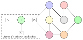
Figure 1: To implement privacy, at each time $k$ agent $j$ adds privacy noise $v_{j}(k)$ to its state $x_{j}(k)$ to obtain $\tilde{x}_{j}(k).$ Then at each time $k$, $\tilde{\bar{x}}_{j}(k)=\tilde{x}_{j}(k)-p_{j}$ is shared with agent $j$’s neighbors in $N_{j}$. Each agent uses this same setup to implement differential privacy for its own state trajectory.

When each agent implements privacy as illustrated above, agent $i$ only has access to $\tilde{x}_{j}(k)$ for $j\in N_{i}$. Plugging this into the node-level formation control protocol in (1) gives

$$\bar{x}_{i}(k+1)=\bar{x}_{i}(k)+\gamma\sum_{j\in N_{i}}w_{ij}(\tilde{\bar{x}}_{j}(k)-\bar{x}_{i}(k))+n_{i}(k).$$ (7)

This solves Problem 1.1.

To solve Problems 1.ii and 1.iii, we will analyze this protocol at the network level. For analysis, let $x_{[l]}=[x_{1_{[l]}},\dots,x_{N_{[l]}}]^{T}$, $p_{[l]}=[p_{1_{[l]}},\dots,p_{N_{[l]}}]^{T},$ and $\bar{x}_{[l]}=x_{[l]}-p_{[l]}$. Also let ${\Sigma_{v}=\textnormal{diag}(\sigma_{1}^{2},\dots,\sigma_{N}^{2})}$ and $\Sigma_{n}=\textnormal{diag}(s_{1}^{2},\dots,s_{N}^{2})$ We begin by formulating the network-level dynamics in each coordinate.

Lemma 2

Let a network of $N$ agents communicate over the weighted, simple graph $\mathcal{G}$ with Laplacian $L(\mathcal{G})$ and adjacency matrix $A(\mathcal{G})$. Suppose that agent $j$ uses privacy parameters $\epsilon_{j}>0$ and $\delta_{j}\in(0,1/2)$ and the adjacency parameter $b_{j}>0$. Suppose it uses the Gaussian mechanism to generate private states via $\tilde{x}_{j}(k)=x_{j}(k)+v_{j}(k)$, where $v_{j}(k)\sim\mathcal{N}(0,\sigma_{j}^{2}I_{d})$ and $\sigma_{j}\geq\kappa(\delta_{j},\epsilon_{j})b_{j}$ as in Lemma 1. Then when each agent implements the protocol in (7), the network-level dynamics are

$$\bar{x}_{[l]}(k+1)=(I_{N}-\gamma L(\mathcal{G}))\bar{x}_{[l]}(k)+z_{[l]}(k),$$

for each $l\in\{1,\dots,d\}$, where $z_{[l]}(k)\sim\mathcal{N}(0,\Sigma_{z}),$ ${\Sigma_{z}=\gamma^{2}A(\mathcal{G})\Sigma_{v}A(\mathcal{G})+\Sigma_{n}},\Sigma_{v}=\textnormal{diag}(\sigma_{1}^{2},\dots\sigma_{N}^{2})$ and $\Sigma_{n}=\textnormal{diag}(s_{1}^{2},\dots,s_{N}^{2})$.

Proof:

See Appendix -A. ∎

Then to analyze network-level performance, let $\beta_{[l]}(k):=\frac{1}{N}\mathbb{1}^{T}\bar{x}_{[l]}(k)\mathbb{1},$ which is the state vector the protocol in (6) would converge to with initial state $x_{[l]}(k)$ and without privacy or process noise. Also let

$$e_{[l]}(k)=\bar{x}_{[l]}(k)-\beta_{[l]}(k),$$ (8)

which is the offset of the current state from the state the protocol would converge to without noise. We analyze this error term in the next section.

IV Performance of Differentially Private Formation Control

In this section we solve Problem 1.ii. First, in Section IV-A we derive network-level error dynamics and show that the total mean square error, $e_{ss},$ can be computed using the trace of a solution to a Lyapunov equation. Then, we use these results in Section IV-B to derive several performance bounds that are functions of the underlying graph topology and each agent’s privacy parameters.

In this work we use the total mean square error of the network at steady-state, denoted $e_{ss}$, to quantify performance. Agent $i$’s private formation control protocol in (7) is in $\mathbb{R}^{d}$, and each agent in the network runs this protocol. This is equivalent to running $d$ identical copies of (6), which is in $\mathbb{R}^{N}$. Thus using (6), we can compute the mean square error in dimension $l$ and then multiply by $d$ to compute $e_{ss}$. The mean-square error in dimension $l$ is equal to $\lim_{k\to\infty}\frac{1}{N}\sum_{i=1}^{N}E[e^{2}_{[l],i}(k)],$ where $e_{[l],i}(k)$ is the $i^{th}$ element of $e_{[l]}(k).$ Then we have

$$e_{ss}:=\lim_{k\to\infty}\frac{d}{N}\sum_{i=1}^{N}E\left[e_{[l],i}^{2}(k)\right].$$

IV-A Connections with the Lyapunov Equation

The main error bound in this paper uses the fact that we can represent the total error in the system as the trace of a covariance matrix. We define $\Sigma_{e_{[l]}}(k)=E\left[e_{[l]}(k)e_{[l]}(k)^{T}\right]$ and $\Sigma_{\infty}=\lim_{k\to\infty}\Sigma_{e_{[l]}}(k).$ Then we have $e_{ss}=\frac{d}{N}Tr(\Sigma_{\infty}).$ Now we will analyze the dynamics of $e_{[l]}(k)$ and $\Sigma_{e_{[l]}}(k)$. For a given $\gamma>0$ and a given graph $\mathcal{G}$, let ${\mathcal{M}=I_{N}-\gamma L(\mathcal{G})-\frac{1}{N}\mathbb{1}\mathbb{1}^{T}}.$ Then we have the following.

Lemma 3

Let $N$ agents communicate over a given weighted, undirected, simple graph $\mathcal{G}$ with Laplacian $L(\mathcal{G})$ and adjacency matrix $A(\mathcal{G})$. Suppose for all $i$ that agent $i$ implements differential privacy using the Gaussian mechanism in Lemma 1 with privacy parameters $\epsilon_{i}>0$ and $\delta_{i}\in(0,\frac{1}{2}).$ When agent $i$ implements the private formation control protocol (7), the network level error $e_{[l]}(k)$ in (8) evolves via

$$e_{[l]}(k+1)=\mathcal{M}e_{[l]}(k)+(I_{N}-\frac{1}{N}\mathbb{1}\mathbb{1}^{T})z_{[l]}(k),$$ (9)

$\Sigma_{e_{[l]}}(k)$ evolves according to

$$\Sigma_{e_{[l]}}(k+1)=\mathcal{M}\Sigma_{e_{[l]}}(k)\mathcal{M}+(I_{N}-\frac{1}{N}\mathbb{1}\mathbb{1}^{T})\Sigma_{z}(I_{N}-\frac{1}{N}\mathbb{1}\mathbb{1}^{T}),$$ (10)

and $\Sigma_{e_{[l]}}(k)$ can be computed via

$$\Sigma_{e_{[l]}}(k)=\sum_{i=0}^{k-1}\mathcal{M}^{i}(I_{N}-\frac{1}{N}\mathbb{1}\mathbb{1}^{T})\Sigma_{z}(I_{N}-\frac{1}{N}\mathbb{1}\mathbb{1}^{T})\mathcal{M}^{i}.$$ (11)

Proof:

See Appendix -B. ∎

Lemma 4

Let $N$ agents communicate over a given weighted, undirected, simple, connected graph $\mathcal{G}$ with Laplacian $L(\mathcal{G})$ and ${\mathcal{M}=I_{N}-\gamma L(\mathcal{G})-\frac{1}{N}\mathbb{1}\mathbb{1}^{T}}.$ Then the eigenvalues of $\mathcal{M}$ are strictly less than $1.$ Furthermore, the maximum singular value of $\mathcal{M}$ is given by

$$\sigma_{\max}(\mathcal{M})=1-\gamma\lambda_{2}(L).$$ (12)

Proof:

See Appendix -C ∎

We now show that the steady-state error covariance matrix, $\Sigma_{\infty},$ is a solution to a discrete-time Lyapunov equation.

Theorem 1

Let $N$ agents communicate over a given undirected, simple graph $\mathcal{G}$ with weighted Laplacian $L(\mathcal{G})$ and adjacency matrix $A(\mathcal{G})$. Suppose that agent $i$ implements differential privacy using the Gaussian mechanism with privacy parameters $\epsilon_{i}>0$ and $\delta_{i}\in(0,\frac{1}{2})$ and implements the private formation control protocol (7). If the underlying graph $\mathcal{G}$ is connected, $\Sigma_{\infty}$ is equal to the unique solution to the discrete time Lyapunov equation

$$\Sigma_{\infty}=Q+\mathcal{M}\Sigma_{\infty}\mathcal{M},$$ (13)

where $Q=(I_{N}-\frac{1}{N}\mathbb{1}\mathbb{1}^{T})\Sigma_{z}(I_{N}-\frac{1}{N}\mathbb{1}\mathbb{1}^{T})$.

Proof:

From Lemma 3, we have

$$\Sigma_{\infty} =\lim_{k\to\infty}\Sigma_{e_{[l]}}(k)$$ (14)

$$=\sum_{i=0}^{\infty}\mathcal{M}^{i}(I_{N}-\frac{1}{N}\mathbb{1}\mathbb{1}^{T})\Sigma_{z}(I_{N}-\frac{1}{N}\mathbb{1}\mathbb{1}^{T})\mathcal{M}^{i}.$$ (15)

Taking the first term out of the sum gives

$$\Sigma_{\infty}=Q+\sum_{i=1}^{\infty}\mathcal{M}^{i}Q\mathcal{M}^{i}.$$ (16)

Factoring out $\mathcal{M}$ on both sides of the sum gives

$$\Sigma_{\infty}=Q+\mathcal{M}\left(\sum_{i=1}^{\infty}\mathcal{M}^{i-1}Q\mathcal{M}^{i-1}\right)\mathcal{M}.$$

The remaining infinite sum is precisely $\Sigma_{\infty}$. Thus, we arrive at the equation $\Sigma_{\infty}=Q+\mathcal{M}\Sigma_{\infty}\mathcal{M},$ which is the discrete-time Lyapunov equation. From Lemma 4, $\mathcal{M}$ has eigenvalues strictly less than $1$ for any undirected, connected graph $\mathcal{G}$ and $Q$ is positive definite. Using Proposition 2.1 from [30], (13) has a unique, symmetric solution $\Sigma_{\infty}.$ ∎

Theorem 1, along with the fact that $e_{ss}=\frac{d}{N}Tr(\Sigma_{\infty})$, allows us to solve for $e_{ss}$. That is, given a communication topology $\mathcal{G}$ and set of privacy parameters $\{(\epsilon_{i},\delta_{i})\}_{i=1}^{N},$ we can determine the performance of the network, encoded by $e_{ss},$ before runtime.

In this work, we are interested in designing a communication topology that allows agents to be as private as possible while meeting performance constraints. These performance constraints will take the form of $e_{ss}\leq e_{R}$ where $e_{R}$ is the maximum allowable error at steady-state. While Theorem 1 provides a means to evaluate the performance of a given network, it does not help us in designing a network to meet a specified performance requirement of the form $e_{ss}\leq e_{R}$. For example, if we are given a communication topology $\mathcal{G}$ and set of privacy parameters $\{(\epsilon_{i},\delta_{i})\}_{i=1}^{N},$ we can use Theorem 1 to compute $e_{ss}$ and can check if $e_{ss}\leq e_{R},$ but Theorem 1 does not provide a direct way to design a network that achieves $e_{ss}\leq e_{R}$ if the bound is not already met. In the next subsection, we find a scalar bound on $e_{ss}$ that will be used to solve network design problems of this type in Section V.

IV-B Analytical Result and Bounds

In this section we find a scalar bound on $e_{ss}$ in terms of the privacy parameters $\{(\epsilon_{i},\delta_{i})\}_{i=1}^{N},$ and properties of the communication toplogy $\mathcal{G}$ that will allow us to design networks that achieve given performance constraints. In the following theorem, the main bound is a result of $\Sigma_{\infty}$ being the solution to a Lyapunov equation as shown in Theorem 1. Several bounds and properties of Lyapunov equations have been explored in the literature, and some of these results have been surveyed in [31]. We have the following bound on $e_{ss}.$

Theorem 2

Let all the conditions from Theorem 1 hold. With

$$e_{ss}:=\lim_{k\to\infty}\frac{d}{N}\sum_{i=1}^{N}E\left[e_{[l],i}^{2}(k)\right],$$

we have

$$e_{ss}\leq\frac{\gamma d\sum_{i=1}^{N}\left(\sum_{j=1}^{N}w_{ij}^{2}-\frac{d_{i}^{2}}{N}\right)\sigma_{i}^{2}+\frac{N-1}{N}\sum_{i=1}^{N}s_{i}^{2}}{N\lambda_{2}(L)\left(2-\gamma\lambda_{2}(L)\right)}.$$

Proof:

See Appendix -D. ∎

Theorem 2 solves Problem 1.ii. This result gives a scalar bound on $e_{ss}$ that depends on the the privacy parameters $\{(\epsilon_{i},\delta_{i})\}_{i=1}^{N}$ through $\sigma_{i},$ where $\sigma_{i}\geq\kappa(\delta_{i},\epsilon_{i})b_{i}$, the edge weights in the graph $w_{ij},$ the weighted degree of each agent, the algebraic connectivity $\lambda_{2}(L),$ and the variance of the process noise $s_{i}^{2}.$

In the previous subsection we detailed how Theorem 1 was not sufficient for designing networks to meet performance constraints of the form $e_{ss}\leq e_{R}.$ Theorem 2 provides a method to enforce these constraints. For example, if the network must achieve $e_{ss}\leq e_{R}$ this can be achieved by requiring that

$$\frac{\gamma d\sum_{i=1}^{N}\left(\sum_{j=1}^{N}w_{ij}^{2}-\frac{d_{i}^{2}}{N}\right)\sigma_{i}^{2}+\frac{N-1}{N}\sum_{i=1}^{N}s_{i}^{2}}{N\lambda_{2}(L)\left(2-\gamma\lambda_{2}(L)\right)}\leq e_{R}.$$ (17)

This requirement will impose constraints on the communication topology $\mathcal{G},$ the weights in the communication topology $w_{ij},$ and privacy parameters $\{(\epsilon_{i},\delta_{i})\}_{i=1}^{N}.$ Overall, the bound on $e_{ss}$ in Theorem 2 gives us a method to translate a performance requirement into a joint constraint on the communication topology and privacy parameters. In the next section, we use this constraint to formulate an optimization problem where the privacy parameters and communication topology are the decision variables to design a private formation control network that allows agents to be as private as possible while meeting global performance requirements.

V Privacy and Network Co-design

In this section we solve Problem 1.iii. Given the aforementioned bounds on formation error, we now focus on designing networks for performing private formation control. Our goal is to design a network, through selecting entries of $L(\mathcal{G})$, and privacy scheme, through selecting the values of $\{\epsilon_{i}\}_{i=1}^{N}$, that meet global performance requirements, agent-level privacy requirements, and other constraints. Here we keep $\delta_{i}$ fixed and tune $\epsilon_{i}$ to achieve the desired level of privacy. Since $\delta_{i}$ is the probability that differential privacy fails, the existing privacy literature is primarily focused on tuning $\epsilon_{i}$ and we do so here.

The key tradeoff in designing a private formation control network is balancing agent-level privacy requirements with global performance. For example, if some agents use very strong privacy, then the high-variance privacy noise they use will make global performance poor, even if many other agents have only weak privacy requirements. These effects can also be amplified or attenuated by the communication topology of the network, e.g., if an agent with strong privacy sends very noisy messages to other agents along heavily weighted edges. Privacy/network co-design thus requires unifying and balancing these tradeoffs while designing a weighted, undirected graph and the privacy levels that agents use.

V-A Co-Design Search Space

In this section we consider the following setup. We are given $N$ agents that wish to implement private formation control and each agent has a minimum strength of privacy that it will accept. We are tasked with designing a network that allows agents to be as private as possible while meeting a global performance requirement. In many settings, each agent’s neighborhood set will be fixed a priori based on hardware compatibility or physical location, and these neighborhoods specify an unweighted, undirected graph of edges that can be used.

As network designers, we must design the privacy parameters for each agent and all edge weights for the given graph. That is, we can assign a zero or non-zero weight to each edge that is present, but we cannot attempt to assign non-zero weight to an edge that is absent. We denote the given unweighted graph by $\mathcal{G}_{0}$ and denote its unweighted Laplacian by $L_{0}$. We define $\mathcal{L}(L_{0})$ as the space of all weighted graph Laplacians $L$ such that $L_{ij}=0$ if $L_{0,ij}=0$.

Thus, if the original undirected graph has $|E|$ edges, we must select $|E|+N$ parameters, namely one weight for each edge and the values of $\{\epsilon_{i}\}_{i=1}^{N}$. Designing these parameters manually for large networks will be infeasible and thus we develop a numerical framework for their design.

V-B Co-Design Problem Statement

Below we formally state the privacy/network co-design problem and then describe its features.

Problem 2 (Co-design Problem)

Given an input undirected, unweighted, simple graph $\mathcal{G}_{0}$ with Laplacian $L_{0},$ a required global error bound $e_{R},$ a minimum connectivity parameter $\lambda_{2_{L}},$ weighting factor $\vartheta,$ and a minimum level of privacy $\epsilon_{i}^{max}$ for agent $i$ for all $i\in[N]$, to co-design privacy and agents’ communication topology, solve

$$\min_{L(\mathcal{G})\in\mathcal{L}(L_{0}),\{\epsilon_{i}\}_{i=1}^{N}}\quad\textnormal{Tr}(L(\mathcal{G}))+\vartheta\sum_{i=1}^{N}\epsilon_{i}^{2}$$ (18)

subject to $$\frac{\gamma d\sum_{i=1}^{N}\!\left(\sum_{j=1}^{N}\!w_{ij}^{2}\!-\!\frac{d_{i}^{2}}{N}\right)\sigma_{i}^{2}\!+\!\frac{N-1}{N}\!\sum_{i=1}^{N}\!s_{i}^{2}}{\lambda_{2}(L)\left(2-\gamma\lambda_{2}(L)\right)}\!\leq\!e_{R}$$ (19)

$$\quad\epsilon_{i}\leq\epsilon_{i}^{max}\quad\textnormal{for all }i$$ (20)

$$\lambda_{2}(L(\mathcal{G}))\geq\lambda_{2_{L}}.$$ (21)

$\triangle$

First, we describe the objective function of Problem 2. In the objective function, the purpose of $Tr(L(\mathcal{G}))$ is to produce a network that uses as little edge weight as possible. In Theorem 2, the numerator of the error bound grows as $w_{ij}$ grows. With $Tr(L(\mathcal{G}))=\sum_{i\in[N]}d_{i},$ minimizing this will produce a solution where each agent has a small degree, which promotes better network-level performance. If edge weights represent or are correlated to a monetary cost, minimizing $Tr(L(\mathcal{G}))$ also produces a solution that will use as little cost as possible. For the other term in the objective function, $\sum_{i\in[N]}\epsilon_{i}^{2},$ minimizing this function will make each agent’s privacy level as strong as possible; since the strength of privacy grows as $\epsilon_{i}$ shrinks, this term will force the solution to have a strong level of privacy for each agent. The weighting factor $\vartheta\in\mathbb{R}$ allows the user to prioritize a solution with a strong level of privacy or small degrees for each agent.

We now describe the constraints of Problem 2. The first constraint requires that the total mean square error of the network, $e_{ss},$ is less than some user-defined value $e_{R}$. A sufficient condition for $e_{ss}\leq e_{R}$ can be found by requiring that the bound in Theorem 2 is less than $e_{R},$ which is what we implement here. The second constraint requires that each agent’s privacy level is at least as strong as that agent’s weakest acceptable privacy level, which is set by $\epsilon_{i}^{max}$. The last constraint requires that the solution produces a connected graph. Connectivity for the weighted graph can be ensured by $\lambda_{2}(L(\mathcal{G}))>0$, but we implement the constraint $\lambda_{2}(L(\mathcal{G}))\geq\lambda_{2_{L}}$ for some user defined $\lambda_{2_{L}}>0$ so the user has some control over how connected the resulting graph is. For example, $\lambda_{2_{L}}$ can be set to the algebraic connectivity of the line graph on $N$ nodes, which has the least algebraic connectivity among graphs on $N$ nodes.

Overall, solving Problem 2 will produce a communication topology and privacy parameters that will meet global performance and connectivity constraints while allowing agents to be as private as possible. This solves Problem 1.iii.

V-C Numerically Solving Problem 2

We have built a MATLAB program to solve Problem 2, which is available on GitHub [32]. Due to the non-linearities in the problem, i.e., some of our constraints are in terms of the second largest eigenvalue of one of our decision variables, we found MATLAB and fmincon to perform well for problems of this kind. When optimizing over $L(\mathcal{G})\in\mathcal{L}(L_{0}),$ since we only consider undirected, symmetrically weighted graphs, we need only find the upper triangular elements of $L(\mathcal{G})$, which helps reduce computation time. Further commentary and examples are provided in the next section.

VI Simulations

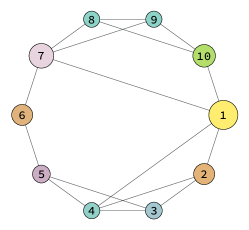
Figure 2: The fixed input topology used for the simulation results presented in Section VI. This topology contains $10$ nodes and specifies the edges that can be present, though the edge weights are not specified and will be optimized over.

In this section we provide simulation results for optimal privacy/network co-design. There are four main parameters that we have control over in Problem 2: (i) $e_{R},$ to control the performance of the system, (ii) $\epsilon^{max}_{i},$ to specify the weakest allowable privacy level for agent $i$, (iii) $\lambda_{2L},$ to control the connectivity of the designed network, and (iv) $\vartheta,$ which weights optimizing performance versus privacy. In this section, we first define an input topology as the undirected, simple graph $\mathcal{G}$ shown in Figure 2. Then, we manually tune the parameters $e_{R},\epsilon_{i}^{max},\lambda_{2_{L}},$ and $\vartheta,$ and run privacy/network co-design for various sets of parameters to obtain a weighted graph and set of privacy parameters $\{\epsilon_{i}\}_{i=1}^{N}$.

Throughout this section the smaller a node is drawn the more private it is, i.e., $\epsilon_{i}$ gets smaller as node $i$ shrinks, and the thicker an edge is drawn the more weight it has. In simulation, edges with weights satisfying $w_{ij}<10^{-4}$ are considered deleted. We begin by manually adjusting $e_{R}$ with all other parameters fixed.

Example 1: (Trading off privacy and performance) Fix the input graph $\mathcal{G}$ shown in Figure 2. Fix

$$\epsilon^{max}=[0.4,0.9,0.55,0.35,0.8,0.45,0.7,0.5,0.52,0.58]^{T},$$

$\gamma=1/2N,\vartheta=10,$ $\lambda_{2L}=0.2,$ $\delta_{i}=0.05,$ and $b_{i}=1$ for all $i.$ Now let $e_{R}$ take on the values

$$e_{R}\in\{2,4,8,16,32,64\}.$$

For each of these values, privacy/network co-design was used to design the weighted graphs shown in Figure 4 and the privacy parameters shown in Figure 5.

In Figure 4, as we allow weaker performance, quantified by larger $e_{R},$ the agents are able to use a stronger level of privacy. This is illustrated by the nodes shrinking as $e_{R}$ increases from Figure LABEL:fig:biggest_er to LABEL:fig:smallest_er. Furthermore, privacy/network co-design makes the resulting graph less connected when we allow weaker performance. For example, when comparing Figure LABEL:fig:biggest_er to Figure LABEL:fig:smallest_er, the output network topology has fewer edges when weaker performance is allowed.

In Figure 5, we can see that as the required level of performance decreases, co-design allows the agents to be more private. This trend persists for all agents in varying magnitude which is influenced by the topology and each $\epsilon_{i}^{max}.$ We can also see that $\epsilon_{i}$ decreases rapidly from $e_{R}=2$ to $e_{R}=8,$ and then decreases slower for $e_{R}>8.$ This shows that relatively small changes in $e_{R}$ can lead to large changes in the resulting privacy level, i.e., if we relax performance slightly it is possible to gain a much stronger level of privacy, which occurs when $\epsilon_{i}$ is small for each agent. $\triangle$

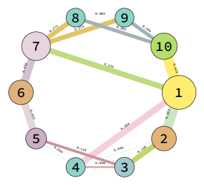
(a)

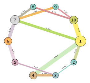
(b)

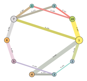
(c)

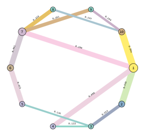
(d)

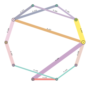
(e)

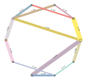
(f)

Figure 4: The outputs of privacy/network co-design with fixed parameters specified in Example $1$ for different values of $e_{R}\in\{2,4,8,16,32,64\}.$ The smaller a node is drawn, the more private it is, i.e., its value of $\epsilon_{i}$ is smaller. The thicker an edge is drawn, the larger the edge weight, i.e., $w_{ij}$ is larger. We can see that when we allow weaker performance, indicated by larger $e_{R},$ each agent has a stronger level of privacy and the topology uses less weight as illustrated by the nodes shrinking from Figure LABEL:fig:biggest_er to Figure LABEL:fig:smallest_er. Furthermore, privacy/network co-design makes the resulting graph less connected when we allow weaker performance. For example, when comparing Figure LABEL:fig:biggest_er to Figure LABEL:fig:smallest_er, the output network topology has fewer edges when weaker performance is allowed.

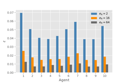
Figure 5: The numerical values of privacy parameters as designed by privacy/network co-design with fixed parameters specified in Example $1$ and $e_{R}\in\{2,16,64\}.$ As the required level of performance decreases, co-design allows the agents to be more private. This trend persists for all agents.

Example 2: (The Maximum Level of Privacy) Here we fix all of the parameters other than $\epsilon_{i}^{max}.$ Specifically, fix ${\gamma=1/2N},\lambda_{2L}=0.2,$ $\vartheta=10,e_{R}=2,\delta_{i}=0.05,$ and $b_{i}=1$ for all $i.$ We consider the homogeneous case where each agent has the same required level of privacy, i.e., $\epsilon_{i}^{max}=\epsilon^{max}$ for $i\in\{1,\dots,N\}.$ Privacy/network co-design was run for $\epsilon^{max}\in\{0.03,0.04,0.05\}.$ Figure 6 presents the output communication topologies and Figure 7 shows the output privacy parameters for each agent as designed by privacy/network co-design.

In Figure 6, we can see that as we allow each agent to be less private, co-design actually removes edges. Specifically the edges $(8,9),(2,4),$ and $(4,5)$ in Figure 6(a) when $\epsilon^{max}=0.03$ are not present in Figure 6(c) when $\epsilon^{max}=0.05.$ This shows that co-design is trying to use as little edge weight or as few edges as possible to meet the constraints. In others words, when each agent uses less privacy, i.e., larger $\epsilon_{i}$ and $\epsilon^{max}$ for each agent $i,$ co-design designs a network with less communication to achieve the same level of performance.

In Figure 7, we can see that when $\epsilon_{i}^{max}=0.03,$ each $\epsilon_{i}$ is close to $\epsilon_{i}^{max},$ i.e., the agents are using the weakest privacy possible. This occurs because, with $e_{R}=2,$ we require relatively strong performance, which limits the strength of agents’ privacy. As a result, when $\epsilon_{i}^{max}=0.03$ privacy/network co-design finds the optimal network to be one in which each agent uses the weakest privacy possible, i.e., $\epsilon_{i}$ is small and significantly less than $\epsilon_{i}^{max}$ for each $i.$ This is because with a stronger level of privacy, the communication topology needs to be more connected, which causes $\textnormal{Tr}(L(\mathcal{G}))$ in the objective function of Problem 2 to grow. However, when $\epsilon_{i}^{max}\in\{0.04,0.05\}$ the agents are using stronger privacy than the weakest level they specified, as the resulting $\epsilon_{i}$’s are not at their constrained maximum. $\triangle$

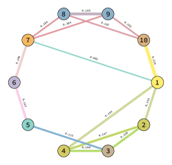
(a)

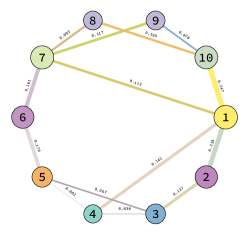
(b)

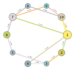
(c)

Figure 6: The outputs of privacy/network co-design with fixed parameters specified in Example $2$ for different values of $\epsilon_{i}^{max}\in\{0.03,0.04,0.05\}.$ The smaller a node is drawn, the more private it is, i.e., its value of $\epsilon_{i}$ is smaller. The thicker an edge is drawn, the larger the edge weight, i.e., $w_{ij}$ is larger. As we allow each agent to be less private, the network actually removes edges. Specifically, the edges $(8,9),(2,4),$ and $(4,5)$ in Figure 6(a) are not present in Figure 6(c). This shows that co-design is trying to use as little edge weight or as few edges as possible to meet the constraints, and when agents are less private they need less communication to achieve the same level of performance.

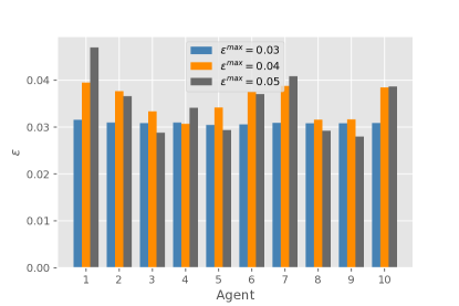
Figure 7: The numerical values of privacy parameters as designed by privacy/network co-design with fixed parameters specified in Example $2$ and $\epsilon_{i}^{max}\in\{0.03,0.04,0.05\}.$ When $\epsilon_{i}^{max}=0.03,$ the agents are using the weakest privacy possible, which occurs because $e_{R}=2$ requires relatively strong performance, and agents must share more information to facilitate this. However, when $\epsilon_{i}^{max}\in\{0.04,0.05\}$ the agents are using stronger privacy than the weakest level they specified, as the resulting $\epsilon_{i}$’s are not at their constrained maximum.

Example 3: (The Minimum Level of Connectivity) Here we fix all of the parameters other than $\lambda_{2L}.$ Specifically, fix $\gamma=1/2N,\lambda_{2L}=0.2,$ $\vartheta=10,$ $e_{R}=1,$ $\delta_{i}=0.05,b_{i}=1$ for all $i,$ and

$$\epsilon^{max}=[0.4,0.9,0.55,0.35,0.8,0.45,0.7,0.5,0.52,0.58]^{T}.$$

Then we solve the privacy/network co-design problem for $\lambda_{2L}\in\{0.1,0.5,1\}.$ Figure 8 gives the output communication topologies and Figure 9 shows the output privacy parameters for each agent.

In Figure 8, we can see that as we require the output network to be more connected, more edge weight is used and each agent uses weaker privacy, as illustrated by the growing nodes and edges from Figure LABEL:fig:smallest_lambda to Figure LABEL:fig:biggest_lambda. We can also see that co-design is adding weight to certain edges more than others. Specifically, the weight of the edge $(1,7)$ drastically increases while the weight of the edge $(9,10)$ does not increase much. Agents $9$ and $10$ are more private than agents $1$ and $7$ when $\lambda_{2L}=1.0$ as illustrated by the size of the nodes in Figure 8. Thus, privacy/network co-design is using smaller edge weights for agents with stronger privacy. This makes intuitive sense since agents with strong privacy inject higher-variance noise into the formation control protocol then agents with weaker privacy, and reducing the weights of edges connected to those agents with weaker noise helps mitigate this impact.

In Figure 9, as $\lambda_{2L}$ is increased, $\epsilon_{i}$ increases for most agents, i.e., as the network is required to be more connected, the agents use weaker privacy. Here privacy/network co-design adds the necessary edge weight to meet the connectivity constraint, and then weakens privacy to meet the performance constraint. Thus privacy/network co-design is trading off privacy and performance as desired. $\triangle$

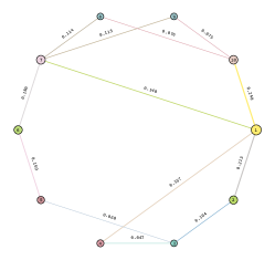
(a)

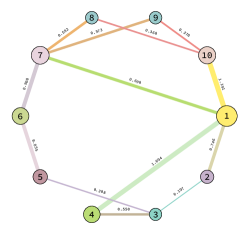
(b)

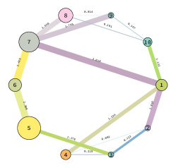
(c)

Figure 8: The outputs of privacy/network co-design with fixed parameters specified in Example $3$ for different values of $\lambda_{2L}\in\{0.1,0.5,1\}.$ The smaller a node is drawn, the more private it is, i.e., its value of $\epsilon_{i}$ is smaller. The thicker an edge is drawn, the larger the edge weight, i.e., $w_{ij}$ is larger. As we require the output network to be more connected, more edge weight is used and each agent uses weaker privacy. When $\lambda_{2L}=1,$ the output $\epsilon_{i}$ is close to $\epsilon_{i}^{max}$ for each $i.$ Here privacy/network co-design is adding edge weight to meet the connectivity constraint, and then weakens privacy to meet the performance constraint, thus trading off privacy and performance as desired.

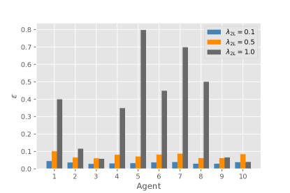
Figure 9: The numerical values of privacy parameters as designed by privacy/network co-design with fixed parameters specified in Example $3$ and $\lambda_{2L}\in\{0.1,0.5,1\}.$ As the output is required to be more connected, increasing $\lambda_{2L},$ each agent uses weaker privacy. When $\lambda_{2L}=1,$ the largest value, the agents are using near their weakest required level of privacy in order to meet the performance requirement.

Example 4: (Tuning the Objective Function) Here we fix all parameters other than $\vartheta.$ Specifically, fix $\gamma=1/2N,\lambda_{2L}=0.2,$ $\lambda_{2L}=0.05,$ $e_{R}=1,\delta_{i}=0.05,$ and $b_{i}=1$ for all $i,$ and

$$\epsilon^{max}=[0.4,0.9,0.55,0.35,0.8,0.45,0.7,0.5,0.52,0.58]^{T}.$$

Then we solve the co-design problem for $\vartheta\in\{1,100,1000\}.$ Figure 10 presents the output communication topologies and Figure 11 shows the output privacy parameters for each agent.

In Figure 10, we can see that as we increase $\vartheta$ from $\vartheta=1$ in Figure LABEL:fig:smallest_var to $\vartheta=1000$ in Figure LABEL:fig:biggest_var each of the edge weights increase slightly. Intuitively, as we increase $\vartheta,$ we are prioritizing minimizing $\sum_{i=1}^{N}\epsilon_{i}^{2}$ rather than $\textnormal{Tr}(L(\mathcal{G})).$ As $\vartheta$ changes, the weights do not change very much, though the privacy levels change drastically as illustrated in Figure 11.

In Figure 11, we can see that as $\vartheta$ is increased, the output privacy parameters are much lower for each agent. When $\vartheta=1,$ the privacy parameters $\epsilon_{i}$ are near their constrained maxima, $\epsilon_{i}^{max}.$ When $\vartheta=1000,$ we are prioritizing minimizing $\sum_{i}\epsilon_{i}^{2}$ rather than $\textnormal{Tr}(L(\mathcal{G})),$ and thus the output privacy parameters are much smaller. Overall, this shows that increasing $\vartheta$ can be used to allow the agents to achieve a stronger level of privacy. $\triangle$

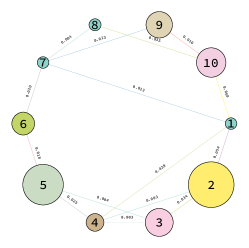
(a)

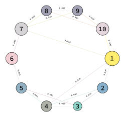
(b)

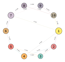
(c)

Figure 10: The outputs of privacy/network co-design with fixed parameters specified in Example $4$ for different values of $\vartheta\in\{1,100,1000\}.$ The smaller a node is drawn, the more private it is, i.e., its value of $\epsilon_{i}$ is smaller. The thicker an edge is drawn, the larger the edge weight, i.e., $w_{ij}$ is larger. As we increase $\vartheta,$ the edge weights increase. This is intuitive because as we increase $\vartheta$ we are prioritizing minimizing $\sum_{i}\epsilon_{i}^{2}$ rather than $\textnormal{Tr}(L(\mathcal{G})).$ Each agent also uses much stronger privacy as $\vartheta$ is increased, as illustrated by the size of each node shrinking from Figure LABEL:fig:smallest_var to Figure LABEL:fig:biggest_var and further illustrated in Figure 11.

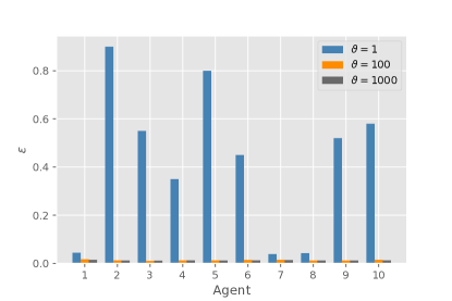
Figure 11: The numerical values of privacy parameters as designed by privacy/network co-design with fixed parameters specified in Example $4$ and $\vartheta\in\{1,100,1000\}.$ As $\vartheta$ is increased, the output privacy parameters are much lower for each agent. When $\vartheta=1,$ the privacy parameters $\epsilon_{i}$ are near their constrained maxima, $\epsilon_{i}^{max}.$ When $\vartheta=1000,$ we prioritize minimizing $\sum_{i}\epsilon_{i}^{2}$ rather than $\textnormal{Tr}(L(\mathcal{G})),$ and thus the output privacy parameters are much smaller. This further illustrates the flexibility of privacy/network co-design.

VII Conclusions

In this paper we have studied the problem of differentially private formation control. This work enables agents to collaboratively assemble into formations with bounded steady state error and provides methods for solving for the error covariance matrix at steady-state. This work also develops and solves an optimization problem to design the optimal network and privacy parameters for differentially private formation control. Future work includes generalizing to other privacy/performance co-design problems and implementation on mobile robots.

-A Proof of Lemma 2

From (7) we have the node level protocol

$$\bar{x}_{i}(k+1)=\bar{x}_{i}(k)+\gamma\sum_{j\in N_{i}}w_{ij}(\bar{x}_{j}(k)+v_{j}(k)-\bar{x}_{i}(k))+n_{i}(k),$$

which we factor as

$$\bar{x}_{i}(k+1)=\bar{x}_{i}(k)+\gamma\sum_{j\in N_{i}}w_{ij}(\bar{x}_{j}(k)-\bar{x}_{i}(k))$$

$$+\gamma\sum_{j\in N_{i}}w_{ij}v_{j}(k)+n_{i}(k).$$

Let $z_{i}(k)=\gamma\sum_{j\in N_{i}}w_{ij}v_{j}(k)+n_{i}(k)$ and note that

$$z_{i}(k)=\gamma\big{(}[A(\mathcal{G})]_{row\ i}\otimes I_{d}\big{)}v(k)+n_{i}(k),$$

where $[A(\mathcal{G})]_{row\ i}\in\mathbb{R}^{1\times n}$ is the $i^{th}$ row of $A(\mathcal{G})$ and $\otimes$ is the Kronecker product. Next we define the vector $z_{[l]}(k)=[z_{1_{[l]}}(k)^{T},\dots,z_{N_{[l]}}(k)^{T}]^{T}\in\mathbb{R}^{N}$ and we have $z_{[l]}(k)=\gamma A(\mathcal{G})v_{[l]}(k)+n_{[l]}(k)$ at the network level. Since $v_{[l]}(k)$ and $n_{[l]}(k)$ are zero mean, $z_{[l]}(k)$ is zero mean. The covariance of $z_{[l]}(k)$ is calculated as

$$\Sigma_{z} =E[z_{[l]}(k)z_{[l]}(k)^{T}]$$ (22)

$$=E[\left(\gamma A(\mathcal{G})v_{[l]}(k)+n_{[l]}(k)\right)\left(\gamma A(\mathcal{G})v_{[l]}(k)+n_{[l]}(k)\right)^{T}].$$ (23)

Then, since $v_{[l]}(k)$ and $n_{[l]}(k)$ are statistically independent, $E[v_{[l]}(k)n_{[l]}(k)^{T}]=E[n_{[l]}(k)v_{[l]}(k)^{T}]=0$. Applying this fact, the linearity of expectation, and the symmetry of $A(\mathcal{G})$ gives

$$\Sigma_{z} =\gamma^{2}A(\mathcal{G})E[v_{[l]}(k)v_{[l]}(k)^{T}]A(\mathcal{G})+E[n_{[l]}(k)n_{[l]}(k)^{T}]$$ (24)

$$=\gamma^{2}A(\mathcal{G})\Sigma_{v}A(\mathcal{G})+\Sigma_{n}.$$ (25)

Then $z_{[l]}(k)\sim\mathcal{N}(0,\gamma^{2}A(\mathcal{G})\Sigma_{v}A(\mathcal{G})+\Sigma_{n})).$ $\blacksquare$

-B Proof of Lemma 3

First, we expand $e_{[l]}(k+1),$

$$e_{[l]}(k+1) =\bar{x}_{[l]}(k+1)-\beta_{[l]}(k+1)$$

$$=\bar{x}_{[l]}(k+1)-\frac{1}{N}\mathbb{1}^{T}\bar{x}_{[l]}(k+1)\mathbb{1}$$

$$=\left(I_{N}-\frac{1}{N}\mathbb{1}\mathbb{1}^{T}\right)x_{[l]}(k+1)$$

$$=\left(I_{N}-\frac{1}{N}\mathbb{1}\mathbb{1}^{T}\right)\left((I_{N}-\gamma L(\mathcal{G}))\bar{x}_{[l]}(k)+z_{[l]}(k)\right).$$

Expanding further gives

$$e_{[l]}(k+1) =\left(I_{N}-\gamma L(\mathcal{G})-\frac{1}{N}\mathbb{1}\mathbb{1}^{T}\right)\bar{x}_{[l]}(k)$$ (26)

$$+\left(I_{N}-\frac{1}{N}\mathbb{1}\mathbb{1}^{T}\right)z_{[l]}(k),$$ (27)

where we have used the fact that $L(\mathcal{G})\mathbb{1}=0.$ Let ${\mathcal{M}=I_{N}-\gamma L(\mathcal{G})-\frac{1}{N}\mathbb{1}\mathbb{1}^{T}}$ and note that

$$\mathcal{M}\beta_{[l]}(k)=\left(I_{N}-\frac{1}{N}\mathbb{1}\mathbb{1}^{T}\right)\beta_{[l]}(k)=0.$$

Then we have

$$e_{[l]}(k+1) =\mathcal{M}\bar{x}_{[l]}(k)+\left(I_{N}-\frac{1}{N}\mathbb{1}\mathbb{1}^{T}\right)z_{[l]}(k)$$

$$=\mathcal{M}\left(\bar{x}_{[l]}(k)-\beta_{[l]}(k)\right)+\left(I_{N}-\frac{1}{N}\mathbb{1}\mathbb{1}^{T}\right)z_{[l]}(k)$$

$$=\mathcal{M}e_{[l]}(k)+\left(I_{N}-\frac{1}{N}\mathbb{1}\mathbb{1}^{T}\right)z_{[l]}(k),$$

which proves (9). Plugging this into the definition of $\Sigma_{e_{[l]}}(k+1)$ gives

$$\Sigma_{e_{[l]}}(k+1) =E\left[e(k+1)e(k+1)^{T}\right]$$

$$=\mathcal{M}E\left[e_{[l]}(k)e_{[l]}(k)^{T}\right]\mathcal{M}$$

$$+\left(I_{N}-\frac{1}{N}\mathbb{1}\mathbb{1}^{T}\right)\Sigma_{z}\left(I_{N}-\frac{1}{N}\mathbb{1}\mathbb{1}^{T}\right)$$

$$=\mathcal{M}\Sigma_{e_{[l]}}(k)\mathcal{M}+\left(I_{N}-\frac{1}{N}\mathbb{1}\mathbb{1}^{T}\right)\Sigma_{z}\left(I_{N}-\frac{1}{N}\mathbb{1}\mathbb{1}^{T}\right),$$

which proves (10). Then (11) follows by applying (10) recursively. $\blacksquare$

-C Proof of Lemma 4

We begin by analyzing the eigenvalues of $\mathcal{M}.$ Note that $\mathcal{M}\mathbb{1}=0,$ and thus $\mathcal{M}$ has eigenvalue $0$ with eigenvector $\mathbb{1}.$ Now let $(\lambda,\ v)$ be an eigenpair of $\mathcal{M}$ with $\lambda\neq 0.$ We now show that $\lambda\neq 0$ implies that $(\lambda,\ v)$ is also an eigenpair of $I-\gamma L(\mathcal{G}).$ Since $\mathcal{G}$ is connected and undirected, $I-\gamma L(\mathcal{G})$ is a doubly stochastic matrix, it has one eigenvalue of modulus $1$ which is $\lambda(I-\gamma L(\mathcal{G}))=1$ with an eigenvector of $\mathbb{1}$, and the rest of the eigenvalues are positive and lie strictly in the unit disk [26, Lemma 3].

Using $\mathbb{1}^{T}(I_{N}-\gamma L(\mathcal{G}))=\mathbb{1}^{T},$ we have

$$\mathbb{1}^{T}v=\mathbb{1}^{T}(I_{N}-\gamma L(\mathcal{G}))v.$$

Adding and subtracting $\mathbb{1}^{T}(\frac{1}{N}\mathbb{1}\mathbb{1}^{T})v$ gives

$$\mathbb{1}^{T}v =\mathbb{1}^{T}(I_{N}-\gamma L(\mathcal{G}))v-\mathbb{1}^{T}(\frac{1}{N}\mathbb{1}\mathbb{1}^{T})v+\mathbb{1}^{T}(\frac{1}{N}\mathbb{1}\mathbb{1}^{T})v$$

$$=\mathbb{1}^{T}\mathcal{M}v+\mathbb{1}^{T}(\frac{1}{N}\mathbb{1}\mathbb{1}^{T})v,$$

then plugging in $\mathcal{M}v=\lambda v$ and $\mathbb{1}^{T}(\frac{1}{N}\mathbb{1}\mathbb{1}^{T})=\mathbb{1}^{T}$ gives

$$\mathbb{1}^{T}v =\lambda\mathbb{1}^{T}v+\mathbb{1}^{T}v$$

$$=(\lambda+1)\mathbb{1}^{T}v.$$

Since $\lambda\neq 0,$ we must have $\mathbb{1}^{T}v=0$ for the above to be true. This implies that $v$ is orthogonal to $\mathbb{1}.$ Furthermore we have that $(\frac{1}{N}\mathbb{1}\mathbb{1}^{T})v=0,$ so

$$\lambda v =\mathcal{M}v=(I_{N}-\gamma L(\mathcal{G})-\frac{1}{N}\mathbb{1}\mathbb{1}^{T})v$$

$$=(I_{N}-\gamma L(\mathcal{G}))v.$$

This means that any non-zero eigenvalue of $\mathcal{M}$ is also an eigenvalue of $I-\gamma L(\mathcal{G})$ and the associated eigenvector $v$ is orthogonal to $\mathbb{1}.$

Furthermore, $L(\mathcal{G})$ and $I_{N}-\gamma L(\mathcal{G})$ have the same eigenvectors and we have that

$$\lambda_{i}(I_{N}-\gamma L(\mathcal{G}))=1-\gamma\lambda_{i}(L(\mathcal{G})).$$

Thus, $\lambda_{i}(\mathcal{M})=1-\gamma\lambda_{i}(L(\mathcal{G}))$ for ${i\in\{2,\dots,N\}}.$ With the sorting $\lambda_{2}(L(\mathcal{G}))\leq\dots\leq\lambda_{N}(L(\mathcal{G})),$ we have that $\lambda_{\max}(\mathcal{M})=1-\gamma\lambda_{2}(L(\mathcal{G}))<1.$ This implies that all eigenvalues of $\mathcal{M}$ lie strictly in the unit disk.

Now $\sigma_{\max}(\mathcal{M})=(1-\gamma\lambda_{2}(L))$ follows from the fact that

$$\left[\sigma_{\max}(\mathcal{M})\right]^{2} =\left[\left(\lambda_{\max}\left((\mathcal{M})(\mathcal{M})\right)\right)^{1/2}\right]^{2}$$ (28)

$$=\lambda_{\max}\left((\mathcal{M})^{2}\right)$$ (29)

$$=\lambda_{\max}\left((\mathcal{M})\right)^{2}$$ (30)

$$=\left(1-\gamma\lambda_{2}(L(\mathcal{G}))\right)^{2}.$$ (31)

$\blacksquare$

-D Proof of Theorem 2

First, with Theorem 1 and [31, Equation 151] [33] we can bound $Tr\left(\Sigma_{\infty}\right)$ as

$$Tr\left(\Sigma_{\infty}\right)\leq\frac{Tr(Q)}{1-\left(\sigma_{\max}(\mathcal{M})\right)^{2}},$$ (32)

where $\sigma_{\max}(\mathcal{M})$ denotes the maximum singular value of $\mathcal{M}.$

We start by expanding $Tr(Q)$ in (32), which gives

$$Tr(Q) =Tr\left((I_{N}-\frac{1}{N}\mathbb{1}\mathbb{1}^{T})\Sigma_{z}(I_{N}-\frac{1}{N}\mathbb{1}\mathbb{1}^{T})\right).$$

Applying cyclic permutation of the trace gives

$$Tr(Q) =Tr\left((I_{N}-\frac{1}{N}\mathbb{1}\mathbb{1}^{T})(I_{N}-\frac{1}{N}\mathbb{1}\mathbb{1}^{T})\Sigma_{z}\right).$$ (33)

Note that $(I_{N}-\frac{1}{N}\mathbb{1}\mathbb{1}^{T})(I_{N}-\frac{1}{N}\mathbb{1}\mathbb{1}^{T})=I_{N}-\frac{1}{N}\mathbb{1}\mathbb{1}^{T}.$ Plugging this and $\Sigma_{z}=\gamma^{2}A(G)\Sigma_{v}A(G)+\Sigma_{n}$ into (33) gives

$$Tr(Q) =Tr\left((I_{N}-\frac{1}{N}\mathbb{1}\mathbb{1}^{T})\left(\gamma^{2}A(G)\Sigma_{v}A(G)+\Sigma_{n}\right)\right)$$ (34)

$$=\gamma^{2}Tr\left((I_{N}-\frac{1}{N}\mathbb{1}\mathbb{1}^{T})A(G)\Sigma_{v}A(G)\right)$$ (35)

$$+Tr\left((I_{N}-\frac{1}{N}\mathbb{1}\mathbb{1}^{T})\Sigma_{n}\right).$$ (36)

We now simplify $Tr\left((I_{N}-\frac{1}{N}\mathbb{1}\mathbb{1}^{T})\Sigma_{n}\right).$ First, with $\Sigma_{n}=\textnormal{diag}(s_{1}^{2},\dots,s_{N}^{2})$ the $i^{th}$ diagonal term of $(I_{N}-\frac{1}{N}\mathbb{1}\mathbb{1}^{T})\Sigma_{n}$ is given by

$$\left[(I_{N}-\frac{1}{N}\mathbb{1}\mathbb{1}^{T})\Sigma_{n}\right]_{ii}=(1-\frac{1}{N})s_{i}^{2}.$$

Then we have that

$$Tr\left((I_{N}-\frac{1}{N}\mathbb{1}\mathbb{1}^{T})\Sigma_{n}\right)=\frac{N-1}{N}\sum_{i=1}^{N}s_{i}^{2}.$$ (37)

To simplify $\gamma^{2}Tr\left((I_{N}-\frac{1}{N}\mathbb{1}\mathbb{1}^{T})A(G)\Sigma_{v}A(G)\right)$, cyclic permutation of the trace gives that

$$\gamma^{2}Tr\left((I_{N}-\frac{1}{N}\mathbb{1}\mathbb{1}^{T})A(G)\Sigma_{v}A(G)\right)$$ (38)

$$=\gamma^{2}Tr\left(A(G)(I_{N}-\frac{1}{N}\mathbb{1}\mathbb{1}^{T})A(G)\Sigma_{v}\right).$$ (39)

Now, $(I_{N}-\frac{1}{N}\mathbb{1}\mathbb{1}^{T})A(G)$ has the form

$$(I_{N}-\frac{1}{N}\mathbb{1}\mathbb{1}^{T})A(G)=A(G)-\frac{1}{N}\mathbb{1}\mathbb{1}^{T}A(G),$$

and note that

$$\frac{1}{N}\mathbb{1}\mathbb{1}^{T}A(G)=\frac{1}{N}\begin{bmatrix}d_{1}&\dots&d_{N}\\ &\ddots\\ d_{1}&\dots&d_{N}\end{bmatrix}.$$

Thus

$$(I_{N}-\frac{1}{N}\mathbb{1}\mathbb{1}^{T})A(G)=$$ (40)

$$\begin{bmatrix}-\frac{1}{N}d_{1}&w_{12}-\frac{1}{N}d_{2}&\dots&w_{1N}-\frac{1}{N}d_{N}\\ w_{21}-\frac{1}{N}d_{1}&-\frac{1}{N}d_{2}&&w_{2N}-\frac{1}{N}d_{N}\\ &&\ddots\\ w_{N1}-\frac{1}{N}d_{1}&&\dots&-\frac{1}{N}d_{N}\end{bmatrix}.$$ (41)

Now, it follows that the $i^{th}$ diagonal term of $A(G)(I_{N}-\frac{1}{N}\mathbb{1}\mathbb{1}^{T})A(G)$ is

$$\left[A(G)(I_{N}-\frac{1}{N}\mathbb{1}\mathbb{1}^{T})A(G)\right]_{ii} =\sum_{j=1}^{N}w_{ij}^{2}-\frac{1}{N}d_{i}\sum_{j=1}^{N}w_{ij}$$

$$=\sum_{j=1}^{N}w_{ij}^{2}-\frac{d_{i}^{2}}{N},$$

and

$$\gamma^{2}Tr\left(A(G)(I_{N}-\frac{1}{N}\mathbb{1}\mathbb{1}^{T})A(G)\Sigma_{v}\right)$$ (42)

$$=\gamma^{2}\sum_{i=1}^{N}\left(\sum_{j=1}^{N}w_{ij}^{2}-\frac{d_{i}^{2}}{N}\right)\sigma_{i}^{2}.$$ (43)

Plugging (37) and (43) into (36) gives

$$Tr(Q)=\gamma^{2}\sum_{i=1}^{N}\left(\sum_{j=1}^{N}w_{ij}^{2}-\frac{d_{i}^{2}}{N}\right)\sigma_{i}^{2}+\frac{N-1}{N}\sum_{i=1}^{N}s_{i}^{2},$$

and plugging this into (32) gives

$$Tr\left(\Sigma_{\infty}\right)\leq\frac{\gamma^{2}\sum_{i=1}^{N}\left(\sum_{j=1}^{N}w_{ij}^{2}-\frac{d_{i}^{2}}{N}\right)\sigma_{i}^{2}+\frac{N-1}{N}\sum_{i=1}^{N}s_{i}^{2}}{1-\left(\sigma_{\max}(\mathcal{M})\right)^{2}}.$$ (44)

We now simplify $\left(\sigma_{\max}(\mathcal{M})\right)^{2},$ plugging in (12) from Lemma 4 gives

$$Tr\left(\Sigma_{\infty}\right)\leq\frac{\gamma^{2}\sum_{i=1}^{N}\left(\sum_{j}w_{ij}^{2}-\frac{d_{i}^{2}}{N}\right)\sigma_{i}^{2}+\frac{N-1}{N}\sum_{i=1}^{N}s_{i}^{2}}{1-\left(1-\gamma\lambda_{2}(L)\right)^{2}}.$$ (45)

Expanding the denominator and simplifying gives

$$Tr(\Sigma_{\infty}) =\frac{\gamma^{2}\sum_{i=1}^{N}\left(\sum_{j=1}^{N}w_{ij}^{2}-\frac{d_{i}^{2}}{N}\right)\sigma_{i}^{2}+\frac{N-1}{N}\sum_{i=1}^{N}s_{i}^{2}}{1-\left(1-2\gamma\lambda_{2}(L)+\gamma^{2}\lambda_{2}(L)^{2}\right)}$$

$$=\frac{\gamma\sum_{i=1}^{N}\left(\sum_{j=1}^{N}w_{ij}^{2}-\frac{d_{i}^{2}}{N}\right)\sigma_{i}^{2}+\frac{N-1}{N}\sum_{i=1}^{N}s_{i}^{2}}{\lambda_{2}(L)\left(2-\gamma\lambda_{2}(L)\right)}.$$

Then using $e_{ss}=\frac{d}{N}Tr(\Sigma_{\infty})$ we arrive at the expression of interest. $\blacksquare$

References

- [1] C. Dwork and A. Roth, “The algorithmic foundations of differential privacy,” Foundations and Trends® in Theoretical Computer Science, vol. 9, no. 3–4, pp. 211–407, 2014.
- [2] C. Dwork, F. McSherry, K. Nissim, and A. Smith, “Calibrating noise to sensitivity in private data analysis,” in Theory of cryptography conference. Springer, 2006, pp. 265–284.
- [3] S. P. Kasiviswanathan and A. Smith, “On the’semantics’ of differential privacy: A bayesian formulation,” Journal of Privacy and Confidentiality, vol. 6, no. 1, 2014.
- [4] J. Le Ny and G. J. Pappas, “Differentially private filtering,” IEEE Transactions on Automatic Control, vol. 59, no. 2, pp. 341–354, 2013.
- [5] K. Yazdani, A. Jones, K. Leahy, and M. Hale, “Differentially private lq control,” arXiv preprint arXiv:1807.05082, 2018.
- [6] M. T. Hale and M. Egerstedt, “Cloud-enabled differentially private multiagent optimization with constraints,” IEEE Transactions on Control of Network Systems, vol. 5, no. 4, pp. 1693–1706, 2017.
- [7] J. Le Ny and M. Mohammady, “Differentially private mimo filtering for event streams,” IEEE Transactions on Automatic Control, vol. 63, no. 1, pp. 145–157, 2017.
- [8] A. Jones, K. Leahy, and M. Hale, “Towards differential privacy for symbolic systems,” in 2019 American Control Conference (ACC). IEEE, 2019, pp. 372–377.
- [9] Z. Huang, S. Mitra, and G. Dullerud, “Differentially private iterative synchronous consensus,” in Proceedings of the 2012 ACM Workshop on Privacy in the Electronic Society, ser. WPES ’12. New York, NY, USA: Association for Computing Machinery, 2012, p. 81–90. [Online]. Available: https://doi.org/10.1145/2381966.2381978
- [10] Y. Wang, Z. Huang, S. Mitra, and G. E. Dullerud, “Differential privacy in linear distributed control systems: Entropy minimizing mechanisms and performance tradeoffs,” IEEE Transactions on Control of Network Systems, vol. 4, no. 1, pp. 118–130, 2017.
- [11] Z. Xu, K. Yazdani, M. T. Hale, and U. Topcu, “Differentially private controller synthesis with metric temporal logic specifications,” in 2020 American Control Conference (ACC). IEEE, 2020, pp. 4745–4750.
- [12] Y. Wang, M. Hale, M. Egerstedt, and G. E. Dullerud, “Differentially private objective functions in distributed cloud-based optimization,” in 2016 IEEE 55th Conference on Decision and Control (CDC). IEEE, 2016, pp. 3688–3694.
- [13] M. Mesbahi and M. Egerstedt, Graph theoretic methods in multiagent networks. Princeton University Press, 2010.
- [14] A. Nedić, A. Olshevsky, and W. Shi, Decentralized Consensus Optimization and Resource Allocation, 2018, pp. 247–287.
- [15] N. Hashemi and J. Ruths, “Co-design for security and performance: Geometric tools,” arXiv e-prints, pp. arXiv–2006, 2020.
- [16] C. Hawkins and M. Hale, “Differentially private formation control,” in 2020 59th IEEE Conference on Decision and Control (CDC), 2020, pp. 6260–6265.
- [17] M. Fiedler, “Algebraic connectivity of graphs,” Czechoslovak mathematical journal, vol. 23, no. 2, pp. 298–305, 1973.
- [18] C. Dwork, “Differential privacy,” Automata, languages and programming, pp. 1–12, 2006.
- [19] K. Yazdani and M. Hale, “Error bounds and guidelines for privacy calibration in differentially private kalman filtering,” in 2020 American Control Conference (ACC), 2020, pp. 4423–4428.
- [20] B. Hajek, Random processes for engineers. Cambridge university press, 2015.
- [21] A. Jadbabaie and A. Olshevsky, “Scaling laws for consensus protocols subject to noise,” 2015.
- [22] L. Krick, M. E. Broucke, and B. A. Francis, “Stabilisation of infinitesimally rigid formations of multi-robot networks,” International Journal of control, vol. 82, no. 3, pp. 423–439, 2009.
- [23] W. Ren, R. W. Beard, and E. M. Atkins, “Information consensus in multivehicle cooperative control,” IEEE Control systems magazine, vol. 27, no. 2, pp. 71–82, 2007.
- [24] W. Ren, “Consensus strategies for cooperative control of vehicle formations,” IET Control Theory & Applications, vol. 1, no. 2, pp. 505–512, 2007.
- [25] J. A. Fax and R. M. Murray, “Information flow and cooperative control of vehicle formations,” IEEE transactions on automatic control, vol. 49, no. 9, pp. 1465–1476, 2004.
- [26] R. Olfati-Saber, J. A. Fax, and R. M. Murray, “Consensus and cooperation in networked multi-agent systems,” Proceedings of the IEEE, vol. 95, no. 1, pp. 215–233, 2007.
- [27] M. Yang, L. Lyu, J. Zhao, T. Zhu, and K.-Y. Lam, “Local differential privacy and its applications: A comprehensive survey,” arXiv preprint arXiv:2008.03686, 2020.
- [28] R. Hall, A. Rinaldo, and L. Wasserman, “Differential privacy for functions and functional data,” The Journal of Machine Learning Research, vol. 14, no. 1, pp. 703–727, 2013.
- [29] Z. Huang, S. Mitra, and N. Vaidya, “Differentially private distributed optimization,” in Proceedings of the 2015 international conference on distributed computing and networking, 2015, pp. 1–10.
- [30] P. M. Gahinet, A. J. Laub, C. S. Kenney, and G. Hewer, “Sensitivity of the stable discrete-time lyapunov equation,” IEEE Transactions on Automatic Control, vol. 35, no. 11, pp. 1209–1217, 1990.
- [31] W. H. Kwon, Y. S. Moon, and S. C. Ahn, “Bounds in algebraic riccati and lyapunov equations: a survey and some new results,” International Journal of Control, vol. 64, no. 3, pp. 377–389, 1996.
- [32] C. Hawkins, “Differentially-private-formation-control-privacy-network-co-design,” https://github.com/fx0641/Differentially-Private-Formation-Control-Privacy-Network-Co-Design, 2021.
- [33] T. Mori, N. Fukuma, and M. Kuwahara, “On the discrete lyapunov matrix equation,” IEEE Transactions on Automatic Control, vol. 27, no. 2, pp. 463–464, 1982.