Amortized Inference for Causal Structure Learning

Abstract

Inferring causal structure poses a combinatorial search problem that typically involves evaluating structures with a score or independence test. The resulting search is costly, and designing suitable scores or tests that capture prior knowledge is difficult. In this work, we propose to amortize causal structure learning. Rather than searching over structures, we train a variational inference model to directly predict the causal structure from observational or interventional data. This allows our inference model to acquire domain-specific inductive biases for causal discovery solely from data generated by a simulator, bypassing both the hand-engineering of suitable score functions and the search over graphs. The architecture of our inference model emulates permutation invariances that are crucial for statistical efficiency in structure learning, which facilitates generalization to significantly larger problem instances than seen during training. On synthetic data and semisynthetic gene expression data, our models exhibit robust generalization capabilities when subject to substantial distribution shifts and significantly outperform existing algorithms, especially in the challenging genomics domain. Our code and models are publicly available at: https://github.com/larslorch/avici.

1 Introduction

Learning the causal structure among a set of variables is a fundamental task in various scientific disciplines (Spirtes et al., , 2000; Pearl, , 2009). However, inferring this causal structure from observations of the variables is a difficult inverse problem. The solution space of potential causal structures, usually modeled as directed graphs, grows superexponentially with the number of variables. To infer a causal structure, standard methods have to search over potential graphs, usually maximizing either a graph scoring function or testing for conditional independences (Heinze-Deml et al., , 2018).

Specifying realistic inductive biases is universally difficult for existing approaches to causal discovery. Score-based methods use strong assumptions about the data-generating process, such as linearity (Shimizu et al., , 2006), specific noise models (Hoyer et al., , 2008; Peters and Bühlmann, , 2014), and the absence of measurement error (cf. Scheines and Ramsey, 2016; Zhang et al., 2017), which are difficult to verify (Dawid, , 2010; Reisach et al., , 2021). Conversely, constraint-based methods do not have enough domain-specific inductive bias. Even with an arbitrarily large dataset, they are limited to identifying equivalence classes that may be exponentially large (He et al., 2015b, ). Moreover, the search over directed graphs itself may introduce unwanted bias and artifacts (cf. Colombo et al., 2014). The intractable search space ultimately imposes hard constraints on the causal structure, e.g., the node degree (Spirtes et al., , 2000), which limits the suitability of search in real-world domains.

In the present work, we propose to amortize causal structure learning. In other words, our goal is to optimize an inference model to directly predict a causal structure from a provided dataset. We show that this approach allows inferring causal structure solely based on synthetic data generated by a simulator of the data-generating process we are interested in. Much effort in the sciences, for example, goes into the development of realistic simulators for high-impact and yet challenging causal discovery domains, like gene regulatory networks (Schaffter et al., , 2011; Dibaeinia and Sinha, , 2020), fMRI brain responses (Buxton, , 2009; Bassett and Sporns, , 2017), and chemical kinetics (Anderson and Kurtz, , 2011; Wilkinson, , 2018). Our approach based on amortized variational inference (AVICI) ultimately allows us to both specify domain-specific inductive biases not easily represented by graph scoring functions and bypass the problems of structure search. Our model architecture is permutation in- and equivariant with respect to the observation and variable dimensions of the provided dataset, respectively, and generalizes to significantly larger problem instances than seen during training.

On synthetic data and semisynthetic gene expression data, our approach significantly outperforms existing algorithms for causal discovery, often by a large margin. Moreover, we demonstrate that our inference models induce calibrated uncertainties and robust behavior when subject to substantial distribution shifts of graphs, mechanisms, noise, and problem sizes. This suggests that our pretrained models are not only fast but also both reliable and versatile for future downstream use. In particular, AVICI was the only method to infer plausible causal structures from noisy gene expression data, advancing the frontiers of structure discovery in fields such as biology.

2 Background and Related Work

2.1 Causal Structure

In this work, we follow Mooij et al., (2016) and define the causal structure $G$ of a set of $d$ variables $\mathbf{x}$ $=$ $(x_{1},\dots,x_{d})$ as the directed graph over $\mathbf{x}$ whose edges represent all direct causal effects among the variables. A variable $x_{i}$ has a direct causal effect on $x_{j}$ if intervening on $x_{i}$ affects the outcome of $x_{j}$ independent of the other variables $\smash{\mathbf{x}_{\backslash ij}:=\mathbf{x}\,\backslash\{x_{i},x_{j}\}}$, i.e., there exists $a\neq a^{\prime}$ such that

$$p(x_{j}\,|\,\text{do}(x_{i}=a,\mathbf{x}_{\backslash ij}=\mathbf{c}))\neq p(x_{j}\,|\,\text{do}(x_{i}=a^{\prime},\mathbf{x}_{\backslash ij}=\mathbf{c}))$$ (1)

for some $\mathbf{c}$. An intervention $\smash{\text{do}(\cdot)}$ denotes any active manipulation of the generative process of $\mathbf{x}$, like gene knockouts, in which the transcription rates of genes are externally set to zero. Other models such as causal Bayesian networks and structural causal models (Peters et al., , 2017) are less well-suited for describing systems with feedback loops, which we consider practically relevant. However, we note that our approach does not require any particular formalization of causal structure. In particular, we later show how to apply our approach when $G$ is constrained to be acyclic. We assume causal sufficiency, i.e., that $\mathbf{x}$ contains all common causal parents of the variables $x_{i}$ (Peters et al., , 2017).

2.2 Related Work

Classical methods for causal structure learning search over causal graphs and evaluate them using a likelihood or conditional independence test (Chickering, , 2003; Kalisch and Bühlman, , 2007; Hauser and Bühlmann, , 2012; Zheng et al., , 2018; Heinze-Deml et al., , 2018). Other methods combine constraint- and score-based ideas (Tsamardinos et al., , 2006) or use the noise properties of an SCM that is postulated to underlie the data-generating process (Shimizu et al., , 2006; Hoyer et al., , 2008).

Deep learning has been used for causal inference, e.g., for estimating treatment effects (Shalit et al., , 2017; Louizos et al., , 2017; Yoon et al., , 2018) and in instrumental variable analysis (Hartford et al., , 2017; Bennett et al., , 2019). In structure learning, neural networks have primarily been used to model nonlinear causal mechanisms (Goudet et al., , 2018; Yu et al., , 2019; Lachapelle et al., , 2020; Brouillard et al., , 2020; Lorch et al., , 2021) or to infer the structure of a single dataset (Zhu et al., , 2020). Prior work applying amortized inference to causal discovery only studied narrowly defined subproblems such as the bivariate case (Lopez-Paz et al., , 2015) and fixed causal mechanisms (Löwe et al., , 2022) or used correlation coefficients for prediction (Li et al., , 2020). In concurrent work, Ke et al., (2022) also frame causal discovery as supervised learning, but with significant differences. Most importantly, we optimize a variational objective under a model class that captures the symmetries of structure learning. Empirically, our models generalize to much larger problem sizes, even on realistic genomics data.

3 AVICI: Amortized Variational Inference for Causal Discovery

3.1 Variational Objective

To amortize causal structure learning, we define a data-generating distribution $p(D)$ that models the domain in which we infer causal structures. The observations $D$ $=$ $\{\mathbf{x}^{1},\dots,\mathbf{x}^{n}\}$ $\sim$ $p(D)$ are generated by sampling from a distribution over causal structures $p(G)$ and then obtaining realizations from a data-generating mechanism $p(D\,|\,G)$. The data-generating process $p(D\,|\,G)$ characterizes all direct causal effects (1) in the system, but it is not necessarily induced by ancestral sampling over a directed acyclic graph. Real-world systems are often more naturally modeled at different granularities or as dynamical systems (Mooij et al., , 2013; Hoel et al., , 2013; Rubenstein et al., , 2017; Schölkopf, , 2019).

Given a set of observations $D$, our goal is to approximate the posterior over causal structures $p(G\,|\,D)$ with a variational distribution $q(G;\theta)$. To amortize this inference task for the domain distribution $p(D)$, we optimize an inference model $f_{\phi}$ to predict the variational parameters $\theta$ by minimizing the expected forward KL divergence from the intractable posterior $p(G\,|\,D)$ to $q(G;\theta)$ for $D$ $\sim$ $p(D)$:

$$\min_{\phi}~{}\mathbb{E}_{p(D)}~{}D_{KL}\big{(}p(G\,|\,D)\big{\|}q\big{(}G;f_{\phi}(D)\big{)}\big{)}$$ (2)

Since it is not tractable to compute the true posterior in (2), we make use of ideas by Barber and Agakov, (2004) and rewrite the expected forward KL to obtain an equivalent, tractable objective:

$$\begin{split}\mathbb{E}_{p(D)}~{}D_{KL}\big{(}p(G\,|\,D)\big{\|}q(G;f_{\phi}(D))\big{)}&=\mathbb{E}_{p(D)}~{}\mathbb{E}_{p(G\,|\,D)}[\log p(G\,|\,D)-\log q(G;f_{\phi}(D))]\\ &=-\mathbb{E}_{p(G)}~{}\mathbb{E}_{p(D\,|\,G)}[\log q(G;f_{\phi}(D))]+\text{const.}\end{split}$$ (3)

The constant does not depend on $\phi$, so we can maximize $\mathcal{L}(\phi):=\mathbb{E}_{p(G)}~{}\mathbb{E}_{p(D\,|\,G)}[\log q(G;f_{\phi}(D))]$, which allows us to perform amortized variational inference for causal discovery (AVICI). While the domain distribution $\smash{p(D)=\mathbb{E}_{p(G)}[p(D\,|\,G)]}$ can be arbitrarily complex, $\mathcal{L}$ is tractable whenever we have access to the causal graph $G$ underlying the generative process of $D$, i.e., to samples from the joint distribution $p(G,D)$. In practice, $p(G)$ and $p(D\,|\,G)$ can thus be specified by a simulator.

From an information-theoretic viewpoint, the objective (2) maximizes a variational lower bound on the mutual information $I[G;D]$ between the causal structure $G$ and the observations $D$ (Barber and Agakov, , 2004). Starting from the definition of mutual information, we obtain

$$\begin{split}I[G;D]=H[G]-H[G\,|\,D]&=H[G]+\mathbb{E}_{p(G,D)}[\log p(G\,|\,D)]\\ &\geq H[G]+\mathbb{E}_{p(G,D)}[\log q(G;f_{\phi}(D))]=H[G]+\mathcal{L}(\phi)\end{split}$$ (4)

where the entropy $H[G]$ is constant. The bound is tight if $\mathbb{E}_{p(D)}D_{KL}(p(G\,|\,D)\|q(G;f_{\phi}(D)))=0$.

3.2 Likelihood-Free Inference using the Forward KL

The AVICI objective in (3) intentionally targets the forward KL $D_{KL}(p\,\|\,q(\,\cdot\,;\theta))$, which requires optimizing $\smash{\mathbb{E}_{p(G,D)}[\log q(G;\theta)]}$. This choice implies that we both model the density $q(G;\theta)$ explicitly and assume access to samples from the true data-generating distribution $p(G,D)$. Minimizing the forward KL enables us to infer causal structures in arbitrarily complex domains—that is, even domains where it is difficult to specify an explicit likelihood $p(D\,|\,G)$. Moreover, the forward KL typically yields more reliable uncertainty estimates since it does not suffer from the variance underestimation problems common to the reverse KL (Bishop and Nasrabadi, , 2006).

In contrast, variational inference usually optimizes the reverse KL $D_{KL}(q(\,\|\,p)$, which involves the reconstruction term $\smash{\mathbb{E}_{q(G;\theta)}[\log p(D\,|\,G)]}$ (Blei et al., , 2017). This objective requires a tractable marginal likelihood $p(D\,|\,G)$. Unless inferring the mechanism parameters jointly (e.g. Brouillard et al., 2020; Lorch et al., 2021), this requirement limits inference to conjugate models with linear Gaussian or categorical mechanisms that assume zero measurement error (Geiger and Heckerman, , 1994; Heckerman et al., , 1995), which are not justified in practice (Friston et al., , 2000; Schaffter et al., , 2011; Runge et al., , 2019; Dibaeinia and Sinha, , 2020). Furthermore, unless the noise scale is learned jointly, likelihoods can be sensitive to the measurement scale of $\mathbf{x}$ (Reisach et al., , 2021).

4 Inference Model

In the following section, we describe a choice for the variational distribution $q(G;\theta)$ and the inference model $f_{\phi}$ that predicts $\theta$ given $D$. After that, we detail our training procedure for optimizing the model parameters $\phi$ and for learning causal graphs with acyclicity constraints.

4.1 Variational Family

While any inference model that defines a density is feasible for maximizing the objective in (3), we opt to use a factorized variational family in this work.

$$\begin{split}q(G;\theta)&=\prod_{i,j}q(g_{i,j};\theta_{i,j})~{}~{}\text{with}~{}~{}g_{i,j}\sim\text{Bern}(\theta_{i,j})\end{split}$$ (5)

The inference model $f_{\phi}$ maps a dataset $D$ corresponding to $n$ samples $\smash{\{\bm{o}^{1},\dots,\bm{o}^{n}\}}$ to a $d$-by-$d$ matrix $\theta$ parameterizing the variational approximation of the causal graph posterior. In addition to the joint observation $\mathbf{x}^{i}=(x^{i}_{1},\dots,x^{i}_{d})$, each sample $\smash{\bm{o}^{i}=(o^{i}_{1},\dots,o^{i}_{d})}$ may contain interventional information for each variable. When interventions or gene knockouts are performed, we set $\smash{o^{i}_{j}=(x^{i}_{j},u^{i}_{j})}$ and $\smash{u^{i}_{j}\in\{0,1\}}$ indicating whether variable $j$ was intervened upon in sample $i$. Other settings could be encoded analogously, e.g., when the intervention targets are unknown or measurements incomplete.

4.2 Model Architecture

To maximize statistical efficiency, $f_{\phi}$ should satisfy the symmetries inherent to the task of causal structure learning. Firstly, $f_{\phi}$ should be permutation invariant across the sample dimension (axis $n$). Shuffling the samples should not influence the prediction, i.e., for any permutation $\pi$, we have $f_{\phi}(\pi(\{\bm{o}\}))=f_{\phi}(\{\bm{o}\})$. Moreover, $f_{\phi}$ should be permutation equivariant across the variable dimension (axis $d$). Reordering the variables should permute the predicted causal edge probabilities, i.e., $f_{\phi}(\{\bm{o}_{\pi(1:d)}\})_{i,j}=f_{\phi}(\{\bm{o}_{1:d}\})_{\pi(i),\pi(j)}$. Lastly, $f_{\phi}$ should apply to any $d,n\geq 1$.

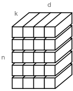
(a)

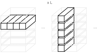
(b)

(c)

Figure 1: Model architecture. (a) Our model maps the input to a three dimensional tensor of shape $n\times d\times k$ and remains permutation in- and equivariant over axes $n$ and $d$, respectively. (b) Each of the $L$ layers first self-attends over axis $d$ and then over $n$, sharing parameters across the other axis. (c) The inner product of two variables’ representations models the probability of a direct causal effect.

In the following, we show how to parameterize $f_{\phi}$ as a neural network that encodes these properties. After first mapping each $\smash{o^{i}_{j}}$ to a real-valued vector using a position-wise linear layer, $f_{\phi}$ operates over a continuous, three-dimensional tensor of $n$ rows for the observations, $d$ columns for the variables, and feature size $k$. Figure 1 illustrates the key components of the architecture.

Attending over axes $d$ and $n$ The core of $f_{\phi}$ is composed of $L=8$ identical layers. Each layer consists of four residual sublayers, where the first and third apply multi-head self-attention and the second and fourth position-wise feed-forward networks, similar to the Transformer encoder (Vaswani et al., , 2017). To enable information flow across all $n\times d$ tokens of the representation, the model alternates in attending over the observation and the variable dimension (Kossen et al., , 2021). Specifically, the first self-attention sublayer attends over axis $d$, treating axis $n$ as a batch dimension; the second attends over axis $n$, treating axis $d$ as a batch dimension. Since modules are shared across non-attended axes, the representation is permutation equivariant over axes $n$ and $d$ at all times (Lee et al., 2019b, ).

Variational parameters After building up a representation tensor from the input using the attention layers, we max-pool over the observation axis $n$ to obtain a representation $(\mathbf{z}^{1},\dots,\mathbf{z}^{d})$ consisting of one vector $\mathbf{z}^{i}\in\mathbb{R}^{k}$ for each causal variable. Following Lorch et al., (2021), we use two position-wise linear layers to map each $\mathbf{z}^{i}$ to two embeddings $\mathbf{u}^{i},\mathbf{v}^{i}\in\mathbb{R}^{k}$, which are $\ell_{2}$ normalized. We then model the probability of each edge in the causal graph with an inner product:

$$\theta_{i,j}=\sigma\big{(}\tau\,\mathbf{u}^{i}\cdot\mathbf{v}^{j}+b\big{)}$$ (6)

where $\sigma$ is the logistic function, $b$ a learned bias, and $\tau$ a positive scale that is learned in $\log$ space. Since max-pooling is invariant to permutations and since (6) permutes with respect to axis $d$, $f_{\phi}$ satisfies the required permutation invariance over axis $n$ and permutation equivariance over axis $d$.

4.3 Acyclicity

Cyclic causal effects often occur, e.g., when modeling stationary distributions of dynamical systems, and thus loops in a causal structure are possible. However, certain domains may be more accurately modeled by acyclic structures (Rubenstein et al., , 2017). While the variational family in (5) cannot enforce it, we can optimize for acyclicity through $\phi$. Whenever the acyclicity prior is justified, we amend the optimization problem in (2) with the constraint that $q$ only models acyclic graphs in expectation:

$$\mathcal{F}(\phi):=\mathbb{E}_{p(D)}\left[h(f_{\phi}(D))\right]=0$$ (7)

The function $h$ is zero if and only if the predicted edge probabilities induce an acyclic graph. We use the insight by Lee et al., 2019a , who show that acyclicity is equivalent to the spectral radius $\rho$, i.e., the largest absolute eigenvalue, of the predicted matrix being zero. We use power iteration to approximate and differentiate through the largest eigenvalue of $f_{\phi}(D)$ (Golub and Van der Vorst, , 2000; Lee et al., 2019a, ):

$$h(W):=\rho(W)\approx\frac{\mathbf{a}^{\top}W\mathbf{b}}{\mathbf{a}^{\top}\mathbf{b}}~{}~{}~{}\text{where for $t$ steps: }~{}~{}~{}\begin{aligned} \mathbf{a}&\leftarrow\mathbf{a}^{\top}W~{}/~{}\lVert\mathbf{a}^{\top}W\rVert_{2}\\ \mathbf{b}&\leftarrow W\mathbf{b}~{}/~{}\lVert W\mathbf{b}\rVert_{2}\end{aligned}$$ (8)

and $\mathbf{a},\mathbf{b}\in\mathbb{R}^{d}$ are initialized randomly. Since a few steps $t$ are sufficient in practice, (8) scales with $O(d^{2})$ and is significantly more efficient than $O(d^{3})$ constraints based on matrix powers (Zheng et al., , 2018; Yu et al., , 2019). We do not backpropagate gradients with respect to $\phi$ through $\mathbf{a},\mathbf{b}$.

4.4 Optimization

Algorithm 1 Training the inference model $f_{\phi}$

  Parameters: $\phi$ variational, $\lambda$ dual, $\eta$ step size

  while not converged do

     for $l$ steps do

        $\Delta\phi\propto\nabla_{\phi}\big{(}\mathcal{L}(\phi)-\lambda\mathcal{F}(\phi)\big{)}$

     $\lambda\leftarrow\lambda+\eta\mathcal{F}(\phi)$

Combining the objective in (3) with our inference model (5), we can directly use stochastic optimization to train the parameters $\phi$ of the inference model. The expectations over $p(G,D)$ inside $\mathcal{L}$ and $\mathcal{F}$ are approximated using samples from the data-generating process of the domain. When enforcing acyclicity, causal discovery algorithms often use the augmented Lagrangian method for constrained optimization (e.g., Zheng et al., 2018; Brouillard et al., 2020). In this work, we optimize the parameters $\phi$ of a neural network, so we rely on methods specifically tailored for deep learning and solve the constrained program $\max_{\phi}\mathcal{L}(\phi)$ s.t. $\mathcal{F}(\phi)=0$ through its dual formulation (Nandwani et al., , 2019):

$$\begin{split}\min_{\lambda}\max_{\phi}~{}\mathcal{L}(\phi)-\lambda\mathcal{F}(\phi)\end{split}$$ (9)

Algorithm 1 summarizes the general optimization procedure for $q_{\phi}$, which converges to a local optimum under regularity conditions on the learning rates (Jin et al., , 2020). Without an acyclicity constraint, training reduces to the primal updates of $\phi$ with $\lambda=0$.

5 Experimental Setup

Evaluating causal discovery algorithms is difficult since there are few interesting real-world datasets that come with ground-truth causal structure. Often, the believed ground truths may be incomplete or change as expert knowledge improves (Schaffter et al., , 2011; Mooij et al., , 2020). Following prior work, we deal with this difficulty by evaluating our approach using simulated data with known causal structure and by controlling for various aspects of the task. In Appendix E, we additionally report results on a real-world proteomics dataset (Sachs et al., , 2005).

5.1 Domains and Simulated Components

We study three domains: two classes of structural causal models (SCMs) as well as semisynthetic single-cell expression data of gene regulatory networks (GRNs). To study the generalization of AVICI beyond the training distribution $p(D)$, we carefully construct a spectrum of test distributions $\tilde{p}(D)$ that incur substantial shift from $p(D)$ in terms of the causal structures, mechanisms, and noise, which we study in various combinations. Whenever we consider interventional data in our experiments, half of the dataset consists of observational data and half of single-variable interventions.

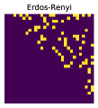
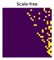
(a)

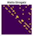
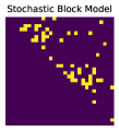
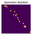
(b)

(c)

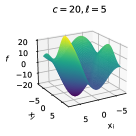
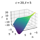
(d)

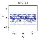
(e)

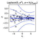
(f)

(a)                                                        (b)                                  (c)

Figure 3: Moving out-of-distribution in the Rff domain. Randomly sampled data-generating components of the nonlinear SCM domain during training $p(D)$ (top) and o.o.d. evaluation $\tilde{p}(D)$ (bottom). For visualization, the adjacency matrices (a) are topologically sorted, the causal mechanisms (b) have two parents, where $c$ and $\ell$ are output and length scales of the underlying GP, and the noise (c) is shown as a function of one parent, where dashed lines indicate $0.66$, $0.95$, and $0.999$ coverage.

Data-generating processes $p(D\,|\,G)$  We consider SCMs with linear functions (Linear) and with nonlinear functions of random Fourier features (Rff) that correspond to functions drawn from a Gaussian process with squared exponential kernel (Rahimi and Recht, , 2007). In the out-of-distribution (o.o.d.) setting $\tilde{p}(D)$, we sample the linear function and kernel parameters from the tails of $p(D)$ and unseen value ranges. Moreover, we simulate homoscedastic Gaussian noise in the training distribution $p(D)$ but test on heteroscedastic Cauchy and Laplacian noise o.o.d. that is induced by randomly drawn, nonlinear functions $h_{j}$. In Linear and Rff, interventions set variables to random values and are performed on a subset of target variables containing half of the nodes.

In addition to SCMs, we consider the challenging domain of GRNs (Grn) using the simulator of Dibaeinia and Sinha, (2020). Contrary to SCMs, gene expression samples correspond to draws from the steady state of a stochastic dynamical system that varies between cell types (Huynh-Thu and Sanguinetti, , 2019). In the o.o.d. setting, the parameters sampled for the Grn simulator are drawn from significantly wider ranges. In addition, we use the noise levels of different single-cell RNA sequencing technologies, which were calibrated on real datasets. In Grn, interventions are performed on all nodes and correspond to gene knockouts, forcing the transcription rate of a variable to zero.

Causal structures $p(G)$ Following prior work, we use random graph models and known biological networks to sample ground-truth causal structures. In all three domains, the training data distribution $p(D)$ is induced by simple Erdős-Rényi and scale-free graphs (Erdős and Rényi, , 1959; Barabási and Albert, , 1999). In the o.o.d. setting, $\tilde{p}(D)$ of the Linear and Rff domains are simulated using causal structures from the Watts-Strogatz model, capturing small-world phenomena (Watts and Strogatz, , 1998); the stochastic block model, generalizing Erdős-Rényi to community structures (Holland et al., , 1983); and geometric random graphs, modeling connectivity based on spatial distance (Gilbert, , 1961). In the Grn domain, we use subgraphs of the known S. cerevisiae and E. coli GRNs and their effect signs whenever known. To extract these subgraphs, we use the procedure by Marbach et al., (2009) to maintain structural patterns like motifs and modularity (Ravasz et al., , 2002; Shen-Orr et al., , 2002).

To illustrate the distribution shift from $p(D)$ to $\tilde{p}(D)$, Figure 3 shows a set of graph, mechanism, and noise distribution samples in the Rff domain. In Appendix A, we give the detailed parameter configurations and functions defining $p(D)$ and $\tilde{p}(D)$ in the three domains. We also provide details on the simulator by Dibaeinia and Sinha, (2020) and subgraph extraction (Marbach et al., , 2009).

5.2 Evaluation Metrics

All experiments throughout this paper are conducted on datasets that AVICI has never seen during training, regardless of whether we evaluate the predictive performance in-distribution or o.o.d. To assess how well a predicted structure reflects the ground truth, we report the structural Hamming distance (SHD) and the structural intervention distance (SID) (Peters and Bühlmann, , 2015). While the SHD simply reflects the graph edit distance, the SID quantifies the closeness of two graphs in terms of their interventional adjustment sets. For these metrics and for single-edge precision, recall, and F1 score, we convert the posterior probabilities predicted by AVICI to hard predictions using a threshold of $0.5$. We evaluate the uncertainty estimates by computing the areas under the precision-recall curve (AUPRC) and the receiver operating characteristic (AUROC) (Friedman and Koller, , 2003). How well these uncertainty estimates are calibrated is quantified with the expected calibration error (ECE) (DeGroot and Fienberg, , 1983). More details on the metrics are given in Appendix B.

5.3 Inference Model Configuration

We train three inference models overall, one for each domain, and perform all experiments on these three trained models, both when predicting from only observational and from interventional data. During training, the datasets sampled from $p(D)$ have $d=2$ to $50$ variables and $n=200$ samples. With probability 0.5, these training datasets contain $50$ interventional samples. The inference models in the three domains share identical hyperparameters for the architecture and optimization, except for the dropout rate. We add the acyclicity constraint for the SCM domains Linear and Rff. Details on the optimization and architecture are given in Appendix C.

6 Experimental Results

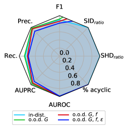
(a)

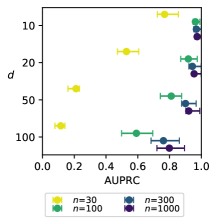
(b)

(a) Linear

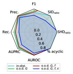
(b)

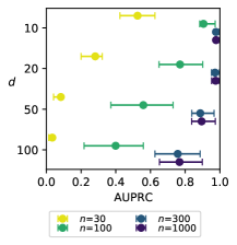
(c)

(b) Rff

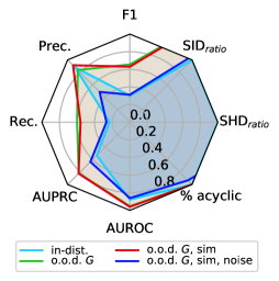
(c)

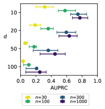
(d)

(c) Grn

Figure 5: Generalization properties of the inference model $f_{\phi}$. Top row plots show performance metrics of AVICI under increasing distributional shift given $n$ $=$ $1000$ observations for $d$ $=$ $30$ variables. $\text{SID}_{\text{ratio}}$ is defined as $\text{SID}_{\text{in-dist.}}/\text{SID}$ and analogously for SHD. Thus, higher is better for all metrics. Bottom row shows the in-distribution AUPRC for various $d$ as we vary the number of observations provided to AVICI. The datasets contain interventional data (cf. Section 5.1). All values are the mean over fifteen random task instances. Error bars indicate the interquartile range.

6.1 Out-Of-Distribution Generalization

Sensitivity to distribution shift In our first set of experiments, we study the generalization capabilities of our inference models across the spectrum of test distributions described in Section 5.1. We perform causal discovery from $n=1000$ observations in systems of $d=30$ variables. Starting from the training distribution $p(D)$, we incrementally introduce the described distribution shifts in the causal structures, causal mechanisms, and finally noise, where fully o.o.d. corresponds to $\tilde{p}(D)$. The top row of Figure 5 visualizes the results of an empirical sensitivity analysis. The radar plots disentangle how combinations of the three o.o.d. aspects, i.e., graphs, mechanisms, and noise, affect the empirical performance in the three domains Linear, Rff, and Grn. In addition to the metrics in Section 5.2, we also report the percentage of predicted graphs that are acyclic.

In the Linear domain, AVICI performs very well in all metrics and hardly suffers under distribution shift. In contrast, Grn is the most challenging problem domain and the performance degrades more significantly for the o.o.d. scenarios. We observe that AVICI can perform better under certain distribution shifts than in-distribution, e.g., in Grn. This is because AVICI empirically performs better at predicting edges adjacent to large-degree nodes, a common feature of the E. coli and S. cerevisiae graphs not present in the Erdős-Rényi training structures. We also find that acyclicity is perfectly satisfied for Linear and Rff and that AUPRC and AUROC do not suffer as much from distributional shift as the metrics based on thresholded point estimates.

In Appendix E.1, we additionally report results for generalization from Linear to Rff and vice versa, i.e., to entirely unseen function classes of causal mechanisms in addition to the previous o.o.d. shifts.

Generalization to unseen problem sizes In addition to the sensitivity to distribution shift, we study the ability to generalize to unseen problem sizes. The bottom row of Figure 5 illustrates the AUPRC for the edge predictions of AVICI when varying $d$ and $n$ on unseen in-distribution data. The predictions improve with the number of data points $n$ while exhibiting diminishing marginal improvement when seeing additional data. Moreover, the performance decreases smoothly as the number of variables $d$ increases and the task becomes harder. Most importantly, this robust behavior can be observed well beyond the settings used during training ($n=200$ and $d\leq 50$).

6.2 Benchmarking

Table 1: Benchmarking results ($d=30$ variables). Mean SID ($\downarrow$) and F1 score ($\uparrow$) with standard error of all methods on $30$ random task instances. Methods in the top section use only observational data, in the bottom section both observational and interventional data. We highlight the best result of each section and those within its $95$% confidence interval according to an unequal variances $t$-test.

Linear Rff Grn Algorithm SID F1 SID F1 SID F1 GES 215.6  (35.0) 0.548  (0.03) 346.3  (44.4) 0.285  (0.03) 573.6  (29.2) 0.058  (0.01) LiNGAM 413.4  (48.4) 0.369  (0.04) 410.3  (47.6) 0.238  (0.02) 617.5  (31.7) 0.044  (0.01) PC 400.5  (53.7) 0.338  (0.03) 370.1  (51.2) 0.421  (0.03) 594.0  (30.0) 0.061  (0.01) DAG-GNN 474.5  (50.8) 0.154  (0.01) 425.3  (50.2) 0.221  (0.03) 588.7  (36.6) 0.078  (0.02) GraN-DAG 466.0  (54.3) 0.200  (0.03) 328.6  (48.4) 0.476  (0.05) 582.4  (33.4) 0.073  (0.02) AVICI (ours) 145.6  (21.5) 0.672  (0.04) 255.1  (48.2) 0.618  (0.06) 641.7  (34.7) 0.000  (0.00) GIES 120.8  (26.2) 0.736  (0.03) 304.8  (44.0) 0.338  (0.04) 545.5  (26.9) 0.092  (0.01) IGSP 244.0  (34.4) 0.559  (0.02) 374.1  (45.0) 0.407  (0.04) 597.4  (31.7) 0.057  (0.01) DCDI 383.5  (45.1) 0.327  (0.03) 282.8  (46.3) 0.409  (0.04) 590.9  (30.6) 0.075  (0.02) AVICI (ours) 110.9  (19.3) 0.819  (0.02) 192.7  (44.8) 0.707  (0.06) 416.9  (47.1) 0.338  (0.06)

Next, we benchmark AVICI against existing algorithms. Using only observational data, we compare with the PC algorithm (Spirtes et al., , 2000), GES (Chickering, , 2003), LiNGAM (Shimizu et al., , 2006), DAG-GNN (Yu et al., , 2019), and GraN-DAG (Lachapelle et al., , 2020). Mixed with interventional data, we compare with GIES (Hauser and Bühlmann, , 2012), IGSP (Wang et al., , 2017), and DCDI (Brouillard et al., , 2020). We tune the important hyperparameters of each baseline on held-out task instances of each domain. When computing the evaluation metrics, we favor methods that only predict (interventional) Markov equivalence classes by orienting undirected edges correctly when present in the ground truth. Details on the baselines are given in Appendix D.

The benchmarking is performed on the fully o.o.d. domain distributions $\tilde{p}(D)$, i.e., under distribution shifts on causal graphs, mechanisms, and noise distributions w.r.t. the training distribution of AVICI. Table 1 shows the SID and F1 scores of all methods given $n$ $=$ $1000$ observations for $d$ $=$ $30$ variables. We find that the AVICI model trained on Linear outperforms all baselines, both given observational or interventional data, despite operating under significant distribution shift. Only GIES achieves comparable accuracy. The same holds for Rff, where GraN-DAG and DCDI perform well but ultimately do not reach the accuracy of AVICI.

In the Grn domain, where inductive biases are most difficult to specify, classical methods fail to infer plausible graphs. However, provided interventional data, AVICI can use its learned inductive bias to infer plausible causal structures from the noisy gene expressions, even under distribution shift. This is a promising step towards reliable structure discovery in fields like molecular biology. Even without gene knockout data, AVICI achieves nontrival AUROC and AUPRC while classical methods predict close to randomly (Table 9 in Appendix E; see also Dibaeinia and Sinha, 2020; Chen and Mar, 2018).

Results for in-distribution data and for larger graphs of $d$ $=$ $100$ variables are given in Appendices E.2 and E.3. In Appendix E.4, we also report results for a real proteomics dataset (Sachs et al., , 2005).

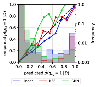
(a)

Linear Rff Grn GES^∗ 0.031  (0.00) 0.068  (0.02) 0.092  (0.01) LiNGAM^∗ 0.066  (0.02) 0.054  (0.01) 0.053  (0.01) PC^∗ 0.036  (0.00) 0.033  (0.01) 0.065  (0.01) DAG-GNN^∗ 0.078  (0.01) 0.063  (0.01) 0.063  (0.01) GraN-DAG^∗ 0.046  (0.01) 0.042  (0.01) 0.199  (0.05) AVICI (ours) 0.013  (0.00) 0.024  (0.01) 0.018  (0.00) GIES^∗ 0.027  (0.00) 0.074  (0.02) 0.094  (0.01) IGSP^∗ 0.042  (0.01) 0.083  (0.01) 0.077  (0.01) DCDI^∗ 0.068  (0.01) 0.087  (0.02) 0.170  (0.03) DiBS 0.056  (0.02) 0.035  (0.01) 0.093  (0.01) AVICI (ours) 0.011  (0.00) 0.022  (0.01) 0.024  (0.01) $*$ Nonparametric DAG bootstrap (Friedman et al., , 1999) (b)

Figure 5: Uncertainty calibration ($d=30$ variables). As previously, datasets are held-out and o.o.d. in terms of graph, parameters, and noise. (a) Calibration plots for AVICI aggregating the predictions for ten test cases of each domain. The histograms on the right $y$-axis show the frequency of predictions at each confidence level. (b) ECE ($\downarrow$) with standard error averaged over ten test cases. Methods in the top (bottom) section use observational (and interventional) data. We highlight the best result and those within its $95$% confidence interval according to an unequal variances $t$-test.

Uncertainty quantification Using metrics of calibration, we can evaluate the degree to which predicted edge probabilities are consistent with empirical edge frequencies (DeGroot and Fienberg, , 1983; Guo et al., , 2017). We say that a predicted probability $\smash{p}$ is calibrated if we empirically observe an event in $\smash{(p\cdot 100)\%}$ of the cases. When plotting the observed edge frequencies against their predicted probabilities, a calibrated algorithm induces a diagonal line. The expected calibration error (ECE) represents the weighted average deviation from this diagonal. For further details, see Appendix B.

Since the baseline algorithms only infer point estimates of the causal structure, we use the nonparametric DAG bootstrap to estimate edge probabilities (Friedman et al., 1999, Appendix D). We additionally compare AVICI with DiBS, which infers Bayesian posterior edge probabilities like AVICI (Lorch et al., , 2021). Figure 5 gives the calibration plots for AVICI and Table 5b the ECE for all methods. In each domain, the marginal edge probabilities predicted by AVICI are the most calibrated in terms of ECE. Moreover, Figure 5a shows that AVICI closely traces the perfect calibration line, which highlights its accurate uncertainty calibration across the probability spectrum.

In Appendix E.5, we additionally report AUROC and AUPRC metrics for all methods. We also provide calibration plots analogous to Figure 5 for the baselines (Figure 8), which often show vastly overconfident predictions where the calibration line is far below the diagonal.

6.3 Ablations

Finally, we analyze the importance of key architecture components of the inference network $\smash{f_{\phi}}$. Focusing on the Rff domain, we train several additional models and ablate single architecture components. We vary the network depth $L$, the axes of attention, the representation of $\theta$, and the number of training steps for $\phi$. All other aspects of the model, training and data simulation remain unchanged.

Table 2 summarizes the results. Most noticeably, we find that the performance drops significantly when attending only over axis $d$ and aggregating information over axis $n$ only once through pooling after the $2L$ self-attention layers. Attending only over axis $n$ is not sensible since variable interactions are not processed until the prediction of $\theta$, but we still include the results for completeness.

We also test an alternative variational parameter model given by $\smash{\theta_{i,j}=\phi^{\top}_{\theta}\tanh\left(\phi_{u}^{\top}\mathbf{u}^{i}+\phi_{v}^{\top}\mathbf{v}^{j}\right)}$ that uses an additional, learned vector $\smash{\phi_{\theta}}$ and matrices $\smash{\phi_{u},\phi_{v}}$. This model has been used in related causal discovery work for searching over high-scoring causal DAGs (Zhu et al., , 2020) and is a relational network (Santoro et al., , 2017). This variant also satisfies permutation equivariance (cf. Section 4.2) since it applies the same MLP elementwise to each edge pair $[\mathbf{u}^{i},\mathbf{v}^{j}]$. Ultimately, we find no statistically significant difference in performance to our simpler model in Eq. (6), hence we opt for less parameters and a lower memory requirement.

Lastly, Table 2 shows that the causal discovery performance of AVICI scales up monotonically with respect to network depth and training time. Even substantially smaller models of $L$ $=$ $4$ or shorter training times achieve an accuracy that is on par with most baselines (cf. Table 1). Our main models ($\star$) have a moderate size of $4.2$ $\times$ $10^{6}$ parameters, which amounts to only $17.0$ MB at f$32$ precision. Performing causal discovery (computing a forward pass) given on a trained model takes only a few seconds on CPU.

Table 2: Ablations of the architecture of $f_{\phi}$. Models are evaluated on $100$ interventional datasets of $d=30$ variables in the Rff domain. Top row ($\star$) corresponds to the model used in the main experiments. In (a), we vary the number of blocks $L$; in (b), the axes over which attention is performed; in (c), the generative model of the variational parameters; in (d), the number of update steps of $\phi$. We again highlight the best result and those within its $95$% $t$-test confidence interval.

Rff (in-dist.) Rff (o.o.d.) $L$ ax. $d$ ax. $n$ $\theta$ model steps SID AUPRC SID AUPRC ($\star$) 8 ✓ ✓ Eq. (6) 300k 65.2  (8.4) 0.972  (0.00) 221.5  (24.7) 0.650  (0.03) (a) 1 267.2  (22.0) 0.635  (0.01) 394.2  (28.4) 0.242  (0.02) 2 195.9  (18.5) 0.825  (0.01) 343.1  (27.1) 0.400  (0.03) 4 116.6  (13.1) 0.937  (0.01) 264.0  (24.8) 0.566  (0.03) (b) ✓ 351.5  (27.9) 0.552  (0.01) 414.2  (29.5) 0.209  (0.02) ✓ 416.8  (29.6) 0.256  (0.01) 390.2  (27.6) 0.078  (0.01) (c) (Santoro et al., , 2017) 72.4  (9.2) 0.971  (0.00) 225.7  (25.2) 0.634  (0.03) (d) 100k 96.9  (11.6) 0.955  (0.00) 259.3  (26.6) 0.589  (0.04)

7 Discussion

We proposed AVICI, a method for inferring causal structure by performing amortized variational inference over an arbitrary data-generating distribution. Our approach leverages the insight that inductive biases crucial for statistical efficiency in structure learning might be more easily encoded in a simulator than in an inference technique. This is reflected in our experiments, where AVICI solves structure learning problems in complex domains intractable for existing approaches (Dibaeinia and Sinha, , 2020). Our method can likely be extended to other typically difficult domains, including settings where we cannot assume causal sufficiency (Bhattacharya et al., , 2021). Our approach will continually benefit from ongoing efforts in developing (conditional) generative models and domain simulators.

Using AVICI still comes with several trade-offs. First, while optimizing the dual program empirically induces acyclicity, this constraint is not satisfied with certainty using the variational family considered here. Moreover, similar to most amortization techniques (Amos, , 2022), AVICI gives no theoretical guarantees of performance. Some classical methods can do so in the infinite sample limit given specific assumptions on the data-generating process (Peters et al., , 2017). However, future work might obtain guarantees for AVICI that are similar to learning theory results for the bivariate causal discovery case (Lopez-Paz et al., , 2015).

Our experiments demonstrate that our inference models are highly robust to distributional shift, suggesting that the trained models could be useful out-of-the-box in causal structure learning tasks outside the domains studied in this paper. In this context, fine-tuning a pretrained AVICI model on labeled real-world datasets is a promising avenue for future work. To facilitate this, our code and models are publicly available at: https://github.com/larslorch/avici.

Appendix A Domain Specification and Simulation

In this section, we define the training and test distributions $p(D)$ and $\tilde{p}(D)$ concretely in terms of the parameters and notation introduced in the main text. Based on these definitions, Table 3 summarizes all parameters of the data-generating processes for Linear and Rff and specifies how they are sampled for a random task instance. Table 4 lists the same specifications for the Grn domain. The notation and parameters are defined in the following subsections.

Table 3: Specification of the training and out-of-distribution data-generating processes $p(D)$ and $\tilde{p}(D)$ for the Linear and Rff domain. All specifications except the mechanism function type are the same for the two domains. For each random task instance, the parameter configurations are sampled uniformly randomly from all possible combinations of the sets of options. The graph model classes are sampled in equal proportions out-of-distribution. Empty fields indicate that the component is not part of the distribution.

In-distribution $p(D)$ Out-of-distribution $\tilde{p}(D)$ Graph Erdős-Rényi expected edges/node $\in\{1,2,3\}$ Scale-free (in-degree) edges/node $\in\{1,2,3\}$ attach. power $\alpha$ $\in\{1.0\}$ Scale-free (out-degree) edges/node $\in\{1,2,3\}$ edges/node $\in\{2\}$ attach. power $\alpha$ $\in\{1.0\}$ attach. power $\alpha$ $\in\{0.5,1.5\}$ Watts-Strogatz lattice dim. $k$ $\in\{2,3\}$ rewire prob. $\in\{0.3\}$ Stochastic Block Model expected edges/node $\in\{2\}$ blocks $\in\{5,10\}$ damp. inter-block prob. $\in\{0.1\}$ Geometric Random Graphs radius $\in\{0.1\}$ Mechanism Linear function${}^{\text{(a)}}$ weights $\mathbf{w}$ $\sim\text{Unif}_{\pm}(1,3)$ weights $\mathbf{w}$ $\sim\text{Unif}_{\pm}(0.5,2)$ $\sim\text{Unif}_{\pm}(2,4)$ bias $b$ $\sim\text{Unif}(-3,3)$ bias $b$ $\sim\text{Unif}(-3,3)$ Random Fourier function${}^{\text{(b)}}$ SE length scale $\ell$ $\sim\text{Unif}(7,10)$ SE length scale $\ell$ $\sim\text{Unif}(5,8)$ $\sim\text{Unif}(8,12)$ SE output scale $c$ $\sim\text{Unif}(10,20)$ SE output scale $c$ $\sim\text{Unif}(8,12)$ $\sim\text{Unif}(18,22)$ bias $b$ $\sim\text{Unif}(-3,3)$ bias $b$ $\sim\text{Unif}(-3,3)$ Noise (indiv. per variable) $\mathcal{N}(0,\sigma^{2})$ $\sigma$ $\sim\text{Unif}(0.2,2)$ $\text{Laplace}(0,\sigma^{2})$ $\sigma^{2}(\mathbf{x}_{\text{pa}_{j}})$ (heterosced.) $\sim p(h_{\text{rff}})$ $\text{Cauchy}(0,\sigma^{2})$ $\sigma^{2}(\mathbf{x}_{\text{pa}_{j}})$ (heterosced.) $\sim p(h_{\text{rff}})$ Interventions Target nodes random 50% of nodes random 50% of nodes Intervention values $x_{j}$ $\sim\text{Unif}_{\pm}(1,3)$ $x_{j}$ $\sim\text{Unif}_{\pm}(1,5)$ (a) Only Linear domain (b) Only Rff domain Aliases: – $\text{Unif}_{\pm}(a,b)$: uniform mixture of $\text{Unif}(a,b)$ and $\text{Unif}(-b,-a)$ – $p(h_{\text{rff}})$: distribution over heteroscedastic noise scale functions, induced by the squash function $h_{\text{rff}}(\mathbf{x})=\log(1+\exp(g_{\text{rff}}(\mathbf{x}))$ and random Fourier feature functions $g_{\text{rff}}(\mathbf{x})$ with SE length scale $\ell=10$ and output scale $c=2$ (cf. Rff domain)

Table 4: Specification of the training and out-of-distribution data-generating processes $p(D)$ and $\tilde{p}(D)$ for the Gene domain. For each random task instance, the parameter configurations are sampled uniformly randomly from all possible combinations of the sets of options. The graph model classes are sampled in equal proportions out-of-distribution. Empty fields indicate that the component is not part of the distribution.

In-distribution $p(D)$ Out-of-distribution $\tilde{p}(D)$ Graph Erdős-Rényi expected edges/node $\in\{1,2,3\}$ Scale-free (out-degree) edges/node $\in\{1,2,3\}$ attach. power $\alpha$ $\in\{0.5,0.8,1.0,1.2,1.5\}$ E. coli subgraph top-$p$ perc. modular $\in\{0.2\}$ (Marbach et al., , 2009) S. cerevisiae subgraph top-$p$ perc. modular $\in\{0.2\}$ (Marbach et al., , 2009) Mechanism GRN simulator no. cell types $\in\{5\}$ no. cell types $\in\{10\}$ (Dibaeinia and Sinha, , 2020) decay rates $\lambda$ $\in\{0.7,0.8,0.9\}$ decay rates $\lambda$ $\in\{0.5,1.5\}$ system noise scale $\xi$ $\in\{0.9,1.0,1.1\}$ system noise scale $\xi$ $\in\{0.5,1.5\}$ Hill function coeff. $\gamma$ $\in\{1.9,2.0,2.1\}$ Hill function coeff. $\gamma$ $\in\{1.5,2.5\}$ MR prod. rate $b$ $\sim\text{Unif}(1,3)$ MR prod. rate $b$ $\sim\text{Unif}(0.5,2)$ $\sim\text{Unif}(2,4)$ interactions $k$ $\sim\text{Unif}(1,5)$ interactions $k$ $\sim\text{Unif}(1,3)$ $\sim\text{Unif}(3,7)$ $\text{signs}(k)$ per node $\sim\text{Bern}(p)$ where $p$ $\text{signs}(k)$ per node from E. coli      $\sim\text{Beta}(1,1)$ or $\sim\text{Bern}(p)$      $\sim\text{Beta}(0.5,0.5)$ (cf. Sec. A.1.2) Measurement Noise Platform^† 10X chromium $p_{\text{outlier}}\in\{0.01\}$ $\mu_{\text{outlier}}\in\{3.0,5.0\}$ $\sigma_{\text{outlier}}\in\{1.0\}$ $\mu_{\text{lib}}\in\{4.5,6.0\}$ $\sigma_{\text{lib}}\in\{0.3,0.4,0.7\}$ $\delta\in\{45,74,82\}$ $\tau\in\{8.0\}$ Illumina HiSeq2000 $p_{\text{outlier}}\in\{0.01\}$ $\mu_{\text{outlier}}\in\{0.8\}$ $\sigma_{\text{outlier}}\in\{1.0\}$ $\mu_{\text{lib}}\in\{7.0\}$ $\sigma_{\text{lib}}\in\{0.4\}$ $\delta\in\{80\}$ $\tau\in\{8.0\}$ Drop-seq $p_{\text{outlier}}\in\{0.01\}$ $\mu_{\text{outlier}}\in\{3.0\}$ $\sigma_{\text{outlier}}\in\{1.0\}$ $\mu_{\text{lib}}\in\{4.4\}$ $\sigma_{\text{lib}}\in\{0.8\}$ $\delta\in\{85\}$ $\tau\in\{8.0\}$ Smart-seq $p_{\text{outlier}}\in\{0.01\}$ $\mu_{\text{outlier}}\in\{4.5\}$ $\sigma_{\text{outlier}}\in\{1.0\}$ $\mu_{\text{lib}}\in\{10.8\}$ $\sigma_{\text{lib}}\in\{0.55\}$ $\delta\in\{92\}$ $\tau\in\{2.0\}$ Interventions Target nodes all nodes all nodes Intervention type gene knockout gene knockout $\dagger$ Noise specifications were collected from calibrations performed by Dibaeinia and Sinha, (2020) on real datasets generated by the different scRNA-seq platforms.

A.1 Causal Structures

A.1.1 Random graph models

In Erdős-Rényi graphs, each edge is sampled independently with a fixed probability (Erdős and Rényi, , 1959). We scale this probability to obtain $O(d)$ edges in expectation. Scale-free graphs are generated by a sequential preferential attachment process, where in- or outgoing edges of node $i$ to the previous $i-1$ nodes are sampled with probability $\propto$ $\text{deg}(j)^{\alpha}$ (Barabási and Albert, , 1999). Watts-Strogatz graphs are $k$-dimensional lattices, whose edges get rewired globally to random nodes with a specified probability (Watts and Strogatz, , 1998). The stochastic block model generalizes Erdős-Rényi to capture community structure. Splitting the nodes into a random partition of so-called blocks, the inter-block edge probability is dampened by a multiplying factor compared to the intra-block probability, also tuned to result in $O(d)$ edges in expectation (Holland et al., , 1983). Lastly, geometric random graphs model connectivity based on two-dimensional Euclidian distance within some radius, where nodes are randomly placed inside the unit square (Gilbert, , 1961).

For undirected random graph models, we orient edges by selecting the upper-triangular half of the adjacency matrix. The classes of random graph models are sampled in equal proportion when generating a set of evaluation datasets (Tables 3 and 4).

A.1.2 Subgraph Extraction from Real-World Networks

For the evaluation in the Grn domain, we sample realistic causal graphs by extracting subgraphs from the known E. coli and S. cerevisiae regulatory networks. For this, we rely on the procedure by Marbach et al., (2009), which is also used by Schaffter et al., (2011) and Dibaeinia and Sinha, (2020). Their graph extraction method is carefully designed to capture the structural properties of biological networks by preserving the functional and structural properties of the source network.

Algorithm

The procedure extracts a random subgraph of the source network by selecting a subset of nodes $\mathcal{V}$, and then returning the graph containing all edges from the source network covered by $\mathcal{V}$. Starting from a random seed node, the algorithm proceeds by iteratively adding new nodes to $\mathcal{V}$. In each step, this new node is selected from the set of neighbors of the current set $\mathcal{V}$. The neighbor to be added is selected greedily such that the resulting subgraph has maximum modularity (Marbach et al., , 2009).

To introduce additional randomness, Marbach et al., (2009) propose to randomly draw the new node from the set of neighbors inducing the top-$p$ percent of the most modular graphs. In our experiments, we adopt the latter with $p=20$ percent, similar to Schaffter et al., (2011). The original method of Marbach et al., (2009) is intended for undirected graphs. Thus, we use the undirected skeleton of the source network for the required modularity and neighborhood computation.

Real GRNs

We take the E. coli and S. cerevisiae regulatory networks as provided by the GeneNetWeaver repository, which have $1565$ and $4441$ nodes (genes), respectively. For E. coli, we also know the true signs of a large proportion of causal effects. When extracting a random subgraph from E. coli, we take the true signs of the effects and map them onto the randomly sampled interaction terms $k\in\mathbb{R}^{d\times d}$ used by SERGIO; cf. Section A.2.2. When the interaction signs are unknown or uncertain in E. coli, we impute a random sign in the interaction terms $k$ of SERGIO based on the frequency of known positive and negative signs in the E. coli graph.

Empirically, individual genes in E. coli tend to predominantly have either up- or down-regulating effects on their causal children. To capture this aspect in S. cerevisiae also, we fit the probability of an up-regulating effect caused by a given gene in E. coli to a Beta distribution. For each node $j$ in an extracted subgraph of S. cerevisiae, we draw a probability $p_{j}$ from this Beta distribution and then sample the effect signs for the outgoing edges of node $j$ using $p_{j}$. As a result, the genes in the subgraphs of S. cerevisiae individually also have mostly up- or down-regulating effects. Maximum likelihood estimation for this Beta distribution yielded $\alpha=0.2588$ and $\beta=0.2499$.

The E. coli and S. cerevisiae graphs and effect signs used in the experiments are taken from the GeneNetWeaver repository (Schaffter et al., , 2011) (MIT License).

A.2 Data-Generating Processes

A.2.1 Structural Causal Models

In the Linear and Rff domains, the data-generating processes are modeled by structural causal models (SCMs). In this work, we consider SCMs with causal mechanisms that model each causal variable $x_{j}$ given its parents $\mathbf{x}_{\text{pa}(j)}$ as

$$x_{j}\leftarrow f_{j}(\mathbf{x}_{\text{pa}(j)},\epsilon_{j})=f_{j}(\mathbf{x}_{\text{pa}(j)})+h_{j}(\mathbf{x}_{\text{pa}(j)})\epsilon_{j}$$ (10)

where the noise $\epsilon_{j}$ is additive and may be heteroscedastic through an input-dependent noise scale $\smash{h_{j}(\mathbf{x}_{\text{pa}(j)})}$. Even in the homogeneous noise setting, the scale of each noise distribution $p(\epsilon_{j})$ is random and thus different for each variable $x_{j}$. We write $\mathbf{x}_{\text{pa}(j)}$ when indexing $\mathbf{x}$ at the parents of node $j$. In the heteroscedastic setting, we parameterize the noise scales as $h_{j}(\mathbf{x})=\log(1+\exp(g_{j}(\mathbf{x}))$ for a set of nonlinear functions $g_{j}$.

Prior to performing inference with AVICI or any baseline, each set of SCM observations $D$ is standardized variable-wise by subtracting its mean and dividing by its standard deviation, so that each $x_{j}$ has mean $0$ and variance $1$, avoiding potential varsortability bias (Reisach et al., , 2021).

In the Linear domain, the functions $f_{j}$ are given by affine transforms

$$f_{j}(\mathbf{x}_{\text{pa}(j)})=\mathbf{w}_{j}^{\top}\mathbf{x}_{\text{pa}(j)}+b_{j}$$ (11)

whose weights $\mathbf{w}_{j}$ and bias $b_{j}$ are sampled independently for each $f_{j}$. In the Rff domain, the functions $f_{j}$ modeling each causal variable $x_{j}$ given its parents $\mathbf{x}_{\text{pa}(j)}$ are drawn from a Gaussian Process

$$f_{j}\sim\mathcal{GP}(b_{j},k_{j})$$ (12)

with bias $b_{j}$ and squared exponential (SE) kernel $k_{j}(\mathbf{x},\mathbf{x}^{\prime})=c_{j}^{2}\exp\left(-\lVert\mathbf{x}-\mathbf{x}^{\prime}\rVert_{2}^{2}/2\ell_{j}^{2}\right)$ with length scale $\ell_{j}$ and output scale $c_{j}$. The parameters $b_{j}$, $c_{j}$, and $\ell_{j}$ are sampled independently for each variable $j$. To obtain explicit function draws $f_{j}$ from the GP, we approximate $f_{j}$ with random Fourier features (Rahimi and Recht, , 2007). Specifically, we can obtain $f_{j}\sim\mathcal{GP}(b_{j},k(\mathbf{x},\mathbf{x}^{\prime}))$ for a SE kernel $k$ with length scale $\ell_{j}$ and output scale $c_{j}$ by sampling

$$f_{j}(\mathbf{x}_{\text{pa}(j)})=b_{j}+c_{j}\,{\sqrt{\tfrac{2}{M}}}\,\sum_{m=1}^{M}\alpha^{(m)}\cos\left(\tfrac{1}{\ell_{j}}\,\bm{\omega}^{(m)}\cdot\mathbf{x}_{\text{pa}(j)}+\delta^{(m)}\right)$$ (13)

with $\alpha^{(m)}\sim\mathcal{N}(0,1)$, $\bm{\omega}^{(m)}\sim\mathcal{N}(0,\mathbf{I})$, and $\delta^{(m)}\sim\text{Unif}(0,2\pi)$. Throughout this work, we use $M$ $=$ $100$. The function draws become faithful GP samples as $M\rightarrow\infty$ (Rahimi and Recht, , 2007). When $x_{j}$ is a root node and thus has no parents, $f_{j}$ is a constant.

A.2.2 Single-Cell Gene Expression Data

In the Grn domain, our goal is to evaluate causal discovery from realistic gene expression data. There exist several models to simulate the mechanisms, intervention types, and technical measurement noise underlying single-cell expression data of gene regulatory networks (Schaffter et al., , 2011; Huynh-Thu and Sanguinetti, , 2019; Dibaeinia and Sinha, , 2020). We use the simulator by Dibaeinia and Sinha, (2020) (SERGIO) because it resembles the data collected by modern high-throughput single-cell RNA sequencing (scRNA-seq) technologies. Related genomics simulators, for example, GeneNetWeaver (Schaffter et al., , 2011), were developed for the simulation of microarray gene expression platforms. In the following, we give an overview of how to simulate scRNA-seq data with SERGIO. Dibaeinia and Sinha, (2020) provide all the details and additional background from the related literature.

Simulation

Given a causal graph over $d$ genes and a specification of the simulation parameters, SERGIO generates a synthetic scRNA-seq dataset $D$ in two stages. The $n$ observations in $D$ correspond to $n$ cell samples, that is, the expressions of the $d$ genes recorded in a single cell corresponds to one row in $D$.

In the first stage, SERGIO simulates clean gene expressions by sampling randomly-timed snapshots from the steady state of a dynamical system. In this regulatory process, the genes are expressed at rates influenced by other genes using the chemical Langevin equation, similar to Schaffter et al., (2011) and (Dibaeinia and Sinha, , 2020). The source nodes in the causal graph $G$ are denoted master regulators (MRs), whose expressions evolve at constant production and decay rates. The expressions of all downstream genes evolve nonlinearly under production rates caused by the expression of their causal parents in $G$. Cell types are defined by specifications of the MR production rates, which significantly influence the evolution of the system. Thus, the dataset contains variation due to biological system noise within collections of cells of the same type and due to different cell types. Ultimately, we generate single-cell samples collected from five to ten cell types (Dibaeinia and Sinha, , 2020).

In the second stage, the clean gene expressions sampled previously are corrupted with technical measurement error that resembles the noise phenomena found in real scRNA-seq data:

• outlier genes: a small set of genes have unusually high expression across measurements

• library size: different cells have different total UMI counts, following a log-normal distribution

• dropouts: a high percentage of genes are recorded with zero expression in a given measurement

• unique molecule identifier (UMI) counts: we observe Poisson-distributed count data rather than the clean expression values

To configure these noise modules, we use the parameters calibrated by Dibaeinia and Sinha, (2020) for datasets from different scRNA-seq technologies. We extend SERGIO to allow for the generation of knockout intervention experiments. For this, we force the production rate of knocked-out genes to zero during simulation. Our implementation uses the public source code by (Dibaeinia and Sinha, , 2020), which is available under a GNU General Public License v3.0.

Parameters

Given a causal graph $G$, the parameters SERGIO requires to simulate $c$ cell types of $d$ genes are:

• $k\in\mathbb{R}^{d\times d}$: interaction strengths (only used if edge $i\rightarrow j$ exists in $G$)

• $b\in\mathbb{R}_{+}^{d\times c}$: MR production rates (only used if gene $j$ is a source node in $G$)

• $\gamma\in\mathbb{R}_{+}^{d\times d}$: Hill function coefficients controlling nonlinearity of interactions

• $\lambda\in\mathbb{R}^{d}$: decay rates per gene

• $\zeta\in\mathbb{R}^{d}_{+}$: scales of stochastic process noise per gene for chemical Langevin equations

The technical noise components are configured by:

• $p_{\text{outlier}}\in[0,1]$: probability that a gene is an outlier gene

• $\mu_{\text{outlier}}\in\mathbb{R}_{+},\sigma_{\text{outlier}}\in\mathbb{R}_{+}$: parameters of the log-normal distribution for the outlier multipliers

• $\mu_{\text{lib}}\in\mathbb{R}_{+},\sigma_{\text{lib}}\in\mathbb{R}_{+}$: parameters of the log-normal distribution for the library size multipliers

• $\delta\in[0,100],\xi\in\mathbb{R}_{+}$: dropout percentile and temperature of the logistic function parameterizing the dropout probability of a recorded expression

In our experiments, the simulator parameters are selected in the ranges suggested by Dibaeinia and Sinha, (2020).

Standardization

There are several ways to preprocess and normalize single-cell transcriptomic data for downstream use (Robinson et al., , 2010). For simplicity, we employ $\log_{2}$ counts-per-million (CPM) normalization, which normalizes the total UMI counts per sample and then $\log_{2}$-transforms the relative count values. Specifically, the CPM value for gene $j$ in sample $i$ is defined as

$$x^{\text{cpm},i}_{j}:=\frac{x^{i}_{j}\cdot 10^{6}}{l_{i}}\quad\text{with library size }l_{i}=\sum_{j=1}^{d}x^{i}_{j}\,\text{.}$$ (14)

For zero expressions $\smash{x_{j}^{i}}$, the $\log_{2}$-CPM values are imputed with zero. The remaining $\log_{2}$-CPM values range between $10$ and $19$, so we shift and scale the values before performing causal discovery. To replicate the sparsity pattern and the relative ordering of values within samples in the original dataset $D$, we standardize the nonzero $\log_{2}$-CPM values by subtracting the minimum (instead of the mean) and dividing by the overall standard deviation. All methods considered in Section 6, including AVICI, work with Grn data in this standardized $\log_{2}$-CPM format.

Appendix B Evaluation Metrics

We report several metrics to assess how well the predicted causal structures reflect the ground-truth graph. We measure the overall accuracy of the predictions and how well-calibrated the estimated uncertainties in the edge predictions are, since AVICI predicts marginal probabilities $q(g_{i,j};\theta_{i,j})$ for every edge. Unless evaluating these edge probabilities, we use a decision threshold of $0.5$ to convert the AVICI prediction to a single graph $G$.

Structural and edge accuracy

The structural hamming distance (SHD) (Tsamardinos et al., , 2006) reflects the graph edit distance between two graphs, i.e., the edge changes required to transform $G$ into $G^{\prime}$. By contrast, the structural intervention distance (SID) (Peters and Bühlmann, , 2015) quantifies the closeness of two DAGs in terms of their valid adjustment sets, which more closely resembles our intentions of using the inferred graph for downstream causal inference tasks.

SHD and SID capture global and structural similarity to the ground truth, but notions like precision and recall at the edge level are not captured well. SID is zero if and only if the true DAG is a subgraph of the predicted graph, which can reward dense predictions (Prop. 8 by Peters and Bühlmann, (2015): SID$(G,G^{\prime})=0$ when $G$ is empty and $G^{\prime}$ is fully connected). Conversely, the trivial prediction of an empty graph achieves highly competitive SHD scores for sparse graphs.

For this reason, we report additional metrics that quantify both the trade-off between precision and recall of edges as well as the calibration of their uncertainty estimates. Specifically, given the binary predictions for all $d^{2}$ possible edges in the graph $G$, we compute the edge precision, edge recall, and their harmonic mean (F1-score) for each test case and estimate their means and standard errors across the test cases. Since the F1-score is high only when precision and recall are high, both empty and dense predictions are penalized and no trivial prediction scores well, making it a reliable metric for structure learning.

Edge confidence

To evaluate the edge probabilities predicted by AVICI and the baselines, we compute the areas under the precision-recall curve (AUPRC) and receiver operating characteristic (AUROC) when converting the probabilities into binary predictions using varying decision thresholds (Friedman and Koller, , 2003). Both statistics capture different aspects of the confidence estimates. The AUROC is insensitive to changes in class imbalance (edge vs. no-edge) for a given $d$. However, when the number of variables $d$ in sparse graphs of $O(d)$ edges increases, AUROC increasingly discounts the accuracy on the shrinking proportion of edges present in the ground truth, which makes AUPRC more suitable for comparisons ranging over different $d$. The AUROC is equivalent to the probability that the method ranks a randomly chosen positive instance (i.e., an edge $i\rightarrow j$ present in the ground truth) higher than a randomly chosen negative instance (i.e., an edge $i\dots j$ absent in the ground truth) (Fawcett, , 2004).

Calibration

To assess the true correctness likelihood implied by the predicted edge probabilities, we use the concept of calibration (DeGroot and Fienberg, , 1983; Guo et al., , 2017). A classifier is said to be calibrated if a predicted edge probability of $\hat{p}_{i,j}$ empirically results in the observation of an edge in $(\hat{p}_{i,j}\times 100)$% of the cases, i.e.,

$$\mathbb{P}\big{(}g_{i,j}=1\,|\,\hat{p}_{i,j}=p\big{)}=p\,.$$ (15)

Following Guo et al., (2017), we can estimate the degree to which this property is satisfied for the predicted probabilities by defining $M$ intervals $I_{m}=(\tfrac{m-1}{M},\tfrac{m}{M})$ and binning all instances $i,j$ where $\hat{p}_{i,j}\in I_{m}$ into a set $S_{m}$. The empirical confidence and accuracy per bin $S_{m}$ are then defined as

$$\text{predicted}~{}\hat{p}(S_{m})=\frac{1}{|S_{m}|}\sum_{{i,j}\in S_{m}}\hat{p}_{i,j}~{}~{}~{}~{}~{}~{}~{}~{}~{}~{}~{}~{}\text{empirical}~{}p(S_{m})=\frac{1}{|S_{m}|}\sum_{{i,j}\in S_{m}}g_{i,j}$$ (16)

where a calibrated classifier has $\text{predicted}~{}\hat{p}(S_{m})=\text{empirical}~{}p(S_{m})$, analogous to (15). Thus, a calibrated edge classifier induces a diagonal line when plotting the empirical $p(S_{m})$ against the predicted $\hat{p}(S_{m})$. The expected calibration error (ECE) is a scalar summary of this calibration plot and amounts to the weighted average of the vertical deviation from the perfect calibration line, i.e.,

$$\text{ECE}=\sum_{m=1}^{M}\frac{|S_{m}|}{n}\left|\text{empirical}~{}p(S_{m})-\text{predicted}~{}\hat{p}(S_{m})\right|$$ (17)

where $n$ is the total number of evaluated samples (i.e., edges). The ECE does not capture accuracy in the sense of being able to predict all classes with high certainty, for which the other metrics are more suitable, but rather whether predicted probabilities are reflective empirical likelihood (Guo et al., , 2017). In this work, we use $M=10$ bins to compute the calibration plot lines and the ECE. The plotted calibration lines compute the calibration statistics in aggregate over all test cases to reduce the variance of the empirical counts within the bins, thus not showing standard errors.

Appendix C Inference Model Details

C.1 Optimization

Batch sizes

Each AVICI model is trained as described in Algorithm 1. The objective $\mathcal{L}(\phi)$ relies on samples from the domain distribution $p(G,D)$ to perform Monte Carlo estimation of the expectations. During training, the number of variables $d$ in the simulated systems are chosen randomly from

$$d\in\{2,5,10,20,30,40,50\}$$ (18)

The datasets $D$ in the training distributions always have $n=200$ samples, where with probability $0.5$, the observations in a given dataset contain $50$ interventional samples. The dimensionality of these training instances $G,D$ varies significantly with the number of variables $d$ and, therefore, so do the memory requirements of the forward passes of the inference model $f_{\phi}$.

Given these differences in problem size, we make efficient use of the GPU resources during training by performing individual primal updates in Algorithm 1 using only training instances $(G,D)$ with exactly $d$ variables, where $d$ is randomly sampled in each update step. Fixing the number of observations to $n=200$, this allows us to increase the batch size for each considered $d$ to the maximum possible given the available GPU memory (in our case ranging from batch sizes of $27$ for $d=2$ down to $6$ for $d=50$, per $24$ GiB GPU device).

During training, we tune the sampling probability of a given $d$ to ensure that $f_{\phi}$ sees roughly the same number of training data sets for each $d$, i.e., we oversample higher $d$, for which the effective batch size per update step is smaller. We also scale $\mathcal{L}(\phi)$ by dividing by $d^{2}$ to ensure an approximately equal loss and hence gradient scale across the different $d$ seen at training time.

The penalty $\mathcal{F}(\phi)$ for the acyclicity constraint is estimated using the same minibatch as for $\mathcal{L}(\phi)$.

Buffer

Since we have access to the complete data-generating process rather than only a fixed dataset, we approximate $\mathcal{L}(\phi)$ with minibatches that are sampled uniformly randomly from a buffer, which is continually updated with fresh data from $p(G,D)$. Specifically, we initialize a first-in-first-out buffer that holds $200$ pairs $(G,D)$ for each unique number of variables $d$ considered during training. A pool of asynchronous single-CPU workers then constantly generates novel training data and replaces the oldest instances in the buffer using a producer-consumer workflow. We implement this buffer using an Apache PyArrow Plasma object store (Apache Licence 2.0). During training, we used $128$ CPU workers (Appendix E).

The workers balance the data generation for different buffers to ensure an equal sample-to-insert ratio across $d$, accounting for the oversampling of higher $d$ as well as the longer computation time needed for generating data $D$ of larger $d$, for instance, in the Grn domain. In addition, the dataset $D$ of each element $(G,D)$ in the buffer contains four times more observations than $n=200$ used during training. These observations are subsampled to obtain $n=200$ each time a given buffer element $(G,D)$ is drawn to introduce additional diversity in the training data in case buffer elements are sampled more than once.

Parameter updates

The primal updates of the inference model parameters $\phi$ are performed using the LAMB optimizer with a constant base learning rate $3\,{\cdot}\,10^{-5}$ and adaptive square-root scaling by the maximum effective batch size(You et al., , 2019). Gradients with respect to $\phi$ are clipped at a global $\ell^{2}$ norm of one (Pascanu et al., , 2013). In all three domains, we optimize $\phi$ for a total number of $300000$ primal steps, reducing the learning rate by a factor of ten after $200000$ steps.

When adding the acyclicity contraint in Linear and Rff, we use a dual learning rate of $\eta=10^{-4}$ and perform a dual update every $500$ primal steps. The dual learning rate $\eta$ is warmed up with a linear schedule from zero over the first $50000$ primal steps. To reduce the variance in the dual update, we use an exponential moving average of $\mathcal{F}(\phi)$ with step size $10^{-4}$ maintained during the updates of the primal objective. To approximate the spectral radius in Eq. (8), we perform $t=10$ power iterations initialized at $\mathbf{u},\mathbf{v}\sim\mathcal{N}(0,\mathbf{I}_{d})$.

C.2 Architecture

As described in Section 4.2, the core of our model consists of $L=8$ layers, each containing four residual sublayers. Different from the vanilla Transformer encoder, we employ layer normalization before each multi-head attention and feedforward module and after the last of the $L$ layers (Radford et al., , 2019). The multi-head attention modules have a model size of $128$, key size of $32$, and $8$ attention heads. The feedforward modules have a hidden size of $512$ and use ReLU activations. In held-out tasks of Rff and Grn, we found that dropout in the Transformer encoder does not hurt performance in-distribution, so we increased the dropout rates from $0.0$ to $0.1$ and $0.3$, respectively, to help generalization o.o.d. Dropout, when performed, is done before the residual layers are added, as in the vanilla Transformer (Vaswani et al., , 2017).

The position-wise linear layers that map the two-dimensional representation $(\mathbf{z}^{1},\dots,\mathbf{z}^{d})\in\mathbb{R}^{d\times k}$ to $\mathbf{u}^{i}$ and $\mathbf{v}^{i}$, respectively, apply layer normalization prior to their transformations. We use Kaiming uniform initialization for the weights (He et al., 2015a, ). The bias term inside the logistic function of Eq. (6) is initialized at $-3$ and learned alongside all other parameters $\phi$. Likewise, the scale parameter $\tau$ is learned but optimized in $\log$ space to ensure positivity, i.e., $\tau=\exp(\tau_{\log})$ where $\tau_{\log}$ is updated as part of $\phi$ and initialized at $2$. When optimizing models under the acyclicity constraint, we ignore the diagonal predictions $\theta_{ii}$ and mask the corresponding loss terms.

We implement AVICI with Haiku in JAX (Hennigan et al., , 2020; Bradbury et al., , 2018). We converged to the above optimization and architecture specifications through experimentation on held-out instances from the training distributions $p(D)$, i.e., in-distribution.

Appendix D Baselines

Algorithms and hyperparameter tuning

We calibrate important hyperparameters for all methods on held-out problem instances from the test data distributions $\tilde{p}(D)$ of Linear, Rff and Grn, individually in each domain. For the following algorithms, we search over the parameters relevant for controlling sparsity and the complexity of variable interactions:

• DCDI (Brouillard et al., , 2020): sparsity regularizer $\lambda\in\{10^{-2},10^{-1},1\}$, size of hidden layer in MLPs modeling the conditional distributions $\in\{8,32\}$

• DAG-GNN (Yu et al., , 2019): graph thresholding parameter $\in\{0.1,0.2,0.3\}$, size of hidden layer in MLP encoder and decoder $\in\{16,64\}$

• DiBS (Lorch et al., , 2021): latent kernel length scale $\ell_{z}\in\{3,10,30\}$,
  …with BGe marginal likelihood (Linear): effective sample size (sparsity) $\smash{\alpha_{\mu}^{\text{BGe}}}\in\{0.1,1.0\}$
  …with nonlinear Gaussian likelihood (Rff, Grn): parameter length scale $\ell_{\theta}\in\{30,300,3000\}$

• GraN-DAG (Lachapelle et al., , 2020): preliminary neighborhood selection threshold $\in\{0.5,2\}$, size of hidden layer $\in\{8,32\}$, pruning cutoff $\in\{10^{-3},10^{-5}\}$

• IGSP (Wang et al., , 2017): significance $\alpha\in\{10^{-2},10^{-3},10^{-4}\}$, CI test $\in\{\text{Gaussian, HSIC-$\gamma$}\}$

• PC (Spirtes et al., , 2000): significance $\alpha\in\{10^{-2},10^{-3},10^{-4}\}$, CI test $\in\{\text{Gaussian, HSIC-$\gamma$}\}$

DAG-GNN, DCDI, DiBS, and GraN-DAG use 80% of the available data to perform inference and compute held-out log likelihood or ELBO scores on the other 20% of the data. The best hyperparameters are then selected by averaging the metric over five held-out instances of $d=30$ variables. DiBS draws $10$ samples from $p(G\,|\,D)$ using the interventional BGe score for Linear and a nonlinear Gaussian interventional likelihood with MLP means for Rff and Grn. DiBS assumes an observation noise of $1$, uses a scale-free graph prior, and anneals acyclicty and relaxation parameters with rate $1$. All remaining parameters are kept at the settings suggested by the authors.

For the PC algorithm and IGSP, there is no held-out score, so we compute the SID and F1 scores using the ground-truth causal graphs to select their optimal parameters. This would not be possible in practice and thus favors these methods. The HSIC-$\gamma$ CI test did not scale to $d=100$ variables, so in these cases PC and IGSP always use the Gaussian CI test. For Grn $d=30$, IGSP also uses the Gaussian CI test because it OOMs at 100GB when using HSIC-$\gamma$. GES and GIES use the linear Gaussian BIC score function and thus do not require calibrating a sparsity parameter (Chickering, , 2003; Hauser and Bühlmann, , 2012). LiNGAM is based on independent component analysis and requires no regularization tuning either (Shimizu et al., , 2006).

DAG bootstrap

To estimate edge probabilities for the non-Bayesian methods in Section 6.2, we use the nonparametric DAG bootstrap (Friedman et al., , 1999). We bootstrap ten datasets $D^{\prime}$ from $D$ by sampling with replacement and then run each baseline individually on each bootstrapped dataset $D^{\prime}$. The nonparametric probability estimate for an edge then amounts to the proportion of predicted graphs $G^{\prime}$ that contain the edge.

Implementation

For GES, GIES, PC, and LiNGAM, we run the original R implementations of the authors using an extended version of the software by Kalainathan et al., (2020) (MIT Licence). For DCDI, DAG-GNN, GraN-DAG, and DiBS, we use the Python implementations provided by the authors (Brouillard et al., , 2020; Yu et al., , 2019; Lachapelle et al., , 2020; Lorch et al., , 2021) (MIT License, Apache License 2.0, MIT License, MIT Licence). For IGSP, we use the implementation provided as part of the CausalDAG package (Squires et al., , 2018) (3-Clause BSD license).

LiNGAM relies on the inversion of a covariance matrix, which frequently fails in the Grn domain due to the high sparsity in $D$. Thus, to benchmark LiNGAM in Grn, we add small Gaussian noise to the standardized count matrix $D$. For the IGSP and PC algorithms, the same numerical adjustment is needed to avoid crashes in the CI tests on Grn. Single IGSP runs that still failed for $d=100$ were ignored when computing the metrics. In the Grn results, we ignored a small number of single runs of DCDI for $d=100$ and PC for $d=30$ that failed to terminate after $24$ hours walltime (on a GPU machine for the former). Lastly, the CAM pruning post-processing procedure of the author’s implementation of GraN-DAG (Lachapelle et al., , 2020) crashes in a few instances. We skip the post-processing step in these cases.

Appendix E Extended Results

Compute Resources

To carry out the experiments in this work, we trained three main AVICI models and several ablations. Each model was optimized for approximately four days using $8$ Quadro RTX 6000 or NVIDIA GeForce RTX 3090 GPUs ($24$ GiB memory each) and $128$ CPUs. To perform the benchmarking experiments, all baselines were run on four to eight CPUs each for up to $24$ hours, depending on the method. DCDI required one GPU to ensure a computation time of less than one day per task instance. In all experiments, test-time inference with AVICI is done on eight CPUs and no GPU.

E.1 AVICI generalization between Linear and Rff

Table 5: Generalizing from Linear to Rff and vice versa ($d$ $=$ $30$ variables). Mean SHD ($\downarrow$), F1 score ($\uparrow$), AUROC ($\uparrow$), and AUPRC ($\uparrow$) with standard error on $30$ random task instances. The domain in parentheses indicates the training domain, and the header indicates the test domain. We highlight the rows in which models were evaluated on the same function class as during training, though as in all benchmarking experiments, all test datasets $D$ are sampled from the o.o.d. data-generating distributions. The metrics of the baselines corresponding to these experiments are given in Table 1.

Linear SHD F1 AUROC AUPRC AVICI (trained on Linear) ^† 18.9  (2.1) 0.672  (0.04) 0.978  (0.00) 0.790  (0.03) AVICI (trained on Rff) ^† 93.4  (20.1) 0.191  (0.03) 0.686  (0.03) 0.179  (0.02) AVICI (trained on Linear) 13.2  (1.8) 0.819  (0.02) 0.988  (0.00) 0.892  (0.02) AVICI (trained on Rff) 63.6  (14.5) 0.452  (0.05) 0.802  (0.03) 0.469  (0.06) Rff SHD F1 AUROC AUPRC AVICI (trained on Linear) ^† 36.4  (3.2) 0.273  (0.04) 0.784  (0.03) 0.385  (0.04) AVICI (trained on Rff) ^† 21.6  (3.5) 0.618  (0.06) 0.854  (0.03) 0.659  (0.06) AVICI (trained on Linear) 34.3  (3.6) 0.420  (0.05) 0.811  (0.03) 0.495  (0.05) AVICI (trained on Rff) 18.0  (3.6) 0.707  (0.06) 0.888  (0.03) 0.739  (0.06) $\dagger$ Only using observational data.

In this section, we provide additional out-of-distribution generalization results for AVICI. Specifically, we test the AVICI model trained on the Linear domain on inference from Rff data, and vice versa. This means that the AVICI models not only operate under distributional shifts on the parameters of their respective data-generating processes, but also on the function classes of causal mechanisms themselves. The models infer causal structure from data generated from function classes never seen during training. As in all empirical analyses of Section 6, the graph and noise parameters are additionally o.o.d., that is, the Linear AVICI model is tested on the o.o.d. Rff data, and vice versa.

Table 5 summarizes the results. Even under this distributional shift, the performance of both AVICI models decreases reasonably and remains on par with most baselines (Table 1). On Linear data, the baselines achieve F1 scores of $0.15$ - $0.54$ with observational and $0.33$ - $0.74$ with interventional data, similar to the Rff AVICI model with $0.19$ and $0.45$, respectively. Conversely, on Rff data, the baselines achieve F1 scores of $0.22$ - $0.42$ with observational and $0.34$ - $0.41$ with interventional data, which is also matched by the Linear AVICI model here with $0.27$ and $0.42$, respectively. Overall, the Linear AVICI model generalizes marginally better to Rff data as vice versa. We do not report the SID here because the R code of Peters and Bühlmann, (2015) runs out of memory.

E.2 In-Distribution Benchmarking Results for $d=30$

Table 6: In-distribution benchmarking results ($d=30$ variables). Mean SID ($\downarrow$) and F1 score ($\uparrow$) with standard error of all methods on $30$ random task instances. Methods in the top section use only observational data, in the bottom section both observational and interventional data. The best results of each section are highlighted together with those inside its $95$% confidence interval according to an unequal variances $t$-test.

Linear Rff Grn Algorithm SID F1 SID F1 SID F1 GES 217.5  (38.3) 0.643  (0.04) 296.9  (42.6) 0.428  (0.03) 535.3  (44.8) 0.147  (0.01) LiNGAM 500.8  (43.5) 0.161  (0.03) 406.0  (42.3) 0.237  (0.02) 590.7  (41.8) 0.110  (0.01) PC 383.5  (57.3) 0.386  (0.04) 386.7  (55.8) 0.431  (0.03) 579.7  (41.9) 0.128  (0.01) DAG-GNN 533.2  (47.1) 0.127  (0.02) 386.1  (38.7) 0.252  (0.02) 576.3  (43.2) 0.159  (0.02) GraN-DAG 417.2  (54.1) 0.249  (0.02) 312.0  (38.9) 0.477  (0.02) 572.6  (44.9) 0.079  (0.01) AVICI (ours) 178.2  (36.9) 0.828  (0.03) 137.8  (29.1) 0.838  (0.02) 607.4  (46.2) 0.064  (0.02) GIES 16.5  (10.0) 0.942  (0.01) 290.4  (40.8) 0.389  (0.02) 520.4  (45.9) 0.162  (0.02) IGSP 277.6  (36.9) 0.512  (0.04) 386.5  (44.7) 0.391  (0.03) 591.9  (46.1) 0.113  (0.01) DCDI 242.7  (36.7) 0.559  (0.03) 152.4  (21.6) 0.555  (0.02) 624.4  (38.7) 0.080  (0.01) AVICI (ours) 72.4  (20.7) 0.948  (0.01) 67.4  (16.8) 0.927  (0.01) 466.5  (49.7) 0.316  (0.05)

Table 6 gives the benchmarking results for in-distribution data of $d=30$ variables given the otherwise unchanged setup of Section 6.2. Contrary to the o.o.d. setting, the data is generated under homogeneous, additive noise and the parameters of their generative processes are sampled from the training domains of AVICI (cf. Table 3). However, as throughout all experiments, the datasets and its data-generating parameters themselves are unique and have not been used by AVICI during training.

Compared to the o.o.d. setting, most baselines perform roughly the same. Since the data-generating processes are sampled from its training distribution, AVICI significantly improves by moving to the easier in-distribution setting, in particular in the SCM domains, which are less noisy. In the Grn domain, some baselines achieve slightly better F1 scores compared to the o.o.d. setting, which is most likely explained by a change in the graph rather than the simulator parameter distribution, since there is no reason to believe that different generative parameters are more challenging to the baselines.

E.3 Benchmarking Results for $d=100$

Table 7: Benchmarking results ($d=100$ variables). Mean SID ($\downarrow$) and F1 score ($\uparrow$) with standard error of all methods on $30$ random task instances. Methods in the top section use only observational data, in the bottom section both observational and interventional data. We highlight the best result of each section and those within its $95$% confidence interval according to an unequal variances $t$-test.

Linear Rff Grn Algorithm SID F1 SID F1 SID F1 GES 2724.6  (362.2) 0.471  (0.02) 4703.3  (520.9) 0.240  (0.02) 6787.4  (351.8) 0.031  (0.00) LiNGAM 6051.7  (585.1) 0.150  (0.01) 5489.9  (595.7) 0.177  (0.02) 6726.5  (444.2) 0.011  (0.00) PC 5114.1  (621.1) 0.287  (0.02) 5294.8  (599.0) 0.248  (0.03) 6894.4  (426.5) 0.029  (0.00) DAG-GNN 6215.6  (598.9) 0.101  (0.01) 5445.5  (588.8) 0.198  (0.02) 6574.3  (463.8) 0.036  (0.01) GraN-DAG 5307.5  (661.1) 0.161  (0.02) 4522.0  (581.6) 0.421  (0.04) 6774.8  (419.3) 0.026  (0.01) AVICI (ours) 3213.8  (380.0) 0.474  (0.04) 3531.0  (498.0) 0.506  (0.05) 6661.2  (464.3) 0.000  (0.00) GIES 1720.7  (306.1) 0.639  (0.02) 4528.3  (521.1) 0.257  (0.03) 6691.2  (376.9) 0.034  (0.00) IGSP 4181.7  (478.3) 0.316  (0.02) 5544.7  (572.4) 0.182  (0.02) 6662.3  (401.4) 0.027  (0.00) DCDI 5116.9  (525.4) 0.105  (0.01) 3835.1  (413.3) 0.048  (0.00) 4410.8  (285.0) 0.027  (0.00) AVICI (ours) 2825.3  (379.0) 0.601  (0.03) 3231.2  (500.2) 0.550  (0.05) 5237.5  (469.0) 0.172  (0.05)

Table 7 shows the benchmarking results for $d=100$ variables given $n=1000$ observations and the experimental setup of Section 6.2. We highlight that in this evaluation regime, AVICI operates under distribution shift in terms of the causal structures, mechanisms or simulator parameters, and noise distributions, as well as the number of variables and the number of observations seen during training.

Overall, the qualitative ranking of the methods is very similar as for $d=30$. AVICI outperforms all baselines in the nonlinear Rff domain, with and without access to interventional data. Likewise, AVICI is the only method to achieve nontrivial edge accuracy in terms of F1 score on the challenging Grn domain. On the simpler Linear domain, there is no statistically significant difference between GES/GIES and AVICI, which perform overall most favorably.

E.4 Benchmarking Results on Real-World Proteomics Data

We additionaly evaluate all of the methods on the real-world dataset by Sachs et al., (2005), which contains continuous measurements of $d=11$ proteins involved in human immune system cells. Structure learning algorithms are commonly compared on this dataset, and for completeness, we report the performance of AVICI and the baselines here. However, the ground-truth network of $17$ edges put forward by Sachs et al., (2005) has been challenged by some experts (Mooij et al., , 2020) and the assumptions of causal sufficiency and acyclicity may not be justified even though assumed by most methods, which should be kept in mind when interpreting the results. A large part of the data are interventional, in which the measured proteins were activated or inhibited using specific reagents. Most interventions are likely not perfect and the intervention targets may not be completely accurate (Mooij et al., , 2020).

For this experiment, we follow Wang et al., (2017) and Brouillard et al., (2020) and discard data in which interventions were not targeted directly at one of $d=11$ measured proteins. Given this setup, we have $n$ $=$ $5846$ data points that contain $1755$ observational and $4091$ interventional measurements, which consist of five single-protein perturbations. In our results, methods that only use observational data take the concatenation of all of the data without the intervention target information as input. All baselines use the hyperparameters tuned for the nonlinear Rff domain. The data is standardized to have mean $0$ and variance $1$.

Table 8: Benchmarking results on the proteomics data by Sachs et al., (2005). We report the SHD ($\downarrow$), SID ($\downarrow$), and F1 score ($\uparrow$), and the number of edges predicted for all methods. Methods in the bottom section use the observational and interventional data, while the top row uses the concatenation of both, without the intervention targets. We highlight the best result of each section.

SHD SID F1 no. edges GES 35 44 0.281 40 LiNGAM 18 58 0.083 7 PC 21 47 0.244 24 DAG-GNN 26 49 0.273 27 GraN-DAG 16 38 0.473 21 AVICI (ours, trained on Linear)^∥ 20 56 0.143 12 AVICI (ours, trained on Rff)^∥ 17 56 0.276 13 GIES 40 30 0.286 46 IGSP 19 49 0.286 18 DCDI 15 42 0.308 9 AVICI (ours, trained on Linear)^∥ 20 50 0.250 11 AVICI (ours, trained on Rff)^∥ 16 49 0.267 15 $\|$ Point estimate using decision threshold $0.5$

$G^{\text{sachs}}$

(a)

GES       LiNGAM        PC       DAG-GNN   GraN-DAG    $\begin{subarray}{c}\text{\small{AVICI}}\\ \text{({Linear})}\end{subarray}$       $\begin{subarray}{c}\text{\small{AVICI}}\\ \text{({Rff})}\end{subarray}$

(b)

GIES         IGSP         DCDI        $\begin{subarray}{c}\text{\small{AVICI}}\\ \text{({Linear})}\end{subarray}$        $\begin{subarray}{c}\text{\small{AVICI}}\\ \text{({Rff})}\end{subarray}$

Figure 6: Prediction of each method on the proteomics dataset by Sachs et al., (2005). All baselines predict a point estimate of $G$, where edges are painted yellow. The posterior edge probabilities predicted by AVICI, which were thresholded for Table 8, are visualized as color gradients. The bottom row of methods use observational and interventional data, while the top row only uses the concatenation of both, without the intervention targets. The believed ground truth graph is shown on the left.

Table 8 summarizes the results of all methods with respect to the reference causal graph. Figure 6 visualizes the prediction of each method. Overall, the results are not very conclusive. GES and GIES perform best in terms of SID, GraN-DAG is most favorable in terms of F1, and together with DCDI and AVICI also in terms of SHD. More generally, the number of predicted edges varies greatly across methods. Almost all F1 scores fall between $0.25$ and $0.30$.

E.5 Uncertainty quantification for $d=30$

Calibration

Figure 8 gives the calibration plots for all methods considered in the uncertainty analysis of Section 6.2 of the main text. In the SCM domains, AVICI closely traces the diagonal calibration line, both when given access to observational and mixed data. Here, the nonparametric bootstraps of the PC, GIES, and IGSP algorithms as well as DiBS are similarly well-calibrated. These baselines achieve worse expected calibration error (ECE) than AVICI because a significantly larger total proportion of AVICI’s predictions are well-calibrated (cf. Equation 17). DCDI, LiNGAM, and DAG-GNN are highly overconfident, that is, they predict edges with high probability when empirically only few edges exist.

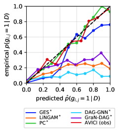
(a)

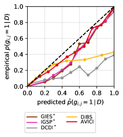
(b)

(a) Linear

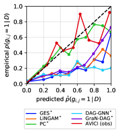
(b)

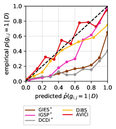
(c)

(b) Rff

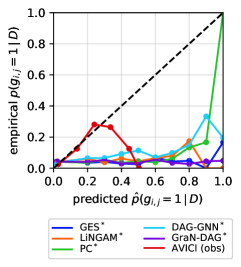
(c)

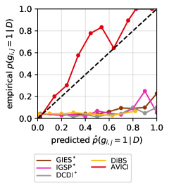
(d)

(c) Grn

Figure 8: Calibration plots ($d=30$) for all methods in the experiments of Section 6.2 and Table 5b. The top and bottom rows of plots show the methods that use observational data and a mix of observational and interventional data, respectively. Methods with an asterix use the nonparametric DAG bootstrap to estimate edge probabilities (Friedman et al., , 1999) (cf. Section 6.2).

Probabilistic metrics

Table 9 summarizes the probabilistic AUROC and AUPRC metrics for all methods in the experiment of Figure 5. Explanations and interpretations for both metrics are given in Section B. The relative performance of the bootstrap baselines and AVICI is similar to the point estimate benchmark. Overall, AVICI performs favorably across the three domains, with GES and GIES on par in Linear. However, since AUROC and AUPRC metrics evaluate the full spectrum of decision thresholds, we additionally see that AVICI achieves nontrivial accuracy in Grn even without access to gene knockout data, indicating that AVICI may provide useful information even in settings where only passive observations are available. This aspect is not apparent when converting the posterior probability estimates of AVICI based on a single threshold and then comparing SID and F1 scores as in Table 1.

Table 9: Probabilistic metrics for the benchmark ($d=30$ variables). Mean AUROC ($\uparrow$) and AUPRC ($\uparrow$) with standard error of all methods on ten random task instances. Methods in the top section use only observational data, in the bottom section both observational and interventional data. We highlight the best result of each section and those within its $95$% confidence interval according to an unequal variances $t$-test.

Linear Rff Grn Algorithm AUROC AUPRC AUROC AUPRC AUROC AUPRC GES^∗ 0.930  (0.01) 0.643  (0.05) 0.759  (0.04) 0.289  (0.06) 0.496  (0.02) 0.045  (0.00) LiNGAM^∗ 0.752  (0.06) 0.365  (0.10) 0.701  (0.04) 0.229  (0.03) 0.537  (0.03) 0.057  (0.01) PC^∗ 0.771  (0.04) 0.469  (0.06) 0.825  (0.04) 0.507  (0.07) 0.510  (0.02) 0.052  (0.01) DAG-GNN^∗ 0.621  (0.03) 0.097  (0.02) 0.693  (0.03) 0.174  (0.01) 0.547  (0.05) 0.082  (0.03) GraN-DAG^∗ 0.685  (0.04) 0.222  (0.03) 0.781  (0.04) 0.419  (0.09) 0.534  (0.08) 0.113  (0.05) AVICI (ours) 0.979  (0.01) 0.767  (0.06) 0.801  (0.07) 0.571  (0.12) 0.678  (0.10) 0.185  (0.04) GIES^∗ 0.981  (0.01) 0.879  (0.04) 0.769  (0.06) 0.389  (0.08) 0.517  (0.03) 0.070  (0.01) IGSP^∗ 0.942  (0.01) 0.660  (0.05) 0.822  (0.04) 0.374  (0.07) 0.471  (0.02) 0.049  (0.01) DCDI^∗ 0.771  (0.03) 0.306  (0.03) 0.740  (0.05) 0.283  (0.06) 0.557  (0.07) 0.113  (0.05) DiBS 0.837  (0.03) 0.524  (0.05) 0.740  (0.05) 0.340  (0.05) 0.517  (0.03) 0.048  (0.01) AVICI (ours) 0.987  (0.01) 0.902  (0.04) 0.862  (0.05) 0.669  (0.10) 0.901  (0.04) 0.656  (0.10) $*$ Nonparametric DAG bootstrap (Friedman et al., , 1999)

References

- Amos, (2022) Amos, B. (2022). Tutorial on amortized optimization for learning to optimize over continuous domains. arXiv preprint arXiv:2202.00665.
- Anderson and Kurtz, (2011) Anderson, D. F. and Kurtz, T. G. (2011). Continuous time markov chain models for chemical reaction networks. In Design and analysis of biomolecular circuits, pages 3–42. Springer.
- Barabási and Albert, (1999) Barabási, A.-L. and Albert, R. (1999). Emergence of scaling in random networks. Science, 286(5439):509–512.
- Barber and Agakov, (2004) Barber, D. and Agakov, F. (2004). The IM algorithm: a variational approach to information maximization. Advances in neural information processing systems, 16(320):201.
- Bassett and Sporns, (2017) Bassett, D. S. and Sporns, O. (2017). Network neuroscience. Nature neuroscience, 20(3):353–364.
- Bennett et al., (2019) Bennett, A., Kallus, N., and Schnabel, T. (2019). Deep generalized method of moments for instrumental variable analysis. Advances in neural information processing systems, 32.
- Bhattacharya et al., (2021) Bhattacharya, R., Nagarajan, T., Malinsky, D., and Shpitser, I. (2021). Differentiable causal discovery under unmeasured confounding. In International Conference on Artificial Intelligence and Statistics, pages 2314–2322. PMLR.
- Bishop and Nasrabadi, (2006) Bishop, C. M. and Nasrabadi, N. M. (2006). Approximate inference. In Pattern recognition and machine learning, volume 4, chapter 10. Springer.
- Blei et al., (2017) Blei, D. M., Kucukelbir, A., and McAuliffe, J. D. (2017). Variational inference: A review for statisticians. Journal of the American statistical Association, 112(518):859–877.
- Bradbury et al., (2018) Bradbury, J., Frostig, R., Hawkins, P., Johnson, M. J., Leary, C., Maclaurin, D., Necula, G., Paszke, A., VanderPlas, J., Wanderman-Milne, S., and Zhang, Q. (2018). JAX: composable transformations of Python+NumPy programs. http://github.com/google/jax.
- Brouillard et al., (2020) Brouillard, P., Lachapelle, S., Lacoste, A., Lacoste-Julien, S., and Drouin, A. (2020). Differentiable causal discovery from interventional data. Advances in Neural Information Processing Systems, 33:21865–21877.
- Buxton, (2009) Buxton, R. B. (2009). Introduction to functional magnetic resonance imaging: principles and techniques. Cambridge university press.
- Chen and Mar, (2018) Chen, S. and Mar, J. C. (2018). Evaluating methods of inferring gene regulatory networks highlights their lack of performance for single cell gene expression data. BMC bioinformatics, 19(1):1–21.
- Chickering, (2003) Chickering, D. M. (2003). Optimal structure identification with greedy search. J. Mach. Learn. Res., 3:507–554.
- Colombo et al., (2014) Colombo, D., Maathuis, M. H., et al. (2014). Order-independent constraint-based causal structure learning. J. Mach. Learn. Res., 15(1):3741–3782.
- Dawid, (2010) Dawid, A. P. (2010). Beware of the DAG! In Proceedings of Workshop on Causality: Objectives and Assessment at NIPS 2008, pages 59–86.
- DeGroot and Fienberg, (1983) DeGroot, M. H. and Fienberg, S. E. (1983). The comparison and evaluation of forecasters. Journal of the Royal Statistical Society: Series D (The Statistician), 32(1-2):12–22.
- Dibaeinia and Sinha, (2020) Dibaeinia, P. and Sinha, S. (2020). Sergio: a single-cell expression simulator guided by gene regulatory networks. Cell Systems, 11(3):252–271.
- Erdős and Rényi, (1959) Erdős, P. and Rényi, A. (1959). On random graphs. Publicationes Mathematicae, 6:290–297.
- Fawcett, (2004) Fawcett, T. (2004). ROC graphs: Notes and practical considerations for researchers. Machine learning, 31(1):1–38.
- Friedman et al., (1999) Friedman, N., Goldszmidt, M., and Wyner, A. (1999). Data analysis with bayesian networks: A bootstrap approach. In Proceedings of the Fifteenth Conference on Uncertainty in Artificial Intelligence, UAI’99, page 196–205, San Francisco, CA, USA. Morgan Kaufmann Publishers Inc.
- Friedman and Koller, (2003) Friedman, N. and Koller, D. (2003). Being Bayesian About Network Structure. A Bayesian Approach to Structure Discovery in Bayesian Networks. Machine Learning, 50(1):95–125.
- Friston et al., (2000) Friston, K. J., Mechelli, A., Turner, R., and Price, C. J. (2000). Nonlinear responses in fmri: the balloon model, volterra kernels, and other hemodynamics. NeuroImage, 12(4):466–477.
- Geiger and Heckerman, (1994) Geiger, D. and Heckerman, D. (1994). Learning gaussian networks. In Proceedings of the Tenth International Conference on Uncertainty in Artificial Intelligence, UAI’94, page 235–243, San Francisco, CA, USA.
- Gilbert, (1961) Gilbert, E. N. (1961). Random plane networks. Journal of the society for industrial and applied mathematics, 9(4):533–543.
- Golub and Van der Vorst, (2000) Golub, G. H. and Van der Vorst, H. A. (2000). Eigenvalue computation in the 20th century. Journal of Computational and Applied Mathematics, 123(1-2):35–65.
- Goudet et al., (2018) Goudet, O., Kalainathan, D., Caillou, P., Guyon, I., Lopez-Paz, D., and Sebag, M. (2018). Causal generative neural networks. arXiv preprint arXiv:1711.08936.
- Guo et al., (2017) Guo, C., Pleiss, G., Sun, Y., and Weinberger, K. Q. (2017). On calibration of modern neural networks. In International conference on machine learning, pages 1321–1330. PMLR.
- Hartford et al., (2017) Hartford, J., Lewis, G., Leyton-Brown, K., and Taddy, M. (2017). Deep IV: A flexible approach for counterfactual prediction. In International Conference on Machine Learning, pages 1414–1423. PMLR.
- Hauser and Bühlmann, (2012) Hauser, A. and Bühlmann, P. (2012). Characterization and greedy learning of interventional markov equivalence classes of directed acyclic graphs. The Journal of Machine Learning Research, 13(1):2409–2464.
- (31) He, K., Zhang, X., Ren, S., and Sun, J. (2015a). Delving deep into rectifiers: Surpassing human-level performance on imagenet classification. In Proceedings of the IEEE international conference on computer vision, pages 1026–1034.
- (32) He, Y., Jia, J., and Yu, B. (2015b). Counting and exploring sizes of markov equivalence classes of directed acyclic graphs. The Journal of Machine Learning Research, 16(1):2589–2609.
- Heckerman et al., (1995) Heckerman, D., Geiger, D., and Chickering, D. M. (1995). Learning Bayesian Networks: The Combination of Knowledge and Statistical Data. Machine Learning, 20(3):197–243.
- Heinze-Deml et al., (2018) Heinze-Deml, C., Maathuis, M. H., and Meinshausen, N. (2018). Causal structure learning. Annual Review of Statistics and Its Application, 5:371–391.
- Hennigan et al., (2020) Hennigan, T., Cai, T., Norman, T., and Babuschkin, I. (2020). Haiku: Sonnet for JAX. http://github.com/deepmind/dm-haiku.
- Hoel et al., (2013) Hoel, E. P., Albantakis, L., and Tononi, G. (2013). Quantifying causal emergence shows that macro can beat micro. Proceedings of the National Academy of Sciences, 110(49):19790–19795.
- Holland et al., (1983) Holland, P. W., Laskey, K. B., and Leinhardt, S. (1983). Stochastic blockmodels: First steps. Social networks, 5(2):109–137.
- Hoyer et al., (2008) Hoyer, P., Janzing, D., Mooij, J. M., Peters, J., and Schölkopf, B. (2008). Nonlinear causal discovery with additive noise models. Advances in neural information processing systems, 21.
- Huynh-Thu and Sanguinetti, (2019) Huynh-Thu, V. A. and Sanguinetti, G. (2019). Gene regulatory network inference: an introductory survey. In Gene Regulatory Networks, pages 1–23. Springer.
- Jin et al., (2020) Jin, C., Netrapalli, P., and Jordan, M. (2020). What is local optimality in nonconvex-nonconcave minimax optimization? In International conference on machine learning, pages 4880–4889. PMLR.
- Kalainathan et al., (2020) Kalainathan, D., Goudet, O., and Dutta, R. (2020). Causal discovery toolbox: Uncovering causal relationships in python. J. Mach. Learn. Res., 21:37–1.
- Kalisch and Bühlman, (2007) Kalisch, M. and Bühlman, P. (2007). Estimating high-dimensional directed acyclic graphs with the pc-algorithm. Journal of Machine Learning Research, 8(3).
- Ke et al., (2022) Ke, N. R., Chiappa, S., Wang, J., Bornschein, J., Weber, T., Goyal, A., Botvinic, M., Mozer, M., and Rezende, D. J. (2022). Learning to induce causal structure. arXiv:2204.04875.
- Kossen et al., (2021) Kossen, J., Band, N., Lyle, C., Gomez, A. N., Rainforth, T., and Gal, Y. (2021). Self-attention between datapoints: Going beyond individual input-output pairs in deep learning. Advances in Neural Information Processing Systems, 34:28742–28756.
- Lachapelle et al., (2020) Lachapelle, S., Brouillard, P., Deleu, T., and Lacoste-Julien, S. (2020). Gradient-based neural dag learning. In International Conference on Learning Representations.
- (46) Lee, H.-C., Danieletto, M., Miotto, R., Cherng, S. T., and Dudley, J. T. (2019a). Scaling structural learning with no-bears to infer causal transcriptome networks. In PACIFIC SYMPOSIUM ON BIOCOMPUTING 2020, pages 391–402. World Scientific.
- (47) Lee, J., Lee, Y., Kim, J., Kosiorek, A., Choi, S., and Teh, Y. W. (2019b). Set transformer: A framework for attention-based permutation-invariant neural networks. In International Conference on Machine Learning, pages 3744–3753. PMLR.
- Li et al., (2020) Li, H., Xiao, Q., and Tian, J. (2020). Supervised whole dag causal discovery. arXiv preprint arXiv:2006.04697.
- Lopez-Paz et al., (2015) Lopez-Paz, D., Muandet, K., Schölkopf, B., and Tolstikhin, I. (2015). Towards a learning theory of cause-effect inference. In International Conference on Machine Learning, pages 1452–1461. PMLR.
- Lorch et al., (2021) Lorch, L., Rothfuss, J., Schölkopf, B., and Krause, A. (2021). DiBS: Differentiable Bayesian structure learning. Advances in Neural Information Processing Systems, 34.
- Louizos et al., (2017) Louizos, C., Shalit, U., Mooij, J. M., Sontag, D., Zemel, R., and Welling, M. (2017). Causal effect inference with deep latent-variable models. Advances in neural information processing systems, 30.
- Löwe et al., (2022) Löwe, S., Madras, D., Zemel, R., and Welling, M. (2022). Amortized causal discovery: Learning to infer causal graphs from time-series data. arXiv preprint arXiv:2006.10833, 140:1–24.
- Marbach et al., (2009) Marbach, D., Schaffter, T., Mattiussi, C., and Floreano, D. (2009). Generating realistic in silico gene networks for performance assessment of reverse engineering methods. Journal of computational biology, 16(2):229–239.
- Mooij et al., (2013) Mooij, J. M., Janzing, D., and Schölkopf, B. (2013). From ordinary differential equations to structural causal models: The deterministic case. In Proceedings of the Twenty-Ninth Conference on Uncertainty in Artificial Intelligence, UAI’13, page 440–448, Arlington, Virginia, USA. AUAI Press.
- Mooij et al., (2020) Mooij, J. M., Magliacane, S., and Claassen, T. (2020). Joint causal inference from multiple contexts. Journal of Machine Learning Research, 21(99):1–108.
- Mooij et al., (2016) Mooij, J. M., Peters, J., Janzing, D., Zscheischler, J., and Schölkopf, B. (2016). Distinguishing cause from effect using observational data: methods and benchmarks. The Journal of Machine Learning Research, 17(1):1103–1204.
- Nandwani et al., (2019) Nandwani, Y., Pathak, A., and Singla, P. (2019). A primal dual formulation for deep learning with constraints. Advances in Neural Information Processing Systems, 32.
- Pascanu et al., (2013) Pascanu, R., Mikolov, T., and Bengio, Y. (2013). On the difficulty of training recurrent neural networks. In International conference on machine learning, pages 1310–1318. PMLR.
- Pearl, (2009) Pearl, J. (2009). Causality. Cambridge university press.
- Peters and Bühlmann, (2014) Peters, J. and Bühlmann, P. (2014). Identifiability of gaussian structural equation models with equal error variances. Biometrika, 101(1):219–228.
- Peters and Bühlmann, (2015) Peters, J. and Bühlmann, P. (2015). Structural intervention distance for evaluating causal graphs. Neural computation, 27(3):771–799.
- Peters et al., (2017) Peters, J., Janzing, D., and Schölkopf, B. (2017). Elements of causal inference: foundations and learning algorithms. The MIT Press.
- Radford et al., (2019) Radford, A., Wu, J., Child, R., Luan, D., Amodei, D., Sutskever, I., et al. (2019). Language models are unsupervised multitask learners. OpenAI blog, 1(8):9.
- Rahimi and Recht, (2007) Rahimi, A. and Recht, B. (2007). Random features for large-scale kernel machines. Advances in neural information processing systems, 20.
- Ravasz et al., (2002) Ravasz, E., Somera, A. L., Mongru, D. A., Oltvai, Z. N., and Barabási, A.-L. (2002). Hierarchical organization of modularity in metabolic networks. science, 297(5586):1551–1555.
- Reisach et al., (2021) Reisach, A. G., Seiler, C., and Weichwald, S. (2021). Beware of the simulated DAG! varsortability in additive noise models. Advances in Neural Information Processing Systems.
- Robinson et al., (2010) Robinson, M. D., McCarthy, D. J., and Smyth, G. K. (2010). edger: a bioconductor package for differential expression analysis of digital gene expression data. Bioinformatics, 26(1):139–140.
- Rubenstein et al., (2017) Rubenstein, P. K., Weichwald, S., Bongers, S., Mooij, J. M., Janzing, D., Grosse-Wentrup, M., and Schölkopf, B. (2017). Causal consistency of structural equation models. In Proceedings of the 33rd Conference on Uncertainty in Artificial Intelligence (UAI), page ID 11.
- Runge et al., (2019) Runge, J., Bathiany, S., Bollt, E., Camps-Valls, G., Coumou, D., Deyle, E., Glymour, C., Kretschmer, M., Mahecha, M. D., Muñoz-Marí, J., et al. (2019). Inferring causation from time series in earth system sciences. Nature communications, 10(1):1–13.
- Sachs et al., (2005) Sachs, K., Perez, O., Pe’er, D., Lauffenburger, D. A., and Nolan, G. P. (2005). Causal protein-signaling networks derived from multiparameter single-cell data. Science, 308(5721):523–529.
- Santoro et al., (2017) Santoro, A., Raposo, D., Barrett, D. G., Malinowski, M., Pascanu, R., Battaglia, P., and Lillicrap, T. (2017). A simple neural network module for relational reasoning. Advances in neural information processing systems, 30.
- Schaffter et al., (2011) Schaffter, T., Marbach, D., and Floreano, D. (2011). Genenetweaver: in silico benchmark generation and performance profiling of network inference methods. Bioinformatics, 27(16):2263–2270.
- Scheines and Ramsey, (2016) Scheines, R. and Ramsey, J. (2016). Measurement error and causal discovery. In CEUR workshop proceedings, volume 1792, page 1. NIH Public Access.
- Schölkopf, (2019) Schölkopf, B. (2019). Causality for machine learning. arXiv preprint arXiv:1911.10500.
- Shalit et al., (2017) Shalit, U., Johansson, F. D., and Sontag, D. (2017). Estimating individual treatment effect: generalization bounds and algorithms. In International Conference on Machine Learning, pages 3076–3085. PMLR.
- Shen-Orr et al., (2002) Shen-Orr, S. S., Milo, R., Mangan, S., and Alon, U. (2002). Network motifs in the transcriptional regulation network of escherichia coli. Nature genetics, 31(1):64–68.
- Shimizu et al., (2006) Shimizu, S., Hoyer, P. O., Hyvärinen, A., Kerminen, A., and Jordan, M. (2006). A linear non-gaussian acyclic model for causal discovery. Journal of Machine Learning Research, 7(10).
- Spirtes et al., (2000) Spirtes, P., Glymour, C. N., and Scheines, R. (2000). Causation, prediction, and search. Adaptive computation and machine learning. MIT Press, Cambridge, Mass, 2nd ed edition.
- Squires et al., (2018) Squires, C., Belyaeva, A., Karnik, S., Saeed, B., Jablonski, K. P., and Uhler, C. (2018). Causaldag. https://github.com/uhlerlab/causaldag.
- Tsamardinos et al., (2006) Tsamardinos, I., Brown, L. E., and Aliferis, C. F. (2006). The max-min hill-climbing Bayesian network structure learning algorithm. Machine learning, 65(1):31–78.
- Vaswani et al., (2017) Vaswani, A., Shazeer, N., Parmar, N., Uszkoreit, J., Jones, L., Gomez, A. N., Kaiser, Ł., and Polosukhin, I. (2017). Attention is all you need. Advances in neural information processing systems, 30.
- Wang et al., (2017) Wang, Y., Solus, L., Yang, K., and Uhler, C. (2017). Permutation-based causal inference algorithms with interventions. Advances in Neural Information Processing Systems, 30.
- Watts and Strogatz, (1998) Watts, D. J. and Strogatz, S. H. (1998). Collective dynamics of ‘small-world’networks. nature, 393(6684):440–442.
- Wilkinson, (2018) Wilkinson, D. J. (2018). Stochastic modelling for systems biology. Chapman and Hall/CRC.
- Yoon et al., (2018) Yoon, J., Jordon, J., and Van Der Schaar, M. (2018). Ganite: Estimation of individualized treatment effects using generative adversarial nets. In International Conference on Learning Representations.
- You et al., (2019) You, Y., Li, J., Reddi, S., Hseu, J., Kumar, S., Bhojanapalli, S., Song, X., Demmel, J., Keutzer, K., and Hsieh, C.-J. (2019). Large batch optimization for deep learning: Training bert in 76 minutes. arXiv preprint arXiv:1904.00962.
- Yu et al., (2019) Yu, Y., Chen, J., Gao, T., and Yu, M. (2019). DAG-GNN: DAG structure learning with graph neural networks. In Proceedings of the 36th International Conference on Machine Learning, volume 97 of Proceedings of Machine Learning Research, pages 7154–7163. PMLR.
- Zhang et al., (2017) Zhang, K., Gong, M., Ramsey, J., Batmanghelich, K., Spirtes, P., and Glymour, C. (2017). Causal discovery in the presence of measurement error: Identifiability conditions. arXiv preprint arXiv:1706.03768.
- Zheng et al., (2018) Zheng, X., Aragam, B., Ravikumar, P. K., and Xing, E. P. (2018). Dags with no tears: Continuous optimization for structure learning. Advances in Neural Information Processing Systems, 31.
- Zhu et al., (2020) Zhu, S., Ng, I., and Chen, Z. (2020). Causal discovery with reinforcement learning. In International Conference on Learning Representations.