Electronic Mach-Zehnder interference in a bipolar hybrid monolayer-bilayer graphene junction

Abstract

Graphene matter in a strong magnetic field, realizing one-dimensional quantum Hall channels, provides a unique platform for studying electron interference. Here, using the Landauer-Büttiker formalism along with the tight-binding model, we investigate the quantum Hall (QH) effects in unipolar and bipolar monolayer-bilayer graphene (MLG-BLG) junctions. We find that a Hall bar made of an armchair MLG-BLG junction in the bipolar regime results in valley-polarized edge-channel interferences and can operate a fully tunable Mach-Zehnder (MZ) interferometer device. Investigation of the bar-width and magnetic-field dependence of the conductance oscillations shows that the MZ interference in such structures can be drastically affected by the type of (zigzag) edge termination of the second layer in the BLG region [composed of vertical dimer or non-dimer atoms]. Our findings reveal that both interfaces exhibit a double set of Aharonov-Bohm interferences, with the one between two oppositely valley-polarized edge channels dominating and causing a large-amplitude conductance oscillation ranging from 0 to $2e^{2}/h$. We explain and analyze our findings by analytically solving the Dirac-Weyl equation for a gated semi-infinite MLG-BLG junction.

I Introduction

Bipolar (n-p) graphene junctions, which form two neighboring regions with different quantum Hall (QH) states, are of tremendous interest for low-dimensional materials because they exhibit unusual and fascinating transport properties Williams2007 ; Abanin2007 ; Huard2007 ; Ozyilmaz2007 . For instance, Abanin et al. Abanin2007 first theoretically addressed QH transport for two regions with different filling factors ($\nu_{1}$ and $\nu_{2}$), predicting new quantized conductance plateaus at values of $G=\frac{|\nu_{1}||\nu_{2}|}{|\nu_{1}|+|\nu_{2}|}\frac{e^{2}}{h}$. This prediction was verified by Williams et al. Williams2007 in experimental transport measurements of the MLG n-p junction. Theoretical studies Tworzydlo2007 ; Myoung2017 ; Trifunovic2019 ; Myoung2020 showed that valley-isospin conservation plays an important role in the evolution of edge states into interface states along the n-p junction of MLG nanoribbons, confirming valley isospin conservation in ribbons with armchair boundaries Tworzydlo2007 ; Trifunovic2019 . Recent experimental studies also show that graphene n-p junction at high magnetic fields hosts (valley- and spin-polarized) edge channels propagating along the junction where coupling between those channels results in a Mach-Zehnder (MZ) interferometer Ji2003 showing Aharonov-Bohm (AB) effect Morikawa2015 ; Wei2017 ; Makk2018 ; Jo2021 .

In addition to bipolar junctions of graphene, hybrid graphene structures consisting of two different areas of graphene layers, e.g., partly monolayer graphene (MLG) and partly bilayer graphene (BLG), also present a lot of interesting physics Puls2009 ; Tian2013 ; Yan2016 ; Zhao2016 ; Du2021 . The Hall resistance across such graphene hybrid structures shows quantized plateaus switching between those of MLG or BLG QH plateaus depending on the type of carriers Tian2013 ; Yan2016 . Experimental study on a dual-gated MLG-BLG junction recently revealed that such graphene channels exhibit different conductance under bias voltage in opposite directions, which also depends on the doping level Du2021 . The energy spectrum of a semi-infinite MLG-BLG junction in the presence of a magnetic field was theoretically studied in Ref. Koshino2010 . The results showed that the valley degeneracy is lifted near the MLG-BLG interface, and oscillatory band structures appear in the boundary region. Such interface states were previously observed as anomalous resistance oscillations in an experimental work by Puls et al Puls2009 . The observation of interface states in a natural junction between MLG and BLG suggests that this graphene system might be used to explore QH edge interface and electron interference in hybrid structures comprising various LL configurations. Electron interferometry is one of the most promising routes for studying coherence effects of electronic states Litvin2007 ; Bieri2009 ; Bocquillon2013 , noise in collision experiments Henny1999 ; Oliver1999 , fractional and non-Abelian statistics Law2006 ; Feldman2006 ; Bid2009 , and quantum entanglement via two particle interference Yurke1992 ; Samuelsson2004 .

Here, we demonstrate that the n-p junction of the MLG-BLG interface bar in a Hall regime results in valley-polarized edge-channel interferences and can operate as an electronic MZ interferometer device. In this paper, using the tight binding model (TBM), we investigate the conductance properties of the MLG-BLG interface for both unipolar and bipolar junctions in the QH regime. We calculate the longitudinal and Hall interface conductances for two types of MLG-BLG interfaces: zigzag 1 [ZZ1, Fig. 1(a)] and zigzag 2 [ZZ2, Fig. 1(b)] using a four-terminal Hall conductor made up of partial MLG and BLG nanoribbons with armchair edges, as shown in Figs. 1(c) and 1(d). ZZ1 is composed of vertical dimer sites ($B1$-$A2$), whereas ZZ2 only has non-dimer $B2$ atoms.

In the case of the unipolar junction, unlike the ZZ2 interface, which exhibits a series of well-realized QH plateaus for longitudinal interface conductance (LIC), the ZZ1 interface shows irregular LIC fluctuations beyond the first QH plateau. In the bipolar regime, both types of MLG-BLG interfaces exhibit a gate tunable Hall interface conductance (HIC) with resonant behavior as a function of Fermi energy. We show that these oscillations result from the AB interference between valley-polarized QH edge channels propagating along the MLG-BLG n-p junction. We analyze our findings by solving the Dirac-Weyl equation analytically and obtaining the energy levels for an ideal n-p junction of semi-infinite MLG-BLG interface. The results show that (three) valley-polarized edge channels (but still spin degenerate) are formed near the MLG-BLG interface, along the n-p junction, and their spatial separations are energy dependent. The spectra of these edge channels differ for ZZ1 and ZZ2 interfaces, resulting in distinct conductance behaviors in each case.

By investigating the bar-width dependence of the conductance oscillations, we demonstrate that as a result of AB interference between those spatially-separated edge channels propagating along the n-p junction, the cross-junction transport shows oscillatory behavior. Our results show a (one-set) regular and a double set of AB oscillations for the ZZ1 and ZZ2 interfaces, respectively. However, in both cases, coupling between two opposite-valley-polarized edge channels is dominant, resulting in a large conductance oscillation with a peak-to-peak amplitude ranging between $0$ and $2e^{2}/h$. On the other hand, studying the magnetoconductances, we see small-amplitude conductance oscillation for both interfaces, which is not noticeable for the ZZ1 boundary and also suppresses as the magnetic field increases; for the ZZ2 boundary, it persists over a wide range of magnetic fields.

The rest of the paper is organized as follows: In Sec. II, we present the proposed structures as well as the basics of our numerical method. Section III is dedicated to results and discussions. In Sec. III.1, we present a comprehensive study of the transport properties of MLG-BLG junction in the unipolar regime and its bipolar junction is investigated in Sec. III.2. Finally, we conclude the manuscript in Sec. IV.

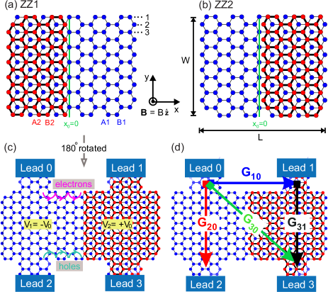
Figure 1: Schematics of a MLG-BLG Hall bar structure (width $W$ and length $L$) with (a) Zigzag 1 (ZZ1) and (b) Zigzag 2 (ZZ2) junctions. (c,d) Four-terminal depiction of the above junctions and the corresponding numbering used to refer to the leads. To describe both ribbons with similar geometry, we rotate panel (a) by $180^{\circ}$ to obtain panel (c). The purple and cyan snake-like curves in panel (c), respectively, indicate the electron and hole edge state chiralities for the given direction of the magnetic field, $\hat{\mathbf{z}}$ axis. Bipolar MLG-BLG junction is created by applying the potentials $V_{1}=-V_{0}$ and $V_{2}=V_{0}$ to the MLG and BLG parts, respectively. The longitudinal conductance $G_{10}$ (blue) and Hall conductances of the MLG part $G_{20}$ (red), BLG part $G_{31}$ (black), and MLG-BLG interface $G_{30}$ (green) are shown in panel (d) with the corresponding colors which we use to indicate them in the numerical plots.

II Theory and model

We consider a bipolar quantum Hall graphene bar consisting of MLG-BLG junction as shown in Fig. 1. Geometrically, this structure can be regarded as a (AB-stacked) BLG ribbon in which half of its upper layer is cut out, thus creating the MLG-BLG junction. We assume that the lower layer of BLG part, containing $A1$ and $B1$ sublattices, seamlessly continues to the MLG part with A and B sublattices, while the upper graphene layer composed of $A2$ and $B2$ sublattices is sharply terminated at the boundary. Depending on which part of the upper layer in BLG ribbon is removed, one would have two distinct boundaries labeled as ZZ1 and ZZ2. In the case of ZZ1 termination [Fig. 1(a)], the outermost atoms of the upper layer are $A2$ atoms that directly couple to the $B1$ atoms of the lower layer (dimer atoms), whereas in the case of ZZ2 termination, the $B2$ atoms on the upper layer [having no counterpart from the lower layer (non-dimer atoms)] form the front-most line of the bilayer region [Fig. 1(b)]. Furthermore, we use metallic armchair ribbon, the width of which is characterized by $N=3m-1$ ($m$ being an integer), referring to the number of horizontal dimer lines of the ribbon as illustrated in Fig. 1(a).

Using a single-orbital TBM for $p_{z}$ atomic orbital of carbon, which in a second quantization formalism can be written as

$$\mathcal{H}=\sum_{i}(\epsilon_{i}+V_{i})c^{\dagger}_{i}c_{i}-\sum_{\langle i,j\rangle}t_{ij}c^{\dagger}_{i}c_{j}+\text{H.c.},$$ (1)

where $c^{\dagger}_{i}$ and $c_{i}$ are, respectively, the creation and annihilation operators for an electron on the $i$th lattice site with on-site energy $\epsilon_{i}$ and $V(x)=V_{0}\tanh(x/\xi)$ is a position-dependent potential applied to the structure. As shown in Fig. 1(c), $V(x)$ takes the values of $-V_{0}$ and $+V_{0}$ in the MLG ($x<0$) and BLG ($x>0$) regions, respectively, thus separating n-doped region for $x<0$ from p-doped region for $x>0$. Notice that $\xi\rightarrow 0$ introduces an abrupt step n-p junction, while $\xi\neq 0$ indicates a smoothly varying potential. In this paper, we used $\xi=0.05$ nm representing the first case. In the second term of Hamiltonian (1), $t_{ij}$ is the hopping transfer integral between two atoms ($i$, $j$) and $\langle i,j\rangle$ denotes a summation over nearest neighbor sites. Here, we use a simple model for MLG and BLG, with only $\gamma_{0}=-2.7$ eV and $\gamma_{1}=0.48$ eV describing the nearest-neighbor intralayer and interlayer hopping $t_{ij}$, respectively.

The effect of a perpendicular magnetic field ($\mathbf{B}=B\,\hat{\mathbf{z}}$) can be introduced into the calculations via the Peierls substitution Peierls1933 $t_{ij}\rightarrow t_{ij}\mathrm{e}^{\mathrm{i}\,2\pi\Phi_{ij}}$ where $\Phi_{ij}=(1/\Phi_{0})\int^{\mathbf{r}_{j}}_{\mathbf{r}_{i}}\mathbf{A}(\mathbf{r})\cdot d\mathbf{r}$ is the Peierls phase with $\Phi_{0}=h/e\approx 4.14\times 10^{-15}\ \mathrm{T.m^{2}}$ the magnetic flux quantum and $\mathbf{A}(\mathbf{r})=(0,Bx,0)$ the vector potential in the Landau gauge for which $\Phi_{ij}$ is given by $\Phi_{ij}=(y_{j}-y_{i})(x_{j}+x_{i})B/2\Phi_{0}$.

In the linear response regime, the Landauer-Büttiker formalism provides a rigorous formalism to describe multi-terminal conductance measurements in Hall bars as Datta1997

$$G_{pq}(E)=\frac{2e^{2}}{h}\sum_{m\in q}\sum_{n\in p}|s_{nm}|^{2}\,.$$ (2)

Here, $G_{pq}(E)$ represents the conductance from lead (or terminal) $q$ to lead $p$ at the energy $E$ and $s_{nm}$ is the scattering matrix ($S$-matrix) from mode $m$ in lead $q$ to mode $n$ in lead $p$. In order to investigate the conductance of the four-terminal Hall bar [Figs. 1(c,d)], we use the Kwant package Kwant2014 , which employs $S$-matrix formalism in conjunction with the TBM to calculate quantum transport properties of materials.

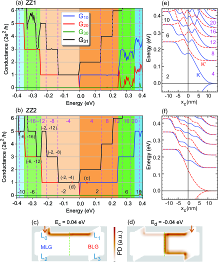
Figure 2: Four-terminal conductance of a unipolar MLG-BLG quantum Hall bar as a function of the Fermi energy for (a) ZZ1 and (b) ZZ2 interfaces at the magnetic field of $B=60$ T. The results are shown for a metallic armchair graphene ribbon with $L=169.87$ nm and $W=51.91$ nm. Colored regions represent different bulk filling factors of MLG with the corresponding numbers shown in the lower part of panel (b) as $\nu_{1}=\pm 2,\pm 6,\pm 10$. The corresponding filling factors of BLG, $\nu_{2}=\pm 4,\pm 8,\pm 12$, are represented by the purple numbers in the upper side of the panel (b) between the vertical dashed purple lines. (c, d) Probability densities (PD) corresponding to the energies marked by (c) and (d) in panel (b) at the Fermi energies $E_{c}=0.04$ and $E_{d}=-0.04$, respectively. In panels (c) and (d), the propagating modes enter from lead 0 and 1, respectively. (e, f) Energy spectrum of a half-infinite MLG-BLG junction versus the center of the cyclotron orbit $x_{c}=-k_{y}l_{B}^{2}$ obtained by solving the Dirac-Weyl equation analytically (Appendix) with (e) ZZ1 and (f) ZZ2 interfaces. Blue solid (red dashed) curves refer to the $K$ ($K^{\prime}$) valley. As seen, the energy levels approach the bulk Landau quantization of MLG and BLG in the left and right side of the spectrum, respectively.

III Results and discussion

III.1 Unipolar MLG-BLG quantum Hall bar

We first consider the unipolar and bipolar MLG-BLG Hall bar with both ZZ1 and ZZ2 monolayer-bilayer interfaces as illustrated in Figs. 1(a) and 1(b), respectively. In the proposed four-terminal hybrid Hall bar [Figs. 1(c) and 1(d)], we measure the LIC $G_{10}$, Hall conductances of the MLG part $G_{20}$, BLG part $G_{31}$, and MLG-BLG interface $G_{30}$, simultaneously. Using these conductances enables us to individually measure the splitting of the conductance at the interface of the hybrid structure. In this paper, we present the results for a metallic armchair graphene ribbon with $L=169.87$ nm and $W=51.91$ nm that is subjected to a perpendicular magnetic field of $B=60$ T for which the corresponding magnetic length is $l_{B}=\sqrt{\hbar/eB}=3.31$ nm. We use a rather strong $B$ here to ensure $l_{B}\ll W$ as well as leads width, $l_{B}<l_{w}\approx 25.50$ nm. It is worth to mentioning that, for the study of the electronic properties of graphene nanostructures in the presence of a perpendicular magnetic field, one can define a scaling factor and thus extend the results to lower magnetic field and larger sampsle sizes, e.g., see Refs. Makk2018 ; Liu2015 ; Cabosart2017 . Furthermore, for the given magnetic field direction, $\hat{\mathbf{z}}$ axis, the corresponding edge state chiralities for electrons and holes are clockwise (CW) and anticlockwise (ACW), respectively [see Fig. 1(c)].

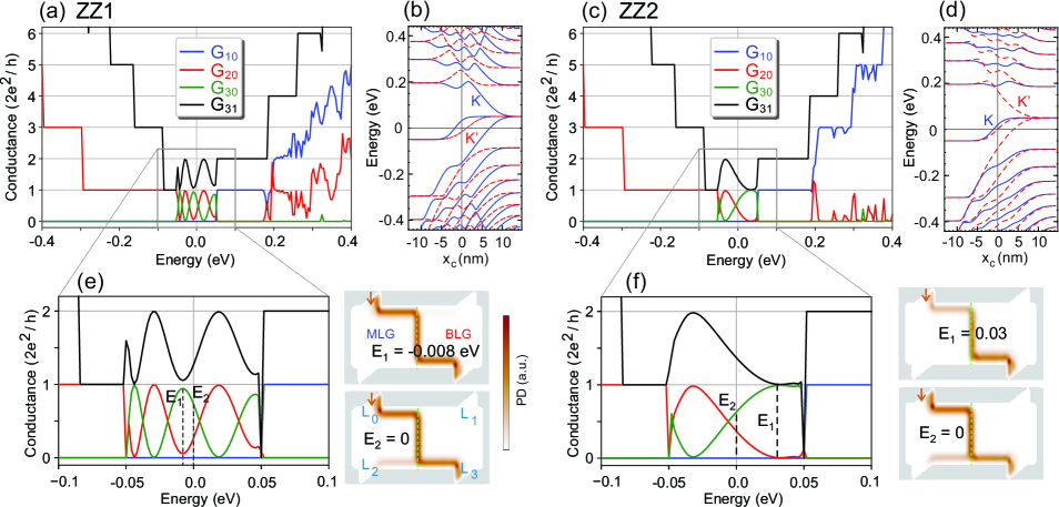
Figure 3: (a,c) Four-terminal conductance of a bipolar MLG-BLG quantum Hall bar as a function of Fermi energy for (a) ZZ1 and (c) ZZ2 interfaces. The applied potentials to the MLG and BLG parts, respectively, are $V_{1}=-V_{0}$ and $V_{2}=V_{0}$ with $V_{0}=0.05$ eV. (b,d) Energy spectrum of the half-infinite MLG-BLG n-p junction versus the center of the cyclotron orbit $x_{c}=-k_{y}l_{B}^{2}$ obtained analytically for (b) ZZ1 and (d) ZZ2 interfaces. Blue solid (red dashed) curves refer to the $K$ ($K^{\prime}$) valley. (e,f) Enlarged views of the conductances around the bipolar energy range, as indicated by grey boxes in (a) and (c) panels. The rightmost figures in each panel show the probability densities (PD) of the propagating modes coming in from lead 0 for each interface at the two different Fermi energies $E_{1}$, $E_{2}$, which are labeled in panels (e) and (f).

We begin by analyzing the measured conductances $G_{10}$, $G_{20}$, $G_{30}$, and $G_{31}$ for a unipolar MLG-BLG junction. Figures 2(a) and 2(b) show the conductances as a function of Fermi energy for (a) ZZ1 and (b) ZZ2 MLG-BLG interfaces in the unipolar junction. For both interfaces, we see that the $G_{20}$ (red curve) exhibits the standard MLG QH plateaus (odd numbers of $2e^{2}/h$) for hole states ($E<0$) with the ACW chirality and the $G_{31}$ (black curve) in the BLG part shows the BLG QH plateaus (even numbers of $2e^{2}/h$) for electron states ($E>0$) with the CW chirality. The conductance quantization represented by $G_{31}$ for the hole states ($E<0$) and $G_{10}$ (LIC) for $E>0$ in both ribbons can be explained by the theory addressed in Refs. Williams2007 ; Abanin2007 . According to this model, in a unipolar regime n-n or p-p, the conductance values across the interface (e.g., $G_{10}$) follow

$$G=\mathrm{min}(|\nu_{1}|,|\nu_{2}|)\times\frac{e^{2}}{h},$$ (3)

where $\nu_{1}$ ($=\pm 2,\ \pm 6,\ \ldots$) and $\nu_{2}$ ($=\pm 4,\ \pm 8,\ \ldots$) are the filling factors in the MLG and BLG regions, respectively. As a result, the remaining edge modes $|\nu_{1}-\nu_{2}|$ in the region of maximum absolute filling factor propagate along the interface and return back to that region. For example, in Fig. 2(b), each stepwise value of $G_{31}$ for hole states can be obtained by applying this analysis with the corresponding filling factors $(\nu_{1},\ \nu_{2})$ defined at each conductance plateau depending on the Fermi energy, as depicted in Fig. 2(b). Here, the colored regions represent different bulk filling factors of MLG as $\nu_{1}=\pm 2,\pm 6,\pm 10$ and the regions between the vertical dashed purple lines refer to the corresponding filling factors of BLG, i.e., $\nu_{2}=\pm 4,\pm 8,\pm 12,\pm 16$. Notice that the LLs of MLG and gapless BLG can be obtained using $E_{n}^{M}=\pm v_{F}\sqrt{2e\hbar nB}$ and $E_{n}^{B}=\pm\sqrt{n(n-1)}\hbar eB/m^{*}$ ($n=0,1,2,\ldots$), respectively, with $m^{*}=\gamma_{1}/2v_{F}^{2}$ representing the effective mass of quasiparticles Novoselov2005 ; Rutter2011 . Further, for both ribbons, there is no HIC $G_{30}$ measured between leads 0 and 3 as shown by green curves in Figs. 2(a) and 2(b).

The above discussion can be highlighted further by plotting the probability densities for the two representative Fermi energies denoted by (c) and (d) in Fig. 2(b). For the electron Fermi energy (c) [see Fig. 2(c)], one can see that the coming modes from lead 0 completely pass the interface along the edge of the Hall bar, resulting in $G_{10}=2e^{2}/h$. In state (d), modes from lead 1 in the BLG region split up at the interface, are partially transmitted across the interface, and the remaining modes propagate through the interface and return to the BLG region [Fig. 2(d)].

Beyond the first MLG filling factor area, however, the longitudinal conductance $G_{10}$ (blue curve) and the Hall one $G_{31}$ (black curve) exhibit different behaviors for ZZ1 and ZZ2 interfaces. For the ZZ2 interface, $G_{10}$ and $G_{31}$ exhibit well-realized QH plateaus, whereas the ZZ1 interface exhibits irregular conductance fluctuations, cf. Figs 2(a) and 2(b). This can be attributed to the different behavior interface states that appear near the boundary region. Analytically, we solve the Dirac-Weyl equation for a composed system of a half-infinite graphene monolayer and bilayer, similar to the structure studied in Ref. Koshino2010 (see also the Appendix), and plot the energy levels as a function of the cyclotron orbit center $x_{c}=-k_{y}l_{B}^{2}$ ($l_{B}$ is the magnetic length), as shown in Figs. 2(e) and 2(f). As seen, the interface LLs for the ZZ2 interface exhibit monotonic dependence, whereas it is nonmonotonic in the ZZ1, indicating that the energy coupling between the MLG and BLG regions is weaker in the ZZ1 interface than in the ZZ2 interface, as also discussed in Ref. Koshino2010 . Except for the fine differences reported here between the two ZZ1 and ZZ2 interfaces, our numerical results are consistent with the experimental results reported in Refs. Tian2013 ; Yan2016 for unipolar hybrid MLG-BLG structures. Because realistic structures will have irregular and mixed edge types, flawless edge terminations are required to observe such differences.

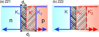
Figure 4: Schematic of edge-channel configurations and principle of AB interference between the edge states propagating along the n-p junction for (a) ZZ1 and (b) ZZ2 interfaces. The solid blue ($K$) and dashed red ($K^{\prime}$) lines depict three valley-polarized edge channels for each interface, as predicted by the analytical results [Figs. 3(b) and 3(d)]. $d_{s}$ ($d_{l}$) shows the spatial distance between two neighboring (far-distant) edge channels, and the enclosed area defined by those channels is indicated by the left-angle-hatched (right-angle-hatched) area.

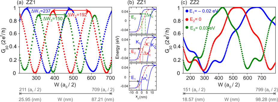
Figure 5: The Hall interface conductance $G_{30}$ of a bipolar MLG-BLG junction as a function of ribbon width for (a) ZZ1 and (b) ZZ2 interfaces ($V_{1}=-V_{2}=-0.05$ eV). The results are presented for three selected Fermi energies $E_{1}=-0.02$ eV (blue), $E_{2}=0$ (red), and $E_{3}=0.03$ eV (green). Panel (b) is a zoom-in plot of the analytical energy levels of the ZZ1 interface [shown in Fig. 3(b)] around the bipolar energy window. In each plot, we show the spatial distance $\Delta x^{i}_{c}$ ($i=1,2,3$) between the two neighboring edge channels $K_{1}$ and $K^{\prime}$ corresponding to the energy states $E_{i}$.

III.2 Bipolar MLG-BLG quantum Hall bar

The character of quantum Hall edge transport in the n-p junction is quite different. In Fig. 3, we plot the conductances for the same Hall bars as in the previous section, by applying the potentials $V_{1}=-V_{0}$ and $V_{2}=V_{0}$ ($V_{0}=0.05$ eV) to the MLG and BLG regions, respectively. In this case, either side of the junction gives electron- and hole-like edge modes with opposite edge chiralities and results in metallic channels at the interface Abanin2007 ; Williams2007 . Accordingly, as seen in Figs. 3(e) and 3(f), the LIC within the bipolar energy $|E|<V_{0}$ is $G_{10}=0$, whereas the Hall conductances $G_{20}$ and $G_{30}$ become nonzero and exhibit oscillatory behavior due to the presence of the interface channel. Below, we discuss and show that these oscillations result from the interference between two parallel edge states that belong to two different valleys. Note that the conductances for the ZZ1 and ZZ2 interfaces exhibit different profiles. As seen, the Hall bar with ZZ1 interface exhibits more oscillatory behavior within the bipolar regime. Further, in this regime, $G_{20}$, $G_{30}$ and $G_{31}$, $G_{30}$, respectively, satisfy the sum rules $G_{20}+G_{30}=2e^{2}/h$ and $G_{31}+G_{30}=4e^{2}/h$, reflecting the conservation of Hall edge modes in the MLG and BLG parts, respectively. Therefore, only the HIC conductance $G_{30}$ is discussed hereafter.

To further characterize the transport fingerprints of the interface channels, we plot, in Figs. 3(b) and 3(d), the analytical energy levels of the MLG-BlG n-p junction as a function of $x_{c}$ for the two interfaces, ZZ1 and ZZ2, respectively. As seen, there are three edge channels near the MLG-BLG junction. In both interfaces, two edge states belonging to two different valleys $K$ and $K^{\prime}$, and originating from zero electron and hole LLs are formed near the MLG-BLG junction (neighboring edge states), while the third one is formed rather far away from the physical MLG-BLG boundary. For the ZZ1 and ZZ2 interfaces, we will refer to them as ($K_{1},K^{\prime},K_{2}$) and ($K,K^{\prime}_{1},K^{\prime}_{2}$), respectively, starting from the left side in Figs. 3(b) and 3(d). Notice that these edge states are still spin degenerate. Due to the interference between the spatially-separated edge states propagating along the n-p junction, the cross-junction transport shows an oscillatory behavior. The coupling between the edge channels propagating along the n-p junction is illustrated schematically in Fig. 4. Two copropagating QH edge states encircle an enclosed area $S$ ($=Wd$), and thus, under the perpendicular magnetic field $B$, they acquire a phase difference $\Phi=BS$ arising from the AB effect. The conductance oscillations can be described phenomenologically by Wei2017 ; Jo2021

$$G(E)\propto\cos(2\pi\frac{\Phi}{\Phi_{0}}+\varphi_{0}),$$ (4)

where $\varphi_{0}$ generally is an unknown phase associated with other effects. However, here, because of our well-defined armchair-edged ribbons, it corresponds to the angle between the valley isospins at the two edges of the nanoribbon Tworzydlo2007 . We argue and provide details below that the observed oscillations for the studied structures result from the AB interference between the QH edge states near the MLG-BLG n-p junction.

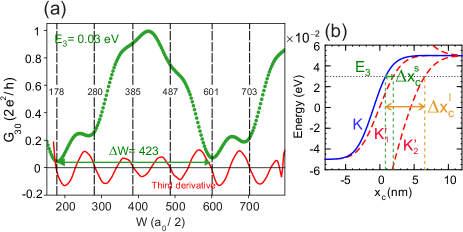
Figure 6: (a) The Hall interface conductance $G_{30}$ (green) and its third numerical derivative (red) as a function of ribbon width for the ZZ2 interface at $E_{3}=0.03$ eV. Vertical dashed lines with the integer values of $W(a_{0}/2)$ indicate the successive (local) minima positions. (b) Zoom-in plot of the analytical energy levels of the ZZ1 interface [shown in Fig. 3(d)] around the bipolar energy window. Vertical green (orange) dashed lines show the $\Delta x_{c}^{s}$ ($\Delta x_{c}^{l}$) as the distance between the two edge channels $K$ and $K^{\prime}_{1}$ ($K$ and $K^{\prime}_{2}$) at $E_{3}=0.03$ eV.

Figure 5 shows the HIC conductance as a function of the Hall bar width for both interfaces (a) ZZ1 and (c) ZZ2. Here, we vary the width of the ribbons so that both remain metallic. The results are presented for three representative Fermi energies in the bipolar regime, e.g., $E_{1}=-0.02$ eV, $E_{2}=0$, and $E_{3}=0.03$ eV at $B=60$ T. In the case of the ZZ1 interface, shown in Fig. 5(a), we see regular conductance oscillations with different periods for each Fermi energy as $W$ varies. This implies that the variation of the AB phase $\Phi=Bd\Delta W$ only comes from $\Delta W$, and that the spatial distance between the edge states ($d$) along the n-p junction is constant for each energy state. From the AB phase, for a period of conductance oscillation in Fig. 5(a), we obtain the spatial separation of the two edge channels

$$d=\frac{\Phi_{0}}{B\Delta W}$$ (5)

for each energy state as $d_{1}\approx 2.36$ nm, $d_{2}\approx 2.92$ nm, and $d_{3}\approx 3.74$ nm. Using the analytical energy spectrum [Fig. 5(b)], we also find $\Delta x_{c}^{1}\approx 2.34$ nm, $\Delta x_{c}^{2}\approx 2.93$ nm, and $\Delta x_{c}^{3}\approx 3.70$ nm as the analytical splitting between the two neighboring edge channels $K_{1}$ and $K^{\prime}$, for the energy states $E_{1}$, $E_{2}$, and $E_{3}$, respectively. Surprisingly, we find a strong agreement between the two results.

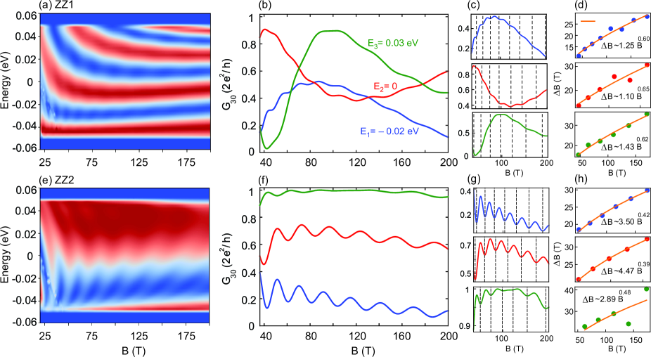
Figure 7: (Upper panels) (a) 2D color plot of the Hall conductance $G_{30}$ of an n-p MLG-BLG junction as functions of energy and magnetic field $B$ for ZZ1 interface. (b) $G_{30}$ as a function of magnetic field for three selected energy states $E_{1}=-0.02$ eV (blue), $E_{2}=0$ (red), and $E_{3}=0.03$ eV (green). Plots in (c) show the conductances separately for each energy state, with vertical dashed lines indicating successive minima positions. (d) Corresponding magnetic field spacing ($\Delta B$) between the successive minima extracted from panel (c). In each case, the fitting (orange curve) appears to show a $\sim B^{1/2}$ dependence of $\Delta B$ as a function of magnetic field. (Lower panels) The same as the upper panels, but for the ZZ2 interface.

Conductance behaves differently in the case of the ZZ2 interface. Whereas conductance for the ZZ1 interface shows only one set of oscillations, the ZZ2 interface shows two sets. A double set of oscillations may indicate the presence of two distinct AB interference loops operating near the n-p junction. We attribute the small oscillations to the AB interference between the $K$ and $K^{\prime}_{2}$ edge channels and the large ones to the AB interference between the two neighboring edge states, i.e., $K$ and $K^{\prime}_{1}$ [see Fig. 6(b)]. To support our statement quantitatively, the conductance corresponding to the energy state of, e.g., $E_{3}=0.03$ eV and its numerical third derivative as a function of $W$ are shown in Fig. 6(a). Using the Eq. (5), we find (averaged) $d^{\mathrm{l}}=5.35$ nm for small $\Delta W$ periods, which are represented by vertical dashed lines in Fig. 6(a). The corresponding spatial distance between the $K$ and $K^{\prime}_{2}$ edge states, extracted from the analytical results [shown in orange in Fig. 6(b)], is $\Delta x_{c}^{\mathrm{l}}=5.47$ nm, which agrees very well with the $d^{l}$ obtained from the AB-interference description. Using Eq. (5) with $\Delta W=423\,a_{0}/2$ between two minima of the large oscillation [Fig. 6(a)], we obtain $d^{\mathrm{s}}=1.32$ nm, which agrees well with $\Delta x_{c}^{\mathrm{s}}=1.29$ nm extracted from the analytical results for the two neighboring edge states ($K$, $K^{\prime}_{1}$) at the corresponding energy state $E_{3}=0.03$ eV, as shown by the green arrow in Fig. 6(b). The two measurements are perfectly consistent and confirm our interpretation.

Notice that in both interfaces, conductance oscillation amplitude $\Delta G_{03}$ as a result of coupling between the two adjoining edge channels (belonging to distinct valleys), varies approximately between 0 and $2e^{2}/h$. $\Delta G_{03}$ variation owing to the coupling between two far-distant edge channels, on the other hand, is not noticeable in the case of the ZZ2 interface and is nearly absent in the ZZ1 interface. This indicates that the AB interference between the two edge channels with opposite valleys and spatially adjacent to each other is significant and mostly mediates the transport across the junction.

Probability densities corresponding to examples of energies, as labeled by $E_{1,2}$ in Figs. 3(e) and 3(f), are shown at the right of each panel. A (valley-degenerate) edge channel coming from lead 0 in the MLG region is wholly guided along the n-p junction at the intersection between the ribbon physical edge and the n-p interface, and splits into valley-polarized channels due to the presence of the second layer of BLG region, which, after traveling along the n-p junction, obtain different AB phases, interfere at the bottom ribbon physical edge and result in two complementary edge channels, collected by leads 1 and 2. As can be seen, the outcome leads to full ($E_{1}$ in each panel) or finite ($E_{2}$) transmission, depending on the Fermi energy. This mechanism is the electronic analogue of the optical MZ interferometer, which was first introduced by Ji et al. Ji2003 .

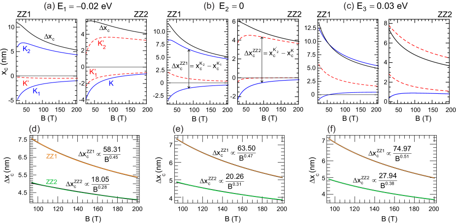
Figure 8: The cyclotron orbit position $x_{c}$ of the three edge channels formed in the bipolar regime [Figs 3(b) and 3(d)] as a function of the magnetic field for three examples of the energy states (a) $E_{1}=-0.02$ eV, (b) $E_{2}=0$, and (c) $E_{3}=0.03$ eV. In each case, the left (right) panel shows the result for ZZ1 (ZZ2) interface. Blue solid (red dashed) curves refer to the $K$ ($K^{\prime}$) valley. Black curves depict the difference between the two far-distant edge channels which is defined as $\Delta x_{c}^{ZZ1}=|x_{c}^{K_{2}}-x_{c}^{K_{1}}|$ and $\Delta x_{c}^{ZZ2}=|x_{c}^{K^{\prime}_{2}}-x_{c}^{K}|$ for the ZZ1 and ZZ2 intefaces, respectively. The lower panels show the power-law dependence $\sim\alpha B^{\beta}$ of the $\Delta x_{c}$ for the ZZ1 (orange) and ZZ2 (green) interfaces corresponding to the upper panels’ energies (d) $E_{1}$, (e) $E_{2}$, and (f) $E_{3}$.

Now, we analyze the magnetic-field dependence of the HIC conductance for both interfaces. Figures 7(a) and 7(e) show a two-dimensional (2D) color plot of HIC as a function of magnetic field in the bipolar energy window for both interfaces ZZ1 and ZZ2, respectively. One can obviously see two different conductance profiles for two boundaries. While the conductance as a function of energy in the ZZ1 interface becomes more oscillatory as $B$ increases, the ZZ2 interface exhibits low and high conductances for low and high energies, respectively. In the following, we show that the $B$-dependency of the HIC in both cases supports the AB oscillations idea for the considered MLG-BLG interfaces.

Figures 7(b) and 7(f) show the magnetoconductance at three selective Fermi energies $E_{1}=-0.02$ eV, $E_{2}=0$, and $E_{3}=0.03$ eV for the ZZ1 and ZZ2 interfaces, respectively. The magnetoconductance oscillations are reminiscent of the AB oscillation. Here also notice that a double set of oscillations can be considered for both interfaces. Small oscillations (due to AB interference between two distant edge channels), as seen in Figs. 7(b) and 7(f), and large oscillations (due to coupling between two neighboring edge channels), whose periodicities are not covered in the shown $B$-range. For both interfaces, in the case of small oscillations, all three conductances reveal a different period of $\Delta B$, as expected. Because, as previously stated, the spatial separation ($d$) of the edge channels varies depending on the energy state. According to the relation $\Delta B(Wd)=\Phi_{0}$, one expects a constant $\Delta B$ for a fixed edge-channel separation $d$ at each energy state. However, magnetoconductances exhibit a common trend, namely the increase of $\Delta B$ with increasing of $B$ [Figs. 7(c,d,g,h)]. The magnetic-field spacing ($\Delta B$) derived from the successive maxima (or minima) of the magnetoconductance curves is separately shown for each energy state in Figs. 7(d) and 7(h) for both interfaces. It seems that both interfaces share a common trend $\sim B^{1/2}$. Our calculations for a wide range of $B$ fields, such as $40-500$ T (not shown here), show this dependency with high precision, i.e., $\Delta B\propto B^{0.50}$ and consequently the spatial separation of the edge channels decreases by $d\propto 1/B^{1/2}$. This behavior is in contrast with that of an MLG n-p junction for which the magnetoconductance oscillations in the QH regime reveal a linear decrease of $\Delta B$ as a function of $B$ Morikawa2015 ; Makk2018 .

It is also worth noting that the (small) oscillation amplitude for the ZZ1 boundary is not remarkable and vanishes as the magnetic field increases; for the ZZ2 boundary, it persists for the entire magnetic-field range, indicating that coupling between two far-distant edge channels in the ZZ1 boundary is weaker than that of the ZZ2 boundary which is consistent with what we discussed in Figs. 5(a) and 5(c) where the ZZ2 boundary shows a double set of AB interference. This can be understood as follows. As shown in Fig. 4, the two rightmost edge channels of the ZZ1 boundary are from two different valleys ($K^{\prime},K_{2}$), whereas the two rightmost edge channels of the ZZ2 boundary are from the same valley ($K^{\prime}_{1},K^{\prime}_{2}$). As a result, any interchannel scattering from the leftmost edge channel (belonging to $K$ valley in both cases) to the rightmost channel in the case of ZZ1 interface requires two intervalley scattering process $K\rightarrow K^{\prime}\rightarrow K$ costing more energy than the ZZ2 case, which requires only one scattering process $K\rightarrow K^{\prime}$.

The above-predicted $B$-dependence of the spatial separation of the edge channels, i.e., $d\propto 1/B^{1/2}$, is consistent with our analytical results. Figure 8 depicts the cyclotron orbit position $x_{c}$ of the (three) interface edge channels [Figs 3(b) and 3(d)] as a function of the magnetic field for the studied selective energies (a) $E_{1}=-0.02$ eV, (b) $E_{2}=0$, and (c) $E_{3}=0.03$ eV. In each case, the results are presented for both interfaces, ZZ1 (left panel) and ZZ2 (right panel). We also plot the $\Delta x_{c}$ (black curves) for the two far-distant edge channels defined in the ZZ1 and ZZ2 plots shown in Fig. 8(b). As seen, in both cases, the spatial separation of the edge channels decreases as the $B$ field increases. By fitting the $\Delta x_{c}$ to the power low $\alpha/B^{\beta}$ [lower panels in Fig. 8], we obtain a $\sim 1/B^{0.50}$ and $\sim 1/B^{0.30}$ dependence for the edge-channel separations in the case of ZZ1 and ZZ2 interfaces, respectively. This is in agreement with what was predicted in the magnetoconductance oscillations shown in Figs. 7(d) and 7(h).

Figure 9: The Hall interface conductance $G_{30}$ of a bipolar MLG-BLG junction as a function of the n-p-junction position $x_{np}$ at Fermi energy $E=0$ for ZZ1 (blue) and ZZ2 (orange) interfaces when the applied potential is (a) abrupt ($\xi=0.05$ nm) and (b) smoothly varying ($\xi=5$ nm).

To complement our analysis, we perform the transport calculations for the structures when the n-p-junction position does not coincide with the physical MLG-BLG interface at $x_{0}=0$. Figure 9(a) shows the HIC of a bipolar MLG-BLG junction as a function of the n-p-junction position, $x_{np}$, at Fermi energy $E=0$ for both interfaces. The results are presented in steps of $a_{cc}=0.142$ nm (C-C distance) from $x_{np}=-72a_{cc}\approx-10.23$ nm in the MLG region to $x_{np}=150a_{cc}\approx 21.30$ nm in the BLG region. The small rapid oscillations in Fig. 9(a) are caused by an abrupt step potential ($\xi=0.05$ nm), which does not exist with a smoothly varying potential ($\xi=5$ nm), as shown in Fig. 9(b). We see that when the n-p junction ($x_{np}$) is tuned in the MLG region far away from the MLG-BLG interface, the conductance shows a plateau at $2e^{2}/h$ for both interfaces, which is consistent with previous study in Ref. Tworzydlo2007 . This result is also consistent with our analytical calculations, which show that in the case of the MLG n-p junction, the formation of an edge channel in the bipolar energy is not valley polarized; see Fig. A1(a) in the appendix. As a result, there is no AB interference between the two degenerate edge channels propagating along the n-p interface, resulting in a conductance plateau at $2e^{2}/h$ Tworzydlo2007 . However, as previously stated, valley- and spin-polarized edge channels in a graphene n-p junction can be created experimentally, allowing for the realization of a MZ interferometer in such structures Morikawa2015 ; Wei2017 ; Makk2018 ; Jo2021 .

Approaching the $x_{np}$ to the physical MLG-BLG interface, where the valley degeneracy is lifted for both interfaces, influences the HIC as a result of the AB interference. Notice that the two interfaces exhibit different profiles. While the ZZ1 interface exhibits full transmissions or full back-reflections depending on the exact position of the $x_{np}$ in the MLG region, the ZZ2 interface exhibits a finite transmission that approaches zero as the $x_{np}$ approaches to the MLG-BLG junction. This property is shared by all energies in the bipolar regime. Shallow oscillations persist in the BLG region in consistent with our analytical calculations, which show two (valley-degenerate) edge channels along the n-p junction of a gated BLG structure in the bipolar regime [see Fig. A1(b)].

IV Conclusion

In conclusion, we demonstrated that an n-p junction of MLG-BLG interface bar in the Hall regime results in valley-polarized edge-channel interferences and can function as a fully tunable MZ interferometer device. Using the Landauer-Büttiker formalism along with the TBM, we investigated the conductance properties of unipolar and bipolar hybrid MLG-BLG junctions in two different interfaces known as ZZ1 and ZZ2 boundaries. Our findings show that, in contrast to the ZZ2 interface, the ZZ1 interface affects the higher QH plateaus in a unipolar MLG-BLG junction, indicating that the coupling between the MLG and BLG regions is weaker in the case of the ZZ1 interface. Furthermore, no HIC was observed in either type of MLG-BLG junction in the unipolar regime.

In the bipolar regime, we found that both types of MLG-BLG interfaces exhibit a gate tunable HIC with resonant behavior as a function of Fermi energy, which is different for each interface. By investigating the bar-width dependence of the conductance oscillations and solving the Dirac-Weyl equation analytically for a gated semi-infinite MLG-BLG junction, we demonstrated that the conductance oscillations result from AB interference between three valley-polarized (but spin degenerate) Hall edge channels propagating along the MLG-BLG n-p junction. We found that the coupling between the two neighboring opposite-valley-polarized edge channels is predominant and results in a large conductance oscillation. By investigating the magnetic-field dependence of the conductance oscillations, we found a small-amplitude oscillation for both interfaces, resulting from the AB interference between the two far-distant edge channels. The small oscillation in the ZZ1 boundary is not noticeable and disappears when the magnetic field is increased; however, it persists in the ZZ2 boundary for a long period of magnetic field.

Finally, while realistic samples of such hybrid structures would be more complex than those modeled here, we believe that the main features of our results can be captured in relevant experimental systems. Such a natural junction between MLG and BLG in QH regime can be a promising platform to study electron interference associated with valley-polarized edge channels. Two possible areas of electron-interferometry research are fractional and non-Abelian statistics Law2006 ; Feldman2006 ; Bid2009 and quantum entanglement via two-particle interference Yurke1992 ; Samuelsson2004 .

Appendix

In this Appendix, we briefly review the main steps of our analytical calculations. For more details see Refs. Koshino2010 ; Mirzakhani2017MBM . In the presence of a perpendicular magnetic field $\mathbf{B}=B\hat{\mathbf{z}}$ the dynamics of the carriers in MLG is described by the Dirac-Weyl Hamiltonian (for the $K$ valley) Beenakker2008 ; Koshino2010

$$\mathcal{H}^{K}_{\mathrm{MLG}}=\Big{(}\begin{array}[]{cc}V_{1}&v_{F}\pi_{-}\\ v_{F}\pi_{+}&V_{1}\\ \end{array}\Big{)},$$ (A1)

where $\pi_{\pm}=\pi_{x}\pm\mathrm{i}\,\pi_{y}$ with $\mbox{\boldmath$\pi$}=-\mathrm{i}\,\hbar\mbox{\boldmath$\nabla$}+e\mathbf{A}$ the kinetic momentum operator, $\mathbf{A}=(0,Bx,0)$ is the vector potential in the Landau gauge, and $V_{1}$ the potential applied to MLG. The Hamiltonian at the $K^{\prime}$ valley is obtained by interchanging $\pi_{+}$ with $\pi_{-}$ in Eq. (A1). In terms of the TB parameters, the Fermi velocity is defined as $v_{F}=3\gamma_{0}a_{cc}/2\hbar\approx 8.74\times 10^{5}$ m/s, where $\gamma_{0}=2.7$ eV is the nearest-neighbor intralayer hopping parameter and $a_{cc}=0.142$ nm the C-C distance in graphene hexagon.

In the Landau gauge, the Hamiltonian (A1) is translationally invariant in the $y$ direction and its two-component eigenstates take the form $\mathbf{\Psi}^{K}(\mathbf{r})=[\psi^{K}_{A}(x),\psi^{K}_{B}(x)]^{T}\mathrm{e}^{\mathrm{i}\,k_{y}y}$, where $\psi^{K}_{A}$ and $\psi^{K}_{B}$ are the envelope functions on the sublattices $A$ and $B$, respectively.

Applying the Schrödinger equation for the two-component envelope function $\mathbf{\Psi}^{K}(\mathbf{r})$

$$\mathcal{H}^{K}\mathbf{\Psi}^{K}(\mathbf{r})=E~{}\mathbf{\Psi}^{K}(\mathbf{r}),$$ (A2)

and doing some algebra, we obtain

$$v_{F}\pi_{+}=\mathrm{i}\,E_{0}b^{{\dagger}},\quad v_{F}\pi_{-}=-\mathrm{i}\,E_{0}b,$$ (A3)

where $E_{0}=\sqrt{2}\hbar v_{F}/l_{B}$ and $l_{B}=\sqrt{\hbar/eB}$ is the magnetic length. We have also introduced the raising and lowering operators

$$b^{\dagger}=-\partial_{z}+z/2,\quad b=\partial_{z}+z/2,$$ (A4)

where the dimensionless coordinate $z$ is defined by

$$z=\sqrt{2}(x-x_{c})/l_{B},$$ (A5)

and $x_{c}=-k_{y}l^{2}_{B}$ is the center of the cyclotron orbit.

Decoupling the Schrödinger equation for the spinor components of the envelope function $\mathbf{\Psi}^{K}(\mathbf{r})$ leads to the Weber differential equation Gradshteyn

$$(\nu-b^{{\dagger}}b)\,\psi^{K}_{B}=\Big{(}\frac{\partial^{2}}{\partial z^{2}}+\nu+\frac{1}{2}-\frac{z^{2}}{4}\Big{)}\psi^{K}_{B}(z)=0,$$ (A6)

with

$$\nu=(\varepsilon-v_{1})^{2}.$$ (A7)

Here $\varepsilon=E/E_{0}$ and $v_{1}=V_{1}/E_{0}$.

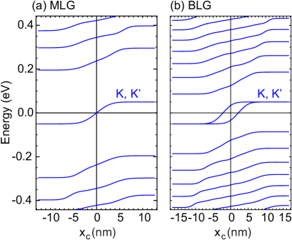
Figure A1: Energy levels of an n-p junction of a pristine (a) MLG and (b) BLG as a function of the center of the cyclotron orbit $x_{c}$ obtained from analytical results.

The two independent solutions of Eq. (A6) are the parabolic cylinder functions $D_{\nu}(z)$ and $D_{\nu}(-z)$ which vanish in the limit $z\rightarrow\infty$ and $z\rightarrow-\infty$, respectively. The other spinor component $\psi^{K}_{A}(z)$ can be obtained from the Schrödinger equation and by employing the relations

$$b^{{\dagger}}D_{\nu}(z)=\mathrm{sgn}(z)D_{\nu+1}(z),$$

$$bD_{\nu}(z)=\mathrm{sgn}(z)\nu D_{\nu-1}(z),$$ (A8)

where $\mathrm{sgn}(z)$ is the sign function.

Thus the spinor components in the MLG region where $x<0$ is given by

$$\left(\begin{array}[]{c}\psi^{K}_{A}(x)\\ \psi^{K}_{B}(x)\\ \end{array}\right)=C\left(\begin{array}[]{c}\mathrm{i}\,(\varepsilon-v_{1})D_{\nu-1}(-z)\\ D_{\nu}(-z)\end{array}\right),$$ (A9)

with $C$ being the normalization constant. The wave function at the $K^{\prime}$ valley can be obtained by $[\psi^{K^{\prime}}_{A},\psi^{K^{\prime}}_{B}]=[\psi^{K}_{B},\psi^{K}_{A}]$.

The BLG region can be described in terms of four sublattices, labeled $A1$, $B1$, for the lower layer and $A2$, $B2$, for the upper layer. We only include the coupling between two atoms stacked on top of each other, i.e., $B1$ and $A2$ [see Fig. 1], and ignore the small contributions of the other interlayer couplings. In the vicinity of the $K$ valley, the effective Hamiltonian is Koshino2010 ; McCann2006

$$\mathcal{H}^{K}_{\mathrm{BLG}}=\left(\begin{array}[]{cccc}V_{2}&v_{F}\pi_{-}&0&0\\ v_{F}\pi_{+}&V_{2}&\gamma_{1}&0\\ 0&\gamma_{1}&V_{2}&v_{F}\pi_{-}\\ 0&0&v_{F}\pi_{+}&V_{2}\\ \end{array}\right),$$ (A10)

where $\gamma_{1}$ is the nearest-neighbor interlayer hopping term and $V_{2}$ is the potential applied to the BLG region.

Solving the Schrödinger equation (A2) for the four-component envelope function $\mathbf{\Phi}^{K}(\mathbf{r})=(\phi^{K}_{A1},\phi^{K}_{B1},\phi^{K}_{A2},\phi^{K}_{B2})^{T}\mathrm{e}^{\mathrm{i}\,k_{y}y}$ and using the relations (Appendix) we obtain

$$\left(\begin{array}[]{c}\phi^{K}_{A1}(x)\\ \phi^{K}_{B1}(x)\\ \phi^{K}_{A2}(x)\\ \phi^{K}_{B2}(x)\\ \end{array}\right)=\sum_{\mu=\pm} C_{\mu}\left(\begin{array}[]{c}-\mathrm{i}\,[\tilde{\gamma}_{1}\varepsilon^{\prime}\nu_{\mu}/(\varepsilon^{\prime 2}-\nu_{\mu})]D_{\nu_{\mu}-1}(z)\\ \ [\tilde{\gamma}_{1}\varepsilon^{\prime 2}/(\varepsilon^{\prime 2}-\nu_{\mu})]D_{\nu_{\mu}}(z)\\ \varepsilon^{\prime}D_{\nu_{\mu}}(z)\\ \mathrm{i}\,D_{\nu_{\mu}+1}(z)\end{array}\right),$$ (A19)

where $C_{\mu}$ is normalization constant, $\tilde{\gamma}_{1}=\gamma_{1}/E_{0}$, $\varepsilon^{\prime}=\varepsilon-v_{2}$ with $v_{2}=V_{2}/E_{0}$, and

$$\nu_{\mu}=\frac{1}{2}\Big{(}-1+2\varepsilon^{\prime 2}+\mu\sqrt{1+4\tilde{\gamma_{1}}^{2}\varepsilon^{\prime}}\,\Big{)}.$$ (A20)

The wave function at the $K^{\prime}$ valley can be obtained by $[\psi^{K^{\prime}}_{A1},\psi^{K^{\prime}}_{B1},\psi^{K^{\prime}}_{A2},\psi^{K^{\prime}}_{B2}]=[\psi^{K}_{B2},\psi^{K}_{A2},\psi^{K}_{B1},\psi^{K}_{A1}]$.

The boundary conditions at $x=0$ for each interface are Nakanishi2010 :

$$\text{ZZ1}\left\{\!\!\begin{array}[]{l}\phi^{\tau}_{A1}(z_{0})=\psi^{\tau}_{A}(z_{0}),\\ \phi^{\tau}_{B1}(z_{0})=\psi^{\tau}_{B}(z_{0}),\\ \phi^{\tau}_{B2}(z_{0})=0,\end{array}\right.\quad\text{ZZ2}\left\{\!\!\begin{array}[]{l}\phi^{\tau}_{A1}(z_{0})=\psi^{\tau}_{A}(z_{0}),\\ \phi^{\tau}_{B1}(z_{0})=\psi^{\tau}_{B}(z_{0}),\\ \phi^{\tau}_{A2}(z_{0})=0,\end{array}\right.$$

where $\tau=K$ or $K^{\prime}$ and $z_{0}=-\sqrt{2}~{}x_{c}/l_{B}\equiv z(x=0)$.

The above conditions for two interfaces in each valley lead to a system of equations from which the eigenvalues are obtained by setting the determinant of the coefficients to zero. Solving such determinants numerically, one can obtain eigenvalues as a function of, e.g., cyclotron orbit $x_{c}$, as presented in Figs 2(e,f) and 3(b,d).

Using the analytical results, we also plot the energy levels for the n-p junctions of pure MLG and BLG structures in Figs. A1(a) and A1(b), respectively. As mentioned in the main text, one can clearly see one and two (valley degenerate) edge channels along the n-p junction in the bipolar regime for MLG and BLG structures, respectively.

References

- (1) D. A. Abanin and L. S. Levitov, Science 317, 641 (2007).
- (2) J. R. Williams, L. DiCarlo, and C. M. Marcus, Science 317, 638 (2007).
- (3) B. Huard, J. A. Sulpizio, N. Stander, K. Todd, B. Yang, and D. Goldhaber-Gordon, Phys. Rev. Lett. 98, 236803 (2007).
- (4) B. Özyilmaz, P. Jarillo-Herrero, D. Efetov, D. A. Abanin, L. S. Levitov, and P. Kim, Phys. Rev. Lett. 99, 166804 (2007).
- (5) J. Tworzydło, I. Snyman, A. R. Akhmerov, and C. W. J. Beenakker, Phys. Rev. B 76, 035411 (2007).
- (6) N. Myoung and H. C. Park, Phys. Rev. B 96, 235435 (2017).
- (7) L. Trifunovic and P. W. Brouwer, Phys. Rev. B 99, 205431 (2019).
- (8) N. Myoung, H. Choi, and H. C. Park, Carbon 157, 578 (2020).
- (9) Y. Ji, Y. Chung, D. Sprinzak, M. Heiblum, D. Mahalu, and H. Shtrikman, Nature (London) 422, 415 (2003).
- (10) S. Morikawa, S. Masubuchi, R. Moriya, K. Watanabe, T. Taniguchi, and T. Machida, Appl. Phys. Lett. 106, 183101 (2015).
- (11) D. S. Wei, T. van der Sar, J. D. Sanchez-Yamagishi, K. Watanabe, T. Taniguchi, P. Jarillo-Herrero, B. I. Halperin, and A. Yacoby, Sci. Adv. 3, e1700600 (2017).
- (12) P. Makk, C. Handschin, E. Tóvári, K. Watanabe, T. Taniguchi, K. Richter, M.-H. Liu, and C. SchÖnenberger, Phys. Rev. B 98, 035413 (2018).
- (13) M. Jo, P. Brasseur, A. Assouline, G. Fleury, H.-S. Sim, K. Watanabe, T. Taniguchi, W. Dumnernpanich, P. Roche, D. C. Glattli, N. Kumada, F. D. Parmentier, and P. Roulleau, Phys. Rev. Let. 126, 146803 (2021).
- (14) C. P. Puls, N. E. Staley, and Y. Liu, Phys. Rev. B 79, 235415 (2009).
- (15) J. Tian, Y. Jiang, I. Childres, H. Cao, J. Hu, and Y. P. Chen, Phys. Rev. B 88, 125410 (2013).
- (16) W. Yan, S.-Y. Li, L.-J. Yin, J.-B. Qiao, J.-C. Nie, and L. He, Phys. Rev. B 93, 195408 (2016).
- (17) F. Zhao, L. Xu, and J. Zhang J. Phys.: Condens. Matter 28, 185001 (2016).
- (18) M. Du, Luojun Du, N. Wei, W. Liu, X. Bai, and Z. Sunac, Nanoscale Adv. 3, 399 (2021).
- (19) M. Koshino, T. Nakanishi, and T. Ando, Phys. Rev. B 82, 205436 (2010).
- (20) L. V. Litvin, H.-P. Tranitz, W. Wegscheider, and C. Strunk, Phys. Rev. B 75, 033315 (2007).
- (21) E. Bieri, M. Weiss, O. Göktas, M. Hauser, C. Schönenberger, and S. Oberholzer, Phys. Rev. B 79, 245324 (2009).
- (22) E. Bocquillon, V. Freulon, J.-M. Berroir, P. Degiovanni, B. Plaçais, A. Cavanna, Y. Jin, and G. Fève, Science 339, 1054 (2013).
- (23) M. Henny, S. Oberholzer, C. Strunk, T. Heinzel, K. Ensslin, M. Holland, and C. Schöenenberger, Science 284, 296 (1999).
- (24) W. D. Oliver, J. Kim, R. C. Liu, and Y. Yamamoto, Science 284, 299 (1999).
- (25) K. T. Law, D. E. Feldman, and Y. Gefen, Phys. Rev. B 74, 045319 (2006).
- (26) D. E. Feldman and A. Kitaev, Phys. Rev. Lett. 97, 186803 (2006).
- (27) A. Bid, N. Ofek, M. Heiblum, V. Umansky, and D. Mahalu, Phys. Rev. Lett. 103, 236802 (2009).
- (28) B. Yurke and D. Stoler, Phys. Rev. A 46, 2229 (1992).
- (29) P. Samuelsson, E. V. Sukhorukov, and M. Büttiker, Phys. Rev. Lett. 92, 026805 (2004).
- (30) R. Peierls, Z. Phys. 80, 763 (1933).
- (31) S. Datta, Electronic transport in mesoscopic systems (Cambridge university press, 1997).
- (32) C. W. Groth, M. Wimmer, A. R. Akhmerov, X. Waintal, Kwant: a software package for quantum transport, New J. Phys. 16, 063065 (2014).
- (33) M.-H. Liu, P. Rickhaus, P. Makk, E. Tóvári, R. Maurand, F. Tkatschenko, M. Weiss, C. Schönenberger, and K. Richter, Phys. Rev. Lett. 114, 036601 (2015).
- (34) D. Cabosart, A. Felten, N. Reckinger, A. Iordanescu, S. Toussaint, S. Faniel, and B. Hackens, Nano Lett. 17, 1344 (2017).
- (35) K. S. Novoselov, A. K. Geim, S. V. Morozov, D. Jiang, M. I. Katsnelson, I. V. Grigorieva, S. V. Dubonos, and A. A. Firsov, Nature (London) 438, 197 (2005).
- (36) G. M. Rutter, S. Jung, N. N. Klimov, D. B. Newell, N. B. Zhitenev, and J. A. Stroscio, Nat. Phys. 7, 649 (2011).
- (37) M. Mirzakhani, M. Zarenia, P. Vasilopoulos, S. A. Ketabi, and F. M. Peeters, Phys. Rev. B 96, 125430 (2017).
- (38) C. W. J. Beenakker, Rev. Mod. Phys. 80, 1337 (2008).
- (39) Tables of Integrals, Series, and Products, I. S. Gradshteyn, and I. M. Ryzhik, (6th ed. San Diego, CA: Academic Press, 2000), p. 989.
- (40) E. McCann and V. I. Fal’ko, Phys. Rev. Lett. 96, 086805 (2006).
- (41) T. Nakanishi, M. Koshino, and T. Ando, Phys. Rev. B 82, 125428 (2010).