Re-Examining Calibration: The Case of Question Answering

Abstract

For users to trust model predictions, they need to understand model outputs, particularly their confidence—calibration aims to adjust (calibrate) models’ confidence to match expected accuracy. We argue that the traditional calibration evaluation does not promote effective calibrations: for example, it can encourage always assigning a mediocre confidence score to all predictions, which does not help users distinguish correct predictions from wrong ones. Building on those observations, we propose a new calibration metric, MacroCE, that better captures whether the model assigns low confidence to wrong predictions and high confidence to correct predictions. Focusing on the practical application of open-domain question answering, we examine conventional calibration methods applied on the widely-used retriever-reader pipeline, all of which do not bring significant gains under our new MacroCE metric. Toward better calibration, we propose a new calibration method (ConsCal) that uses not just final model predictions but whether multiple model checkpoints make consistent predictions. Altogether, we provide an alternative view of calibration along with a new metric, re-evaluation of existing calibration methods on our metric, and proposal of a more effective calibration method. 

1 Introduction

While large pretrained language models have conquered many downstream tasks Devlin et al. (2019); Brown et al. (2020), it is sometimes unclear when we should trust them since they often produce false Lin et al. (2022) or hallucinated Maynez et al. (2020) predictions. This is important for both model deployment—where low-confidence outputs can be censored—and end users who need to know whether to trust a model output. The solution is to make sure that models provide reliable confidence estimates so that we can abstain from wrong predictions and trust the right ones. The prerequisite for such abstention is Model Calibration: making the confidence represent the actual likelihood of being correct Niculescu-Mizil and Caruana (2005); Naeini et al. (2015). Past work proposes post-hoc approaches to calibrate model onfidence such as temperature scaling Guo et al. (2017), and can effectively calibrate multi-class classification, evaluated by the expected calibration error (ece) metric.

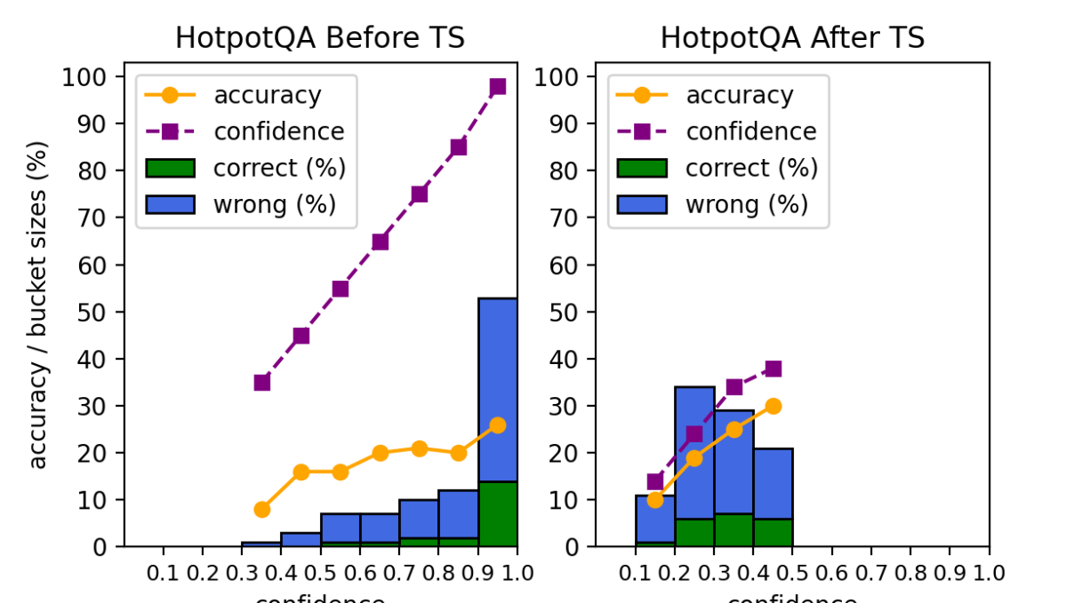
Figure 1: Distribution of predictions on HotpotQA in an ood setting. We put predictions within the same confidence range into the same bucket (10 fixed-range buckets), compute the average confidence and accuracy within each bucket. The x-axis represents the confidence range of each bucket, the y-axis represents the average answer accuracy for the dashed line plot and represents the relative bucket sizes for the histogram. Before calibration, most predictions have overly high confidence. After temperature scaling, all predictions’ confidence values are scaled to become closer to the overall answer accuracy (24.5). Both correct (green bars) and wrong predictions (blue bars) are mixed in the same buckets, making them hard to distinguish.

We re-examine calibration and apply it to a complex task with real-world applications: open-domain question answering (odqa; Chen et al., 2017). The task takes an input question, retrieves evidence passages from a large corpus such as Wikipedia, and then returns an answer string. Unlike classification, odqa is a pipeline with multiple components: a passage retriever followed by a reader. This complexity is both typical of modern machine learning systems and poses additional challenges. We explore adapting the calibration methods for the retriever-reader odqa models on both in-domain and out-of-domain (ood) settings. Using the commonly used temperature scaling (ts) method on odqa, models get lower ece, similar to previous findings on multi-class classification tasks Guo et al. (2017); Desai and Durrett (2020).

However, we argue that low ece does not correspond to useful calibration: in fact, it under-estimates the true calibration errors due to its bucketing mechanism. ece measures the difference between the confidence and expected accuracy by splitting the confidence values into buckets, taking an average confidence and an average accuracy of each bucket and marginalizing over their differences. However, this allows models with middling confidence to win on the ece metric. For instance, temperature scaling assigns all predictions in the range $[0.1,0.5)$ on HotpotQA (Figure 1), which is not useful for users separating correct and wrong predictions because the confidence values are all in a similar range. Moreover, the bucketing mechanism causes a cancellation effect where over-confident and under-confident predictions are bucketed together and averaged out, hiding the instance-level calibration errors.

We propose Macro-average Calibration Error (MacroCE) as an alternative metric that directly focuses on distinguishing correct from wrong predictions (Section 4.2). MacroCE removes the bucketing mechanism and sums calibration error at the instance level. It also takes equal consideration of correct and wrong predictions through macro-averaging in order to be insensitive to the accuracy level (e.g., when the accuracy is very low, simply lowering confidence on all predictions would lower ece, but not MacroCE). MacroCE is insensitive to accuracy shifts, successfully satisfying the desiderata for a stable calibration metric (Nixon et al., 2019). We also show that this metric flips the conclusion from the previous section based on ece—four existing calibration methods, including temperature scaling—the ece winner—do not lead to improvements in MacroCE (Section 4).

To address this shortcoming, we propose a new method, ConsCal, which tracks whether the model makes consistent correct predictions over different checkpoints during training. The intuition is that if the same correct prediction is consistent throughout the training trajectory, then it could serve as a strong sign that the model is confident about the prediction. ConsCal significantly improves MacroCE on both in-domain and ood evaluation (Section 5), including when downstream users must validate model predictions (Section 5).

In summary, our contributions are:

We thoroughly study calibration in the odqa setting, an under-explored real-world problem involving complex pipelines. We find that existing calibration methods like ts achieve very low ece; however, it does not capture if the model effectively distinguishes correct and wrong predictions.

We propose a better metric MacroCE, which captures models’ ability to distinguish correct and wrong predictions without being sensitive to the absolute model accuracy. Four different calibration methods known to be effective on ece are ineffective on MacroCE.

We introduce a new calibration method (ConsCal) that uses the consistency of model predictions to estimate confidence, significantly reducing MacroCE and outperforming all previous baselines.

Together, we provide an alternative view of calibration, re-evaluation of existing calibration methods and a proposal of a better calibration method based on our new viewpoint.

2 Background

This section reviews the existing calibration framework, the associated ece metric, and the commonly used temperature scaling method that effectively optimizes the ece metric.

2.1 Bucketing-based Calibration and ECE

Under the existing calibration framework, a model is “perfectly calibrated” if the prediction probability (i.e., confidence) reflects the ground truth likelihood (Niculescu-Mizil and Caruana, 2005). Specifically, given the input $x$, the ground truth $y$ and the prediction $\hat{y}$, the perfectly calibrated confidence $\mathrm{Conf}(x,\hat{y})$ will satisfy: $\forall p\in[0,1],P(\hat{y}=y\,|\,\mathrm{Conf}(x,\hat{y})=p)=p$.

Prior work Guo et al. (2017) evaluates calibration with Expected Calibration Error (ece), where N model predictions are bucketed into $M$ bins and predictions within the same confidence range are put into the same bucket. Let $B_{m}$ be the $m$-th bin of $(x,y,\hat{y})$ triples, the accuracy $\mathrm{Acc}(B_{m})$ measures how many instances in the bin are correct,

$$\mathrm{Acc}(B_{m})=\frac{1}{|B_{m}|}\sum_{i=1}^{|B_{m}|}\mathbb{I}(y=\hat{y}),\\$$

where $\mathrm{|B_{m}|}$ is the number of examples in the $m$-th bin, and $\mathrm{Conf}(B_{m})$ computes the average confidence in the bin,

$$\mathrm{Conf}(B_{m})=\frac{1}{|B_{m}|}\sum_{i=1}^{|B_{m}|}\mathrm{Conf}(x,\hat{y}).\\$$

Finally ece measures the difference in expectation between confidence and accuracy over all bins,

$$\mathrm{ECE}=\sum^{M}_{m=1}\frac{|B_{m}|}{N}|\mathrm{Acc}(B_{m})-\mathrm{Conf}(B_{m})|.\\$$

Most work uses equal-width buckets: a triple $(x,y,\hat{y})$ with $\frac{m}{M}\leq\mathrm{Conf}(x,\hat{y})\leq\frac{m+1}{M}$ is assigned to the $m$-th bin. Minderer et al. (2021) and Nguyen and O’Connor (2015) also used equal-mass binning: predictions are sorted by their confidence values and $\frac{N}{M}$ triples are assigned to each bin. We find little difference between equal-width and equal-mass binning ece results (Table 4), and so we will use the more common equal-width binning in the rest of our experiments.

2.2 Temperature Scaling

Without calibration, the confidence is often too high (or less commonly, too low): it thus needs to be scaled up or down. A widely-used calibration method is temperature scaling (Guo et al., 2017), which uses a single scalar parameter called the temperature $\tau$ to scale the confidence. The temperature value is optimized on the dev set. Given the set of candidate answers $\mathcal{C}$ and the logit value $\mathbf{z}\in\mathbb{R}^{|\mathcal{C}|}$ associated with the prediction $\hat{y}$, the confidence for the prediction $\hat{y}$ that is the $j$-th label in $\mathcal{C}$ is:

$$\mathrm{Softmax}\left(\frac{\mathbf{z}}{\tau}\right)_{j}.$$

For classification, the temperature scalar $\tau$ is tuned to optimize negative log likelihood (nll) on the dev set. Temperature scaling only changes the confidence—not the predictions—so the model’s accuracy remains the same.

3 Calibration in Open-Domain Question Answering

This section adapts the bucketing-based calibration framework for multi-class classification to odqa and evaluates this calibration method on multiple qa benchmarks, both in- and out-of-domain.

3.1 The ODQA Model

We use the model from Karpukhin et al. (2020), consisting of retrieval and reader components. The retrieval model is a dual encoder that computes the vector representation of the question and each Wikipedia passage, and returns the top-$K$ passages with the highest inner product scores between the question vector and the passage vector. The reader model is a bert-based (Devlin et al., 2019) span extractor. Given the concatenation of the question and each retrieved passage, it returns three logit values, representing the passage selection score, the start position score and the end position score respectively. These three logits are produced by three different classification heads on top of the final bert representations. More precisely,

$$\mathbf{H}_{i} =\mathrm{BERT}(q,p_{i})\in\mathbb{R}^{h\times L},$$

$$z^{\mathrm{psg}}(i) =\left(\mathbf{H}_{i}\right)_{\texttt{[CLS]}}\mathbf{w}_{\mathrm{psg}}\in\mathbb{R},$$

$$z^{\mathrm{start}}(i,s) =\left(\mathbf{H}_{i}\mathbf{w}^{\mathrm{start}}\right)_{s}\in\mathbb{R},$$

$$z^{\mathrm{end}}(i,e) =\left(\mathbf{H}_{i}\mathbf{w}^{\mathrm{end}}\right)_{e}\in\mathbb{R},$$

where $\mathbf{w}_{\mathrm{psg}},\mathbf{w}^{\mathrm{start}},\mathbf{w}^{\mathrm{end}}\in\mathbb{R}^{h}$ are trainable parameters.

3.2 Temperature Scaling For ODQA

The formulation of odqa is unlike conventional multi-class classification since it involves both the retriever and reader, leaving the question of what we should base the confidence score on. To adapt temperature scaling on odqa, we take the set of top span predictions as our candidate set $\mathcal{C}$. Specifically, we compute the raw score for each candidate span and then apply softmax over $\mathcal{C}$ to convert the raw span scores into probabilistic confidence values. We explore two possible implementations: Joint Calibration considers both passage and span scores; Pipeline Calibration selects highest scored passage first, then calibrates on span scores only.

Joint Calibration.

Given the top $k=10$ retrieved passages for each question and for each passage’s top $n=10$ spans, we have an answer set of $n\times k=100$ spans per question. We score each candidate by adding its passage, span start and span end score:

$$z^{\mathrm{start}}(\hat{i},s)+z^{\mathrm{end}}(\hat{i},e)+z^{\mathrm{psg}}(i).$$

We then apply temperature scaling to the predicted logits and the confidence becomes:

$$\mathrm{Softmax}_{(i,s,e)\in\mathcal{C}}\left(\frac{z^{\mathrm{psg}}(i)+z^{\mathrm{start}}(i,s)+z^{\mathrm{end}}(i,e)}{\tau}\right)$$

Note that for odqa, the number of correct answers in the candidate set $\mathcal{C}$ varies (zero, one, or more). Hence, the temperature scalar $\tau$ is tuned to optimize dev set ece instead of nll.

Pipeline Calibration.

We choose the passage with the highest passage selection score $i_{\mathrm{max}}=\mathrm{argmax}_{1\leq i\leq K}z^{\mathrm{psg}}(i)$ and then define the span score $S(s,e,i)$ as

$$\left(z^{\mathrm{start}}(\hat{i},s)+z^{\mathrm{end}}(\hat{i},e)\right)\mathbb{I}[i=i_{\mathrm{max}}].$$

In this case, we only keep the top $n=10$ spans from the top passage for each question. Like Joint Calibration, we apply temperature scaling to the predicted span logits and the confidence is:

$$\mathrm{Softmax}_{(i,s,e)\in\mathcal{C}}\left(\frac{z^{\mathrm{start}}(i,s)+z^{\mathrm{end}}(i,e)}{\tau}\right).$$

		Section 3		Section 4
Model	TS	EM↑	ECE↓	ICE↓	MacroCE↓
NQ
Joint	-	32.9	27.1	47.8	43.6
Joint	✓	32.9	4.0	37.4	42.5
Pipeline	-	34.1	48.2	55.1	44.2
Pipeline	✓	34.1	2.7	39.7	44.4
NQ $\rightarrow$ HotpotQA
Joint	-	24.9	41.0	54.7	45.7
Joint	✓	24.9	12.5	40.3	45.5
Pipeline	-	22.6	59.6	65.9	47.4
Pipeline	✓	22.6	8.4	37.9	47.7
NQ $\rightarrow$ TriviaQA
Joint	-	33.6	25.4	48.6	45.1
Joint	✓	33.6	6.4	38.4	44.3
Pipeline	-	34.2	48.2	54.5	43.7
Pipeline	✓	34.2	6.1	39.2	44.6
NQ $\rightarrow$ SQuAD
Joint	-	12.4	41.7	48.5	39.5
Joint	✓	12.4	12.4	26.6	39.7
Pipeline	-	12.2	62.7	65.1	41.4
Pipeline	✓	12.2	13.5	29.1	43.9

Table 1: In-domain and ood calibration results. Joint and Pipeline refer to whether the candidate set consists of top answer candidates from all top-10 retrieved passages or just the top-1 retrieved passage. All numbers are multiplied by 100 for better readability throughout the paper. em: higher is better. Calibration errors: lower is better. Best calibration result in each group is in bold. Across all settings, temperature scaling significantly improves ece but not MacroCE, highlighting the difference between these calibration metrics. Also, ood incurs higher calibration errors.

3.3 Temperature Scaling Results

We experiment the above temperature scaling methods on both in-domain and ood settings, since Desai and Durrett (2020); Jiang et al. (2021) argue that ood calibration is more challenging than in-domain calibration. We use NaturalQuestions (Kwiatkowski et al., 2019, nq) as the in-domain dataset, and SQuAD (Rajpurkar et al., 2016), TriviaQA (Joshi et al., 2017) and HotpotQA (Yang et al., 2018) as the out-of-domain datasets. We tune hyper-parameters on the in-domain nq dev set. We report exact match (em) for answer accuracy and ece for calibration results.

Without calibration, both joint and pipeline approaches have high ece scores, and the pipeline approach incurs higher out-of-the-box calibration error (Table 1). Applying temperature scaling significantly lowers ece in all cases, including both in-domain and ood settings. As expected, ood settings incur higher ece than the in-domain setting even after calibration. However, in the next section, we challenge this “success” by re-examining the bucketing mechanism in ece computation.

4 Flaws in ECE and Better Alternatives

This section takes a closer look at the model accuracy and confidence, and illustrate how ece is misleading in evaluating model calibration. We provide complementary views of calibration and propose a new calibration metric as an alternative.

4.1 What’s Wrong With ECE?

We illustrate the ece problem with a case study on HotpotQA; similar trends surface for other datasets (Appendix F). The uncalibrated model is over-confident (Figure 1): the confidence is higher than the accuracy. After temperature scaling, the accuracy and confidence converge, reducing ece. However, this over-estimates the effectiveness of temperature scaling for two reasons. First, most instances are assigned similar confidence. All predictions have a confidence score between 0.1 and 0.5, not giving useful cues except that the model is not confident on most predictions. This is not ideal since, if there were examples we could trust or abstain, an ideal calibration metric should recognize such scenarios and encourage the calibrator to differentiate correct and wrong predictions. Second, bucketing causes cancellation effects, ignoring instance-level calibration error. Many predictions are clustered in the same buckets. As a result, there are many over-confident and under-confident predictions in the same bucket and are averaged to become closer to the average accuracy. 

The Need for An Alternative View.

The above issues are because ece only measures the expectation where the aim is to match the confidence with the expected accuracy. However, this goal can be trivially achieved by simply outputting the similar confidence for all predictions that match the expected accuracy, as in the case of temperature scaling, which is not useful because users cannot easily use such confidence scores to make abstaining judgments. Hence, we propose an alternative view of calibration where the goal is to maximally differentiate correct and wrong predictions. We argue that achieving this goal would bring better practical values for real use cases. Toward this end, we propose a new calibration metric that aligns closely with our objective.

4.2 New Metric: MacroCE

We propose alternative metrics that remove the bucketing mechanism to prevent the above problems. We consider two such metrics—ice and MacroCE. We evaluate their robustness to various distribution shifts, and propose to use MacroCE as the main metric.

Instance-level Calibration Error (ice)

accumulates the calibrator error of each individual prediction and takes an average. Formally,

$$\mathrm{ICE}=\frac{1}{n}\sum^{n}_{i=1}|\mathbb{I}(y_{i}=\tilde{y}_{i})-\mathrm{Conf}(x_{i},\tilde{y}_{i})|.$$

ice is similar to the Brier Score Brier (1950) except that we are marginalizing over the absolute difference between accuracy and confidence of predictions, instead of squared errors.

While ice and Brier Score prevent the issues brought by bucketing, it incurs another issue: they can be easily dominated by the majority label classes. For example, if the model achieves high accuracy, always assigning a high confidence can get low ice and Brier Score because the wrong predictions contribute very little to the overall calibration error (we will empirically show this in the following experiments). This is undesirable because even when the wrong predictions are rare, mistrusting them can still cause severe harms to users. To address this, we additionally perform macro-averaging of the calibration errors on correct and wrong predictions, and we name this metric MacroCE.

Macro-average Calibration Error (MacroCE)

considers instance-level errors, but it takes equal consideration of correct and wrong predictions made by the model. Specifically, it calculates a macro-average over calibration errors on correct predictions and wrong predictions:

$$\mathrm{ICE_{pos}} =\frac{1}{n_{p}}\sum^{n_{p}}_{i=1}(1-\mathrm{Conf}(x_{i},\tilde{y}_{i})),\forall\tilde{y}_{i}=y_{i},$$

$$\mathrm{ICE_{neg}} =\frac{1}{n_{n}}\sum^{n_{n}}_{i=1}(\mathrm{Conf}(x_{i},\tilde{y}_{i})-0),\forall\tilde{y}_{i}\neq y_{i},$$

$$\mathrm{MacroCE} =\frac{1}{2}(\mathrm{ICE_{pos}}+\mathrm{ICE_{neg}}).$$

Where $n_{p}$ and $n_{n}$ are the number correct and wrong predictions. Ideal calibration metrics should be insensitive to shifts in accuracy (Nixon et al., 2019) and stably reveal models’ calibration in all situations. We examine the robustness of these metrics.

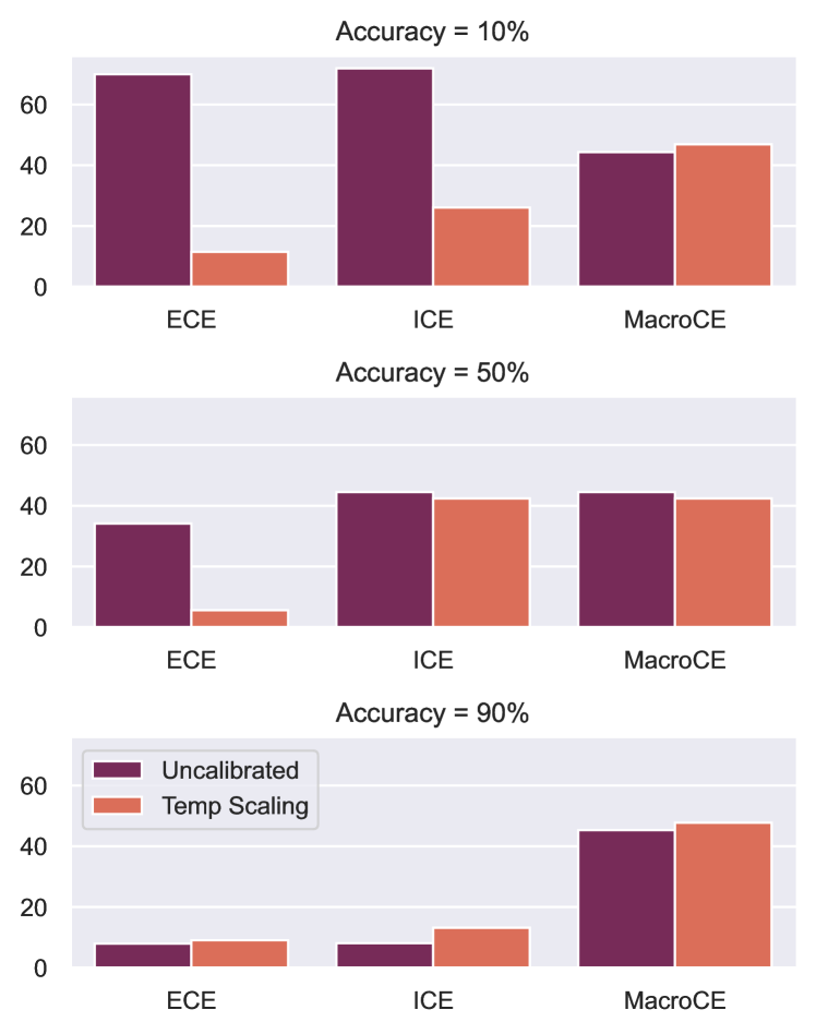
Figure 2: Calibration results where we re-sample the predictions to vary the model accuracy (10%, 50%, 90%; same on both dev and test sets). Uncalibrated ece and ice results differ largely at different accuracy (i.e., highly sensitive to accuracy), while MacroCE stays much more stable.

Temperature Scaling at Different Accuracy Levels

We re-sample the data to very the model accuracy and examine the effect of temperature scaling at different accuracy levels. According to Table 2, before calibration, the ece score decreases with higher model accuracy, since higher accuracy matches the over-confidence predictions and gets rewarded by low ece score. Such finding also applies to ice, since the majority of predictions are correct, the impact of negative predictions with over-confidence is marginal. MacroCE results remain stable across all accuracy levels. As model accuracy increases, ice_pos decreases and ice_neg increases. MacroCE captures the trade-off and implies the model remains poorly calibrated.

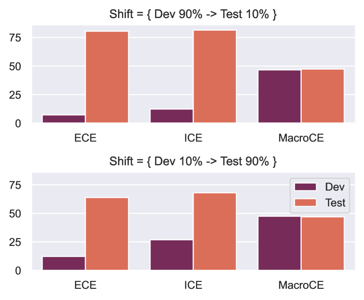
Figure 3: Calibration results when training and test accuracy are different. In the first case, we tune the temperature value on a dev set with only 10% correct predictions and a test set with 90% correct predictions, and we reverse the setup in the second case. ece and ice change significantly under such accuracy shifts even though the underlying model is the same. In contrast, only MacroCE is stable under train-test accuracy shifts as desired.

Temperature Scaling under Accuracy Shift

We consider the setting where there is a large difference between the dev and test set accuracy. In particular, we consider the cases where we: 1) tune temperature on a development set with 90% accuracy and evaluate on a test set with 10% accuracy; and 2) tune temperature on a development set with 10% accuracy and evaluate on a test set with 90% accuracy. ece and ice are sensitive to the model accuracy but MacroCEis not (Table 3). Temperature scaling selects a low temperature scalar on the highly accurate development set which does not transfer to the test set with low accuracy, which indicates that temperature tuning does not hold against subpopulation shift. MacroCE reflects the poor calibration of the model on both cases, insensitive to the shift..

Both experiments indicate that MacroCE is a more reliable calibration evaluation metric. We thus focus on MacroCE evaluation throughout the rest of the paper.

4.3 Re-Evaluating Calibration with New Metrics

Table 1 compares calibration results under ece (with both equal-width and equal-width binning), ice and MacroCE results for all experiment settings described in Section 3.3. Temperature scaling significantly improves ece and ice with both joint and pipeline calibration, but it does not improve MacroCE. Moreover, ece and ice are very sensitive to accuracy shifts. When transferring from nq to HotpotQA and SQuAD where the accuracy drops, there is significant increase in ece and ice (before temperature scaling), but MacroCE stays high despite such shifts.

5 Toward Better Calibration Methods

This section reviews existing calibration methods other than temperature scaling as baselines—including feature based classifier, neural reranker and label smoothing (Section 5.1)—and introduces our new calibration method based on model consistency throughout training trajectory (ConsCal; Section 5.2). All existing methods do not lower MacroCE, while ConsCal significantly improves MacroCE (Section 5.3).

	iid (nq)			ood (HotpotQA)
Calibrator	EM	ECE	MacroCE	EM	ECE	MacroCE
No Calibration	35.2	30.4	44.5	24.5	44.4	46.2
Binary Baseline	35.2	38.0	53.2	24.5	38.6	44.4
Average Baseline	35.2	2.0	50.0	24.5	11.3	50.0
Temperature Scaling	35.2	4.7	42.5	24.5	13.7	45.6
Feature-based	36.5	52.3	45.0	21.8	62.4	46.9
Neural Reranker	37.6	58.6	41.0	26.5	51.4	47.0
Label Smoothing	36.1	29.4	45.6	23.6	44.7	46.8
Label Smoothing + TS	36.1	5.6	43.5	23.6	14.3	46.0
ConsCal w/o Training Dynamics	37.8	29.0	32.2	25.7	31.9	41.0
ConsCal	35.2	33.1	31.7	24.5	41.3	39.0

Table 2: Results of existing calibration methods (Section 5.1) and ConsCal (Section 5.2). ‘ConsCal w/o Training Dynamics’ is the ensemble-based method from Section 5.3. While some existing methods drastically reduce ece, none of them significantly reduces MacroCE; on the other hand, ConsCal sets the new state-of-the-art on MacroCE both in-domain and out-of-domain (best results in bold). Different metrics give different ranking of methods, which further highlights the importance of using a reliable and informative metric.

5.1 Existing Calibration Baselines

Simple Baselines.

We begin with two simple baselines: Binary baseline assigns the top $t$% (dev set accuracy) confident predictions in the test set with confidence 1, otherwise 0. Average baseline assigns all test set predictions with the confidence value equal to the dev set accuracy.

Feature Based Classifier.

Prior work has trained a feature-based classifier to predict the correctness of outputs Zhang et al. (2021); Ye and Durrett (2022). We use SVM to train them as binary classifiers following prior work Kamath et al. (2020). We include a wide variety of features based on previous work Rodriguez et al. (2019) (features used are described in Appendix B). During inference time, we use the classifiers’ predicted probability of the test example being correct as its confidence.

Neural Reranker.

We train a neural reranker as an alternative to manual features. We adopt ReConsider Iyer et al. (2021) where we train a bert-large classifier by feeding in the concatenation of the question, passage, and answer span. Passing the raw logit through a sigmoid provides the confidence score.

Label Smoothing.

In addition to the post-hoc calibration methods above, another way of calibration is to train models that are inherently better calibrated, and a representative approach is label smoothing Pereyra et al. (2017); Desai and Durrett (2020). Label smoothing assigns the gold label probability $\alpha$ and the other classes $\frac{1-\alpha}{|Y|-1}$. We apply label smoothing on two components of the odqa pipeline: passage selection (where the first passage is gold, the rest $K-1$ are false); span selection (where the gold class is the correct answer start and end position and false classes are the other positions in the passage).

5.2 ConsCal: Calibration Through Consistency

The failure of temperature scaling under MacroCE implies that only relying on the final outputs from the qa model is not sufficient for calibration. This calls for additional cues that can reflect the model’s confidence. We propose to use the model’s consistency throughout training as a useful cue. We propose a simple calibration method called Consistency Calibration (ConsCal). ConsCal compares multiple model checkpoints throughout training and checks if the prediction is consistent. The intuition is that if the model during training always makes the same prediction, the model is confident about that prediction, and vice versa. This is inspired by Training Dynamics from Swayamdipta et al. (2020); while they originally use training dynamics to measure data difficulty, we use it to measure the confidence of the model predictions.

Specifically, given $N$ model checkpoints, we obtain the final model prediction $p$ based on the last checkpoint, then count the checkpoints that make the same prediction, and assign a confidence value 1 if the count is greater than a threshold $n$; otherwise 0. The threshold $n$ is a hyper-parameter chosen based on the development set. Apart from this binary confidence setting, we also explore assigning continuous confidence values based on checkpoint consistency. This continuous confidence gets slightly worse MacroCE than the binary version but improves on all previous baselines (Appendix B).

5.3 Experimental Results

Some existing calibration methods lower ece, including temperature scaling, the simple average baseline, and label smoothing (Table 2). In particular, the simple average baseline has the lowest ece both in-domain and ood. This confirms our earlier point that you can lower ece by assigning confidence values close to the accuracy for all predictions without any discrimination between correct and wrong predictions. However, none of these baselines reduces MacroCE.

ConsCal significantly lowers MacroCE, outperforming the previous best by 11% and 6% absolute in-domain and out-of-domain, respectively. This confirms the effectiveness of using consistency over different checkpoints throughout training. Notably, that ConsCal significantly outperforms the simple binary baseline highlights that binary confidence is not the reason for better MacroCE. Additional results in Appendix D compare the joint and pipeline approach (defined in section 3.2), which have similar MacroCE.

To analyse whether the gains of ConsCal are simply from ensembling multiple checkpoints, we compare with an additional baseline called ConsCal w/o Training Dynamics: we finetune the model $N$ times independently using different random seeds, obtain final predictions through majority vote, and compute the confidence scores as we did for ConsCal. We use the same $N$ ($N=5$) for both ConsCal and ConsCal w/o Training Dynamics. While this variant reduces MacroCE more than any of previous methods, its MacroCE values are still higher than ConsCal both in-domain and ood. This suggests that, while ensembling is one factor for reducing MacroCE, it is not the only factor—considering training dynamics remains important. We provide a qualitative example in Figure 4: the model changes its prediction in the last epochs – a cue to suggest low confidence via ConsCal.

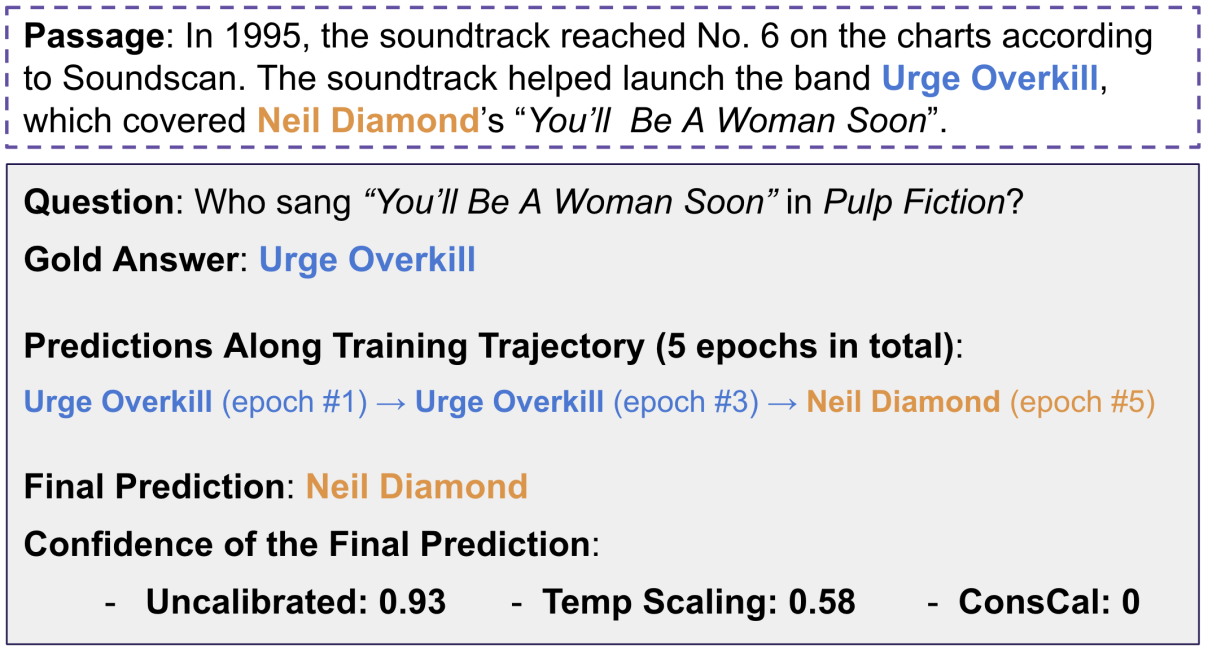
Figure 4: An example from nq where the final prediction is wrong. The original uncalibrated confidence is over-confident, while temperature scaling lowers it, it is still over-confident and could mislead users. ConsCal sets the confidence to 0 because predictions across checkpoints in the training trajectory are inconsistent—the model is confused between the specific performer and the original singer in this example.

	ECE	MacroCE	Precision	Recall	F1	Agreement ($\alpha$)
No Confidence	–	–	0.37	0.62	0.46	0.21
Raw Confidence	30.4	44.5	0.38	0.67	0.48	0.35
Temp Scaling	4.7	42.5	0.44	0.72	0.54	0.33
ConsCal	33.1	31.7	0.50	0.68	0.58	0.40
ConsCal  (Always Trust)	33.1	31.7	0.53	0.82	0.64	–

Table 3: We ask humans—given an estimate of confidence—whether they think a qa system is correct or not. The model accuracy on this sampled set is 35%. Apart from human ratings, we additionally show a baseline of always following ConsCal’s judgement in the last row. Showing the confidence significant improves human judgement, especially with ConsCal. Surprisingly, annotators sometimes do not trust and overrule ConsCal’s confidence scores, which results in worse F1 (second to last row). Furthermore, MacroCE  ranks ConsCal  as the best method, agreeing with human evaluation, while ece misleadingly favors temperature scaling.

5.4 Human Study

Finally, we investigate whether ConsCal improves user decision making—mimicing validating a search engine’s answer to a question—with a human study. We randomly sample 100 questions from the nq test set and present the questions to annotators along with the dpr-bert predictions. We ask annotators to judge the correctness of the model predictions under four settings: (1) show only questions and predictions without model confidence; (2) show the qa pairs along with raw model confidence without calibration; (3) show the qa pairs along with temperature scaled confidence; (4) show the qa pairs along with confidence calibrated by ConsCal. We recruit a total of twenty annotators (five annotators under each setting) on Prolific, each annotating 100 questions, with average compensation of $14.4/hour.

We measure the precision, recall, and F1 score of the human judgement. We also report Krippendorff’s alpha among the five annotators. Showing the confidence scores significantly improves human decision making (Table 3), and ConsCal helps achieve better F1 than temperature scaling. Interestingly, despite ConsCal providing binary confidence scores of 0 and 1, humans sometimes do not follow the confidence scores and “overrule” them. This actually leads to worse F1 than a baseline that always follows ConsCal’s confidence. Moreover, the ece metric ranks temperature scaling as best, contradicting human study results. Nevertheless, our MacroCE correctly ranks ConsCal as the best method, aligning with human judgement.

6 Related Work

This section reviews prior work on calibration metrics and methods that are relevant to nlp.

Calibration Metrics.

Brier Score Brier (1950) is one of the earliest calibration metrics that sums over squared errors between accuracy and confidence for all instances, but is only applicable to binary classification. Naeini et al. (2015) first use bucketing mechanisms to compute calibration errors, and propose metrics like ece and maximum calibration error (mce), Nguyen and O’Connor (2015) explore other bucketing mechanisms like equal-mass binning. Nixon et al. (2019) point out the flaws of the fixed range bucketing mechanism used by ece, and propose an adaptive bucketing mechanism as an alternative. We take inspiration from these prior analysis, identify the problems grounded in a more complex open-domain question answering task, and propose MacroCE to address the issues.

Calibration Methods.

Guo et al. (2017) first experiment various post-hoc calibration methods including temperature scaling, and Thulasidasan et al. (2019) find that mixup training improves the calibration of image classifier evaluated by the ece metric. Within nlp domain, previous works have explored calibration on various tasks, including multi-class classification Desai and Durrett (2020) and sequence tagging Nguyen and O’Connor (2015). In question answering, Kamath et al. (2020) propose the selective question answering setting that aims to abstain as few questions as possible while maintaining high accuracy. Toward this goal, later approaches Zhang et al. (2021); Ye and Durrett (2022) use featured based approach to train a binary classifier for deciding what questions to abstain. While selective question answering offers a way of measuring calibration, the scale of confidence values is not considered since abstention can be effective as long as correct predictions have higher confidence than wrong ones, regardless of the absolute scales. Concurrent work Dhuliawala et al. (2022) explores calibration for retriever-reader odqa, focusing on combining information from the retriever and reader. In addition to span-extraction qa, Jiang et al. (2021) and Si et al. (2022) also explore calibration for generative qa. However, these works use ece for evaluation.

7 Conclusion

This paper investigates calibration in the realistic application of odqa where users need to decide whether to trust the model prediction based on the confidence scores. Although confidence scores produced by existing calibration methods improves the popular ece metric, these confidence scores do not help distinguish correct and wrong predictions. We propose to use the MacroCE metric to remedy the flaws, and existing calibration methods fail on our MacroCE metric. We further propose a simple and effective calibration method ConsCal that leverages training consistency. Our human study confirms both the effectiveness of ConsCal as well as the alignment between MacroCE and human preference. Our work advocates and paves the path for user-centric calibration, and our ConsCal method is a promising direction for better calibration. Future work can adapt our calibration metric and method to more diverse tasks (such as generative tasks) and explore other ways to further improve user-centric calibration.

Limitations

We note several limitations of this paper and point to potential future directions to address them:

• MacroCE is motivated from a user-centric perspective where we want to maximally distinguish correct and wrong predictions. However, it is not the panacea for all use cases, e.g., in some applications, the confidence output might have to be mediocre to indicate the uncertainty of the output, rather than taking a stance as MacroCE encourages.

• Our experiments are focused on odqa and in particular, span-extraction models (we also showed similar findings on binary sentiment classification in Appendix F). While we expect most findings in this paper to hold for other models and tasks as well, this needs to be empirically verified in future work. In particular, one promising line for future work is to verify whether ConsCal also works well for text generation tasks and models.

Ethical Considerations

Data and Human Subjects

All datasets used in this paper are from existing public sources and we do not expect any violation of intellectual property or privacy. All human annotators that we recruited on Prolific are well-compensated and we did not receive any complaints from the annotators regarding the job (we do not perceive any possible harm on them either).

Broader Impact

We expect our study to have a positive impact on the safe deployment of AI applications. Our study is targeted towards the real-world application of question answering from a user-centric perspective. We make model predictions more trustworthy to users by providing well-calibrated confidence scores. This especially helps users avoid misleading wrong predictions which can cause serious troubles in real-life applications such as digital assistants and search engines. Our human study has also confirmed the advantages of our proposed metric and calibration method.

Appendix

Appendix A More Analysis on Calibration Metrics

Temperature Scaling with Different Temperature Scalars

We apply temperature scaling with varying temperature scalar $\tau$. According to Figure 5, as we increase the temperature value, the confidence scores decrease, and consequently ice_pos increases and ice_neg decreases. Meanwhile, MacroCE stays constant while ece changes drastically, which reflects the flaw of temperature scaling: a single temperature value cannot improve calibration for both correct and wrong predictions simultaneously. Such flaw is only captured by MacroCE.

ECE with Equal-Width and Equal-Mass Binning

We compare measuring calibration with equal-width bucketed ECE and equal-mass bucketed ECE in Table 4. We find that both variants of ECE give similar results on all experiment settings, and both of them show contrary conclusions than MacroCE (e.g., they both underestimate the calibration errors of temperature scaling in OOD settings).

Calibration Results at Different Accuracy

In Table 5, we show the numerical results of ece, ice, and MacroCE at different accuracy. The results show that only MacroCE is stable.

Calibration Results under Accuracy Shift

In Table 6, we show numerical calibration results under accuracy shifts where the dev and test accuracy differ largely. MacroCE is the only metric that stays stable under such shifts.

Appendix B Implementation Details of Methods in Section 5

Feature Based Classifier

We include the following features based on previous work Rodriguez et al. (2019): the length of the question, passage and predicted answer; raw and softmax logits of passage, span position selection; softmax logits of other top predicted answer candidates; the number of times that the predicted answer appears in the passage and the question; the number of times the predicted answer appears in the top candidates.

We use the QA model’s predictions on the NQ dev set as the training data. We re-sample the data to get a balanced training set, and the training objective is binary classification on whether the answer prediction is correct. We hold out 10% predictions as the validation set and we apply early stopping based on the validation loss. During inference, we directly use the predicted probability as the confidence value.

Neural Reranker

During training, for each question we include one randomly chosen positive and $M-1(M=10)$ randomly chosen hard negatives (hard negatives are negative predictions with the highest raw logits). We use dpr-bert’s predictions on the nq training set for reranker training. During inference, we use the trained reranker to rerank the top five predictions. In particular, we use sigmoid to convert the raw reranker logits to probabilistic confidence values.

Label smoothing

We use $\alpha=0.1$ in our experiments, and we find that the calibration results are largely insensitive to the choice of $\alpha$. We change the loss function from cross entropy to KL divergence with the label smoothed gold probability distribution. We compare the calibration results of the model trained without and with label smoothing, and we also explore applying temperature scaling on top of the model trained with label smoothing.

ConsCal

We use the final checkpoint’s predictions as the final predictions. We do this instead of taking the majority vote of all intermediate checkpoints before earlier checkpoints have lower answer accuracy than the final checkpoint.

Model	TS	EM↑	ECE${}_{\textrm{width}\downarrow}$	ECE${}_{\textrm{mass}\downarrow}$	MacroCE↓
NQ
Joint	-	32.9	27.1	27.1	43.6
Joint	✓	32.9	4.0	4.3	42.5
Pipeline	-	34.1	48.2	48.2	44.2
Pipeline	✓	34.1	2.7	3.2	44.4
NQ $\rightarrow$ HotpotQA
Joint	-	24.9	41.0	41.0	45.7
Joint	✓	24.9	12.5	12.4	45.5
Pipeline	-	22.6	59.6	59.6	47.4
Pipeline	✓	22.6	8.4	8.4	47.7
NQ $\rightarrow$ TriviaQA
Joint	-	33.6	25.4	25.4	45.1
Joint	✓	33.6	6.4	6.5	44.3
Pipeline	-	34.2	48.2	48.2	43.7
Pipeline	✓	34.2	6.1	5.9	44.6
NQ $\rightarrow$ SQuAD
Joint	-	12.4	41.7	41.7	39.5
Joint	✓	12.4	12.4	12.4	39.7
Pipeline	-	12.2	62.7	62.7	41.4
Pipeline	✓	12.2	13.5	13.5	43.9

Table 4: We compare ECE with equal-width binning (ECE${}_{\textrm{width}}$) and equal-mass binning (ECE${}_{\textrm{mass}}$) on both in-domain and ood evaluation. They share the same pattern on all cases.

	Temp	ECE	ICE	MacroCE
Acc=10%
Before Calibration	1.00	69.97	71.93	44.32
After Temp Scaling	10.00	11.49	26.08	46.90
Acc=50%
Before Calibration	1.00	34.15	44.50	44.50
After Temp Scaling	4.27	5.60	42.42	42.42
Acc=90%
Before Calibration	1.00	7.96	8.08	45.33
After Temp Scaling	0.47	9.08	13.18	47.77

Table 5: Calibration results where we re-sample the predictions to vary the model accuracy (10%, 50%, 90%; same on both development and test sets). “Temp” represents the temperature value tuned on the development set. ece results before calibration vary at different accuracy.

	Temp	ECE	ICE	MacroCE
Development=90% $\rightarrow$ Test=10%
Development	0.47	7.20	12.29	46.64
Test	0.47	80.54	81.49	47.39
Development=10% $\rightarrow$ Test=90%
Development	10.00	12.23	26.88	47.48
Test	10.00	63.87	68.00	46.94

Table 6: Calibration results when training and test accuracy are different. In the first case, we tune the temperature value on a development set with only 10% correct predictions and a test set with 90% correct predictions, and we reverse the setup in the second case. ece and ice change significantly under such accuracy shifts even though the underlying model is the same. In contrast, only MacroCE is stable under train-test accuracy shifts as desired.

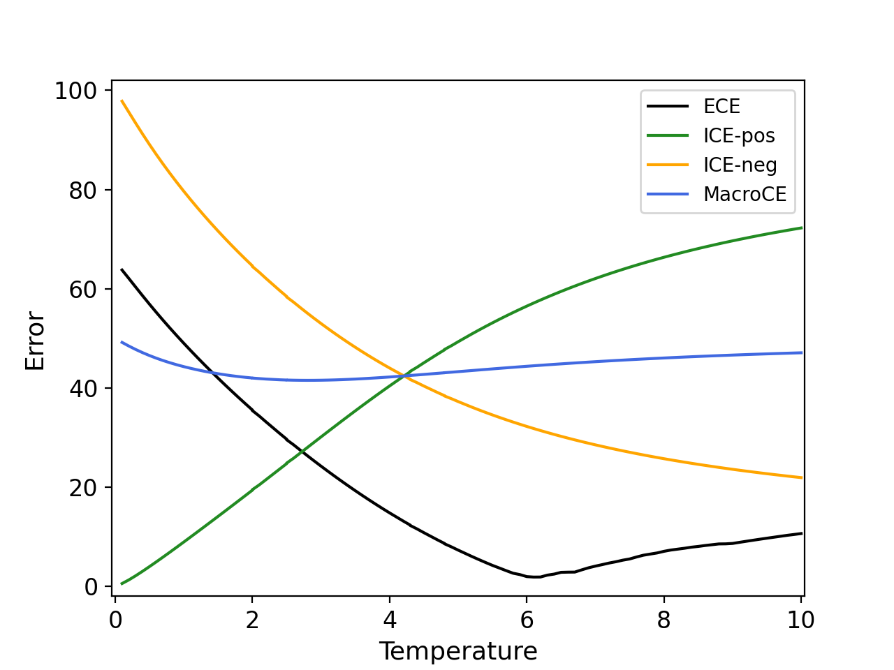
Figure 5: Calibration errors after temperature scaling. x-axis represents different temperature values; lines with different colors represent different metrics. MacroCE stays relatively constant while ece varies largely at different temperature values.

	IID (NQ)					OOD (HotpotQA)
Calibrator	EM	ECEinterval	ICEpos	ICEneg	MacroCE	EM	ECEinterval	ICEpos	ICEneg	MacroCE
No Calibration
Joint	35.24	30.41	27.17	61.74	44.46	24.50	44.40	25.38	67.04	46.21
Pipeline	36.34	50.08	6.93	82.63	44.78	22.78	61.22	12.48	82.95	47.72
Binary Baseline
Joint	35.24	38.03	53.22	29.77	41.50	24.50	38.62	55.81	33.05	44.43
Pipeline	36.34	33.68	46.34	26.46	36.40	22.78	38.82	55.45	33.92	44.68
Average Baseline
Joint	35.24	2.00	64.25	35.75	50.00	24.50	11.25	64.25	35.75	50.00
Pipeline	36.34	0.03	63.66	36.34	50.00	22.78	13.56	63.66	36.34	50.00
Temperature Scaling
Joint	35.24	4.69	53.98	31.08	42.53	24.50	13.72	55.17	36.07	45.62
Pipeline	36.34	5.49	58.57	30.54	44.55	22.78	8.14	65.78	29.95	47.86
Feature-based Classifier
Logistic Regression	37.26	61.50	0.04	98.04	49.04	21.37	76.56	0.46	97.39	48.93
SVM	36.51	52.30	4.88	85.18	45.03	21.82	62.40	10.93	82.87	46.90
Random Forest	36.40	47.41	9.57	80.02	44.79	24.61	53.88	16.78	76.95	46.87
Neural Reranker (ReConsider)
Softmax	37.62	33.83	33.70	62.24	50.47	26.54	46.80	27.84	69.79	48.81
Sigmoid	37.62	58.61	9.37	72.59	40.97	26.54	51.41	23.56	70.40	46.98
Label Smoothing
Joint	36.12	29.42	28.81	62.36	45.59	23.57	44.69	25.88	67.76	46.82
+ TS	36.12	5.57	56.41	30.48	43.45	23.57	14.31	56.27	35.82	46.04
Ensemble Calibration (Binary)
Joint	37.78	28.95	45.23	19.06	32.15	25.68	31.86	59.93	22.15	41.04
Pipeline	38.98	29.22	45.63	18.75	32.19	23.43	32.17	58.48	24.11	41.30
Ensemble Calibration (Frequency)
Joint	37.78	34.12	15.95	64.53	40.24	25.68	43.95	21.62	66.62	44.12
Pipeline	38.98	33.00	15.93	64.26	40.10	23.43	47.03	21.16	67.89	44.52
Consistency Calibration (Binary)
Joint	35.24	31.91	26.10	35.07	30.59	24.50	40.37	34.29	42.35	38.32
Pipeline	36.34	31.30	25.91	34.38	30.15	22.78	43.25	37.00	45.09	41.05
Consistency Calibration (Frequency)
Joint	35.24	44.46	26.39	44.68	35.53	24.50	46.21	31.72	49.89	40.81
Pipeline	36.34	44.78	26.04	43.78	34.91	22.78	47.72	32.34	51.87	42.11
Consistency Calibration (Classifier)
Joint	35.24	31.63	27.28	34.00	30.64	24.50	40.34	35.56	41.90	38.73
Pipeline	36.34	33.16	25.84	37.34	31.59	22.78	44.60	31.81	48.38	40.09

Table 7: Calibration results of baseline calibration methods as well as our new consistency calibration. We compare using the joint and pipeline approach for obtaining the top answer predictions. We highlight the best result in bold. Our new consistency calibration method outperforms all other baselines on MacroCE for both the joint and pipeline implementation. Note that different metrics give different ranking of these methods, which further highlights the importance of using a reliable and informative metric.

Appendix C Dataset Details

Natural Questions (NQ) (Kwiatkowski et al., 2019) consists of questions mined from Google search queries. We use the open version of NQ where each question has answers with up to five tokens found from Wikipedia (Lee et al., 2019). We use NQ for training and in-distribution evaluation.

SQuAD (Rajpurkar et al., 2016) contains a set of questions written by crowdworkers given a Wikipedia paragraph. We use the open version of SQuAD following Chen et al. (2017). We use SQuAD for out-of-distribution evaluation.

TriviaQA (Joshi et al., 2017) includes trivia questions scraped from the web. We use the unfiltered version for out-of-distribution evaluation.

HotpotQA (Yang et al., 2018) is a multi-hop question answering dataset written by crowdworkers given a pair of Wikipedia paragraphs. We take the full-wiki version of HotpotQA and use it for out-of-distribution evaluation.

Appendix D Additional Baselines and Variants

We compare two ways of obtaining the top prediction of each checkpoint - joint (considering top predictions from all top-10 retrieved passages) and pipeline (only considering the top predictions from top-1 retrieved passage). In the main paper (Table 2) we reported results of using the joint approach. We compare these two variants in Table 7.

We also explore two other alternative implementations of ConsCal. The first one is frequency-based ConsCal where the confidence of each prediction is computed as $\frac{k}{n}$ where $k$ is the number of times that the prediction was made by the $n$ total checkpoints. The second one is classifier-based ConsCal where we treat whether the final prediction is also predicted by each intermediate checkpoint as a binary feature, and train a linear classifier on such $n$-dimensional feature vectors ($n$ is the number of checkpoints used) to predict the correctness of the final prediction. We use the predicted probability from this classifier as the calibrated confidence value. These variants are compared in Table 7. Interestingly, the binary implementation of ConsCal turns out to be the most important than all other baselines and variants.

	IID (NQ)					OOD (HotpotQA)
Calibrator	EM	ECEinterval	ICEpos	ICEneg	MacroCE	EM	ECEinterval	ICEpos	ICEneg	MacroCE
Non-Consistency Baselines
No Calibration
Joint	35.24	30.41	27.17	61.74	44.46	24.50	44.40	25.38	67.04	46.21
Pipeline	36.34	50.08	6.93	82.63	44.78	22.78	61.22	12.48	82.95	47.72
Binary Baseline
Joint	35.24	38.03	53.22	29.77	41.50	24.50	38.62	55.81	33.05	44.43
Pipeline	36.34	33.68	46.34	26.46	36.40	22.78	38.82	55.45	33.92	44.68
Average Baseline
Joint	35.24	2.00	64.25	35.75	50.00	24.50	11.25	64.25	35.75	50.00
Pipeline	36.34	0.03	63.66	36.34	50.00	22.78	13.56	63.66	36.34	50.00
Consistency Calibration with n=17
Consistency Calibration (Binary)
Joint	35.24	31.91	26.10	35.07	30.59	24.50	40.37	34.29	42.35	38.32
Pipeline	36.34	31.30	25.91	34.38	30.15	22.78	43.25	37.00	45.09	41.05
Consistency Calibration (Frequency)
Joint	35.24	44.46	26.39	44.68	35.53	24.50	46.21	31.72	49.89	40.81
Pipeline	36.34	44.78	26.04	43.78	34.91	22.78	47.72	32.34	51.87	42.11
Consistency Calibration (Classifier)
Joint	35.24	31.63	27.28	34.00	30.64	24.50	40.34	35.56	41.90	38.73
Pipeline	36.34	33.16	25.84	37.34	31.59	22.78	44.60	31.81	48.38	40.09
Consistency Calibration with n=9
Consistency Calibration (Binary)
Joint	35.24	34.07	24.29	39.39	31.84	24.50	42.88	30.61	46.86	38.74
Pipeline	36.34	32.52	23.78	37.51	30.65	22.78	45.36	32.30	49.22	40.76
Consistency Calibration (Frequency)
Joint	35.24	23.17	25.06	46.05	35.56	24.50	33.91	30.34	51.29	40.81
Pipeline	36.34	21.84	24.94	44.71	34.83	22.78	35.93	30.80	52.98	41.89
Consistency Calibration (Classifier)
Joint	35.24	32.19	27.67	34.64	31.16	24.50	41.11	36.71	42.53	39.62
Pipeline	36.34	31.36	26.37	34.20	30.29	22.78	43.70	36.01	45.97	40.99
Consistency Calibration with n=5
Consistency Calibration (Binary)
Joint	35.24	33.07	26.02	37.43	31.72	24.50	41.33	34.41	43.58	38.99
Pipeline	36.34	32.49	26.30	36.03	31.16	22.78	43.67	36.51	47.02	41.77
Consistency Calibration (Frequency)
Joint	35.24	26.70	22.74	48.21	35.48	24.50	35.86	28.22	53.07	40.65
Pipeline	36.34	25.44	22.54	46.92	34.73	22.78	39.05	29.39	55.08	42.24
Consistency Calibration (Classifier)
Joint	35.24	33.41	26.02	37.43	31.72	24.50	41.33	34.41	43.58	38.99
Pipeline	36.34	31.16	31.78	30.81	31.30	22.78	40.43	43.31	39.58	41.45

Table 8: Results of using consistency calibration with a larger number of checkpoints ($n=\{9,17\}$). The difference with using $n=5$ is small. Note that $n$ represents the total number of checkpoints apart being used. We find that the impact of using different $n$ is small. We reported results of using $n=5$ in the main paper.

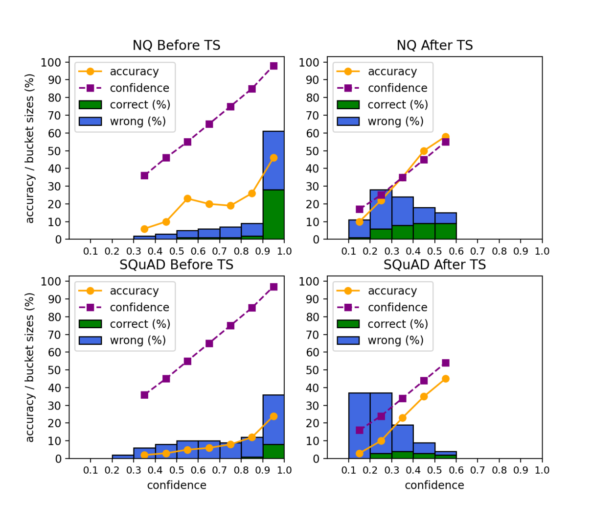
Figure 6: Bucketing distribution of predictions on nq and HotpotQA. The x-axis represents the confidence range of each bucket, the y-axis represents the average answer accuracy for the dashed line plot and represents the relative bucket sizes for the histogram. Similar flaws hold true for these two datasets: after temperature scaling, all predictions’ confidence values are scaled to become closer to the overall answer accuracy, and correct (green bars) and wrong predictions (blue bars) are mixed in the same buckets, making it hard to distinguish.

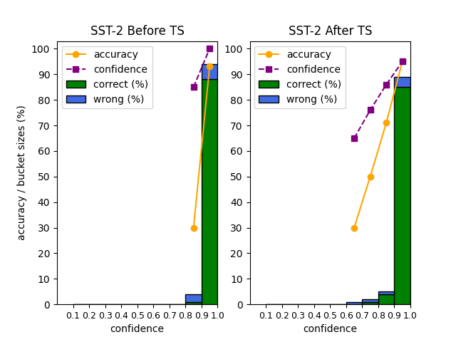
Figure 7: Bucketing distribution of predictions on SST-2 Socher et al. (2013), a binary sentiment analysis dataset. We can see the same trend as on nq and HotpotQA - all predictions’ confidence are very close. In fact, on SST-2, all predictions have high confidence both before and after temperature scaling, making it hard for users to identify wrong predictions.

Appendix E Impact of Checkpoint Numbers in ConsCal

In the main paper we saved a total number of $n=5$ checkpoints during training for ConsCal. In order to understand the impact of this hyper-parameter $n$, we experiment with $n=\{9,17\}$ and report the results in Table 8. We observe that the impact of different $n$ is very small.

Appendix F Illustration of ece Flaws on More Datasets

In the main paper we illustrated the flaws of ece with a case study on HotpotQA. Here we additional present visualizations of calibration results on nq (in-domain) and SQuAD (ood). As shown in Figure 6, the flaws of ece as described in the main paper hold true for these datasets as well, validating the generality of our conclusions.

In addition to qa, we also present results on a sentiment analysis dataset in Figure 7. We observe the same trends that all predictions have similar confidence scores, making it difficult to identify the wrong predictions.

References

- Brier (1950) Glenn W. Brier. 1950. Verification of forecasts expressed in terms of probability. Monthly Weather Review.
- Brown et al. (2020) Tom B. Brown, Benjamin Mann, Nick Ryder, Melanie Subbiah, Jared Kaplan, Prafulla Dhariwal, Arvind Neelakantan, Pranav Shyam, Girish Sastry, Amanda Askell, Sandhini Agarwal, Ariel Herbert-Voss, Gretchen Krueger, T. J. Henighan, Rewon Child, Aditya Ramesh, Daniel M. Ziegler, Jeff Wu, Clemens Winter, Christopher Hesse, Mark Chen, Eric Sigler, Mateusz Litwin, Scott Gray, Benjamin Chess, Jack Clark, Christopher Berner, Sam McCandlish, Alec Radford, Ilya Sutskever, and Dario Amodei. 2020. Language models are few-shot learners. In Proceedings of Advances in Neural Information Processing Systems.
- Chen et al. (2017) Danqi Chen, Adam Fisch, Jason Weston, and Antoine Bordes. 2017. Reading wikipedia to answer open-domain questions. In Proceedings of the Association for Computational Linguistics.
- Desai and Durrett (2020) Shrey Desai and Greg Durrett. 2020. Calibration of pre-trained transformers. In Proceedings of Empirical Methods in Natural Language Processing.
- Devlin et al. (2019) Jacob Devlin, Ming-Wei Chang, Kenton Lee, and Kristina Toutanova. 2019. BERT: Pre-training of deep bidirectional transformers for language understanding. In Proceedings of the Association for Computational Linguistics.
- Dhuliawala et al. (2022) Shehzaad Dhuliawala, Leonard Adolphs, Rajarshi Das, and Mrinmaya Sachan. 2022. Calibration of machine reading systems at scale. In Findings of the Association for Computational Linguistics: ACL.
- Guo et al. (2017) Chuan Guo, Geoff Pleiss, Yu Sun, and Kilian Q Weinberger. 2017. On calibration of modern neural networks. In Proceedings of the International Conference of Machine Learning.
- Iyer et al. (2021) Srini Iyer, Sewon Min, Yashar Mehdad, and Wen tau Yih. 2021. Reconsider: Re-ranking using span-focused cross-attention for open domain question answering. In Proceedings of the Association for Computational Linguistics.
- Jiang et al. (2021) Zhengbao Jiang, Jun Araki, Haibo Ding, and Graham Neubig. 2021. How can we know when language models know? on the calibration of language models for question answering. Transactions of the Association for Computational Linguistics.
- Joshi et al. (2017) Mandar Joshi, Eunsol Choi, Daniel Weld, and Luke Zettlemoyer. 2017. TriviaQA: A large scale distantly supervised challenge dataset for reading comprehension. In Proceedings of the Association for Computational Linguistics.
- Kamath et al. (2020) Amita Kamath, Robin Jia, and Percy Liang. 2020. Selective question answering under domain shift. In Proceedings of the Association for Computational Linguistics.
- Karpukhin et al. (2020) Vladimir Karpukhin, Barlas Oğuz, Sewon Min, Patrick Lewis, Ledell Wu, Sergey Edunov, Danqi Chen, and Wen-tau Yih. 2020. Dense passage retrieval for open-domain question answering. In Proceedings of Empirical Methods in Natural Language Processing.
- Kwiatkowski et al. (2019) Tom Kwiatkowski, Jennimaria Palomaki, Olivia Redfield, Michael Collins, Ankur Parikh, Chris Alberti, Danielle Epstein, Illia Polosukhin, Matthew Kelcey, Jacob Devlin, Kenton Lee, Kristina N. Toutanova, Llion Jones, Ming-Wei Chang, Andrew Dai, Jakob Uszkoreit, Quoc Le, and Slav Petrov. 2019. Natural questions: A benchmark for question answering research. Transactions of the Association for Computational Linguistics.
- Lee et al. (2019) Kenton Lee, Ming-Wei Chang, and Kristina Toutanova. 2019. Latent retrieval for weakly supervised open domain question answering. In Proceedings of the Association for Computational Linguistics.
- Lin et al. (2022) Stephanie C. Lin, Jacob Hilton, and Owain Evans. 2022. Truthfulqa: Measuring how models mimic human falsehoods. In Proceedings of Association for Computational Linguistics.
- Maynez et al. (2020) Joshua Maynez, Shashi Narayan, Bernd Bohnet, and Ryan T. McDonald. 2020. On faithfulness and factuality in abstractive summarization. In Proceedings of Association for Computational Linguistics.
- Minderer et al. (2021) Matthias Minderer, Josip Djolonga, Rob Romijnders, Frances Hubis, Xiaohua Zhai, Neil Houlsby, Dustin Tran, and Mario Lucic. 2021. Revisiting the calibration of modern neural networks. In Proceedings of Advances in Neural Information Processing Systems.
- Naeini et al. (2015) Mahdi Pakdaman Naeini, Gregory F. Cooper, and Milos Hauskrecht. 2015. Obtaining well calibrated probabilities using bayesian binning. In Association for the Advancement of Artificial Intelligence.
- Nguyen and O’Connor (2015) Khanh Nguyen and Brendan T. O’Connor. 2015. Posterior calibration and exploratory analysis for natural language processing models. In Proceedings of Empirical Methods in Natural Language Processing.
- Niculescu-Mizil and Caruana (2005) Alexandru Niculescu-Mizil and Rich Caruana. 2005. Predicting good probabilities with supervised learning. In Proceedings of the International Conference of Machine Learning.
- Nixon et al. (2019) Jeremy Nixon, Michael W Dusenberry, Linchuan Zhang, Ghassen Jerfel, and Dustin Tran. 2019. Measuring calibration in deep learning. In CVPR Workshops.
- Pereyra et al. (2017) Gabriel Pereyra, G. Tucker, Jan Chorowski, Lukasz Kaiser, and Geoffrey E. Hinton. 2017. Regularizing neural networks by penalizing confident output distributions. In Proceedings of the International Conference on Learning Representations.
- Rajpurkar et al. (2016) Pranav Rajpurkar, Jian Zhang, Konstantin Lopyrev, and Percy Liang. 2016. SQuAD: 100,000+ questions for machine comprehension of text. In Proceedings of Empirical Methods in Natural Language Processing.
- Rodriguez et al. (2019) Pedro Rodriguez, Shi Feng, Mohit Iyyer, He He, and Jordan L. Boyd-Graber. 2019. Quizbowl: The case for incremental question answering. ArXiv.
- Si et al. (2022) Chenglei Si, Zhe Gan, Zhengyuan Yang, Shuohang Wang, Jianfeng Wang, Jordan Boyd-Graber, and Lijuan Wang. 2022. Prompting gpt-3 to be reliable. arXiv, abs/2210.09150.
- Socher et al. (2013) Richard Socher, Alex Perelygin, Jean Wu, Jason Chuang, Christopher Manning, Andrew Ng, and Christopher Potts. 2013. Recursive deep models for semantic compositionality over a sentiment treebank. In Proceedings of Empirical Methods in Natural Language Processing.
- Swayamdipta et al. (2020) Swabha Swayamdipta, Roy Schwartz, Nicholas Lourie, Yizhong Wang, Hannaneh Hajishirzi, Noah A. Smith, and Yejin Choi. 2020. Dataset cartography: Mapping and diagnosing datasets with training dynamics. In Proceedings of Empirical Methods in Natural Language Processing.
- Thulasidasan et al. (2019) Sunil Thulasidasan, Gopinath Chennupati, Jeff A. Bilmes, Tanmoy Bhattacharya, and Sarah Ellen Michalak. 2019. On mixup training: Improved calibration and predictive uncertainty for deep neural networks. In Proceedings of Advances in Neural Information Processing Systems.
- Yang et al. (2018) Zhilin Yang, Peng Qi, Saizheng Zhang, Yoshua Bengio, William W Cohen, Ruslan Salakhutdinov, and Christopher D Manning. 2018. Hotpotqa: A dataset for diverse, explainable multi-hop question answering. In Proceedings of Empirical Methods in Natural Language Processing.
- Ye and Durrett (2022) Xi Ye and Greg Durrett. 2022. Can explanations be useful for calibrating black box models? In Proceedings of the Association for Computational Linguistics.
- Zhang et al. (2021) Shujian Zhang, Chengyue Gong, and Eunsol Choi. 2021. Knowing more about questions can help: Improving calibration in question answering. In Findings of the Association for Computational Linguistics: ACL.