Physics Guided Machine Learning for Variational Multiscale Reduced Order Modeling

Abstract

We propose a new physics guided machine learning (PGML) paradigm that leverages the variational multiscale (VMS) framework and available data to dramatically increase the accuracy of reduced order models (ROMs) at a modest computational cost. The hierarchical structure of the ROM basis and the VMS framework enable a natural separation of the resolved and unresolved ROM spatial scales. Modern PGML algorithms are used to construct novel models for the interaction among the resolved and unresolved ROM scales. Specifically, the new framework builds ROM operators that are closest to the true interaction terms in the VMS framework. Finally, machine learning is used to reduce the projection error and further increase the ROM accuracy. Our numerical experiments for a two-dimensional vorticity transport problem show that the novel PGML-VMS-ROM paradigm maintains the low computational cost of current ROMs, while significantly increasing the ROM accuracy.

Keywords Reduced order modeling, Variational multiscale method, Physics guided machine learning, Nonlinear proper orthogonal decomposition, Autoencoder, Galerkin projection

1 Introduction

The behavior of physical systems can be generally described by physical principles (e.g., conservation of mass, momentum, and energy) together with constitutive laws. The resulting models are often mathematically formulated as partial differential equations (PDEs) (e.g., the Navier-Stokes equations). Solving them allows prediction and analysis of the system’s dynamics. The applicability of analytic methods for solving PDEs is usually limited to simple cases with special geometry and under severe assumptions. In practice, numerical approaches (e.g., finite difference, finite volume, spectral, and finite element methods) are utilized to discretize the governing equations and approximate the values of the unknowns corresponding to a given grid. For turbulent flows, we need to deal with an exceedingly large number of degrees of freedom due to the existence of a wide range of spatio-temporal scales to be resolved. Although such models, called here full order models (FOMs), are capable of providing very accurate results, they can be computationally demanding. Therefore, FOMs become impractical for applications that require multiple forward evaluations with varying inputs (e.g., flow control [1, 2, 3], optimization [4, 5, 6, 7, 8, 9, 10], and digital twinning [11, 12, 13, 14, 15, 16]) or studies requiring several simulations like computational-aided clinical trials [17].

Reduced order models (ROMs) are defined as computationally light surrogates that can mimic the behavior of FOMs with sufficient accuracy [18, 19, 20, 21, 22]. Projection-based ROMs have gained significant popularity in the past few decades due to the increased amounts of collected data (either from actual experiments or numerical simulations) as well as the development of system identification tools [23, 24]. Of particular interest, the combination of proper orthogonal decomposition (POD) and Galerkin projection has been a powerful driver for ROM progress. The process comprises an offline stage and an online stage. The offline stage starts with the collection of data corresponding to system realizations (called snapshots) at different time instants and/or parameter values. With these data sets, POD provides a hierarchy of basis functions (or modes) that capture the maximum amount of the underlying system’s energy (defined by the data variance). The offline stage is concluded by performing a Galerkin projection of the FOM operators onto the subspace spanned by a truncated set of POD modes to obtain a system of ordinary differential equations (ODEs) representing the Galerkin ROM (GROM). Although this offline stage can be extremely expensive, the resulting GROM can be utilized during the online deployment phase to efficiently predict the system’s behavior at parameter values and/or time instants different from those in the data preparation process.

The GROM framework has been successful in many applications (e.g., [25, 26, 27, 28, 29, 30, 31, 32, 22]), especially those dominated by diffusion mechanisms or periodic dynamics. Those are often referred to as systems with a solution manifold that is characterized by a small Kolmogorov $n$-width [33, 34]. In the POD context, this means that the dynamics can be accurately represented by a few modes. However, for convection-dominated flows with strong nonlinearity, the Kolmogorov $n$-width is often large with a slow decay, which hinders the linear reducibility of the underlying system.

The repercussions of a Galerkin truncation and projection are two-fold. First, the span of the retained POD basis functions does not necessarily provide an accurate representation of the solution and it gives rise to the projection error [35, 36, 37]. Second, the interactions between the truncated and the retained modes can be significant. These interactions are ignored in the Galerkin projection step, and consequently the GROM cannot in general capture the dynamics of the resolved modes accurately. This introduces a closure error [38, 39, 40, 41, 42, 43, 44, 45, 46, 47, 48]. Several efforts have been devoted to address the closure problem. A recent survey covering a plethora of physics-based and data-driven ROM closure methodologies can be found in [22].

The closure problem has been historically related to the stabilization of the ROM solution, drawing roots from large eddy simulation (LES) studies, where the truncated small scales are thought of having diffusive effects on the larger scales. Therefore, eddy viscosity-based frameworks have been often used in the ROM literature [49]. Nonetheless, it was found that introducing eddy viscosity to all resolved scales can actually unnecessarily contaminate the dynamics of the largest scales. To mitigate this problem, the variational multiscale (VMS) method, which was proposed by Hughes’ group [50, 51, 52] in the finite element setting (see, e.g., [53, 54] for a survey), was utilized to add eddy viscosity dissipation to only a portion of the ROM resolved scales in [55, 56, 38]. A data-driven version of VMS (DD-VMS) has been recently proposed in [57], where the effects of the truncated modes onto the GROM dynamics are not restricted to be diffusive.

In the present study, we transform the DD-VMS [57, 58] and provide an alternative modular framework by utilizing machine learning (ML) capabilities. We stress that this is a fundamental change in which the standard DD-VMS regression is replaced by ML in order to better account for closure effects. Therefore, the proposed neural network approach is essentially different from the regression based DD-VMS [57]. In particular, the DD-VMS ansatz of a quadratic polynomial closure model is relieved by utilizing the deep neural network (DNN) functionality with memory embedding. We also leverage the long short-term memory (LSTM) variant of recurrent neural networks (RNNs) to approximate scale-aware closures. In essence, the use of LSTM encompasses a non-Markovian closure, supported by the Mori-Zwanzig formalism [59, 60, 61, 62, 63]. Moreover, we adopt the physics guided machine learning (PGML) framework introduced in [64, 65, 66] to reduce the uncertainty of the output results. In particular, we exploit concatenation layers informed by the VMS-ROM arguments to enrich the neural network architecture and constrain the learning algorithm to the manifold of physically-consistent solutions. Finally, for problems with a large Kolmogorov $n$-width, we utilize the nonlinear POD (NLPOD) methodology [67] to reduce the projection error without affecting the computational efficiency, by learning the correlations among the small unresolved scales to provide much fewer latent space variables. We also perform a numerical investigation of the proposed strategies (ML-VMS-ROM, PGML-VMS-ROM, and NLPOD-VMS-ROM), with a particular focus on the locality of scale interactions, which is a cornerstone of the VMS framework.

The rest of the paper is organized as follows: We briefly describe the reduced order modeling methodology by the nexus of POD and Galerkin projection in Section 2. The relevant background information and notations for the VMS approach are given in Section 3. The use of the PGML methodology to provide reliable predictions is explained in Section 4, while the NLPOD approach is discussed in Section 5. The proposed NLPOD-PGML-VMS framework is tested for the parametric unsteady vortex-merger problem, which exemplifies convection-dominated flow systems. Results and discussions are presented in Section 6, followed by the concluding remarks in Section 7.

2 Reduced Order Modeling

A Newtonian incompressible fluid flow in a domain $\Omega\subset\mathbb{R}^{d}$, where $d$ defines the spatial dimension (i.e., $d\in\{2,3\})$, can be described by the Navier-Stokes equations (NSE). In order to eliminate the pressure term, we consider the NSE in the vorticity-vector potential formulation. In particular, we consider the 2D case where the vector potential is reduced to the streamfunction as follows:

$$\partial_{t}\omega-\nu\Delta\omega+(\boldsymbol{u}\cdot\nabla)\omega =0,\qquad\text{in}\ \Omega\times[0,T],$$ (1)

$$\Delta\psi+\omega =0,\qquad\text{in}\ \Omega\times[0,T],$$

where $\omega(\boldsymbol{x},t)$ and $\psi(\boldsymbol{x},t)$ denote the vorticity and streamfunction fields, respectively, for $\boldsymbol{x}\in\Omega$ and $t\in[0,T]$, while $\nu$ stands for the kinematic viscosity (diffusion coefficient). In dimensionless form, $\nu$ represents the reciprocal of the Reynolds number, Re. The velocity vector field $\boldsymbol{u}(\boldsymbol{x},t)$ is related to the streamfunction as follows:

$$\boldsymbol{u}=\nabla^{\perp}\psi,\quad\nabla^{\perp}=[\partial_{y},-\partial_{x}]^{T}.$$ (2)

By using Eq. (2), Eq. Eq. 1 can be further rewritten as follows:

$$\partial_{t}\omega-\nu\Delta\omega+J(\omega,\psi) =0,\qquad\text{in}\ \Omega\times[0,T],$$ (3)

where $J(\cdot,\cdot)$ denotes the Jacobian operator, which is defined as follows:

$$J(\omega,\psi)=\dfrac{\partial\omega}{\partial x}\dfrac{\partial\psi}{\partial y}-\dfrac{\partial\omega}{\partial y}\dfrac{\partial\psi}{\partial x}.$$ (4)

The vorticity transport equation (Eq. Eq. 3) is equipped with an initial condition and boundary conditions on $\Gamma:=\partial\Omega$. For convenience and simplicity of presentation, we shall assume the following conditions:

$$IC: \ \omega(\boldsymbol{x},0)=\omega_{0}(\boldsymbol{x}), \text{in}\ \Omega,$$ (5)

$$BC\ \mathrm{(non-slip)}: \ \psi(\boldsymbol{x},t)=0,\quad\dfrac{\partial\psi}{\partial\boldsymbol{n}}=0, \text{in}\ \Gamma\times[0,T].$$

In the remainder of this section, we describe the construction of the projection-based ROM of the vorticity transport equation. This includes the use of POD to approximate the solution (Section 2.1), followed by the Galerkin method, where the FOM operators in Eq. Eq. 1 are projected onto the POD subspace to define the sought GROM (Section 2.2).

2.1 Proper orthogonal decomposition

We consider a collection of system realizations defined by an ensemble of vorticity fields $\{\omega(\boldsymbol{x},t_{0}),\allowbreak\omega(\boldsymbol{x},t_{1}),\dots,\allowbreak\omega(\boldsymbol{x},t_{M-1})\}$. These are often called snapshots and come from either experimental measurements or numerical simulations of Eq. Eq. 1 or Eq. Eq. 3 using any of the standard discretization schemes (e.g., finite element, finite difference or finite volume methods). Without loss of generality, we assume that these snapshots are sampled at equidistant $M$ $(>1)$ time instants with $t_{m}=m\Delta t$, where $m=0,1,\dots,M-1$ and $\Delta t=\dfrac{T}{M-1}$. We note that, in general, these snapshots can correspond to different types of parameters (e.g., operating conditions, physical properties, and geometry).

In POD, we seek a low-dimensional basis $\{\phi_{1},\phi_{2},\dots,\phi_{R}\}$ that optimally approximates the space spanned by the snapshots in the following sense [49]:

$$\min\ \Bigg{\langle}\bigg{\|}\omega(\cdot,\cdot)-\sum_{k=1}^{R}\big{(}\omega(\cdot,\cdot),\phi_{k}(\cdot)\big{)}\phi_{k}(\cdot)\bigg{\|}^{2}\Bigg{\rangle},$$ (6)

$$\text{subject to}\qquad\quad\|\phi\|=1,\qquad\big{(}\phi_{i}(\cdot),\phi_{j}(\cdot)\big{)}=\delta_{ij},$$

where $\langle\cdot\rangle$ denotes an average operation with respect to the parametrization, $(\cdot,\cdot)$ is an inner product, and $\|\cdot\|$ is the corresponding norm. For example, an ensemble average based on temporal snapshots can be defined as follows:

$$\langle\omega\rangle=\dfrac{1}{M}\sum_{m=0}^{M-1}\omega(\cdot,t_{m}).$$ (7)

The snapshots represent the approximation of the quantity of interest on a specific grid. For example, a realization of the vorticity field at a given time can be arranged in a column vector $\boldsymbol{\omega}\in\mathbb{R}^{N}$, where $N$ is the number of grid points. It can be shown that solving the optimization problem Eq. 6 amounts to solving the following eigenvalue problem [68]:

$$\mathbf{D}\Phi=\Phi\Lambda,$$ (8)

where the entries of the diagonal matrix $\Lambda$ and the columns of $\Phi$ represent the eigenpairs of the spatial autocorrelation matrix $\mathbf{D}\in\mathbb{R}^{N\times N}$ with entries defined as

$$\big{[}\mathbf{D}\big{]}_{ij}=\bigg{\langle}\boldsymbol{\omega}(\boldsymbol{x}_{i},\cdot)\boldsymbol{\omega}(\boldsymbol{x}_{j},\cdot)\bigg{\rangle},$$ (9)

where $\boldsymbol{\omega}(\boldsymbol{x}_{i},\cdot)$ is the $i$-th entry of $\boldsymbol{\omega}$. For fluid flow problems, the length of the vector $\boldsymbol{\omega}$ is often large, which makes the eigenvalue problem in Eq. Eq. 8 computationally challenging.

Sirovich [69, 70, 71] proposed a numerical procedure, known as the method of snapshots, to reduce the computational cost of solving Eq. Eq. 8. This approach is efficient, especially when the number of collected snapshots $M$ is much smaller than the number of degrees of freedom (i.e., $M\ll N$), as it reduces the $N\times N$ eigenvalue problem in Eq. Eq. 8 to an $M\times M$ problem. The spatial autocorrelation matrix $\mathbf{D}\in\mathbb{R}^{N\times N}$ is replaced by the temporal snapshot correlation matrix $\mathbf{K}\in\mathbb{R}^{M\times M}$ with entries defined as follows:

$$\big{[}\mathbf{K}\big{]}_{ij}=\dfrac{1}{M}\bigg{(}\omega(\cdot,t_{i}),\omega(\cdot,t_{j})\bigg{)}.$$ (10)

The following eigenvalue problem is thus considered:

$$\mathbf{K}\mathbf{v}_{k}=\lambda_{k}\mathbf{v}_{k},$$ (11)

where $\mathbf{v}_{k}$ is the $k^{\text{th}}$ eigenvector of $\mathbf{K}$ and $\lambda_{k}$ is the associated eigenvalue. To obtain the hierarchy of the POD basis, the eigenpairs are sorted in a descending order by their eigenvalues (i.e., $\lambda_{1}\geq\lambda_{2}\dots\geq\lambda_{M}\geq 0$). Finally, the POD basis functions can be computed as a linear superposition of the collected snapshots as follows [68]:

$$\phi_{k}(\cdot)=\dfrac{1}{\sqrt{\lambda_{k}}}\sum_{m=0}^{M-1}[\mathbf{v}_{k}]_{m}\omega(\cdot,t_{m}),$$ (12)

where $[\mathbf{v}_{k}]_{m}$ denotes the $m^{\text{th}}$ component of $\mathbf{v}_{k}$. It can be verified that the basis functions in Eq. Eq. 12 are orthonormal (i.e., $(\phi_{i}(\cdot),\phi_{j}(\cdot))=\delta_{ij}$), where $\delta_{ij}$ is the Kronecker delta. The POD eigenvalues define the contribution of each mode toward the total variance in the given snapshots. A metric that evaluates the quality of a given set of retained modes in representing the system is the relative information content (RIC) [22], defined as follows:

$$\text{RIC}(k)=\dfrac{\sum_{l=1}^{k}\lambda_{l}}{\sum_{l=1}^{M}\lambda_{l}},$$ (13)

where $k$ is the POD index at which modal truncation takes place. We emphasize that the same approach can be applied considering parameters other than time. In this case, the temporal correlation matrix is substituted by a generalized parameter correlation matrix.

2.2 Galerkin projection

The GROM starts by the Galerkin truncation step, making use of the optimality criterion in Eq. Eq. 6 as follows:

$$\omega(\boldsymbol{x},t_{m})\approx\omega_{R}(\boldsymbol{x},t_{m})=\sum_{k=1}^{R}a_{k}(t_{m})\phi_{k}(\boldsymbol{x}),$$ (14)

where $\{a_{k}\}_{k=1}^{R}$ are the time-varying modal coefficients (weights), known as generalized coordinates. The optimal values of these coefficients are defined by the true projection of the FOM trajectory onto the corresponding POD basis function as follows:

$$a_{k}(t_{m})=\big{(}\omega(\cdot,t_{m}),\phi_{k}(\cdot)\big{)}.$$ (15)

Next, the vorticity field $\omega$ in Eq. Eq. 3 is replaced by its approximation $\omega_{R}$ from Eq. Eq. 14. After this, the Galerkin projection step comes into play, by defining the POD test subspace $\boldsymbol{X}_{R}$ as follows:

$$\boldsymbol{X}_{R}:=\text{span}\{\phi_{1},\phi_{2},\dots,\phi_{R}\}.$$ (16)

Finally, Eq. Eq. 3 with $\omega$ replaced by $\omega_{R}$ is projected onto the POD space $\boldsymbol{X}_{R}$. This yields the GROM of the vorticity transport equation: Find $\omega_{R}\in\boldsymbol{X}_{R}$ such that:

$$(\partial_{t}\omega,\phi)-\nu(\Delta\omega,\phi)+\big{(}J(\omega,\psi),\phi\big{)} =0,\qquad\forall\phi\in\boldsymbol{X}_{R}.$$ (17)

Equation Eq. 17 can be written in a tensorial form as follows:

$$\dot{\boldsymbol{a}}=A\boldsymbol{a}+\boldsymbol{a}^{\top}B\boldsymbol{a},$$ (18)

where $\boldsymbol{a}(t)\in\mathbb{R}^{R}$ is the vector of unknown coefficients $\{a_{k}\}_{k=1}^{R}$, while $A\in\mathbb{R}^{R\times R}$ and $B\in\mathbb{R}^{R\times R\times R}$ are the matrix and tensor corresponding to the linear and nonlinear terms, respectively.

The Galerkin truncation step restricts the approximation of the vorticity field to live in a low-rank subspace $\boldsymbol{X}_{R}$ ($R\ll N$), which might not capture all the relevant flow structures. Therefore, a projection error is introduced. Furthermore, the Galerkin projection step enforces the dynamics of the ROM to be defined using only the scales supported by $\boldsymbol{X}_{R}$. Nonetheless, due to the coupling between different modes, the unresolved scales (i.e., the scales modeled by $\{\phi_{k}\}_{k\geq R+1}$) influence the dynamics of the resolved scales (i.e., the scales modeled by $\{\phi_{k}\}_{k\leq R}$). By neglecting these mutual interactions, the GROM becomes incapable of accurately describing the dynamics of the retained modes, which is usually referred to as the closure problem [22].

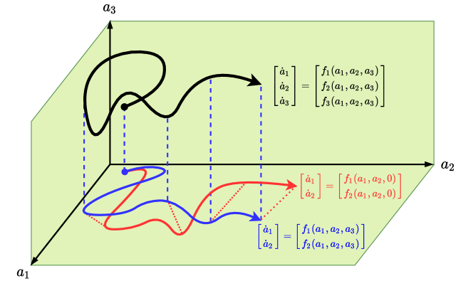
Figure 1: Representation of the repercussions of modal truncation onto the ROM solution. The solid black curve denotes the FOM trajectory, assuming that the full rank expansion is defined by $a_{1}$, $a_{2}$, and $a_{3}$. The solid blue curve defines the projection of the FOM trajectory onto a two-dimensional subspace. The vertical dashed blue lines refer to the projection or representation error. Note that evaluating $a_{1}$ and $a_{2}$ still requires the knowledge of the FOM trajectory (i.e.,$a_{1}$, $a_{2}$, and $a_{3}$) at every point. In practice, we only have information regarding the resolved variables (i.e., $a_{1}$ and $a_{2}$), so the contribution of $a_{3}$ towards the dynamics of $a_{1}$ and $a_{2}$ is neglected. This yields a closure error, denoted by the dashed red lines.

The projection error and closure error are illustrated in Fig. 1, for a toy system whose full-rank approximation can be represented with 3 modes as follows:

$$\omega(x,t)=a_{1}(t)\phi_{1}(x)+a_{2}(t)\phi_{2}(x)+a_{3}(t)\phi_{3}(x).$$ (19)

Assuming that the FOM is written in the following form:

$$\dot{\omega}=F(\omega),$$ (20)

then the dynamics of $\{a_{k}\}_{k=1}^{3}$ can be described as $\dot{a}_{k}=(F(\omega),\phi_{k})$. Thus, the FOM trajectory can be written as follows:

$$\begin{bmatrix}\dot{a}_{1}\\ \dot{a}_{2}\\ \dot{a}_{3}\end{bmatrix}=\begin{bmatrix}f_{1}(a_{1},a_{2},a_{3})\\ f_{2}(a_{1},a_{2},a_{3})\\ f_{3}(a_{1},a_{2},a_{3})\end{bmatrix}.$$ (21)

In other words, evolving $\{a_{k}\}_{k=1}^{3}$ using Eq. Eq. 21 and reconstructing $\omega$ with Eq. Eq. 19 recovers the FOM field (equivalent to solving Eq. Eq. 20 using standard discretization schemes). For the sake of demonstration, we suppose that we retain only 2 modes in the ROM approximation. This corresponds to removing the third row in Eq. Eq. 21 as follows:

$$\begin{bmatrix}\dot{a}_{1}\\ \dot{a}_{2}\end{bmatrix}=\begin{bmatrix}f_{1}(a_{1},a_{2},a_{3})\\ f_{2}(a_{1},a_{2},a_{3})\end{bmatrix}.$$ (22)

Approximating $\omega$ with just two modes results in losing the flow structures that are contained in the truncated mode (the vertical direction in Fig. 1), which yields the projection error. Furthermore, we note that $f_{1}$ and $f_{2}$ are usually functions of $a_{1}$, $a_{2}$, and $a_{3}$ for systems with strong nonlinearity and coupling between different modes. However, during ROM deployment, we do not usually have information regarding the unresolved dynamics ($a_{3}$ in this example). Thus, in GROM, the effects of the truncated scales onto the resolved scales are assumed to be negligible, as follows:

$$\begin{bmatrix}\dot{a}_{1}\\ \dot{a}_{2}\end{bmatrix}=\begin{bmatrix}f_{1}(a_{1},a_{2},0)\\ f_{2}(a_{1},a_{2},0)\end{bmatrix}.$$ (23)

We denote the reference trajectory described by Eq. Eq. 22 as the true projection, which is related to Eq. Eq. 15. This defines the best low-rank approximation that can be obtained for a given number of modes, assuming we have access to the whole set of FOM scales. The difference between the GROM trajectory (corresponding to solving Eq. Eq. 23) and the true projection trajectory represents the closure error. In the present study, we address both the closure error and the projection error. First, to tackle the closure problem, we leverage the VMS framework outlined in Section 3 to develop the PGML methodology in Section 4. Then, we utilize the NLPOD approach in Section 5 to reduce the projection error by learning a compressed latent space that encapsulates some of the truncated flow structures.

3 Variational Multiscale Method

The variational multiscale (VMS) methods are general numerical discretizations that significantly increase the accuracy of classical Galerkin approximations in under-resolved simulations, e.g., on coarse meshes or when not enough basis functions are available. The VMS framework, which was proposed by Hughes and coworkers [50, 51, 52], has made a profound impact in many areas of computational mechanics (see, e.g., [53, 54] for a survey).

To illustrate the standard VMS methodology, we consider a general nonlinear partial differential equation

$$\dot{\omega}=F(\omega),$$ (24)

whose weak (variational) form is

$$(\dot{\omega},\phi)=(F(\omega),\phi),\quad\forall\phi\in\boldsymbol{X},$$ (25)

where $F$ is a general nonlinear function and $\boldsymbol{X}$ is an appropriate test space. To build the VMS framework, we start with a sequence of hierarchical spaces of increasing resolutions: $\boldsymbol{X}_{1}$, $\boldsymbol{X}_{1}\oplus\boldsymbol{X}_{2}$, $\boldsymbol{X}_{1}\oplus\boldsymbol{X}_{2}\oplus\boldsymbol{X}_{3}$, $\dots$. Next, we project system Eq. 24 onto each of the spaces $\boldsymbol{X}_{1}$, $\boldsymbol{X}_{2}$, $\boldsymbol{X}_{3}$, $\dots$, which yields a separate equation for each space. From a computational efficiency point of view, the goal is to solve for the $\omega$ component that lives in the coarsest space (i.e., $\boldsymbol{X}_{1}$), since this yields the lowest-dimensional system:

$$(\dot{\omega},\phi)=(F(\omega),\phi),\quad\forall\phi\in\boldsymbol{X}_{1}.$$ (26)

However, system Eq. 26 is not closed since its right-hand side involves $\omega$ components that do not belong to $\boldsymbol{X}_{1}$ (i.e., $\omega_{2}\in\boldsymbol{X}_{2}$, $\omega_{3}\in\boldsymbol{X}_{3}$, $\dots$):

$$(F(\omega),\phi)=(F(\omega_{1},\omega_{2},\omega_{3},\dots),\phi),\quad\forall\phi\in\boldsymbol{X}_{1}.$$ (27)

Thus, the VMS closure problem needs to be solved. That is, Eq. Eq. 27 needs to be replaced with an equation that involves only terms that belong to $\boldsymbol{X}_{1}$. In general, the VMS system in Eq. Eq. 26 equipped with an appropriate closure model (i.e., a model with components in $\boldsymbol{X}_{1}$ that captures the interaction between $\omega_{1}$ and the scales in $\boldsymbol{X}_{2},\boldsymbol{X}_{3},\ldots$) yields an accurate approximation of the $\boldsymbol{X}_{1}$ component of $\omega$.

The POD procedure in Section 2.1 yields a hierarchy of orthogonal basis functions, sorted by their contribution to the total energy. Therefore, it provides a natural fit to the VMS framework. Next, we illustrate the adoption of VMS in GROM settings to define a multi-level VMS ROM. In particular, we detail the two-scale and the three-scale VMS ROMs, while further extensions become straightforward.

3.1 Two-scale VMS ROM

The two-scale VMS (VMS-2) ROM utilizes two orthogonal spaces, $\boldsymbol{X}_{1}$ and $\boldsymbol{X}_{2}$, defined as follows:

$$\boldsymbol{X}_{1} :=\text{span}\{\phi_{1},\phi_{2},\dots,\phi_{R}\},$$ (28)

$$\boldsymbol{X}_{2} :=\text{span}\{\phi_{R+1},\phi_{R+2},\dots,\phi_{N}\},$$

where $\boldsymbol{X}_{1}$ represents the span of the resolved ROM scales and $\boldsymbol{X}_{2}$ is the span of the unresolved scales. Thus, $\omega$ can be written as follows:

$$\omega=\sum_{k=1}^{R}a_{k}\phi_{k}+\sum_{k=R+1}^{N}a_{k}\phi_{k}=\underbrace{\omega_{R}}_{\text{resolved}}+\underbrace{\omega^{\prime}}_{\text{unresolved}},$$ (29)

where $\omega_{R}\in\boldsymbol{X}_{1}$ is the resolved ROM component of $\omega$, while $\omega^{\prime}\in\boldsymbol{X}_{2}$ is the unresolved component. Using this decomposition, Eq. Eq. 26 can be rewritten as follows:

$$\big{(}\dot{\omega}_{R},\phi_{k}\big{)}=\big{(}F(\omega_{R}),\phi_{k}\big{)}+\underbrace{\bigg{[}\big{(}F(\omega),\phi_{k}\big{)}-\big{(}F(\omega_{R}),\phi_{k}\big{)}\bigg{]}}_{\text{VMS-2 closure term}},\ \forall k\in\{1,\dots,R\}.$$ (30)

The bracketed term in Eq. Eq. 30 is the VMS-2 closure term, which models the interaction between the ROM modes and the discarded modes. Since the unresolved component of $\omega$, $\omega^{\prime}$, is not available during online deployment stage, it is not possible to exactly compute the closure term in practical settings. Instead, the closure term can be approximated using a generic function $G(\omega_{R})$ as follows:

$$\big{(}G(\omega_{R}),\phi_{k})\approx\big{(}F(\omega),\phi_{k}\big{)}-\big{(}F(\omega_{R}),\phi_{k}\big{)},$$ (31)

and the VMS-2 ROM can be written as

$$\big{(}\dot{\omega}_{R},\phi_{k}\big{)}=\big{(}F(\omega_{R}),\phi_{k}\big{)}+\big{(}G(\omega_{R}),\phi_{k}).$$ (32)

The form and parameters of $G$ will be defined in Section 4.

3.2 Three-scale VMS ROM

The locality of modal interactions is a cornerstone of the VMS framework. It states that neighboring modes have more mutual interactions than those who are far apart in the energy spectrum. For this reason, it is natural to distinguish between neighboring and far modes when closure modeling is performed. To this end, the flexibility of the hierarchical structure of the ROM space is leveraged to perform a three-scale decomposition of $\omega$, leading to a three-scale VMS (VMS-3) ROM, which aims at increasing the VMS-2 ROM accuracy. To construct the VMS-3 ROM, we first build three orthogonal spaces, $\boldsymbol{X}_{1}$, $\boldsymbol{X}_{2}$, and $\boldsymbol{X}_{3}$, as follows:

$$\boldsymbol{X}_{1} :=\text{span}\{\phi_{1},\phi_{2},\dots,\phi_{r}\},$$ (33)

$$\boldsymbol{X}_{2} :=\text{span}\{\phi_{r+1},\phi_{r+2},\dots,\phi_{R}\},$$

$$\boldsymbol{X}_{3} :=\text{span}\{\phi_{R+1},\phi_{R+2},\dots,\phi_{N}\}.$$

Compared to the decomposition into resolved and unresolved scales in Section 3.1, $\boldsymbol{X}_{1}$ now represents the large resolved ROM scales, $\boldsymbol{X}_{2}$ represents the small resolved ROM scales, while $\boldsymbol{X}_{3}$ denotes the unresolved ROM scales. With these definitions, $\omega$ can be written as follows:

$$\omega =\sum_{k=1}^{r}a_{k}\phi_{k}+\sum_{k=r+1}^{R}a_{k}\phi_{k}+\sum_{k=R+1}^{N}a_{k}\phi_{k}$$ (34)

$$=\underbrace{\omega_{L}}_{\text{large resolved}}+\underbrace{\omega_{S}}_{\text{small resolved}}+\underbrace{\omega^{\prime}}_{\text{unresolved}}.$$

This is similar to Eq. Eq. 29 with $\omega_{R}=\omega_{L}+\omega_{S}$. To construct the VMS-3 ROM, we project system Eq. 24 onto each of the spaces $\boldsymbol{X}_{1}$ and $\boldsymbol{X}_{2}$, as follows:

$$\big{(}\dot{\omega}_{L},\phi_{k}\big{)}=\big{(}F(\omega_{L}+\omega_{S}),\phi_{k}\big{)}+\bigg{[}\big{(}F(\omega),\phi_{k}\big{)}-\big{(}F(\omega_{L}+\omega_{S}),\phi_{k}\big{)}\bigg{]},\ k=1,\ldots,r,$$ (35)

$$\big{(}\dot{\omega}_{S},\phi_{k}\big{)}=\big{(}F(\omega_{L}+\omega_{S}),\phi_{k}\big{)}+\bigg{[}\big{(}F(\omega),\phi_{k}\big{)}-\big{(}F(\omega_{L}+\omega_{S}),\phi_{k}\big{)}\bigg{]},\ k=r+1,\ldots,R.$$ (36)

Although the two bracketed terms in Eq. Eq. 35 and Eq. Eq. 36 defining the VMS-3 closure terms look similar, they have different roles. The first term models basically the interaction between the large and the small resolved modes, because the interaction large-unresolved is assumed to be negligible (according to the VMS principle of locality of modal interactions). The second term models the interaction between the small resolved and the unresolved ROM modes. This allows great flexibility in choosing the structure of the different VMS ROM closure terms. This concept is investigated numerically in Section 6.

4 Physics Guided Machine Learning

In this section, the VMS-2 and VMS-3 closure terms defined in Section 3 are approximated using only the information in the resolved scales. Specifically, we utilize a purely data-driven approach to compute the parameters of the closure models. However, instead of relying on heuristics or ad-hoc arguments to define the specific structure of the closure model (as in the standard DD-VMS [57]), we exploit the capabilities of deep neural network (DNN) in approximating arbitrary functions. In particular, we use the long short-term memory (LSTM) variant of recurrent neural networks (RNNs), which has shown substantial success in data-driven modeling of time series [72, 73, 74]. We emphasize that, to mitigate well-known drawbacks of data-driven modeling (e.g., sensitivity to noise in input data), the VMS ROM framework utilizes data to model only the VMS ROM closure operators, but all the other ROM operators are built by using classical Galerkin projection. Thus, our VMS ROM framework incorporates “data-driven closure,” rather than “data-driven modeling” for the resolved scales.

4.1 ML-VMS ROM

The VMS-2 ROM in Eq. Eq. 32 can be rewritten as follows:

$$\dot{\boldsymbol{a}}=\boldsymbol{f}(\boldsymbol{a})+\boldsymbol{c}(\boldsymbol{a}),$$ (37)

where $\boldsymbol{a}=[a_{1},a_{2},\dots,a_{R}]^{T}\in\mathbb{R}^{R}$ is the vector of coefficients for resolved POD modes, $\boldsymbol{f}(\boldsymbol{a})=[\big{(}F(\omega_{R}),\phi_{1}\big{)},\big{(}F(\omega_{R}),\phi_{2}\big{)},\dots,\big{(}F(\omega_{R}),\phi_{R}\big{)}]$ represents the Galerkin projection of the FOM operators onto the POD subspace, and $\boldsymbol{c}(\boldsymbol{a})=[c_{1},c_{2},\dots,c_{R}]^{R}\in\mathbb{R}^{R}$ is the vector of the closure (correction) terms, i.e., $c_{k}=(G(\omega_{R}),\phi_{k})$. In the present study, we use DNN to represent the closure model, i.e., $\boldsymbol{c}(\cdot)\approx\pi_{\theta}(\boldsymbol{a})$, where $\theta$ denotes the parameterization of the LSTM. The general functional form of the DNN models used for temporal forecasting can be written as follows:

$$\mathbf{h}^{(n)} =f_{h}^{h}(\boldsymbol{a}^{(n)},\mathbf{h}^{(n-1)}),$$ (38)

$$\boldsymbol{c}^{(n)} =f_{h}^{o}(\mathbf{h}^{(n)}),$$

where $\boldsymbol{a}^{(n)}:=\boldsymbol{a}(t_{n})\in\mathbb{R}^{R}$ is the vector of modal coefficients at time $t_{n}$ and $\boldsymbol{c}^{(n)}\in\mathbb{R}^{R}$ is the corresponding closure term, defining the input and output of the DNN, respectively. In Eq. Eq. 38, $\mathbf{h}\in\mathbb{R}^{H}$ represents the hidden-state of the neural network, $f_{h}^{h}$ and $f_{h}^{o}$ the hidden-to-hidden and hidden-to-output mappings, respectively, and $H$ the dimension of the hidden state. The Mori-Zwanzig formulation [75, 76, 77, 44, 78] shows that non-Markovian terms are required to account for the effects of the unresolved scales onto the resolved scales. Thus, the closure operators are modeled as functions of the time history of the resolved scales. We emphasize that employing a non-Markovian closure model is a key feature of the proposed PGML-VMS-ROM that is in stark contrast with the DD-VMS in [57, 58], which considers only the Markovian effects.

For memory embedding, we let $\boldsymbol{c}$ be a function of the short time history of the resolved POD coefficients, i.e., $\boldsymbol{c}^{(n)}(\cdot)\approx\pi_{\theta}(\boldsymbol{a}^{(n)},\boldsymbol{a}^{(n-1)},\dots,\boldsymbol{a}^{(n-\tau)})=\pi_{\theta}(\boldsymbol{a}^{(n):(n-\tau)})$, where $\tau$ defines the length of the time history of $\boldsymbol{a}$ that is required for estimating the closure term. The LSTM allows modeling non-Markovian processes while mitigating the issue with vanishing (or exploding) gradient by employing gating mechanisms. In particular, the hidden-to-hidden mapping $f_{h}^{h}$ is defined using the following equations:

$$\mathbf{g}_{f}^{(n)} =\sigma_{f}(\mathbf{W}_{f}[\mathbf{h}^{(n-1)},\boldsymbol{a}^{(n)}]+\mathbf{b}_{f}),$$ (39)

$$\mathbf{g}_{i}^{(n)} =\sigma_{i}(\mathbf{W}_{i}[\mathbf{h}^{(n-1)},\boldsymbol{a}^{(n)}]+\mathbf{b}_{i}),$$

$$\tilde{\mathbf{s}}^{(n)} =\tanh{(\mathbf{W}_{s}[\mathbf{h}^{(n-1)},\boldsymbol{a}^{(n)}]+\mathbf{b}_{s})},$$

$$\mathbf{s}^{(n)} =\mathbf{g}_{f}^{(n)}\odot\mathbf{s}^{(n-1)}+\mathbf{g}_{i}^{(n)}\odot\tilde{\mathbf{s}}^{(n)},$$

$$\mathbf{g}_{o}^{(n)} =\sigma_{o}(\mathbf{W}_{o}[\mathbf{h}^{(n-1)},\boldsymbol{a}^{(n)}]+\mathbf{b}_{o}),$$

$$\mathbf{h}^{(n)} =\mathbf{g}_{o}^{(n)}\odot\tanh{(\mathbf{s}^{(n)})},$$

where $\mathbf{g}_{f},\mathbf{g}_{i},\mathbf{g}_{o}\in\mathbb{R}^{H}$ are the forget gate, input gate, and output gate, respectively, with the corresponding $\mathbf{W}_{f},\mathbf{W}_{i},\mathbf{W}_{o}\in\mathbb{R}^{H\times(H+R)}$ weight matrices, and $\mathbf{b}_{f},\mathbf{b}_{i},\mathbf{b}_{o}\in\mathbb{R}^{H}$ bias vectors. $\mathbf{s}\in\mathbb{R}^{H}$ is the cell state with a weight matrix $\mathbf{W}_{s}\in\mathbb{R}^{H\times(H+R)}$ and bias vector $\mathbf{b}_{s}\in\mathbb{R}^{H}$. Finally, $\sigma$ is the sigmoid activation function, and $\odot$ denotes the element-wise multiplication.

We stack $l$ LSTM layers to define the hidden states, followed by a fully connected layer with a linear activation function to represent the hidden-to-output mapping. Thus, the ML-VMS-2 closure model can be written as

$$\boldsymbol{c}^{(n)}\approx\mathcal{L}(\cdot)\circ\mathbf{h}_{l}^{(n)}(\cdot)\circ\mathbf{h}_{l-1}^{(n):(n-\tau)}(\cdot)\circ\dots\circ\mathbf{h}_{1}^{(n):(n-\tau)}(\cdot)\circ\mathcal{I}(\boldsymbol{a}^{(n):(n-\tau)}),$$ (40)

where $\mathcal{L}(\cdot)$ represents the output layer with linear activation, and $\mathcal{I}(\cdot)$ denotes the input layer. Note that each of the internal LSTM layers ($i=1,2,\dots,l-1$) produces a sequence of hidden states $\mathbf{h}_{i}^{(n):(n-\tau)}$, while the the $l^{th}$ layer passes only the hidden state at the final time $\mathbf{h}_{l}^{(n)}$ to the output layer.

To summarize, Eqs. (37), (38), (39), and (40) yield the ML-VMS-2 ROM. In order to make use of the locality of modal interactions, the VMS-3 ROM is written as

$$\begin{bmatrix}\dot{\boldsymbol{a}_{L}}\\ \dot{\boldsymbol{a}_{S}}\end{bmatrix}=\boldsymbol{f}(\boldsymbol{a})+\begin{bmatrix}\boldsymbol{c}_{L}(\boldsymbol{a})\\ \boldsymbol{c}_{S}(\boldsymbol{a})\end{bmatrix},$$ (41)

where two separate terms are dedicated to model the closure for the resolved large scales and resolved small scales. For the ML-VMS-3, the closure terms are defined as follows:

$$\boldsymbol{c}^{(n)}_{L} \approx\pi_{L,\theta}(\boldsymbol{a}^{(n):(n-\tau)})$$ (42)

$$\approx\mathcal{L}_{{}_{L}}(\cdot)\circ\mathbf{h}_{l_{L}}^{(n)}(\cdot)\circ\mathbf{h}_{l-1_{L}}^{(n):(n-\tau)}(\cdot)\circ\dots\circ\mathbf{h}_{1_{L}}^{(n):(n-\tau)}(\cdot)\circ\mathcal{I}(\boldsymbol{a}^{(n):(n-\tau)}),$$

$$\boldsymbol{c}^{(n)}_{S} \approx\pi_{S,\theta}(\boldsymbol{a}^{(n):(n-\tau)})$$

$$\approx\mathcal{L}_{{}_{S}}(\cdot)\circ\mathbf{h}_{l_{S}}^{(n)}(\cdot)\circ\mathbf{h}_{l-1_{S}}^{(n):(n-\tau)}(\cdot)\circ\dots\circ\mathbf{h}_{1_{S}}^{(n):(n-\tau)}(\cdot)\circ\mathcal{I}(\boldsymbol{a}^{(n):(n-\tau)}).$$

We note that we have more flexibility in ML-VMS-3 than in ML-VMS-2. Hence, it is possible to make richer descriptions of the interactions between large resolved, small resolved, and unresolved scales.

4.2 PGML-VMS ROM

Critical aspects that should be considered during the adoption of ML based approach include their reliability, robustness, and trustworthiness. Previous studies [64, 65, 66] have reported high levels of uncertainty in the predictions of vanilla-type ML methods, especially for sparse data and incomplete governing equations regimes. In order to mitigate this issue, we utilize the physics-guided machine learning (PGML) paradigm to incorporate known physical arguments and constraints into the learning process. In particular, we exploit a modular approach to modify the neural network architectures through layer concatenation to inject physical information at different points in the latent space of the given DNN. This adaptation augments the performance during both the training and the deployment phases, and results in significant reduction in the uncertainty levels of the model prediction, as we demonstrate in Section 6.

In the PGML framework, the features extracted from the physics-based model are embedded into the generic $i^{th}$ intermediate hidden layer along with the latent variables. In order to build the PGML-VMS framework, we consider the Galerkin projection of the governing equations onto different POD modes to define the physics-based features (since they are derived from physical principles). Thus, the PGML-VMS-2 closure model can be written as

$$\boldsymbol{c}^{(n)}\approx\mathcal{L}(\cdot)\circ\mathbf{h}_{l}^{(n)}(\cdot) \circ\dots\circ\mathcal{C}\bigg{(}\mathbf{h}_{i}^{(n):(n-\tau)}(\cdot),\boldsymbol{f}^{(n):(n-\tau)}\bigg{)}\circ\mathbf{h}_{i-1}^{(n):(n-\tau)}(\cdot)\circ\dots\circ\mathbf{h}_{1}^{(n):(n-\tau)}(\cdot)\circ\mathcal{I}(\boldsymbol{a}^{(n):(n-\tau)}),$$ (43)

where $\mathcal{C}(\cdot,\cdot)$ represents the concatenation operation, and $\boldsymbol{f}^{(n):(n-\tau)}$ is the time history of projecting the FOM operators onto the truncated POD subspace. We highlight that there is no significant computational load for the calculation of $\boldsymbol{f}:=A\boldsymbol{a}+\boldsymbol{a}^{\top}B\boldsymbol{a}$, since $A$ and $B$ are already precomputed.

A schematic illustration of the PGML adaptation of the standard LSTM architecture is depicted in Fig. 2. In this figure, 3 LSTM layers are used (i.e., $l=3$), followed by a dense layer to provide the mapping from hidden state to the closure terms. The physics-based features are injected into the LSTM latent space after two hidden layers. One of the main advantages of the novel PGML framework in Fig. 2 is its modularity and simplicity. For example, based on the level of fidelity and our confidence in the injected features, we can promptly change the layer at which we embed them.

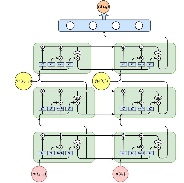
Figure 2: Illustration of the PGML methodology with concatenated LSTM layers. In this figure, a time history of $2$ time steps is used while physics-based features (yellow circles in the figure) are injected into the LSTM latent space after the second hidden layer ($i=2$).

Finally, the PGML-VMS-3 closure models can be written as

$$\boldsymbol{c}^{(n)}_{L}\approx\mathcal{L}_{{}_{L}}(\cdot)\circ\mathbf{h}_{l_{L}}^{(n)}(\cdot) \circ\dots\circ\mathcal{C}\bigg{(}\mathbf{h}_{i_{L}}^{(n):(n-\tau)}(\cdot),\boldsymbol{f}_{{}_{L}}^{(n):(n-\tau)}\bigg{)}\circ\mathbf{h}_{i-1_{L}}^{(n):(n-\tau)}(\cdot)\circ\dots\circ\mathbf{h}_{1_{L}}^{(n):(n-\tau)}(\cdot)\circ\mathcal{I}(\boldsymbol{a}^{(n):(n-\tau)}),$$ (44)

$$\boldsymbol{c}^{(n)}_{S}\approx\mathcal{L}_{{}_{S}}(\cdot)\circ\mathbf{h}_{l_{S}}^{(n)}(\cdot) \circ\dots\circ\mathcal{C}\bigg{(}\mathbf{h}_{i_{S}}^{(n):(n-\tau)}(\cdot),\boldsymbol{f}_{{}_{S}}^{(n):(n-\tau)}\bigg{)}\circ\mathbf{h}_{i-1_{S}}^{(n):(n-\tau)}(\cdot)\circ\dots\circ\mathbf{h}_{1_{S}}^{(n):(n-\tau)}(\cdot)\circ\mathcal{I}(\boldsymbol{a}^{(n):(n-\tau)}).$$

Note that in Eq. Eq. 44, we enjoy higher flexibility in choosing the physics-based features injected for each of the large and small scale closure models. For instance, in the present study, we benefit from the locality of modal interactions by embedding the Galerkin propagator of only a few relevant neighboring modes (i.e., $\boldsymbol{f}_{{}_{L}}$ and $\boldsymbol{f}_{{}_{S}}$ in Eq. 44), rather than including all of them in the LSTM learning (i.e., $\boldsymbol{f}$ in Eq. 43).

5 Nonlinear POD

In Section 3 and Section 4, we addressed the closure problem. That is, we aimed at correcting the ROM equations for the dynamics of the resolved scales including the effects of the unresolved scales onto the dynamics of the resolved scales. However, the reconstructed flow fields were approximated within the span of the retained modes, as shown in Eq. Eq. 14. Nonetheless, for turbulent flows the important flow structures generally span a large number of modes. Thus, truncating the solution beyond a small number of modes results in a large projection error. In other words, the component $\omega^{\prime}=\sum_{k=R+1}^{N}a_{k}\phi_{k}$ that cannot be approximated by the resolved POD basis becomes significant. In this section, we adapt the nonlinear POD (NLPOD) framework, introduced in [67], to model the unresolved part of the field. Fig. 3 presents a schematic representation of the PGML-VMS-3 model for the large and small resolved scales combined with NLPOD for enhanced field reconstruction. Note that, although both the PGML-VMS-3 and the NLPOD aim at increasing the ROM accuracy, they target different error sources: the PGML-VMS-3 aims at mitigating the closure error, whereas the NLPOD aims at alleviating the projection error.

The NLPOD methodology is based on combining POD with autoencoder (AE) techniques from ML to learn a latent representation of the POD expansion. It leverages the predefined hierarchy of POD basis functions, which satisfy the conservation laws and physical constraints, together with the capabilities of DNN to reveal the nonlinear correlations between the modes. Rather than using the NLPOD for the compression of the total set of POD coefficients, we constrain it to learn a few latent variables, which represent only the unresolved scales. To construct the NLPOD, we first define $\boldsymbol{b}=\{a_{k}\}_{k=R+1}^{K}$ corresponding to an almost full-rank POD expansion, where $K\leq N$ can be defined using the RIC spectrum (e.g., $\text{RIC}(K)\geq 99.99\%$). The goal is to learn $\boldsymbol{z}=\{z_{k}\}_{k=1}^{q}$, where $q\ll K$ denotes the dimension of the AE latent space.

The AE starts with an encoding process that involves applying a series of nonlinear mappings onto the input data to shrink the dimensionality down to a bottleneck layer representing the low rank or latent space embedding. An inverse mapping from the latent space variables to the same input is performed by another set of nonlinear mappings, defining the decoding part. For the NLPOD, the encoder and decoder can be represented as follows:

$$\text{Encoder}\ \eta :\boldsymbol{b}\in\mathbb{R}^{K-R}\mapsto\boldsymbol{z}\in\mathbb{R}^{q},\qquad\text{Decoder}\ \zeta :\boldsymbol{z}\in\mathbb{R}^{q}\mapsto\boldsymbol{b}\in\mathbb{R}^{K-R},$$ (45)

and they are trained jointly to minimize the following objective function:

$$\mathcal{J}=\sum_{n=1}^{N_{train}}\|\boldsymbol{b}^{(n)}-(\eta\circ\zeta)(\boldsymbol{b}^{(n)})\|,$$ (46)

where $N_{train}$ is the number of training samples.

In order to temporally propagate $\boldsymbol{z}$, we can use any of the regression tools, including sparse regression, Gaussian process regression, Seq2seq algorithms, temporal fusion transformers, and auto-regression methods. In the present study, we use LSTM architectures that are similar to the ones used in Section 4 to learn the one time-step mapping from $\boldsymbol{z}^{(n)}$ to $\boldsymbol{z}^{(n+1)}$, as follows:

$$\boldsymbol{z}^{(n+1)}\approx\mathcal{L}(\cdot)\circ\mathbf{h}_{l}^{(n)}(\cdot)\circ\mathbf{h}_{l-1}^{(n):(n-\tau)}(\cdot)\circ\dots\circ\mathbf{h}_{1}^{(n):(n-\tau)}(\cdot)\circ\mathcal{I}(\boldsymbol{z}^{(n):(n-\tau)}).$$ (47)

Note that the number of layers, $l$, and the length of time history, $\tau$, are not necessarily equal to those in Section 4. Moreover, the LSTM and AE can be trained either jointly or separately. In the present study, we train them separately for the sake of simplicity and to facilitate the NLPOD combination with other time series prediction tools.

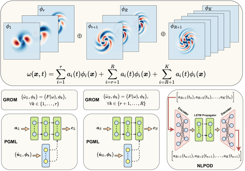
Figure 3: Schematic representation of the PGML-VMS-3 model for the large and small resolved scales, combined with NLPOD for enhanced field reconstruction. We note that PGML-VMS-3 is built upon a GROM for the first $R$ modes and mitigates the closure error (i.e., the effect of the truncated scales onto the resolved scales). In a complementary fashion, NLPOD implements an equation-free model for the truncated scales to reduce the projection error (i.e., the effect of the truncated scales onto the flow field reconstruction).

6 Results and Discussion

In this section, we perform a numerical investigation of the proposed PGML-VMS-ROM methodologies (with and without the NLPOD extension) using the two dimensional (2D) vortex merger problem [79], governed by the following vorticity transport equation:

$$\partial_{t}\omega+J(\omega,\psi)=\dfrac{1}{\text{Re}}\Delta\omega,\qquad\text{in}\ \Omega\times[0,T].$$ (48)

We consider a spatial domain of dimensions $(2\pi\times 2\pi)$ with periodic boundary conditions. The flow is initialized with a pair of co-rotating Gaussian vortices with equal strengths centered at $(x_{1},y_{1})=(5\pi/4,\pi)$ and $(x_{2},y_{2})=(3\pi/4,\pi)$ as follows:

$$\omega(x,y,0)=\exp\left(-\rho\left[(x-x_{1})^{2}+(y-y_{1})^{2}\right]\right)+\exp{\left(-\rho\left[(x-x_{2})^{2}+(y-y_{2})^{2}\right]\right)},$$ (49)

where $\rho$ is a parameter that controls the mutual interactions between the two vortical motions, set at $\rho=\pi$ in the present study. For the FOM simulations, we consider a regular Cartesian grid resolution of $256\times 256$ (i.e., $\Delta x=\Delta y=2\pi/256$), with a time-step of $0.001$. Vorticity snapshots are collected every 100 time-steps for $t\in[0,30]$, totalling 300 snapshots. The evolution of the vortex merger problem at selected values of the Reynolds number is depicted in Fig. 4, which illustrates the convective and interactive mechanisms affecting the transport and development of the two vortices.

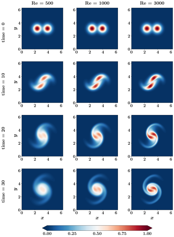
Figure 4: Samples of temporal snapshots of the vorticity field for the vortex merger problem at different values of Reynolds number.

In terms of POD analysis, we use $R=6$ to define the total number of resolved scales. For the three-scale VMS investigation, we split the resolved modes into 2 resolved large scales (i.e., $r=2$) and 4 resolved small scales. For the NLPOD study, we find that $K=20$ corresponds to near full-rank approximation of the flow field at all values of the Reynolds number. This is illustrated by the plot of the RIC values as a function of the number of POD modes at $\text{Re}=3000$ in Fig. 5.

Following a systematic approach, in Section 6.1, we first present our computational results for ML-VMS-2 and PGML-VMS-2 to quantitatively demonstrate the benefit of incorporating the physics guided machine learning approach. We then present the results for PGML-VMS-3 to highlight the flexibility and accuracy gain of the three-scale approach. Finally, in Section 6.2, we reveal the additional role of the NLPOD approach by illustrating the performance of the PGML-VMS-3+NLPOD approach.

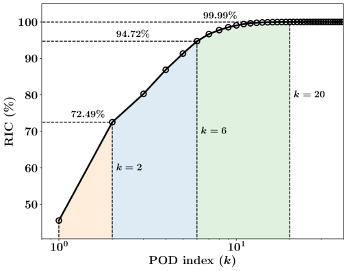
Figure 5: RIC values as a function of the modal truncation for the vortex merger problem at $\text{Re}=3000$.

6.1 Multi-level VMS closure for resolved scales

We store data corresponding to $\text{Re}\in\{500,750,1000,\dots,3000\}$ (in increments of 250), but we use only the data collected at $\text{Re}\in\{500,750,1000\}$ for neural network training, while the remaining data is reserved for testing purposes. First, we explore the combination of multi-level variational multiscale methods with machine learning. Fig. 6 displays the results of applying the ML-VMS-2 framework to model the closure term at $\text{Re}=3000$. In particular, we run a group of 10 LSTMs with different initializations of the neural network weights and utilize the deep ensemble method to quantify the uncertainty in the predictions. On the average, the ML-VMS-2 method provides accurate results compared to the GROM results. However, the uncertainty levels, described by the standard deviation in the ensemble predictions, are high. This is especially evident at the late time instants as the uncertainty propagates and grows with time.

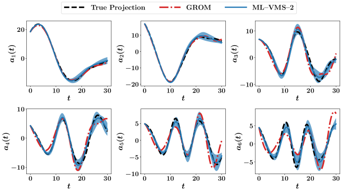
Figure 6: The time evolution of the first 6 modes of the vortex merger problem with the two-level VMS using ML closure, compared to the true projection and GROM (without closure) predictions. The solid line represents the mean values ($\mu$) from an ensemble of 10 different LSTM neural networks trained with different weight initalizations, while the shaded area defines the uncertainty bounds using standard deviation ($\sigma$) values. For better visualization, the shaded band is plotted with $\mu\pm 5\sigma$.

In order to increase the closure model robustness and reduce the uncertainty levels, we apply the PGML to inject physics-based features, as detailed in Section 4. Fig. 7 shows the evolution of the first 6 POD modal coefficients using the PGML-VMS-2. We can observe a significant reduction in the uncertainty levels as depicted by the shaded area, compared to the ML-VMS-2. It is also clear that the GROM yields inaccurate predictions. Moreover, we can observe that the deviations of the GROM trajectory from the true projections are larger for the latest resolved modes. In fact, this observation also applies to the ML-VMS-2 and PGML-VMS-2, which provide better results for the first two or three modes than the remaining ones.

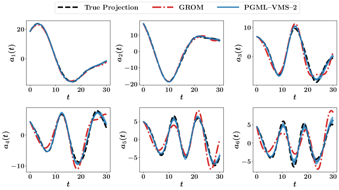
Figure 7: The time evolution of the first 6 modes of the vortex merger problem with the two-level VMS using PGML closure, compared to the true projection and GROM (without closure) predictions. The solid line represents the mean values ($\mu$) from an ensemble of 10 different LSTM neural networks trained with different weight initalizations, while the shaded area defines the uncertainty bounds using standard deviation ($\sigma$) values. For better visualization, the shaded band is plotted with $\mu\pm 5\sigma$.

In Fig. 8, we plot the ROM propagator $\dot{\boldsymbol{a}}$ computed by the Galerkin method (i.e., with truncation, with no access to the unresolved scales, and without correction) against the true propagator (assuming access to all the flow scales). We find that the GROM equations can adequately describe the dynamics of the first modes, but fail to do so for the last ones. This can be explained by locality of information transfer, which is one of the main concepts used in the VMS development. Such locality indicates that the neighboring modes exhibit larger mutual interactions than the modes which are far apart. Thus, describing the dynamics of the leading modes requires more information from the first few scales than from the remaining scales. In other words, the resolved scales become almost sufficient to define the propagator of the leading modes. On the other hand, the last modes are adjacent to the unresolved scales.Thus, the mode truncation considerably affects the dynamics of the last modes.

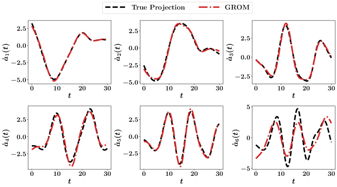
Figure 8: Comparison between the ROM propagator computed by Galerkin projection (with truncation, i.e., $\dot{a_{k}}=(-J(\omega_{R},\psi_{R})+\nabla^{2}\omega_{R},\phi_{k}$), against the true (FOM projection) propagator (i.e., $\dot{a_{k}}=(-J(\omega,\psi)+\nabla^{2}\omega,\phi_{k}$) at $\text{Re}=3000$, and $R=6$. We notice that the Galerkin projection accurately captures the dynamics of the first modes, but a discrepancy appears at the latest modes, which motivates the use of multi-level VMS closure.

In order to improve the quality of the closure model, we leverage the locality of modal interactions and apply the three-level VMS closure to correct the ROM dynamics. In particular, we split the resolved scales into two parts: the first 2 modes represent the largest resolved scales, while the remaining 4 modes represent the small resolved scales. The ML-VMS-3 predictions of the temporal dynamics for the first 6 modes are shown in Fig. 9. Compared to Fig. 6, the ML-VMS-3 provides more accurate results than the ML-VMS-2, even in terms of uncertainty levels.

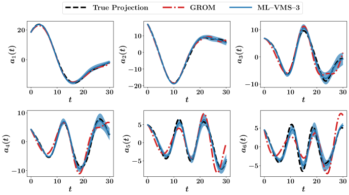
Figure 9: The time evolution of the first 6 modes of the vortex merger problem with the three-level VMS using ML closure, compared to the true projection and GROM (without closure) predictions. The solid line represents the mean values ($\mu$) from an ensemble of 10 different LSTM neural networks trained with different weight initalizations, while the shaded area defines the uncertainty bounds using standard deviation ($\sigma$) values. For better visualization, the shaded band is plotted with $\mu\pm 5\sigma$.

Finally, the PGML-VMS-3 results are shown in Fig. 10, where we can see improved results across all the resolved scales with very low levels of uncertainty. The mean squared error (MSE) between the true projection values of the resolved scales and the prediction of the ROM with and without various closure models is shown in Fig. 11. We can see that the VMS closure provides at least one order of magnitude better predictions than the baseline GROM. Moreover, the PGML-VMS is superior to the ML-VMS, especially for Reynolds number values that are not included in the LSTM training. This can be attributed to the fact that PGML employs physics-based features derived from the governing equations, resulting in improved extrapolatory capabilities of the overall model. Finally, the three-level variant of VMS is providing more accurate ROMs than VMS-2, making use of the locality of information transfer to build more localized closure models.

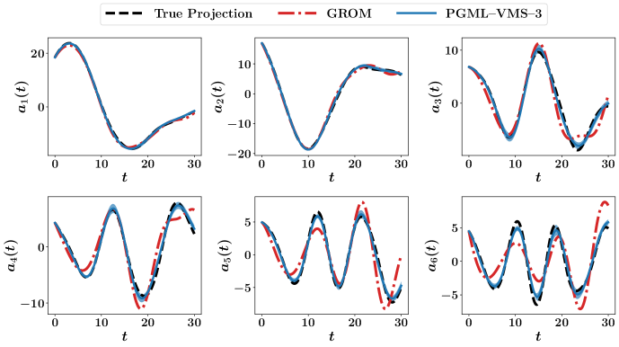
Figure 10: The time evolution of the first 6 modes of the vortex merger problem with the three-level VMS using PGML closure, compared to the true projection and GROM (without closure) predictions. The solid line represents the mean values ($\mu$) from an ensemble of 10 different LSTM neural networks trained with different weight initalizations, while the shaded area defines the uncertainty bounds using standard deviation ($\sigma$) values. For better visualization, the shaded band is plotted with $\mu\pm 5\sigma$.

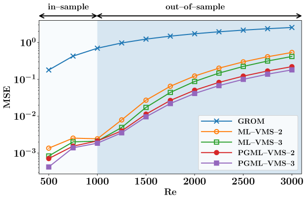
Figure 11: Mean squared error (MSE) between the true values of modal coefficients and the predictions of GROM, ML-VMS-2, ML-VMS-3, PGML-VMS-2, and PGML-VMS-3.

6.2 NLPOD for unresolved scales

The reconstructed vorticity fields from GROM, true projection, and PGML-VMS-3 at final time (i.e., $t=30$) at $\text{Re}=3000$ are visualized in Fig. 12. We can see that the GROM field is significantly inaccurate. In contrast, the PGML-VMS-3 is very close to the true projection field. This suggests that the PGML-VMS-3 is successful in providing accurate closure terms in such a way that the resulting ROM trajectory converges to the best linear approximation with 6 modes. Nonetheless, compared to the FOM solution, it is clear that 6 POD modes are not enough to capture all the relevant flow structures, especially at large values of the Reynolds number. On the other hand, building a projection-based ROM with increased number of modes will result in an undesired higher computational burden. In order to cure this limitation, we apply the NLPOD methodology from Section 5 to learn a latent space representation of important unresolved scales. We find that the value $K=20$ corresponds to $\text{RIC}\geq 99.99\%$, so we consider $\boldsymbol{b}=\{a_{k}\}_{k=7}^{20}\in\mathbb{R}^{14}$ in the NLPOD extension. We use the NLPOD to learn a two-dimensional compression of the resolved scales, i.e., $\boldsymbol{z}=\{z_{k}\}_{k=1}^{2}\in\mathbb{R}^{2}$. Fig. 13 displays the reconstructed vorticity fields at the final time from the true projection of the FOM field onto the first 6 and the first 20 POD modes. We notice that the FOM flow scales can be adequately captured by the subspace spanned by the first 20 POD modes. Furthermore, the plots clearly show that the combination of PGML-VMS-3 for the first 6 modes and NLPOD for the subsequent 14 modes (i.e., a total of 20 modes) provides improved field reconstruction. We highlight that the computational overhead of the online deployment of the PGML-VMS closure and NLPOD is negligible compared to solving the projection-based ROM with 6 modes.

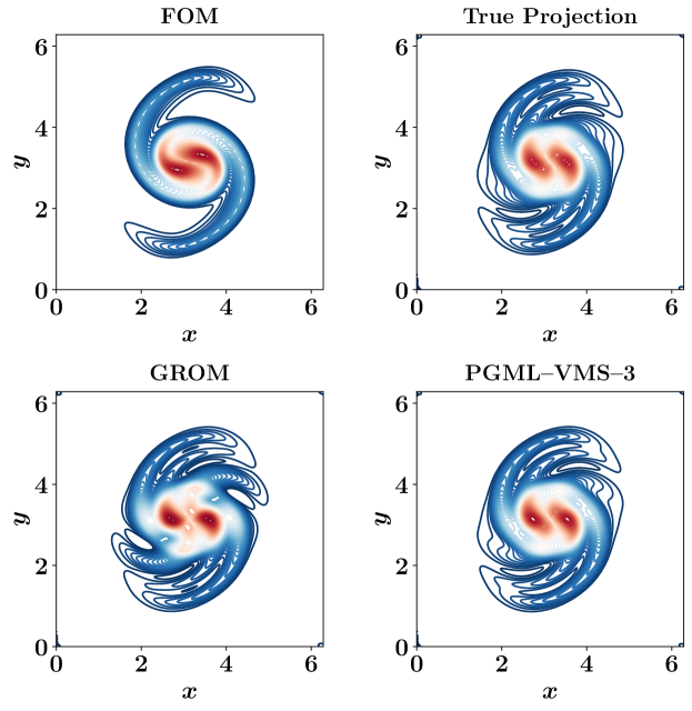
Figure 12: Comparison between the FOM vorticity field at the final time (i.e., $t=30$) and the reconstruction from true projection (i.e., optimal reconstruction), GROM, and PGML-VMS-3. Note that the PGML-VMS-3 field is very similar to the true projection field, which implies that the closure error is minimized. However, there are clear differences between the FOM and PGML-VMS-3 results, which suggest a significant projection error in the PGML-VMS-3 model.

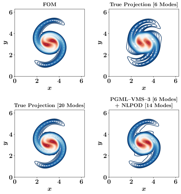
Figure 13: Comparison between the FOM vorticity field at final time (i.e., $t=30$) and the reconstruction from true projection (i.e., optimal reconstruction) at two different values of modal truncation, as well as the predictions of the PGML-VMS-3 for the dynamics of the first 6 modes, augmented with NLPOD for the following 14 modes (i.e., a total of $K=20$ modes) to reduce the projection error.

The CPU times for different portions of the FOM and ROMs are listed in Table 1. For the ROMs, we can see that the majority of the time is spent to train the neural networks during the offline stage. We note that this time can be significantly reduced by considering parallel training algorithms that make use of distributed hardware facilities. We also notice that the three-level VMS framework takes about twice the time taken by the two-level VMS due to the use of two distinct neural networks, which doubles the training and testing time. Nonetheless, we see that considerable computational gains are achieved compared to the FOM, by offloading most of the expensive computations to the offline stage resulting in computationally light models that can be used efficiently in the online stage. Moreover, we notice that the costs of the ML and PGML frameworks are of the same order, which implies that incorporating physics-based features into the neural network latent space comes with negligible overheads.

Table 1: Comparison of the CPU times for the offline and online stages for FOM and ROMs. Note that the PGML-VMS-3+NLPOD model yields a level of accuracy which is similar to the GROM ($R=20$) model with only a fraction of computational overhead (i.e., with a total computational online execution time of 63.876 s for the PGML-VMS-3+NLPOD model).

Offline CPU Time [s]		Online CPU Time [s]
POD Basis	0.646	FOM	1860.056
GROM Operators	0.246	GROM ($R=6$)	20.226
ML-VMS-2 Training	71.641	ML-VMS-2 ($R=6$)	32.289
ML-VMS-3 Training	148.057	ML-VMS-3 ($R=6$)	45.055
PGML-VMS-2 Training	65.324	PGML-VMS-2 ($R=6$)	33.358
PGML-VMS-3 Training	139.863	PGML-VMS-3 ($R=6$)	51.545
NLPOD Training (AE)	111.543	NLPOD ($R=6,K=20$)	12.331
NLPOD Training (LSTM)	85.234	GROM ($R=20$)	604.427

7 Conclusions and Future Work

We propose a hybrid hierarchical learning approach for the reduced order modeling of nonlinear fluid flow systems. The core component of the proposed method comprises a multi-level variational multiscale (VMS) framework for the natural separation of the resolved modes of different length scales and unresolved modes. We develop a modular physics-guided machine learning (PGML) paradigm through the concatenation of neural network layers to enable the convergence of the ROM trajectory of resolved scales to the optimal low-rank approximation. We use the projection of the governing equations onto the POD modes as physics-based features to constrain the output to a manifold of the physically realizable solutions. For a vorticity transport problem with high Reynolds numbers, we numerically demonstrate that this injection of physical information yields more robust and reliable ROM closures with reduced uncertainty levels. Moreover, we showcase the benefits of exploiting the locality of information transfer by building a three-level VMS, which centers around the scale-separation of the resolved modes into large resolved scales and small resolved scales. The numerical results show that the VMS-3 provides significant flexibility in defining the closure terms and is superior to the classical VMS-2 model used in previous studies. Finally, to decrease the projection error, we adapt the nonlinear proper orthogonal decomposition approach to learn a latent space representation of the unresolved ROM scales that yield a near-full rank approximation of the flow field.

Further investigations are required to optimize the layer(s) at which physics-based features are injected in the PGML framework. For example, we can add the injection at multiple points in the latent space, rather than a single point. Moreover, we may fuse various information from different models by repeating the concatenation operator for each piece of information. It is worth noting that advanced hyperparameter tuning approaches for the automated design of neural network architectures (e.g., using genetic algorithms) can be utilized to find the optimal layer(s) to inject the physics in the PGML architectures. In the present study, the ML-VMS, PGML-VMS, and NLPOD components of the hybrid framework are treated separately. In other words, the training of each neural network takes place independently of other neural networks in the framework. In a follow-up study, we plan to explore the simultaneous training of these neural networks to ensure that these models are integrated seamlessly in the computational workflow. Finally, the truncated scales that are recovered by NLPOD can be further embedded in the PGML-VMS architecture to improve the approximation of the closure model.

References

- [1] Bernd R Noack, Marek Morzynski, and Gilead Tadmor. Reduced-order modelling for flow control, volume 528. Springer Science & Business Media, New Yorok, 2011.
- [2] Kazufumi Ito and Sivaguru S Ravindran. A reduced-order method for simulation and control of fluid flows. Journal of Computational Physics, 143(2):403–425, 1998.
- [3] SS Ravindran. Reduced-order adaptive controllers for fluid flows using POD. Journal of Scientific Computing, 15(4):457–478, 2000.
- [4] Yi-dong Lang, Adam Malacina, Lorenz T Biegler, Sorin Munteanu, Jens I Madsen, and Stephen E Zitney. Reduced order model based on principal component analysis for process simulation and optimization. Energy & Fuels, 23(3):1695–1706, 2009.
- [5] Matthew J Zahr and Charbel Farhat. Progressive construction of a parametric reduced-order model for PDE-constrained optimization. International Journal for Numerical Methods in Engineering, 102(5):1111–1135, 2015.
- [6] Joris Degroote, Jan Vierendeels, and Karen Willcox. Interpolation among reduced-order matrices to obtain parameterized models for design, optimization and probabilistic analysis. International Journal for Numerical Methods in Fluids, 63(2):207–230, 2010.
- [7] David Amsallem, Matthew Zahr, Youngsoo Choi, and Charbel Farhat. Design optimization using hyper-reduced-order models. Structural and Multidisciplinary Optimization, 51(4):919–940, 2015.
- [8] Peter Benner, Ekkehard Sachs, and Stefan Volkwein. Model order reduction for PDE constrained optimization. Trends in PDE constrained optimization, pages 303–326, 2014.
- [9] Tan Bui-Thanh, Karen Willcox, Omar Ghattas, and Bart van Bloemen Waanders. Goal-oriented, model-constrained optimization for reduction of large-scale systems. Journal of Computational Physics, 224(2):880–896, 2007.
- [10] Benjamin Peherstorfer, Karen Willcox, and Max Gunzburger. Survey of multifidelity methods in uncertainty propagation, inference, and optimization. Siam Review, 60(3):550–591, 2018.
- [11] Adil Rasheed, Omer San, and Trond Kvamsdal. Digital twin: Values, challenges and enablers from a modeling perspective. IEEE Access, 8:21980–22012, 2020.
- [12] Michael G Kapteyn, Jacob VR Pretorius, and Karen E Willcox. A probabilistic graphical model foundation for enabling predictive digital twins at scale. Nature Computational Science, 1(5):337–347, 2021.
- [13] Dirk Hartmann, Matthias Herz, and Utz Wever. Model order reduction a key technology for digital twins. In Reduced-order modeling (ROM) for simulation and optimization, pages 167–179. Springer, 2018.
- [14] Fei Tao, He Zhang, Ang Liu, and Andrew YC Nee. Digital twin in industry: State-of-the-art. IEEE Transactions on Industrial Informatics, 15(4):2405–2415, 2018.
- [15] Sebastian Haag and Reiner Anderl. Digital twin–proof of concept. Manufacturing Letters, 15:64–66, 2018.
- [16] Stefan Boschert and Roland Rosen. Digital twin—the simulation aspect. In Mechatronic Futures, pages 59–74. Springer, 2016.
- [17] Marco Viceconti, Francesco Pappalardo, Blanca Rodriguez, Marc Horner, Jeff Bischoff, and Flora Musuamba Tshinanu. In silico trials: Verification, validation and uncertainty quantification of predictive models used in the regulatory evaluation of biomedical products. Methods, 185:120–127, 2021.
- [18] David J Lucia, Philip S Beran, and Walter A Silva. Reduced-order modeling: new approaches for computational physics. Progress in aerospace sciences, 40(1-2):51–117, 2004.
- [19] C. W. Rowley and S. T. M. Dawson. Model reduction for flow analysis and control. Ann. Rev. Fluid Mech., 49:387–417, 2017.
- [20] K. Taira, S. L. Brunton, S. Dawson, C. W. Rowley, T. Colonius, B. J. McKeon, O. T. Schmidt, S. Gordeyev, V. Theofilis, and L. S. Ukeiley. Modal analysis of fluid flows: An overview. AIAA J., 55:4013–4041, 2017.
- [21] Kunihiko Taira, Maziar S Hemati, Steven L Brunton, Yiyang Sun, Karthik Duraisamy, Shervin Bagheri, Scott TM Dawson, and Chi-An Yeh. Modal analysis of fluid flows: Applications and outlook. AIAA Journal, 58(3):998–1022, 2020.
- [22] Shady E Ahmed, Suraj Pawar, Omer San, Adil Rasheed, Traian Iliescu, and Bernd R Noack. On closures for reduced order models a spectrum of first-principle to machine-learned avenues. Physics of Fluids, 33:091301, 2021.
- [23] Kevin Carlberg, Matthew Barone, and Harbir Antil. Galerkin v. least-squares Petrov–Galerkin projection in nonlinear model reduction. Journal of Computational Physics, 330:693–734, 2017.
- [24] Renee Swischuk, Laura Mainini, Benjamin Peherstorfer, and Karen Willcox. Projection-based model reduction: Formulations for physics-based machine learning. Computers & Fluids, 179:704–717, 2019.
- [25] Angelo Iollo, Stéphane Lanteri, and J-A Désidéri. Stability properties of POD–Galerkin approximations for the compressible Navier–Stokes equations. Theoretical and Computational Fluid Dynamics, 13(6):377–396, 2000.
- [26] Imran Akhtar, Ali H Nayfeh, and Calvin J Ribbens. On the stability and extension of reduced-order Galerkin models in incompressible flows. Theoretical and Computational Fluid Dynamics, 23(3):213–237, 2009.
- [27] Ekkehard W Sachs and Stefan Volkwein. POD-Galerkin approximations in PDE-constrained optimization. GAMM-Mitteilungen, 33(2):194–208, 2010.
- [28] Bernd R Noack, Konstantin Afanasiev, Marek Morzyński, Gilead Tadmor, and Frank Thiele. A hierarchy of low-dimensional models for the transient and post-transient cylinder wake. Journal of Fluid Mechanics, 497:335–363, 2003.
- [29] Luca Bertagna and Alessandro Veneziani. A model reduction approach for the variational estimation of vascular compliance by solving an inverse fluid–structure interaction problem. Inverse Problems, 30(5):055006, 2014.
- [30] Huanhuan Yang and Alessandro Veneziani. Efficient estimation of cardiac conductivities via POD-DEIM model order reduction. Applied Numerical Mathematics, 115:180–199, 2017.
- [31] Saddam Hijazi, Giovanni Stabile, Andrea Mola, and Gianluigi Rozza. Data-driven POD-Galerkin reduced order model for turbulent flows. Journal of Computational Physics, 416:109513, 2020.
- [32] Michele Girfoglio, Annalisa Quaini, and Gianluigi Rozza. A POD-Galerkin reduced order model for a LES filtering approach. Journal of Computational Physics, 436:110260, 2021.
- [33] Shady E Ahmed and Omer San. Breaking the Kolmogorov barrier in model reduction of fluid flows. Fluids, 5(1):26, 2020.
- [34] Benjamin Peherstorfer. Breaking the Kolmogorov barrier with nonlinear model reduction. Notices of the American Mathematical Society, 69(5), 2022.
- [35] John R Singler. New POD error expressions, error bounds, and asymptotic results for reduced order models of parabolic PDEs. SIAM Journal on Numerical Analysis, 52(2):852–876, 2014.
- [36] David Amsallem and Bernard Haasdonk. PEBL-ROM: Projection-error based local reduced-order models. Advanced Modeling and Simulation in Engineering Sciences, 3(1):1–25, 2016.
- [37] Shady E Ahmed, Omer San, Adil Rasheed, and Traian Iliescu. A long short-term memory embedding for hybrid uplifted reduced order models. Physica D: Nonlinear Phenomena, 409:132471, 2020.
- [38] Zhu Wang, Imran Akhtar, Jeff Borggaard, and Traian Iliescu. Proper orthogonal decomposition closure models for turbulent flows: a numerical comparison. Computer Methods in Applied Mechanics and Engineering, 237:10–26, 2012.
- [39] Themistoklis P Sapsis and Andrew J Majda. Blending modified Gaussian closure and non-Gaussian reduced subspace methods for turbulent dynamical systems. Journal of Nonlinear Science, 23(6):1039–1071, 2013.
- [40] Omer San and Traian Iliescu. Proper orthogonal decomposition closure models for fluid flows: Burgers equation. International Journal of Numerical Analysis & Modeling, Series B, 5:217–237, 2014.
- [41] Omer San and Traian Iliescu. A stabilized proper orthogonal decomposition reduced-order model for large scale quasigeostrophic ocean circulation. Advances in Computational Mathematics, 41(5):1289–1319, 2015.
- [42] Omer San and Romit Maulik. Extreme learning machine for reduced order modeling of turbulent geophysical flows. Physical Review E, 97(4):042322, 2018.
- [43] Xuping Xie, Muhammad Mohebujjaman, Leo G Rebholz, and Traian Iliescu. Data-driven filtered reduced order modeling of fluid flows. SIAM Journal on Scientific Computing, 40(3):B834–B857, 2018.
- [44] Shaowu Pan and Karthik Duraisamy. Data-driven discovery of closure models. SIAM Journal on Applied Dynamical Systems, 17(4):2381–2413, 2018.
- [45] Sk M Rahman, Shady E Ahmed, and Omer San. A dynamic closure modeling framework for model order reduction of geophysical flows. Physics of Fluids, 31(4):046602, 2019.
- [46] Haroon Imtiaz and Imran Akhtar. Nonlinear closure modeling in reduced order models for turbulent flows: a dynamical system approach. Nonlinear Dynamics, 99(1):479–494, 2020.
- [47] Shady E Ahmed, Suraj Pawar, Omer San, and Adil Rasheed. Reduced order modeling of fluid flows: Machine learning, Kolmogorov barrier, closure modeling, and partitioning. In AIAA Aviation 2020 forum, page 2946, 2020.
- [48] Abhinav Gupta and Pierre FJ Lermusiaux. Neural closure models for dynamical systems. Proceedings of the Royal Society A, 477(2252):20201004, 2021.
- [49] Philip Holmes, John L Lumley, Gahl Berkooz, and Clarence W Rowley. Turbulence, coherent structures, dynamical systems and symmetry. Cambridge University Press, Cambridge, 2012.
- [50] Thomas JR Hughes, Gonzalo R Feijóo, Luca Mazzei, and Jean-Baptiste Quincy. The variational multiscale method—a paradigm for computational mechanics. Computer Methods in Applied Mechanics and Engineering, 166(1-2):3–24, 1998.
- [51] Thomas JR Hughes, Luca Mazzei, and Kenneth E Jansen. Large eddy simulation and the variational multiscale method. Computing and Visualization in Science, 3(1):47–59, 2000.
- [52] Thomas JR Hughes, Assad A Oberai, and Luca Mazzei. Large eddy simulation of turbulent channel flows by the variational multiscale method. Physics of Fluids, 13(6):1784–1799, 2001.
- [53] R. Codina, S. Badia, J. Baiges, and J. Principe. Variational multiscale methods in computational fluid dynamics. Encyclopedia of Computational Mechanics Second Edition, pages 1–28, 2018.
- [54] Volker John. Finite element methods for incompressible flow problems. Springer, Cham, 2016.
- [55] Traian Iliescu and Zhu Wang. Variational multiscale proper orthogonal decomposition: Convection-dominated convection-diffusion-reaction equations. Mathematics of Computation, 82(283):1357–1378, 2013.
- [56] Traian Iliescu and Zhu Wang. Variational multiscale proper orthogonal decomposition: Navier-stokes equations. Numerical Methods for Partial Differential Equations, 30(2):641–663, 2014.
- [57] Changhong Mou, Birgul Koc, Omer San, Leo G Rebholz, and Traian Iliescu. Data-driven variational multiscale reduced order models. Computer Methods in Applied Mechanics and Engineering, 373:113470, 2021.
- [58] Birgul Koc, Changhong Mou, Honghu Liu, Zhu Wang, Gianluigi Rozza, and Traian Iliescu. Verifiability of the data-driven variational multiscale reduced order model. arXiv preprint arXiv:2108.04982, 2021.
- [59] Hazime Mori. Transport, collective motion, and Brownian motion. Progress of Theoretical Physics, 33(3):423–455, 1965.
- [60] Robert Zwanzig. Problems in nonlinear transport theory. In Systems far from equilibrium, pages 198–225. Springer, Berlin, 1980.
- [61] Alexandre J Chorin, Ole H Hald, and Raz Kupferman. Optimal prediction and the Mori–Zwanzig representation of irreversible processes. Proceedings of the National Academy of Sciences, 97(7):2968–2973, 2000.
- [62] Alexandre J Chorin, Ole H Hald, and Raz Kupferman. Optimal prediction with memory. Physica D: Nonlinear Phenomena, 166(3-4):239–257, 2002.
- [63] Alexandre Joel Chorin and Ole H Hald. Stochastic tools in mathematics and science, volume 1. Springer-Verlag, New York, 2009.
- [64] Suraj Pawar, Omer San, Burak Aksoylu, Adil Rasheed, and Trond Kvamsdal. Physics guided machine learning using simplified theories. Physics of Fluids, 33(1):011701, 2021.
- [65] Suraj Pawar, Omer San, Aditya Nair, Adil Rasheed, and Trond Kvamsdal. Model fusion with physics-guided machine learning: Projection-based reduced-order modeling. Physics of Fluids, 33(6):067123, 2021.
- [66] Suraj Pawar, Omer San, Prakash Vedula, Adil Rasheed, and Trond Kvamsdal. Multi-fidelity information fusion with concatenated neural networks. arXiv preprint arXiv:2110.04170, 2021.
- [67] Shady E Ahmed, Omer San, Adil Rasheed, and Traian Iliescu. Nonlinear proper orthogonal decomposition for convection-dominated flows. Physics of Fluids, 33(12):121702, 2021.
- [68] S. Volkwein. Proper orthogonal decomposition: Theory and reduced-order modelling. Lecture Notes, University of Konstanz, 2013. http://www.math.uni-konstanz.de/numerik/personen/volkwein/teaching/POD-Book.pdf.
- [69] Lawrence Sirovich. Turbulence and the dynamics of coherent structures. i. coherent structures. Quarterly of applied mathematics, 45(3):561–571, 1987.
- [70] Lawrence Sirovich. Turbulence and the dynamics of coherent structures. ii. symmetries and transformations. Quarterly of Applied mathematics, 45(3):573–582, 1987.
- [71] Lawrence Sirovich. Turbulence and the dynamics of coherent structures. iii. dynamics and scaling. Quarterly of Applied mathematics, 45(3):583–590, 1987.
- [72] Felix A Gers, Douglas Eck, and Jürgen Schmidhuber. Applying LSTM to time series predictable through time-window approaches. In Neural Nets WIRN Vietri-01, pages 193–200. Springer, 2002.
- [73] Sima Siami-Namini, Neda Tavakoli, and Akbar Siami Namin. The performance of LSTM and BiLSTM in forecasting time series. In 2019 IEEE International Conference on Big Data (Big Data), pages 3285–3292. IEEE, 2019.
- [74] Yuxiu Hua, Zhifeng Zhao, Rongpeng Li, Xianfu Chen, Zhiming Liu, and Honggang Zhang. Deep learning with long short-term memory for time series prediction. IEEE Communications Magazine, 57(6):114–119, 2019.
- [75] Panos Stinis. Renormalized Mori–Zwanzig-reduced models for systems without scale separation. Proceedings of the Royal Society A: Mathematical, Physical and Engineering Sciences, 471(2176):20140446, 2015.
- [76] Robert Zwanzig. Nonequilibrium statistical mechanics. Oxford University Press, Oxford, 2001.
- [77] Ayoub Gouasmi, Eric J Parish, and Karthik Duraisamy. A priori estimation of memory effects in reduced-order models of nonlinear systems using the Mori–Zwanzig formalism. Proceedings of the Royal Society A: Mathematical, Physical and Engineering Sciences, 473(2205):20170385, 2017.
- [78] Qian Wang, Nicolò Ripamonti, and Jan S Hesthaven. Recurrent neural network closure of parametric POD-Galerkin reduced-order models based on the Mori-Zwanzig formalism. Journal of Computational Physics, 410:109402, 2020.
- [79] Omer San and Anne E Staples. A coarse-grid projection method for accelerating incompressible flow computations. Journal of Computational Physics, 233:480–508, 2013.