Tiered Reinforcement Learning: Pessimism in the Face of Uncertainty and Constant Regret

Abstract

We propose a new learning framework that captures the tiered structure of many real-world user-interaction applications, where the users can be divided into two groups based on their different tolerance on exploration risks and should be treated separately. In this setting, we simultaneously maintain two policies $\pi^{\text{O}}$ and $\pi^{\text{E}}$: $\pi^{\text{O}}$ (“O” for “online”) interacts with more risk-tolerant users from the first tier and minimizes regret by balancing exploration and exploitation as usual, while $\pi^{\text{E}}$ (“E” for “exploit”) exclusively focuses on exploitation for risk-averse users from the second tier utilizing the data collected so far. An important question is whether such a separation yields advantages over the standard online setting (i.e., $\pi^{\text{E}}=\pi^{\text{O}}$) for the risk-averse users. We individually consider the gap-independent vs. gap-dependent settings. For the former, we prove that the separation is indeed not beneficial from a minimax perspective. For the latter, we show that if choosing Pessimistic Value Iteration as the exploitation algorithm to produce $\pi^{\text{E}}$, we can achieve a constant regret for risk-averse users independent of the number of episodes $K$, which is in sharp contrast to the $\Omega(\log K)$ regret for any online RL algorithms in the same setting, while the regret of $\pi^{\text{O}}$ (almost) maintains its online regret optimality and does not need to compromise for the success of $\pi^{\text{E}}$.

1 Introduction

Reinforcement learning (RL) has been applied to many real-world user-interaction applications to provide users with better services, such as in recommendation systems (Afsar et al., 2021) and medical treatment (Yu et al., 2021; Lipsky and Sharp, 2001). In those scenarios, the users take the role of the environments and the interaction strategies (e.g. recommendation or medical treatment) correspond to the agents in RL. In the theoretical study of such problems, most of the existing literature adopts the online interaction protocol, where in each episode $k\in[K]$, the learning agent executes a policy $\pi_{k}$ to interact with users (i.e. environments), receives new data to update the policy, and moves on to the next episode. While this formulation treats each user equivalently when optimizing the regret, many scenarios have a special “Tiered Structure”: users can be divided into multiple groups depending on their different preference and tolerance about the risk that results from the necessary exploration to improve the policy, and such grouping is available to the learner in advance so it would be better to treat them separately. As a concrete example, in medical treatment, after a new treatment plan comes out, some courageous patients or paid volunteers (denoted as $\text{G}^{\text{O}}$; “O” for “Online”) may prefer it given the potential risks, while some conservative patients (denoted as $\text{G}^{\text{E}}$; “E” for “Exploit”) may tend to receive mature and well-tested plans, even if the new one is promising to be more effective. As another example, companies offering recommendation services may recruit paid testers or use bonus to attract customers ($\text{G}^{\text{O}}$) to interact with the system to shoulder the majority of the exploration risk during policy improvement, which may result in better service (low regret) for the remaining customers ($\text{G}^{\text{E}}$). Moreover, many online platforms have free service open for everyone ($\text{G}^{\text{O}}$), while some users are willing to pay for enhanced service ($\text{G}^{\text{E}}$). If we follow the traditional online setting and treat the users in these two groups equivalently, then in expectation each group will suffer the same regret and risk. In contrast, if we leverage the group information by using policies with different risk levels to interact with different groups, it is potentially possible to transfer some exploration risks from users in $\text{G}^{\text{E}}$ to $\text{G}^{\text{O}}$, while the additional risks suffered by $\text{G}^{\text{O}}$ will be compensated in other forms (such as payment, the users’ inherent motivation, or the free service itself).

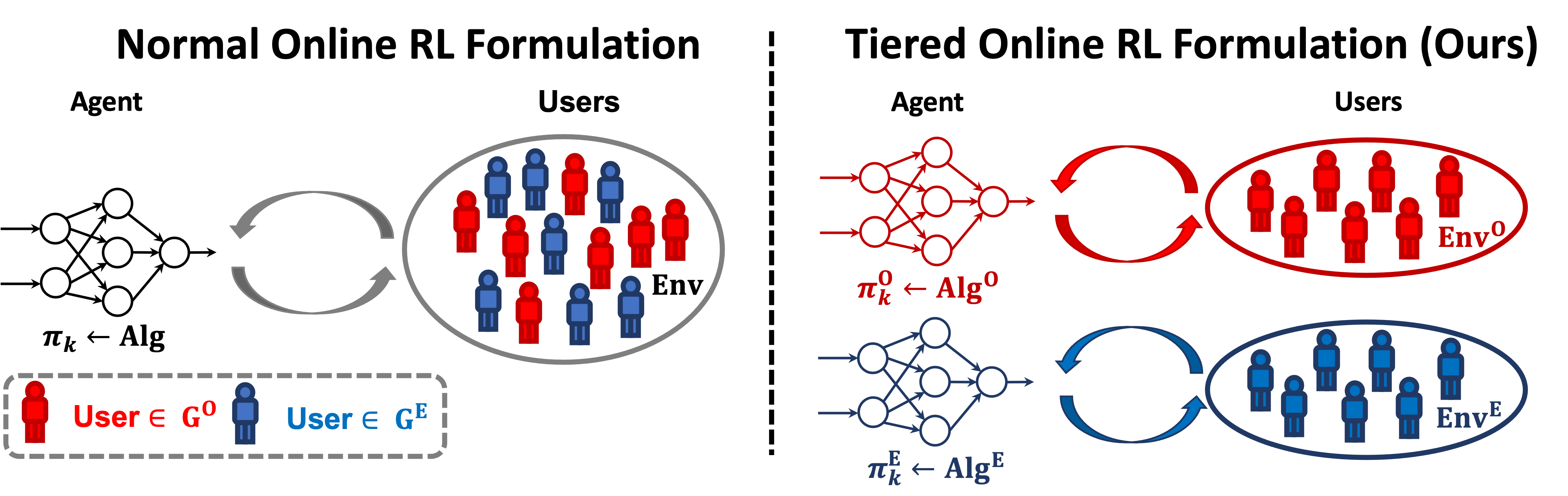
Figure 1: Comparison between the standard setting and our tiered RL setting (#Tiers = 2), where we use red and blue to color users from different groups. The main difference is that, in the standard setting (LHS), the learner does not distinguish users from different groups and treats them equivalently with a single policy $\pi_{k}$ produced by algorithm Alg, while in our setting (RHS), we leverage the tier information and interact with different groups with different policies ${\pi}^{\text{E}}$ and ${\pi}^{\text{O}}$.

To make our objective more clear, we abstract the problem setting into Frw. Framework 1 and compare it with the standard online setting in Fig. 1, where we use $\text{Alg}^{\text{O}}$ and $\text{Alg}^{\text{E}}$ to denote the two algorithms producing policies ${\pi}^{\text{E}}$ and ${\pi}^{\text{O}}$ to interact with users in $\text{G}^{\text{O}}$ and $\text{G}^{\text{E}}$, respectively. To enable theoretical analyses, we do adopt a few simplification assumptions while still modelling the core challenges in the aforementioned scenarios: firstly, at each iteration of Frw. Framework 1, the algorithms will interact with and collect one trajectory from each group, which assumes that users from two groups will come to seek for service in pair with the same frequency. In practice, usually, the users come in random order and the frequencies from different groups are not the same; see Appx. B for why our abstraction is still a valid surrogate and how our results can be generalized. Secondly, for convenience, we only use the samples generated from $\text{G}^{\text{O}}$, because $\text{Alg}^{\text{E}}$ is expected to best exploit the available information and not encouraged to perform intelligent exploration. Nonetheless, our results hold with minor modifications if one also chooses to use trajectories from $\text{G}^{\text{E}}$. Thirdly, we assume that the dynamics and rewards during the interactions with users in different groups are all the same (i.e. $\text{Env}=\text{Env}^{\text{O}}=\text{Env}^{\text{E}}$). It is possible that the users in different tiers can behave differently, and we leave the relaxation of such an assumption to future work.

1 Input: $\text{Env}^{\text{O}}$ and $\text{Env}^{\text{E}}$ // Note that $\text{Env}^{\text{O}}=\text{Env}^{\text{E}}$

2 Initialize $D_{1}\leftarrow\{\}.$

3 for $k=1,2,...,K$ do

4       ${\pi}^{\text{O}}_{k}\leftarrow\text{Alg}^{\text{O}}(D_{k})$; ${\pi}^{\text{E}}_{k}\leftarrow\text{Alg}^{\text{E}}(D_{k})$.

5       ${\pi}^{\text{O}}_{k}$ interacts with customers/users/patients in $\text{G}^{\text{O}}$ (i.e. $\text{Env}^{\text{O}}$), and collect data ${\tau}^{\text{O}}_{k}$.

6       ${\pi}^{\text{E}}_{k}$ interacts with customers/users/patients in $\text{G}^{\text{E}}$ (i.e. $\text{Env}^{\text{E}}$), and collect data ${\tau}^{\text{E}}_{k}$.

7       $D_{k+1}=D_{k}\cup\{{\tau}^{\text{O}}_{k}\}$. // We do not consider to use ${\tau}^{\text{E}}_{k}$ in this paper.

8 end for

Framework 1 The Tiered RL Framework

Similar to the online setting, we use the expected pseudo-regret to measure the performance of the algorithm, which is formalized in Def. 2.1. The key problem we would like to investigate is provable benefits of leveraging the tiered structure by Frw. Framework 1 comparing with the standard online setting:

Is it possible for $\text{Regret}(\text{Alg}^{\text{E}})$ to be strictly lower than any online learning algorithms in certain scenarios, while keeping $\text{Regret}(\text{Alg}^{\text{O}})$ near-optimal?

Note that we still expect regret of $\text{Alg}^{\text{O}}$ to enjoy near-optimal regret guarantees, which is a reasonable requirement as the experience of users in $\text{G}^{\text{O}}$ also matters in many of our motivating applications. We regard the above problem formulation as our first contribution, which is mainly conceptual.

As our second contribution, Sec. 3 shows that $\text{Alg}^{\text{E}}$ has the same minimax gap-independent lower bound as online learning algorithms. This result reveals the difficulty to leverage tiered structure in standard tabular MDPs, and motivates us to investigate the benefits under the gap-dependent setting, which is frequently considered in the Multi-Armed Bandit (MAB) (Lattimore and Szepesvári, 2020; Rouyer and Seldin, 2020) and RL literature (Xu et al., 2021; Simchowitz and Jamieson, 2019).

As our third contribution and our main technical results, Sec. 4 establishes provable benefits of Frw. Framework 1 by proposing a new algorithmic framework and showing $\text{Regret}(\text{Alg}^{\text{E}})$ is constant and independent of the number of episodes $K$, which is in sharp contrast with the $\Omega(\log K)$ regret lower bound for any algorithms in the standard online setting that do not leverage the tiered structure. Specifically, we use Pessimistic Value Iteration (PVI) as $\text{Alg}^{\text{E}}$ for exploitation to interact with $\text{G}^{\text{E}}$, while $\text{Alg}^{\text{O}}$ can be arbitrary online algorithms with near-optimal regret. Concretely, we first study stochastic MABs as a warm-up, where we choose $\text{Alg}^{\text{E}}$ to be LCB (Lower Confidence Bonus), a degenerated version of PVI in bandits, and choose UCB (Upper Confidence Bonus) as $\text{Alg}^{\text{O}}$ for a concrete case study. We prove that $\text{Alg}^{\text{E}}$ can achieve constant pseudo-regret $\widetilde{O}(\sum_{\Delta_{i}>0}(A-i)\Big{(}\frac{1}{\Delta_{i}}-\frac{\Delta_{i}}{\Delta_{i-1}^{2}}\Big{)})$ with $A$ being the number of actions and $\Delta_{i}$’s being the gaps with $\Delta_{1}\geq...\geq\Delta_{A-1}\geq\Delta_{A}=0$, while $\text{Alg}^{\text{O}}$ is near-optimal due to the regret guarantee of UCB. After that, Sec. 4.2 extends the success of PVI to tabular MDPs, and establishes results that apply to a wide range of online algorithms $\text{Alg}^{\text{O}}$ with near-optimal regret. Although the benefits of pessimism have been widely recognized in offline RL (Jin et al., 2021), to our knowledge, we are the first to study PVI in a gap-dependent online setting. We also contribute several novel techniques for overcoming the difficulties in achieving constant regret, and defer their summary to Sec. 4.2. Moreover, in Appx.H, we report experiment results to demostrate the advantage of leveraging tiered structure as predicted by theory.

Closest Related Work Due to space limit, we only discuss the closest related work here and defer the rest to Appx. A. To our knowledge, there is no previous works on leveraging tiered structure in MDPs. In the bandit setting, there is a line of related works studying decoupling exploration and exploitation (Avner et al., 2012; Rouyer and Seldin, 2020), where (Rouyer and Seldin, 2020) studied “best of both worlds” methods and reported a similar constant regret. First, in stochastic bandits, there are many cases when our result is tighter than theirs, (see a detailed comparison in Sec. 4.1), and more importantly, our methods can naturally extend to RL (i.e., MDPs), whereas a similar extension of their techniques can run into serious difficulties: they relied on importance sampling to provide unbiased off-policy estimation for policy value, which incurs the infamous “curse of horizon”, a.k.a., a sample complexity exponential in the planning horizon $H$ in long-horizon RL (see examples in Sec. 2 in (Liu et al., 2018)). Our approach overcomes this difficulty by developing a pessimism-based learning framework, which is fundamentally different from their approach and requires several novel techniques in the analyses. Second, they did not provide any guarantee for the regret of exploration algorithm, whereas in our results the regret of $\text{Alg}^{\text{O}}$ can be near-optimal, which we believe is also important as the experience of users in $\text{G}^{\text{O}}$ also matters in many of our motivating applications. Third, their bandit results require a unique best arm, whereas we allow the optimal arms/policies to be non-unique, which can cause non-trivial difficulties in the analyses as we will discuss in Sec. 4.2.3.

2 Preliminary and Problem formulation

Stochastic Multi-Armed Bandits (MABs)  The MAB model consists of a set of arms $\mathcal{A}=\{1,2,...,A\}$. When sampling an arm $i\in\mathcal{A}$, the agent observes a random variable $r_{i}\in[0,1]$. We use $\mu_{i}=\mathbb{E}[r_{i}]$ to denote the mean value for arm $i$ for each $i\in\mathcal{A}$. We allow the optimal arms to be non-unique. For simplicity of notation, we assume the arms are ordered such that $\mu_{1}\leq\mu_{2}...\leq\mu_{A}$.

Finite-Horizon Tabular Markov Decision Processes (MDPs)  For the reinforcement learning (RL) setting, we consider the episodic tabular MDPs denoted by $M(\mathcal{S},\mathcal{A},H,P,r)$, where $\mathcal{S}$ is the finite state space, $\mathcal{A}$ is the finite action space, $H$ is the horizon length, and ${\mathbb{P}}=\{{\mathbb{P}}_{h}\}_{h=1}^{H}$ and $r=\{r_{h}\}_{h=1}^{H}$ are the time-dependent transition and reward functions, respectively. We assume all steps share the state and action space (i.e. $\mathcal{S}_{1}=\mathcal{S}_{2}...=\mathcal{S}_{H}=\mathcal{S}$, $\mathcal{A}_{1}=\mathcal{A}_{2}...=\mathcal{A}_{H}=\mathcal{A}$) while the transition and reward functions can be different. At the beginning of each episode, the environment will start from a fixed initial state $s_{1}$ (w.l.o.g.). Then, for each time step $h\in[H]$, the agent selects an action $a_{h}\in\mathcal{A}$ based on the current state $s_{h}$, receives the reward $r_{h}(s_{h},a_{h})$, and observes the system transition to the next state $s_{h+1}$, until $s_{H+1}$ is reached. W.l.o.g., we assume the reward function $r$ is deterministic and our results can be easily extended to handle stochastic rewards.

A time-dependent policy is specified as $\pi=\{\pi_{1},\pi_{2},...,\pi_{H}\}$ with $\pi_{h}:\mathcal{S}\to\Delta(\mathcal{A})$ for all $h\in[H]$. Here $\Delta(\mathcal{A})$ denotes the probability simplex over the action space. With a slight abuse of notation, when $\pi_{h}$ is a deterministic policy, we use $\pi_{h}:\mathcal{S}\to\mathcal{A}$ to refer to a deterministic mapping. $V^{\pi}_{h}(s)$ and $Q^{\pi}_{h}(s,a)$ denote the value function and Q-function at step $h\in[H]$, which are defined as: $V^{\pi}_{h}(s)=\mathbb{E}[\sum_{h^{\prime}=h}^{H}r_{h^{\prime}}(s_{h^{\prime}},a_{h^{\prime}})|s_{h}=s,\pi],\quad Q^{\pi}_{h}(s,a)=\mathbb{E}[\sum_{h^{\prime}=h}^{H}r_{h^{\prime}}(s_{h^{\prime}},a_{h^{\prime}})|s_{h}=s,a_{h}=a,\pi].$

We use $V^{*}_{h}(\cdot):=\max_{\pi}V^{\pi}_{h}(\cdot)$ and $Q^{*}_{h}(\cdot,\cdot)=\max_{\pi}Q^{\pi}_{h}(\cdot,\cdot)$ to refer to the optimal state/action-value functions, and $\Pi^{*}(s_{h}):=\{a_{h}|Q^{*}(s_{h},a_{h})=V^{*}_{h}(s_{h})\}$ to denote the collection of all optimal actions at state $s_{h}$. With an abuse of notation, we define $\Pi^{*}:=\{\pi:V_{1}^{\pi}(s_{1})=V_{1}^{*}(s_{1})\}$, i.e., the set of policies that maximize the total expected return. In this paper, when we say that the MDP has “unique optimal (deterministic) policy”, it is up to the occupancy measure, that is, all policies in $\Pi^{*}$ share the same state-action occupancy $d^{\pi}(s_{h},a_{h}):=\Pr(S_{h}=s_{h},A_{h}=a_{h}|S_{1}=s_{1},\pi)$ for all $h\in[H],s_{h}\in\mathcal{S}_{h},a_{h}\in\mathcal{A}_{h}$. In the following, we use $|\Pi^{*}|=1$ to refer to the case of unique optimal (deterministic) policy, where the cardinality of $\Pi^{*}$ is counted up to the equivalence of occupancies. Besides, for any function $V:\mathcal{S}\rightarrow{\mathbb{R}}$, we denote ${\mathbb{P}}_{h}V(s_{h},a_{h}):=\mathbb{E}_{s_{h+1}\sim{\mathbb{P}}_{h}(\cdot|s_{h},a_{h})}[V(s_{h+1})]$.

Gap-Dependent Setting  We follow the standard formulation of gap-dependent setting in previous bandits (Lattimore and Szepesvári, 2020) and RL literature (Simchowitz and Jamieson, 2019; Xu et al., 2021; Dann et al., 2021). In bandits, the gap w.r.t. arm $i$ is defined as $\Delta_{i}:=\max_{j\in[A]}\mu_{j}-\mu_{i},\forall i\in[A]$, and we assume that there exists a strictly positive value $\Delta_{\min}$ such that, either $\Delta_{i}=0$ or $\Delta_{i}\geq\Delta_{\min}$. For tabular RL setting, we define $\Delta_{h}(s_{h},a_{h}):=V^{*}(s_{h})-Q^{*}(s_{h},a_{h}),\forall h\in[H],s_{h}\in\mathcal{S}_{h},a_{h}\in\mathcal{A}_{h}$. We use the same notation $\Delta_{\min}$ to refer to the minimal gap in tabular setting and assume that either $\Delta_{h}(s_{h},a_{h})=0$ or $\Delta_{h}(s_{h},a_{h})\geq\Delta_{\min}$.

Performance Measure  We use Pseudo-Regret defined below to measure the performance of $\text{Alg}^{\text{O}}$ and $\text{Alg}^{\text{E}}$. In the following, we will also use “exploitation regret” to refer to $\text{Regret}_{K}(\text{Alg}^{\text{E}})$.

Definition 2.1 (Pseudo-Regret).

We define the regret of $\text{Alg}^{\text{O}}$ and $\text{Alg}^{\text{E}}$ to be:

$$\text{Regret}_{K}(\text{Alg}^{\text{O}}):= \mathbb{E}\left[\sum_{k=1}^{K}V_{1}^{*}(s_{1})-V_{1}^{{\pi}^{\text{O}}_{k}}(s_{1})\right];\quad\text{Regret}_{K}(\text{Alg}^{\text{E}}):=\mathbb{E}\left[\sum_{k=1}^{K}V_{1}^{*}(s_{1})-V_{1}^{{\pi}^{\text{E}}_{k}}(s_{1})\right],$$

where ${\pi}^{\text{O}}_{k}$ and ${\pi}^{\text{E}}_{k}$ are generated according to the procedure in Framework Framework 1 and the expectation is taken over the randomness in data generation and algorithms.

3 Lower Bound of $\text{Regret}(\text{Alg}^{\text{E}})$ without Gap Assumption

In this section, we show that, in normal tabular RL setting, for arbitrary algorithm pair $(\text{Alg}^{\text{O}},\text{Alg}^{\text{E}})$, even if we do not constrain $\text{Alg}^{\text{O}}$ to be near-optimal, the regret of $\text{Alg}^{\text{E}}$ has the same minimax lower bound as algorithms in online setting. We defer the formal statement and proof to Appendix C.1.

Theorem 3.1.

[Lower Bound for $\text{Alg}^{\text{E}}$ without Gap Assumption] There exist positive constants $c,\varepsilon_{0},\delta_{0}$, such that, for arbitrary $S\geq 4,A\geq 2,H\geq 2,K\geq\frac{c}{\varepsilon_{0}^{2}}H^{3}SA$, and arbitrary algorithm pair $(\text{Alg}^{\text{O}},\text{Alg}^{\text{E}})$, there must exist a hard tabular MDP $M_{hard}$, $\mathbb{E}_{(\text{Alg}^{\text{O}},\text{Alg}^{\text{E}}),M_{hard}}\left[\sum_{k=1}^{K}V^{*}-V^{{\pi}^{\text{E}}_{k}}\right]\geq\delta_{0}\sqrt{cH^{3}SAK},$ where the expectation is taken over the randomness of algorithms and MDP.

The theorem above is stating that, comparing with the regret lower bound for online algorithms $\widetilde{O}(\sqrt{H^{3}SAK})$ in Theorem 9 of Domingues et al. (2021), the exploitation algorithm cannot reduce the dependence on any of parameters $H,S,A,K$ in hard MDPs, even if we allow $\text{Alg}^{\text{O}}$ to sacrifice its performance to gather the best possible data for $\text{Alg}^{\text{E}}$. Also, the lower bound would still hold even if we allow both $\text{Alg}^{\text{O}}$ and $\text{Alg}^{\text{E}}$ to additionally use the data ${\tau}^{\text{E}}$ generated by ${\pi}^{\text{E}}$. This negative result implies that without any further assumptions, the separation is not beneficial from a minimax optimality perspective, and we can simply choose both $\text{Alg}^{\text{E}}$ and $\text{Alg}^{\text{O}}$ to be the same near-optimal online algorithm as without worrying about separating them.

However, in the next section, we will show that, in tabular MDPs with strictly positive gaps, in contrast with the $\Omega(\log K)$ lower bound for online algorithms, we can have $\text{Alg}^{\text{E}}$ such that its regret is constant and independent on the number of time horizon $K$, which reveals the fundamental differences between the pure online setting and the Tiered RL setting considered in this paper.

4 Pessimism in the Face of Uncertainty and Constant Regret

In this section, we consider the gap-dependent setting and contribute to identifying the possibility to achieve constant regret by using pessimistic algorithms for $\text{Alg}^{\text{E}}$. Intuitively, the main reason why PVI can lead to a constant regret is that the quality of the policy returned by PVI is positively correlated to the accumulation of optimal trajectories in the dataset $D$, which is directly connected with $\text{Regret}(\text{Alg}^{\text{O}})$. As a result, on the one hand, the regret minimization objective of $\text{Alg}^{\text{E}}$ coincidentally aligns with the optimality constraint of $\text{Alg}^{\text{O}}$. On the other hand, thanks to the positive gap assumption, ${\pi}^{\text{E}}$ will gradually converge to the optimal policy with high probability when $\text{Alg}^{\text{E}}$ is PVI, so there will be no regret after that. In Sec. 4.1, we start with stochastic MAB as a warm-up, and in Sec. 4.2 we extend our success to tabular RL setting. We defer the proofs in this section to Appendix D.

4.1 Warm-Up: Gap-Dependent Regret Bound for Stochastic Multi-Armed Bandits

1Initilize: $\alpha>1;\quad N_{i}(1)\leftarrow 0,~{}\widehat{\mu}_{i}(1)\leftarrow 0,~{}\forall i\in\mathcal{A};\quad f(k):=1+16A^{2}(k+1)^{2}$

2 for $k=1,2,...,K$ do

3       ${\pi}^{\text{O}}_{k}\leftarrow\arg\max_{i}\widehat{\mu}_{i}(k)+\sqrt{\frac{2\alpha\log f(k)}{N_{i}(k)}},\quad\quad{\pi}^{\text{E}}_{k}\leftarrow\arg\max_{i}\widehat{\mu}_{i}(k)-\sqrt{\frac{2\alpha\log f(k)}{N_{i}(k)}}.$

4       Interact with $\text{G}^{\text{E}}$ and $\text{G}^{\text{O}}$ by ${\pi}^{\text{E}}_{k}$ and ${\pi}^{\text{O}}_{k}$, and observe reward $r({\pi}^{\text{E}}_{k})$ and $r({\pi}^{\text{O}}_{k})$, respectively.

5       for $i=1,2,...,A$ do

6             $N_{i}(k+1)\leftarrow N_{i}(k)+\mathbb{I}[{\pi}^{\text{O}}_{k}=i];\qquad\widehat{\mu}_{i}(k+1)\leftarrow\widehat{\mu}_{i}(k)\frac{N_{i}(k)}{N_{i}(k+1)}+r({\pi}^{\text{O}}_{k})\frac{\mathbb{I}[{\pi}^{\text{O}}_{k}=i]}{{N_{i}(k+1)}}.$

7       end for

8      

9 end for

Algorithm 2 UCB-Exploration-LCB-Exploitation

Our main algorithm for bandit setting is shown in Alg Framework 1, where we consider the UCB algorithm (Lattimore and Szepesvári, 2020) as $\text{Alg}^{\text{O}}$ and choose the LCB as $\text{Alg}^{\text{E}}$, which flips the sign of the bonus term in UCB. We use $N_{i}(k)$ to denote the number of times that arm $i$ was pulled previous to step $k$, and use $\widehat{\mu}_{i}$ to record the empirical average of arm $i$. Besides, we assume $1/N_{i}(\cdot)=+\infty$ if $N_{i}(\cdot)=0$, which implies that at the first $|\mathcal{A}|$ steps the algorithm will pull each arm one by one. Moreover, as we will show later, the choice of $\alpha>1$ is crucial to avoiding dependence on $K$ in $\text{Regret}(\text{Alg}^{\text{E}})$ with our techniques. For Alg. 2, we have the following guarantee:

Theorem 4.1.

[Exploitation Regret] In Algorithm 2, by choosing arbitrary $\alpha>1$, there exists an absolute constant $c$, such that, for arbitrary $K\geq 1$, the pseduo-regret of $\text{Alg}^{\text{E}}$ is upper bounded by: $\text{Regret}_{K}(\text{Alg}^{\text{E}})\leq\widetilde{O}\left(\frac{A}{\alpha-1}+\alpha\sum_{\Delta_{i}>0}(A-i)\Big{(}\frac{1}{\Delta_{i}}-\frac{\Delta_{i}}{\Delta_{i-1}^{2}}\Big{)}\right)$ where $\Delta_{0}:=\infty$ so $\frac{\Delta_{1}}{\Delta_{0}^{2}}=0$.

Our result implies that by choosing PVI as $\text{Alg}^{\text{E}}$, we can achieve constant regret while keeping $\text{Alg}^{\text{O}}$ near-optimal. Besides the advantages discussed in the related work paragraph in Sec. 1, our guarantee is also more favorable in certain cases compared to the $O(\sqrt{\frac{A}{\Delta_{\min}}}\sqrt{\sum_{\Delta_{i}>0}\frac{1}{\Delta_{i}}})$ result in Rouyer and Seldin (2020): while it is not easy to verify whether our guarantee dominates theirs, in many cases ours can be strictly better (or at least no worse) than theirs. For example, consider the following two representative cases: $\Delta_{1}=\Delta_{2}=...\Delta_{A-1}=\Delta_{\min}$ (uniform gap) and $\Delta_{1}=\Delta_{2}=...=\Delta_{A-2}\gg\Delta_{A-1}=\Delta_{\min}$ (small last gap); our result achieves $\widetilde{O}(\frac{A}{\Delta_{\min}})$ and $\widetilde{O}(\frac{1}{\Delta_{\min}})$, respectively, in contrast to their $\widetilde{O}(\frac{A}{\Delta_{\min}})$ and $\widetilde{O}(\frac{\sqrt{A}}{\Delta_{\min}})$.

Proof Sketch: The proof consists of two novel technique lemmas with a carefully chosen failure rate $\delta_{k}\sim O(1/k^{\Theta(\alpha)})$ so that the accumulative failure probability $\sum_{k=1}^{\infty}\delta_{k}<+\infty$. The first one is Lem. 4.2, where we show that w.p. $1-\delta_{k}$, LCB will not prefer $i$ with $\Delta_{i}>0$ as long as another better arm has been visited enough times in the dataset. The second step is to identify a key property of UCB algorithm as stated in Lem. 4.3, where we provide a high probability upper bound that $N_{i}(k)\leq k/\lambda$ if $k\geq\widetilde{\Theta}({\lambda}/{\Delta_{i}^{2}})$ for arbitrary $\lambda\in[1,4A]$, and it serves to indicate that the condition required by the success of LCB is achievable as long as $k$ is large enough .

Lemma 4.2.

[Blessing of Pessimism] With the choice that $f(k)=1+16A^{2}(k+1)^{2}$, for arbitrary $i$ with $\Delta_{i}>0$, for the LCB algorithm in Alg 2, and arbitrary $j$ satisfying $\Delta_{j}<\Delta_{i}$, we have: $\Pr\left(\{i={\pi}^{\text{E}}_{k}\}\cap\{\Delta_{j}<\Delta_{i}\}\cap\left\{N_{j}(k)\geq\frac{8\alpha\log f(k)}{(\Delta_{j}-\Delta_{i})^{2}}\right\}\right)\leq\frac{2}{k^{2\alpha}}.$

Lemma 4.3.

[Property of UCB] With the choice that $f(k)=1+16A^{2}(k+1)^{2}$, there exists a constant $c$, for arbitrary $i$ with $\Delta_{i}>0$ and arbitrary $\lambda\in[1,4A]$, in UCB algorithm, we have: $\Pr(N_{i}(k)\geq\frac{k}{\lambda})\leq\frac{2}{k^{2\alpha-1}},\quad\forall k\geq\lambda+c\cdot\frac{\alpha\lambda}{\Delta_{i}^{2}}\log(1+\frac{\alpha A}{\Delta_{\min}}).$

Directly combining the above two results, we can obtain an upper bound for $\text{Regret}(\text{Alg}^{\text{E}})$ of order $\widetilde{O}(A/\Delta_{\min}^{-2})$, which is already independent of $K$. To achieve better dependence on $\Delta_{\min}$ in the regret, we conduct a finer analysis. For each arm $i$ with $\Delta_{i}>0$, we separate all the arms including $i$ into two groups based on whether its gap exceeds $\Delta_{i}/2$: $G^{\text{lower}}_{i}=\{j:\Delta_{j}>\Delta_{i}/2\}$ and $G^{\text{upper}}_{i}=\{j:\Delta_{j}\leq\Delta_{i}/2\}$. As a result of Lem. 4.2, we know that ${\pi}^{\text{E}}_{k}$ will not prefer arm $i$ as long as there exists $j\in G^{\text{upper}}_{i}$ such that $N_{j}(k)=\widetilde{\Omega}(4\Delta^{-2}_{i})=\widetilde{\Omega}(\Delta_{i}^{-2})$. Based on Lem. 4.3, we know it is true with high probability, as long as $k\geq\widetilde{\Theta}(A\cdot\Delta_{i}^{-2})$, since at that time $N_{l}(k)\leq k/A$ holds for arbitrary $l\in G^{\text{lower}}_{i}$, which directly implies that $\max_{j:j\in G^{\text{upper}}_{i}}N_{j}(k)\geq\widetilde{\Omega}(\Delta_{i}^{-2})$. Then, combining Lem. 4.2, with high probability, the regret resulting from taken arm $i$ cannot be higher than $\widetilde{\Theta}(A\cdot\Delta_{i}^{-2})\cdot\Delta_{i}=\widetilde{\Theta}(A\cdot\Delta_{i}^{-1})$, which results in a $\widetilde{O}(\sum_{\Delta_{i}>0}A/\Delta_{i})$ regret bound. As for the techniques leading to the further improvement in our final result, please refer to Lem. D.1 and the proof of Thm. 4.1 in Appx. D.

4.2 Constant Regret of $\text{Alg}^{\text{E}}$ in Tabular MDPs

In this section, we establish constant regret of $\text{Alg}^{\text{E}}$ based on realistic conditions for $\text{Alg}^{\text{O}}$ and $\text{Alg}^{\text{E}}$. We highlight the key steps of our analysis and our technical contributions here.

First of all, in Sec.4.2.1, we propose the concrete PVI algorithm, and inspired by the clipping trick used for optimistic online algorithms (Simchowitz and Jamieson, 2019), we develop a high-probability gap-dependent upper bound for the sub-optimality of ${\pi}^{\text{E}}$, which is related to the accumulation of the optimal trajectories in dataset $D_{k}$. Secondly, in Sec. 4.2.2, we first introduce a general condition (Cond. 4.6) for the chocie of $\text{Alg}^{\text{O}}$, based on which we quantify the accumulation of optimal trajectories in $D_{k}$ with the regret of $\text{Alg}^{\text{O}}$, and connect the exploration by $\text{Alg}^{\text{O}}$ and the optimality of $\text{Alg}^{\text{E}}$. We also supplement some details about how to relax such a condition and inherit the guarantees by the doubling-trick in Appx. G, which may be of independent interest. In Sec. 4.2.3, i.e. the last part of analysis, we bring the above two steps together and complete the proof. However, there is an additional challenge when the tabular MDP has multiple deterministic optimal policies, which is possible when there are non-unique optimal actions at some states. We overcome this difficulty by Thm. 4.8 about policy coverage. To our knowledge, the only paper that runs into a similar challenge is (Papini et al., 2021), and they bypass the difficulty by assuming the uniqueness of optimal policy. Finally, Section 4.2.4 provide some interpretation and implications of our results.

4.2.1 Pessimistic Value Iteration as $\text{Alg}^{\text{E}}$ and its Property

1Input: Episode number $K$; Confidence level $\{\delta_{k}\}_{k=1}^{K}$; Bonus function $\textbf{Bonus}(\cdot,\cdot)$

2 for $k=1,2,...,K$ do

3       $\{b_{k,1}(\cdot,\cdot),b_{k,2}(\cdot,\cdot),...,b_{k,H}(\cdot,\cdot)\}\leftarrow\textbf{Bonus}(D_{k},\delta_{k}).$ // Compute bonus function for PVI.

4       for $h=H,H-1,...,1$ do

5             for $s_{h}\in\mathcal{S}_{h},a_{h}\in\mathcal{A}_{h}$ do

6                   $N_{k,h}(s_{h},a_{h})\leftarrow$ the number of times $s_{h},a_{h}$ occurs in the dataset $D_{k}$.

7                   $N_{k,h}(s_{h},a_{h},s_{h+1})\leftarrow$ the number of times $(s_{h},a_{h},s_{h+1})$ occurs in the dataset $D_{k}$.

8                   ${\widehat{\mathbb{P}}}_{k,h}(\cdot|s_{h},a_{h})\leftarrow\begin{cases}0,\quad&\text{if }N_{k,h}(s_{h},a_{h})=0;\\ \frac{N_{k,h}(s_{h},a_{h},\cdot)}{N_{k,h}(s_{h},a_{h})},\quad&\text{otherwise}.\end{cases}$

9                  

10             end for

11            ${\widehat{Q}}_{k,h}(\cdot,\cdot)\leftarrow\max\{R(\cdot,\cdot)+{\widehat{\mathbb{P}}}_{k,h}{\widehat{V}}_{k,h+1}(\cdot,\cdot)-b_{k,h}(\cdot,\cdot),0\}.$

12             ${\widehat{V}}_{k,h}(\cdot)=\max_{a_{h}\in\mathcal{A}}{\widehat{Q}}_{k,h}(\cdot,a_{h}),\quad{\pi}^{\text{PVI}}_{k,h}(\cdot)\leftarrow\operatorname*{arg\,max}_{a}{\widehat{Q}}_{k,h}(\cdot,a).$

13       end for

14      ${\pi}^{\text{E}}_{k}\leftarrow\{{\pi}^{\text{PVI}}_{k,1},{\pi}^{\text{PVI}}_{k,2},...{\pi}^{\text{PVI}}_{k,H}\}$

15       // Step 2: Use $\text{Alg}^{\text{O}}$ satisfying Cond. 4.6 to compute ${\pi}^{\text{O}}_{k}$ for $\text{G}^{\text{O}}$

16       ${\pi}^{\text{O}}_{k}\leftarrow\text{Alg}^{\text{O}}(D_{k}).$

17       // Step 3: Sample trajectories and collect new data

18       Interact with $\text{G}^{\text{E}}$ and $\text{G}^{\text{O}}$ by ${\pi}^{\text{E}}_{k}$ and ${\pi}^{\text{O}}_{k}$, and observe ${\tau}^{\text{E}}_{k}$ and ${\tau}^{\text{O}}_{k}$, respectively.

19       $D_{k+1}\leftarrow D_{k}\cup\{{\tau}^{\text{O}}_{k}\}$.

20 end for

Algorithm 3 Tiered-RL Algorithm with Pessimistic Value Iteration as $\text{Alg}^{\text{E}}$

The full details of our algorithm for tiered RL setting is provided in Alg. 3, where we use PVI as $\text{Alg}^{\text{E}}$. Here we do not specify a concrete Bonus function, but provide general results for a range of qualified bonus functions satisfying Cond. 4.4 below. Cond. 4.4 can be satisfied by many bonus term considered in online literatures, and we briefly dicuss some examples in Appx. F.1.

Condition 4.4 (Condition on Bonus Term for $\text{Alg}^{\text{E}}$).

We define the following event at iteration $k\in[K]$ during the running of Alg. 3: $\mathcal{E}_{\textbf{Bonus},k}:=\bigcap_{\begin{subarray}{c}h\in[H],s_{h}\in\mathcal{S}_{h},a_{h}\in\mathcal{A}_{h}\end{subarray}}\Big{\{}\{|\widehat{\mathbb{P}}_{k,h}{\widehat{V}}_{k,h+1}(s_{h},a_{h})-{\mathbb{P}}_{h}{\widehat{V}}_{k,h+1}(s_{h},a_{h})|<b_{k,h}(s_{h},a_{h})\}\cap\{b_{k,h}(s_{h},a_{h})\leq B_{1}\sqrt{\frac{\log(B_{2}/\delta_{k})}{N_{k,h}(s_{h},a_{h})}}\}\Big{\}}$ where $B_{1}$ and $B_{2}$ are parameters depending on $S,A,H$ and $\Delta$ but independent of $\delta_{k}$, $k$. We assume that, Bonus function satisfies that, in Alg. 3, given arbitrary sequence $\{\delta_{k}\}_{k=1}^{K}$ with $\delta_{1},\delta_{2},...,\delta_{K}\in(0,1/2)$, at arbitrary iteration $k\in[K]$, we have $\Pr(\mathcal{E}_{\textbf{Bonus},k})\geq 1-\delta_{k}$.

Next, we provide an upper bound for the sub-optimality gap of ${\pi}^{\text{PVI}}_{k}$ with the clipping operator $\text{Clip}[x|\varepsilon]:=x\cdot\mathbb{I}[x\geq\varepsilon]$. Previous upper bounds of PVI (e.g., Theorem 4.4 of Jin et al., 2021) do not leverage the strictly positive gap and can be much looser when $N_{k,h}$ is large, and directly applying those results to our analysis would result in a regret scaling with $\sqrt{K}$.

Theorem 4.5.

By running Algorithm 3 with confidence level $\delta_{k}$, a function Bonus satisfying Condition 4.4, and a dataset $D=\{\tau_{1},...\tau_{k}\}$ consisting of $k$ complete trajectories generated by executing a sequence of policies $\pi_{1},...,\pi_{k}$, on the event $\mathcal{E}_{\textbf{Bonus}}$ defined in Condition 4.4:

$$V^{*}_{1}(s_{1})-V_{1}^{{\pi}^{\text{PVI}}_{k}}(s_{1})\leq 2\mathbb{E}_{\pi^{*}}\left[\sum_{h=1}^{H}\text{Clip}\left[\left.\min\left\{H,2B_{1}\sqrt{\frac{\log(B_{2}/\delta_{k})}{N_{k,h}(s_{h},a_{h})}}\right\}\right|\varepsilon_{\text{Clip}}\right]\right].$$ (1)

where $\pi^{*}$ can be an arbitrary optimal policy, $\varepsilon_{\text{Clip}}:=\frac{\Delta_{\min}}{2H+2}$ if $|\Pi^{*}|=1$ and $\varepsilon_{\text{Clip}}:=\frac{d_{\min}\Delta_{\min}}{2SAH}$ if $|\Pi^{*}|>1$, where $d_{\min}:=\min_{\pi\in\Pi^{*},h\in[H],s_{h}\in\mathcal{S}_{h},a_{h}\in\mathcal{A}_{h}}d^{\pi}(s_{h},a_{h})$ subject to $d^{\pi}(s_{h},a_{h})>0$.

4.2.2 Choice and Analysis of $\text{Alg}^{\text{O}}$

Next, we introduce our general condition for $\text{Alg}^{\text{O}}$ that the $\text{Alg}^{\text{O}}$ can achieve $O(\log k)$-regret with high probability. It is worth noting that many existing near-optimal online RL algorithms for gap-dependent settings may not directly satisfy the condition (Simchowitz and Jamieson, 2019; Xu et al., 2021; Dann et al., 2021) since they use a fixed confidence interval $\delta$. In Appx. G, we will introduce a more realistic abstraction of those algorithms in Cond. G.1, and discuss in more details about how to close this gap with an algorithm framework inspired by the doubling trick.

Condition 4.6 (Condition on $\text{Alg}^{\text{O}}$).

$\text{Alg}^{\text{O}}$ is an algorithm which returns deterministic policies at each iteration, and for arbitrary ${k}\geq 2$, we have: $\Pr\big{(}\sum_{{\widetilde{k}}=1}^{k}V^{*}_{1}(s_{1})-V^{{\pi}^{\text{O}}_{\widetilde{k}}}_{1}(s_{1})>C_{1}+\alpha C_{2}\log{k}\big{)}\leq\frac{1}{{k}^{\alpha}},$ where $C_{1},C_{2}$ are parameters only depending on $S,A,H$ and gap $\Delta$ and independent of ${k}$.

Implication of Condition 4.6 for $\text{Alg}^{\text{O}}$ Intuitively, low regret implies high accumulation of optimal trajectories in the dataset collected by $\text{Alg}^{\text{O}}$. We formalize this intuition in Thm. 4.7 by establishing the relationship between the regret of $\text{Alg}^{\text{O}}$, $d^{\pi^{*}}$ and $\sum_{{\widetilde{k}}=1}^{k}d^{{\pi}^{\text{O}}_{\widetilde{k}}}(s_{h},a_{h})$ (the expectation of $N_{k,h}$).

Theorem 4.7.

For an arbitrary sequence of deterministic policies $\pi_{1},\pi_{2},...,\pi_{k}$, there must exist a sequence of deterministic optimal policies $\pi_{1}^{*},\pi_{2}^{*},...,\pi_{k}^{*}$, such that $\forall h\in[H],s_{h}\in\mathcal{S}_{h},a_{h}\in\mathcal{A}_{h}$:

$$\sum_{{\widetilde{k}}=1}^{k}d^{\pi_{\widetilde{k}}}(s_{h},a_{h})\geq\sum_{{\widetilde{k}}=1}^{k}d^{\pi^{*}_{\widetilde{k}}}(s_{h},a_{h})-\frac{1}{\Delta_{\min}}\Big{(}\sum_{{\widetilde{k}}=1}^{k}V^{*}_{1}(s_{1})-V^{\pi_{\widetilde{k}}}_{1}(s_{1})\Big{)}.$$

4.2.3 Main Results and Analysis

The main analysis is based on our discussion about the properties of $\text{Alg}^{\text{E}}$ and $\text{Alg}^{\text{O}}$ in previous sub-sections. In the following, we first discuss the proof sketch for the case when $|\Pi^{*}|=1$. The main idea is to show that the unique $\pi^{*}$ will be “well-covered” by dataset, where we say a policy $\pi^{*}$ is “well-covered” if for each $(s_{h},a_{h})\in\mathcal{S}_{h}\times\mathcal{A}_{h}$ with $d^{\pi^{*}}(s_{h},a_{h})>0$, $N_{k,h}(s_{h},a_{h})$ can strictly increase so that the RHS of Eq.(1) in Thm. 4.5 will gradually decay to zero (e.g. $N_{k,h}(s_{h},a_{h})\geq\widetilde{O}(k)$). To show this, the key observation is that, with high probability, $N_{k,h}(s_{h},a_{h})$ will not deviate too much from its expectation $\sum_{\widetilde{k}}d^{\pi_{\widetilde{k}}}(s_{h},a_{h})$ (Lem. F.8), and can be lower bounded by $\sum_{{\widetilde{k}}=1}^{k}d^{\pi_{\widetilde{k}}^{*}}(s_{h},a_{h})-O(\log k)=kd^{\pi^{*}}(s_{h},a_{h})-O(\log k)$ as a result of Thm. 4.7. As a result, the clipping operator in Eq.(1) will take effects as long as $k$ is large enough, and ${\pi}^{\text{PVI}}_{k}$ will converge to the optimal policy with no regret. All that remains is to show the regret under failure events is also at the constant level because we choose a gradually decreasing failure rate $O(\frac{1}{k^{\alpha}})$, and $\lim_{K\rightarrow\infty}\sum_{k=1}^{K}O(\frac{1}{k^{\alpha}})<\infty$ as long as $\alpha>1$.

However, when $|\Pi^{*}|>1$, the analysis becomes more challenging. The main difficulty is that, when the optimal policy is not unique, it is not obvious about the existence of “well-covered” $\pi^{*}$, since it is not guarantee that how much similarity is shared by the sequence of policies $\pi_{1}^{*},...\pi^{*}_{k}$, especially when $|\Pi^{*}|$ is exponentially large (e.g. $|\Pi^{*}|=\Omega((SA)^{H})$). We overcome this difficulty by proving the existence of “well-covered” policy in the theorem stated below:

Theorem 4.8.

[The existance of well-covered optimal policy] Given an arbitrary tabular MDP, and an arbitrary sequence of deterministic optimal policies $\pi^{*}_{1},\pi^{*}_{2},...\pi^{*}_{k}$ ($\pi^{*}_{i}$ may not equal to $\pi^{*}_{j}$ for arbitrary $1\leq i<j\leq{k}$ when there are multiple deterministic optimal policies), there exists a (possibly stochastic) policy $\pi^{*}_{\text{cover}}$ such that $\forall h\in[H],\forall(s_{h},a_{h})\in\mathcal{S}_{h}\times\mathcal{A}_{h}$ with $d^{\pi^{*}_{\text{cover}}}(s_{h},a_{h})>0$:

$$\sum_{{\widetilde{k}}=1}^{k}d^{\pi^{*}_{\widetilde{k}}}(s_{h},a_{h})\geq\frac{{k}}{2}\cdot\widetilde{d}^{\pi^{*}_{\text{cover}}}(s_{h},a_{h}),~{}\text{with}~{}\widetilde{d}^{\pi^{*}_{\text{cover}}}(\cdot,\cdot):=\max\left\{\frac{d^{*}_{h,\min}(\cdot,\cdot)}{(|\mathcal{Z}_{h,\text{div}}|+1)H},d^{\pi^{*}_{\text{cover}}}(\cdot,\cdot)\right\}.$$

where $\mathcal{Z}_{h,\text{div}}^{*}:=\{(s_{h},a_{h})\in\mathcal{S}_{h}\times\mathcal{A}_{h}|\exists\pi^{*},\widetilde{\pi}^{*}\in\Pi^{*},~{}s.t.~{}d^{\pi^{*}}(s_{h})>0,~{}d^{\widetilde{\pi}^{*}}(s_{h})=0\}$, and $d^{*}_{h,\min}(s_{h},a_{h}):=\min_{\pi^{*}\in\Pi^{*}}d^{\pi^{*}}(s_{h},a_{h})$ subject to $d^{\pi^{*}}(s_{h},a_{h})>0$.

Here we provide some explanation to the above result. According to the definition, $\mathcal{Z}^{*}_{h,div}$ is the set including the state-action pairs which can be covered by some deterministic policies but is not reachable by some other deterministic policies, and therefore $|\mathcal{Z}^{*}_{h,div}|\leq SA$ (or even $|\mathcal{Z}^{*}_{h,div}|\ll SA$). Besides, $d^{*}_{h,\min}(s_{h},a_{h})$ denotes the minimal occupancy over all possible deterministic optimal policies which can hit $s_{h},a_{h}$, and therefore, is no less than $d_{\min}$ defined in Thm. 4.5. As a result, we know there exists a “well-covered” $\pi^{*}_{\text{cover}}$, since the accumulative density of its arbitrary reachable states can be lower bounded by $O(k)$. Then, following a similar discussion as the case $|\Pi^{*}|=1$, we can finish the proof. We summarize our main result below.

Theorem 4.9.

By running an Algorithm satisfying Condition 4.6 as $\text{Alg}^{\text{O}}$, running Alg 3 as $\text{Alg}^{\text{E}}$ with a bonus term function Bonus satisfying Condition 4.4 and $\delta_{k}=1/k^{\alpha}$, for some constant $\alpha>1$, for arbitrary $K\geq 1$, the exploitation regret of $\text{Alg}^{\text{E}}$ can be upper bounded by:

(i) When $|\Pi^{*}|=1$ (unique optimal deterministic policy):

$$\text{Regret}_{K}(\text{Alg}^{\text{E}})\leq O\Big{(}\sum_{h=1}^{H}\sum_{\begin{subarray}{c}s_{h},a_{h}:\\ d^{\pi^{*}}(s_{h},a_{h})>0\end{subarray}}\Big{(}\frac{C_{1}+C_{2}}{\Delta_{\min}}\log\frac{SAH(C_{1}+C_{2})}{d^{\pi^{*}}(s_{h},a_{h})\Delta_{\min}}+\frac{B_{1}H}{\Delta_{\min}}\log\frac{B_{2}H}{d^{\pi^{*}}(s_{h},a_{h})\Delta_{\min}}\Big{)}\Big{)}.$$

(ii) When $|\Pi^{*}|>1$ (non-unique optimal deterministic policies):

$$\text{Regret}_{K}(\text{Alg}^{\text{E}})\leq O\Big{(}\sum_{h=1}^{H}\sum_{\begin{subarray}{c}s_{h},a_{h}:\\ d^{\pi^{*}_{\text{cover}}}(s_{h},a_{h})>0\end{subarray}}\Big{(}\frac{C_{1}+C_{2}}{\Delta_{\min}}\log\frac{SAH(C_{1}+C_{2})}{\widetilde{d}^{\pi^{*}_{\text{cover}}}(s_{h},a_{h})\Delta_{\min}}+\frac{B_{1}SAH}{d_{\min}\Delta_{\min}}\log\frac{B_{2}SAH}{d_{\min}\Delta_{\min}}\Big{)}\Big{)}.$$

where $\pi^{*}_{\text{cover}}$ and $\widetilde{d}^{\pi^{*}_{\text{cover}}}(s_{h},a_{h})$ are introduced in Theorem 4.8.

4.2.4 Interpretation of Results in Tabular RL

Recall our objective in Sec. 1 is to establish the benefits of leveraging the tiered structure by showing $\text{Regret}_{K}(\text{Alg}^{\text{E}})$ is constant. This contrasts the lower bound of online algorithms that continuously increases with the episode number $K$, which corresponds to the regret suffered by users in $\text{G}^{\text{E}}$ without leveraging the tiered structure, while $\text{Regret}_{K}(\text{Alg}^{\text{O}})$ keeps (near-)optimal as before. In Appx. H, we also provide some simulation results as a verification of our theoretical discovery.

One limitation of our results is that our bounds have additional dependence on $d^{\pi^{*}}$ (or even ${1}/{d^{\pi^{*}}}$) compared to most of the regret bounds in the online setting, although similar dependence on $\log d^{\pi^{*}}$ also appeared in a few recent works (e.g., $\lambda_{h}^{+}$ in Thms. 8 and 9 of Papini et al., 2021). Besides, according to the lower and upper bound of online RL in gap-dependent settings (Simchowitz and Jamieson, 2019), $C_{1}+C_{2}$ in Cond. 4.6 have dependence on $O(\Delta_{\min}^{-1})$, which implies that in the regret bound in Thm. 4.9, the dependence on $\Delta_{\min}$ would be $O(\Delta^{-2}_{\min})$. For the former, in Appx. C.2, we prove a lower bound, showing that $\log\frac{1}{d^{\pi^{*}}}$ is unavoidable when $\text{Alg}^{\text{O}}$ is allowed to behave adversarially without violating Cond. 4.6; for the latter, we note that in the analysis of MAB setting (Sec.4.1), specifying the detailed behavior of $\text{Alg}^{\text{O}}$ can help tighten the bound. Therefore, we conjecture that our results can be improved by putting more constraints on the behavior of $\text{Alg}^{\text{O}}$, which we leave to future work.

5 Conclusion

In this paper, we identify the tiered structure in many real-world applications and study the potential advantages of leveraging it by interacting with users from different groups with different strategies. Under the gap-dependent setting, we provide theoretical evidence of benefits by deriving constant regret for the exploitation policy while maintaining the optimality of the online learning policy.

As for the future work, we propose several potentially interesting directions. (i) As we mentioned in Section 4.2.4, it is worth investigating the possibility of improving the regret bound of $\text{Alg}^{\text{E}}$ by considering a more concrete choice of $\text{Alg}^{\text{O}}$, or maybe other choices for $\text{Alg}^{\text{E}}$. (ii) It would be interesting to relax our constraint on the optimality of $\text{Alg}^{\text{O}}$ by introducing the notion of budget $C$ as the tolerance on the sub-optimality of $\text{Alg}^{\text{O}}$. As a result, our setting and the decoupling exploration and exploitation setting can be regarded as special cases of a more general framework when $C=0$ and $C=\infty$. (iii) We assume that the users from different groups share the same transition and reward function, and it would also be interesting to extend our results to more general settings, where the group ID serves as context and will affect the dynamics (Abbasi-Yadkori and Neu, 2014; Modi et al., 2018). (iv) We only consider the setting with two tiers, and it may be worth studying the possibility and potential benefits under the setting with multiple tiers.

Appendix A Detailed Related Work

Online RL

The online RL/MAB is the most basic framework studying the trade-off between exploration and exploitation [Auer et al., 2002, Slivkins, 2019, Lattimore and Szepesvári, 2020], where the agent targets at exploring the MDP to identify good actions as fast as possible to minimize the accumulative regrets. In tabular MDPs [Jaksch et al., 2010, Dann et al., 2017, Jin et al., 2018], the regret lower bounds for non-stationary MDPs [Domingues et al., 2021] have been achieved by Azar et al. [2017], Zanette and Brunskill [2019]. Recently, there has been interests in studying the gap-dependent regret [Simchowitz and Jamieson, 2019, Xu et al., 2021, Dann et al., 2021, Yang et al., 2021, He et al., 2021], where the agent can achieve $\log$ dependence on the number of episodes $K$ under additional dependence on (the inverse of) the minimal gap $\frac{1}{\Delta_{\min}}$. Simchowitz and Jamieson [2019] reports that, similar to stochastic MABs [Lattimore and Szepesvári, 2020], the regret in the gap-dependent setting must scale as $\Omega(\log K)$, which implies that the $\log K$ upper bound is asymptotically tight. However, all of these works treat the customers equivalently and ignore the opportunities of leveraging the tiered structure. Recently, [Papini et al., 2021] achieved similar constant regret in online setting with linear function approximation. Comparing with ours, they investigated the benefits of good features, while we focus on the benefits of considering a different learning protocol. Besides, although their results were established on a more general linear setting, their assumptions on the feature and the uniqueness of optimal policy are quite restrictive in tabular setting.

Offline RL

Offline RL considers how to learn a good policy with a fixed dataset [Levine et al., 2020]. Without the requirement of exploration, offline RL prefers algorithms with strong guarantees for exploitation and safety, and Pessimism in the Face of Uncertainty (PFU) becomes a major principle for achieving this both theoretically and empirically [Yin and Wang, 2021, Uehara and Sun, 2022, Liu et al., 2020, Xie et al., 2021, Buckman et al., 2020, Kumar et al., 2020, Fujimoto and Gu, 2021, Yu et al., 2020]. Similar to the offline setting, we choose $\text{Alg}^{\text{E}}$ to be a pessimistic algorithm. However, we still consider to interact the environment with $\text{Alg}^{\text{E}}$, although we ignore the data collected by $\text{Alg}^{\text{E}}$ for now and leave the investigation of its value to future work. As another difference, offline RL assumes the dataset is fixed and only the final performance matters, whereas we evaluate the accumulative regret of $\text{Alg}^{\text{E}}$.

Appendix B More Discussion about Framework. Framework 1 and Motivating Examples

In this section, we try to justify that our Frw. Framework 1 is an appropriate abstraction for our motivating examples and user-interaction real-world applications.

In the standard online learning protocol, at iteration $k$, the algorithm Alg compute a policy $\pi_{k}$ based on previous exploration data, the environment samples a user $u_{k}$ from $\text{G}^{\text{O}}$ and $\text{G}^{\text{E}}$ according to the probability where $P(u_{k}\in\text{G}^{\text{O}})$ and $P(u_{k}\in\text{G}^{\text{E}})$, respectively (note that $P(u_{k}\in\text{G}^{\text{O}})+P(u_{k}\in\text{G}^{\text{E}})=1$). After that, $\pi_{k}$ will interact with $u_{k}$ and obtain a new trajectory for the future learning, while $u_{k}$ suffers loss $V_{1}^{*}-V^{\pi_{k}}$, and the expected accumulative loss suffered by users from two groups till step $K$ is

$$\text{Regret}_{K}(\text{Alg}):=\mathbb{E}[\sum_{k=1}^{K}V^{*}_{1}(s_{1})-V^{\pi_{k}}(s_{1})]$$

Now, we consider a realistic assumption about the probability of $u_{k}$ from different groups:

Assumption 1 (Assumption on the Ratio between Users from Different Groups).

We assume that:

$$\frac{P(u_{k}\in\text{G}^{\text{E}})}{P(u_{k}\in\text{G}^{\text{O}})}=C,\quad\forall k\geq 1$$

for some constant $C$.

Based on the assumption above, if we do not leverage the tiered structure, and treat the users from different groups equivalently, then the loss suffered by each group will be proportional to the size of that group. Therefore, even if we assume Alg is near-optimal, the expected loss for each group will scale with $\log K$, i.e.:

$$\text{Loss}_{K}(\text{G}^{\text{O}}):= \mathbb{E}[\sum_{k=1}^{K}\mathbb{I}[u_{k}\in\text{G}^{\text{O}}](V^{*}_{1}(s_{1})-V^{\pi_{k}}(s_{1}))]$$

$$= \frac{1}{1+C}\mathbb{E}[\sum_{k=1}^{K}V^{*}_{1}(s_{1})-V^{\pi_{k}}(s_{1})]=O(\frac{\log K}{1+C})$$ (2)

$$\text{Loss}_{K}(\text{G}^{\text{E}}):= \mathbb{E}[\sum_{k=1}^{K}\mathbb{I}[u_{k}\in\text{G}^{\text{E}}](V^{*}_{1}(s_{1})-V^{\pi_{k}}(s_{1}))]$$

$$= \frac{C}{1+C}\mathbb{E}[\sum_{k=1}^{K}V^{*}_{1}(s_{1})-V^{\pi_{k}}(s_{1})]=O(\frac{C\log K}{1+C})$$ (3)

Besides, we can also leverage the tiered structure, and consider an alternative protocol below:

1 Initialize: $D_{1}\leftarrow\{\},\quad k=1,\quad{\pi}^{\text{O}}_{1}\leftarrow\text{Alg}^{\text{O}}(D_{1}),\quad{\pi}^{\text{E}}_{1}\leftarrow\text{Alg}^{\text{E}}(D_{1})$

2 for $k=1,2,...$ do

3       User $u_{k}$ comes.

4       if $u_{k}\in\text{G}^{\text{O}}$ then

5             Use ${\pi}^{\text{O}}_{k}$ to interact with $u_{k}$, and collect data ${\tau}^{\text{O}}_{k}$.

6             $D_{k+1}=D_{k}\cup\{{\tau}^{\text{O}}_{k}\},\quad{\pi}^{\text{O}}_{k+1}\leftarrow\text{Alg}^{\text{O}}(D_{k}),\quad{\pi}^{\text{E}}_{k+1}\leftarrow\text{Alg}^{\text{E}}(D_{k})$

7       end if

8      else

9             ${\pi}^{\text{E}}_{k}$ interacts with $u_{k}$, and collect data ${\tau}^{\text{E}}_{k}$. // We do not use ${\tau}^{\text{E}}_{k}$ for now.

10             $D_{k+1}=D_{k}\cup\{{\tau}^{\text{E}}_{k}\},\quad{\pi}^{\text{O}}_{k+1}\leftarrow{\pi}^{\text{O}}_{k},\quad{\pi}^{\text{E}}_{k+1}\leftarrow{\pi}^{\text{E}}_{k}$

11       end if

12      

13 end for

Algorithm 4 Online Interaction Protocol after Leveraging Tiered Structure

In another word, in this new protocol, we use two policies at different exploitation level to interact with users from different groups, and only update policies if user comes from group $\text{G}^{\text{O}}$. Note that in expectation, $\{u_{k}\in\text{G}^{\text{O}}\}$ will happen for $\frac{K}{1+C}$ times, and therefore we have:

$$\text{Loss}^{\prime}_{K}(\text{G}^{\text{O}}):= \mathbb{E}[\sum_{k=1}^{K}\mathbb{I}[u_{k}\in\text{G}^{\text{O}}](V^{*}_{1}(s_{1})-V^{{\pi}^{\text{O}}_{k}}(s_{1}))]$$

$$\approx \text{Regret}_{K/(1+C)}(\text{Alg}^{\text{O}})$$

$$\text{Loss}^{\prime}_{K}(\text{G}^{\text{E}}):= \mathbb{E}[\sum_{k=1}^{K}\mathbb{I}[u_{k}\in\text{G}^{\text{E}}](V^{*}_{1}(s_{1})-V^{{\pi}^{\text{E}}_{k}}(s_{1}))]$$

$$\approx C\text{Regret}_{K/(1+C)}(\text{Alg}^{\text{E}})$$

where $\text{Regret}_{(\cdot)}(\text{Alg}^{\text{O}})$ and $\text{Regret}_{(\cdot)}(\text{Alg}^{\text{E}})$ are originally defined in Def. 2.1, and they are exactly the metric we used to measure the performance of $\text{Alg}^{\text{E}}$ and $\text{Alg}^{\text{O}}$ under our Frw. Framework 1.

Based on our results in Sec. 4.1 and 4.2, we know that under our framework, it is possible to achieve that:

$$\text{Loss}^{\prime}_{K}(\text{G}^{\text{O}})= \text{Regret}_{K/(1+C)}(\text{Alg}^{\text{O}})=O(\log\frac{K}{1+C})$$ (4)

$$\text{Loss}^{\prime}_{K}(\text{G}^{\text{E}})= C\text{Regret}_{K/(1+C)}(\text{Alg}^{\text{E}})=C\cdot\text{constant}$$ (5)

where $constant$ means independence of $K$ but may include dependence on other parameters such as $S,A,H,\Delta$. Comparing with Eq.(2), (3), (4), and (5), we can see that users from $\text{G}^{\text{O}}$ will suffer less regret than before because we “transfer” some the regret from $\text{G}^{\text{E}}$ to $\text{G}^{\text{O}}$, and the additional regret suffered by $\text{G}^{\text{O}}$ can be compensated in other forms as we discussed in Sec. 1.

Remark

Besides, our methods and results can be applied to those scenarios suggested by the decoupling setting [Avner et al., 2012, Rouyer and Seldin, 2020], where $\text{Alg}^{\text{E}}$ does not necessarily interact with the environment, and we omit the discussion here.

Appendix C Lower Bounds

C.1 Regret Lower Bounds for Tabular MDP without Strictly Positive Gap Assumption

We first recall a Theorem from [Dann et al., 2017]:

Theorem C.1 (Theorem C.1 in [Dann et al., 2017]).

There exist positive constant $c$, $\delta_{0}>0$, $\varepsilon_{0}>0$, such that for every $\varepsilon\in(0,\varepsilon_{0})$, $S\geq 4$, $A\geq 2$ and for every algorithm Alg and $n\leq\frac{cASH^{3}}{\varepsilon^{2}}$ there is a fixed-horizon episodic MDP $M_{hard}$ with time-dependent transition probabilities and $S$ states and $A$ actions so that returning an $\varepsilon$-optimal policy after n episodes is at most $1-\delta_{0}$.

See 3.1

Proof.

Suppose we have a pair algorithm $(\text{Alg}^{\text{O}},\text{Alg}^{\text{E}})$, we can construct a PAC algorithm with $\text{Alg}^{\text{O}}$ and $\text{Alg}^{\text{E}}$, in the following way:

• Input: $K$.

• For $k=1,2,...,K$, run $\text{Alg}^{\text{O}}$ to collect data and run $\text{Alg}^{\text{E}}$ to generate a sequence of policies ${\pi}^{\text{E}}_{1},...,{\pi}^{\text{E}}_{K}$.

• Uniformly randomly select an index from $\{1,2,...,K\}$, and denote it as $K_{\text{PAC}}$

• Output ${\pi}^{\text{E}}_{K_{\text{PAC}}}$.

In the following, we denote such an algorithm as $\text{Alg}_{\text{PAC}}$. Then, for an arbitrary MDP $M$, we must have:

$$\mathbb{E}_{\text{Alg}_{\text{PAC}},M}[V^{*}-V^{\pi_{K_{\text{PAC}}}}]=\frac{1}{K}\mathbb{E}_{(\text{Alg}^{\text{O}},\text{Alg}^{\text{E}}),M}[\sum_{k=1}^{K}V^{*}-V^{\pi_{k}}]$$

As a result of Markov inequality and that $V^{*}-V^{\pi}\geq 0$ for arbitrary $\pi$, for arbitrary $\varepsilon>0$, we have:

$$\Pr(V^{*}-V^{\pi_{K_{\text{PAC}}}}\geq\varepsilon)\leq\frac{\mathbb{E}_{\text{Alg}_{\text{PAC}},M}[V^{*}-V^{\pi_{K_{\text{PAC}}}}]}{\varepsilon}$$ (6)

Since the above holds for arbitrary $\varepsilon\in(0,\varepsilon_{0})$, by choosing $\varepsilon=\bar{\varepsilon}:=\sqrt{{cH^{3}SA}/{K}}$, since $K>\frac{c}{\varepsilon_{0}^{2}}H^{3}SA$, we have $\bar{\varepsilon}<\varepsilon_{0}$ and

$$\Pr(V^{*}-V^{\pi_{K_{\text{PAC}}}}\geq\bar{\varepsilon})\leq\frac{\mathbb{E}_{\text{Alg}_{\text{PAC}},M}[V^{*}-V^{\pi_{K_{\text{PAC}}}}]}{\sqrt{cH^{3}SA/K}}.$$ (7)

Because $K\leq cH^{3}SA/{\bar{\varepsilon}}^{2}$, Thm. C.1 implies that, for $\text{Alg}_{\text{PAC}}$, for arbitrary $S\geq 4,A\geq 2,H\geq 1$, there must exists a hard MDP $M_{hard}$, such that:

$$\frac{\mathbb{E}_{\text{Alg}_{\text{PAC}},M}[V^{*}-V^{\pi_{K_{\text{PAC}}}}]}{\sqrt{cH^{3}SA/K}}\geq\delta_{0}$$

and it is equivalent to:

$$\mathbb{E}_{(\text{Alg}^{\text{O}},\text{Alg}^{\text{E}}),M}[\sum_{k=1}^{K}V^{*}-V^{\pi_{k}}]=K\cdot\mathbb{E}_{\text{Alg}_{\text{PAC}},M}[V^{*}-V^{\pi_{K_{\text{PAC}}}}]\geq\delta_{0}\sqrt{cH^{3}SAK}$$ (8)

which finishes the proof.

∎

Remark C.2 (Regret lower bound when ${\tau}^{\text{E}}$ is used in Framework Framework 1).

Our techniques can be extended to the case when ${\tau}^{\text{E}}$ are used by $\text{Alg}^{\text{O}}$ and $\text{Alg}^{\text{E}}$, and establish the same $O(\sqrt{H^{3}SAK})$ lower bound. Because the only difference would be in this new setting, at iteration $k$, $\text{Alg}^{\text{O}}$ and $\text{Alg}^{\text{E}}$ will use $2k$ trajectories to compute ${\pi}^{\text{O}}_{k}$ and ${\pi}^{\text{E}}_{k}$, which only double the sample size comparing with $k$ trajectories in Framework Framework 1. Therefore, with the same techniques (and choosing $\bar{\varepsilon}=\sqrt{{cH^{3}SA}/{(2K)}}$), one can obtain a lower bound which differs from Eq.(8) by constant.

C.2 Lower Bound for the Dependence on $\log d_{\min}$ when $|\Pi^{*}|=1$

In this section, because we will conduct discussion on multiple different MDPs, and in order to distinguish them, we will introduce a subscript of $M$ to highlight which MDP we are discussing. Therefore, we revise some key notations and re-introduce them here.

Notation

Given arbitrary tabular MDP $M=\{\mathcal{S},\mathcal{A},{\mathbb{P}},r,H\}$. We use $\Pi^{*}_{M}$ to denote the set of deterministic optimal policies of $M$. For each deterministic optimal policy $\pi^{*}_{M}\in\Pi^{*}_{M}$, we define $d^{\pi^{*}_{M}}_{\min}$ to be the minimal non-zero occupancy of the reachable state action by $\pi^{*}_{M}$, i.e.

$$d^{\pi^{*}_{M}}_{\min}:=\min_{h,s_{h},a_{h}}d^{\pi^{*}_{M}}(s_{h},a_{h}),\quad s.t.\quad d^{\pi^{*}_{M}}(s_{h},a_{h})>0$$ (9)

Then, we define:

$$d_{M,\min}:=\min_{\pi^{*}_{M}\in\Pi^{*}_{M}}d^{\pi^{*}_{M}}_{\min},\quad\pi^{*}_{M,d_{\min}}:=\arg\min_{\pi^{*}_{M}\in\Pi^{*}_{M}}d^{\pi^{*}_{M}}_{\min},$$ (10)

Different from regret analysis in online setting [Simchowitz and Jamieson, 2019, Xu et al., 2021, Dann et al., 2021], our regret bound in Thm. 4.9 has additional dependence on $\log d^{\pi^{*}}$, even if the optimal policy is unique. In Thm. C.3, we show that the dependence of $\log d^{\pi^{*}}$ is unavoidable if we do not have other assumptions about the behavior of $\text{Alg}^{\text{O}}$ besides Cond. 4.6. In another word, even if constrained by satisfies Cond. 4.6, $\text{Alg}^{\text{O}}$ can be arbitrarily adversarial so that $\log d^{\pi^{*}}$ exists in the lower bound. We defer the proof to Appx. C.2

Theorem C.3.

For arbitrary $S,A,H\geq 3$, arbitrary $\Delta_{\min}>0$ and $d_{\min}>0$, if there exists an MDP $M=\{\mathcal{S},\mathcal{A},{\mathbb{P}},r,H\}$ such that $|\mathcal{S}|=S$, $|\mathcal{A}|=A$ $d_{M,\min}=d_{\min}$ and the minimal gap is lower bound by $\Delta_{\min}$, then there exists a hard MDP $M^{+}=\{\mathcal{S}^{+},\mathcal{A},{\mathbb{P}}^{+},r^{+},H\}$ with $|\mathcal{S}^{+}|=S+1$, minimal gap lower bounded by $3\Delta_{\min}/4$ and $d_{M^{+},\min}=d_{M,\min}/4$, and an adversarial choice of $\text{Alg}^{\text{O}}$ satisfying Cond. 4.6, such that when $K$ is large enough, the expected Pseudo-Regret of $\text{Alg}^{\text{E}}$ is lower bounded by:

$$\mathbb{E}_{\text{Alg}^{\text{O}},M,\text{Alg}^{\text{E}}}[\sum_{k=1}^{K}V^{*}-V^{{\pi}^{\text{E}}_{k}}]\geq O\Big{(}(C_{1}+C_{2})\log\frac{C_{1}+C_{2}}{d_{M^{+},\min}\Delta_{\min}}\Big{)}$$

Proof.

The proof is divided into three steps.

Step 1: Construction of the Hard MDP Instance

Now, we construct a hard MDP instance $M^{+}:=\{\mathcal{S}^{+},\mathcal{A}^{+},{\mathbb{P}}^{+},r^{+},H\}$ based on $M$ by expanding the state space with an absorbing state $s_{absorb}$ for layer $h\geq 2$ (we use $h$ in $s_{h,absorb}$ to distinguish the absorbing state at different time step), and define the transition and reward function by:

$$\forall a_{1}\in\mathcal{A}_{1},s_{2}\in\mathcal{S}_{2},\quad {\mathbb{P}}^{+}(s_{2,absorb}|s_{1},a_{1})=\frac{d_{M,\min}}{4},$$

$${\mathbb{P}}^{+}(s_{2}|s_{1},a_{1})=(1-\frac{d_{M,\min}}{4}){\mathbb{P}}(s_{2}|s_{1},a_{1})$$

$$r^{+}(s_{1},a_{1})=(1-\frac{d_{M,\min}}{4})r(s_{1},a_{1})$$

$$\forall h\geq 2,s_{h}\in\mathcal{S}_{h},a_{h}\in\mathcal{A}_{h},\quad {\mathbb{P}}^{+}(\cdot|s_{h},a_{h})={\mathbb{P}}(\cdot|s_{h},a_{h}),\quad r^{+}(s_{h},a_{h})=r(s_{h},a_{h})$$

$$\forall h\geq 2,a_{h}\in\mathcal{A}_{h},\quad {\mathbb{P}}^{+}(s_{h+1,absorb}|s_{h,absorb},a_{h})=1$$

$$\forall~{}H\geq h\geq 2,a_{h}\in\mathcal{A}_{h},\quad r(s_{h,absorb},a_{h})=\Delta_{\min}\mathbb{I}[a_{h}=a_{h}^{*}]$$

Briefly speaking, at the initial state, by taking arbitrary action, with probability $d_{M,\min}/2$, it will transit to absorbing state at layer 2, and the agent can not escape from the absorbing state till the end of the episodes. Besides, at the absorbing states, for each layer $2\leq h\leq H$, there always exists an optimal action $a_{h}^{*}$ with reward $\Delta_{\min}$ and taking any the other actions will lead to 0 reward. Moreover, $M^{+}$ agrees with $M$ for all the transition and rewards when $h\geq 2$.

Easy to see that:

$$V^{*}_{M^{+}}(s_{1})-Q^{*}_{M^{+}}(s_{1},a_{1})=(1-\frac{d_{M,\min}}{4})(V^{*}_{M}(s_{1})-Q^{*}_{M}(s_{1},a_{1}))$$

Therefore, if $V^{*}_{M}(s_{1})-Q^{*}_{M}(s_{1},a_{1})>0$, we still have:

$$V^{*}_{M^{+}}(s_{1})-Q^{*}_{M^{+}}(s_{1},a_{1})\geq\frac{3}{4}(V^{*}_{M}(s_{1})-Q^{*}_{M}(s_{1},a_{1}))\geq\frac{3}{4}\Delta_{\min}$$

Combining with the transition and reward functions in absorbing states, we can conclude that the gap of $M^{+}$ is still $O(\Delta_{\min})$.

Step 2: Construction of Adversarial $\text{Alg}^{\text{O}}$

Let’s use $\Pi^{*}_{M^{+}}$ to denote the set of deterministic optimal policies at MDP $M^{+}$. It’s easy to see that, for arbitrary $\pi^{*}_{M^{+}}\in\Pi^{*}_{M^{+}}$, there must exists an optimal policy $\pi^{*}_{M}\in\Pi^{*}_{M}$ agrees with $\pi^{*}_{M^{+}}$ at all non-absorbing states (and vice versa), i.e.

$$\pi^{*}_{M^{+}}(s_{h})=\pi^{*}_{M}(s_{h}),\quad\forall h\in[H],s_{h}\in\mathcal{S}_{h}$$

Then, for arbitrary $\pi^{*}_{M^{+}}\in\Pi^{*}_{M^{+}}$, we have:

$$d^{\pi^{*}_{M^{+}}}(s_{h,absorb})=\frac{d_{M,\min}}{4}\leq(1-\frac{d_{M,\min}}{4})d_{M,\min}<d^{\pi^{*}_{M^{+}}}(s_{h^{\prime}}),\quad\forall h^{\prime}\in[H],s_{h^{\prime}}\in\mathcal{S}_{h^{\prime}}$$

which implies that

$$d_{M^{+},\min}=\frac{d_{M,\min}}{4}$$

and $s_{h,absorb}$ are the hardest state to reach for all deterministic optimal policies. In the following, we randomly choose an optimal deterministic policy $\pi^{*}_{M^{+}}$ from $\Pi^{*}_{M^{+}}$, and randomly select one action $\bar{a}_{H}$ from $\mathcal{A}_{H}$ with $\bar{a}_{H}\neq a_{H}^{*}$ and fix them in the following discussion.

Based on the definition above, we define a deterministic policy in $M^{+}$, which agree with $\pi^{*}_{M^{+}}$ for all states except $s_{H}$:

$$\forall h\in[H],\quad\pi_{M^{+}}(s_{h})=\begin{cases}\pi^{*}_{M^{+}}(s_{h}),\quad&\text{if }s_{h}\neq s_{H,absorb},\\ \bar{a}_{H},\quad&\text{if }s_{h}=s_{H,absorb},\end{cases}.$$

Now, we are ready to design the adversarial choice of $\text{Alg}^{\text{O}}$ satisfying the condition 4.6. We consider the following algorithm:

$$\text{Alg}^{\text{O}}(k)=\begin{cases}\pi_{M^{+}},\quad&\text{if }k\leq k_{\sup},\\ \pi^{*}_{M^{+}},\quad&\text{if }k>k_{\sup},\end{cases};\quad$$

where $k_{\sup}$ is defined to be:

$$k_{\sup}:=\sup_{k\in N^{+}}:\{k\leq\frac{1}{d_{M^{+},\min}\Delta_{\min}}(C_{1}+C_{2}\log k)\}\approx O(\frac{C_{1}+C_{2}}{d_{M^{+},\min}\Delta_{\min}}\log\frac{C_{1}+C_{2}}{d_{M^{+},\min}\Delta_{\min}})$$

We can easily verify that Cond. 4.6 will not be violated, since

$$\forall k\geq 1,\quad\quad \sum_{k=1}^{K}V^{*}-V^{{\pi}^{\text{O}}_{k}}$$

$$\leq d_{M^{+},\min}\cdot(V^{*}(s_{2,absorb})-V^{{\pi}^{\text{O}}_{k}}(s_{2,absorb}))\cdot\min\{k,k_{\sup}\}$$

$$\leq d_{M^{+},\min}\cdot(V^{*}(s_{H,absorb})-V^{{\pi}^{\text{O}}_{k}}(s_{H,absorb}))\cdot\frac{1}{d_{M^{+},\min}\Delta_{\min}}(C_{1}+C_{2}\log\min\{k,k_{\sup}\})$$

$$= d_{M^{+},\min}\cdot\Delta_{\min}\cdot\frac{1}{d_{M^{+},\min}\Delta_{\min}}(C_{1}+C_{2}\log k)$$

$$\leq C_{1}+C_{2}\log k$$

Step 3: Lower Bound of $\text{Alg}^{\text{E}}$ under the Choice of Adversarial $\text{Alg}^{\text{O}}$

Now, we can derive an lower bound for $\text{Alg}^{\text{E}}$. Since in the first $k_{\sup}$ steps, $\text{Alg}^{\text{E}}$ can only observe what happens if action $\bar{a}_{H}$ is taken at $s_{H,absorb}$, and therefore, it has no idea about which action among $\mathcal{A}_{H}\setminus\bar{a}_{H}$ is the optimal action $a_{H}^{*}$. We use $\mathcal{M}^{+}$ to denote a set of MDPs by permuting the position of $a_{H}^{*}$ in $M^{+}$. Since $|\mathcal{A}_{H}|=A$, we have $|\mathcal{M}^{+}|=A-1$ and $M^{+}\in\mathcal{M}^{+}$.

Then, we uniformly sample an MDP from $\mathcal{M}^{+}$ and run the adversarial $\text{Alg}^{\text{O}}$ above to generate the data for $\text{Alg}^{\text{E}}$ to learn. We use $M^{+}_{i}$ with $i=1,2...,A-1$ to refer to the MDPs in $\mathcal{M}^{+}$ and use index $i$ to refer to the position of the optimal action at $s_{H,absorb}$ in each MDP. For the simplicity of the notation, we use $A$ as the index to refer to the position of $\bar{a}_{H}$.

Because $\text{Alg}^{\text{E}}$ do not have prior knowledge about which MDP in $\mathcal{M}^{+}$ is sampled, we have:

$$\mathbb{E}_{\bar{M}^{+},\text{Alg}^{\text{O}},\text{Alg}^{\text{E}}}[\sum_{k=1}^{K}V^{*}-V^{{\pi}^{\text{E}}_{k}}]$$

$$\geq \mathbb{E}_{\bar{M}^{+},\text{Alg}^{\text{O}},\text{Alg}^{\text{E}}}[\sum_{k=1}^{k_{\sup}}V^{*}-V^{{\pi}^{\text{E}}_{k}}]$$

$$= \frac{1}{A-1}\sum_{i\in[A-1]}\mathbb{E}_{M_{i}^{+},,\text{Alg}^{\text{O}},\text{Alg}^{\text{E}}}[\sum_{k=1}^{k_{\sup}}V^{*}-V^{{\pi}^{\text{E}}_{k}}]$$

$$\geq \frac{d_{M,\min}\Delta_{\min}}{A-1}\sum_{k=1}^{k_{\sup}}\sum_{i\in[A-1]}\sum_{j\in[A],j\neq i}{\text{Pr}}_{\text{Alg}^{\text{O}},M_{i}}({\pi}^{\text{E}}_{k}(s_{H,absorb})=j) {\pi}^{\text{E}}_{k}$$ (Drop the probability that is sub-optimal at non-absorbing states)

$$= \frac{d_{M,\min}\Delta_{\min}}{A-1}\sum_{k=1}^{k_{\sup}}\Big{(}\sum_{j\in[A],j\neq A-1}{\text{Pr}}_{\text{Alg}^{\text{O}},M_{i}}({\pi}^{\text{E}}_{k}(s_{H,absorb})=j)$$

$$\qquad\qquad\qquad+\sum_{i\in[A-2]}\sum_{j\in[A],j\neq i}{\text{Pr}}_{\text{Alg}^{\text{O}},M_{i}}({\pi}^{\text{E}}_{k}(s_{H,absorb})=j)\Big{)}$$

$$= \frac{d_{M,\min}\Delta_{\min}}{A-1}\sum_{k=1}^{k_{\sup}}\Big{(}\sum_{i\in[A-2]}{\text{Pr}}_{\text{Alg}^{\text{O}},M_{i}}({\pi}^{\text{E}}_{k}(s_{H,absorb})=i)$$

$$\qquad\qquad\qquad+\sum_{i\in[A-2]}\sum_{j\in[A],j\neq i}{\text{Pr}}_{\text{Alg}^{\text{O}},M_{i}}({\pi}^{\text{E}}_{k}(s_{H,absorb})=j)\Big{)} \text{Alg}^{\text{E}} M^{+}_{i}$$ ( can not distinguish between )

$$= \frac{d_{M,\min}\Delta_{\min}}{A-1}\sum_{k=1}^{k_{\sup}}\Big{(}\sum_{i\in[A-2]}\sum_{j\in[A]}{\text{Pr}}_{\text{Alg}^{\text{O}},M_{i}}({\pi}^{\text{E}}_{k}(s_{H,absorb})=j)$$

$$= \frac{A-2}{A-1}d_{M,\min}\Delta_{\min}k_{\sup}$$

$$= O\Big{(}(C_{1}+C_{2})\log\frac{C_{1}+C_{2}}{d_{M^{+},\min}\Delta_{\min}}\Big{)}=O\Big{(}(C_{1}+C_{2})\log\frac{C_{1}+C_{2}}{d_{M,\min}\Delta_{\min}}\Big{)}$$

∎

Appendix D Analysis for Bandit Setting

D.1 The Optimality of $\text{Alg}^{\text{O}}$ in Alg 2

From Theorem 8.1 of [Lattimore and Szepesvári, 2020], we can show the following guarantee for the UCB algorithm in Alg 2 with revised bonus function:

$$\mathbb{E}[\sum_{k=1}^{K}\mu_{1}-\mu_{{\pi}^{\text{O}}_{k}}]\leq \sum_{i:\Delta_{i}>0}\Delta_{i}+\frac{1}{\Delta_{i}}(8\alpha\log f(K)+8\sqrt{\pi\alpha\log f(K)}+28)$$

$$= O(\sum_{i:\Delta_{i}>0}\frac{\alpha}{\Delta_{i}}\log AK)$$

where we assume $K\geq A$. Since $\alpha$ is just at the constant level, the above regret still matches the lower bound.

D.2 Analysis for LCB

Outline

In this section, we establish regret bound for Alg. 2. We first provide the proof of two key Lemma: Lem. 4.2 and Lem. 4.3. After that, in Lem. 4.3, we try to combine the above two results and prove that for those arm $i$ with $\Delta_{i}>0$, when $k$ is large enough, we are almost sure (with high probability) that LCB will not take arm $i$. Finally, we conclude this section with the proof of Thm. 4.1.

Definition of $c_{f}$

Under the choice $f(k)=1+16A^{2}(k+1)^{2}$, we use $c_{f}$ to denote the minimal positive constant independent with $\alpha,A$ and arbitrary $\Delta_{i}$ with $\Delta_{i}>0$, such that

$$\forall~{}\Delta_{i}>0,\forall\lambda\in[1,4A],\quad\text{as long as}\quad k\geq c_{f}\frac{\alpha\lambda}{\Delta_{i}^{2}}\log(1+\frac{\alpha A}{\Delta_{i}}),\quad$$

$$\text{we have}\quad k\geq \frac{32\alpha\lambda}{\Delta_{i}^{2}}\log f(k)$$ (11)

See 4.2

Proof.

$$\Pr(\{i={\pi}^{\text{E}}_{k}\}\cap\{\Delta_{j}<\Delta_{i}\}\cap\{N_{j}(k)\geq\frac{8\alpha\log f(k)}{(\Delta_{j}-\Delta_{i})^{2}}\})$$

$$\leq \Pr(\{\widehat{\mu}_{i}(k)-\sqrt{\frac{2\alpha\log f(k)}{N_{i}(k)}}\geq\widehat{\mu}_{j}(k)-\sqrt{\frac{2\alpha\log f(k)}{N_{j}(k)}}\}\cap\{\Delta_{j}<\Delta_{i}\}\cap\{N_{j}(k)\geq\frac{8\alpha\log f(k)}{(\Delta_{j}-\Delta_{i})^{2}}\})$$

$$= \Pr(\{\widehat{\mu}_{i}(k)-\mu_{i}-\sqrt{\frac{2\alpha\log f(k)}{N_{i}(k)}}\geq\widehat{\mu}_{j}(k)-\mu_{j}+(\Delta_{j}-\Delta_{i})-\sqrt{\frac{2\alpha\log f(k)}{N_{j}(k)}}\}$$

$$\quad\quad\cap\{\Delta_{j}<\Delta_{i}\}\cap\{N_{j}(k)\geq\frac{8\alpha\log f(k)}{(\Delta_{j}-\Delta_{i})^{2}}\})$$

$$\leq \Pr(\{\widehat{\mu}_{i}(k)-\mu_{i}-\sqrt{\frac{2\alpha\log f(k)}{N_{i}(k)}}\geq\widehat{\mu}_{j}(k)-\mu_{j}+\sqrt{\frac{2\alpha\log f(k)}{N_{j}(k)}}\}\cap\{\Delta_{j}<\Delta_{i}\}\cap\{N_{j}(k)\geq\frac{8\alpha\log f(k)}{(\Delta_{j}-\Delta_{i})^{2}}\})$$

$$\leq \Pr(\{\widehat{\mu}_{i}(k)-\mu_{i}-\sqrt{\frac{2\alpha\log f(k)}{N_{i}(k)}}\geq\widehat{\mu}_{j}(k)-\mu_{j}+\sqrt{\frac{2\alpha\log f(k)}{N_{j}(k)}}\})$$

$$\leq \Pr(\{\widehat{\mu}_{i}(k)-\mu_{i}-\sqrt{\frac{2\alpha\log f(k)}{N_{i}(k)}}\geq 0\})+\Pr(\{0\geq\widehat{\mu}_{j}(k)-\mu_{j}+\sqrt{\frac{2\alpha\log f(k)}{N_{j}(k)}}\})$$

$$\leq 2/f(k)^{\alpha}\leq 2/k^{2\alpha}$$

where the last but two step is because of the Azuma-Hoeffding’s inequality. ∎

See 4.3

Proof.

We choose $c_{f}$ defined in Eq.(11) to be the constant $c$ in this Lemma.

The key idea of the proof is that, because $N_{i}(k)\leq k$ for all $k$, if $N_{i}(k)\geq\lceil k/\lambda\rceil$, there must exists an iteration ${\widetilde{k}}$ between $\lceil k/\lambda\rceil-1$ and $k$, such that $\{N_{i}({\widetilde{k}})=\lceil k/\lambda\rceil-1\}\cap\{N_{i}({\widetilde{k}})=\lceil k/\lambda\rceil\}$ (i.e. ${\widetilde{k}}$ is the time step that UCB takes arm $i$ for the $\lceil k/\lambda\rceil$-th time). Therefore, for arbitrary fixed $\lambda\in[1,A^{2}]$, when $k\geq\lambda+c_{f}\cdot\frac{\alpha\lambda}{\Delta_{i}^{2}}\log(1+\frac{\alpha\lambda}{\Delta_{\min}})$, we have:

$$\Pr(N_{i}(k)\geq k/\lambda)=\Pr(N_{i}(k)\geq\lceil k/\lambda\rceil)$$

$$= \sum_{\widetilde{k}=\lceil k/\lambda\rceil-1}^{k-1}\Pr(\{N_{i}(\widetilde{k})=\lceil k/\lambda\rceil-1,N_{i}(\widetilde{k}+1)=\lceil k/\lambda\rceil\}\cap\{\widehat{\mu}_{i^{*}}(\widetilde{k})+\sqrt{\frac{2\alpha\log f(\widetilde{k})}{N_{i^{*}}(\widetilde{k})}}\leq\widehat{\mu}_{i}(\widetilde{k})+\sqrt{\frac{2\alpha\log f(\widetilde{k})}{N_{i}(\widetilde{k})}}\})$$ (Union bound.)

$$= \sum_{\widetilde{k}=\lceil k/\lambda\rceil-1}^{k-1}\Pr(\{N_{i}(\widetilde{k})=\lceil k/\lambda\rceil-1,N_{i}(\widetilde{k}+1)=\lceil k/\lambda\rceil\}$$

$$\quad\quad\cap\{\widehat{\mu}_{i^{*}}(\widetilde{k})-\mu_{i^{*}}+\sqrt{\frac{2\alpha\log f(\widetilde{k})}{N_{i^{*}}(\widetilde{k})}}\leq\widehat{\mu}_{i}(\widetilde{k})-\mu_{i}-\Delta_{i}+\sqrt{\frac{2\alpha\log f(\widetilde{k})}{N_{i}(\widetilde{k})}}\}) \mu_{i^{*}}$$ (Subtract at both sides)

$$\leq \sum_{\widetilde{k}=\lceil k/\lambda\rceil-1}^{k-1}\Pr(\{N_{i}(\widetilde{k})=\lceil k/\lambda-1\rceil,N_{i}(\widetilde{k}+1)=\lceil k/\lambda\rceil\}\cap\{\widehat{\mu}_{i^{*}}(\widetilde{k})-\mu_{i^{*}}+\sqrt{\frac{2\alpha\log f(\widetilde{k})}{N_{i^{*}}(\widetilde{k})}}\leq 0\})$$

$$\quad+\Pr(\{N_{i}(\widetilde{k})=\lceil k/\lambda\rceil-1),N_{i}(\widetilde{k})=\lceil k/\lambda\rceil+1)\}\cap\{0\leq\widehat{\mu}_{i}(\widetilde{k})-\mu_{i}-\Delta_{i}+\sqrt{\frac{2\alpha\log f(\widetilde{k})}{N_{i}(\widetilde{k})}}\})$$ (12)

$$\leq \sum_{\widetilde{k}=\lceil k/\lambda\rceil-1}^{k-1}\Pr(\{\widehat{\mu}_{i^{*}}(\widetilde{k})-\mu_{i^{*}}+\sqrt{\frac{2\alpha\log f(\widetilde{k})}{N_{i^{*}}(\widetilde{k})}}\leq 0\})$$

$$\quad+\Pr(\{N_{i}(\widetilde{k})=\lceil k/\lambda\rceil-1),N_{i}(\widetilde{k}+1)=\lceil k/\lambda\rceil)\}\cap\{0\leq\widehat{\mu}_{i}(\widetilde{k})-\mu_{i}-\sqrt{\frac{2\alpha\log f(\widetilde{k})}{N_{i}(\widetilde{k})}}\}) k N_{i}(\widetilde{k})=\lceil k/\lambda\rceil-1 \frac{\log f(\widetilde{k})}{N_{i}(\widetilde{k})}\leq\frac{\log f(k)}{k/\lambda-1}\leq\frac{\Delta_{i}^{2}}{8\alpha}$$ (Under our choice of , and , )

$$\leq \sum_{\widetilde{k}=\lceil k/\lambda\rceil-1}^{k-1}\Pr(\{\widehat{\mu}_{i^{*}}(\widetilde{k})-\mu_{i^{*}}+\sqrt{\frac{2\alpha\log f(\widetilde{k})}{N_{i^{*}}(\widetilde{k})}}\leq 0\})+\Pr(\{0\leq\widehat{\mu}_{i}(\widetilde{k})-\mu_{i}-\sqrt{\frac{2\alpha\log f(\widetilde{k})}{N_{i}(\widetilde{k})}}\})$$

$$\leq \sum_{\widetilde{k}=\lceil k/\lambda\rceil-1}^{k-1}\frac{2}{f(\widetilde{k})^{\alpha}}$$ (Azuma-Hoeffding Inequality)

$$\leq \frac{2k}{f(k/\lambda-1)^{\alpha}}=\frac{2k}{(16A^{2}k^{2}/\lambda^{2}+1)^{\alpha}}\leq\frac{2}{k^{2\alpha-1}} \lambda\in[1,4A]$$ ()

where the step (12) is because:

$$\{\widehat{\mu}_{i^{*}}(\widetilde{k})-\mu_{i^{*}}+\sqrt{\frac{2\alpha\log f(\widetilde{k})}{N_{i^{*}}(\widetilde{k})}}<\widehat{\mu}_{i}(\widetilde{k})-\mu_{i}-\Delta_{i}+\sqrt{\frac{2\alpha\log f(\widetilde{k})}{N_{i}(\widetilde{k})}}\}$$

$$\in \{0<\widehat{\mu}_{i}(\widetilde{k})-\mu_{i}-\Delta_{i}+\sqrt{\frac{2\alpha\log f(\widetilde{k})}{N_{i}(\widetilde{k})}}\}\cup\{\widehat{\mu}_{i^{*}}(\widetilde{k})-\mu_{i^{*}}+\sqrt{\frac{2\alpha\log f(\widetilde{k})}{N_{i^{*}}(\widetilde{k})}}\leq 0\}$$

∎

Lemma D.1.

Given an arm $i$, we separate all the arms into two parts depending on whether its gap is larger than $\Delta_{i}$ and define $G^{\text{lower}}_{i}:=\{\iota|\Delta_{\iota}>\Delta_{i}/2\}$ and $G^{\text{upper}}_{i}:=\{\iota|\Delta_{\iota}\leq\Delta_{i}/2\}$. With the choice that $f(k)=1+16A^{2}(k+1)^{2}$, there is a constant $c$, such that for arbitrary $i$ with $\Delta_{i}>0$, for the LCB algorithm in Alg 2, we have:

$$\Pr(i={\pi}^{\text{E}}_{k})\leq 2/k^{2\alpha}+2A/k^{2\alpha-1},\quad\forall k\geq k_{i}:=8\alpha c\Big{(}\sum_{\iota\in G^{\text{lower}}_{i}}\frac{1}{\Delta_{\iota}^{2}}+\frac{4|G^{\text{upper}}_{i}|}{\Delta_{i}^{2}}\Big{)}\log(1+\frac{\alpha A}{\Delta_{\min}})$$ (13)

where $c$ is the constant considered in Lem. 4.3 (i.e. $c_{f}$ defined in Eq.(11)).

Proof.

We want to remark that the constants in the definition of $k_{i}$ (i.e. 8 in “$8\alpha c$” and 4 in “”$4|G^{\text{upper}}_{i}|$”) can be replaced by others, but we choose them carefully in order to make sure some steps in the proof of this Lemma and Thm. 4.1 can go through.

The main idea of the proof is to use Lem. 4.3 to show that, for those arm $i$ with $\Delta_{i}>0$, when $k\geq k_{i}$, $N_{\iota}(k)$ will be small for those $\iota\in G^{\text{lower}}_{i}$. As a result, there must exist an arm $j\in G^{\text{upper}}_{i}$, such that $N_{j}(k)$ is large than the threshold considered in Lem. 4.2 and therefore, with high probability, arm $i$ will not be preferred.

First, we try to apply Lem. 4.3 to upper bound the quantity $N_{j}(k)$ for those arm $j\in G^{\text{lower}}_{i}$. For each $j\in G^{\text{lower}}_{i}$, we define the following quantity, which measures the magnitude of $1/\Delta_{j}^{2}$ with $k$:

$$\gamma_{k,j}:=\frac{k}{\frac{8\alpha c}{\Delta_{j}^{2}}\log(1+\frac{\alpha A}{\Delta_{\min}})}.$$

We only consider $k\geq k_{i}$, where we always have $\gamma_{k,j}\geq 1$ based on the definition of $k_{i}$.

Next, we separately consider two cases depending on whether $\gamma_{k,j}>2A$ or not.

Case 1: $\gamma_{k,j}>2A$: In this case, $\Delta_{j}$ is relatively large (or say more sub-optimal) comparing with iteration $k$. For arbitrary $k\geq k_{i}$, we have

$$k= \gamma_{k,j}\cdot\frac{8\alpha c}{\Delta_{j}^{2}}\log(1+\frac{\alpha A}{\Delta_{\min}})\geq 2A\cdot\frac{8\alpha c}{\Delta_{j}^{2}}\log(1+\frac{\alpha A}{\Delta_{\min}})\geq 2A+\frac{2\alpha cA}{\Delta_{i}^{2}}\log(1+\frac{\alpha A}{\Delta_{\min}}).$$

which implies that $k$ satisfying the condition of applying Lemma 4.3 with $\lambda=2A$, and we can conclude that:

$$\Pr(N_{k}(j)\geq\frac{k}{2A})\leq\frac{2}{k^{2\alpha-1}}.$$

Case 2: $\gamma_{k,j}\leq 2A$: Note that

$$\frac{4\alpha c}{\Delta_{j}^{2}}\log(1+\frac{\alpha A}{\Delta_{\min}})=\frac{k}{2\gamma_{k,j}}.$$

Since $2\gamma_{k,j}$ locates in the interval $[1,4A]$ and:

$$k= \gamma_{k,j}\cdot\frac{8\alpha c}{\Delta_{j}^{2}}\log(1+\frac{\alpha A}{\Delta_{\min}})\geq 2\gamma_{k,j}+2\gamma_{k,j}\cdot\frac{\alpha c}{\Delta_{j}^{2}}\log(1+\frac{\alpha A}{\Delta_{\min}})$$

which satisfies the condition of applying Lem. 4.3 with $\lambda=2\gamma_{k,j}$. Therefore, we have:

$$\Pr(N_{k}(j)\geq\frac{4\alpha c}{\Delta_{j}^{2}}\log(1+\frac{\alpha A}{\Delta_{\min}}))=\Pr(N_{k}(j)\geq\frac{k}{2\gamma_{k,j}})\leq\frac{2}{k^{2\alpha-1}}$$ (14)

Combining the above two cases, we can conclude that, for arbitrary $j\in G^{\text{lower}}_{i}$,

$$\Pr(N_{j}(k)\geq\frac{k}{2A}+\frac{4\alpha c}{\Delta_{j}^{2}}\log(1+\frac{\alpha A}{\Delta_{\min}}))\leq\min\{\Pr(N_{j}(k)\geq\frac{k}{2A}),\Pr(N_{j}(k)\geq\frac{4\alpha c}{\Delta_{j}^{2}}\log(1+\frac{\alpha A}{\Delta_{\min}}))\}\leq\frac{2}{k^{2\alpha-1}}$$

which reflects that with high probability, $\sum_{j\in G^{\text{lower}}_{i}}N_{j}(k)$ is small:

$$\Pr(\sum_{j\in G^{\text{lower}}_{i}}N_{j}(k)\geq\frac{k}{2}+\sum_{j\in G^{\text{lower}}_{i}}\frac{4\alpha c}{\Delta_{j}^{2}}\log(1+\frac{\alpha A}{\Delta_{\min}}))$$

$$\leq \sum_{j\in G^{\text{lower}}_{i}}\Pr(N_{j}(k)\geq\frac{k}{2|G^{\text{lower}}_{i}|}+\frac{4\alpha c}{\Delta_{j}^{2}}\log(1+\frac{\alpha A}{\Delta_{\min}})) P(a+b\leq c+d)\leq P(a\leq c)+P(b\leq d)$$ ()

$$\leq \sum_{j\in G^{\text{lower}}_{i}}\Pr(N_{j}(k)\geq\frac{k}{2A}+\frac{4\alpha c}{\Delta_{j}^{2}}\log(1+\frac{\alpha A}{\Delta_{\min}})) |G^{\text{lower}}_{i}|\leq A$$ ()

$$\leq \frac{2|G^{\text{lower}}_{i}|}{k^{2\alpha-1}}\leq\frac{2A}{k^{2\alpha-1}}$$

Since $\sum_{j\in G^{\text{upper}}_{i}}N_{j}(k)+\sum_{j\in G^{\text{lower}}_{i}}N_{j}(k)=k$, and note that,

$$k-(\frac{k}{2}+\sum_{j\in G^{\text{lower}}_{i}}\frac{4\alpha c}{\Delta_{j}^{2}}\log(1+\frac{\alpha A}{\Delta_{\min}}))=\frac{k}{2}-\sum_{j\in G^{\text{lower}}_{i}}\frac{4\alpha c}{\Delta_{j}^{2}}\log(1+\frac{\alpha A}{\Delta_{\min}})=\frac{16\alpha c|G^{\text{upper}}_{i}|}{\Delta_{i}^{2}}\log(1+\frac{\alpha A}{\Delta_{\min}})$$

we have:

$$\Pr(\sum_{j\in G^{\text{upper}}_{i}}N_{j}(k)\leq\frac{16\alpha c|G^{\text{upper}}_{i}|}{\Delta_{i}^{2}}\log(1+\frac{\alpha A}{\Delta_{\min}}))$$

$$= \Pr(\sum_{j\in G^{\text{lower}}_{i}}N_{j}(k)\geq\frac{k}{2}+\sum_{j\in G^{\text{lower}}_{i}}\frac{4\alpha c}{\Delta_{j}^{2}}\log(1+\frac{\alpha A}{\Delta_{\min}}))$$

$$\leq \frac{2A}{k^{2\alpha-1}}$$

Therefore, w.p, $1-\frac{2A}{k^{2\alpha-1}}$, there exists $j\in G^{\text{upper}}_{i}$, such that

$$N_{j}(k)\geq\frac{1}{|G^{\text{upper}}_{i}|}\sum_{j\in G^{\text{upper}}_{i}}N_{j}(k)\geq\frac{16\alpha c}{\Delta_{i}^{2}}\log(1+\frac{\alpha A}{\Delta_{\min}}).$$

Recall our choice of $c$ (Eq.(11)), the above implies that:

$$N_{j}(k)\geq\frac{32\alpha\log f(k)}{\Delta_{i}^{2}}.$$ (15)

Therefore,

$$\Pr(\{i={\pi}^{\text{E}}_{k}\}\cap\{k\geq k_{i}\})\leq \Pr(\{i={\pi}^{\text{E}}_{k}\}\cap\{k\geq k_{i}\}\cap\{\exists j\in G^{\text{upper}}_{i}:N_{j}(k)\geq\frac{32\alpha\log f(k)}{\Delta_{i}^{2}}\})$$

$$+\Pr(\{k\geq k_{i}\}\cap\neg\{\exists j\in G^{\text{upper}}_{i}:N_{j}(k)<\frac{32\alpha\log f(k)}{\Delta_{i}^{2}}\})$$

$$\leq \Pr(\{i={\pi}^{\text{E}}_{k}\}\cap\{k\geq k_{i}\}\cap\{\exists j\in G^{\text{upper}}_{i}:N_{j}(k)\geq\frac{32\alpha\log f(k)}{\Delta_{i}^{2}}\})+\frac{2A}{k^{2\alpha-1}}$$ (Eq.(15))

$$\leq \Pr(\{i={\pi}^{\text{E}}_{k}\}\cap\{k\geq k_{i}\}\cap\{\exists j\in G^{\text{upper}}_{i}:N_{j}(k)\geq\frac{8\alpha\log f(k)}{(\Delta_{j}-\Delta_{j})^{2}}\})+\frac{2A}{k^{2\alpha-1}}$$

$$\leq \frac{2}{k^{2\alpha}}+\frac{2A}{k^{2\alpha-1}}$$ (Lem. 4.2)

∎

Lemma D.2 (Integral Lemma).

For arbitrary $k_{0}\geq 1$ and $\beta>1$, we have:

$$\sum_{k=k_{0}+1}^{\infty}\frac{1}{k^{\beta}}\leq\int_{k_{0}}^{\infty}\frac{1}{x^{\beta}}dx\leq\frac{1}{(\beta-1)k_{0}^{\beta-1}}$$

See 4.1

Proof.

Recall the definition of $k_{i}$ in Eq.(13) in Lem. D.1 above. For $i\geq 2$, if $\Delta_{i}\neq\Delta_{i-1}$, we have:

$$k_{i}-k_{i-1}= \alpha c\Big{(}\sum_{\iota\in G^{\text{lower}}_{i}}\frac{8}{\Delta_{\iota}^{2}}-\sum_{\iota\in G^{\text{lower}}_{i-1}}\frac{8}{\Delta_{\iota}^{2}}+\frac{32|G^{\text{upper}}_{i}|}{\Delta_{i}^{2}}-\frac{32|G^{\text{upper}}_{i-1}|}{\Delta_{i-1}^{2}}\Big{)}\log(1+\frac{\alpha A}{\Delta_{\min}})$$

$$\leq \alpha c\Big{(}(|G^{\text{lower}}_{i}|-|G^{\text{lower}}_{i-1}|)\frac{32}{\Delta_{i}^{2}}+\frac{32|G^{\text{upper}}_{i}|}{\Delta_{i}^{2}}-\frac{32|G^{\text{upper}}_{i-1}|}{\Delta_{i-1}^{2}}\Big{)}\log(1+\frac{\alpha A}{\Delta_{\min}}) \forall\iota\in G^{\text{lower}}_{i}\setminus G^{\text{lower}}_{i-1} 1/\Delta^{2}_{\iota}\leq 4/\Delta^{2}_{i}$$ (, we have )

$$\leq \alpha c\Big{(}(|G^{\text{upper}}_{i-1}|-|G^{\text{upper}}_{i}|)\frac{32}{\Delta_{i}^{2}}+\frac{32|G^{\text{upper}}_{i}|}{\Delta_{i}^{2}}-\frac{32|G^{\text{upper}}_{i-1}|}{\Delta_{i-1}^{2}}\Big{)}\log(1+\frac{\alpha A}{\Delta_{\min}}) |G^{\text{upper}}_{i-1}|+|G^{\text{lower}}_{i-1}|=|G^{\text{upper}}_{i}|+|G^{\text{lower}}_{i}|=A$$ ()

$$\leq 32\alpha c|G^{\text{upper}}_{i-1}|\Big{(}\frac{1}{\Delta_{i}^{2}}-\frac{1}{\Delta_{i-1}^{2}}\Big{)}\log(1+\frac{\alpha A}{\Delta_{\min}}).$$

and if $\Delta_{i}=\Delta_{i-1}$, we also have:

$$k_{i}-k_{i-1}=0\leq 32\alpha c|G^{\text{upper}}_{i-1}|\Big{(}\frac{1}{\Delta_{i}^{2}}-\frac{1}{\Delta_{i-1}^{2}}\Big{)}\log(1+\frac{\alpha A}{\Delta_{\min}}).$$

Moreover, for $i=1$, with the extended definition that $\Delta_{0}=\infty$ (so that $1/\Delta_{0}^{2}=0$) and $|G^{\text{upper}}_{0}|=A$, we also have:

$$k_{1}:= 8\alpha c\Big{(}\sum_{\iota\in G^{\text{lower}}_{1}}\frac{1}{\Delta_{\iota}^{2}}+\frac{4|G^{\text{upper}}_{1}|}{\Delta_{1}^{2}}\Big{)}\log(1+\frac{\alpha A}{\Delta_{\min}})$$

$$\leq 8\alpha c\Big{(}\sum_{\iota\in G^{\text{lower}}_{1}}\frac{4}{\Delta_{1}^{2}}+\frac{4|G^{\text{upper}}_{1}|}{\Delta_{1}^{2}}\Big{)}\log(1+\frac{\alpha A}{\Delta_{\min}})$$

$$= \frac{32\alpha cA}{\Delta_{1}^{2}}\log(1+\frac{\alpha A}{\Delta_{\min}})$$

$$= 32\alpha c|G^{\text{upper}}_{0}|(\frac{1}{\Delta_{1}^{2}}-\frac{1}{\Delta_{0}^{2}})\log(1+\frac{\alpha A}{\Delta_{\min}}).$$

Therefore, we have (we denote $k_{A}:=\infty$ and $k_{0}:=0$):

$$\lim_{K\rightarrow\infty}\text{Regret}_{K}(\text{Alg}^{\text{E}})= \sum_{k=1}^{\infty}\sum_{j:\Delta_{j}>0}\Pr(j={\pi}^{\text{E}}_{k})\Delta_{j}$$

$$= \sum_{i=1}^{A}\sum_{k=k_{{i}-1}+1}^{k_{{i}}}\sum_{\Delta_{j}>0}\Pr(j={\pi}^{\text{E}}_{k})\Delta_{j}$$

$$= \sum_{i=1}^{A}\sum_{k=k_{{i}-1}+1}^{k_{{i}}}\Big{(}\sum_{\Delta_{j}\geq\Delta_{i-1}}\Pr(j={\pi}^{\text{E}}_{k})\Delta_{j}+\sum_{\Delta_{j}<\Delta_{i-1}}\Pr(j={\pi}^{\text{E}}_{k})\Delta_{j}\Big{)}$$

$$\leq \sum_{i=1}^{A}\sum_{k=k_{{i}-1}+1}^{k_{{i}}}\Big{(}\sum_{\Delta_{j}\geq\Delta_{i-1}}\big{(}\frac{2}{k^{2\alpha}}+\frac{2A}{k^{2\alpha-1}}\big{)}\Delta_{j}+\sum_{\Delta_{j}<\Delta_{i-1}}\Pr(j={\pi}^{\text{E}}_{k})\Delta_{j}\Big{)}$$ (Lemma D.1)

$$\leq \sum_{i=1}^{A}\sum_{k=k_{{i}-1}+1}^{k_{{i}}}\Big{(}\sum_{\Delta_{j}\geq\Delta_{i-1}}\big{(}\frac{2}{k^{2\alpha}}+\frac{2A}{k^{2\alpha-1}}\big{)}\Delta_{j}+\sum_{\Delta_{j}\leq\Delta_{i}}\Pr(j={\pi}^{\text{E}}_{k})\Delta_{j}\Big{)} \Delta_{i}\leq\Delta_{i-1}$$ ()

$$\leq \sum_{i=1}^{A}\sum_{k=k_{i}+1}^{\infty}\big{(}\frac{2}{k^{2\alpha}}+\frac{2A}{k^{2\alpha-1}}\big{)}+\sum_{i=1}^{A}\sum_{k=k_{{i}-1}+1}^{k_{{i}}}\sum_{\Delta_{j}\leq\Delta_{i}}\Pr(j={\pi}^{\text{E}}_{k})\Delta_{j}$$

$$\leq \sum_{i=1}^{A}\sum_{k=k_{i}+1}^{\infty}\frac{2(A+1)}{k^{2\alpha-1}}+\sum_{i=1}^{A}\sum_{k=k_{{i}-1}+1}^{k_{{i}}}\sum_{\Delta_{j}\leq\Delta_{i}}\Delta_{i} \Pr(i={\pi}^{\text{E}}_{k})=1$$ (Second term is maximized when .)

$$\leq \widetilde{O}(\frac{A}{\alpha-1})+\sum_{i=1}^{A}\Delta_{i}\cdot(k_{i}-k_{i-1}) k_{i}$$ (First term: Lemma D.2 and some simplification; Second term: Definition of .)

$$= \widetilde{O}(\frac{A}{\alpha-1})+\sum_{i:\Delta_{i}>0}\Delta_{i}\cdot(k_{i}-k_{i-1})$$

$$\leq \widetilde{O}(\frac{A}{\alpha-1})+\sum_{\Delta_{i}>0}32\alpha c|G^{\text{upper}}_{i-1}|\Big{(}\frac{1}{\Delta_{i}}-\frac{\Delta_{i}}{\Delta_{i-1}^{2}}\Big{)}\log(1+\frac{\alpha A}{\Delta_{\min}})$$

$$\approx \widetilde{O}\left(\frac{A}{\alpha-1}+\sum_{\Delta_{i}>0}\alpha|G^{\text{upper}}_{i-1}|\Big{(}\frac{1}{\Delta_{i}}-\frac{\Delta_{i}}{\Delta_{i-1}^{2}}\Big{)}\right)$$

According to the definition, we always have $|G^{\text{upper}}_{i-1}|\leq A-i+1$, therefore,

$$\lim_{K\rightarrow\infty}\text{Regret}_{K}(\text{Alg}^{\text{E}})=\widetilde{O}\left(\frac{A}{\alpha-1}+\alpha\sum_{\Delta_{i}>0}(A-i)\Big{(}\frac{1}{\Delta_{i}}-\frac{\Delta_{i}}{\Delta_{i-1}^{2}}\Big{)}\right)$$

∎

Appendix E Behavior Analysis of Optimistic Algorithm

Definition E.1 (Definition of Events).

$$\mathcal{E}_{k,h,\pi}:=\{\pi_{k,h}(s_{h})\neq\pi_{h}(s_{h})\},\quad\widetilde{\mathcal{E}}_{k,h,\pi}:=\mathcal{E}_{k,h,\pi}\cap\bigcap_{{h^{\prime}}=1}^{h}\mathcal{E}_{k,{h^{\prime}}-1,\pi}^{\complement},\quad\bar{\mathcal{E}}_{k,\pi}:=\bigcup_{h=1}^{H}\mathcal{E}_{k,h,\pi},$$

$$\mathcal{E}_{k,h}:=\{\pi_{k,h}(s_{h})\not\in\Pi^{*}_{h}(s_{h})\},\quad\widetilde{\mathcal{E}}_{k,h,}:=\mathcal{E}_{k,h}\cap\bigcap_{{h^{\prime}}=1}^{h}\mathcal{E}_{k,{h^{\prime}}-1}^{\complement},\quad\bar{\mathcal{E}}_{k}:=\bigcup_{h=1}^{H}\mathcal{E}_{k,h}$$

In another word, $\mathcal{E}_{k,h,\pi}$ means $\pi_{k}$ disagrees with $\pi$ at state $s_{h}$ which occurs at step $h$, $\widetilde{\mathcal{E}}_{k,h,\pi}$ means the first disagreement between $\pi_{k}$ and $\pi$ occurs at step $h$, and $\bar{\mathcal{E}}_{k,\pi}$ denotes the event that there exists one state $s_{h}$ at some time step $h\in[H]$ such that $\pi_{k}$ agrees with $\pi_{k}$ at $s_{h}$.

Besides, $\mathcal{E}_{k,h}$ denotes the events that $\pi_{k,h}(s_{h})$ will not be taken by any optimal policy. Note that here we use $\Pi^{*}_{h}(s_{h})$ to denote the set of all possible optimal actions at state $s_{h}$. Given a deterministic optimal policy $\pi^{*}$, in general $\mathcal{E}_{k,h}\neq\mathcal{E}_{k,h,\pi^{*}}$ when there are multiple optimal actions at one state.

Lemma E.2.

For arbitrary reward function $R$, given a fixed deterministic policy $\pi$, we have:

$$V^{\pi}_{1}(s_{1})-V^{\pi_{k}}_{1}(s_{1})= \mathbb{E}_{\pi_{k}}[\sum_{h=1}^{H}\mathbb{I}[\widetilde{\mathcal{E}}_{k,h,\pi}](V^{\pi}_{h}(s_{h})-V^{\pi_{k}}_{h}(s_{h}))]$$

Proof.

$$V^{\pi}_{1}(s_{1})-V^{\pi_{k}}_{1}(s_{1})= \mathbb{I}[{\mathcal{E}}_{k,1,\pi}^{\complement}]\Big{(}Q^{\pi}_{1}(s_{1},\pi_{k})-Q^{\pi_{k}}_{1}(s_{1},\pi_{k})\Big{)}+\mathbb{I}[{\mathcal{E}}_{k,1,\pi}]\Big{(}V^{\pi}_{1}(s_{1})-V^{\pi_{k}}_{1}(s_{1})\Big{)}$$

$$= \mathbb{E}_{\pi_{k}}[\mathbb{I}[{\mathcal{E}}_{k,1,\pi}^{\complement}]\Big{(}V^{\pi}_{2}(s_{2})-V^{\pi_{k}}_{2}(s_{2})\Big{)}]+\mathbb{I}[\widetilde{\mathcal{E}}_{k,1,\pi}]\Big{(}V^{\pi}_{1}(s_{1})-V^{\pi_{k}}_{1}(s_{1})\Big{)} \widetilde{\mathcal{E}}_{k,1,\pi}=\mathcal{E}_{k,1,\pi}$$ ( by definition)

$$= \mathbb{E}_{\pi_{k}}[\mathbb{I}[{\mathcal{E}}_{k,2,\pi}^{\complement}\cap{\mathcal{E}}_{k,1,\pi}^{\complement}]\Big{(}Q^{\pi}_{2}(s_{2},\pi_{k})-Q^{\pi_{k}}_{2}(s_{2},\pi_{k})\Big{)}]$$

$$+\mathbb{E}_{\pi_{k}}[\mathbb{I}[{\mathcal{E}}_{k,2,\pi}\cap{\mathcal{E}}_{k,1,\pi}^{\complement}]\Big{(}V^{\pi}_{2}(s_{2})-V^{\pi_{k}}_{2}(s_{2})\Big{)}]+\mathbb{I}[\widetilde{\mathcal{E}}_{k,1,\pi}]\Big{(}V^{\pi}_{1}(s_{1})-V^{\pi_{k}}_{1}(s_{1})\Big{)}$$

$$= \mathbb{E}_{\pi_{k}}[\mathbb{I}[{\mathcal{E}}_{k,2,\pi}^{\complement}\cap{\mathcal{E}}_{k,1,\pi}^{\complement}]\Big{(}Q^{\pi}_{2}(s_{2},\pi_{k})-Q^{\pi_{k}}_{2}(s_{2},\pi_{k})\Big{)}]$$

$$+\mathbb{E}_{\pi_{k}}[\mathbb{I}[\widetilde{\mathcal{E}}_{k,2,\pi}]\Big{(}V^{\pi}_{2}(s_{2})-V^{\pi_{k}}_{2}(s_{2})\Big{)}]+\mathbb{I}[\widetilde{\mathcal{E}}_{k,1,\pi}]\Big{(}V^{\pi}_{1}(s_{1})-V^{\pi_{k}}_{1}(s_{1})\Big{)}$$

$$= ...$$

$$= \mathbb{E}_{\pi_{k}}[\sum_{h=1}^{H}\mathbb{I}[\widetilde{\mathcal{E}}_{k,h,\pi}](V^{\pi}_{h}(s_{h})-V^{\pi_{k}}_{h}(s_{h}))]$$

∎

Lemma E.3 (Relationship between Density Difference and Policy Disagreement Probability).

$$d^{\pi_{k}}(s_{h},a_{h})\geq d^{\pi}(s_{h},a_{h})-\min\{\Pr(\bar{\mathcal{E}}_{k,\pi}|\pi_{k}),~{}d^{\pi}(s_{h},a_{h})\},\quad\forall s_{h}\in\mathcal{S}_{h},a_{h}\in\mathcal{A}_{h},h\in[H]$$

where we use $\Pr(\bar{\mathcal{E}}_{k,\pi}|\pi_{k})$ as a short note of $\mathbb{E}_{s_{1},a_{1},s_{2},a_{2}...,s_{H},a_{H}\sim\pi_{k}}[\bar{\mathcal{E}}_{k,\pi}]$.

Proof.

By applying Lemma E.2 with $\delta_{s_{h},a_{h}}:=\mathbb{I}[S_{h}=s_{h},A_{h}=a_{h}]$ as reward function, we have:

$$d^{\pi}(s_{h},a_{h})-d^{\pi_{k}}(s_{h},a_{h})= V^{\pi}_{1}(s_{1};\delta_{s_{h},a_{h}})-V^{\pi_{k}}_{1}(s_{1};\delta_{s_{h},a_{h}})$$

$$= \mathbb{E}_{\pi_{k}}[\sum_{{h^{\prime}}=1}^{h}\mathbb{I}[\widetilde{\mathcal{E}}_{k,{h^{\prime}},\pi}](V^{\pi}_{h^{\prime}}(s_{h^{\prime}};\delta_{s_{h},a_{h}})-V^{\pi_{k}}_{h^{\prime}}(s_{h^{\prime}};\delta_{s_{h},a_{h}}))] V_{h^{\prime}}^{\pi}=V_{h^{\prime}}^{\pi_{k}}=0 {h^{\prime}}\geq h+1$$ ( for all )

$$\leq \mathbb{E}_{\pi_{k}}[\sum_{{h^{\prime}}=1}^{h}\mathbb{I}[\widetilde{\mathcal{E}}_{k,{h^{\prime}},\pi}]V^{\pi}_{h^{\prime}}(s_{h^{\prime}};\delta_{s_{h},a_{h}})] V^{\pi_{k}}_{h^{\prime}}(s_{h}^{\prime};\delta_{s_{h},a_{h}})\geq 0$$ ()

$$\leq \mathbb{E}_{\pi_{k}}[\sum_{{h^{\prime}}=1}^{h}\mathbb{I}[\widetilde{\mathcal{E}}_{k,{h^{\prime}},\pi}]] V^{\pi}_{h^{\prime}}(s_{h}^{\prime};\delta_{s_{h},a_{h}})\leq 1$$ ()

$$\leq \mathbb{E}_{s_{1},a_{1},s_{2},a_{2}...,s_{H},a_{H}\sim\pi_{k}}[\bar{\mathcal{E}}_{k,\pi}]=\Pr(\bar{\mathcal{E}}_{k,\pi}|\pi_{k})$$

which implies that,

$$d^{\pi_{k}}(s_{h},a_{h})\geq d^{\pi}(s_{h},a_{h})-\Pr(\bar{\mathcal{E}}_{k,\pi}|\pi_{k})$$

Combining with $d^{\pi_{k}}\geq 0$, we finish the proof. ∎

Definition E.4 (Conversion to Optimal Deterministic Policy).

Given arbitrary deterministic policy $\pi=\{\pi_{1},...,\pi_{H}\}$, we use $\Pi^{*}\circ\pi=\{\pi_{1}^{*},...,\pi^{*}_{H}\}$ to denote an optimal deterministic policy, such that:

$$\pi^{*}_{h}(s_{h})=\begin{cases}\pi_{h}(s_{h}),\quad&\text{if}~{}\pi_{h}(s_{h})\in\Pi^{*}_{h}(s_{h});\\ \text{Select}(\Pi^{*}_{h}(s_{h})),\quad&\text{otherwise}.\end{cases}$$

where Select is a function which returns the first optimal action from $\Pi^{*}_{h}(s_{h})$.

In another word, $\Pi^{*}\circ\pi$ agrees with $\pi$ if $\pi_{h}(s_{h})$ is one of the optimal action at state $s_{h}$. Otherwise, $\Pi^{*}\circ\pi$ takes one of a fixed optimal action from $\Pi^{*}_{h}(s_{h})$. In order to make sure $\Pi^{*}\circ$ is a deterministic mapping, we assume function $Select$ only choose the first optimal action in $\Pi^{*}(s_{h})$ (ordered by index of action).

See 4.7

Proof.

For each $\pi_{k}$, we construct an optimal deterministic policy $\pi^{*}_{k}:=\Pi^{*}\circ\pi_{k}$, where $\Pi^{*}\circ$ is defined in Def. E.4. By applying Lemma E.2 with the reward function in MDP, and $\pi=\pi_{k}^{*}$, we have:

$$V^{\pi^{*}_{k}}_{1}(s_{1})-V^{\pi_{k}}_{1}(s_{1})= \mathbb{E}_{\pi_{k}}[\sum_{h=1}^{H}\mathbb{I}[\widetilde{\mathcal{E}}_{k,h,\pi_{k}^{*}}](V^{\pi^{*}_{k}}_{h}(s_{h})-V^{\pi_{k}}_{h}(s_{h}))]$$

$$\geq \mathbb{E}_{\pi_{k}}[\sum_{h=1}^{H}\mathbb{I}[\widetilde{\mathcal{E}}_{k,h,\pi_{k}^{*}}](V^{\pi^{*}_{k}}_{h}(s_{h})-Q^{\pi^{*}_{k}}_{h}(s_{h},\pi_{k}(s_{h})))]$$

$$\geq \mathbb{E}_{\pi_{k}}[\sum_{h=1}^{H}\mathbb{I}[\widetilde{\mathcal{E}}_{k,h,\pi_{k}^{*}}]\Delta_{\min}]=\Delta_{\min}\Pr(\bar{\mathcal{E}}_{k,\pi_{k}^{*}}|\pi_{k})$$

Therefore, we have:

$$\Pr(\bar{\mathcal{E}}_{k,\pi_{k}^{*}}|\pi_{k})\leq\frac{1}{\Delta_{\min}}(V^{\pi^{*}_{k}}_{1}(s_{1})-V^{\pi_{k}}_{1}(s_{1}))$$

By applying Lemma E.3, we have:

$$d^{\pi_{k}}(s_{h},a_{h})\geq d^{\pi_{k}^{*}}(s_{h},a_{h})-\frac{1}{\Delta_{\min}}\Big{(}V^{*}_{1}(s_{1})-V^{\pi_{k}}_{1}(s_{1})\Big{)},\quad\forall s_{h}\in\mathcal{S}_{h},a_{h}\in\mathcal{A}_{h},h\in[H]$$

After the same discussion for all $k\in[K]$, and the above inequality of each $k$ together, we have:

$$\sum_{k=1}^{K}d^{\pi_{k}}(s_{h},a_{h})\geq\sum_{k=1}^{K}d^{\pi^{*}_{k}}(s_{h},a_{h})-\frac{1}{\Delta_{\min}}(\sum_{k=1}^{K}V^{*}_{1}(s_{1})-V^{\pi_{k}}_{1}(s_{1})\Big{)}$$

∎

Corollary E.5 (Unique Optimal Policy).

When $|\Pi^{*}|=1$, Thm. 4.7 implies that:

$$\sum_{k=1}^{K}d^{\pi_{k}}(s_{h},a_{h})\geq Kd^{\pi^{*}}(s_{h},a_{h})-\frac{1}{\Delta_{\min}}(\sum_{k=1}^{K}V^{*}_{1}(s_{1})-V^{\pi_{k}}_{1}(s_{1})\Big{)}$$

See 4.8

Proof.

For arbitrary $h\in[H]$, we define:

$$N_{I_{K}^{*}}(s_{h},a_{h}):=\sum_{k=1}^{K}\mathbb{I}[d^{\pi^{*}_{k}}(s_{h},a_{h})>0]$$

In another word, $N_{I_{K}^{*}}(\cdot,\cdot)$ denotes the number of optimal policies in the sequence, which can hit state $s_{h}$ and take action $a_{h}$.

Next, we define $\mathcal{Z}_{h}^{*}$, $\mathcal{Z}_{h}^{\text{insuff}}$ and $\Pi_{h,\text{insuff}}$ as

$$\mathcal{Z}_{h}^{*}:= \{(s_{h},a_{h})\in\mathcal{S}_{h},\mathcal{A}_{h}|\exists\pi^{*}\in\Pi^{*},~{}s.t.~{}d^{\pi^{*}}(s_{h},a_{h})>0\}$$

$$\mathcal{Z}_{h}^{\text{insuff}}:= \{(s_{h},a_{h})|(s_{h},a_{h})\in\mathcal{Z}^{*}_{h}:~{}N_{I_{K}^{*}}(s_{h},a_{h})<\frac{K}{2(|\mathcal{Z}^{*}_{h,\text{div}}|+1)H}\}$$

$$I_{h}^{\text{insuff}}:= \{k\in[K]:~{}\exists(s_{h},a_{h})\in\mathcal{Z}_{h}^{\text{insuff}},~{}s.t.~{}d^{\pi_{k}}(s_{h},a_{h})>0\}$$

In a word, $\mathcal{Z}_{h}^{*}$ is the collection of states actions reachable by at least one optimal policy, $\mathcal{Z}_{h}^{\text{insuff}}$ is a collection of “insufficiently hitted” states actions at step $h$, which are only covered by a small portion of optimal policies in the sequence, and $I_{h}^{\text{insuff}}$ is a collection of the index of the optimal policies in the sequence, which cover at least one state action pair in $\mathcal{Z}_{h}^{\text{insuff}}$.

Note that we must have $\mathcal{Z}_{h}^{\text{insuff}}\subset\mathcal{Z}_{h,\text{div}})$, because if one state action pair $s_{h},a_{h}$ is reachable by arbitrary deterministic policy, then $N_{I^{*}_{k}}(s_{h},a_{h})=K$. Then, we have:

$$|I_{h}^{\text{insuff}}|<|\mathcal{Z}_{h}^{\text{insuff}}|\cdot\frac{K}{2(|\mathcal{Z}_{h,\text{div}}|+1)H}\leq|\mathcal{Z}_{h,\text{div}}|\cdot\frac{K}{2(|\mathcal{Z}_{h,\text{div}}|+1)H}\leq\frac{K}{2H}$$

We define $I_{1:H}^{\text{suff}}:=I_{K}\setminus\bigcup_{h=1}^{H}I_{h}^{\text{insuff}}$. Intuitively, $I_{1:H}^{\text{suff}}$ is the set including the indices of optimal policies in the sequence only hitting those states which are covered by most of the other optimal policies. In fact, $I_{1:H}^{\text{suff}}$ is non-empty since:

$$|I_{1:H}^{\text{suff}}|\geq K-\frac{K}{2H}\cdot H=\frac{K}{2}$$

We use $\pi^{*}_{I_{1:H}^{\text{suff}}}$ to denote the average mixture policy over $\{\pi_{i}^{*}:i\in I_{1:H}^{\text{suff}}\}$, a direct result is that:

$$\sum_{k=1}^{K}d^{\pi^{*}_{k}}(s_{h},a_{h})\geq\sum_{k\in I_{1:H}^{\text{suff}}}d^{\pi^{*}_{k}}(s_{h},a_{h})=|I_{1:H}^{\text{suff}}|\cdot d^{\pi^{*}_{I_{1:H}^{\text{suff}}}}\geq\frac{K}{2}\cdot d^{\pi^{*}_{I_{1:H}^{\text{suff}}}}$$

On the other hand, for all $s_{h},a_{h}$ such that $d^{\pi^{*}_{I_{1:H}^{\text{suff}}}}(s_{h},a_{h})>0$, we must have $(s_{h},a_{h})\not\in\mathcal{Z}_{h}^{\text{insuff}}$, and therefore:

$$\sum_{k=1}^{K}d^{\pi^{*}_{k}}(s_{h},a_{h})\geq\frac{K}{2(|\mathcal{Z}_{h,\text{div}}|+1)H}d^{*}_{h,\min}(s_{h},a_{h})$$

Combining the above two inequalities, we finish the proof. ∎

Appendix F Analysis of Pessimistic Value Iteration

In this section, we provide analysis for Alg. 3. Our analyses base on an extension of the Clipping Trick in [Simchowitz and Jamieson, 2019] into our setting.

F.1 Underestimation and Some Concrete Choices of Bonus Term

Lemma F.1 (Underestimation).

Given a Bonus satisfying Cond. 4.4, for arbitrary dataset $D_{k}$ consisting of $k$ trajectories by a sequence of policies $\pi_{1},...,\pi_{k}$, by running Alg 3 with $D_{k}$ and the bonus term $b(\cdot,\cdot)$ returned by $\textbf{Bonus}(D_{k},\delta_{k})$, on the events $\mathcal{E}_{\textbf{Bonus}}$ defined in Cond. 4.4:

$$\forall h\in[H],\forall s_{h}\in\mathcal{S}_{h},a_{h}\in\mathcal{A}_{h},\quad{\widehat{Q}}_{h}(s_{h},a_{h})\leq Q^{\pi_{{\widehat{Q}},h}}(s_{h},a_{h})\leq Q^{*}(s_{h},a_{h})$$ (16)

where we use $\pi_{\widehat{Q}}=\{\pi_{{\widehat{Q}},1},...,\pi_{{\widehat{Q}},H}\}$ to denote the greedy policy w.r.t. ${\widehat{Q}}$.

Proof.

We only prove the first inequality holds, since the second one holds directly because of the definition of optimal policy.

First of all, $V_{H+1}=0\leq V^{\pi_{\widehat{Q}}}_{H+1}$ holds directly, which implies that Eq.(16) holds at step $h=H$ as a result of the deterministic reward function.

Now, we conduct the induction. Suppose Eq.(16) already holds for $h+1$, which implies that:

$${\widehat{V}}_{h+1}(s_{h+1})={\widehat{Q}}_{h+1}(s_{h+1},\pi_{{\widehat{Q}},h+1}(s_{h+1}))\leq Q^{\pi_{\widehat{Q}}}_{h+1}(s_{h+1},\pi_{{\widehat{Q}},h+1}(s_{h+1}))=V^{\pi_{\widehat{Q}}}_{h+1}(s_{h+1})$$ (17)

then, at step $h$, we have:

$$Q_{h}(s_{h},a_{h})-Q^{\pi_{\widehat{Q}}}(s_{h},a_{h})= \widehat{P}_{h}{\widehat{V}}_{h+1}(s_{h},a_{h})-b_{h}(s_{h},a_{h})-P_{h}V^{\pi}_{h+1}(s_{h},a_{h})$$

$$= \underbrace{(\widehat{P}_{h}-P_{h}){\widehat{V}}_{h+1}(s_{h},a_{h})-b_{h}(s_{h},a_{h})}_{\text{part 1}}+\underbrace{P_{h}({\widehat{V}}_{h+1}-V_{h+1}^{\pi_{\widehat{Q}}})(s_{h},a_{h})}_{\text{part 2}}$$

As we can see, part 1 is non-positive with probability $1-\delta$ as a result of Cond. 4.4, while part 2 is also less than or equal to zero because of the induction condition in Eq.(17). ∎

Choice 1: Naive Bound

According to Hoeffding inequality, with probability $1-\delta/(SAH)$, we have the following holds for each $s_{h},a_{h},h$

$$|{\widehat{P}}_{h}V_{h+1}-P_{h}V_{h+1}|\leq\|{\widehat{P}}_{h}-P_{h}\|_{1}\|V_{h+1}\|_{\infty}\leq\|{\widehat{P}}_{h}-P_{h}\|_{1}H\leq c_{1}HS\sqrt{\frac{\log(SAH/\delta)}{N(s_{h},a_{h})}}$$

which implies that condition 4.4 holds with probability $1-\delta$ as long as:

$$b_{h}(N,\delta):=HS\sqrt{\frac{\log(SAH/\delta)}{N}}$$

Choice 2: Adaptive Bonus Term based on the “Bernstein Trick”

One can also consider an analogue of the bonus term functions in Alg. 3 of [Simchowitz and Jamieson, 2019], which is originally designed for optimistic algorithms. We omit the discussions here.

F.2 Definition of “Surplus” in Pessimistic Algorithms and the Clipping Trick

We consider the pessimistic algorithm, and denote the estimation of value function as ${\widehat{Q}}$, ${\widehat{V}}$. We assume they are pessimistic estimation, i.e.:

$$V_{h}^{*}(s_{h})=Q^{*}_{h}(s_{h},\pi^{*})\geq Q^{*}_{h}(s_{h},\pi_{\widehat{Q}})\geq V^{\pi_{k}}_{h}(s_{h})\geq{\widehat{Q}}_{h}(s_{h},\pi_{\widehat{Q}})\geq{\widehat{Q}}_{h}(s_{h},\pi^{*}).$$

Definition F.2 (Definition of Surplus in Pessimistic Algorithm setting).

We define the surplus in Pessimistic Algorithm setting:

$$\mathbf{E}_{k,h}(s_{h},a_{h})= r(s_{h},a_{h})+{\mathbb{P}}_{h}{\widehat{V}}_{k,h+1}(s_{h},a_{h})-{\widehat{Q}}_{k,h}(s_{h},a_{h}).$$

Because of the underestimation, different from the surplus in overestimation cases [Simchowitz and Jamieson, 2019], here we flip the role between ${\widehat{Q}}$ and $r+{\mathbb{P}}{\widehat{V}}$ to make sure the quantity is non-negative (with high probability).

Based on our definition, we have the following lemma:

Lemma F.3.

Under the same condition as Lemma F.1, for arbitrary $h,s_{h}$, the policy ${\pi}^{\text{PVI}}_{k}$ returned by Alg.3 satisfying:

$$V^{{\pi}^{\text{PVI}}_{k}}_{h}(s_{h})-{\widehat{V}}_{k,h}(s_{h})= \mathbb{E}_{{\pi}^{\text{PVI}}_{k}}[\sum_{{h^{\prime}}=h}^{H}\mathbf{E}_{k,{h^{\prime}}}(s_{h^{\prime}},a_{h^{\prime}})|s_{h}]$$

Moreover, for arbitrary optimal deterministic or non-deterministic policy $\pi^{*}$, we have:

$$V^{*}_{h}(s_{h})-{\widehat{V}}_{k,h}(s_{h})\leq V_{h}^{*}(s_{h})-{\widehat{Q}}_{k,h}(s_{h},\pi^{*})\leq\mathbb{E}_{\pi^{*}}[\sum_{{h^{\prime}}=h}^{H}\mathbf{E}_{k,{h^{\prime}}}(s_{h^{\prime}},a_{h^{\prime}})]$$

Proof.

$$V^{{\pi}^{\text{PVI}}_{k}}_{h}(s_{h})-{\widehat{V}}_{k,h}(s_{h})$$

$$= \mathbb{E}_{a_{h}\sim{\pi}^{\text{PVI}}_{k}}[r(s_{h},a_{h})+{\mathbb{P}}_{h}V^{{\pi}^{\text{PVI}}_{k}}_{h+1}(s_{h},a_{h})-{\widehat{Q}}_{k,h}(s_{h},a_{h})\pm{\mathbb{P}}_{h}{\widehat{V}}_{k,h+1}(s_{h},a_{h})]$$

$$= \mathbb{E}_{{\pi}^{\text{PVI}}_{k}}[r(s_{h},a_{h})+{\mathbb{P}}_{h}{\widehat{V}}_{k,h+1}(s_{h},a_{h})-{\widehat{Q}}_{k,h}(s_{h},a_{h})+{\mathbb{P}}_{h}(V_{h+1}^{{\pi}^{\text{PVI}}_{k}}-{\widehat{V}}_{k,h+1})(s_{h},a_{h})]$$

$$= \mathbb{E}_{{\pi}^{\text{PVI}}_{k}}[\sum_{{h^{\prime}}=h}^{H}\mathbf{E}_{k,{h^{\prime}}}(s_{h^{\prime}},a_{h^{\prime}})|s_{h}]$$

Besides, given arbitrary optimal policy $\pi^{*}$, we have:

$$V_{h}^{*}(s_{h})-{\widehat{V}}_{k,h}(s_{h})$$

$$= V_{h}^{*}(s_{h})-{\widehat{Q}}_{k,h}(s_{h},{\pi}^{\text{PVI}}_{k})\leq V_{h}^{*}(s_{h})-{\widehat{Q}}_{k,h}(s_{h},\pi^{*}) {\pi}^{\text{PVI}}_{k} {\widehat{Q}}_{k}$$ ( is greedy policy w.r.t. )

$$= \mathbb{E}_{a_{h}\sim\pi^{*}}[r(s_{h},a_{h})+{\mathbb{P}}_{h}{\widehat{V}}_{k,h+1}(s_{h},a_{h})-{\widehat{Q}}_{k,h}(s_{h},a_{h})+{\mathbb{P}}_{h}(V_{h+1}^{*}-{\widehat{V}}_{k,h+1})(s_{h},a_{h})]$$

$$\leq \mathbb{E}_{\pi^{*}}[\sum_{{h^{\prime}}=h}^{H}\mathbf{E}_{k,{h^{\prime}}}(s_{h^{\prime}},a_{h^{\prime}})]$$

∎

Lemma F.4.

Under the same condition as Lemma F.1, we have:

$$\mathbf{E}_{k,h}\leq\min\{H-h+1,2B_{1}\sqrt{\frac{\log(B_{2}/\delta_{k})}{N_{k,h}(s_{h},a_{h})}}\}.$$

Proof.

$$\mathbf{E}_{k,h}:= r(s_{h},a_{h})+{\mathbb{P}}_{h}{\widehat{V}}_{k,h+1}(s_{h},a_{h})-{\widehat{Q}}_{k,h}(s_{h},a_{h})$$

$$= {\mathbb{P}}_{h}{\widehat{V}}_{k,h+1}-{\widehat{\mathbb{P}}}_{k,h}{\widehat{V}}_{k,h+1}+b_{k,h}(s_{h},a_{h})\leq 2b_{k,h}(s_{h},a_{h})\leq 2B_{1}\sqrt{\frac{\log(B_{2}/\delta_{k})}{N_{k,h}(s_{h},a_{h})}}.$$

On the other hand, because the reward function is always locates in $[0,1]$ and ${\widehat{Q}}$ is always larger than zero, we have $\mathbf{E}_{k,h}(s_{h},a_{h})\leq H-h+1\leq H$. ∎

In the following, we define

$$\ddot{\mathbf{E}}_{k,h}(s_{h},a_{h}):=\text{clip}[\mathbf{E}_{k,h}(s_{h},a_{h})|\varepsilon_{\text{Clip}}].$$

where $\varepsilon_{\text{Clip}}:=\frac{\Delta_{\min}}{2H+2}$, and $\text{Clip}[x|\varepsilon]:=x\cdot\mathbb{I}[x\geq\varepsilon]$. Then, we recursively define

$$\ddot{Q}^{\pi}_{k,h}(s_{h},a_{h})=\mathbb{E}_{\pi_{h}}[r(s_{h},a_{h})-\ddot{\mathbf{E}}_{k,h}(s_{h},a_{h})+{\mathbb{P}}_{h}\ddot{V}^{\pi}_{k,h+1}(s_{h},a_{h})|s_{h},a_{h}],\quad\ddot{V}^{\pi}_{k,h}(s_{h}):=\ddot{Q}^{\pi}_{k,h}(s_{h},\pi_{h})$$

Note that although different optimal policies $\pi^{*}$ and $\widetilde{\pi}^{*}$ have the same optimal value $V^{*}$, $\ddot{V}^{\pi^{*}}$ may no longer equal to $\ddot{V}^{\widetilde{\pi}^{*}}$ because they may have different state occupancy and $\ddot{V}$ depends on $\mathbf{E}$. Therefore, in the following, when we consider the $\ddot{V}$ for optimal policies, we will always specify which optimal policy we are referring to.

Lemma F.5 (Relationship between $\ddot{V}^{\pi^{*}}$, $V^{{\pi}^{\text{PVI}}_{k}}$ and ${\widehat{V}}_{k,h}$).

Under the same condition as Lemma F.1, for arbitrary optimal policy $\pi^{*}$, we have:

$$\ddot{V}^{\pi^{*}}_{k,h}(s_{h})\leq{\widehat{V}}_{k,h}(s_{h})+(H-h+1)\varepsilon_{\text{Clip}}\leq V^{{\pi}^{\text{PVI}}_{k}}(s_{h})+(H-h+1)\varepsilon_{\text{Clip}}$$

Proof.

Note that:

$$\ddot{\mathbf{E}}_{k,h}(s_{h},a_{h})\geq\mathbf{E}_{k,h}(s_{h},a_{h})-\varepsilon_{\text{Clip}}$$

Therefore,

$$V^{*}_{h}(s_{h})-\ddot{V}^{\pi^{*}}_{h}(s_{h})= \mathbb{E}_{\pi^{*}}[\sum_{h={h^{\prime}}}^{H}\ddot{\mathbf{E}}_{k,{h^{\prime}}}(s_{h^{\prime}},a_{h^{\prime}})|s_{h}]$$

$$\geq \mathbb{E}_{\pi^{*}}[\sum_{{h^{\prime}}=h}^{H}{\mathbf{E}}_{k,{h^{\prime}}}(s_{h^{\prime}},a_{h^{\prime}})-\varepsilon_{\text{Clip}}|s_{h}]$$

$$\geq V^{*}_{h}(s_{h})-\min\{{\widehat{Q}}_{k,h}(s_{h},\pi^{*}),{\widehat{V}}_{k,h}(s_{h})\}-(H-h+1)\varepsilon_{\text{Clip}}$$ (Lemma F.3)

$$\geq V^{*}_{h}(s_{h})-\min\{Q^{{\pi}^{\text{PVI}}_{k}}_{h}(s_{h},\pi^{*}),V^{{\pi}^{\text{PVI}}_{k}}_{h}(s_{h})\}-(H-h+1)\varepsilon_{\text{Clip}}$$ (Underestimation (Lemma F.1))

Therefore,

$$\ddot{V}^{\pi^{*}}_{k,h}(s_{h})\leq{\widehat{V}}_{k,h}(s_{h})+(H-h+1)\varepsilon_{\text{Clip}}\leq V^{{\pi}^{\text{PVI}}_{k}}_{h}(s_{h})+(H-h+1)\varepsilon_{\text{Clip}}$$

∎

F.3 Additional Lemma for the Analysis of the Regret of $\text{Alg}^{\text{E}}$ when Optimal Deterministic Policies are non-unique

We first introduce a useful Lemma related to the clipping operator from [Simchowitz and Jamieson, 2019]

Lemma F.6 (Lemma B.3 in [Simchowitz and Jamieson, 2019]).

Let $M\geq 2$, $a_{1},...a_{m}\geq 0$ and $\varepsilon\geq 0$. $\text{Clip}[\sum_{i=1}^{m}a_{i}|\varepsilon]\leq 2\sum_{i=1}^{m}\text{Clip}[a_{i}|\frac{\varepsilon}{2m}]$.

Next, based on definition of $d_{\min}$ in Eq.(10), we have the following Lemma:

Lemma F.7.

Given arbitrary deterministic policy $\pi$, if $\pi\not\in\Pi^{*}$, we have:

$$V^{*}_{1}(s_{1})-V^{\pi}_{1}(s_{1})\geq d_{\min}\Delta_{\min}$$

Proof.

We use $\pi^{*}:=\Pi^{*}\circ\pi$ to denote the converted deterministic optimal policy, where $\Pi^{*}\circ$ is defined in Def. E.4. As a direct application of Lemma E.2, we have:

$$V^{*}_{1}(s_{1})-V^{\pi}_{1}(s_{1})= V^{\pi^{*}}_{1}(s_{1})-V^{\pi}_{1}(s_{1})=\mathbb{E}[\sum_{h=1}^{H}\mathbb{I}[\widetilde{\mathcal{E}}_{h}](V^{\pi^{*}}_{h}(s_{h})-V^{\pi}_{h}(s_{h}))]$$

$$\geq \Delta_{\min}\mathbb{E}[\sum_{h=1}^{H}\mathbb{I}[\widetilde{\mathcal{E}}_{h}]]$$

$$\geq \Delta_{\min}\Pr(\widetilde{\mathcal{E}}_{h_{init}})$$

$$\geq \Delta_{\min}d_{\min}$$

where we use $\widetilde{\mathcal{E}}_{h}$ to denote the event that at step $h$, $\pi$ first disagrees with $\pi^{*}$, or equivalently, $\pi$ first take non-optimal action; in the second inequality, we define $h_{init}:=\min_{h\in[H]},\quad s.t.\quad\Pr(\widetilde{\mathcal{E}}_{h})>0$. Besides, the last inequality is because:

$$\Pr(\widetilde{\mathcal{E}}_{h_{init}})= \sum_{s_{h_{init}}\in\mathcal{S}_{h_{init}}}\mathbb{I}[\pi^{*}_{h}(s_{h})\neq\pi_{h}(s_{h})]d^{\pi}(s_{h})$$

$$= \sum_{s_{h_{init}}\in\mathcal{S}_{h_{init}}}\mathbb{I}[\pi^{*}_{h}(s_{h})\neq\pi_{h}(s_{h})]d^{\pi^{*}}(s_{h})$$

$$\geq \sum_{s_{h_{init}}\in\mathcal{S}_{h_{init}}}\mathbb{I}[\pi^{*}_{h}(s_{h})\neq\pi_{h}(s_{h})]d_{\min}$$

$$\geq d_{\min}$$

where the last step is because, according to the definition of $h_{init}$, there is at least one $s_{h}\in\mathcal{S}_{h}$ such that $\mathbb{I}[\pi^{*}_{h}(s_{h})\neq\pi_{h}(s_{h})]=1$. ∎

F.4 Upper Bound for the Regret of $\text{Alg}^{\text{E}}$

See 4.5

Proof.

We separately discuss the cases when there are unique or multiple deterministic optimal policies.

Case 1: Unique Deterministic Optimal Policy

For arbitrary $h,s_{h}$, suppose ${\pi}^{\text{PVI}}_{k}(s_{h})\not\in\Pi^{*}(s_{h})$, we have:

$$V^{*}_{h}(s_{h})-\ddot{V}^{\pi^{*}}_{k,h}(s_{h})\geq V_{h}^{*}(s_{h})-{\widehat{V}}_{k,h}(s_{h})-(H-h+1)\varepsilon_{\text{Clip}}$$

$$\geq \frac{1}{2}\Big{(}V_{h}^{*}(s_{h})-{\widehat{V}}_{k,h}(s_{h})\Big{)}+\frac{1}{2}\Big{(}V_{h}^{*}(s_{h})-V_{h}^{{\pi}^{\text{PVI}}_{k}}(s_{h})\Big{)}-\frac{\Delta_{\min}}{2}$$

$$\geq \frac{1}{2}\Big{(}V_{h}^{*}(s_{h})-{\widehat{V}}_{k,h}(s_{h})\Big{)}+\frac{1}{2}\Big{(}V_{h}^{*}(s_{h})-Q_{h}^{*}(s_{h},{\pi}^{\text{PVI}}_{k})\Big{)}-\frac{\Delta_{\min}}{2}$$

$$= \frac{1}{2}\Big{(}V_{h}^{*}(s_{h})-{\widehat{V}}_{k,h}(s_{h})\Big{)}+\frac{\Delta_{h}(s_{h},{\pi}^{\text{PVI}}_{k}(s_{h}))}{2}-\frac{\Delta_{\min}}{2}$$

$$\geq \frac{1}{2}\Big{(}V_{h}^{*}(s_{h})-{\widehat{V}}_{k,h}(s_{h})\Big{)}$$

Recall the definition of Events in Def.E.1, and note that when the optimal policy is unique, the events $\widetilde{\mathcal{E}}_{k,h,\pi^{*}},\bar{\mathcal{E}}_{k,h,\pi^{*}}$ collapse to $\widetilde{\mathcal{E}}_{k,h},\bar{\mathcal{E}}_{k,h}$, respectively. For arbitrary optimal policy $\pi^{*}$, we have:

$$V^{*}_{1}(s_{1})-\ddot{V}^{\pi^{*}}_{1}(s_{1})= V^{\pi^{*}}_{1}(s_{1})-\ddot{V}^{\pi^{*}}_{1}(s_{1})$$

$$= \mathbb{I}[\mathcal{E}_{k,1}]\Big{(}V^{*}_{1}(s_{1})-\ddot{V}_{1}^{\pi^{*}}(s_{1})\Big{)}+\mathbb{I}[\mathcal{E}_{k,1}^{\complement}]\Big{(}V^{*}_{1}(s_{1})-\ddot{V}_{1}^{\pi^{*}}(s_{1})\Big{)}$$

$$\geq \mathbb{I}[\mathcal{E}_{k,1}]\frac{1}{2}\Big{(}V^{*}_{1}(s_{1})-{\widehat{V}}_{k,1}(s_{1})\Big{)}+\mathbb{I}[\mathcal{E}_{k,1}^{\complement}]{\mathbb{P}}(V^{*}_{2}-\ddot{V}_{2}^{\pi^{*}})(s_{1},\pi^{*})$$

$$\geq ...$$

$$\geq \frac{1}{2}\mathbb{E}_{\pi^{*}}[\sum_{h=1}^{H}\mathbb{I}[\widetilde{\mathcal{E}}_{k,h}](V_{h}^{*}(s_{h})-{\widehat{V}}_{k,h}(s_{h}))]$$

Besides, on the other hand,

$$V_{1}^{*}(s_{1})-V^{{\pi}^{\text{PVI}}_{k}}_{1}(s_{1})= \mathbb{I}[\mathcal{E}_{k,1}](V_{1}^{\pi^{*}}-V^{{\pi}^{\text{PVI}}_{k}}_{1}(s_{1}))+\mathbb{I}[\mathcal{E}_{k,1}^{\complement}](V_{1}^{\pi^{*}}-Q^{{\pi}^{\text{PVI}}_{k}}_{1}(s_{1},\pi^{*}))$$

$$= \mathbb{I}[\mathcal{E}_{k,1}](V_{1}^{\pi^{*}}-V^{{\pi}^{\text{PVI}}_{k}}_{1}(s_{1}))+\mathbb{I}[\mathcal{E}_{k,1}^{\complement}]{\mathbb{P}}_{1}(V_{2}^{*}-V^{{\pi}^{\text{PVI}}_{k}}_{2})(s_{1},\pi^{*}))$$

$$= ...$$

$$= \mathbb{E}_{{\pi}^{\text{PVI}}_{k}}[\sum_{h=1}^{H}\mathbb{I}[\widetilde{\mathcal{E}}_{k,h}](V_{h}^{\pi^{*}}(s_{h})-V^{{\pi}^{\text{PVI}}_{k}}_{h}(s_{h}))]$$

$$\leq \mathbb{E}_{{\pi}^{\text{PVI}}_{k}}[\sum_{h=1}^{H}\mathbb{I}[\widetilde{\mathcal{E}}_{k,h}](V_{h}^{\pi^{*}}(s_{h})-{\widehat{V}}_{k,h}(s_{h}))]$$

Combining the above two results and Lemma F.4, we finish the discussion for Case 1.

Case 2: Non-unique Optimal Deterministic Policies

From Lemma F.3, we know that,

$$V^{*}_{1}(s_{1})-V^{{\pi}^{\text{PVI}}_{k}}_{1}(s_{1})\leq V^{*}_{1}(s_{1})-{\widehat{V}}_{k,1}(s_{1})\leq \mathbb{E}_{\pi^{*}}[\sum_{h=1}^{H}\mathbf{E}_{k,h}(s_{h},a_{h})]$$

where $\pi^{*}$ can be arbitrary optimal policy. Combining with Lemma F.7, we know that:

$$V^{*}_{1}(s_{1})-V^{{\pi}^{\text{PVI}}_{k}}_{1}(s_{1})\leq \text{Clip}[\mathbb{E}_{\pi^{*}}[\sum_{h=1}^{H}\mathbf{E}_{k,h}(s_{h},a_{h})]|d_{\min}\Delta_{\min}]$$

$$\leq 2\sum_{h=1}^{H}\sum_{s_{h}\in\mathcal{S}_{h},a_{h}\in\mathcal{A}_{h}}\text{Clip}[d^{\pi^{*}}(s_{h},a_{h})\mathbf{E}_{k,h}(s_{h},a_{h})|\frac{d_{\min}\Delta_{\min}}{2SAH}]$$ (Lemma F.6)

$$\leq 2\sum_{h=1}^{H}\mathbb{E}_{\pi^{*}}[\text{Clip}[\mathbf{E}_{k,h}(s_{h},a_{h})|\frac{d_{\min}\Delta_{\min}}{2SAH}]]$$

where the last inequality is because $\text{Clip}[\alpha x|\varepsilon]<\alpha\text{Clip}[x|\varepsilon]$ as long as $\alpha<1$. Combining with Lemma F.4, we finish the proof. ∎ Next, we introduce a useful Lemma from [Dann et al., 2017]:

Lemma F.8 (Lemma 7.4 in [Dann et al., 2017]).

Let $\mathcal{F}_{i}$ for $i,1...$ be a filtration and $X_{1},...X_{n}$ be a sequence of Bernoulli random variables with $\Pr(X_{i}=1|\mathcal{F}_{i-1})=P_{i}$ with $P_{i}$ being $\mathcal{F}_{i-1}$-measurable and $X_{i}$ being $\mathcal{F}_{i}$ measurable. It holds that

$$\Pr(\exists n:\sum_{i=1}^{n}X_{i}<\sum_{i=1}^{n}P_{i}/2-W)\leq e^{-W}$$

Definition of Good Events

We first introduce some notations about good events which holds with high probability. We override the definition in Cond. 4.4 by assigning $\delta=\delta_{k}=1/k^{\alpha}$ at iteration $k$, i.e.:

$$\mathcal{E}_{\textbf{Bonus},k}:= \bigcap_{h\in[H],s_{h}\in\mathcal{S}_{h},a_{h}\in\mathcal{A}_{h}}\Big{\{}|\widehat{P}_{k,h}V_{k,h+1}(s_{h},a_{h})-P_{h}V_{k,h+1}(s_{h},a_{h})|<b_{k,h}(s_{h},a_{h})\}$$

$$\quad\quad\quad\quad\quad\quad\quad\quad\quad\quad\quad\quad\cap\{b_{k,h}(s_{h},a_{h})\leq B_{1}\sqrt{\frac{\log(B_{2}\cdot k^{\alpha})}{N_{k,h}(s_{h},a_{h})}}\Big{\}},$$

with $$\quad b_{k}=\{b_{k,1},...,b_{k,H}\}\leftarrow\textbf{Bonus}(D_{k},1/k^{\alpha}).$$

Besides, we use $\mathcal{E}_{\textbf{Con},k}$ to denote the concentration event that

$$\mathcal{E}_{\textbf{Con},k}:=\bigcap_{h\in[H],s_{h}\in\mathcal{S}_{h},a_{h}\in\mathcal{A}_{h}}\{N_{k,h}(s_{h},a_{h})\geq\frac{1}{2}\sum_{{k^{\prime}}=1}^{k}d^{{\pi}^{\text{O}}_{k^{\prime}}}(s_{h},a_{h})-\alpha\log(SAHk)\}$$

Finally, we use $\mathcal{E}_{\text{Alg}^{\text{O}},k}$ to denote the good events that the regret of $\text{Alg}^{\text{O}}$ is only at the level $\log k$:

$$\mathcal{E}_{\text{Alg}^{\text{O}},k}:=\{\sum_{{\widetilde{k}}=1}^{k}V^{*}_{1}(s_{1})-V^{{\pi}^{\text{O}}_{\widetilde{k}}}_{1}(s_{1})<C_{1}+\alpha C_{2}\log{k}\}$$

Based on Cond. 4.4, Cond. 4.6 and Lemma F.8, we have:

$$\Pr(\mathcal{E}_{\text{Alg}^{\text{O}},k})\geq 1-\frac{1}{k^{\alpha}},\quad\Pr(\mathcal{E}_{\textbf{Bonus},k})\geq 1-\frac{1}{k^{\alpha}}$$

$$\Pr(\mathcal{E}_{\textbf{Con},k})\geq 1-SAH\cdot\exp(-\alpha\log(SAHk))=1-\frac{SAH}{(SAHk)^{\alpha}}\geq 1-\frac{1}{k^{\alpha}}$$

Lemma F.9.

[One Step Sub-optimality Gap Conditioning on Good Events] At iteration $k$, on the good events $\mathcal{E}_{\textbf{Bonus},k},\mathcal{E}_{\textbf{Con},k}$ and $\mathcal{E}_{\text{Alg}^{\text{O}},k}$, the sub-optimality gap of ${\pi}^{\text{E}}_{k}$ can be upper bounded by:

(i) when $|\Pi^{*}|=1$ (i.e. the optimal deterministic policy is unique):

$$V_{1}^{*}(s_{1})-V^{{\pi}^{\text{E}}_{k}}(s_{1})\leq 2\mathbb{E}_{\pi^{*}}\Big{[}\sum_{h=1}^{H}\text{Clip}\Big{[}\mathbb{I}[k<\bar{\tau}^{\pi^{*}}_{s_{h},a_{h}}]\}\cdot H+\mathbb{I}[k\geq\bar{\tau}^{\pi^{*}}_{s_{h},a_{h}}]\cdot B_{1}\sqrt{\frac{8\alpha\log(B_{2}k)}{kd^{\pi^{*}}(s_{h},a_{h})}}\Big{|}\varepsilon_{\text{Clip}}\Big{]}\Big{]}$$

(ii) when $|\Pi^{*}|>1$ (i.e. there are multiple optimal deterministic policy):

$$V_{1}^{*}(s_{1})-V^{{\pi}^{\text{E}}_{k}}(s_{1})\leq 2\mathbb{E}_{\pi^{*}_{\text{cover}}}\Big{[}\sum_{h=1}^{H}\text{Clip}\Big{[}\mathbb{I}[k<\bar{\tau}^{\pi^{*}_{\text{cover}}}_{s_{h},a_{h}}]\}\cdot H+\mathbb{I}[k\geq\bar{\tau}^{\pi^{*}_{\text{cover}}}_{s_{h},a_{h}}]\cdot B_{1}\sqrt{\frac{4\alpha\log(B_{2}k)}{k\widetilde{d}^{\pi^{*}_{\text{cover}}}(s_{h},a_{h})}}\Big{|}\varepsilon_{\text{Clip}}^{\prime}\Big{]}\Big{]}$$

where $\varepsilon_{\text{Clip}}:=\frac{\Delta_{\min}}{2H+2}$ and $\varepsilon_{\text{Clip}}^{\prime}:=\frac{d_{\min}\Delta_{\min}}{2SAH}$; $\pi^{*}_{\text{cover}}$ and $\widetilde{d}^{\pi^{*}_{\text{cover}}}(s_{h},a_{h})$ are defined in Thm. 4.8; besides,

$$\bar{\tau}^{\pi}_{s_{h},a_{h}}:=c_{\tau}\frac{\alpha(C_{1}+C_{2})}{d^{\pi}(s_{h},a_{h})\Delta_{\min}}\log\frac{\alpha SAH(C_{1}+C_{2})}{d^{\pi}(s_{h},a_{h})\Delta_{\min}},\quad\bar{\tau}^{\pi^{*}_{\text{cover}}}_{s_{h},a_{h}}:=c^{\prime}_{\tau}\frac{\alpha(C_{1}+C_{2})}{\widetilde{d}^{\pi^{*}_{\text{cover}}}(s_{h},a_{h})\Delta_{\min}}\log\frac{\alpha SAH(C_{1}+C_{2})}{\widetilde{d}^{\pi^{*}_{\text{cover}}}(s_{h},a_{h})\Delta_{\min}}.$$

for some constant $c_{\tau}$, $c^{\prime}_{\tau}$.

Proof.

We first discuss the case when $|\Pi^{*}|=1$.

Case 1: unique optimal deterministic policy

As a result of Thm. 4.5, on the event $\mathcal{E}_{\textbf{Bonus},k}$, we show that the sub-optimality gap of ${\pi}^{\text{E}}_{k}$ can be upper bounded by:

$$V^{*}_{1}(s_{1})-V_{1}^{{\pi}^{\text{E}}_{k}}(s_{1})\leq 2\mathbb{E}_{\pi^{*}}[\sum_{h=1}^{H}\ddot{\mathbf{E}}_{{k},h}(s_{h},a_{h})]=\sum_{h=1}^{H}\sum_{s_{h},a_{h}}d^{\pi^{*}}(s_{h},a_{h})\ddot{\mathbf{E}}_{{k},h}(s_{h},a_{h})$$

Because of Lemma F.4, the above further implies that:

$$V^{*}_{1}(s_{1})-V_{1}^{{\pi}^{\text{E}}_{k}}(s_{1})\leq 2\mathbb{E}_{\pi^{*}}[d\min\{H-h+1,2B_{1}\sqrt{\frac{\alpha\log(B_{2}k)}{N_{k,h}(s_{h},a_{h})}}\}].$$

Because of Thm. 4.7, on the event $\mathcal{E}_{\textbf{Con},k}$ and $\mathcal{E}_{\text{Alg}^{\text{O}},k}$, we further have:

$$N_{k,h}(s_{h},a_{h})\geq \frac{1}{2}\sum_{{k^{\prime}}=1}^{k}d^{{\pi}^{\text{O}}_{k^{\prime}}}(s_{h},a_{h})-\alpha\log(SAHk)$$

$$\geq \frac{1}{2}\sum_{{k^{\prime}}=1}^{k}d^{\pi^{*}_{k^{\prime}}}(s_{h},a_{h})-\alpha\log(SAHk)-\frac{1}{\Delta_{\min}}(C_{1}+\alpha C_{2}\log k)$$

$$\geq \frac{k}{2}d^{\pi^{*}}(s_{h},a_{h})-\alpha\log(SAHk)-\frac{1}{\Delta_{\min}}(C_{1}+\alpha C_{2}\log k)$$

Now, we define that,

$$\tau^{\pi^{*}}_{s_{h},a_{h}}:= \inf_{t:\forall t^{\prime}\geq t}\{\frac{1}{4}td^{\pi^{*}}(s_{h},a_{h})\geq\alpha\log(SAHt)+\frac{1}{\Delta_{\min}}(C_{1}+\alpha C_{2}\log t)\}$$

there must exists a constant $c_{\tau}$ independent with $C_{1},C_{2},\alpha,d^{\pi^{*}}(s_{h},a_{h})$ and $\Delta_{\min}$, such that:

$$\forall h\in[H],s_{h}\in\mathcal{S}_{h},a_{h}\in\mathcal{A}_{h},\quad\tau^{\pi^{*}}_{s_{h},a_{h}}\leq\bar{\tau}^{\pi^{*}}_{s_{h},a_{h}}:=c_{\tau}\frac{\alpha(C_{1}+C_{2})}{d^{\pi^{*}}(s_{h},a_{h})\Delta_{\min}}\log\frac{\alpha SAH(C_{1}+C_{2})}{d^{\pi^{*}}(s_{h},a_{h})\Delta_{\min}}.$$

Easy to check that, for arbitrary $k\geq\bar{\tau}^{\pi^{*}}_{s_{h},a_{h}}$, on the good events, we can verify that $N_{k,h}\geq\frac{k}{4}d^{\pi^{*}}(s_{h},a_{h})\geq\frac{\bar{\tau}^{\pi^{*}}_{s_{h},a_{h}}}{4}d^{\pi^{*}}(s_{h},a_{h})\geq\frac{c_{\tau}}{4}>0$, and as a result, we have:

$$V^{*}_{1}(s_{1})-V_{1}^{{\pi}^{\text{E}}_{k}}(s_{1})$$

$$\leq 2\mathbb{E}_{\pi^{*}}\Big{[}\sum_{h=1}^{H}\text{Clip}\Big{[}\min\{H-h+1,2B_{1}\sqrt{\frac{\alpha\log(B_{2}k)}{N_{k,h}(s_{h},a_{h})}}\}\Big{|}\varepsilon_{\text{Clip}}\Big{]}\Big{]}$$

$$\leq 2\mathbb{E}_{\pi^{*}}\Big{[}\sum_{h=1}^{H}\text{Clip}\Big{[}\mathbb{I}[k<\bar{\tau}^{\pi^{*}}_{s_{h},a_{h}}]\}\cdot H+\mathbb{I}[k\geq\bar{\tau}^{\pi^{*}}_{s_{h},a_{h}}]\cdot B_{1}\sqrt{\frac{\alpha\log(B_{2}k)}{kd^{\pi^{*}}(s_{h},a_{h})/4}}\Big{|}\varepsilon_{\text{Clip}}\Big{]}\Big{]}$$

Case 2: multiple optimal deterministic policies

The discussion are similar. As a result of Thm. 4.8, on the event $\mathcal{E}_{\textbf{Con},k}$ and $\mathcal{E}_{\text{Alg}^{\text{O}},k}$, we further have:

$$N_{k,h}(s_{h},a_{h})\geq \frac{k}{4}\cdot\max\{\frac{d^{*}_{h,\min}(s_{h},a_{h})}{(|\mathcal{Z}_{h,\text{div}}|+1)H},d^{\pi^{*}_{\text{cover}}}(s_{h},a_{h})\}-\alpha\log(SAHk)-\frac{1}{\Delta_{\min}}\Big{(}\sum_{k=1}^{K}V^{*}_{1}(s_{1})-V^{\pi_{k}}_{1}(s_{1})\Big{)}$$

$$\geq \frac{k}{4}\widetilde{d}^{\pi^{*}_{\text{cover}}}(s_{h},a_{h})-\alpha\log(SAHk)-\frac{1}{\Delta_{\min}}(C_{1}+\alpha C_{2}\log k)$$

Similarly, we define that,

$$\tau^{\pi^{*}_{\text{cover}}}_{s_{h},a_{h}}:= \inf_{t:\forall t^{\prime}\geq t}\{\frac{t}{8}\widetilde{d}^{\pi^{*}_{\text{cover}}}(s_{h},a_{h})\geq\alpha\log(SAHt)+\frac{1}{\Delta_{\min}}(C_{1}+\alpha C_{2}\log t)\}$$

there must exists a constant $c^{\prime}_{\tau}$ independent with $C_{1},C_{2},\alpha,\widetilde{d}^{\pi^{*}_{\text{cover}}}(s_{h},a_{h})$ and $\Delta_{\min}$, such that:

$$\forall h\in[H],s_{h}\in\mathcal{S}_{h},a_{h}\in\mathcal{A}_{h},\quad\tau^{\pi^{*}_{\text{cover}}}_{s_{h},a_{h}}\leq\bar{\tau}^{\pi^{*}_{\text{cover}}}_{s_{h},a_{h}}:=c^{\prime}_{\tau}\frac{\alpha(C_{1}+C_{2})}{\widetilde{d}^{\pi^{*}_{\text{cover}}}(s_{h},a_{h})\Delta_{\min}}\log\frac{\alpha SAH(C_{1}+C_{2})}{\widetilde{d}^{\pi^{*}_{\text{cover}}}(s_{h},a_{h})\Delta_{\min}}.$$

For arbitrary $k\geq\bar{\tau}^{\pi^{*}_{\text{cover}}}_{s_{h},a_{h}}$, on the good events, we can verify that $N_{k,h}\geq\frac{k}{8}d^{\pi^{*}_{\text{cover}}}(s_{h},a_{h})>0$, and as a result, we have:

$$V^{*}_{1}(s_{1})-V_{1}^{{\pi}^{\text{E}}_{k}}(s_{1})\leq 2\mathbb{E}_{\pi^{*}_{\text{cover}}}\Big{[}\sum_{h=1}^{H}\text{Clip}\Big{[}\mathbb{I}[k<\bar{\tau}^{\pi^{*}_{\text{cover}}}_{s_{h},a_{h}}]\}\cdot H+\mathbb{I}[k\geq\bar{\tau}^{\pi^{*}_{\text{cover}}}_{s_{h},a_{h}}]\cdot B_{1}\sqrt{\frac{8\alpha\log(B_{2}k)}{k\widetilde{d}^{\pi^{*}_{\text{cover}}}(s_{h},a_{h})}}\Big{|}\varepsilon_{\text{Clip}}^{\prime}\Big{]}\Big{]}$$

∎ Now, we are ready to prove the main theorem. See 4.9

Proof.

Because the expectation and summation are linear, we have:

$$\mathbb{E}[\sum_{k=1}^{K}V^{*}-V^{{\pi}^{\text{E}}_{k}}]=\sum_{k=1}^{K}\mathbb{E}[V^{*}-V^{{\pi}^{\text{E}}_{k}}]$$

Therefore, in the following, we first provide an upper bound for each $\mathbb{E}[V^{*}-V^{{\pi}^{\text{E}}_{k}}]$. Note that the expected regert at step $k$ can be upper bounded by:

$$\mathbb{E}_{\text{Alg}^{\text{O}},M,\text{Alg}^{\text{E}}}[V_{1}^{*}(s_{1})-V^{{\pi}^{\text{E}}_{k}}_{1}(s_{1})]$$

$$= \Pr(\mathcal{E}_{\textbf{Bonus},k}\cap\mathcal{E}_{\textbf{Con},k}\cap\mathcal{E}_{\text{Alg}^{\text{O}},k})\mathbb{E}_{\text{Alg}^{\text{O}},M,\text{Alg}^{\text{E}}}[V_{1}^{*}(s_{1})-V^{{\pi}^{\text{E}}_{k}}_{1}(s_{1})|\mathcal{E}_{\textbf{Bonus},k}\cap\mathcal{E}_{\textbf{Con},k}\cap\mathcal{E}_{\text{Alg}^{\text{O}},k}]$$

$$+\Pr(\mathcal{E}_{\textbf{Bonus},k}^{\complement}\cup\mathcal{E}_{\textbf{Con},k}^{\complement}\cup\mathcal{E}_{\text{Alg}^{\text{O}},k}^{\complement})\mathbb{E}_{\text{Alg}^{\text{O}},M,\text{Alg}^{\text{E}}}[V_{1}^{*}(s_{1})-V^{{\pi}^{\text{E}}_{k}}_{1}(s_{1})|\mathcal{E}_{\textbf{Bonus},k}^{\complement}\cup\mathcal{E}_{\textbf{Con},k}^{\complement}\cup\mathcal{E}_{\text{Alg}^{\text{O}},k}^{\complement}]$$

$$\leq \Pr(\mathcal{E}_{\textbf{Bonus},k}\cap\mathcal{E}_{\textbf{Con},k}\cap\mathcal{E}_{\text{Alg}^{\text{O}},k})\mathbb{E}_{\text{Alg}^{\text{O}},M,\text{Alg}^{\text{E}}}[V_{1}^{*}(s_{1})-V^{{\pi}^{\text{E}}_{k}}_{1}(s_{1})|\mathcal{E}_{\textbf{Bonus},k}\cap\mathcal{E}_{\textbf{Con},k}\cap\mathcal{E}_{\text{Alg}^{\text{O}},k}]+\frac{3H}{k^{\alpha}}$$

Easy to see that $\lim_{K\rightarrow\infty}\sum_{k=1}^{K}\frac{1}{k^{\alpha}}<\frac{\alpha}{\alpha-1}<\infty$ as long as $\alpha>1$, therefore, in the following, we mainly focus on the first part, and separately discuss its upper bound for the case when $|\Pi^{*}|=1$ or $|\Pi^{*}|>1$.

Case 1: $|\Pi^{*}|=1$ (Unique Optimal Policy)

We use $\pi^{*}$ to denote the unique optimal policy and define:

$$\tau^{\pi^{*}}_{s_{h},a_{h},\varepsilon_{\text{Clip}}}:=\inf_{t,\forall t^{\prime}\geq t}\{B_{1}\sqrt{\frac{\alpha\log(B_{2}t)}{td^{\pi^{*}}(s_{h},a_{h})/4}}<\varepsilon_{\text{Clip}}\}$$

Recall that $\varepsilon_{\text{Clip}}:=\Delta_{\min}/(2H+2)$, it’s easy to verify that, there exists a constant $c_{\text{Clip}}$ such that,

$$\tau^{\pi^{*}}_{s_{h},a_{h},\varepsilon_{\text{Clip}}}\leq\widetilde{\tau}^{\pi^{*}}_{s_{h},a_{h},\varepsilon_{\text{Clip}}}:=c_{\text{Clip}}\frac{\alpha H^{2}}{d^{\pi^{*}}(s_{h},a_{h})\Delta^{2}_{\min}}\log\frac{\alpha B_{2}H}{d^{\pi^{*}}(s_{h},a_{h})\Delta_{\min}}$$

Then, we have:

$$\lim_{K\rightarrow\infty}\quad \sum_{k=1}^{K}2\mathbb{E}_{\pi^{*}}\Big{[}\sum_{h=1}^{H}\text{Clip}\Big{[}\mathbb{I}[k<\bar{\tau}^{\pi^{*}}_{s_{h},a_{h}}]\}\cdot H+\mathbb{I}[k\geq\bar{\tau}^{\pi^{*}}_{s_{h},a_{h}}]\cdot B_{1}\sqrt{\frac{\alpha\log(B_{2}k)}{kd^{\pi^{*}}(s_{h},a_{h})/4}}\Big{|}\varepsilon_{\text{Clip}}\Big{]}\Big{]}$$

$$= 2\mathbb{E}_{\pi^{*}}\Big{[}\sum_{h=1}^{H}\Big{(}\sum_{k=1}^{\bar{\tau}^{\pi^{*}}_{s_{h},a_{h}}}H+\sum_{k=\bar{\tau}^{\pi^{*}}_{s_{h},a_{h}}+1}^{K}\text{Clip}\Big{[}B_{1}\sqrt{\frac{\alpha\log(B_{2}k)}{kd^{\pi^{*}}(s_{h},a_{h})/4}}\Big{|}\varepsilon_{\text{Clip}}\Big{]}\Big{)}\Big{]}$$

$$\leq 2\mathbb{E}_{\pi^{*}}[\sum_{h=1}^{H}\sum_{k=1}^{\bar{\tau}^{\pi^{*}}_{s_{h},a_{h}}}H]+2\mathbb{E}_{\pi^{*}}\Big{[}\sum_{h=1}^{H}\int_{x=\bar{\tau}^{\pi^{*}}_{s_{h},a_{h}}}^{\widetilde{\tau}^{\pi^{*}}_{s_{h},a_{h},\varepsilon_{\text{Clip}}}}B_{1}\sqrt{\frac{\alpha\log(B_{2}x)}{xd^{\pi^{*}}(s_{h},a_{h})/4}}dx]$$

$$\leq 2\mathbb{E}_{\pi^{*}}[\sum_{h=1}^{H}\sum_{k=1}^{\bar{\tau}^{\pi^{*}}_{s_{h},a_{h}}}H]+2\sum_{h=1}^{H}\sum_{\begin{subarray}{c}s_{h},a_{h}:\\ d^{\pi^{*}}(s_{h},a_{h})>0\end{subarray}}B_{1}\sqrt{4\alpha d^{\pi^{*}}(s_{h},a_{h})}\int_{x=\bar{\tau}^{\pi^{*}}_{s_{h},a_{h}}}^{\widetilde{\tau}^{\pi^{*}}_{s_{h},a_{h},\varepsilon_{\text{Clip}}}}\sqrt{\frac{\log(B_{2}x)}{x}}dx$$

For the first part, we have:

$$\mathbb{E}_{\pi^{*}}[\sum_{h=1}^{H}\sum_{k=1}^{\bar{\tau}^{\pi^{*}}_{s_{h},a_{h}}}H]= \sum_{h=1}^{H}\sum_{\begin{subarray}{c}s_{h},a_{h}:\\ d^{\pi^{*}}(s_{h},a_{h})>0\end{subarray}}d^{\pi^{*}}(s_{h},a_{h})\cdot H\cdot\bar{\tau}^{\pi^{*}}_{s_{h},a_{h}}$$

$$\leq c_{\tau}\frac{\alpha H(C_{1}+C_{2})}{\Delta_{\min}}\cdot\sum_{h=1}^{H}\sum_{\begin{subarray}{c}s_{h},a_{h}:\\ d^{\pi^{*}}(s_{h},a_{h})>0\end{subarray}}\log\frac{\alpha SAH(C_{1}+C_{2})}{d^{\pi^{*}}(s_{h},a_{h})\Delta_{\min}}$$

For the second part, we have:

$$\mathbb{E}_{\pi^{*}}\Big{[}\sum_{h=1}^{H}\int_{x=\bar{\tau}^{\pi^{*}}_{s_{h},a_{h}}}^{\widetilde{\tau}^{\pi^{*}}_{s_{h},a_{h},\varepsilon_{\text{Clip}}}}B_{1}\sqrt{\frac{\alpha\log(B_{2}x)}{xd^{\pi^{*}}(s_{h},a_{h})/4}}dx]$$

$$\leq \sum_{h=1}^{H}\sum_{\begin{subarray}{c}s_{h},a_{h}:\\ d^{\pi^{*}}(s_{h},a_{h})>0\end{subarray}}B_{1}\sqrt{4\alpha d^{\pi^{*}}(s_{h},a_{h})}\int_{x=\bar{\tau}^{\pi^{*}}_{s_{h},a_{h}}}^{\widetilde{\tau}^{\pi^{*}}_{s_{h},a_{h},\varepsilon_{\text{Clip}}}}\sqrt{\frac{\log(B_{2}x)}{x}}dx$$

$$\leq 2\sum_{h=1}^{H}\sum_{\begin{subarray}{c}s_{h},a_{h}:\\ d^{\pi^{*}}(s_{h},a_{h})>0\end{subarray}}B_{1}\sqrt{4\alpha d^{\pi^{*}}(s_{h},a_{h})}\cdot 2(\sqrt{\widetilde{\tau}^{\pi^{*}}_{s_{h},a_{h},\varepsilon_{\text{Clip}}}\log B_{2}\widetilde{\tau}^{\pi^{*}}_{s_{h},a_{h},\varepsilon_{\text{Clip}}}}-\sqrt{\bar{\tau}^{\pi^{*}}_{s_{h},a_{h}}\log B_{2}\bar{\tau}^{\pi^{*}}_{s_{h},a_{h}}})$$ (Lemma F.10)

$$\leq c_{2}\frac{\alpha B_{1}H}{\Delta_{\min}}\sum_{h=1}^{H}\sum_{\begin{subarray}{c}s_{h},a_{h}:\\ d^{\pi^{*}}(s_{h},a_{h})>0\end{subarray}}\log\frac{\alpha B_{2}H}{d^{\pi^{*}}(s_{h},a_{h})\Delta_{\min}}$$

where in the last step, we drop the term $-\sqrt{\bar{\tau}^{\pi^{*}}_{s_{h},a_{h}}\log B_{2}\bar{\tau}^{\pi^{*}}_{s_{h},a_{h}}}$, and $c_{2}$ is a constant.

Combining the above results, we have:

$$\mathbb{E}_{\text{Alg}^{\text{O}},M,\text{Alg}^{\text{E}}}[\sum_{k=1}^{K}V_{1}^{*}(s_{1})-V^{{\pi}^{\text{E}}_{k}}_{1}(s_{1})]$$

$$\leq \sum_{k=1}^{K}\frac{3H}{k^{\alpha}}+c_{\tau}\frac{\alpha(C_{1}+C_{2})}{\Delta_{\min}}\cdot\sum_{h=1}^{H}\sum_{\begin{subarray}{c}s_{h},a_{h}:\\ d^{\pi^{*}}(s_{h},a_{h})>0\end{subarray}}\log\frac{\alpha SAH(C_{1}+C_{2})}{d^{\pi^{*}}(s_{h},a_{h})\Delta_{\min}}$$

$$+c_{2}\frac{\alpha B_{1}H}{\Delta_{\min}}\sum_{h=1}^{H}\sum_{\begin{subarray}{c}s_{h},a_{h}:\\ d^{\pi^{*}}(s_{h},a_{h})>0\end{subarray}}\log\frac{\alpha B_{2}H}{d^{\pi^{*}}(s_{h},a_{h})\Delta_{\min}}$$

$$\leq \frac{3\alpha H}{\alpha-1}+c_{\text{Alg}^{\text{E}}}\cdot\Big{(}\sum_{h=1}^{H}\sum_{\begin{subarray}{c}s_{h},a_{h}:\\ d^{\pi^{*}}(s_{h},a_{h})>0\end{subarray}}\frac{\alpha(C_{1}+C_{2})}{\Delta_{\min}}\log\frac{\alpha SAH(C_{1}+C_{2})}{d^{\pi^{*}}(s_{h},a_{h})\Delta_{\min}}+\frac{\alpha B_{1}H}{\Delta_{\min}}\log\frac{\alpha B_{2}H}{d^{\pi^{*}}(s_{h},a_{h})\Delta_{\min}}\Big{)}$$

where $c_{\text{Alg}^{\text{E}}}$ is some constant.

Case 2: $|\Pi^{*}|>1$ (Non-Unique Optimal Policy)

Similar to the discussion above, we define:

$$\tau^{\pi^{*}_{\text{cover}}}_{s_{h},a_{h},\varepsilon_{\text{Clip}}^{\prime}}:=\inf_{t,\forall t^{\prime}\geq t}\{B_{1}\sqrt{\frac{8\alpha\log(B_{2}t)}{t\widetilde{d}^{\pi^{*}_{\text{cover}}}(s_{h},a_{h})}}<\varepsilon_{\text{Clip}}^{\prime}\}$$

Recall that $\varepsilon_{\text{Clip}}^{\prime}:=d_{\min}\Delta_{\min}/(2SAH)$, it’s easy to verify that, there exists a constant $c_{\text{Clip}}$ such that,

$$\tau^{\pi^{*}_{\text{cover}}}_{s_{h},a_{h},\varepsilon_{\text{Clip}}^{\prime}}\leq\widetilde{\tau}^{\pi^{*}_{\text{cover}}}_{s_{h},a_{h},\varepsilon_{\text{Clip}}^{\prime}}:=c_{\text{Clip}}\frac{\alpha(SAH)^{2}}{\widetilde{d}^{\pi^{*}_{\text{cover}}}(s_{h},a_{h})(d_{\min}\Delta_{\min})^{2}}\log\frac{\alpha B_{2}SAH}{\widetilde{d}^{\pi^{*}_{\text{cover}}}(s_{h},a_{h})d_{\min}\Delta_{\min}}$$

Following a similar discussion, we have:

$$\lim_{K\rightarrow\infty}\quad \sum_{k=1}^{K}2\mathbb{E}_{\pi^{*}_{\text{cover}}}\Big{[}\sum_{h=1}^{H}\text{Clip}\Big{[}\mathbb{I}[k<\bar{\tau}^{\pi^{*}_{\text{cover}}}_{s_{h},a_{h}}]\}\cdot H+\mathbb{I}[k\geq\bar{\tau}^{\pi^{*}_{\text{cover}}}_{s_{h},a_{h}}]\cdot B_{1}\sqrt{\frac{8\alpha\log(B_{2}k)}{k\widetilde{d}^{\pi^{*}_{\text{cover}}}(s_{h},a_{h})}}\Big{|}\varepsilon_{\text{Clip}}^{\prime}\Big{]}\Big{]}$$

$$\leq 2\mathbb{E}_{\pi^{*}_{\text{cover}}}[\sum_{h=1}^{H}\sum_{k=1}^{\bar{\tau}^{\pi^{*}_{\text{cover}}}_{s_{h},a_{h}}}H]+2\sum_{h=1}^{H}\sum_{\begin{subarray}{c}s_{h},a_{h}:\\ d^{\pi^{*}_{\text{cover}}}(s_{h},a_{h})>0\end{subarray}}B_{1}\sqrt{8\alpha d^{\pi^{*}_{\text{cover}}}(s_{h},a_{h})}\int_{x=\bar{\tau}^{\pi^{*}_{\text{cover}}}_{s_{h},a_{h}}}^{\widetilde{\tau}^{\pi^{*}_{\text{cover}}}_{s_{h},a_{h},\varepsilon_{\text{Clip}}^{\prime}}}\sqrt{\frac{\log(B_{2}x)}{x}}dx$$

$$\leq c^{\prime}_{\tau}\frac{\alpha H(C_{1}+C_{2})}{\Delta_{\min}}\cdot\sum_{h=1}^{H}\sum_{\begin{subarray}{c}s_{h},a_{h}:\\ d^{\pi^{*}_{\text{cover}}}(s_{h},a_{h})>0\end{subarray}}\log\frac{\alpha SAH(C_{1}+C_{2})}{\widetilde{d}^{\pi^{*}_{\text{cover}}}(s_{h},a_{h})\Delta_{\min}}$$

$$+c_{2}^{\prime}\frac{\alpha B_{1}SAH}{d_{\min}\Delta_{\min}}\sum_{h=1}^{H}\sum_{\begin{subarray}{c}s_{h},a_{h}:\\ d^{\pi^{*}_{\text{cover}}}(s_{h},a_{h})>0\end{subarray}}\log\frac{\alpha B_{2}SAH}{d_{\min}\Delta_{\min}} \widetilde{d}^{\pi^{*}_{\text{cover}}}\geq d^{\pi^{*}_{\text{cover}}}$$ (Note that )

Therefore, we have:

$$\mathbb{E}_{\text{Alg}^{\text{O}},M,\text{Alg}^{\text{E}}}[\sum_{k=1}^{K}V_{1}^{*}(s_{1})-V^{{\pi}^{\text{E}}_{k}}_{1}(s_{1})]$$

$$\leq \frac{3\alpha H}{\alpha-1}+c^{\prime}_{\text{Alg}^{\text{E}}}\cdot\Big{(}\sum_{h=1}^{H}\sum_{\begin{subarray}{c}s_{h},a_{h}:\\ d^{\pi^{*}_{\text{cover}}}(s_{h},a_{h})>0\end{subarray}}\frac{\alpha(C_{1}+C_{2})}{\Delta_{\min}}\log\frac{\alpha SAH(C_{1}+C_{2})}{\widetilde{d}^{\pi^{*}_{\text{cover}}}(s_{h},a_{h})\Delta_{\min}}+\frac{\alpha B_{1}SAH}{d_{\min}\Delta_{\min}}\log\frac{\alpha B_{2}SAH}{d_{\min}\Delta_{\min}}\Big{)}$$

∎

Lemma F.10 (Computation of Integral).

Suppose $p\geq 1$, $b\geq a\geq e/p$, then we have:

$$\int_{a}^{b}\sqrt{\frac{\log px}{x}}dx\leq 2(\sqrt{b\log pb}-\sqrt{a\log pa})$$

Proof.

$$\int_{a}^{b}\sqrt{\frac{\log px}{x}}dx\leq\int_{a}^{b}\frac{1}{\sqrt{x\log px}}+\sqrt{\frac{\log px}{x}}dx=2\int_{a}^{b}(\sqrt{x\log px})^{\prime}=2(\sqrt{b\log pb}-\sqrt{a\log pa})$$

∎

Appendix G Doubling Trick for $\text{Alg}^{\text{O}}$ Satisfying Cond. G.1

As we briefly mentioned in Sec.4.2.2, Cond.4.6 may not holds for some algorithms with near-optimal regret guarantees. For example, in [Simchowitz and Jamieson, 2019, Xu et al., 2021, Dann et al., 2021], although these algorithms are anytime, they require a confidence interval $\delta$ as input at the beginning of the algorithm and fix it during the running, which we abstract into the Cond.G.1 below:

Condition G.1 (Alternative Condition of $\text{Alg}^{\text{O}}$).

$\text{Alg}^{\text{O}}$ is an algorithm which returns a deterministic policies ${\pi}^{\text{O}}_{\widetilde{k}}$ at each iteration ${\widetilde{k}}$, and for arbitrary fixed ${k}\geq 2$, with probability $1-\delta$, we have the following holds:

$$\sum_{{\widetilde{k}}=1}^{k}V^{*}_{1}(s_{1})-V^{{\pi}^{\text{O}}_{\widetilde{k}}}_{1}(s_{1})\leq C_{1}+C_{2}\log\frac{{k}}{\delta}$$

where $C_{1},C_{2}$ are some parameters depending on $S,A,H$ and $\Delta_{h}(s_{h},a_{h})$ and independent with ${k}$.

As a result, no matter how small $\delta$ is chosen at the beginning, when ${k}\geq\lceil 1/\delta\rceil$, the Cond. 4.6 can not be directly guaranteed. To overcome this issue, we present a new framework in Alg 5 inspired by doubling trick.

1 Input: $\alpha>1$.

2 $K_{0}=1,\quad k=1,\quad{\pi}^{\text{E}}_{1,1}\leftarrow\text{Alg}^{\text{E}}(\{\})$.

3 for $n=1,2,...$ do

4       $K_{n}\leftarrow 2K_{n},\quad\delta_{n-1}=1/K_{n}^{\alpha},\quad D_{n,1}\leftarrow\{\}$

5       for $k=1,...,K_{n}$ do

6             // Here we do not update ${\pi}^{\text{E}}$

7             ${\pi}^{\text{O}}_{n,k+1}\leftarrow\text{Alg}^{\text{O}}(D_{n,k},\delta_{n})$.

8             ${\pi}^{\text{E}}_{n,k+1}=\begin{cases}{\pi}^{\text{E}}_{n-1,K_{n-1}/2+\lceil k/2\rceil},\quad&\text{If }k\leq K_{n}/2,\\ \text{Alg}^{\text{E}}(D_{n,k},1/k^{\alpha}),\quad&\text{Otherwise}.\\ \end{cases}$

9             $\tau_{k+1}\sim{\pi}^{\text{O}}_{n,k+1}$

10             $D_{n,k+1}=D_{n,k}\cup\tau_{n,k+1}$

11            

12       end for

13      

14 end for

Algorithm 5 Tiered RL Algorithm with Doubling Trick

The basic idea is to iteratively run $\text{Alg}^{\text{O}}$ satisfying Cond.G.1 from scratch while gradually doubling the number of iterations (i.e. $K_{n}$) and shrinking the confidence level $\delta_{n}$ rather than runnning with a fixed $\delta$ forever. Besides, another crucial part is the computation of ${\pi}^{\text{E}}_{k}$. Instead of continuously updating ${\pi}^{\text{E}}$ with the data collected before, we only update the exploitation policy when $k\geq K_{n}/2$ for each outer loop $n$. As we will discuss in Lemma G.2, $\text{Alg}^{\text{E}}_{n,k}$ will behave as if the dataset is generated by another online algorithm satisfying Cond. 4.6, and therefore, the analysis based on Cond. 4.6 can be adapted here, which we summarize to Thm. G.3 below.

Lemma G.2.

By running an algorithm satisfying Cond. G.1 in Alg. 5 as $\text{Alg}^{\text{O}}$, for arbitrary $n\geq 1$ and $K_{n}/2+1\leq k<K_{n}/2$, we have:

$$\Pr(\sum_{k=1}^{K}V^{*}-V^{{\pi}^{\text{O}}_{n,k}}>C_{1}^{\prime}+\alpha C_{2}^{\prime}\log k)\leq 1/k^{\alpha}$$

with $C_{1}^{\prime}=C_{1}+(\alpha+1)C_{2}\log 2$ and $C_{2}^{\prime}=\frac{\alpha+1}{\alpha}C_{2}$.

Proof.

Based on Cond. G.1, we know that:

$$\Pr(\sum_{{k^{\prime}}=1}^{k}V_{1}^{*}(s_{1})-V_{1}^{{\pi}^{\text{O}}_{k^{\prime}}}(s_{1})>C_{1}+C_{2}\log\frac{k}{\delta_{n}})\leq\delta_{n}$$

Since $\delta_{n}=1/K_{n}^{\alpha}$ and $k\geq K_{n}/2$, we have:

$$\Pr(\sum_{{k^{\prime}}=1}^{k}V_{1}^{*}(s_{1})-V_{1}^{{\pi}^{\text{O}}_{k^{\prime}}}(s_{1})>C_{1}+(1+\alpha)C_{2}\log 2k)$$

$$= \Pr(\sum_{{k^{\prime}}=1}^{k}V_{1}^{*}(s_{1})-V_{1}^{{\pi}^{\text{O}}_{k^{\prime}}}(s_{1})>C_{1}+C_{2}\log(2k)^{1+\alpha})$$

$$\leq \Pr(\sum_{{k^{\prime}}=1}^{k}V_{1}^{*}(s_{1})-V_{1}^{{\pi}^{\text{O}}_{k^{\prime}}}(s_{1})>C_{1}+C_{2}\log\frac{k}{\delta_{n}}) (2k)^{1+\alpha}\geq 2kK_{n}^{\alpha}>k/\delta_{n}$$ ()

$$\leq \delta_{n}\leq 1/k^{\alpha}$$

∎

Now, we are ready to upper bound the regret of $\text{Alg}^{\text{E}}$:

Theorem G.3.

By choosing an arbitrary algorithm satisfying Cond. G.1 as $\text{Alg}^{\text{O}}$, choosing Alg. 3 as $\text{Alg}^{\text{E}}$ and choosing a bonus function satisfying Cond. 4.4 as Bonus, the Pseudo regret of ${\pi}^{\text{E}}_{n,k}$ in Alg. 5 can be upper bounded by:

(i) $|\Pi^{*}|=1$ (unique optimal deterministic policy):

$$\mathbb{E}[\sum_{n=1}^{N}\sum_{k=1}^{K_{n}}V_{1}^{*}(s_{1})-V^{{\pi}^{\text{E}}_{n,k}}]\leq 2H+\frac{9\alpha H}{\alpha-1}$$

$$+3c_{\text{Alg}^{\text{E}}}\cdot\Big{(}\sum_{h=1}^{H}\sum_{\begin{subarray}{c}s_{h},a_{h}:\\ d^{\pi^{*}}(s_{h},a_{h})>0\end{subarray}}\frac{\alpha(C^{\prime}_{1}+C^{\prime}_{2})}{\Delta_{\min}}\log\frac{\alpha SAH(C^{\prime}_{1}+C^{\prime}_{2})}{d^{\pi^{*}}(s_{h},a_{h})\Delta_{\min}}+\frac{\alpha B_{1}H}{\Delta_{\min}}\log\frac{\alpha B_{2}H}{d^{\pi^{*}}(s_{h},a_{h})\Delta_{\min}}\Big{)}$$

(ii) $|\Pi^{*}|>1$ (non-unique optimal deterministic policies):

$$\mathbb{E}[\sum_{n=1}^{N}\sum_{k=1}^{K_{n}}V_{1}^{*}(s_{1})-V^{{\pi}^{\text{E}}_{n,k}}]\leq 2H+\frac{9\alpha H}{\alpha-1}$$

$$+3c^{\prime}_{\text{Alg}^{\text{E}}}\cdot\Big{(}\sum_{h=1}^{H}\sum_{\begin{subarray}{c}s_{h},a_{h}:\\ d^{\pi^{*}_{\text{cover}}}(s_{h},a_{h})>0\end{subarray}}\frac{\alpha(C^{\prime}_{1}+C^{\prime}_{2})}{\Delta_{\min}}\log\frac{\alpha SAH(C^{\prime}_{1}+C^{\prime}_{2})}{\widetilde{d}^{\pi^{*}_{\text{cover}}}(s_{h},a_{h})\Delta_{\min}}+\frac{\alpha B_{1}SAH}{d_{\min}\Delta_{\min}}\log\frac{\alpha B_{2}SAH}{d_{\min}\Delta_{\min}}\Big{)}$$

where $C_{1}^{\prime}=C_{1}+(\alpha+1)C_{2}\log 2$ and $C_{2}^{\prime}=\frac{\alpha+1}{\alpha}C_{2}$.

Remark G.4 ($O(\log^{2}K)$-Regret of $\text{Alg}^{\text{O}}$).

Although the regret of $\text{Alg}^{\text{E}}$ stays constant under this framework, it is easy to verify that the pseudo-regret of $\text{Alg}^{\text{O}}$ will be $O(\log^{2}K)$ as a result of the doubling trick, which is worse than $O(\log K)$ up to a factor of $\log K$. Therefore, more rigorously speaking, the regret of $\text{Alg}^{\text{O}}$ will be almost near-optimal.

Proof.

The key observation is that one can decompose the total expected regret into two parts:

$$\mathbb{E}[\sum_{n=1}^{N}\sum_{k=1}^{K_{n}}V^{*}-V^{{\pi}^{\text{E}}_{n,k}}]= \mathbb{E}[\sum_{n=1}^{N}\sum_{k=1}^{K_{n}/2}V^{*}-V^{{\pi}^{\text{E}}_{n,k}}]+\mathbb{E}[\sum_{n=1}^{N}\sum_{k=K_{n}/2+1}^{K_{n}}V^{*}-V^{{\pi}^{\text{E}}_{n,k}}]$$

$$= 2\mathbb{E}[\sum_{n=0}^{N-1}\sum_{k=K_{n}/2+1}^{K_{n}}V^{*}-V^{{\pi}^{\text{E}}_{n,k}}]+\mathbb{E}[\sum_{n=1}^{N}\sum_{k=K_{n}/2+1}^{K_{n}}V^{*}-V^{{\pi}^{\text{E}}_{n,k}}]$$

$$\leq 2K_{0}H+3\mathbb{E}[\sum_{n=1}^{N}\sum_{k=K_{n}/2+1}^{K_{n}}V^{*}-V^{{\pi}^{\text{E}}_{n,k}}]$$ (18)

Therefore, all we need to do is to upper bound the second part of Eq.(18). As a result of Lemma G.2, we can apply Lemma F.9 to upper bound the regret of the policy sequence $\{\{{\pi}^{\text{E}}_{n,k}\}_{n=1}^{N}\}_{k=K_{n}/2+1}^{K_{n}}$, since the Cond. 4.6 is satisfied when generating those policies. Therefore, the Pseudo regret $\mathbb{E}[\sum_{n=1}^{N}\sum_{k=K_{n}/2+1}^{K_{n}}V^{*}-V^{{\pi}^{\text{E}}_{n,k}}]$ can be upper bounded by extending the results in Thm. 4.9 here, and we finish the proof.

∎

Appendix H Experiments

H.1 Experiment Setup

Environment

We test our algorithms in tabular MDPs with randomly generated transition and rewards functions. To generate the MDP, for each layer $h$ and each state action pair $(s_{h},a_{h})$, we first sample a random vector ${\mathbb{P}}(\cdot|s_{h},a_{h})$, where each element is uniformly sampled from $\{1,2,3...,10\}$, and then normalize it to a valid probability vector. Besides, the reward function is set to $\xi/10$ where $\xi$ is randomly generated from $\{1,2,...,10\}$ to make sure it locates in $[0,1]$.

Algorithm

We implement the StrongEuler algorithm in [Simchowitz and Jamieson, 2019] as $\text{Alg}^{\text{O}}$ and construct the same adaptive bonus term (Alg. 3 in [Simchowitz and Jamieson, 2019]) for $\text{Alg}^{\text{E}}$ to match Cond. 4.4. Although for the convenience of analysis, in our Framework Framework 1, we do not consider to use the data generated by $\text{Alg}^{\text{E}}$, in experiments, we use both ${\tau}^{\text{O}}$ and ${\tau}^{\text{E}}$, which slightly improves the performance. Besides, in practice, we observe that the bonus term is quite loose, and it will take a long time before the estimated $Q/V$ value fallen in the interval $[0,H]$, which is the value range of true value functions. Therefore, we introduce a multiplicator $\alpha$ and adjust the bonus term from $b_{k,h}$ to $\alpha\cdot b_{k,h}$, and set $\alpha=0.25$ for both $\text{Alg}^{\text{O}}$ and $\text{Alg}^{\text{E}}$.

H.2 Results

We test the algorithms in tabular MDPs with $S=A=H=5$. Although the minimal gap $\Delta_{\min}$ is hard to control since we generate the MDP in a random way, we filter out three random seeds in MDP construction, which correspond to minimal gaps (approximately) equal to 0.0015, 0.003 and 0.009, respectively. We report the accumulative regret in Fig. 2.

As predicted by our theory, $\text{Alg}^{\text{E}}$ can indeed achieve constant regret in contrast with the continuously increasing regret of $\text{Alg}^{\text{O}}$, which demonstrates the advantage of leveraging tiered structure.

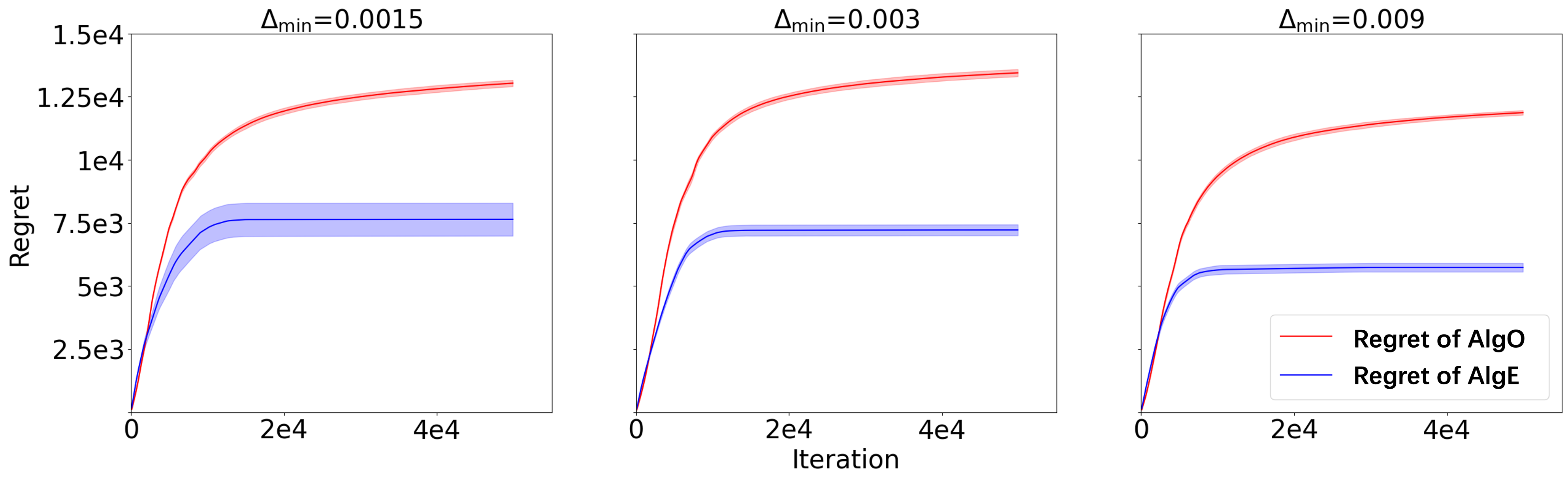
Figure 2: Simulation results with $S=A=H=5$ and different $\Delta_{\min}$, averaged over 10 different random seeds. Error bars show double the standard errors, which correspond to 95% confidence intervals. Our choice of $\text{Alg}^{\text{E}}$ can achieve constant regret as predicted by theory. We can also see the tendency that larger $\Delta_{\min}$ will result in smaller accumulative regret.

References

• Abbasi-Yadkori and Neu [2014] Yasin Abbasi-Yadkori and Gergely Neu. Online learning in mdps with side information. arXiv preprint arXiv:1406.6812, 2014.
• Afsar et al. [2021] M Mehdi Afsar, Trafford Crump, and Behrouz Far. Reinforcement learning based recommender systems: A survey. arXiv preprint arXiv:2101.06286, 2021.
• Auer et al. [2002] Peter Auer, Nicolo Cesa-Bianchi, and Paul Fischer. Finite-time analysis of the multiarmed bandit problem. Machine learning, 47(2):235–256, 2002.
• Avner et al. [2012] Orly Avner, Shie Mannor, and Ohad Shamir. Decoupling exploration and exploitation in multi-armed bandits. arXiv preprint arXiv:1205.2874, 2012.
• Azar et al. [2017] Mohammad Gheshlaghi Azar, Ian Osband, and Rémi Munos. Minimax regret bounds for reinforcement learning. In International Conference on Machine Learning, pages 263–272. PMLR, 2017.
• Buckman et al. [2020] Jacob Buckman, Carles Gelada, and Marc G Bellemare. The importance of pessimism in fixed-dataset policy optimization. arXiv preprint arXiv:2009.06799, 2020.
• Dann et al. [2017] Christoph Dann, Tor Lattimore, and Emma Brunskill. Unifying pac and regret: Uniform pac bounds for episodic reinforcement learning, 2017.
• Dann et al. [2021] Christoph Dann, Teodor Vanislavov Marinov, Mehryar Mohri, and Julian Zimmert. Beyond value-function gaps: Improved instance-dependent regret bounds for episodic reinforcement learning. Advances in Neural Information Processing Systems, 34, 2021.
• Domingues et al. [2021] Omar Darwiche Domingues, Pierre Ménard, Emilie Kaufmann, and Michal Valko. Episodic reinforcement learning in finite mdps: Minimax lower bounds revisited. In Algorithmic Learning Theory, pages 578–598. PMLR, 2021.
• Fujimoto and Gu [2021] Scott Fujimoto and Shixiang Shane Gu. A minimalist approach to offline reinforcement learning. arXiv preprint arXiv:2106.06860, 2021.
• He et al. [2021] Jiafan He, Dongruo Zhou, and Quanquan Gu. Logarithmic regret for reinforcement learning with linear function approximation. In International Conference on Machine Learning, pages 4171–4180. PMLR, 2021.
• Jaksch et al. [2010] Thomas Jaksch, Ronald Ortner, and Peter Auer. Near-optimal regret bounds for reinforcement learning. Journal of Machine Learning Research, 11(4), 2010.
• Jin et al. [2018] Chi Jin, Zeyuan Allen-Zhu, Sebastien Bubeck, and Michael I Jordan. Is q-learning provably efficient? arXiv preprint arXiv:1807.03765, 2018.
• Jin et al. [2021] Ying Jin, Zhuoran Yang, and Zhaoran Wang. Is pessimism provably efficient for offline rl? In International Conference on Machine Learning, pages 5084–5096. PMLR, 2021.
• Kumar et al. [2020] Aviral Kumar, Aurick Zhou, George Tucker, and Sergey Levine. Conservative q-learning for offline reinforcement learning. arXiv preprint arXiv:2006.04779, 2020.
• Lattimore and Szepesvári [2020] Tor Lattimore and Csaba Szepesvári. Bandit algorithms. Cambridge University Press, 2020.
• Levine et al. [2020] Sergey Levine, Aviral Kumar, George Tucker, and Justin Fu. Offline reinforcement learning: Tutorial, review, and perspectives on open problems. arXiv preprint arXiv:2005.01643, 2020.
• Lipsky and Sharp [2001] Martin S Lipsky and Lisa K Sharp. From idea to market: the drug approval process. The Journal of the American Board of Family Practice, 14(5):362–367, 2001.
• Liu et al. [2018] Qiang Liu, Lihong Li, Ziyang Tang, and Dengyong Zhou. Breaking the curse of horizon: Infinite-horizon off-policy estimation. Advances in Neural Information Processing Systems, 31, 2018.
• Liu et al. [2020] Yao Liu, Adith Swaminathan, Alekh Agarwal, and Emma Brunskill. Provably good batch reinforcement learning without great exploration. arXiv preprint arXiv:2007.08202, 2020.
• Modi et al. [2018] Aditya Modi, Nan Jiang, Satinder Singh, and Ambuj Tewari. Markov decision processes with continuous side information. In Algorithmic Learning Theory, pages 597–618. PMLR, 2018.
• Papini et al. [2021] Matteo Papini, Andrea Tirinzoni, Aldo Pacchiano, Marcello Restelli, Alessandro Lazaric, and Matteo Pirotta. Reinforcement learning in linear mdps: Constant regret and representation selection. Advances in Neural Information Processing Systems, 34, 2021.
• Rouyer and Seldin [2020] Chloé Rouyer and Yevgeny Seldin. Tsallis-inf for decoupled exploration and exploitation in multi-armed bandits. In Conference on Learning Theory, pages 3227–3249. PMLR, 2020.
• Simchowitz and Jamieson [2019] Max Simchowitz and Kevin G Jamieson. Non-asymptotic gap-dependent regret bounds for tabular mdps. Advances in Neural Information Processing Systems, 32:1153–1162, 2019.
• Slivkins [2019] Aleksandrs Slivkins. Introduction to multi-armed bandits. arXiv preprint arXiv:1904.07272, 2019.
• Uehara and Sun [2022] Masatoshi Uehara and Wen Sun. Pessimistic model-based offline reinforcement learning under partial coverage. In International Conference on Learning Representations, 2022. URL https://openreview.net/forum?id=tyrJsbKAe6.
• Xie et al. [2021] Tengyang Xie, Ching-An Cheng, Nan Jiang, Paul Mineiro, and Alekh Agarwal. Bellman-consistent pessimism for offline reinforcement learning. arXiv preprint arXiv:2106.06926, 2021.
• Xu et al. [2021] Haike Xu, Tengyu Ma, and Simon S Du. Fine-grained gap-dependent bounds for tabular mdps via adaptive multi-step bootstrap. arXiv preprint arXiv:2102.04692, 2021.
• Yang et al. [2021] Kunhe Yang, Lin Yang, and Simon Du. Q-learning with logarithmic regret. In International Conference on Artificial Intelligence and Statistics, pages 1576–1584. PMLR, 2021.
• Yin and Wang [2021] Ming Yin and Yu-Xiang Wang. Towards instance-optimal offline reinforcement learning with pessimism. In Thirty-Fifth Conference on Neural Information Processing Systems, 2021.
• Yu et al. [2021] Chao Yu, Jiming Liu, Shamim Nemati, and Guosheng Yin. Reinforcement learning in healthcare: A survey. ACM Computing Surveys (CSUR), 55(1):1–36, 2021.
• Yu et al. [2020] Tianhe Yu, Garrett Thomas, Lantao Yu, Stefano Ermon, James Y Zou, Sergey Levine, Chelsea Finn, and Tengyu Ma. Mopo: Model-based offline policy optimization. Advances in Neural Information Processing Systems, 33:14129–14142, 2020.
• Zanette and Brunskill [2019] Andrea Zanette and Emma Brunskill. Tighter problem-dependent regret bounds in reinforcement learning without domain knowledge using value function bounds. In International Conference on Machine Learning, pages 7304–7312. PMLR, 2019.