Spectral lines in FUV and EUV for diagnosing coronal magnetic field

1 Introduction

Sec:Intro The dominance of the magnetic field in the complex structuring of the solar corona is on account of the low plasma $\beta$ (the ratio of kinetic pressure to magnetic pressure). There is a rapid decrease in plasma $\beta$ while going from photosphere to corona due to which the equilibrium field becomes force-free in the corona where magnetic pressure dominates over gas pressure (Priest and Hood, 1991). These magnetic fields play a fundamental role in the formation and evolution of coronal features like coronal loops and streamers, in governing thermal and magnetohydrodynamic (MHD) characteristics of the corona, which in turn regulate the phenomena such as plasma heating, particle acceleration and explosive events. The coronal magnetic fields drive most of the solar events such as flares, jets, coronal mass ejections (CMEs) and solar energetic particles. Information on magnetic field vector and its dynamic evolution is required in the solar atmosphere, more crucially in corona, to understand the exact role it plays in driving these events.

Routine magnetic field measurements are being carried out in the photosphere with high spatial resolution over a selected region of interest as well as over full disk with moderate resolution (Lagg et al., 2017). In the recent past, significant progress has been made with magnetic field measurements in the chromosphere as well (Trujillo Bueno, 2014; Lagg et al., 2017; Ishikawa et al., 2021). On the other hand, coronal magnetic field measurements are still sporadic. Confirmed detection of Stokes $V$ signal through Zeeman effect in the forbidden line due to Fe xiii at 10747 Å had been reported by Lin, Penn, and Tomczyk (2000) and Lin, Kuhn, and Coulter (2004). Raouafi, Lemaire, and Sahal-Bréchot (1999) reported the linear polarization signal in O vi at 1032 Å from the Solar and Heliospheric Observatory (SOHO)/Solar Ultraviolet Measurements of Emitted Radiation (SUMER) spectroscopic observations that was recorded during the roll manoeuver of the SOHO satellite. Raouafi, Lemaire, and Sahal-Bréchot (1999); Raouafi et al. (2002); Raouafi, Sahal-Bréchot, and Lemaire (2002) interpreted this signal in terms of Hanle effect and derived a field strength of $\approx 3$ G at 0.3 $R_{\odot}$ above a coronal hole. The Coronal Multi-channel Polarimeter (CoMP) produced full Stokes spectropolarimetric measurements in coronal emission lines due to Fe xiii at 10747 Å and 10798 Å and, chromospheric line He i at 10830 Å (Tomczyk et al., 2008). In spite of full Stokes spectropolarimetry, the measurements had been mainly used to study magnetic topology in line-of-sight (LOS) aligned structures such as, pseudostreamers (Gibson et al., 2017) and coronal cavities (Ba̧k-Stȩślicka et al., 2013) and, to detect waves for deducing transverse component of the magnetic field (McIntosh et al., 2011; Yang et al., 2020). In near future, high resolution and high precision spectropolarimetric observations from Daniel K. Inouye Solar Telescope (DKIST) may become available for coronal magnetometry, over the wavelength range of 3800 to 50000 Å (Rast et al., 2021). ADITYA-L1, a space based observatory which is expected to be launched in near future, is also expected to produce spectropolarimetric observations of corona in Fe xiii 10747 Å line (Raghavendra Prasad et al., 2017; Nagaraju et al., 2021). Another upcoming ground-based facility is the COronal Solar Magnetism Observatory (COSMO) which will comprise of the Large Coronagraph (LC), the K-coronagraph (K-cor) and the Chromospheric and Prominence Magnetometer (ChroMag) for the measurement of magnetic fields and thermodynamic conditions in the chromosphere and corona (Tomczyk et al., 2016). Apart from observations in ultraviolet/visible/infrared wavelengths, magnetic field measurements in radio and microwave wavelengths have also been reported (Peter et al., 2012; Kishore et al., 2015; Mugundhan et al., 2018; Kumari et al., 2019). A novel spectroscopic technique, so called Magnetic-field induced transition (MIT), is being employed recently to infer magnetic field strength in the corona (Li et al., 2016; Landi et al., 2020, 2021; Li et al., 2021).

The comprehension of large number of physical processes taking place in corona requires accurate knowledge about vector magnetic field simultaneously at multiple heights. The coronal field measurements reported above have one or more limitations to infer the vector magnetic field in the corona. The linear polarization signal of forbidden lines is practically insensitive to magnetic field strength, and it can only constrain the field orientation in the plane perpendicular to LOS (field azimuth) (Casini and Judge, 1999) through the saturated Hanle effect. On the other hand, for permitted lines which fall within the regime of the unsaturated Hanle effect, the linear polarization is in theory sensitive to the full vector magnetic field. With both permitted and forbidden coronal emission lines, the LOS component of the field produces circular polarization through longitudinal Zeeman effect; however, the circularly polarized signal induced by the coronal magnetic field is very weak. The measurements by Lin, Kuhn, and Coulter (2004) have shown that the Stokes $V/I$ signal in Fe xiii at 10747 Å is close to $10^{-4}$ for a LOS field strength of a few Gauss. This signal is expected to be about an order of magnitude smaller in far ultraviolet (FUV) wavelengths for a line with comparable effective Landé factor and line steepness (i.e. $\frac{dI}{d\lambda}$). Owing to wavelength scaling of the Stokes $V/I$ signal, its amplitude will be even smaller at extreme ultraviolet (EUV) wavelengths. Given the difficulties in measuring such low signals, the unsaturated Hanle effect offers a clear advantage as full vector field diagnostic. Bommier, Sahal-Brechot, and Leroy (1981) proposed a method which utilises a minimum of two permitted lines with different Hanle sensitivity to obtain the vector magnetic field information. This method has successfully been applied to derive vector magnetic field in the prominences (Bommier et al., 1994; Bommier, Leroy, and Sahal-Bréchot, 2021), but can in principle be extended to the study of coronal fields. Spectral lines in UV (FUV and EUV) may be best suited to infer the coronal magnetic field vector since, there are several permitted lines located in these wavelength ranges which exhibit varied Hanle sensitivity.

Another advantage of UV lines is that both off-limb as well as on-disk measurements can be carried out at these shorter wavelengths, whereas only off-limb observations are possible in visible/infrared (vis/IR) wavelengths. On-disk measurements are best suited for deriving magnetic field stratification in the solar atmosphere. An amalgamation of UV lines may be used to infer magnetic field at multiple heights since, there are spectral lines in FUV and EUV which form at different heights all the way from photosphere to corona through chromosphere and transition region. One may also choose to combine on-disk photospheric and chromospheric observations in vis/IR with coronal measurements in UV.

There are several studies dedicated to exploiting the capability of individual spectral lines in FUV and EUV to probe the coronal magnetic field. A chief FUV line that has been extensively studied is the O vi at 1032 Å (Sahal-Brechot, Malinovsky, and Bommier, 1986; Raouafi et al., 2002; Raouafi, Sahal-Bréchot, and Lemaire, 2002; Trujillo Bueno, Landi Degl’Innocenti, and Belluzzi, 2017; Zhao et al., 2019). Another FUV line which has been even more extensively studied is the Ly-$\alpha$ at 1216 Å  (Bommier and Sahal-Brechot, 1982; Trujillo Bueno, 2014; Kano et al., 2017, 2019; Hebbur Dayananda et al., 2021). Nevertheless, multiple line diagnostics will provide redundancy which, of course, will help in overcoming the uncertainties and ambiguities in the vector field measurement. There are only a few papers dedicated to such studies. For example, Sahal-Brechot (1981) has given a table of spectral lines consisting of both FUV lines and low temperature IR lines which form either in upper chromosphere or transition region. Judge (1998) has provided a list of forbidden lines in the infrared which are potential diagnostics for probing coronal magnetic field. The current paper is about searching for spectral lines and their combination in FUV and EUV to probe vector magnetic field in the solar corona. The line combinations are chosen such that their formation temperatures are comparable since, it is most likely that they would be originating from the same coronal features.

2 FUV and EUV Spectral Lines and their magnetic sensitivity

Diagnostic capabilities of spectral lines in FUV and EUV in terms of Hanle and Zeeman effects are quantified in this section. Essence of Hanle effect in diagnosing the magnetic field is the modification of scattering polarization (i.e., linear polarization) in spectral lines and rotation of plane of polarization in the presence of external magnetic field. Such an effect is observed when the splitting of energy levels of a given spectral line due to external magnetic field is comparable to their natural broadening. This implies that the Hanle effect is most effective when (Bommier, Sahal-Brechot, and Leroy, 1981)

$$\ilabel{eq:HE_{c}ond1}g_{u}\omega_{B}\tau=1,$$ (1)

where $g_{u}$ is the Landé factor of the upper atomic level; $\omega_{B}$ is the Larmor frequency and $\tau$ is the lifetime of the upper energy level, which is equivalent to the reciprocal of summation over the Einstein $A$ coefficients, assuming that radiation and collision induced transitions are negligible with respect to the spontaneous radiative de-excitation.

The Larmor frequency for a given magnetic field strength $B$ is given by

$$\ilabel{eq:Lm_{f}req}\omega_{B}=\frac{\mu_{B}}{\hbar}B,$$ (2)

where $\mu_{B}$ is Bohr magneton; and $\hbar$ is the reduced Planck constant. When eq. eq:HE_cond1 is satisfied, the corresponding field strength is called the critical field (B_H). Bommier, Sahal-Brechot, and Leroy (1981) have defined the domain of Hanle sensitivity as

$$0.1\leq g_{u}\omega_{B}\tau\leq 10\ilabel{eq:HE_{c}ond2}$$ (3)

based on the uncertainty analysis of vector field determination. In the lower limit, the relative error on field strength is small but uncertainty in determining the field direction is large. In the upper limit, it is the vice-versa. The condition eq:HE_cond2 is further restricted to the domain (Trujillo Bueno, 2014)

$$0.1\leq g_{u}\omega_{B}\tau\leq 5\ilabel{eq:HE_{c}ond3}$$ (4)

which is used in the current work for the selection of suitable spectral lines with varied Hanle sensitivity.

Zeeman effect is caused by the splitting of the energy levels in the presence of external magnetic field which produces characteristic polarization depending on the orientation of vector magnetic field with respect to the observer’s LOS. Given the expected field strength in the corona, permitted lines are mostly in the Hanle regime due to their shorter lifetimes (in the order of 10^-8 s). On the other hand, magnetic sub-levels of the forbidden lines are well separated (i.e., $g_{u}\omega_{B}\tau\gg 5$, which breaks the condition eq:HE_cond3). As a consequence, only the LOS field strength through circular polarization (Harvey, 1969) and the field azimuth through linear polarization (Querfeld and Smartt, 1984; Arnaud and Newkirk, 1987) can be determined from these lines. This is because the linear polarization produced by the transverse Zeeman effect is below the detection level of current observational capabilities for magnetic fields of a few Gauss. Thus, Stokes $Q$ and $U$ are completely dominated by the residual atomic alignment which does not depend on the field strength (so-called saturated Hanle effect: Sahal-Brechot (1977)). The circular polarization (i.e. Stokes $V$) is also weak but a few measurements had been reported in the literature. For example, the observations carried out by Lin, Penn, and Tomczyk (2000) and Lin, Kuhn, and Coulter (2004) had shown the Stokes $V$ amplitudes in the order of $10^{-4}$ for the longitudinal field strength of a few Gauss. The observations were carried out in Fe xiii line at 10747 Å. For the emission lines in FUV and EUV, this signal is expected to be weaker by at least an order of magnitude because of the way the circular polarization sensitivity index ($s_{V}$) scales with the wavelength given as (same as Eq. 9.88 of Landi Degl’Innocenti and Landolfi (2004), but calculated for an emission line with Gaussian profile)

$$s_{V}=\left(\frac{\lambda_{0}}{\lambda_{\mathrm{ref}}}\right)\overline{g}d_{c},\ilabel{eq:StokesVsensitivity}$$ (5)

where $\lambda_{0}$ is the central wavelength of the emission line under consideration; $\lambda_{\mathrm{ref}}$ is a reference wavelength (e.g., 1242 Å); $\overline{g}$ is the effective Landé factor; and $d_{c}=1-I(\lambda_{0})/I_{c}$, is the line centre depression (negative) with $I_{c}$ being the continuum intensity adjacent to the spectral emission line. The basis for deriving eq. eq:StokesVsensitivity is the equation that relates Stokes $V$ to the longitudinal magnetic field (B_∥) under weak field approximation (Landi Degl’Innocenti and Landolfi, 2004) which is given by

$$\frac{V(\lambda)}{I(\lambda)}=-4.67\times 10^{-13}~{}\overline{g}\lambda^{2}B_{\parallel}\frac{1}{I(\lambda)}\frac{dI(\lambda)}{d\lambda}.\ilabel{eq:Vsignal}$$ (6)

In the above equation $\frac{dI(\lambda)}{d\lambda}$ is the intensity derivative with respect to wavelength. As can be seen from eq. eq:Vsignal, apart from the wavelength dependence, Stokes $V$ amplitude also depends on $\overline{g}$ and $\frac{dI(\lambda)}{d\lambda}$ which usually differ from one spectral line to the other. Hence, it is worth checking for the Stokes $V$ sensitivity of the spectral lines in UV so that this information may be combined with the Hanle measurements to infer the vector magnetic field.

As can be seen from eqs. eq:HE_cond1 to eq:Vsignal, effective Landé factor, Einstein $A$ coefficients and $\frac{dI(\lambda)}{d\lambda}$ corresponding to a given spectral line are some of the essential parameters to determine its magnetic sensitivity. In addition, as spectropolarimetric measurements are in general photon starved, line irradiance is also taken into account while checking for the diagnostic potential of a given spectral line to probe the magnetic field. The estimation or compilation of these parameters is discussed briefly in the following subsections.

2.1 Spectral lines

In this analysis, spectral lines observed from three different space-based missions are compiled. One is the EUV Imaging Spectrometer (EIS; Culhane, 2007), onboard the Hinode spacecraft, which is designed to observe in two wavelength ranges (SW: 166 – 212 Å; LW: 245 – 291 Å). These wavelength bands consist of several emission lines from highly ionised species ranging from 4.7 to 7.3 in the logarithmic scale of temperature (log₁₀(T)). Another is a sounding rocket instrument, named the Extreme Ultraviolet Normal Incidence Spectrograph (EUNIS), which observed a coronal bright point around 18:12 UT on 2006 April 12. A brief description of the instrument has been provided by Brosius, Rabin, and Thomas (2007). The EUV spectra obtained by EUNIS covers first-order wavelengths from 300 to 370 Å over a temperature range of 5.2 to 6.4 in log₁₀(T) (Brosius et al., 2008). The third instrument is SUMER which is a high-resolution telescope and spectrograph, onboard the Solar and Heliospheric Observatory (SOHO), which observed the sun over the wavelength range from 470 to 1609 Å (Curdt and Landi, 2001; Curdt, Landi, and Feldman, 2004).

The spectral lines thus compiled are listed in Table Tab:eff_g. The atomic species along with their ionization state are listed in the first column and the observed wavelength in Angstrom (Å) is given in the second column. In the third column listed are the corresponding level configurations. The fourth and the fifth columns list the peak formation temperature (logarithmic value) of the lines and the transition type, respectively. These line formation temperatures are taken from Feldman et al. (1997); Brosius et al. (2008); Curdt and Landi (2001); Zanna and Mason (2005); Young et al. (2007); Moran (2003). Although the peak formation temperature is mentioned for most of the spectral lines in Table Tab:eff_g, it should be noted that the lines are always formed in a range of temperature, not at a single value (Feldman et al., 1998; Warren and Warshall, 2002; Warren and Brooks, 2009; Saqri et al., 2020). For example, any spectral line shown at $\mathrm{log}_{10}(T)=6.1$ may actually be formed within a range of $\mathrm{log}_{10}(T)=5.85$ to 6.3. Further, the critical field strength (in Gauss) for maximum Hanle sensitivity are listed in the ninth column. The remaining columns are described in the following subsections.

2.2 Transition probability

The lifetime of the upper energy level is equal to the reciprocal of sum over the Einstein $A$ coefficients, i.e. $\tau=\frac{1}{\sum_{j}A_{kj}}$. Transition probability or the Einstein $A$ coefficient ($A=\sum_{j}$ A_kj) is the total rate of all spontaneous radiative transitions from the upper level (k) to all the lower levels to which the level k can de-excite. These coefficients help in determining the range of magnetic field strength to which the spectral lines are sensitive in the Hanle regime (cf. eqs. eq:HE_cond1 and eq:HE_cond2). Besides, they are also important for the visibility of the spectral lines in the solar corona. The $A$ values are obtained from current version 10.0 of the CHIANTI atomic database (Dere et al., 1997; Del Zanna et al., 2021) and are listed in the sixth column of Table Tab:eff_g.

2.3 Landé factors

In light elements, the electrostatic interaction dominates over the spin-orbit coupling such that the orbital angular momenta of the individual electrons get coupled to give a total orbital angular momentum ${\mathbfit L}$, while the spins of the electrons get coupled to give a total spin ${\mathbfit S}$. This is referred to as Russell-Saunders or LS coupling. However, for heavier atoms with larger nuclear charge, the spin-orbit interactions are stronger leading to jj coupling. A more general and practical case exists in certain atoms, particularly mid-weight atoms and those with almost closed shells, which lie in between these two coupling limits. Such a coupling is termed as intermediate or i-coupling, in which both the electrostatic and the spin-orbit interactions may be present with a relative order of magnitude. From the selection rules described in Condon and Shortley (1935) and Drake (2006), the coupling scheme of the atomic levels associated with the dipole (electric or magnetic) transitions are identified. In case of LS coupling, the following expression is used to determine the Landé factors of individual energy levels.

$$g=\frac{3}{2}+\frac{S(S+1)-L(L+1)}{2J(J+1)}\ilabel{eq:g_{L}S}$$ (7)

where $L$ and $S$ are the total orbital and spin angular momentum quantum numbers, respectively; and $J$ is the total angular momentum which is defined as ${\mathbfit J}={\mathbfit L}+{\mathbfit S}$. Equation eq:g_LS holds only for LS coupling scheme which may fail in cases involving atomic or ionic lines of high excitation potential and intermediate coupling may have to be considered. There are no lines exhibiting jj coupling in this analysis. For intermediate coupling, the Landé factors $g_{1}$ and $g_{2}$ are first estimated using formula eq:g_LS and then compared with the values (for those available) from Verdebout et al. (2014). It is found that the values calculated in this work match closely with those estimated using the GRASP2K (Jönsson et al., 2007) code in Verdebout et al. (2014). GRASP2K is a fully relativistic multiconfiguration Dirac-Hartree-Fock (MCDHF) method based atomic structure package. The Landé factors of the individual levels are listed in the seventh column of Table Tab:eff_g.

The effective Landé factors are calculated using the following formula (Landi Degl’Innocenti, 1982).

$$\overline{g}=\frac{1}{2}(g_{1}+g_{2})+\frac{1}{4}(g_{1}-g_{2})[J_{1}(J_{1}+1)-J_{2}(J_{2}+1)]\ilabel{eq:g}$$ (8)

where $J_{1}$ and $g_{1}$ are the total angular momentum and Landé factor of the lower energy level, respectively; $J_{2}$ and $g_{2}$ correspond to that of the upper energy level. All the estimated values of $\overline{g}$ factor are listed in the eighth column of Table Tab:eff_g.

2.4 Polarizability coefficient

The polarizability coefficient ($W_{2}$) is a scaling factor which quantifies the fraction of linear polarization produced by resonant scattering of the incoming radiation. Analytical expressions for $W_{2}$ for three allowed transitions corresponding to $\Delta J=J_{2}-J_{1}=0,\pm 1$ (with $J_{2}=J_{1}=0$ being forbidden) are given by (Stenflo, 1994)

Case I: When $J_{2}=J_{1}-1$,

$$\ilabel{eq:C1}W_{2}=\frac{(J_{1}-1)(2J_{1}-3)}{10J_{1}(2J_{1}+1)}$$ (9)

Case II: When $J_{2}=J_{1}$,

$$\ilabel{eq:C2}W_{2}=\frac{(2J_{1}-1)(2J_{1}+3)}{10J_{1}(J_{1}+1)}$$ (10)

Case III: When $J_{2}=J_{1}+1$,

$$\ilabel{eq:C3}W_{2}=\frac{(J_{1}+2)(2J_{1}+5)}{10(J_{1}+1)(2J_{1}+1)}$$ (11)

The calculated values of $W_{2}$ for the corresponding UV spectral lines are listed in the tenth column of Table Tab:eff_g.

2.5 Line irradiance

For this work, only the coronal lines are focused on. The EIS off-limb spectra consists of spectral lines whose intensities over active region and quiet sun have been collected from Del Zanna (2012). The off-limb line intensities from 470 to 1609 Å spanning over three regions (quiet sun (QS), active region (AR) and coronal hole (CH)) have been assembled from Curdt, Landi, and Feldman (2004). All the line irradiances from EIS and SUMER are available in the units of photons cm^-2 s^-1 arcsec^-2. But for the EUNIS on-disk observations of spectral lines from 300 to 370 Å, the given line irradiances are converted from erg cm^-2 s^-1 sr^-1 to photons cm^-2 s^-1 arcsec^-2 (formula eq:int_co) in order to simplify the comparison with other spectral lines (from EIS and SUMER observations) used in the present analysis. The spectral irradiances for different solar regions, where available, are listed in Table Tab:eff_g in the units of photons cm^-2s^-1arcsec^-2.

$$\ilabel{eq:int_{c}o}1~{}erg~{}cm^{-2}s^{-1}sr^{-1}=11.8324\times 10^{-4}\times\lambda~{}photons~{}cm^{-2}s^{-1}arcsec^{-2}$$ (12)

where, $\lambda$ is the wavelength (in Å) of the corresponding spectral line.

2.6 Intensity derivative

In the context of inferring vector magnetic field in the corona, the expected amplitude of Stokes $V$ profiles of a few selected UV lines have been estimated in this work. In addition to the effective Landé factor and the wavelength, the Stokes $V$ signal also depends on the intensity derivative $\frac{dI}{d\lambda}$ (cf. equation eq:Vsignal). The spectroscopic observations from SUMER (for details, refer to Curdt and Landi, 2001; Curdt, Landi, and Feldman, 2004) are used for selecting the spectral lines. Relevant data have been downloaded from https://sdac.virtualsolar.org.

 

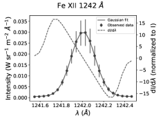
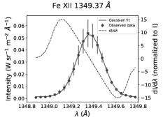
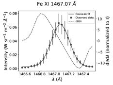
Figure 1.: Sample intensity profiles of Fe xii at 1242 Å(the left panel) and 1349 Å(the middle panel), and Fe xi at 1467 Å(the right panel) are shown along with their corresponding derivative plots. The solid curves are the Gaussian fit to the observed data points (the filled circles). The error bars correspond to the dispersion in intensity values across the spatial pixels over which the spectral profiles are averaged. The dotted curves are the derivative of the fitted Gaussian curves normalized to the local intensities.Fig:Int˙prof

Before estimating the intensity derivative, the spectral profiles corresponding to a given spectral line are fitted with Gaussian function. The derivatives of intensity with respect to wavelength are calculated and normalized to the local intensity of each Gaussian fitted profile. Then the derivative values (absolute and normalized) at half-maxima of both the blue and the red wings are averaged using which the Stokes $V/I$ amplitude is estimated for each Gaussian fitted profile along the spatial axis via equation eq:Vsignal. Finally, the mean Stokes $V/I$ amplitude is calculated for the given spectral line. The standard deviation of the Stokes $V/I$ amplitude is also estimated relative to its mean value over the fitted spectral profiles. In the above analysis, the Stokes $V/I$ amplitude increases by 1.3 (for detector A) and 1.1 (for detector B) when the Stokes I profiles are corrected for the instrumental broadening. This implies that there is no significant change in the Stokes $V/I$ amplitudes due to instrumental broadening effect and therefore while calculating Stokes $V/I$, it can safely be unaccounted for.

Figure Fig:Int_prof shows the sample mean intensity profiles of a few selected forbidden lines in FUV due to Fe xii at 1242 Å (the left panel), 1349 Å (the middle panel), and Fe xi at 1467 Å (the right panel) along with their corresponding mean intensity derivatives (the dotted curves). The error bars correspond to the dispersion in intensity values across the spatial pixels over which the spectral profiles are averaged. For a LOS field of 10 Gauss, the expected Stokes $V/I$ amplitudes for Fe xii lines at 1242 Å and 1349 Å are $(1.22\pm 0.096)\times 10^{-4}$ and $(1.95\pm 0.069)\times 10^{-4}$, respectively, and for Fe xi line at 1467 Å, is $(1.34\pm 0.11)\times 10^{-4}$. Similar calculations have been done for spectral lines below 1200 Å and we found that the Stokes $V/I$ signal is in the order of 10^-5 or less.

3 Summary and Conclusion

Sec:Res_Disc

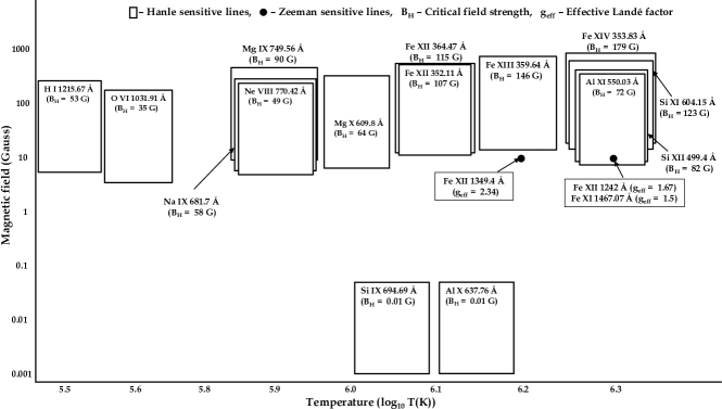
Figure 2.: Graphical representation of magnetic sensitivity of the spectral lines in the domain of Hanle effect (cf. Eq. eq:HE_cond3). The domains are shown in rectangular boxes, each of which covers an approximate temperature range along the X-axis and, magnetic field strength from 0.1B_H to 5B_H along the Y-axis (Not to be scaled). The middle of each rectangular box along the X-axis respresents the peak line formation temperature. FUV spectral lines, having best estimated Stokes $V$ signal, are shown using solid circles at a coronal field of 10 G.fig:Hanle˙Zee˙sens

The search for spectral lines in FUV and EUV to probe vector magnetic field has been carried out in this paper. The outcome of this search is summarized in a graphical representation shown in Figure fig:Hanle_Zee_sens. In this figure each line is represented by a rectangular box with its length along Y-axis indicating the magnetic field sensitivity range due to Hanle effect as dictated by Eq. eq:HE_cond3. The width of the box along X-axis is not a true representation of temperature sensitivity range but only to indicate the peak formation temperature given in logarithmic scale. Actual temperature sensitivity extends much beyond that is indicated by the width of the box. Each box is marked by the wavelength of the spectral line along with the corresponding name of the ion and Hanle critical magnetic field ($B_{H}$). The closed solid circles in this figure represent the FUV lines shown in Figure Fig:Int_prof. Their locations in Figure fig:Hanle_Zee_sens indicate the peak formation temperature on the X-axis and the assumed field strength of 10 Gauss, at which their Stokes $V/I$ signal is expected to be in the order of $10^{-4}$, on the Y-axis. For estimation of Stokes $V/I$ signal, Eq. eq:Vsignal is used along with the measured intensity derivative ($\frac{dI}{d\lambda}$). While selecting the spectral lines presented in Figure fig:Hanle_Zee_sens, the polarizability coefficient ($W_{2}$), line irradiance and $B_{H}$ are considered. Only lines with $B_{H}$ in the range 0.01 - 200 G, $W_{2}>0$ and their intensity $>$ 1 photon cm^-2s^-1arcsec^-2 are shown in Figure fig:Hanle_Zee_sens. The range of field strength chosen is directed by the coronal magnetic field measurements reported in the literature (see for e.g., Fig 5. of Peter et al., 2012 and Figure 4. of Sasikumar Raja et al., 2021).

Regarding the intensity criteria, it is apparent that the spectral lines with maximum irradiance should be chosen as, spectropolarimetric observations are photon starved. However, it is difficult to find spectral lines with high irradiance which are sensitive to Hanle and Zeeman effects and, cover a suitable temperature range as well. The O vi line at 1031.91 Å is a good Hanle sensitive line both in terms of number of photons and $B_{H}$. However, in order to derive vector magnetic field there is no other spectral line with the same peak formation temperature. Given the fact that the line formation temperature is not a delta function but has a range, this line can be used with other lines having adjacent formation temperature. For instance, this line can be used together with Ne viii at 770.42 Å to derive vector magnetic field information. Though the number of photons in these two lines are relatively close, they are separated in their wavelengths by $\approx 260$ Å and formation temperature differs by $\approx 0.3$ on logarithmic scale. Similarly, Ly-$\alpha$ line at 1215.67 Å is sensitive to Hanle effect (B_H= 53 G) having extremely high line irradiance. However, there is no spectral line with similar line irradiance and formation temperature to be used in association with Ly-$\alpha$.

The O vi at 1037.61 Å and Ne viii at 780.39 Å lines with $W_{2}=0$ can be used for zero polarization reference which may help in correcting for systematic artifacts. The Na ix at 681.72 Å can also be used together with Ne viii at 770.42 Å but the number of photons is significantly less (close to a factor of 4). The combination of Ne viii at 770.42 Å ($\mathrm{log}_{10}(T)=5.9$, $B_{H}=49$ G) and Mg x at 609.79 Å ($\mathrm{log}_{10}(T)=6.0$, $B_{H}=64$ G) is good to probe vector magnetic field from the regions of plasma with temperature in the range $\mathrm{log}_{10}(T)=5.9-6.0$. Both lines have good line irradiance. However, the wavelength separation is about 160 Å between these two lines. Nevertheless, with this line combination also there are two spectral lines viz., Ne viii at 780.39 Å and Mg x at 624.94 Å, which can be used as zero polarization reference. Interestingly, Si ix at 694.69 Å has similar line irradiance as Na ix at 681.72 Å and exhibit different sensitivity to Hanle effect, with ${g_{u}}\omega_{B}\tau=$ 1 for 0.01 G and 58 G, respectively. Therefore, Si ix 694.69 Å line will be principally sensitive to the field direction, while Na ix 681.72 Å will be suited for determining the magnetic field strength.

There are several spectral lines in the wavelength range of 350 - 370 Å with B${}_{H}=100-180$ G which can be used to probe vector field from the regions with plasma temperature of $\mathrm{log}_{10}(T)=$ 6.1 to 6.3. The greatest advantage here is that these lines are clustered within a wavelength band of about 20 Å which is beneficial in terms of instrument design and development. However, these lines have moderate number of photons compared to the lower temperature lines mentioned in the preceding paragraphs. At $\mathrm{log}_{10}(T)=6.3$ there are two spectral lines which are best suited for vector magnetic field measurements viz., Al xi at 550 Å and Si xii at 499.4 Å both in terms of their wavelength proximity and $B_{H}$ values which are 72 G and 82 G, respectively.

Some of the Hanle saturated lines in FUV are also explored in the context of providing additional constraints on the LOS component of the magnetic field vector. However, their wavelength separation is larger, with respect to Hanle sensitive lines of identical formation temperatures, making them less attractive for vector magnetic field measurements (cf. Figure fig:Hanle_Zee_sens). Hence the spectral lines with different Hanle sensitivity are best suited for probing vector magnetic field in the solar corona, at least in the temperature range of $\mathrm{log}_{10}(T)=5.5-6.3$. The Hanle sensitivity of the spectral lines given in Figure fig:Hanle_Zee_sens is limited to $\geq 4$ Gauss, with the exception of Si ix and Al x lines having Hanle sensitivity from 0.001 to 0.05 Gauss which may be useful in probing very weak magnetic field in the milliGauss range. This implies that the coronal height up to which most of the magnetic field measurements can be carried out is limited to $<2$ R_⊙. At this range of height, the impact of electron collisions becomes significant due to larger electron density and one of its main effect is depolarization. In order to estimate the depolarization factor due to collisions, it is important to calculate and compare between the collisional and the radiative rates through detailed modeling of each individual line shown in Figure fig:Hanle_Zee_sens. Therefore, depolarizing collisions along with other symmetry breaking processes such as non-radial solar wind, ion temperature anisotropy and presence of active regions (Fineschi et al., 1993; Zhao et al., 2019, 2021) must be taken into account while interpreting the spectropolarimetric information in actual observations.

Table 1.: Table showing ionization state of the atomic species, corresponding wavelength and level configuration, temperature of line formation (log₁₀(T)), type of transition (TT: E1 or M1), effective Landé factor ($\overline{g}$) , critical field strength (B_H), polarizability coefficient (W₂) and line irradiances in three different solar regions. E1 and M1 refer to electric dipole and magnetic dipole transitions, respectively. ^2S+1L_J is the notation used in each atomic level configuration, where L, S and J are total orbital, spin and angular momentum quantum numbers respectively.Tab:eff˙g

Ion $\lambda$(Å) Transition (i-k) log₁₀(T) TT $A(s^{-1})$ $\bf{g_{i}-g_{k}}$ $\bf{\overline{g}}$ B_H W₂ L (ph cm^-2s^-1arcsec^-2) (Gauss) QS AR CH Fe IX 171.073 3s² 3p^{6 1}S₀ 6.11 E1 $2.28\times 10^{11}$ 1 - 1 1 25817 1 140.7 265 - - 3s² 3p⁵ 3d ¹P₁ Fe X 174.531 3s² 3p^{5 2}P_3/2 6 E1 $1.86\times 10^{11}$ 1.33-1.2 1.1 17551 0.28 119.7 172.7 - - 3s² 3p⁴ 3d ²D_5/2 Fe X 184.537 3s² 3p^{5 2}P_3/2 6 E1 $1.63\times 10^{11}$ 1.33 - 2 1.17 9245 0 33.6 47.9 - - 3s² 3p⁴ 3d ²S_1/2 Fe XII 195.119 3s² 3p^{3 4}S_3/2 6.1 E1 $8.83\times 10^{10}$ 2 - 1.6 1.3 6249 0.28 136.2 312 - - 3s² 3p² 3d ⁴P_5/2 Fe XIII 202.044 3s² 3p^{2 3}P₀ 6.2 E1 $5.33\times 10^{10}$ 1.5 - 1.5 1.5 4024 1 103.3 349.5 - - 3s² 3p 3d ³P₁ Si X 258.374 2s² 2p ²P_3/2 6.1 E1 $1.72\times 10^{10}$ 1.33-1.33 1.33 1461 0.32 44.1 66.3 - - 2s 2p^{2 2}P_3/2 Si X 261.056 2s² 2p ²P_3/2 6.1 E1 $1.68\times 10^{10}$ 1.33-0.67 1.5 2853 0 26.3 37.8 - - 2s 2p^{2 2}P_1/2 Fe XIV 264.788 3s² 3p ²P_3/2 6.3 E1 $4.26\times 10^{10}$ 1.33-1.33 1.33 3618 0.32 17.1 92.1 - - 3s 3p^{2 2}P_3/2 Fe XV 284.163 3s^{2 1}S₀ 6.3 E1 $2.11\times 10^{10}$ 1 - 1 1 2389 1 24.3 576.6 - - 3s 3p ¹P₁ Si XI 303.325 1s² 2s^{2 1}S₀ 6.2 E1 $6.38\times 10^{9}$ 1 - 1 1 722 1 - 1049 - - 1s² 2s 2p ¹P₁ Fe XI 308.544 3s² 3p^{4 1}D₂ 6.1 E1 $8.84\times 10^{9}$ 1 - 1 1 1001 0.01 - 13 - - 3s 3p^{5 1}P₁ Fe XIII 312.174 3s² 3p^{2 3}P₁ 6.2 E1 $4.07\times 10^{9}$ 1.5 - 1.5 1.5 307 0.25 - 12 - - 3s 3p^{3 3}P₁

Ion $\lambda$(Å) Transition (i-k) log₁₀(T) TT $A(s^{-1})$ $\bf{g_{i}-g_{k}}$ $\bf{\overline{g}}$ B_H W₂ L (ph cm^-2s^-1arcsec^-2) (Gauss) QS AR CH Fe XIII 318.13 3s² 3p^{2 1}D₂ 6.2 E1 $5.61\times 10^{9}$ 1 - 1 1 635 0.35 - 10.8 - - 3s 3p^{3 1}D₂ Fe XIII 320.8 3s² 3p^{2 3}P₂ 6.2 E1 $3.89\times 10^{9}$ 1.5 - 1.5 1.5 294 0.35 - 40.4 - - 3s 3p^{3 3}P₂ Fe XV 327.033 3s 3p ³P₂ 6.3 E1 $4.67\times 10^{9}$ 1.5 - 1 1.25 529 0.35 - 6.4 - - 3p^{2 1}D₂ Cr XIII 328.268 2p⁶ 3s^{2 1}S₀ 6.2 E1 $1.73\times 10^{10}$ 1 - 1 1 1959 1 - 25 - - 3s 3p ¹P₁ Al X 332.79 1s² 2s^{2 1}S₀ 6.1 E1 $5.74\times 10^{9}$ 1 - 1 1 650 1 - 35.2 - - 1s² 2s 2p ¹P₁ Fe XIV 334.178 3s² 3p ²P_1/2 6.3 E1 $2.49\times 10^{9}$ 0.67 - 0.8 0.83 352 0.5 - 74 - - 3s 3p^{2 2}D_3/2 Fe XVI 335.409 2p⁶ 3s ²S_1/2 6.4 E1 $7.87\times 10^{9}$ 2 - 1.33 1.17 669 0.5 - 159 - - 2p⁶ 3p ²P_3/2 Fe XII 338.263 3s² 3p^{3 2}D_5/2 6.1 E1 $3.37\times 10^{9}$ 1.2 - 1.2 1.2 318 0.37 - 23.8 - - 3s 3p^{4 2}D_5/2 Fe XI 341.113 3s² 3p^{4 3}P₂ 6.1 E1 $3.28\times 10^{9}$ 1.5 - 1.5 1.5 248 0.01 - 25.5 - - 3s 3p^{5 3}P₁ Si IX 341.949 2s² 2p^{2 3}P₀ 6.1 E1 $2.4\times 10^{9}$ 1.5 - 0.5 1 544 1 - 18.2 - - 2s 2p^{3 3}D₁ Fe XII 346.852 3s² 3p^{3 4}S_3/2 6.1 E1 $1.86\times 10^{9}$ 2 - 2.67 1.83 - 0 - 30.2 - - 3s 3p^{4 4}P_1/2 Fe XIII 348.183 3s² 3p^{2 3}P₀ 6.2 E1 $1.61\times 10^{9}$ 1.5 - 0.5 1 365 1 - 29.3 - - 3s 3p^{3 3}D₁ Fe XII 352.106 3s² 3p^{3 4}S_3/2 6.1 E1 $1.64\times 10^{9}$ 2 - 1.73 1.87 107 0.32 - 64.8 - - 3s 3p^{4 4}P_3/2

Ion $\lambda$(Å) Transition (i-k) log₁₀(T) TT $A(s^{-1})$ $\bf{g_{i}-g_{k}}$ $\bf{\overline{g}}$ B_H W₂ L (ph cm^-2s^-1arcsec^-2) (Gauss) QS AR CH Fe XI 352.67 3s² 3p^{4 3}P₂ 6.1 E1 $3.11\times 10^{9}$ 1.5 - 1.5 1.5 235 0.35 - 64.3 - - 3s 3p^{5 3}P₂ Fe XIV 353.829 3s² 3p ²P_3/2 6.3 E1 $1.9\times 10^{9}$ 1.33 - 1.2 1.1 179 0.28 - 38.6 - - 3s 3p^{2 2}D_5/2 Fe XI 356.519 3s² 3p^{4 3}P₁ 6.1 E1 $3.28\times 10^{9}$ 1.5 - 1.5 1.5 248 0.25 - 10.4 - - 3s 3p^{5 3}P₁ Fe XIII 359.644 3s² 3p^{2 3}P₁ 6.2 E1 $1.5\times 10^{9}$ 1.5 - 1.17 1 146 0.35 - 54.1 - - 3s 3p^{3 3}D₂ Fe XIII 359.839 3s² 3p^{2 3}P₁ 6.2 E1 $1.61\times 10^{9}$ 1.5 - 0.5 1 365 0.25 - 5.3 - - 3s 3p^{3 3}D₁ Fe XVI 360.758 2p⁶ 3s ²S_1/2 6.4 E1 $6.34\times 10^{9}$ 2 - 0.67 1.33 - 0 - 76.9 - - 2p⁶ 3p ²P_1/2 Fe XII 364.467 3s² 3p^{3 4}S_3/2 6.1 E1 $1.62\times 10^{9}$ 2 - 1.6 1.33 115 0.28 - 85.4 - - 3s 3p^{4 4}P_5/2 Mg IX 368.071 1s² 2s^{2 1}S₀ 6.0 E1 $5.12\times 10^{9}$ 1 - 1 1 580 1 - 486 - - 1s² 2s 2p ¹P₁ Fe XI 369.163 3s² 3p^{4 3}P₁ 6.1 E1 $3.11\times 10^{9}$ 1.5 - 1.5 1.5 235 0.35 - 20.5 - - 3s 3p^{5 3}P₂ Si XII 499.4 1s² 2s ²S_1/2 6.3 E1 $9.61\times 10^{8}$ 2 - 1.33 1.17 82 0.5 23.3 166.4 - - 1s² 2p ²P_3/2 Si XII 520.67 1s² 2s ²S_1/2 6.26 E1 $8.48\times 10^{8}$ 2 - 0.67 1.33 - 0 13.3 100.9 - - 1s² 2p ²P_1/2 Al XI 550.031 1s² 2s ²S_1/2 6.26 E1 $8.52\times 10^{8}$ 2 - 1.33 1.17 72 0.5 7.9 48.5 - - 1s² 2p ²P_3/2 Ca X 557.76 2p⁶ 3s ²S_1/2 5.85 – 6 E1 $3.77\times 10^{9}$ 2 - 1.33 1.17 320 0.5 9.0 19.7 5.2 - 2p⁶ 3p ²P_3/2

Ion $\lambda$(Å) Transition (i-k) log₁₀(T) TT $A(s^{-1})$ $\bf{g_{i}-g_{k}}$ $\bf{\overline{g}}$ B_H W₂ L (ph cm^-2s^-1arcsec^-2) (Gauss) QS AR CH Al XI 568.12 1s² 2s ²S_1/2 6.26 E1 $7.73\times 10^{8}$ 2 - 0.67 1.33 - 0 5.3 23.5 - - 1s² 2p ²P_1/2 Ca X 574.01 2p⁶ 3s ²S_1/2 5.85 – 6 E1 $3.47\times 10^{9}$ 2 - 0.67 1.33 - 0 6.0 12.2 3.2 - 2p⁶ 3p ²P_1/2 Si XI 604.15 2s 2p ¹P₁ 6.26 E1 $1.09\times 10^{9}$ 1 - 1 1 123 0.35 2.5 4.1 - - 2p^{2 1}D₂ Mg X 609.793 1s² 2s ²S_1/2 6.04 E1 $7.53\times 10^{8}$ 2 - 1.33 1.17 64 0.5 213 341 26 - 1s² 2p ²P_3/2 Mg X 624.94 1s² 2s ²S_1/2 6 E1 $7\times 10^{8}$ 2 - 0.67 1.33 - 0 118 346 16 - 1s² 2p ²P_1/2 Al X 637.763 2s^{2 1}S₀ 6.15 E1 $1.94\times 10^{5}$ 1 - 1.5^* 1.5 0.01 1 3 4.9 0.18 - 2s 2p ³P₁ Al X 670.053 2s 2p ¹P₁ 6.13 E1 $9.38\times 10^{8}$ 1 - 1 1 106 0.35 0.38 0.61 0.07 – 2p^{2 1}D₂ Si IX 676.503 2s² 2p^{2 3}P₁ 6.05 E1 $6.54\times 10^{4}$ 1.5 - 2^* 2.25 $\ll$ 1 0.35 2.0 2.1 0.63 - 2s 2p^{3 5}S₂ Al IX 680.318 2s² 2p ²P_1/2 6.02 E1 $3.75\times 10^{4}$ 0.67 - 1.73^* 2 $\ll$ 1 0.5 4.3 4.4 0.33 - 2s 2p^{2 4}P_3/2 Na IX 681.719 1s² 2s ²S_1/2 5.92 E1 $6.78\times 10^{8}$ 2 - 1.33 1.17 58 0.5 7.6 34.6 4.9 - 1s² 2p ²P_3/2 Mg VIII 689.641 2s 2p^{2 2}P_3/2 ^a  5.95 E1 $4.15\times 10^{9}$ 1.33 - 1.2 1.1 392 0.28 0.31 0.76 0.33 - 2p^{3 2}D_5/2 Na IX 694.261 1s² 2s ²S_1/2 5.92 E1 $6.42\times 10^{8}$ 2 - 0.67 1.33 - 0 3.5 18.4 2.6 - 1s² 2p ²P_1/2 a Moran, 2003 * Landé factor of upper and lower energy level has been compared with Verdebout et al. (2014)

Ion $\lambda$(Å) Transition (i-k) log₁₀(T) TT $A(s^{-1})$ $\bf{g_{i}-g_{k}}$ $\bf{\overline{g}}$ B_H W₂ L (ph cm^-2s^-1arcsec^-2) (Gauss) QS AR CH Si IX 694.686 2s² 2p^{2 3}P₂ 6.05 E1 $2.16\times 10^{5}$ 1.5 - 2^* 1.75 0.01 0.35 4.1 6.7 1.5 - 2s 2p^{3 5}S₂ Ar VIII 700.24 2p⁶ 3s ²S_1/2 5.61 E1 $2.7\times 10^{9}$ 2 - 1.33 1.17 229 0.5 1.0 1.3 0.87 - 2p⁶ 3p ²P_3/2 Mg IX 706.06 1s² 2s^{2 1}S₀ 5.99 E1 $9.7\times 10^{4}$ 1 - 1.5^* 1.5 $\ll$ 1 1 10.2 21.5 9.2 - 1s² 2s 2p ³P₁ Ar VIII 713.801 2p⁶ 3s ²S_1/2 5.61 E1 $2.56\times 10^{9}$ 2 - 0.67 1.33 - 0 0.45 0.85 0.51 - 2p⁶ 3p ²P_1/2 Mg IX 749.552 1s² 2s 2p ¹P₁ 5.85–6 E1 $7.96\times 10^{8}$ 1 - 1 1 90 0.35 1.6 4.4 1.6 - 1s² 2p^{2 1}D₂ Mg VIII 762.66 2s² 2p ²P_1/2 5.91 E1 $1.82\times 10^{4}$ 0.67 - 1.73^* 2 $\ll$ 1 0.5 0.1 0.35 0.33 - 2s 2p^{2 4}P_3/2 Mg VIII 769.355 2s² 2p ²P_1/2 5.91 E1 $1.38\times 10^{5}$ 0.67 - 2.67^* 1.67 - 0 0.24 0.97 0.97 - 2s 2p^{2 4}P_1/2 Ne VIII 770.42 1s² 2s ²S_1/2 5.85-6 E1 $5.76\times 10^{8}$ 2 - 1.33 1.17 49 0.5 39.5 177.9 41.4 - 1s² 2p ²P_3/2 Mg VIII 772.26 2s² 2p ²P_3/2 5.91 E1 $6.06\times 10^{4}$ 1.33 - 1.6^* 1.8 $\ll$ 1 0.28 1.3 4.8 4.1 - 2s 2p^{2 4}P_5/2 S X 776.373 2s²2p^{3 4}S_3/2 6.14 M1 $4.92\times 10^{2}$ 2 - 1.33^* 1.66 $\ll$ 1 0.32 2.3 4.1 0.14 - 2s² 2p^{3 2}P_3/2 Ne VIII 780.385 1s²2s ²S_1/2 5.85-6 E1 $5.54\times 10^{8}$ 2 - 0.67 1.33 - 0 33.1 113.9 29.7 - 1s² 2p ²P_1/2 Mg VIII 782.362 2s² 2p ²P_3/2 5.85-6 E1 $1.82\times 10^{4}$ 1.33 - 1.73^* 1.53 $\ll$ 1 0.32 1.2 3.3 3.9 - 2s 2p^{2 4}P_3/2 S XI 782.981 2s² 2p^{2 3}P₁ 6.15 M1 $9.14\times 10^{2}$ 1.5 - 1^* 1.5 - 0 1.0 2.4 - - 2s² 2p^{2 1}S₀ * Landé factor of upper and lower energy level has been compared with Verdebout et al. (2014)

Ion $\lambda$(Å) Transition (i-k) log₁₀(T) TT $A(s^{-1})$ $\bf{g_{i}-g_{k}}$ $\bf{\overline{g}}$ B_H W₂ L (ph cm^-2s^-1arcsec^-2) (Gauss) QS AR CH S X 787.557 2s² 2p^{3 4}S_3/2 6.26 M1 $1.4\times 10^{2}$ 2 - 0.67^* 2.34 - 0 1.5 2.4 - - 2s² 2p^{3 2}P_1/2 Mg VIII 789.409 2s² 2p ²P_3/2 5.6 E1 $1.38\times 10^{5}$ 1.33 - 2.67^* 0.995 - 0 0.27 1.2 0.95 - 2s 2p^{2 4}P_1/2 Na VIII 789.808 2s^{2 1}S₀ 5.85-6 E1 $4.51\times 10^{4}$ 1 - 1.5^* 1.5 $\ll$ 1 1 0.17 1.3 0.77 - 2s 2p ³P₁ Na VIII 847.91 2s 2p ¹P₁ 5.6 E1 $6.66\times 10^{8}$ 1 - 1 1 75 0.35 0.053 - 0.16 - 2p^{2 1}D₂ S VIII 867.88 2p⁴ 3s ⁴P_1/2 5.85-6 E1 $1.56\times 10^{9}$ 2.67 - 1.2 0.83 147 0.5 0.068 - - - 2p⁴ 3p ⁴D_3/2 Si IX 950.083 2s² 2p^{2 3}P₁ 5.85-6 M1 $2.13\times 10^{2}$ 1.5 - 1^* 1.5 - 0 2.6 5.2 1.3 - 2s² 2p^{2 1}S₀ O VI 1031.912 2s ²S_1/2 5.6 E1 $4.16\times 10^{8}$ 2 - 1.33 1.17 35 0.5 124 260 74 - 2p ²P_3/2 O VI 1037.613 2s ²S_1/2 5.6 E1 $4.1\times 10^{8}$ 2 - 0.67 1.33 - 0 50.6 124 33.9 - 2p ²P_1/2 S X 1212.93 2s² 2p^{3 4}S_3/2 6.15 M1 $1.56\times 10^{1}$ 2 - 0.8^* 1.4 $\ll$ 1 0.32 9.6 15.5 0.38 - 2s² 2p^{3 2}D_3/2 H I 1215.67 1s ²S_1/2 4 - 5.5 E1 $6.26\times 10^{8}$ 2 - 1.33 1.17 53 0.5 ^b $1.5\times 10^{5}$ - - - 2p ²P_3/2 Fe XII 1242 3s² 3p^{3 4}S_3/2 6.26 M1 $5.4\times 10^{2}$ 2 - 1.33 1.67 $\ll$ 1 0.32 30.9 47.8 0.81 - 3s² 3p^{3 2}P_3/2 Fe XII 1349.4 3s² 3p^{3 4}S_3/2 6.15 M1 $2.38\times 10^{2}$ 2 - 0.67 2.34 - 0 18.1 28.5 0.41 - 3s² 3p^{3 2}P_1/2 Fe XI 1467.07 3s² 3p^{4 3}P₁ 6.15 M1 $8.87\times 10^{2}$ 1.5 - 1 1.5 - 0 12.5 15.5 1.5 - 3s² 3p^{4 1}S₀ b Tian et al., 2009 * Landé factor of upper and lower energy level has been compared with Verdebout et al. (2014)

Acknowledgements

We sincerely thank the anonymous referees for their constructive comments, which helped to improve the overall presentation of the manuscript. We also thank Sarah E. Gibson for her informative comments on the manuscript. Hinode is a Japanese mission developed and launched by ISAS/JAXA, with NAOJ as domestic partner and NASA and STFC (UK) as international partners. It is operated by these agencies in co-operation with ESA and NSC (Norway). The SUMER project was financially supported by DLR, CNES, NASA, and ESA PRODEX Programme (Swiss contribution). SUMER was part of SOHO, the Solar and Heliospheric Observatory, a mission of international cooperation between ESA and NASA. The EUNIS program was supported by the NASA Heliophysics Division through its Low Cost Access to Space Program in Solar and Heliospheric Physics. We acknowledge the use of data of SUMER observations obtained from the Solar Data Analysis Center (SDAC) available at https://sdac.virtualsolar.org. We also acknowledge the use of spectral lines data of NIST Atomic Spectra Database available at https://physics.nist.gov/PhysRefData/ASD/lines˙form.html.

References

- Arnaud and Newkirk (1987) Arnaud, J., Newkirk, J. G.: 1987, Mean properties of the polarization of the Fe XIII 10747 A coronal emission line. A&A 178(1-2), 263. ADS.
- Ba̧k-Stȩślicka et al. (2013) Ba̧k-Stȩślicka, U., Gibson, S.E., Fan, Y., Bethge, C., Forland, B., Rachmeler, L.A.: 2013, The Magnetic Structure of Solar Prominence Cavities: New Observational Signature Revealed by Coronal Magnetometry. ApJ 770(2), L28. DOI. ADS.
- Bommier and Sahal-Brechot (1982) Bommier, V., Sahal-Brechot, S.: 1982, The Hanle Effect of the Coronal L-Alpha Line of Hydrogen - Theoretical Investigation. Sol. Phys. 78(1), 157. DOI. ADS.
- Bommier, Leroy, and Sahal-Bréchot (2021) Bommier, V., Leroy, J.L., Sahal-Bréchot, S.: 2021, 24 synoptic maps of average magnetic field in 296 prominences measured by the Hanle effect during the ascending phase of solar cycle 21. A&A 647, A60. DOI. ADS.
- Bommier, Sahal-Brechot, and Leroy (1981) Bommier, V., Sahal-Brechot, S., Leroy, J.L.: 1981, Determination of the complete vector magnetic field in solar prominences, using the Hanle effect. A&A 100(2), 231. ADS.
- Bommier et al. (1994) Bommier, V., Landi Degl’Innocenti, E., Leroy, J.-L., Sahal-Brechot, S.: 1994, Complete determination of the magnetic field vector and of the electron density in 14 prominences from linear polarizaton measurements in the HeI D3 and H lines. Sol. Phys. 154(2), 231. DOI. ADS.
- Brosius, Rabin, and Thomas (2007) Brosius, J.W., Rabin, D.M., Thomas, R.J.: 2007, Doppler Velocities Measured in Coronal Emission Lines from a Bright Point Observed with the EUNIS Sounding Rocket. ApJ 656(1), L41. DOI. ADS.
- Brosius et al. (2008) Brosius, J.W., Rabin, D.M., Thomas, R.J., Landi, E.: 2008, Analysis of a Solar Coronal Bright Point Extreme Ultraviolet Spectrum from the EUNIS Sounding Rocket Instrument. ApJ 677(1), 781. DOI. ADS.
- Casini and Judge (1999) Casini, R., Judge, P.G.: 1999, Spectral Lines for Polarization Measurements of the Coronal Magnetic Field. II. Consistent Treatment of the Stokes Vector forMagnetic-Dipole Transitions. ApJ 522(1), 524. DOI. ADS.
- Condon and Shortley (1935) Condon, E.U., Shortley, G.H.: 1935, The Theory of Atomic Spectra. ADS.
- Culhane (2007) Culhane, J.L.: 2007, The Solar-B EUV Imaging Spectrometer: an Overview of the EIS Instrument. In: Shibata, K., Nagata, S., Sakurai, T. (eds.) New Solar Physics with Solar-B Mission, Astronomical Society of the Pacific Conference Series 369, 3. ADS.
- Curdt and Landi (2001) Curdt, W., Landi, E.: 2001, Spectral windows of the solar atmosphere. In: Battrick, B., Sawaya-Lacoste, H., Marsch, E., Martinez Pillet, V., Fleck, B., Marsden, R. (eds.) Solar encounter. Proceedings of the First Solar Orbiter Workshop, ESA Special Publication 493, 199. ADS.
- Curdt, Landi, and Feldman (2004) Curdt, W., Landi, E., Feldman, U.: 2004, The SUMER spectral atlas of solar coronal features. A&A 427, 1045. DOI. ADS.
- Del Zanna (2012) Del Zanna, G.: 2012, Benchmarking atomic data for the CHIANTI atomic database: coronal lines observed by Hinode EIS. A&A 537, A38. DOI. ADS.
- Del Zanna et al. (2021) Del Zanna, G., Dere, K.P., Young, P.R., Landi, E.: 2021, CHIANTI—An Atomic Database for Emission Lines. XVI. Version 10, Further Extensions. ApJ 909(1), 38. DOI. ADS.
- Dere et al. (1997) Dere, K.P., Landi, E., Mason, H.E., Monsignori Fossi, B.C., Young, P.R.: 1997, CHIANTI - an atomic database for emission lines. A&AS 125, 149. DOI. ADS.
- Drake (2006) Drake, G.W.F.: 2006, Springer Handbook of Atomic, Molecular, and Optical Physics. DOI. ADS.
- Feldman et al. (1997) Feldman, U., Behring, W.E., Curdt, W., Schühle, U., Wilhelm, K., Lemaire, P., Moran, T.M.: 1997, A Coronal Spectrum in the 500–1610 Angstrom Wavelength Range Recorded at a Height of 21,000 Kilometers above the West Solar Limb by the SUMER Instrument on Solar and Heliospheric Observatory. ApJS 113(1), 195. DOI. ADS.
- Feldman et al. (1998) Feldman, U., Brown, C.M., Laming, J.M., Seely, J.F., Doschek, G.A.: 1998, A Compact Spectral Range and Matching Extreme-Ultraviolet Spectrometer for the Simultaneous Study of 1 × 10⁴-2 × 10⁷ K Solar Plasmas. ApJ 502(2), 997. DOI. ADS.
- Fineschi et al. (1993) Fineschi, S., Hoover, R.B., Zukic, M., Kim, J., Walker, J. Arthur B. C., Baker, P.C.: 1993, Polarimetry of HI Lyman-alpha for coronal magnetic field diagnostics. In: Hoover, R.B., Walker, J. Arthur B. C. (eds.) Multilayer and Grazing Incidence X-Ray/EUV Optics for Astronomy and Projection Lithography, Society of Photo-Optical Instrumentation Engineers (SPIE) Conference Series 1742, 423. DOI. ADS.
- Gibson et al. (2017) Gibson, S.E., Dalmasse, K., Rachmeler, L.A., De Rosa, M.L., Tomczyk, S., de Toma, G., Burkepile, J., Galloy, M.: 2017, Magnetic Nulls and Super-radial Expansion in the Solar Corona. ApJ 840(2), L13. DOI. ADS.
- Harvey (1969) Harvey, J.W.: 1969, Magnetic Fields Associated with Solar Active-Region Prominences. PhD thesis, National Solar Observatory. ADS.
- Hebbur Dayananda et al. (2021) Hebbur Dayananda, S., Trujillo Bueno, J., de Vicente, Á., del Pino Alemán, T.: 2021, Polarization of the Ly Lines of H I and He II as a Tool for Exploring the Solar Corona. ApJ 920(2), 140. DOI. ADS.
- Ishikawa et al. (2021) Ishikawa, R., Bueno, J.T., del Pino Alemán, T., Okamoto, T.J., McKenzie, D.E., Auchère, F., Kano, R., Song, D., Yoshida, M., Rachmeler, L.A., Kobayashi, K., Hara, H., Kubo, M., Narukage, N., Sakao, T., Shimizu, T., Suematsu, Y., Bethge, C., De Pontieu, B., Dalda, A.S., Vigil, G.D., Winebarger, A., Ballester, E.A., Belluzzi, L., Štěpán, J., Ramos, A.A., Carlsson, M., Leenaarts, J.: 2021, Mapping solar magnetic fields from the photosphere to the base of the corona. Science Advances 7(8), eabe8406. DOI. ADS.
- Jönsson et al. (2007) Jönsson, P., He, X., Froese Fischer, C., Grant, I.P.: 2007, The grasp2K relativistic atomic structure package. Computer Physics Communications 177(7), 597. DOI. ADS.
- Judge (1998) Judge, P.G.: 1998, Spectral Lines for Polarization Measurements of the Coronal Magnetic Field. I. Theoretical Intensities. ApJ 500(2), 1009. DOI. ADS.
- Kano et al. (2017) Kano, R., Trujillo Bueno, J., Winebarger, A., Auchère, F., Narukage, N., Ishikawa, R., Kobayashi, K., Bando, T., Katsukawa, Y., Kubo, M., Ishikawa, S., Giono, G., Hara, H., Suematsu, Y., Shimizu, T., Sakao, T., Tsuneta, S., Ichimoto, K., Goto, M., Belluzzi, L., Štěpán, J., Asensio Ramos, A., Manso Sainz, R., Champey, P., Cirtain, J., De Pontieu, B., Casini, R., Carlsson, M.: 2017, Discovery of Scattering Polarization in the Hydrogen Ly Line of the Solar Disk Radiation. ApJ 839(1), L10. DOI. ADS.
- Kano et al. (2019) Kano, R., Ishikawa, R., McKenzie, D.E., Trujillo Bueno, J., Song, D., Yoshida, M., Okamoto, T., Rachmeler, L., Kobayashi, K., Auchere, F.: 2019, Lyman- imaging polarimetry with the CLASP2 sounding rocket mission. In: American Astronomical Society Meeting Abstracts #234, American Astronomical Society Meeting Abstracts 234, 302.16. ADS.
- Kishore et al. (2015) Kishore, P., Ramesh, R., Kathiravan, C., Rajalingam, M.: 2015, A Low-Frequency Radio Spectropolarimeter for Observations of the Solar Corona. Sol. Phys. 290(9), 2409. DOI. ADS.
- Kumari et al. (2019) Kumari, A., Ramesh, R., Kathiravan, C., Wang, T.J., Gopalswamy, N.: 2019, Direct Estimates of the Solar Coronal Magnetic Field Using Contemporaneous Extreme-ultraviolet, Radio, and White-light Observations. ApJ 881(1), 24. DOI. ADS.
- Lagg et al. (2017) Lagg, A., Lites, B., Harvey, J., Gosain, S., Centeno, R.: 2017, Measurements of Photospheric and Chromospheric Magnetic Fields. Space Sci. Rev. 210(1-4), 37. DOI. ADS.
- Landi et al. (2020) Landi, E., Hutton, R., Brage, T., Li, W.: 2020, Hinode/EIS Measurements of Active-region Magnetic Fields. ApJ 904(2), 87. DOI. ADS.
- Landi et al. (2021) Landi, E., Li, W., Brage, T., Hutton, R.: 2021, Hinode/EIS Coronal Magnetic Field Measurements at the Onset of a C2 Flare. ApJ 913(1), 1. DOI. ADS.
- Landi Degl’Innocenti (1982) Landi Degl’Innocenti, E.: 1982, On the effective Landé factor of magnetic lines. Sol. Phys. 77(1-2), 285. DOI. ADS.
- Landi Degl’Innocenti and Landolfi (2004) Landi Degl’Innocenti, E., Landolfi, M.: 2004, Polarization in Spectral Lines 307. DOI. ADS.
- Li et al. (2016) Li, W., Yang, Y., Tu, B., Xiao, J., Grumer, J., Brage, T., Watanabe, T., Hutton, R., Zou, Y.: 2016, Atomic-level Pseudo-degeneracy of Atomic Levels Giving Transitions Induced by Magnetic Fields, of Importance for Determining the Field Strengths in the Solar Corona. ApJ 826(2), 219. DOI. ADS.
- Li et al. (2021) Li, W., Li, M., Wang, K., Brage, T., Hutton, R., Landi, E.: 2021, A Theoretical Investigation of the Magnetic-field-induced Transition in Fe X, of Importance for Measuring Magnetic Field Strengths in the Solar Corona. ApJ 913(2), 135. DOI. ADS.
- Lin, Kuhn, and Coulter (2004) Lin, H., Kuhn, J.R., Coulter, R.: 2004, Coronal Magnetic Field Measurements. ApJ 613(2), L177. DOI. ADS.
- Lin, Penn, and Tomczyk (2000) Lin, H., Penn, M.J., Tomczyk, S.: 2000, A New Precise Measurement of the Coronal Magnetic Field Strength. ApJ 541(2), L83. DOI. ADS.
- McIntosh et al. (2011) McIntosh, S.W., de Pontieu, B., Carlsson, M., Hansteen, V., Boerner, P., Goossens, M.: 2011, Alfvénic waves with sufficient energy to power the quiet solar corona and fast solar wind. Nature 475(7357), 477. DOI. ADS.
- Moran (2003) Moran, T.G.: 2003, Test for Alfvén Wave Signatures in a Solar Coronal Hole. ApJ 598(1), 657. DOI. ADS.
- Mugundhan et al. (2018) Mugundhan, V., Ramesh, R., Kathiravan, C., Gireesh, G.V.S., Hegde, A.: 2018, Spectropolarimetric Observations of Solar Noise Storms at Low Frequencies. Sol. Phys. 293(3), 41. DOI. ADS.
- Nagaraju et al. (2021) Nagaraju, K., Prasad, B.R., Hegde, B.S., Narra, S.V., Utkarsha, D., Kumar, A., Singh, J., Kumar, V.: 2021, Spectropolarimeter on board the Aditya-L1: polarization modulation and demodulation. Applied Optics 60(26), 8145. DOI. ADS.
- Peter et al. (2012) Peter, H., Abbo, L., Andretta, V., Auchère, F., Bemporad, A., Berrilli, F., Bommier, V., Braukhane, A., Casini, R., Curdt, W., Davila, J., Dittus, H., Fineschi, S., Fludra, A., Gandorfer, A., Griffin, D., Inhester, B., Lagg, A., Landi Degl’Innocenti, E., Maiwald, V., Sainz, R.M., Martínez Pillet, V., Matthews, S., Moses, D., Parenti, S., Pietarila, A., Quantius, D., Raouafi, N.-E., Raymond, J., Rochus, P., Romberg, O., Schlotterer, M., Schühle, U., Solanki, S., Spadaro, D., Teriaca, L., Tomczyk, S., Trujillo Bueno, J., Vial, J.-C.: 2012, Solar magnetism eXplorer (SolmeX). Exploring the magnetic field in the upper atmosphere of our closest star. Experimental Astronomy 33(2-3), 271. DOI. ADS.
- Priest and Hood (1991) Priest, E.R., Hood, A.W.: 1991, Advances in solar system magnetohydrodynamics. ADS.
- Querfeld and Smartt (1984) Querfeld, C.W., Smartt, R.N.: 1984, Comparison of Coronal Emission Line Structure and Polarization. Sol. Phys. 91(2), 299. DOI. ADS.
- Raghavendra Prasad et al. (2017) Raghavendra Prasad, B., Banerjee, D., Singh, J., Nagabhushana, S., Kumar, A., Kamath, P.U., Kathiravan, S., Venkata, S., Rajkumar, N., Natarajan, V., Juneja, M., Somu, P., Pant, V., Shaji, N., Sankarsubramanian, K., Patra, A., Venkateswaran, R., Adoni, A.A., Narendra, S., Haridas, T.R., Mathew, S.K., Mohan Krishna, R., Amareswari, K., Jaiswal, B.: 2017, Visible Emission Line Coronagraph on Aditya-L1. Current Science 113(4), 613. ADS.
- Raouafi, Lemaire, and Sahal-Bréchot (1999) Raouafi, N.-E., Lemaire, P., Sahal-Bréchot, S.: 1999, Detection of the O VI 103.2 NM line polarization by the SUMER spectrometer on the SOHO spacecraft. A&A 345, 999. ADS.
- Raouafi, Sahal-Bréchot, and Lemaire (2002) Raouafi, N.-E., Sahal-Bréchot, S., Lemaire, P.: 2002, Linear polarization of the O VI lambda 1031.92 coronal line. II. Constraints on the magnetic field and the solar wind velocity field vectors in the coronal polar holes. A&A 396, 1019. DOI. ADS.
- Raouafi et al. (2002) Raouafi, N.-E., Sahal-Bréchot, S., Lemaire, P., Bommier, V.: 2002, Linear polarization of the O VI lambda 1031.92 coronal line. I. Constraints on the solar wind velocity field vector in the polar holes. A&A 390, 691. DOI. ADS.
- Rast et al. (2021) Rast, M.P., Bello González, N., Bellot Rubio, L., Cao, W., Cauzzi, G., Deluca, E., de Pontieu, B., Fletcher, L., Gibson, S.E., Judge, P.G., Katsukawa, Y., Kazachenko, M.D., Khomenko, E., Landi, E., Martínez Pillet, V., Petrie, G.J.D., Qiu, J., Rachmeler, L.A., Rempel, M., Schmidt, W., Scullion, E., Sun, X., Welsch, B.T., Andretta, V., Antolin, P., Ayres, T.R., Balasubramaniam, K.S., Ballai, I., Berger, T.E., Bradshaw, S.J., Campbell, R.J., Carlsson, M., Casini, R., Centeno, R., Cranmer, S.R., Criscuoli, S., Deforest, C., Deng, Y., Erdélyi, R., Fedun, V., Fischer, C.E., González Manrique, S.J., Hahn, M., Harra, L., Henriques, V.M.J., Hurlburt, N.E., Jaeggli, S., Jafarzadeh, S., Jain, R., Jefferies, S.M., Keys, P.H., Kowalski, A.F., Kuckein, C., Kuhn, J.R., Kuridze, D., Liu, J., Liu, W., Longcope, D., Mathioudakis, M., McAteer, R.T.J., McIntosh, S.W., McKenzie, D.E., Miralles, M.P., Morton, R.J., Muglach, K., Nelson, C.J., Panesar, N.K., Parenti, S., Parnell, C.E., Poduval, B., Reardon, K.P., Reep, J.W., Schad, T.A., Schmit, D., Sharma, R., Socas-Navarro, H., Srivastava, A.K., Sterling, A.C., Suematsu, Y., Tarr, L.A., Tiwari, S., Tritschler, A., Verth, G., Vourlidas, A., Wang, H., Wang, Y.-M., NSO and DKIST Project, DKIST Instrument Scientists, DKIST Science Working Group, DKIST Critical Science Plan Community: 2021, Critical Science Plan for the Daniel K. Inouye Solar Telescope (DKIST). Sol. Phys. 296(4), 70. DOI. ADS.
- Sahal-Brechot (1977) Sahal-Brechot, S.: 1977, Calculation of the polarization degree of the infrared lines of Fe XIII of the solar corona. ApJ 213, 887. DOI. ADS.
- Sahal-Brechot (1981) Sahal-Brechot, S.: 1981, The Hanle effect applied to magnetic field diagnostics. Space Sci. Rev. 29, 391. ADS.
- Sahal-Brechot, Malinovsky, and Bommier (1986) Sahal-Brechot, S., Malinovsky, M., Bommier, V.: 1986, The polarization of the O VI 1032 Å line as a probe for measuringthe coronal vector magnetic field via the Hanle effect. A&A 168, 284. ADS.
- Saqri et al. (2020) Saqri, J., Veronig, A.M., Heinemann, S.G., Hofmeister, S.J., Temmer, M., Dissauer, K., Su, Y.: 2020, Differential Emission Measure Plasma Diagnostics of a Long-Lived Coronal Hole. Sol. Phys. 295(1), 6. DOI. ADS.
- Sasikumar Raja et al. (2021) Sasikumar Raja, K., Venkata, S., Singh, J., Raghavendra Prasad, B.: 2021, Solar Coronal Magnetic Fields and Sensitivity Requirements for Spectropolarimetry Channel of VELC Onboard Aditya-L1. arXiv e-prints, arXiv:2110.14179. ADS.
- Stenflo (1994) Stenflo, J.: 1994, Solar Magnetic Fields: Polarized Radiation Diagnostics 189. DOI. ADS.
- Tian et al. (2009) Tian, H., Curdt, W., Marsch, E., Schühle, U.: 2009, Hydrogen Lyman- and Lyman- spectral radiance profiles in the quiet Sun. A&A 504(1), 239. DOI. ADS.
- Tomczyk et al. (2008) Tomczyk, S., Card, G.L., Darnell, T., Elmore, D.F., Lull, R., Nelson, P.G., Streander, K.V., Burkepile, J., Casini, R., Judge, P.G.: 2008, An Instrument to Measure Coronal Emission Line Polarization. Sol. Phys. 247(2), 411. DOI. ADS.
- Tomczyk et al. (2016) Tomczyk, S., Landi, E., Burkepile, J.T., Casini, R., DeLuca, E.E., Fan, Y., Gibson, S.E., Lin, H., McIntosh, S.W., Solomon, S.C., Toma, G., Wijn, A.G., Zhang, J.: 2016, Scientific objectives and capabilities of the Coronal Solar Magnetism Observatory. Journal of Geophysical Research (Space Physics) 121(8), 7470. DOI. ADS.
- Trujillo Bueno (2014) Trujillo Bueno, J.: 2014, Polarized Radiation Observables for Probing the Magnetism of the Outer Solar Atmosphere. In: Nagendra, K.N., Stenflo, J.O., Qu, Z.Q., Sampoorna, M. (eds.) Solar Polarization 7, Astronomical Society of the Pacific Conference Series 489, 137. ADS.
- Trujillo Bueno, Landi Degl’Innocenti, and Belluzzi (2017) Trujillo Bueno, J., Landi Degl’Innocenti, E., Belluzzi, L.: 2017, The Physics and Diagnostic Potential of Ultraviolet Spectropolarimetry. Space Sci. Rev. 210(1-4), 183. DOI. ADS.
- Verdebout et al. (2014) Verdebout, S., Nazé, C., Jönsson, P., Rynkun, P., Godefroid, M., Gaigalas, G.: 2014, Hyperfine structures and Landé gJ-factors for n=2 states in beryllium-, boron-, carbon-, and nitrogen-like ions from relativistic configuration interaction calculations. Atomic Data and Nuclear Data Tables 100(5), 1111. DOI. ADS.
- Warren and Brooks (2009) Warren, H.P., Brooks, D.H.: 2009, The Temperature and Density Structure of the Solar Corona. I. Observations of the Quiet Sun with the EUV Imaging Spectrometer on Hinode. ApJ 700(1), 762. DOI. ADS.
- Warren and Warshall (2002) Warren, H.P., Warshall, A.D.: 2002, Temperature and Density Measurements in a Quiet Coronal Streamer. ApJ 571(2), 999. DOI. ADS.
- Yang et al. (2020) Yang, Z., Bethge, C., Tian, H., Tomczyk, S., Morton, R., Del Zanna, G., McIntosh, S.W., Karak, B.B., Gibson, S., Samanta, T., He, J., Chen, Y., Wang, L.: 2020, Global maps of the magnetic field in the solar corona. Science 369(6504), 694. DOI. ADS.
- Young et al. (2007) Young, P.R., Del Zanna, G., Mason, H.E., Dere, K.P., Landi, E., Landini, M., Doschek, G.A., Brown, C.M., Culhane, L., Harra, L.K., Watanabe, T., Hara, H.: 2007, EUV Emission Lines and Diagnostics Observed with Hinode/EIS. PASJ 59, S857. DOI. ADS.
- Zanna and Mason (2005) Zanna, G.D., Mason, H.E.: 2005, Spectral diagnostic capabilities of Solar-B EIS. Advances in Space Research 36(8), 1503. DOI. ADS.
- Zhao et al. (2019) Zhao, J., Gibson, S.E., Fineschi, S., Susino, R., Casini, R., Li, H., Gan, W.: 2019, Simulating the Solar Corona in the Forbidden and Permitted Lines with Forward Modeling. I. Saturated and Unsaturated Hanle Regimes. ApJ 883(1), 55. DOI. ADS.
- Zhao et al. (2021) Zhao, J., Gibson, S.E., Fineschi, S., Susino, R., Casini, R., Cranmer, S.R., Ofman, L., Li, H.: 2021, Simulating the Solar Minimum Corona in UV Wavelengths with Forward Modeling II. Doppler Dimming and Microscopic Anisotropy Effect. ApJ 912(2), 141. DOI. ADS.