Abstract

A robust and sparse estimator for multinomial regression is proposed for high dimensional data. Robustness of the estimator is achieved by trimming the observations, and sparsity of the estimator is obtained by the elastic net penalty, which is a mixture of $L_{1}$ and $L_{2}$ penalties. From this point of view, the proposed estimator is an extension of the enet-LTS estimator [10] for linear and logistic regression to the multinomial regression setting. After introducing an algorithm for its computation, a simulation study is conducted to show the performance in comparison to the non-robust version of the multinomial regression estimator. Some real data examples underline the usefulness of this robust estimator.

Key words: C-step algorithm, Elastic net penalty, High dimensional data, Least trimmed squares, Multinomial regression.

1 Introduction

Multi-group classification is a widely discussed topic in statistics, and there are various approaches. The most prominent method might be linear discriminant analysis (LDA), where we typically have to assume that the groups originate from multivariate normal distributions with equal group covariances [9]. Since the inverse pooled covariance matrix is involved in the classification rule, such an approach would no longer work for high-dimensional data with low sample size. This was solved by penalized versions of LDA, e.g. [7], and later also by versions, where the parameter estimates become sparse, thus contain many zeros in order to exclude uninformative variables [4].

A difficulty which can challenge basically any data analysis are outliers. In the context of classification, these can be “unusual” measurements being inconsistent with the observations of any of the groups, or observations with “wrong” group labels, which means that such an observation would have measurements that one would expect for another group. Classification methods that are robust against outliers have also been widely discussed in the literature; the paper [13] discusses a robust approach for a sparse multi-group classification based on the optimal scoring approach of [4].

Here we will focus on a different model for high-dimensional multi-group classification, the multinomial regression model, which does not require to specify the distribution of the data groups. In the two-group case, this model reduces to logistic regression. Logistic regression uses a vector of predictors $\mathbf{x}\in\mathbb{R}^{p}$ to predict a binary response variable with group labels $G\in\{1,2\}$. If the number of groups is bigger than two, $K>2$, the group labels are in the set $G=\{1,2,\dots,K\}$, and logistic regression extends to multinomial regression. In this case, the class conditional probabilities are modeled as

$$Pr(G=l|\mathbf{x})=\frac{e^{\beta_{l0}+\mathbf{x}^{T}\boldsymbol{\beta}_{l}}}{\sum_{j=1}^{K}e^{\beta_{j0}+\mathbf{x}^{T}\boldsymbol{\beta}_{j}}},\quad l=1,2,\ldots,K,$$ (1)

with the intercept $\beta_{l0}$ and the parameter vector $\boldsymbol{\beta}_{l}=(\beta_{l1},\ldots,\beta_{lp})^{T}$ for modeling the outcome category $l$. Given a data matrix $\mathbf{X}\in\mathbb{R}^{n\times p}$ with rows (observations) $\mathbf{x}_{i}\in\mathbb{R}^{p}$, for $i\in\{1,\ldots,n\}$, and group labels $g_{i}\in G$, the parameters are usually estimated by the maximum likelihood (ML) method. For this we consider an indicator response matrix $\mathbf{Y}\in\mathbb{R}^{n\times K}$ with elements $y_{il}=I(g_{i}=l)$, where $I(\cdot)$ denotes the indicator function. The log-likelihood function is given by $\ell(\boldsymbol{\beta})=\sum_{i=1}^{n}\sum_{l=1}^{K}y_{il}\log p_{l}(\mathbf{x}_{i})$, where $p_{l}(\mathbf{x}_{i})$ represents the predicted class probabilities, and $\boldsymbol{\beta}$ denotes the matrix of dimension $(p+1)\times K$, with the parameters $\beta_{l0}$ and $\boldsymbol{\beta}_{l}$ in its columns. Maximizing the log-likelihood function boils down to estimating the parameters in an iteratively reweighted least-squares scheme, which is no longer applicable in a high dimensional setting, especially if $p\gg n$. For this case it is common to use regularization, and in the context of multinomial regression different proposals exist [3, 5]. Here we will focus on the elastic net estimator for multinomial regression introduced in [5], which is based on a penalized form of the log-likelihood function,

$$\ell_{\lambda,\alpha}(\boldsymbol{\beta})=\frac{1}{n}\sum_{i=1}^{n}\left[\sum_{l=1}^{K}y_{il}(\beta_{l0}+\mathbf{x}^{T}_{i}\boldsymbol{\beta}_{l})-\log\left(\sum_{j=1}^{K}e^{\beta_{j0}+\mathbf{x}^{T}_{i}\boldsymbol{\beta}_{j}}\right)\right]-\lambda P_{\alpha}(\boldsymbol{\beta}),$$ (2)

with the elastic net penalty

$$P_{\alpha}(\boldsymbol{\beta})=(1-\alpha)\frac{1}{2}\sum_{j=1}^{p}\sum_{l=1}^{K}\beta_{jl}^{2}+\alpha\sum_{j=1}^{p}\sum_{l=1}^{K}|\beta_{jl}|.$$ (3)

The non-negative tuning parameter $\lambda$ controls the entire strength of the penalty, while the tuning parameter $\alpha\in[0,1]$ allows to mix the proportion of the ridge ($L_{2}$) and the lasso ($L_{1}$) penalty. This penalty structure provides to select variables like in lasso regression, and shrinks the coefficients according to ridge regression. An algorithm to estimate the unknown parameters has been implemented in the R package glmnet [6].

A limitation of this estimator is its sensitivity with respect to outliers, which goes back to the principle of ML estimation, where every observation contributes equally to the penalized log-likelihood function. Different robust versions have been studied for the non-penalized form of multinomial regression, [17, 19, 2], but generally they are not applicable in the high dimensional case. To the best of our knowledge, there exists no robust version of multinomial regression for high-dimensional data.

The goal of this paper is to introduce a robust counterpart to the elastic net estimator for multinomial regression. The main idea is to use a trimmed version of the penalized log-likelihood function, similar as done in [10] in the context of sparse binary logistic regression. The new estimator is introduced in detail in Section 2. Section 3 provides an algorithm for the computation of the proposed estimator. The usefulness of the methodology is investigated in simulation studies in Section 4, and Section 5 shows the performance using real data examples. The final Section 6 summarizes and concludes.

2 A robust estimator for multinomial regression

The proposed robustified elastic net estimator for multinomial regression will be based on the idea of trimming the objective function given in Eq. (2).

2.1 Definition of the estimator

Every observation contributes to this objective function, and large contributions can potentially originate from outliers, which could be outliers in the explanatory variables, or a wrong class label, or both. Thus, the idea is to just consider a subset of the observations to optimize the criterion. This is formulated in terms of the penalized negative trimmed log-likelihood function as

$$Q(H,\boldsymbol{\beta})=-\frac{1}{h}\sum_{i\in H}\left[\sum_{l=1}^{K}y_{il}(\beta_{l0}+\mathbf{x}^{T}_{i}\boldsymbol{\beta}_{l})-\log\left(\sum_{j=1}^{K}e^{\beta_{j0}+\mathbf{x}^{T}_{i}\boldsymbol{\beta}_{j}}\right)\right]+h\lambda P_{\alpha}(\boldsymbol{\beta}),$$ (4)

with the penalty of Eq. (3). Here, $H$ denotes a subset of the observations of size $h$, thus $H\subseteq\{1,2,\dots,n\}$ and $\lvert H\rvert=h$. The minimum of the objective function (4) determines the optimal subset of size $h$,

$$H_{opt}=\operatorname*{arg\,min}_{H\subseteq\{1,2,\dots,n\}:\lvert H\rvert=h}Q(H,\hat{\boldsymbol{\beta}}_{H}),$$ (5)

which is supposed to be outlier free. The estimated coefficients $\hat{\boldsymbol{\beta}}_{H}$ depend on the specific subset $H$, and result from the minimization problem $\hat{\boldsymbol{\beta}}_{H}=\operatorname*{arg\,min}_{\boldsymbol{\beta}}Q(H,\boldsymbol{\beta})$. It is obvious that problem (5) would – except for very small $n$ – be computationally too expensive to be solved by considering all possible subsets of size $h$, and thus an approximate solution has to be used. The resulting estimator will be denoted by

$$\hat{\boldsymbol{\beta}}_{\mathrm{enetLTS}}=\operatorname*{arg\,min}_{\boldsymbol{\beta}}Q(H_{opt},\boldsymbol{\beta})$$ (6)

and called enet-LTS estimator for multinomial regression. The acronym LTS refers to the FAST-LTS algorithm, which goes back to [16] in the robust regression setting. This strategy to find an optimal subset has been employed for several robust estimators, such as for linear and logistic regression with elastic net (enet) penalty [10]. The key feature of this algorithm are the C-steps (concentration steps), which works in the robust regression setting as follows. Given an index set $H_{m}$ of size $h$ in the $m$-th iteration of the algorithm. The regression parameters are estimated with these $h$ observations, and then residuals of all $n$ observations to the model can be computed. The squared residuals are sorted, and the next subset $H_{m+1}$ of size $h$ in iteration $m+1$ is obtained by the indexes of the observations of the smallest $h$ squared residuals. It has been shown that the sum of squared residuals for the subset $H_{m+1}$ is smaller or equal to that based on $H_{m}$. Thus, C-steps are used to improve the value of the objective function.

2.2 C-steps and robustness

In the context of multinomial regression, the criterion used within the C-steps is proposed as follows. Consider fixed parameters $\lambda$ and $\alpha$ for the penalty in Eq. (4), and an $h$-subset $H_{m}$. This will yield estimated coefficients $\hat{\boldsymbol{\beta}}_{H_{m}}$. For simplicity we denote the columns of this matrix by $(\hat{\beta}_{j0},\hat{\boldsymbol{\beta}}_{j}^{T})^{T}$, for $j=1,\ldots,K$. Then we can compute the “scores” or values of the linear link function as $z_{i_{lj}}=\hat{\beta}_{j0}+\mathbf{x}^{T}_{i_{l}}\hat{\boldsymbol{\beta}}_{j}$, for $j=1,\ldots,K$. The index $i_{l}$ refers to an observation of group $l$, where $n_{l}$ is the number of observations in this group. The score vectors $\mathbf{z}_{i_{l}}=(z_{i_{l1}},\ldots,z_{i_{lK}})^{T}$ are then group-wise used for multivariate outlier detection. The idea is that outlying scores in a group could either indicate observations with a wrong group label, or observations with very atypical $x$-values, or both. The next index set of the C-step, $H_{m+1}$, will have to consist of the least outlying $h$ observations, where the sizes of the groups have to be considered appropriately.

Group-wise multivariate outlier detection will be based on robust Mahalanobis distances (RD) by using the Minimum Covariance Determinant (MCD) estimator [14]. This requires a score matrix of full rank, but the matrix $\mathbf{Z}_{l}$ with rows $\mathbf{z}_{i_{l}}$, for $i_{l}=1,\ldots,n_{l}$, has at most rank $K-1$, because the probabilities in Eq. (1) sum up to 1. Thus, we first use Singular Value Decomposition (SVD) to decompose $\mathbf{Z}_{l}=\mathbf{U}_{l}\mathbf{D}_{l}\mathbf{V}_{l}^{T}$, where the columns of these matrices are those corresponding to the $r_{l}$ non-zero singular values in $\mathbf{D}_{l}$. Denote the MCD estimates of location and covariance of $\mathbf{U}_{l}$ by $\mathbf{t}_{l}$ and $\mathbf{C}_{l}$, respectively. Then the robust Mahalanobis distances for the observations from group $l$ are given as

$$\mathrm{RD}(\mathbf{z}_{i_{l}})=\sqrt{(\mathbf{z}_{i_{l}}-\mathbf{t}_{l})^{T}\mathbf{C}_{l}^{-1}(\mathbf{z}_{i_{l}}-\mathbf{t}_{l})},\quad i_{l}=1,\ldots,n_{l}.$$ (7)

In order to make these distances better comparable among the groups, we consider group-wise scaled robust distances,

$$\mathrm{RD}_{s}(\mathbf{z}_{i_{l}})=\mathrm{RD}(\mathbf{z}_{i_{l}})\frac{\sqrt{\chi^{2}_{r_{l},0.5}}}{\mathrm{median}_{i_{l}}\mathrm{RD}(\mathbf{z}_{i_{l}})}$$ (8)

where $\chi^{2}_{r_{l},0.5}$ is the $0.5$-quantile of the chi-square distribution with $r_{l}$ degrees of freedom. Note that it would not be useful to just consider the observations with the smallest scaled robust distances in the next iteration for the C-step, because it could then happen that an entire group would be lost. This can be avoided by using the same proportion of observations per group as in the original sample also in the $h$-subsets. Define $h_{l}=\lfloor(n_{l}+1)h/n\rfloor$ as the number of observations of group $l$ contained in a subset of size $h$, where the last number $h_{K}$ probably needs to be adjusted such that $\sum_{l=1}^{K}h_{l}=h$. The new index set $H_{m+1}$ in iteration $m+1$ of the C-steps will consist of those indexes corresponding to the smallest $h_{l}$ scaled distances $\mathrm{RD}_{s}(\mathbf{z}_{i_{l}})$, for $l=1,\ldots,K$.

2.3 Random starts with initial subsets

The global optimum is approximated by performing the C-steps with several random starts, based on so-called elemental subsets. This idea has been outlined in [1, 10], with the purpose to keep the runtime of the algorithm low, but it needs to be adapted to multinomial regression. For a certain combination of the penalty parameters $\alpha$ and $\lambda$, elemental subsets are created consisting of the indexes of two randomly selected observations from each category. Therefore, each elemental subset includes $2K$ randomly selected observations. We denote the $s$-th elemental subset by

$$H_{el}^{s}=\{\mathbf{j}_{1}^{s},\mathbf{j}_{2}^{s},...,\mathbf{j}_{K}^{s}\},$$ (9)

where $\mathbf{j}_{l}^{s}$ refers to 2 randomly selected observation indexes $\{j_{l1},j_{l2}\}$ from category $l$, for $l=1,\ldots,K$. In total we will consider $s\in\{1,2,\dots,500\}$ elemental subsets to compute the estimator

$$\hat{\boldsymbol{\beta}}_{H_{el}^{s}}=\operatorname*{arg\,min}_{\boldsymbol{\beta}}Q(H_{el}^{s},\boldsymbol{\beta}),$$ (10)

where $Q(H_{el}^{s},\boldsymbol{\beta})$ is the objective function (4), with $h$ replaced by $2K$.

Based on this estimator, the score matrix can be computed for all observations, and scaled robust distances (8) can be derived. Then two C-steps are carried out, starting with the $h$-subset identified by the indexes of the (group-wise) smallest scaled RD values. This yields estimated parameters, say $\hat{\boldsymbol{\beta}}$, which are used to compute the predicted class probabilities $\hat{p}_{l}(\mathbf{x}_{i})=Pr(G=l|\mathbf{x}_{i})$ for the $i$-th observation a particular class $l$, see Eq. (1). The value of the objective function can then be denoted as

$$Q_{\lambda,\alpha}(\hat{H},\hat{\boldsymbol{\beta}})=-\frac{1}{h}\sum_{i=1}^{h}\sum_{l=1}^{K}{y_{il}\log\hat{p}_{l}(\mathbf{x}_{i})}+h\lambda P_{\alpha}(\hat{\boldsymbol{\beta}}),$$ (11)

where $\hat{H}$ is the $h$-subset used for this estimator, and $P_{\alpha}(\hat{\boldsymbol{\beta}})$ corresponds to the penalty term given in Eq. (3).

Out of the 500 elemental subset starts, only those best $10$ $h$-subsets with the smallest value of the objective function in (11) are kept. With these $10$ candidate subsets, the C-steps are performed until convergence (no further decrease). The result is an $h$-subset, called best subset, which also defines the estimator for this particular combination of $\alpha$ and $\lambda$. The detailed algorithm in the next section will identify the optimal tuning parameters, and define the final estimator.

3 Algorithm

The steps outlined in the previous section can now be used to define the algorithm to compute the robustified elastic net estimator for multinomial regression.

Centering and scaling: At the beginning of the algorithm, the predictor variables are centered robustly by the median and scaled by the MAD. While carrying out the C-steps of the algorithm, we additionally center and scale the predictors by their arithmetic means and standard deviations, calculated on each current subset, see also [10]. At the end, the coefficients are back transformed to the original scale.

Tuning parameters: In order to identify the optimal tuning parameters $\alpha_{opt}$ and $\lambda_{opt}$, these parameters are varied on a specified grid, and the results need to be evaluated. In our experiments we have used 41 equally spaced points in $[0,1]$ for $\alpha$, and values from 0.05 to 0.95 in steps of 0.05 for $\lambda$ (with possible adjustment if the evaluation did not reveal a clear optimum). The procedure outlined in Section 2.3 was carried out for the pair with the smallest $\alpha$ and $\lambda$ values. For further combinations we use the warm-start strategy as described in [1, 10]. That means we do not search an $h$-subset based on elemental subsets, but directly take the best $h$-subset from the neighboring grid value of $\alpha$ and/or $\lambda$, and start to perform the C-steps from this subset until convergence. Therefore, we obtain the best $h$-subsets for each combination of grid values $\alpha$ and $\lambda$.

Evaluation using cross-validation (CV): Every combination of selected tuning parameters $\alpha$ and $\lambda$ results in a best subset containing $h$ observation indexes. In order to determine the optimal combination of the tuning parameters $\alpha$ and $\lambda$ on the grid values, we are using $k$-fold CV as in [10] (here we take $k=5$) to randomly split each of the index sets into $k$ blocks of approximately equal size. Already the $h$-subset consists of approximately the same proportions of observations per group as the original data set, and also each of the CV folds is constructed to consist of approximately the same proportions. However, here it could happen that one group has a very high proportion of outliers, and this should be taken into account by an appropriately robustified evaluation measure.

The model is fit to the observations of $k-1$ blocks, and this yields class predictions $\hat{p}_{l}(\mathbf{x}_{i})$ for the observations of the left-out block, for each class $l=1,\ldots,K$. This is done consecutively for each block being once the test-set block. Thus, we can compute deviances $d_{i}=-\sum_{l=1}^{K}{y_{il}\log\hat{p}_{l}(\mathbf{x}_{i})}$ for all observations $i=1,\ldots,h$ of the $h$-subset. In order to protect against outlying deviances as a result from possibly poor predictions due to a high outlier proportion in a group, we do not consider the 10% of the largest deviances per group, and thus just compute the mean of the smallest 90% of the deviances per group as the robust evaluation measure. Then the optimal parameter pair $\alpha_{opt}$ and $\lambda_{opt}$ is that combination of $\alpha$ and $\lambda$ values which results in the minimum of this robust evaluation measure. The corresponding $h$-subset is called $H_{opt}$. With this subset we minimize the objective function (4) to obtain the estimator $\hat{\boldsymbol{\beta}}_{opt}$.

Reweighting step: Trimming can cause low efficiency of the estimator, and therefore a reweighting step is added to increase the efficiency as in [15]. In a reweighting step, it is common that the outliers to the current model are identified and downweighted according to specific weights. The proposed weighting scheme is using the scaled robust distances from Eq. (8), computed from $\hat{\boldsymbol{\beta}}_{opt}$, as follows:

$$w_{i_{l}}=\begin{cases}\quad 0,&\mbox{ if }\mathrm{RD}_{s}(\mathbf{z}_{i_{l}})>c_{2}\\ \quad 1,&\quad\mathrm{else}\\ \end{cases}\quad\quad i_{l}=1,\dots,n_{l},\quad l=1,\ldots,K,$$ (12)

where $c_{2}=5$ is constant. The weights $w_{i_{l}}$ can be mapped to weights $w_{i}$, for every observation $i=1,\ldots,n$. The reweighted enet-LTS estimator is defined as

$$\hat{\boldsymbol{\beta}}_{reweighted}=\operatorname*{arg\,min}_{\boldsymbol{\beta}}\left\{\sum_{i=1}^{n}w_{i}\left[\sum_{l=1}^{K}y_{il}(\beta_{l0}+\mathbf{x}^{T}_{i}\boldsymbol{\beta}_{l})-\log\left(\sum_{j=1}^{K}e^{\beta_{j0}+\mathbf{x}^{T}_{i}\boldsymbol{\beta}_{j}}\right)\right]+\lambda_{upd}n_{w}P_{\alpha_{opt}}(\boldsymbol{\beta})\right\},$$ (13)

where $n_{w}$ is the number of nonzero weights. Since $h\leq n_{w}$, and because the optimal parameters $\alpha_{opt}$ and $\lambda_{opt}$ have been derived from $h$ observations, the penalty can act slightly differently in Eq. (13) than for the raw estimator. For this reason, the parameter $\lambda_{opt}$ has to be updated, while the $\alpha_{opt}$ compromising the tradeoff between the $L_{1}$ and the $L_{2}$ penalty is kept the same. The updated parameter $\lambda_{upd}$ is determined by $5$-fold CV and the $\alpha_{opt}$ is already fixed.

4 Simulation studies

In this section, the enet-LTS estimator is compared to the classical non-robust multinomial logistic regression estimator with elastic net penalty [5] by means of simulation studies. For the enet-LTS estimator we determine the subset size by $h=\lfloor(n+1)\cdot 0.75\rfloor$. All simulations are carried out in the statistical software environment R [20].

To determine the optimal tuning parameters, we use the same procedure for the classical and robust estimator for coherence, which means we first choose the same grid for $\alpha$ with 41 equally spaced points in $[0,1]$, and the same grid for $\lambda$ with values between 0.05 and 0.95 in steps of 0.05. Within a $5$-fold CV procedure, the mean of the deviances is computed for the classical estimator, and the trimmed mean for the robust estimator, see Sec. 3. The minimum value of this objective determines the optimal tuning parameters.

Note that we simulated the data sets with intercept. As described at the end of Section 2, the data are centered and scaled at the beginning of the algorithm and only in the final step, the coefficients are back-transformed to the original scale, where the estimate of the intercept is computed.

Simulation schemes: We describe the general setting of the simulated data sets considering low-dimensional data ($p<n$) and high-dimensional data ($p>n$). Each data set consists of $K=3$ groups, each with $n_{k}$ observations (where $n_{1}+n_{2}+n_{3}=n$), simulated from $p$-dimensional normal distributions. In order to evaluate the effect on uninformative variables, $p$ is split up into $p_{a}$ active variables which contribute to the grouping information, and $p_{b}$ uncontributing noise variables, thus $p=p_{a}+p_{b}$. Accordingly, the covariance matrix of the simulated data has a block structure: The elements of the covariance matrix of the first block of informative variables are $\rho_{a}^{\mid j-k\mid}$, $1\leq j,k\leq p_{a}$, and those for the second block are $\rho_{b}^{\mid j-k\mid}$, $1\leq j,k\leq p_{b}$. We will report results for $\rho_{a}=\rho_{b}=0.5$; those for other choices are qualitatively similar. Both off-diagonal blocks of the covariance matrix have only zero entries. The mean vectors of lengths $p$ of the groups are chosen as follows: for group 1 we have $(3,3,0,\ldots,0)^{T}$, for group 2 we select $(3,-3,0,\ldots,0)^{T}$, and for group 3 we have $(-3,-3,0,\ldots,0)^{T}$. Thus, the groups are well separated in two dimensions, but with increasing dimension (of the informative variables) the separation gets more difficult.

The coefficient matrix $\boldsymbol{\beta}$ consists of three columns for the three groups; the first row for the intercept terms is zero, and also the block corresponding to the $p_{b}$ uninformative variables is zero. For the block of the $p_{a}$ informative variables we use the following entries: for the first group the values $(0.5,0.5,\dots,0.5)^{T}$, for the second group $(1,-1,1,-1,\ldots)^{T}$, and for the third group $(-1,-1,\ldots,-1)^{T}$.

For each observation, the category of the response variable $\mathbf{y}$ is randomly assigned according to the probabilities $Pr(G=l|\mathbf{x})=\frac{e^{\beta_{l0}+\mathbf{x}^{T}\boldsymbol{\beta}_{l}}}{\sum_{j=1}^{3}e^{\beta_{j0}+\mathbf{x}^{T}\boldsymbol{\beta}_{j}}}$, for $l=1,2,3$.

Two different scenarios are considered for contamination. In the first scenario, outliers are added to the informative variables only. The second scenario includes outliers in both the informative and the uninformative variables. The outlier proportion $\varepsilon$ is set to 0% (uncontaminated data), 10% and 20%, respectively, and outliers are generated by replacing the first 10% (or 20%) of the observations of the corresponding block of variables by random values independently drawn from a normal distribution $N(10,1)$.

We select the following five settings for the number of observations, and for the number of informative and uninformative variables, see Table 1. The number of observations per group is (approximately) equal. Settings 1, 3 and 4 have $n>p$, and setting 2 and 5 have $p>n$. Not only the proportion of $n$ to $p$ varies, but also the proportion of informative versus uninformative variables varies quite a lot among the settings, see column 4. The last three settings have equal sample size, and thus they should reveal the effect of varying proportions of informative variables, but also of increasing dimension.

Setting	$p_{a}$	$p_{b}$	$p_{a}:p_{b}$	$p$	$n$
1	130	30	$13:3$	160	500
2	250	250	$1:1$	500	300
3	50	100	$1:2$	150	180
4	5	50	$1:10$	55	180
5	50	950	$1:19$	1000	180

Table 1: Different settings for the simulations.

Performance measures: To evaluate the different estimators, training and test data sets are generated according to the sampling schemes explained earlier. The models are fit to the training data and evaluated on the test data. The test data are always generated without outliers.

As performance measures we use the misclassification rate (MCR) defined by

$$\mathrm{MCR}=\frac{m}{n}$$ (14)

where $m$ is the number of misclassified observations from the test data after fitting the model on the training data.

A further quality criterion is the precision of the coefficient estimator for the informative and uninformative variables:

$$\mathrm{PRECISION_{inf}}(\hat{\boldsymbol{\beta}})=\sqrt{\frac{1}{p_{a}K}\sum_{j=2}^{p_{a}+1}\sum_{l=1}^{K}\left(\beta_{jl}-\hat{\beta}_{jl}\right)^{2}},$$ (15)

and

$$\mathrm{PRECISION_{uninf}}(\hat{\boldsymbol{\beta}})=\sqrt{\frac{1}{p_{b}K}\sum_{j=p_{a}+2}^{p+1}\sum_{l=1}^{K}\left(\beta_{jl}-\hat{\beta}_{jl}\right)^{2}}.$$ (16)

Concerning the sparsity of the coefficient estimators, we evaluate the False Positive Rate (FPR) and the False Negative Rate (FNR), defined as

$$\mathrm{FPR}(\hat{\boldsymbol{\beta}})=\frac{\lvert\{j=1,\dots,p\quad\&\quad l=1,\dots,K:\hat{\beta}_{jl}\neq 0\wedge\beta_{jl}=0\}\rvert}{p_{b}\cdot K},$$ (17)

$$\mathrm{FNR}(\hat{\boldsymbol{\beta}})=\frac{\lvert\{j=1,\dots,p\quad\&\quad l=1,\dots,K:\hat{\beta}_{jl}=0\wedge\beta_{jl}\neq 0\}\rvert}{p_{a}\cdot K},$$ (18)

respectively. The FPR is the proportion of uninformative variables that are incorrectly included in the model. On the other hand, the FNR is the proportion of informative variables that are incorrectly excluded from the model. A high FPR usually has a bad effect on the prediction performance since it inflates the variance of the estimator. Also high FNR is undesirable, since this can lead to wrong interpretations.

These evaluation measures are calculated for the generated data in each of 100 simulation replications separately. The evaluation measures are averaged over the replications and are summarized in the figures below. The smaller the value for these criteria, the better the performance of the method.

Results: The results of the simulations are presented in Figs. 1-5, and the horizontal axes are arranged according to settings 1-5 (Table 1), thus sorted according to a decreasing ratio of informative versus uninformative variables. The left plots show the outcomes for clean uncontaminated data, while the right plots are for results with 10% contamination. We also computed the results $20$% contaminated, but since they lead to the same conclusions as those for 10% contamination, they are omitted here. Moreover, we only present the results for outliers in the informative variables, and omit those where outliers are in both data parts, as they reflect a similar structure.

Fig. 1 shows the misclassification rates for the different settings. Note that according to the data generation, the group separation becomes more difficult in higher dimension. This explains a relatively low MCR for setting 4 with $p=55$, and the highest MCR for setting 5 with $p=1000$. For uncontaminated data ($\varepsilon=0$), the MCR of the elastic net estimator is smaller than that for the enet-LTS, except for setting 4, which is a bit unexpected. In this setting, the precision for the uninformative variables is much better for the robust than for the classical method (Figure 3 left), and also the FPR is smaller (Figure 4 left), which explains the discrepancy for MCR. With 10% contamination, the MCR increases in all settings for the non-robust method, while it is nearly unchanged for the robust one.

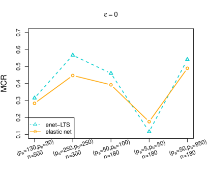
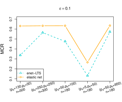
Figure 1: Misclassification rate (MCR) for the different settings. Left: clean data; right: 10% contamination in informative variables only.

The precision of the informative variables in Fig. 2 decreases with the decreasing rate of $p_{a}/p_{b}$, thus with increasing model sparsity. This decrease is also connected to a decrease of FPR (Fig. 4 left) and an increase in FNR (Fig. 5 left), for increasing sparsity. This means that for less sparse models, the methods tend to include noise variables, while for sparser models, they tend to exclude informative variables. Thus, the block of non-zero regression coefficients might be easier to being recovered if sparsity increases, and if estimated zeros appear in this block.

The precisions for the informative variables are slightly better for the classical elastic net estimator in the uncontaminated case, and slightly better for enet-LTS with contaminated data (Fig. 2). The precision of the uninformative variables in Fig. 3 is quite comparable for the two estimators in the uncontaminated case, except for setting 4. Interestingly, enet-LTS is a bit better for the uncontaminated data, but elastic net has better performance in the contaminated case. However, when comparing the scale for the precision of the informative and uninformative variables, we see that these differences in the uninformative case are quite marginal.

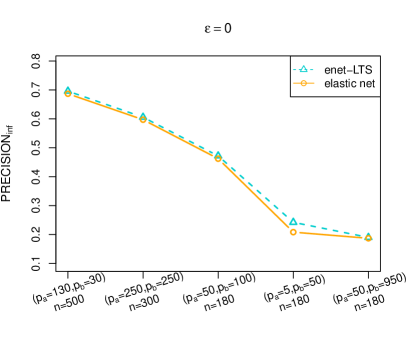
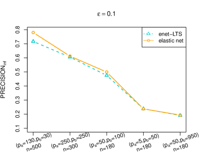
Figure 2: Precision of the estimated coefficients for informative variables ($\mathrm{PRECISION_{inf}}$) for the different settings. Left: clean data; right: 10% contamination in informative variables only.

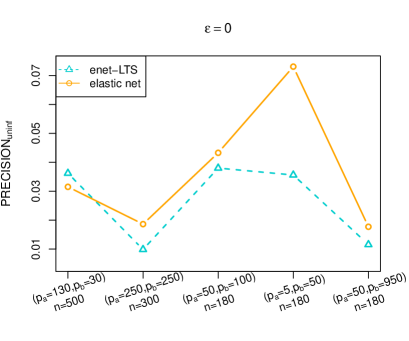
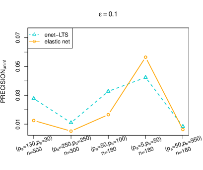
Figure 3: Precision of the estimated coefficients for uninformative variables ($\mathrm{PRECISION_{uninf}}$) for the different settings. Left: clean data; right: 10% contamination in informative variables only.

Fig. 4 and Fig. 5 show the quality of the variable selection ability of the estimators with respect to FPR and FNR. Both measures complement each other: when FPR increases, FNR decreases, and vice versa. The picture for enet-LTS is quite comparable in the uncontaminated and contaminated case, while for the classical estimator we see a completely different behavior: In case of contamination, the FNR increases enormously in almost all settings, thus far too few informative variables are selected. Compared to the uncontaminated case, the FPR can be reduced, which means a reduction of incorrectly selected noise variables. In other words, the classical estimator tends to produce much higher sparsity in presence of contamination.

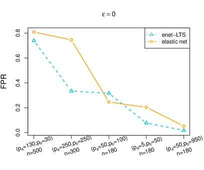
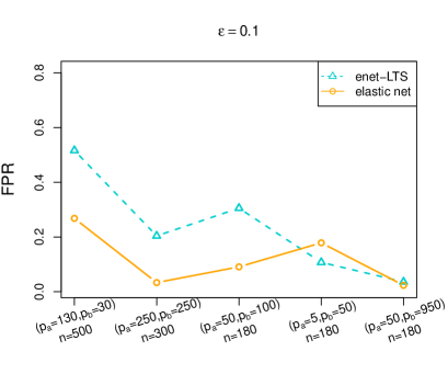
Figure 4: False positive rate (FPR) for the different scenarios. Left: clean data; right: 10% contamination in informative variables only.

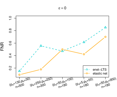
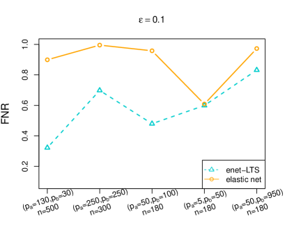
Figure 5: False negative rate (FNR) for the different scenarios. Left: clean data; right: 10% contamination in informative variables only.

5 Real data applications

5.1 Analysis of handwritten digits

We consider a data set with normalized handwritten digits, which is available from the R package [18] and goes back to [12]. This quite famous data set has been used a lot in machine learning, and it consists of images with scanned digits from envelopes of delivered letters from the the U.S. Postal Service. The images with the digits 0 to 9 (thus there are 10 groups) have been preprocessed to 16 $\times$ 16 grayscale images. We fit our model to the training set consisting of 7291 observations, and evaluate for the test set which has 2007 observations. Table 2 shows the resulting confusion table for the training data, and Table 3 that for the test data. The correct classification rate is 88.1% for the training data, and 84.3% for the test data. One can see that the misclassifications are quite different among the different digits, depending on whether these are very similar or not. For example, digit “4” is frequently misclassified as digit “1”, “2”, or “9”. Compared to other classifiers, especially from machine learning, see http://yann.lecun.com/exdb/mnist/, our results for the correct classification rate are not too exciting, but we can get interesting interpretations, as seen in the following.

		Predicted class
		0	1	2	3	4	5	6	7	8	9
True class	0	1067	0	20	7	15	10	41	6	23	5
	1	0	996	0	0	0	0	0	0	8	1
	2	13	1	640	13	14	0	3	14	27	6
	3	1	1	14	576	2	22	0	10	24	8
	4	1	34	25	0	551	1	11	0	9	20
	5	12	1	10	25	31	456	4	5	8	4
	6	10	4	39	0	13	16	568	0	14	0
	7	1	2	17	0	34	10	0	529	4	48
	8	7	3	10	19	14	11	3	3	465	7
	9	4	2	2	1	12	17	0	23	8	575

Table 2: Confusion table for the training data of the handwritten digits data set.

		Predicted class
		0	1	2	3	4	5	6	7	8	9
True class	0	317	0	11	3	4	1	15	0	4	4
	1	0	251	1	2	4	0	2	0	2	2
	2	6	0	157	6	9	1	1	2	16	0
	3	5	0	4	128	3	14	0	1	6	5
	4	1	9	7	0	164	0	3	1	4	11
	5	8	0	0	10	9	123	0	0	4	6
	6	5	0	10	0	3	7	142	0	3	0
	7	1	2	4	0	15	0	0	118	1	6
	8	4	0	1	12	5	4	2	1	132	5
	9	0	2	0	1	4	2	0	7	2	159

Table 3: Confusion table for the test data of the handwritten digits data set.

In order to understand how the classifier works and which pixel information is important for the class assignments, we show a plot of the regression coefficient matrix in Figure 6. Every plot is for one digit (legend on top), and consists of 16 $\times$ 16 regression coefficients presented as image. Darker color means higher coefficient, red for positive, blue for negative. White refers to zero coefficients. Some of the coefficients are quite sparse, such as those for digit “1”, others have almost no zeros. Since the input data are scaled in $[-1,1]$, and higher values refer to darker image information, we can say that positive coefficients increase the probability of assignment to a class. Accordingly, Figure 6 shows well with red color which pixels are important for the class assignment, and which contribute negatively (blue). There seem to be some specifics related to the style how the digits are written, seen for example in the upper right part of digit “5”.

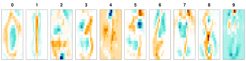
Figure 6: Visualization of the estimated regression coefficients.

This “typical” shape of the handwritten digits mentioned above can be extracted from our results. According to Equation (8) we can compute for every observation of the training data a robust Mahalanobis distance. Figure 7 shows the images with the smallest distances per class, and thus these would correspond to the most “inlying” and thus typical writing styles of the digits. On the other hand, Figure 8 shows the most outlying training set observations per class, which are those observations of each class with the biggest distance.

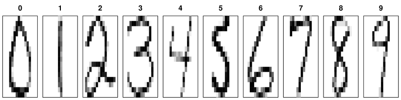
Figure 7: Most “inlying” digits according to the model.

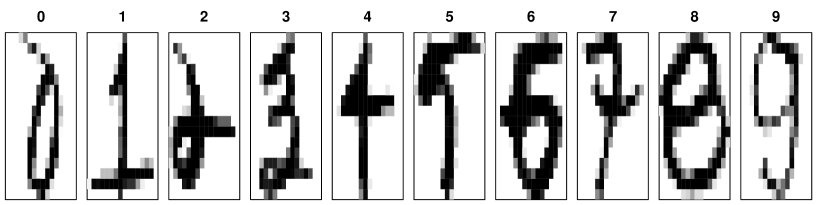
Figure 8: Most outlying digits of each group.

Figure 9 shows the ten observations from the test set which should represent digits “5”, but are incorrectly classified as digit “3”, see also Table 3. Looking at the coefficients in Figure 6, the lower part in the image is very similar, but the upper part should indicate the major differences; in particular, digit “5” is expected to have dark pixel information in the upper right corner, which is not the case for digit “3”. Indeed, this is what most of the images in Figure 9 are missing. Other digits show different major differences to an expected “5” also mainly in the upper part.

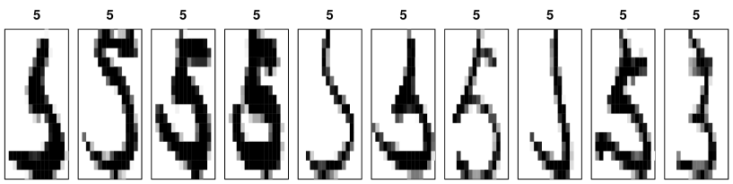
Figure 9: Digits “5” from the test set, wrongly classified as “3”.

5.2 Analysis of the fruit data set

This data set has been used previously in the context of robust discrimination, for example in [8]. It contains spectral information with 256 wavelengths, thus is high-dimensional, for observations from 3 different cultivars of the same fruit, named D, M, and HA, with group sizes 490, 106, and 499. Group D in fact consists of two sub-groups, because for 140 observations a new lamp has been installed in the measurement device. As we have no information about the membership of these subgroups, we treat them as one group. Also group HA should consist of 3 sub-groups due to a change of the illumination system, and also this group was treated as a single group.

Applying our estimator yields the estimated coefficients visualized in Figure 10, which shows the 256 values per group as lines. One can see that the model yields a very sparse solution. The first wavelength range which looks rather confusing seems to be important for the classification task.

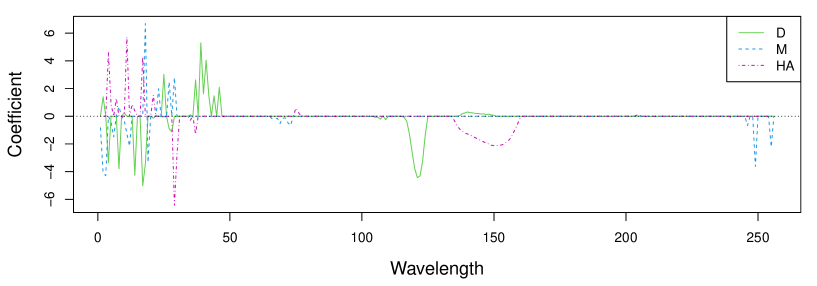
Figure 10: Estimated coefficients for the fruit data set.

The model has a correct classification rate of about 87%, well balanced over the groups. However, we did not go into a deeper evaluation of the classification performance by using cross-validation. Five-fold cross-validation has been used inside the procedure for selecting the optimal tuning parameters. Here we have forced $\alpha$ to be higher, yielding more sparsity. With the optimal value of $\alpha$ we would have had no sparsity at all, but an improved error rate of about 95%.

We computed the scores matrix $\mathbf{Z}_{l}$, for $l=1,2,3$, see Section 2.2, and the resulting scaled robust distances, see Equation (8). Figure 11 (left) shows the scores of all groups in the space of the first two principal components, explaining nearly all of the variability. The symbol colors are according to the group memberships, and the symbols according to the scaled distance: a rhombus if this distance was 1, and a “+” otherwise. For group HA we can indeed see that a big part of the observations has been identified as outliers, or at least as unusual observations. Also for group D we can see several outliers. The right plot of this figure shows a ternary plot with the estimated probabilities, again using the same symbols as before. Most observations are close to the edge of the triangle, and thus they are correctly assigned to the corresponding class. Many of the outliers from the HA group are wrongly assigned to group M or D, which also reduces the correct classification rate. If one would exclude the observations with scaled distance smaller than one from the error rate calculation, the correct classification rate would be higher than 99%.

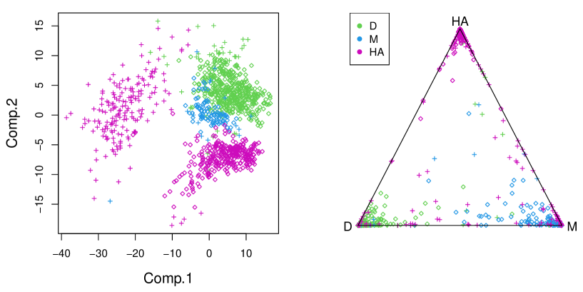
Figure 11: First two principal components of the estimated scores (left) and classification probabilities (right) for the fruit data set.

6 Conclusions

This paper introduced a robust and sparse method for multinomial regression. The method is able to identify outliers in high-dimensional data, as well as mislabeled observations, thus observations which rather belong to a different group, and it downweights such outliers in the estimation procedure. In contrast to linear discriminant analysis, the multinomial regression model directly specifies the parameters which relate the variables to the classification problem, and this supports the interpretability of the estimated parameters. In a sparse setting, non-zero parameters will be connected to informative variables, while uninformative noise variables are associated with zero parameters. In presence of outliers, a robust method is supposed to not only return reliable parameter estimates, but also a reliable identification of relevant and noise variables.

The idea to achieve robustness for the parameter estimation is based on trimming the penalized negative log-likelihood function [5], similar as it has been proposed for robust logistic regression in high dimensions [10]. Outliers are identified in the space of the scores, which are the values of the linear link function. The score space has at most dimension $K-1$, where $K$ is the number of groups, and thus group-wise robustly estimated (and scaled) Mahalanobis distances can be used for the purpose of outlier identification. The score space is also very useful for visual data exploration and interpretation. Finally, the outlyingness information can be incorporated in weights to obtain a reweighted estimator which achieves higher efficiency than the trimmed estimator. Sparsity is obtained by using an elastic net penalty, which results in an intrinsic variable selection property besides dealing with the multicollinearity problem, and therefore the proposed method is very useful in high-dimensional sparse settings.

We have conducted simulations to compare the proposed estimator with its non-robust counterpart introduced in [5]. Hereby, various scenarios such as $n>p$, $p>n$, and increasing sparsity levels have been considered. For uncontaminated data, the robust estimator sometimes tends to lead to a higher false negative rate than the classical estimator, and thus to a sparser model. In contrast, the false positive rate is often smaller than for the classical estimator, which means to obtain fewer false discoveries. Again, depending on the setting, the robust estimator can lead to a (slightly) increased misclassification error. In presence of contamination we have seen that the robust estimator leads to a performance which is very similar to the uncontaminated case, while the classical estimator is severely influenced by the outliers.

Finally, the real data applications in Sec. 5 revealed the usefulness of the proposed estimator. Plots of the estimated regression parameters lead to very interesting conclusions, since we can see which variables (pixels, wavelengths) are important for the classification task. Also the outlyingness information and the visualization of the scores is highly useful for a deeper understanding of the problem.

The algorithm for computing the estimator has been implemented in the R package enetLTS [11]. This package is using internally the R package glmnet [6] which also implements Poisson, Cox and multivariate regression. As a matter of course, in our future work we plan to extend the introduced algorithm to these models.

References

- [1] Akdeniz, F. and Erol, H. 2003. Mean Squared Error Matrix Comparisons of Some Biased Estimators in Linear Regression. Communications in Statistics: Theory and Method, 32 (12):2389-2413.
- [2] Daniel, C. and Wood, F. S. 1980. Fitting equations to data: computer analysis of multifactor data. 2nd edn. In: With the assistance of John W. Gorman. Wiley, New York.
- [3] Farebrother, R.W. 1976. Further Results on the Mean Square Error of Ridge Regression. Journal of the Royal Statistical Society Series B, 38(3):248-250.
- [4] Hald, A. 1952. Statistical Theory with Engineering Applications., New York: Wiley.
- [5] Hoerl, A.E. and Kennard, R.W. 1970. Ridge Regresssion: Biased Estimation for Nonorthogonal Problems. Technometrics, 12(1):55-67.
- [6] Hoerl, A.E., Kennard, R.W., and Baldwin, K. F., 1975. Ridge Regression: Some Simulation, Communications in Statistics: Theory and Methods, 4:105-123.
- [7] Liu, K. 1993. A New Class of Biased Estimate in Linear Regression Communications in Statistics: Theory and Methods, 22(2):393-402.
- [8] Liu, K. 2003. Using Liu-Type Estimator to Combat Collinearity. Communications in Statistics: Theory and Methods, 32(5):1009-1020.
- [9] Kibria,B.M.G. 2003. Performance of some new ridge regression estimators, Communications in Statistics - Simulation and Computation, 32(2):419-435.
- [10] Kurnaz, F.S., Akay, K.U. 2015. A new Liu-type estimator, Statistical Papers, 56:495-517.
- [11] Lawless, J.F., Wang, P., 1976. A Simulation Study of Ridge and Other Regression Estimators, Communications in Statistics: Theory and Methods, 5 (4):307-323.
- [12] McDonald, G.C., Galarneau, D.I. 1975. A monte carlo evaluation of some ridge-type estimators, Journal of American Statistical Assossiation, 70:407-416.
- [13] Sakallioglu, S., Kaciranlar, S. 2008. A New Biased Estimator Based on Ridge Estimation, Statistical Papers, 49:669-689.
- [14] Sakallioglu, S., Kaciranlar, S., Akdeniz F. 2001. Mean Squared Error Comparisons of Some Biased Regression Estimators, Communications in Statistics: Theory and Methods, 30(2):347-361.
- [15] Stein, C. 1956. Inadmissibility of the usual estimator for the mean of a multivariate normal distribution, in: Proceedings of the Third Berkeley Symposium on Mathematics, Statistics and Probability, University of California Press, Berkeley.
- [16] Theobald, C. M. 1974. Generalizations of mean square error applied to ridge regression. Journal of the Royal Statistics Society Series B, 36(1):103-106.
- [17] Trenkler, G., Toutenburg, H. 1990. Mean Squared Error Matrix Comparisons between Biased Estimator-An Overview of Recent Results, Statistical Papers, 31:165-179.
- [18] Yang, H., Chang, X., 2010. A New Two-Parameter Estimator in Linear Regression, Communications in Statistics: Theory and Methods, 39(6):923-934.
- [19] Woods, H., Stenior, H. H., Starke, H. R. 1932. Effect of composition of Portland cement on heat evolved during hardening. Industrial and Eng Chem, 24:1207-1214.
- [20] R Development Core Team, R: A Language and Environment for Statistical Computing, Vienna, Austria, R Foundation for Statistical Computing, Vienna, Austria, (2021). URL http://www.R-project.org