Hedging Valuation Adjustment and Model Risk

Abstract

The dynamic hedging theory only makes sense in the setup of one given model, whereas the practice of dynamic hedging is just the opposite, with models fleeing after the data through daily recalibration. In this paper we revisit Burnett (2021) & Burnett and Williams (2021)’s notion of hedging valuation adjustment (HVA), originally intended to deal with dynamic hedging frictions, in the direction of model risk. We formalize and quantify Darwinian model risk as introduced in Albanese, Crépey, and Iabichino (2021), in which traders select models producing short to medium term gains at the cost of large but distant losses. The corresponding HVA can be seen as the bridge between a global fair valuation model and the local models used by the different desks of the bank. Importantly, model risk and dynamic hedging frictions indeed deserve a reserve, but a risk-adjusted one, so not only an HVA, but also a contribution to the KVA of the bank. The orders of magnitude of the effects involved suggest that bad models should not so much be managed via reserves, as excluded altogether. Model risk on CVA and FVA metrics is also considered.

Keywords: pricing models, model risk, calibration, market risk, counterparty credit risk, transaction costs, cross valuation adjustments (XVAs).

Mathematics Subject Classification: 91B25, 91B26, 91B30, 91G20, 91G40.

JEL Classification: D52, G13, G24, G28, G32, G33.

1 Introduction

The 2008 global financial crisis triggered a shift from trade-specific pricing to netting-set CVA analytics. For tractability reasons, the market models used by banks for their CVA analytics are simpler than the ones that they use for individual deals. Given this coexistence of models, it is no surprise if FRTB emphasized the issue of model risk.

In the context of structured products, Albanese, Crépey, and Iabichino (2021) introduced the notion of Darwinian model risk, whereby the trader of a bank prefers to a reference fair valuation model an alternative pricing model, which renders a trade more competitive (more attractive for clients) in valuation terms. The trader thus closes the deal at some valuation loss, but the latter is more than compensated by gains on the hedging side of the position. However these overall positive gains on the product and its hedge are only a short to medium term view. In the long run, large losses are incurred by the bank when market conditions reveal the unsoundness of the trader’s pricing and hedging model.

Under current market practice endorsed for instance in European Parliament (2016, L 21/54, point (2)), model risk is accounted for by setting aside as a reserve the difference between (buying) prices in bad models and prices in good models. While this indeed corresponds to the first layer of defence against model risk as derived in this paper, we further argue that this is not enough, as long as hedges are still computed using the bad models. We propose to revise model risk reserves by adding an add-on sensitive to hedge ratios. Toward this aim, we encompass the Darwinian model risk of Albanese, Crépey, and Iabichino (2021) in a cost-of-capital XVA framework, proposing a reserve for model risk and dynamic hedging frictions in two parts: an HVA component, encapsulating Burnett (2021) & Burnett and Williams (2021) within a broader model risk perspective; this HVA can be seen as the bridge between a global fair valuation model and the local models used by the different desks of the bank, restoring the correct prices that should have been used by traders in the first place. Then the reserve is risk-adjusted, via a KVA component accounting for the erroneous hedges.

1.1 Related Literature

We refer to Detering and Packham (2016) and the references therein, in particular (Karoui, Jeanblanc-picqué, and Shreve, 1998; Cont, 2006; Elices and Giménez, 2013), for a discussion about model risk and the associated regulatory guidelines until 2014. Other related references include Barrieu and Scandolo (2015), who “introduce three quantitative measures of model risk when choosing a particular reference model within a given class”, or Farkas, Fringuellotti, and Tunaru (2020), who “propose a general method to account for model risk in capital requirements calculus related to market risk”. Model uncertainty is considered at the level of individual deals by Bartl, Drapeau, Obloj, and Wiesel (2021), who consider uncertainty in a Wasserstein ball around a reference probability measure. While the ensuing price is robust, the associated hedge is necessarily imperfect, and capital implications are not considered. To address the model risk and uncertainty quantification issues, in the context of financial derivatives, we prefer to worst-case approaches the HVA take of this paper, risk-adjusted and eventually made Bayesian-robust the way explained in Remark 6.1. We think that this is more scalable and does better justice to considerations of model realism than robust approaches that are typically over-conservative, hence unusable in practice for competitiveness reasons, let aside major computational issues at large scale.

The model risk specific to XVA computations is also considered in the literature. Bichuch, Capponi, and Sturm (2020) and Silotto, Scaringi, and Bianchetti (2021) consider parameters uncertainty. Singh and Zhang (2019b, a) consider uncertainty around a reference probability measure in the Wasserstein distance, in a discrete time setting and for a finitely supported reference measure. Regarding our baseline cost-of-capital XVA approach, Bichuch, Capponi, and Sturm (2020) write in their introduction: “Despite the merits of this approach, in particular not having to rely on replication arguments for the value adjustments, it makes two critical assumptions. First, it assumes that the counterparty-free payoffs of the contract are perfectly replicated, rather than designing the replication strategy from first principles (and ignoring potential interaction of risk factors). Second, and most importantly, they assume that the historical and risk-neutral probability measure coincide. This, of course, exposes the calculation of the valuation adjustments to a substantial amount of model risk, which can be accounted for by the techniques proposed in this paper.” The present paper provides an answer to their first point, by reintroducing unhedged market risk (via Darwinian model risk) into the XVA computations (as for their second point, we do not assume that the historical and risk-neutral probability measure coincide, cf. Definition 1.1).

1.2 Outline of the Paper and Standing Notation

Section 2 introduces Darwinian model risk at the level of individual deals. Section 3 casts the ensuing hedging valuation adjustment (HVA). Overhauling Burnett (2021) in a setup also accounting for model risk, Section 4 deals with the HVA for dynamic hedging frictions at the hedging set level. Section 5 addresses the related contributions to the KVA of the bank. So far this was all restricted to market risk. Section 6 retrieves the CVA and FVA components of the HVA, thus incorporating the HVA into the global valuation framework of Albanese et al. (2021) & Crépey (2022), and concludes.

All processes are adapted to the filtration $\mathfrak{F}=(\mathfrak{F}_{t})$ of a reference stochastic basis. The risk-free asset is chosen as numéraire. We denote by $\overline{T}$, a bound on the final maturity of the bank portfolio; $\bm{\delta}_{\vartheta}$, a Dirac measure at a stopping time $\vartheta$; $X^{\vartheta}$, a process $X$ stopped at time $\vartheta$; $X_{(0)}=X-X_{0}$, for any process $X$; $\mathcal{N}$, the standard normal cumulative distribution function. When no ambiguity arises we denote the time process by $t$, as in $N-\lambda t$ to denote a compensated Poisson process of intensity $\lambda$.

Fair Valuation

In the incomplete market setup intrinsic to the XVA issue (Albanese et al., 2021, Section 3.5), our reference probability measure $\mathbb{R}$ is the hybrid of pricing and physical probability measures advocated in Albanese et al. (2021, Remark 2.3), with related time-$t$ expectation, value-at-risk, and expected shortfall denoted by $\mathbb{E}_{t}$, $\mathbb{V}a\mathbb{R}_{t}$ and $\mathbb{ES}_{t}$ (and for $t=0$, we drop all indices $t$):

Definition 1.1.

Let there be given a $\sigma$-field $\mathcal{A}$, on which the physical probability measure $\mathbb{P}$ is defined, and a financial sub-$\sigma$-field $\mathcal{B}$ of $\mathcal{A}$, on which a risk-neutral measure $\mathbb{Q}$, equivalent to the restriction to $\mathcal{B}$ of the physical probability measure, is defined. Our probability measure $\mathbb{R}$ in the paper is the uniquely defined probability measure on $\mathcal{A}$, provided by Artzner, Eisele, and Schmidt (2022, Proposition 4.1.), such that (i) $\mathbb{R}$ coincides with $\mathbb{Q}$ on $\mathcal{B}$ and (ii) $\mathbb{R}$ and $\mathbb{P}$ coincide conditionally on $\mathcal{B}.\$

Remark 1.1.

Until Section 6, the bank and its clients are assumed to be default-free. The realistic extension to defaultable entities is provided in Section 6.1. The probability measure with respect to which $\mathbb{E}_{t}$, $\mathbb{V}a\mathbb{R}_{t}$ and $\mathbb{ES}_{t}$ are defined then becomes the bank survival probability measure associated with $\mathbb{R}$ in the sense of Albanese et al. (2021, Section 4); see also Crépey (2022, Section B) for a practically equivalent reduction of filtration viewpoint.

All (cumulative) cash flows are finite variation processes (starting from 0) and all prices are special semimartingales in a càdlàg version. We use the calligraphic style (e.g. $\mathcal{Y}$) for cash flows and the italic style (e.g. $Y$) for prices, in uppercase versus lowercase styles to distinguish between fair versus trader valuations, e.g. $Q$ versus $q$.

Definition 1.2.

Given an optional, integrable process $\mathcal{Y}$ stopped at $\overline{T}$, its value process $Y=va(\mathcal{Y})$ is

$$Y_{t}=\mathbb{E}_{t}({\mathcal{Y}}_{{\overline{T}}}-{\mathcal{Y}}_{t}),\,t\leq{\overline{T}},$$ (1.1)

and $Y$ vanishes on $[{\overline{T}},+\infty).\$

In particular, $(\mathcal{Y}+Y)$ is a martingale on $[0,\overline{T}]$. Fair valuation comes in contrast with the local models that are effectively used by the traders of the bank. The existence and availability of a fair valuation setup is an idealization and simplification, but it is a legitimate and useful one in the context of model risk, which as we shall see is a lot about alpha leakages, i.e. drifts that only cumulate into sizeable effects over months or years. The usual risk metrics, whether it is value-at-risk, expected shortfall or stressed value-at-risk, do not detect alpha leakages because they focus on higher moments of return distributions and on short-time horizons (such as one day). As already experienced in the quantitative reverse stress test setup of Albanese, Crépey, and Iabichino (2023), the only way to detect Darwinian model risk is by simulating the hedging behavior of a bad model within a good model.

2 Darwinian Model Risk

In this section we describe our model risk setup, dubbed Darwinian model risk, for each deal of the bank with a client.

2.1 Client Deals Cash Flows

Notation 2.1.

In reference to a generic deal “$\cdot$” of the bank with a client, we define:

• $T^{\cdot}$, the maturity of the deal;

• $\mathcal{Q}^{\cdot}$, the cumulative cash flow process contractually promised by the counterparty to the bank;

• $0<\tau_{e}^{\cdot}\leq T^{\cdot}$, a deactivation time (possibly $<T^{\cdot}$ for products with knock-out features).

Remark 2.1.

We could also consider American or game claims with exercise times possibly $<T^{\cdot}$ under the control of the bank and/or client, in which case $\tau_{e}^{\cdot}$ should be understood as the corresponding exercise time. Callability by the bank is actually the source of Darwinian model risk in Albanese, Crépey, and Iabichino (2021). Further adjustments are then required to deal with possibly suboptimal stopping by the bank (suboptimal stopping by the client can be conservatively ignored in the modeling). These adjustments are the topic of Benezet, Crépey, and Essaket (2022). In the present paper we assume no American early exercise features.

In the defaultable extension of the theory provided by Section 6.1, $\tau_{e}^{\cdot}$ should be replaced everywhere by $\tau_{d}^{\cdot}\wedge\tau_{e}^{\cdot}$, where $\tau_{d}^{\cdot}$ denotes a positive default time of the counterparty of the deal (the default of the bank itself is absorbed in the switch to its survival measure mentioned in Remark 1.1).

The following example will be continued throughout the article in order to help understand the abstract setting and quantify various effects numerically.

Example 2.2.

We consider a financial derivative on a stock $S$, dubbed vulnerable put, whereby the bank is long the payoff $(K-S_{T})^{+}\mathds{1}_{\{{S_{T}>0}\}}$ at some maturity $T$, for some strike $K$ (with $T,K,S\geq 0$). In Notation 2.1, we have here

$$T^{\cdot}=T,\mathcal{Q}^{\cdot}_{t}=(K-S_{T})^{+}\mathds{1}_{\{{S_{T}>0}\}}\mathds{1}_{[T,+\infty)},\,\tau_{e}^{\cdot}=T.\$$

2.2 Client Deals Valuation

Instead of fair valuation, we assume that the trader in charge of the deal “$\cdot$” within the bank uses, at least up to some stopping time, a custom or “local” model. More precisely:

Assumption 2.2.

1. For pricing, hedging and accounting purposes, before a positive stopping time $\tau_{s}^{\cdot}$ coined model switch time, the trader of the deal makes use of a local pricing model, giving rise to a price process $q^{\cdot}$ for the deal;

2. If $\tau_{s}^{\cdot}<T^{\cdot}$, from time $\tau_{s}^{\cdot}$ onwards, the bank uses the fair valuation $Q^{\cdot}=va(\mathcal{Q}^{\cdot})$ of the deal for pricing, hedging and accounting purposes.

Here “local” stands in contrast with the assumed global fair valuation setup, see after Definition 1.2. Note that Assumption 2.2 is in line with the qualitative features of Darwinian model risk introduced in Section 1. The chief goal of this work is to quantify the latter in a suitable XVA framework.

Example 2.3.

In our vulnerable put Example 2.2, with dividend yields on $S$ and interest rates in the economy set to 0, the role of the fair valuation model will be played by the jump-to-ruin ($jr$) model

$$\begin{aligned} dS_{t}=\lambda S_{t}dt+\sigma S_{t}dW_{t}-S_{t-}dN_{t}=\sigma S_{t}dW_{t}-S_{t-}dM_{t},\quad t\geq 0,\end{aligned}$$ (2.1)

for some standard Brownian motion $W$, a constant volatility parameter $\sigma>0$, and $M=N-\lambda t$, where $N$ is a Poisson process of intensity $\lambda>0$. So the stock $S$ jumps to 0 at the first jump time $\theta$ of the driving Poisson process $N$. Hence, denoting by $J^{\theta}_{t}=\mathds{1}_{\{{t<\theta}\}}$ the indicator process of $\theta$,

$$\begin{aligned} Q^{\cdot}_{t}&=va(\mathcal{Q}^{\cdot})_{t}=Q^{jr}_{t}:=\mathbb{E}_{t}\left[(K-S_{T})^{+}J^{\theta}_{T}\right]\mathds{1}_{\{{t<T}\}},\,t\geq 0.\end{aligned}$$ (2.2)

The role of the local pricing model will be played by a Black-Scholes (bs) model with volatility parameter $\Sigma$ continuously recalibrated to the jump-to-ruin price

$$\begin{aligned} P^{jr}_{t}:=\mathbb{E}_{t}\left[(K-S_{T})^{+}\right]\mathds{1}_{\{{t<T}\}},\,t\geq 0\end{aligned}$$ (2.3)

of the “vanilla component” of the vulnerable put, with payoff $(K-S_{T})^{+}$ at time $T$. We also define $\tau_{s}^{\cdot}:=\theta$ and $q^{\cdot}_{t}=P^{jr}_{t}.$ Indeed, an application of the formula (A.13) for $S=0$ and $-d_{\pm}=+\infty$ shows that $P^{jr}=K$ on $\llbracket\theta,\theta\wedge T\llbracket$. As detailed in Remark A.1, at time $\theta$ (if $<T$), the implied volatility of the vanilla put ceases to be well-defined, hence the local pricing model cannot be used anymore. Before $\theta$, in accordance with Assumption 2.2, the trader uses his local pricing model. But the vulnerability of the put is immaterial in this model, hence the bs price of the vulnerable put coincides with the vanilla put price $P^{jr}_{t}.\$

Remark 2.4.

So, in our example, the trader is short an extreme (default) event but pretends he does not see it, only hedging market risk. Hence the hedged position is still short the default event, which can be seen as an extreme case of “gamma negative” type position. This example is devised for the sake of analytical tractability. Yet the Darwinian model risk mechanism at hand here is essentially the same as the one affecting huge amounts of structured derivative products, including range accruals in the fixed-income world, autocallables and cliquets on equities, or power-reversal dual currency options and target redemption forwards on foreign-exchange: cf. https://www.risk.net/derivatives/6556166/remembering-the-range-accrual-bloodbath (11 April 2019, last accessed on 30 November 2023). Risk.net thus reported that Q4 of 2019, a $70bn notional of range accrual had to be unwound at very large losses by the industry.

2.3 Client Deals Hedges

Each deal “$\cdot$” can be hedged statically and/or dynamically. Accordingly (cf. Notation 2.1):

Notation 2.3.

Given the client deal “$\cdot$”, we define:

• $\mathcal{P}^{\cdot}$, the cumulative cash flow process paid by the bank on a static hedge component of the deal;

• $P^{\cdot}=va(\mathcal{P}^{\cdot}),$ the fair valuation of this static hedge;

• $p^{\cdot},$ the price process of the static hedge in the local pricing model of the deal (before time $\tau_{s}^{\cdot}$);

• $h^{\cdot},$ a dynamic hedging loss of the bank related to the deal, ignoring transaction costs.

In particular, a natural assumption regarding $h^{\cdot}$ is:

Assumption 2.4.

$h^{\cdot}$ is a zero-valued martingale stopped at $\tau_{e}^{\cdot}$, i.e. $h^{\cdot}=(h^{\cdot})^{\tau_{e}^{\cdot}}$ and $va(h^{\cdot})=0.\$

Remark 2.5.

We do not assume a frictionless market. But numerous deals are hedged together inside “hedging sets” by the bank. Hence market frictions such as transaction costs can only be addressed at the hedging set level, which will be the topic of Section 4.

The fair valuation prices $Q^{\cdot}$ and $P^{\cdot}$, being value processes of cash flow processes stopped at maturity $T^{\cdot}$, vanish on $[T^{\cdot},+\infty)$. Likewise:

Assumption 2.5.

The processes $q^{\cdot}$ and $p^{\cdot}$ vanish on $[T^{\cdot},+\infty).\$

We now introduce two reference hedging schemes for the vulnerable put of Example 2.2.

Example 2.6 (Static hedging).

The trader uses at time $t=0$ the local (bs) pricing model, in which the vulnerability of the put is immaterial. From the bs model viewpoint, shorting the vanilla put is a perfect hedge to the vulnerable put and no dynamic hedging is required. In Notation 2.3, this corresponds to $h^{\cdot}=0$ and

$$\begin{aligned} &\mathcal{P}^{\cdot}=(K-S_{T})^{+}\mathds{1}_{[T,+\infty)},\\ &p^{\cdot}=P^{\cdot}=va(\mathcal{P}^{\cdot})=P^{\textit{jr}}\mbox{ as per \eqref{Pjr}}.\end{aligned}$$ (2.4)

The definition of $p^{\cdot}$ means that the local pricing model is continuously recalibrated (before the ruin time $\theta$) to the vanilla put fair valuation $P^{jr}$, the way explained in Example 2.3.

Example 2.7 (Delta hedging).

The trader delta hedges the vulnerable put with the stock $S$ and the risk-free asset, in his local bs pricing model and until time $\theta$, and there is no static hedging. In Notation 2.3, we have

$$\begin{aligned} &\mathcal{P}^{\cdot}=P^{\cdot}=p^{\cdot}=0\mbox{ and }h^{\cdot}_{t}=\int_{0}^{t}\delta_{s}dS_{s},\end{aligned}$$ (2.5)

where $\delta_{t}=\delta_{t}J^{\theta}_{t}$ is the delta of the vulnerable put computed in the local pricing model (if $t<\theta$, i.e. as long as the latter can be calibrated). Note that, in this setting, dynamic hedging friction costs can be considered, namely transaction costs, which will be done in Section 4.4.

3 HVA for Individual Deals

In this section we consider the hedging valuation adjustment (HVA) triggered by each individual deal “$\cdot$” of the bank.

Under Assumptions 2.2-2.4, the deal and its hedge are liquidated at time $\tau_{e}^{\cdot}$ and there is a model switch at $\tau_{s}^{\cdot}$. Accordingly, using Notations 2.1 and 2.3 and setting $J^{s,\cdot}_{t}=\mathds{1}_{\{{t<\tau_{s}^{\cdot}}\}}$:

Definition 3.1.

The raw pnl of the client originating deal derivative “$\cdot$” of the bank is the process

$$pnl^{\cdot}=\big{(}\mathcal{Q}^{\cdot}+J^{s,\cdot}q^{\cdot}+(1-J^{s,\cdot})Q^{\cdot}\big{)}^{\tau_{e}^{\cdot}}_{(0)}-\big{(}\mathcal{P}^{\cdot}+J^{s,\cdot}p^{\cdot}+(1-J^{s,\cdot})P^{\cdot}\big{)}^{\tau_{e}^{\cdot}}_{(0)}-h^{\cdot}.\$$ (3.1)

This pnl accounts for the switch from local to fair valuation at the model switch time $\tau_{s}^{\cdot}$. It is dubbed raw in the sense that it ignores the to-be-defined ${\rm HVA}^{\cdot}$ liability (as well as the dynamic hedging transaction costs, which can only be assessed at the hedging set level).

Remark 3.1.

The bank may consider liquidating the deal at $\tau_{s}^{\cdot}$ when earlier than $\tau_{e}^{\cdot}$. To render this case, one just needs to replace $\tau_{e}^{\cdot}$ by $\tau_{e}^{\cdot}\wedge\tau_{s}^{\cdot}$ (or $\tau_{d}^{\cdot}\wedge\tau_{e}^{\cdot}$ by $\tau_{d}^{\cdot}\wedge\tau_{e}^{\cdot}\wedge\tau_{s}^{\cdot}$ in the defaultable extension of Section 6.1) everywhere.

We now define the first ${\rm HVA}$ layer, namely one ${\rm HVA}$ per client originating deal and its (assumed frictionless so far) hedge.

Definition 3.2.

For each deal “$\cdot$”, its frictionless ${\rm HVA}$ is

$$\begin{aligned} {\rm HVA}^{\cdot}=-va(pnl^{\cdot}).\ \end{aligned}$$ (3.2)

Lemma 3.1.

We have

$${\rm HVA}^{\cdot}=va(\mathcal{H}^{\cdot}),$$ (3.3)

where

$$\mathcal{H}^{\cdot}:=(\mathcal{Q}^{\cdot}+Q^{\cdot})^{\tau_{e}^{\cdot}}_{(0)}-(\mathcal{P}^{\cdot}+P^{\cdot})^{\tau_{e}^{\cdot}}_{(0)}-pnl^{\cdot}$$ (3.4)

$$\;\;\;\;\;\;\;\;\;=\Big{(}J^{s,\cdot}\big{(}Q^{\cdot}-q^{\cdot}-(P^{\cdot}-p^{\cdot})\big{)}\Big{)}^{\tau_{e}^{\cdot}}_{(0)}+h^{\cdot}.$$ (3.5)

Proof.  (3.1) and (3.4) yield (3.5). Moreover, by the observation following Definition 1.2, $(\mathcal{Q}^{\cdot}+Q^{\cdot})^{\tau_{e}^{\cdot}}_{(0)}$ and $(\mathcal{P}^{\cdot}+P^{\cdot})^{\tau_{e}^{\cdot}}_{(0)}$ are zero-valued martingales. Hence (3.3) proceeds from (3.2).  

Proposition 3.2.

We have

$$\begin{aligned} &{\rm HVA}^{\cdot}=\left(J^{s,\cdot}\big{(}P^{\cdot}-p^{\cdot}-(Q^{\cdot}-q^{\cdot})\big{)}\right)^{\tau_{e}^{\cdot}}-D^{\cdot},\\ &\mathcal{H}^{\cdot}+{\rm HVA}^{\cdot}_{(0)}=h^{\cdot}-D^{\cdot}_{(0)},\end{aligned}$$ (3.6)

where

$$\begin{aligned} D^{\cdot}_{t}=\mathbb{E}_{t}\Big{(}\mathds{1}_{\{{\tau_{e}^{\cdot}<\tau_{s}^{\cdot}\wedge T^{\cdot}}\}}\big{(}P^{\cdot}-p^{\cdot}-(Q^{\cdot}-q^{\cdot})\big{)}_{\tau_{e}^{\cdot}}\Big{)},\,t\geq 0.\end{aligned}$$ (3.7)

In particular,

$${\rm HVA}^{\cdot}_{0}=\big{(}P^{\cdot}-p^{\cdot}-(Q^{\cdot}-q^{\cdot})\big{)}_{0}-\mathbb{E}\Big{(}\mathds{1}_{\{{\tau_{e}^{\cdot}<\tau_{s}^{\cdot}\wedge T^{\cdot}}\}}\big{(}P^{\cdot}-p^{\cdot}-(Q^{\cdot}-q^{\cdot})\big{)}_{\tau_{e}^{\cdot}}\Big{)}.$$ (3.8)

Proof.  By (3.5) and Assumption 2.4, we have for $t\geq 0$:

$$\begin{aligned} &{\rm HVA}_{t}={\mathbb{E}}_{t}\left(J^{s,\cdot}_{\tau_{e}^{\cdot}}\big{(}P^{\cdot}_{\tau_{e}^{\cdot}}-p^{\cdot}_{\tau_{e}^{\cdot}}-(Q^{\cdot}_{\tau_{e}^{\cdot}}-q^{\cdot}_{\tau_{e}^{\cdot}})\big{)}\right)-J^{s,\cdot}_{t\wedge\tau_{e}^{\cdot}}\big{(}P^{\cdot}_{t\wedge\tau_{e}^{\cdot}}-p^{\cdot}_{t\wedge\tau_{e}^{\cdot}}-(Q^{\cdot}_{t\wedge\tau_{e}^{\cdot}}-q^{\cdot}_{t\wedge\tau_{e}^{\cdot}})\big{)},\end{aligned}$$

where $J^{s,\cdot}_{\tau_{e}^{\cdot}}=\mathds{1}_{\{{\tau_{e}^{\cdot}<\tau_{s}^{\cdot}}\}}$ can be replaced by $\mathds{1}_{\{{\tau_{e}^{\cdot}<\tau_{s}^{\cdot}\wedge T^{\cdot}}\}}$ due to Assumption 2.5. This proves the first line in (3.6), which in turn implies that

$$({\rm HVA}^{\cdot}+D^{\cdot})_{(0)}=\left(J^{s,\cdot}\big{(}P^{\cdot}-p^{\cdot}-(Q^{\cdot}-q^{\cdot})\big{)}\right)^{\tau_{e}^{\cdot}}_{(0)}=\mathcal{H}^{\cdot}-h^{\cdot},$$

by (3.5).  

Remark 3.2.

This ${\rm HVA}^{\cdot}$ corresponds to the current market practice for handling model risk, in the form of a reserve put aside at initial time. In actual practice, rather than paying $q_{0}^{\cdot}$ to the client (as implied by (3.1)) while the client would provide ${\rm HVA}^{\cdot}_{0}$ as reserve capital to the bank, the trader pays $Q_{0}^{\cdot}$ to the client and puts by himself ${\rm HVA}^{\cdot}_{0}$ in the reserve capital account, which is equivalent (at least if $D^{\cdot}_{0}=0$ and $P^{\cdot}=p^{\cdot}$, as then ${\rm HVA}^{\cdot}_{0}=q^{\cdot}_{0}-Q^{\cdot}_{0}$).

As will now be illustrated in our vulnerable put example (cf. Remark 2.4), in line with the qualitative features of Darwinian model risk drawn in Section 1, the net ($pnl^{\cdot}-{\rm HVA}^{\cdot}_{(0)}$) martingale (by Definition 1.2) is typically of the “gamma negative” type, i.e. the trader makes systematic profits in the short-to-medium term followed by a large loss at $\tau_{s}^{\cdot}$. This is at least the case unless risk-adjusted model risk provisions, as per Section 5, are used.

3.1 HVA for the Vulnerable Put Under the Static Hedging Scheme

We first consider the static hedging scheme of Example 2.6. Applying (3.1)-(3.6) with $h^{\cdot}=0$ there (as no dynamic hedge is involved), one computes

$$\begin{aligned} &pnl^{\cdot}=-\mathds{1}_{\{\theta\leq T\}}K\mathds{1}_{[T,+\infty)}+(1-J^{\theta})(Q^{\textit{jr}}-P^{\textit{jr}})\\ &\quad=-\mathds{1}_{\{\theta\leq T\}}K\mathds{1}_{[T,+\infty)}-(1-J^{\theta})K\mathds{1}_{[0,T)}\\ &\quad=-\mathds{1}_{\{\theta\leq T\}}K\mathds{1}_{[T,+\infty)}\mathds{1}_{[\theta,+\infty)}-(1-J^{\theta})K\mathds{1}_{[0,T)}\mathds{1}_{\{\theta\leq T\}}=-(1-J^{\theta})K\mathds{1}_{\{\theta\leq T\}}\\ &\mathcal{H}^{\cdot}=J^{\theta}\big{(}Q^{\textit{jr}}-P^{\textit{jr}}\big{)}-\big{(}Q^{\textit{jr}}-P^{\textit{jr}}\big{)}_{0}=-J^{\theta}K(1-e^{-\lambda(T-t)})+K(1-e^{-\lambda T})\\ &{\rm HVA}^{\cdot}=J^{\theta}\big{(}P^{\textit{jr}}-Q^{\textit{jr}}\big{)}=J^{\theta}K(1-e^{-\lambda(T-t)}),\,{\rm HVA}^{\cdot}_{0}=K(1-e^{-\lambda T}).\end{aligned}$$ (3.9)

The raw pnl process in (3.9) and the corresponding pnl net of ${\rm HVA}^{\cdot}_{(0)}$ satisfy (starting at 0)

$$\begin{aligned} &dpnl^{\cdot}_{t}=-K\mathds{1}_{\{{t\leq T}\}}\bm{\delta}_{\theta}(dt)=\mathds{1}_{\{{t\leq\theta\wedge T}\}}\big{(}-\lambda Kdt-(KdN_{t}-\lambda Kdt)\big{)}\\ &dpnl^{\cdot}_{t}-d{\rm HVA}^{\cdot}_{t}=K\mathds{1}_{\{{t\leq\theta\wedge T}\}}e^{-\lambda(T-t)}\big{(}\lambda dt-\bm{\delta}_{\theta}(dt)\big{)}.\end{aligned}$$ (3.10)

Consistently with the qualitative Darwinian model risk pattern featured in Section 1, the seemingly positive drift $\mathds{1}_{\{{t\leq\theta\wedge T}\}}\lambda Ke^{-\lambda(T-t)}dt$ in the second line is only the compensator of the loss $-\mathds{1}_{\{{t\leq\theta\wedge T}\}}Ke^{-\lambda(T-t)}dN_{t}$ that hits the bank in case the jump-to-ruin event materializes.

Numerical Application

For $\lambda=1\%$, $T=10y$ and $K=1$, (3.9) yields

$$\begin{aligned} &{\rm HVA}_{0}=K(1-e^{-0.1})\approx 0.095.\end{aligned}$$ (3.11)

3.2 HVA for the Vulnerable Put Under the Delta Hedging Scheme

We now consider the dynamic delta hedging scheme of Example 2.7. Applying (3.1)-(3.6) with $P^{\cdot}=p^{\cdot}=0$ there (as there is no static hedge involved), we compute with $h^{\cdot}=\int_{0}^{t}\delta_{s}dS_{s}$:

$$\begin{aligned} pnl^{\cdot}&=\mathds{1}_{\{\theta^{\cdot}>T\}}(K-S_{T})^{+}\mathds{1}_{[T,+\infty)}+J^{\theta}P^{\textit{jr}}-P^{\textit{jr}}_{0}-h^{\cdot},\\ \mathcal{H}^{\cdot}&=J^{\theta}(Q^{\textit{jr}}-P^{\textit{jr}})-(Q^{\textit{jr}}-P^{\textit{jr}})_{0}+h^{\cdot}\\ &=-J^{\theta}K(1-e^{-\lambda{(T-t)}}){\mathds{1}_{[0,T)}}+K(1-e^{-\lambda T})+h^{\cdot},\\ {\rm HVA}^{\cdot}&=J^{\theta}(P^{\textit{jr}}-Q^{\textit{jr}})=J^{\theta}K(1-e^{-\lambda(T-t)}),\,{\rm HVA}^{\cdot}_{0}=K(1-e^{-\lambda T}).\end{aligned}$$ (3.12)

The raw $pnl^{\cdot}$ in (3.12), satisfies, for $t<\theta$,

$$\begin{aligned} &dpnl^{\cdot}_{t}=\bm{\delta}_{T}(dt)(K-S_{T})^{+}+dP^{jr}_{t}-\delta_{t}dS_{t},\end{aligned}$$

whereas at $\theta$ (if $\leq T$) the bank incurs a loss

$$\begin{aligned} pnl^{\cdot}_{\theta}-pnl^{\cdot}_{\theta-}&=-P^{jr}_{\theta-}+h^{\cdot}_{\theta-}-h^{\cdot}_{\theta}=-P^{bs}_{\theta-}+\Delta^{bs}_{\theta-}(S_{\theta-}-S_{\theta})\\ &=-P^{bs}_{\theta-}+\Delta^{bs}_{\theta-}S_{\theta-}=-K\mathcal{N}(-d_{-}(\theta,S_{\theta-};0,\Sigma_{\theta-}))<0\end{aligned}$$ (3.13)

(cf. the Black-Scholes formula for puts and (A.2)), consistent again with the blow-up pattern of Darwinian model risk featured in Section 1.

Numerical Application

In the above example, while the static hedge is perfect before $\theta$ and the continuous-time delta hedge is not (due to the continuous recalibration of the local pricing model), one observes a smaller loss at $\theta<T$ in the delta hedging case:

$$\begin{aligned} P^{jr}_{\theta-}-\Delta^{bs}_{\theta-}S_{\theta-}=K\mathcal{N}(-d_{-}(\theta,S_{\theta-};0,\Sigma_{\theta-}))\leq K=P^{bs}_{\theta},\end{aligned}$$

cf. (3.13), (3.10), and the left panel in Figure LABEL:loss-staticdelta.

Remark 3.3.

The statically hedged position is delta and vega neutral. Hence our vulnerable put example yields a case where delta-vega hedging the option actually increases model risk with respect to delta-hedging it.

4 HVA for Dynamic Hedging Frictions

The above processes $h^{\cdot}$ are meant for standard dynamic hedging cash flows ignoring nonlinear frictions such as transaction costs. Indeed, as these are nonlinear, they can only be addressed at the level of each book of contracts or exposures that are hedged together, or hedging sets “$\star$”. In this section we consider the cost of the dynamic hedging frictions assessed at each hedging set level.

Definition 4.1.

Let $f=\sum_{\star}f^{\star}$, the sum of the hedging frictions $f^{\star}$ on each hedging set “$\star$”, and

$$\begin{aligned} {\rm HVA}^{f}=va(f)=\sum_{\star}{\rm HVA}^{\star}\mbox{ , where }{\rm HVA}^{\star}=va(f^{\star}).\ \end{aligned}$$ (4.1)

Remark 4.1.

From an organizational viewpoint, the computation of the ${\rm HVA}^{\cdot}$ components could be delegated to each related trader (under regulatory control). The ${\rm HVA}^{f}$ component(s) calculations would require a dedicated (regulated) HVA desk, as such computations need a mix of data from the different trading desks of the bank.

Hereafter we derive a specification for the cumulative friction costs $f^{\star}$ and for the ensuing ${\rm HVA}^{\star}$, by passage to the continuous-time limit starting from a classical discrete-time specification. This sheds more rigor in the seminal contribution of Burnett (2021), who derives a PDE for the transaction costs at the limit, while only rebalancing when the delta of the underlying portfolio is shifted by a fixed and constant threshold $D>0$ (so it seems that Burnett (2021)’s limiting HVA should rather increase at discrete rebalancing times only, rather than being given by a PDE). Our approach also allows computing ${\rm HVA}^{\star}$ numerically in a model risk setup accounting for the impact of recalibration on transaction costs, which is not considered in Burnett (2021).

4.1 Fair Valuation Setup

In this section we work in the setup of the following fair valuation model stated under the probability measure $\mathbb{R}$, with the risk-free asset as a numéraire:

$$\begin{aligned} &dX_{t}=\mu(t,\mathcal{X}_{t})dt+\sigma(t,\mathcal{X}_{t})dW_{t},\\ &dJ_{t}=\sum_{\jmath=1}^{L}(\jmath-J_{t-})d\nu_{t}^{\jmath},\,\lambda^{\jmath}_{t}=\lambda_{\jmath}(t,\mathcal{X}_{t-}),\end{aligned}$$ (4.2)

where $W$ is a multivariate Brownian motion and $\nu^{\jmath}_{t}$ is the number of transitions of the “Markov chain like” component $J$ to the state $\jmath$ on $(0,t]$, with compensated martingale $d\nu_{t}^{\jmath}-\lambda_{t}^{\jmath}dt$ of $\nu^{\jmath}$. Jumps could also be introduced in $X$ but we refrain from doing so for notational simplicity. This setup encompasses the jr fair valuation model in our vulnerable put example. It also includes XVA models, with space for client default indicator processes in the $J$ components of $\mathcal{X}$, as required in view of our extension of the setup in Section 6.1.

We assume that the function-coefficients $\mu,\sigma,\lambda$ are continuous maps such that the above-model is well-posed, referring to Crépey (2013, Proposition 12.3.7) for a set of explicit assumptions ensuring it. In particular:

Assumption 4.2.

1. The maps $\lambda_{\jmath}$, $1\leq\jmath\leq L$, are bounded by a constant $\Lambda\geq 0$.

2. The map $(t,x,\jmath)\mapsto(\mu,\sigma)(t,x,\jmath)$ is Lipschitz in $x\in\mathbb{R}^{d}$, uniformly in $(t,\jmath)$, and the map $(t,\jmath)\mapsto(\mu,\sigma)(t,0,\jmath)$ is bounded.

Hence (see e.g. Élie (2006, (II.83) page 123)) there exists a constant $C_{1}\geq 0$ such that

$$\begin{aligned} \mathbb{E}\left[\left|X_{t}-X_{s}\right|^{2}\right]^{\frac{1}{2}}\leq C_{1}(t-s)^{\frac{1}{2}}.\end{aligned}$$ (4.3)

In addition, for all $1\leq l\leq d$,

$$\begin{aligned} C^{l}:=\sup_{t\in[0,\overline{T}]}\mathbb{E}\left[(X^{l}_{t})^{2}\right]^{\frac{1}{2}}<+\infty.\ \end{aligned}$$ (4.4)

4.2 Transaction Costs For Discrete Rebalancing

We assume that a trader values a hedging set “$\star$” as $q^{\star}_{t}=q^{\star}(t,\mathcal{X}_{t})$, for some smooth map $q^{\star}$, and that the trader delta-hedges its position with respect to the $d$-dimensional risky asset $X$, discretely at the times of the uniform grid $\left(i{\rm h}\right)_{0\leq i\leq n}$ with ${\rm h}=\frac{T^{\star}}{n}$ for some $n\geq 1$, where $T^{\star}\leq\overline{T}$ is the final maturity of this hedging set.

Remark 4.2.

More generally, one can consider delta-hedging only with respect to some components of $X$. It is actually what we will do in Section 4.4 while delta-hedging in Black-Scholes with respect to $\tilde{S}$ only in $\mathcal{X}=(\tilde{S},\Sigma;J^{\theta})$ there (see (A.1) and (4.10)). The extension is straightforward, as it is (at least for our purpose) equivalent to considering no transaction costs for those non-delta-hedged assets, i.e. setting the corresponding diagonal entries of ${\rm\mathbf{k}}$ to 0 below.

We work in a setting similar to Kabanov and Safarian (2009, Chapter 1, Section 2), with proportional transaction costs scaled to the rebalancing time by a factor $\sqrt{\rm h}$, where $\rm h$ is the distance between two rebalancing dates.

Remark 4.3.

In their case, scaling proportional transactions costs by ${\rm h}^{\alpha}$, with $\alpha\in(0,\frac{1}{2}]$, allows showing, in the Black and Scholes model, that perfect replication of a vanilla call can be achieved in the limit as the number of rebalancing dates goes to infinity, by delta-hedging the portfolio’s value computed with a modified volatility. In our case, scaling the transaction costs by $\sqrt{\rm h}$ allows passing to the continuous time limit and deriving the dynamics of the transaction costs and the PDE for the ${\rm HVA}^{\star}$ with trading indeed occurring continuously, and not only along a sequence of stopping times as in Burnett (2021).

Abbreviating $\partial_{x_{l}}$ into $\partial_{l}$, let $a_{t}=\left(a^{l}_{t}\right)_{1\leq l\leq d}$ with $a^{l}_{t}=\partial_{l}q^{\star}(t,\mathcal{X}_{t}),\,0\leq t\leq T^{\star},\,1\leq l\leq d.$

Assumption 4.3.

The transaction cost to rebalance the hedging portfolio from $a=\left(a^{l}\right)_{1\leq l\leq d}$ at time $t$ into $a+\delta a=(a^{l}+\delta a^{l})_{1\leq l\leq d}$ at time $t+{\rm h}$ is $X_{t+{\rm h}}^{\top}\delta a+\frac{1}{2}X_{t+{\rm h}}^{\top}{\rm\mathbf{k}}(\delta a)^{\mathrm{abs}}\sqrt{{\rm h}}$, where $(\delta a)^{\mathrm{abs}}:=(|\delta a_{l}|,1\leq l\leq d)$ and ${\rm\mathbf{k}}:=diag({\rm k}_{l},1\leq l\leq d)$ for some constants ${\rm k}_{l}\geq 0$, $1\leq l\leq d$.

The transaction costs are thus proportional to the risky asset prices (measured in units of the risk-free asset price). In the context of proportional transaction costs, Assumption 4.3 is classical (Kabanov and Safarian, 2009, page 8).

Remark 4.4.

Unless there is no Markov-chain-like component $J$ involved in $\mathcal{X}$, the replication hedging ratios in setups such as (4.2) also involve finite differences (as opposed to partial derivatives only in the above): see e.g. Proposition A.4. However practitioners typically only use partial derivatives as their hedging ratios, motivating the present framework, which encompasses in particular the use-case of Section 5.5.

The discrete-time hedging valuation adjustment for frictions (${\rm HVA}^{{\rm h}}$) is then a process compensating the bank (on average) for these transaction costs.

Definition 4.4.

The HVA for frictions associated to discrete hedging along the time-grid $(t^{\rm h}_{i}:=i{\rm h})_{0\leq i\leq n}$ is defined as the (nonnegative) process ${\rm HVA}^{\rm h}$ such that ${\rm HVA}^{\rm h}_{t^{\rm h}_{n}}=0$ and, for $0\leq i<n$,

$$\begin{aligned} {\rm HVA}^{\rm h}_{t^{\rm h}_{i}}&=\mathbb{E}_{t^{\rm h}_{i}}\left[f^{\rm h}_{t^{\rm h}_{n}}-f^{\rm h}_{t^{\rm h}_{i}}\right]=\mathbb{E}_{t^{\rm h}_{i}}\left[f^{\rm h}_{t^{\rm h}_{i+1}}-f^{\rm h}_{t^{\rm h}_{i}}+{\rm HVA}^{\rm h}_{t^{\rm h}_{i+1}}\right]=\mathbb{E}_{t^{\rm h}_{i}}\left[\varphi^{\rm h}_{t^{\rm h}_{i+1}}+{\rm HVA}^{\rm h}_{t^{\rm h}_{i+1}}\right],\end{aligned}$$ (4.5)

where $f^{\rm h}_{t^{\rm h}_{i}}=\sum_{u=0}^{i}\varphi^{\rm h}_{u{\rm h}}$, with

$$\begin{aligned} &\varphi^{\rm h}_{t^{\rm h}_{i}}=\frac{\sqrt{{\rm h}}}{2}X^{\top}_{t^{\rm h}_{i}}{\rm\mathbf{k}}(\delta a_{t^{\rm h}_{i}})^{\mathrm{abs}},\quad 0<i<n,\quad\varphi^{\rm h}_{0}=\varphi^{\rm h}_{t^{\rm h}_{n}}=0,\\ &\mbox{and }(\delta a_{t^{\rm h}_{i}})^{\mathrm{abs}}=(|a^{l}_{t^{\rm h}_{i}}-a^{l}_{t^{\rm h}_{i-1}}|,1\leq l\leq d).\end{aligned}$$

We set ${\rm HVA}^{\rm h}_{t}:={\rm HVA}^{\rm h}_{\lfloor\frac{t}{{\rm h}}\rfloor{\rm h}},0\leq t\leq T^{\star}.\$

Remark 4.5.

We neglect the transaction costs at time $t=0$, given by (assuming $d=1$ for simplicity) $\sqrt{{\rm h}}\frac{{\rm k}}{2}X_{0}|a_{0}-a_{0-}|$ (where $a_{0-}$ is the initial quantity of risky asset possessed before entering the deal), and at time $t=T^{\star}=t^{\rm h}_{n}$, given by $\sqrt{{\rm h}}\frac{{\rm k}}{2}X_{T^{\star}}|a_{(n-1){\rm h}}|$ (to liquidate the hedging portfolio).

Note that (4.5) yields a numerical scheme to compute the discrete HVA process iteratively, backward in time starting from ${\rm HVA}^{\rm h}_{t^{\rm h}_{n}}=0$.

4.3 Transaction Costs in the Continuous-Time Rebalancing Limit

The results of this part specify the cumulative friction costs ${f^{\star}}$ and the ensuing ${\rm HVA}^{\star}$ that arise in the above setup when the rebalancing frequency of the hedge goes to infinity, i.e. when ${\rm h}\to 0$.

Definition 4.5.

For all $t\in[0,T^{\star}]$, let $\varphi_{t}:=\varphi(t,\mathcal{X}_{t})$ with, for all $(t,x,\jmath)\in[0,T^{\star}]\times\mathbb{R}^{d}\times\{1,\cdots,L\},$

$$\begin{aligned} &\varphi(t,x,\jmath)=\frac{1}{\sqrt{2\pi}}x^{\top}{\rm\mathbf{k}}(\Gamma\sigma)^{\mathrm{abs}}(t,x,\jmath),\end{aligned}$$ (4.6)

where $(\Gamma\sigma)^{\mathrm{abs}}:=(|\partial_{x}(\partial_{l}q^{\star})\sigma|,1\leq l\leq d)$. Let then $f^{\star}_{t}=\int_{0}^{t}\varphi_{s}ds$ and

$$\begin{aligned} {\rm HVA}^{\star}_{t}=va({f^{\star}})_{t}=\mathbb{E}_{t}\left[\int_{t}^{T^{\star}}\varphi_{s}ds\right].\ \end{aligned}$$ (4.7)

Note that the map ${\rm HVA}^{\star}$ defined by ${\rm HVA}^{\star}(t,x,\jmath):=\mathbb{E}\left[{\rm HVA}^{\star}_{t}\,\middle|\,\mathcal{X}_{t}=(x,k)\right]$ solves the PDE

$$\begin{aligned} &{\rm HVA}^{\star}(T^{\star},\cdot)=0\mbox{ on }\mathbb{R}\times\{1,\dots,L\},\\ &(\partial_{t}+{\mathcal{G}}){\rm HVA}^{\star}+\varphi=0\mbox{ on }[0,T^{\star})\times\mathbb{R}\times\{1,\dots,L\},\end{aligned}$$ (4.8)

where we denote, for any smooth map $u=u(t,x,\jmath)$, ${\mathcal{G}}u=\mathcal{F}u+\sum_{\jmath=1}^{L}\left(u(\cdot,\jmath)-u\right)\lambda_{k},$ with $\mathcal{F}u:=\partial_{t}u+\partial_{x}u\mu+\frac{1}{2}\mathrm{tr}\left[\sigma\sigma^{\top}\partial^{2}_{x^{2}}u\right],$ in which $\partial_{x}$ is the row-gradient with respect to $x$, $\partial^{2}_{x^{2}}$ the Hessian matrix with respect to $x$ and $\mathrm{tr}$ the trace operator.

We make the following technical hypotheses on the local valuation map $q^{\star}$:

Assumption 4.6.

(i) There exists $0<\alpha<\frac{1}{2}$ such that, for all $1\leq l\leq d$ and $1\leq\jmath\leq L$, the maps $(t,x)\mapsto\partial_{l}q^{\star}(t,x,\jmath)$ and $(t,x)\mapsto(\partial_{x}(\partial_{l}q^{\star}))\sigma(t,x,\jmath)$ are $\alpha$-Hölder continuous in $t$ and Lipschitz continuous in $x$; (ii) There exists $C_{2}>0$ such that, for any $u\in\left\{\partial_{l}q^{\star},\partial_{x}(\partial_{l}q^{\star})\sigma\,\middle|\,1\leq l\leq d\right\}$,

$$\begin{aligned} \sup_{(t,x,\jmath,j)}\left|u(t,x,\jmath)-u(t,x,j)\right|\leq C_{2}<\infty;\end{aligned}$$

(iii) $\sup_{t\in[0,T^{\star}]}\mathbb{E}\left[\left|(\partial_{t}+\mathcal{F})(\partial_{l}q^{\star})(t,\mathcal{X}_{t})\right|^{2}\right]^{\frac{1}{2}}\leq C_{2}<\infty,\,1\leq l\leq d.\$

Theorem 4.1.

Under Assumptions 4.2, 4.3 and 4.6, we have (almost surely):

$${\rm HVA}^{\rm h}_{t}\xrightarrow[{\rm h}\to 0]{}{\rm HVA}^{\star}_{t},\,0\leq t\leq T^{\star}.$$

Proof.  see Section B.  

Theorem 4.1 is interesting from a theoretical viewpoint and important in practice to guarantee the meaningfulness (stability for small $\rm h$) of the numbers ${\rm HVA}^{\rm h}_{t}$ to be computed numerically based on (4.5). As we now illustrate, (4.5) (hence, Section 4.2) is equally important as Theorem 4.1 (or Section 4.3, i.e. this part), as (4.7) would be virtually impossible to implement without the connection to ${\rm HVA}^{\rm h}$ provided by the underlying discrete setup: transaction costs with model risk are a case where the approximation to a limiting problem in continuous time is problematic unless one knows where the limiting problem is coming from in the first (discrete) place.

4.4 HVA^f for the Vulnerable Put Under the Delta Hedging Scheme

Continuing in the setup of Section 3.2, regarding frictions, we assume (unrealistically but with some genericity as explained in Remark 2.4) the bank portfolio reduced to the vulnerable put and its dynamic delta-hedge in $S$ (with $T^{\star}=T$ in particular). So, before $\theta$ (which is enough as nothing happens beyond $\theta$ in this model), we have $\mathcal{X}=(\tilde{S},\Sigma;J^{\theta})$, where $\tilde{S}$ is the auxiliary Black-Scholes model (A.1), and $q^{\star}=P^{bs}(t,S;\Sigma)$, the price of the vanilla put with strike $K$ and maturity $T$ in the Black and Scholes model with volatility $\Sigma$, with associated hedge ratio $\delta^{\textit{bs}}_{t}=\partial_{S}P^{\textit{bs}}(t,S_{t};\Sigma_{t})$.

Corollary 4.2.

Assume that trading is permitted only at the discrete dates $t^{\rm h}_{i}:=i{\rm h}$, $1\leq i\leq n$, with ${\rm h}=\frac{T}{n}$ (for any $n\geq 1$). Assume further that implementing the delta hedging strategy triggers a cumulative cost at time $t^{\rm h}_{i}$ induced by proportional transaction costs, hence a discrete-time hedging valuation adjustment for frictions, respectively given by, for $0\leq i\leq n$,

$$\begin{aligned} &f^{\rm h}_{t^{\rm h}_{i}}:=\sum_{j=1}^{i}{\rm k}\frac{\sqrt{\rm h}}{2}S_{t^{\rm h}_{j}}\left|\partial_{S}P^{\textit{bs}}(t^{\rm h}_{j},S_{t^{\rm h}_{j}};\Sigma_{t^{\rm h}_{j}})-\partial_{S}P^{\textit{bs}}(t^{\rm h}_{j-1},S_{t^{\rm h}_{j-1}};\Sigma_{t^{\rm h}_{j-1}})\right|,\\ &{\rm HVA}^{\rm h}_{t^{\rm h}_{i}}:=\mathbb{E}_{t^{\rm h}_{i}}\left[f^{\rm h}_{t^{\rm h}_{n}}-f^{\rm h}_{t^{\rm h}_{i}}\right].\end{aligned}$$ (4.9)

Then, as $\rm h$ goes to $0$, the discrete HVA for frictions ${\rm HVA}^{\rm h}_{\lfloor\frac{t}{{\rm h}}\rfloor{\rm h}}$ converges almost surely to ${\rm HVA}^{f}=va(f)$ on $[0,T]$, for the process $f$ such that

$$\begin{aligned} &df_{t}=J^{\theta}_{t}\frac{{\rm k}}{\sqrt{2\pi}}S_{t}\left|\sigma\Gamma^{bs}_{t}+\varsigma_{t}\partial^{2}_{\Sigma,S}P^{bs}(t,S_{t};\Sigma_{t})\right|dt,\end{aligned}$$ (4.10)

where $\Gamma^{bs}_{t}=\partial^{2}_{S^{2}}P^{bs}(t,S_{t};\Sigma_{t})\geq 0$, while $\varsigma$ is the diffusion coefficient of the implied volatility process $\Sigma$.

Proof.  By application of Theorem 4.1 (cf. (4.6)) to $\mathcal{X}=(\tilde{S},\Sigma;J^{\theta})$ and ${\rm k}_{1}=\rm k\geq 0$, ${\rm k}_{2}=0$ (as the position is not ”delta-hedged” with respect to $\Sigma$ in the jr model, see Remark 4.2).  

Interestingly, the cost of delta-hedging in the bs model computed within the jr model also depends on the derivative of the delta with respect to the implicit volatility, or implied “vanna”, $\partial^{2}_{\Sigma,S}P^{bs}$. This comes from the continuous recalibration of the trader’s model to the vanilla put price in the fair valuation model, i.e. from the simulation, within the fair valuation model, of the behaviour of the trader using its local model (see after Definition 1.2). Because of this impact of recalibration into transaction costs, (4.10), i.e. our model-risky version of Burnett (2021) & Burnett and Williams (2021), would be quite demanding to implement directly, whereas its discrete counterpart (4.9) is rather straightforward. It is therefore (4.9) that should be used in practice, the consistency between the two being insured by Theorem 4.1 and Corollary 4.2. Again, the difficulty to implement (4.10) numerically comes from the fact that the trader delta-hedges with respect to its local model. If delta-hedge was performed with respect to the fair valuation model, then it would be equally easy to use (4.10) or (4.9). These comments are applicable to any estimation of the transaction costs accounting for the recalibration shift of (local) model parameters.

Numerical Application

The numerical parameters are the same as above (3.11), along with $S_{0}=K=1$ and $\sigma=0.3$, and with ${\rm k}=0.1$ in (4.10). We perform Monte-Carlo simulations with $M=50,000$ paths to estimate ${\rm HVA}^{\rm h}_{0}=\mathbb{E}\left[f^{\rm h}_{t^{\rm h}_{n}}\right]$ as per (4.5)-(4.9), for a monthly time-discretization, i.e. $n=120$ and $\rm h=\frac{T}{n}=\frac{1}{12}$. As a sanity check, we also price by Monte Carlo ${\rm HVA}^{\cdot}_{0}$ already known from (3.12) and (3.11). We can see from the right panel in Figure LABEL:loss-staticdelta, where the horizontal red line corresponds to ${\rm HVA}^{\cdot}_{0}=1-e^{-0.1}$, that ${\rm HVA}^{\cdot}_{0}$ dominates over ${\rm HVA}^{f}_{0}$.

5 KVA Adjustment for Model Risk and Frictions

After compensation by the HVA, the price is right (cf. Remark 3.2), but the hedge is still wrong (as it is still the one corresponding to the wrong price). Under a cost-of-capital valuation approach, the reserve for model risk and dynamic hedging frictions would not reduce to ${\rm HVA}$ terms. This reserve should also be risk-adjusted.

5.1 Trading Loss Process of the Bank

Let ${proc}^{mtm}:=\sum_{\cdot}{proc}^{\cdot}$, for each process $proc=pnl,h,\mathcal{H},{\rm HVA},D$. Accounting for raw pnls, hedging frictions, and HVA compensators for all, we obtain the overall trading loss of the bank

$$\begin{aligned} &\mathcal{L}=-pnl^{mtm}+{\rm HVA}^{mtm}_{(0)}+f+{\rm HVA}^{f}_{(0)}.\end{aligned}$$ (5.1)

Let also

$$\begin{aligned} &\mathcal{M}=\sum_{\cdot}\big{(}(\mathcal{Q}^{\cdot})^{\tau_{e}^{\cdot}}_{(0)}-(\mathcal{P}^{\cdot})^{\tau_{e}^{\cdot}}_{(0)}\big{)},\,\mathcal{H}=\mathcal{H}^{mtm}+f,\\ &{\rm MtM}=\sum_{\cdot}\big{(}(Q^{\cdot})^{\tau_{e}^{\cdot}}_{(0)}-(P^{\cdot})^{\tau_{e}^{\cdot}}_{(0)}\big{)},\,{\rm HVA}={\rm HVA}^{mtm}+{\rm HVA}^{f}.\end{aligned}$$ (5.2)

Lemma 5.1.

We have

$$\mathcal{L}=-(\mathcal{M}+{\rm MtM}_{(0)})+\mathcal{H}+{\rm HVA}_{(0)},$$ (5.3)

and

$$\begin{aligned} &\mathcal{H}+{\rm HVA}_{(0)}=h^{mtm}-D^{mtm}_{(0)}+f+{\rm HVA}^{f}_{(0)},\\ &\mathcal{L}=-\sum_{\cdot}\big{(}(\mathcal{Q}^{\cdot}+Q^{\cdot})^{\tau_{e}^{\cdot}}_{(0)}-(\mathcal{P}^{\cdot}+P^{\cdot})^{\tau_{e}^{\cdot}}_{(0)}-h^{\cdot}+D^{\cdot}_{(0)}\big{)}+f+{\rm HVA}^{f}_{(0)}.\end{aligned}$$ (5.4)

Proof.  (5.3) follows from (5.2) and the first line in (3.4). The first line in (5.4) proceeds from (5.2) by the last line in (3.6). Using in (5.3) this first line in (5.4) yields

$$\mathcal{L}=-(\mathcal{M}+{\rm MtM}_{(0)})+h^{mtm}-D^{mtm}_{(0)}+f+{\rm HVA}^{f}_{(0)},$$

where by (5.2)

$$-(\mathcal{M}+{\rm MtM}_{(0)})+h^{mtm}-D^{mtm}_{(0)}=-\sum_{\cdot}\big{(}(\mathcal{Q}^{\cdot}+Q^{\cdot})^{\tau_{e}^{\cdot}}_{(0)}-(\mathcal{P}^{\cdot}+P^{\cdot})^{\tau_{e}^{\cdot}}_{(0)}-h^{\cdot}+D^{\cdot}_{(0)}\big{)}.$$

This yields the second line in (5.4).  

The reserves for model risk and dynamic hedging frictions will now be risk-adjusted, via their impact on $\mathcal{L}$. Namely, the ensuing volatile swings of $\mathcal{L}$ (cf. (5.4)) should be reflected in the economic capital and in the cost of capital of the bank.

5.2 Economic Capital and KVA

The theory here proceeds as in Albanese et al. (2021) & Crépey (2022). The regulator expects that some capital, no less than a theoretical economic capital (EC) level, should be reserved to cover the exceptional (i.e. beyond average) losses over the next year. Namely:

Definition 5.1.

The economic capital (EC) of the bank is defined as the time-$t$ conditional expected shortfall ($\mathbb{ES}_{t}$) of the random variable $(\mathcal{L}_{t^{\prime}}-\mathcal{L}_{t})$ at the confidence level $\alpha\in(\frac{1}{2},1)$, where $\mathcal{L}$ is the trading loss process of the bank and $t^{\prime}=(t+1)\wedge\overline{T}$, i.e.

$$\begin{aligned} {\rm EC}_{t}=\mathbb{ES}_{t}(\mathcal{L}_{t^{\prime}}-\mathcal{L}_{t}):=\frac{{\mathbb{E}}_{t}\big{(}(\mathcal{L}_{t^{\prime}}-\mathcal{L}_{t})\mathds{1}_{\{{\mathcal{L}_{t^{\prime}}-\mathcal{L}_{t}\geq\mathbb{V}a\mathbb{R}_{t}(\mathcal{L}_{t^{\prime}}-\mathcal{L}_{t})}\}}\big{)}}{{\mathbb{E}}_{t}\mathds{1}_{\{{\mathcal{L}_{t^{\prime}}-\mathcal{L}_{t}\geq\mathbb{V}a\mathbb{R}_{t}(\mathcal{L}_{t^{\prime}}-\mathcal{L}_{t})}\}}}.\ \end{aligned}$$ (5.5)

The capital valuation adjustment (KVA) is then defined as the level of a risk margin required for remunerating shareholders dynamically at a constant and nonnegative hurdle rate $r\geq 0$ of their capital at risk. Since the KVA is itself loss-absorbing (as a risk margin), hence part of capital at risk, the shareholder capital at risk corresponds to ${\rm SCR}=({\rm EC}-\mathrm{KVA})^{+},$ while capital at risk is $\mathrm{KVA}+{\rm SCR}\geq{\rm EC}$ (above the regulators’ minimum target level as should be). Accordingly:

Definition 5.2.

The capital valuation adjustment ($\mathrm{KVA}$) is defined by the inductive relation

$$\mathrm{KVA}_{t}=r\,{\mathbb{E}}_{t}\int_{t}^{\overline{T}}\big{(}{\rm EC}_{s}-\mathrm{KVA}_{s}\big{)}^{+}ds,\,t\leq\overline{T}.\$$ (5.6)

Equivalently, the KVA process vanishes at $\overline{T}$ and turns the cumulative dividend process $-(\mathcal{L}+\mathrm{KVA}_{(0)})$ of the bank shareholders into a submartingale with drift coefficient $r\times{\rm SCR}$. By standard Lipschitz BSDE results, (5.6) defines a unique square integrable KVA process, assuming EC square integrable (Crépey, 2022, Proposition B.1).

5.3 Additional Valuation Adjustment

If there was no model risk, i.e. if the bank used fair valuation for all its purposes, then by (3.5) all the $\mathcal{H}^{\cdot}$ processes in the above would reduce to related components $h^{\cdot}$, all $\mathbb{R}$ martingales. In view of the last identity in (5.2), one would fall back on an ${\rm HVA}={\rm HVA}^{f}$ à la Burnett (2021) & Burnett and Williams (2021) the way detailed in Section 4, along with the related KVA component.

Moreover, using the fair valuation model for all purposes by the bank would also imply different and presumably much better hedges, triggering much less volatile swings of $\mathcal{L}$ than the ones implied by local models, hence in turn much lower economic capital and KVA. An additional valuation adjustment (AVA, or model risk component thereof, cf. European Parliament (2013), European Parliament (2016) and see also https://www.eba.europa.eu/regulation-and-policy/market-risk/draft-regulatory-technical-standards-on-prudent-valuation) could thus be defined as the difference between ${\rm HVA}+\mathrm{KVA}$ as per (5.2)-(5.6) and a baseline ($*$) ${{\rm HVA}^{f,*}+}\mathrm{KVA}^{*}$ defined with the same equations, but corresponding to a loss process (to be compared with $\mathcal{L}$ in (5.4))

$$\begin{aligned} &\mathcal{L}^{*}=-\sum_{\cdot}\big{(}-(\mathcal{Q}^{\cdot}+Q^{\cdot})^{{\tau_{e}^{\cdot}}}_{(0)}-(\mathcal{P}^{*,\cdot}+P^{*,\cdot})^{{\tau_{e}^{\cdot}}}_{(0)}-h^{*,\cdot}\big{)}{+f^{*}+{\rm HVA}^{f,*}}.\end{aligned}$$ (5.7)

So

$$\begin{aligned} &{\rm AVA}={\rm HVA}+{\rm KVA}-{({\rm HVA}^{f,*}+{\rm KVA}^{*})},\end{aligned}$$ (5.8)

where all the “$\cdot^{*}$” quantities are assessed in the fair valuation setup. This AVA depends on the detailed specification of the baseline setup, including the choice of the corresponding hedges. As a dealer bank should not do proprietary trading, the reference hedging case is when the sum in the first line simply vanishes in (5.7). This leads to the following minimalist specification of (5.7):

$$\begin{aligned} &\mathcal{L}^{*}={f^{*}+{\rm HVA}^{f,*}},\end{aligned}$$ (5.9)

which could be taken as a reference for defining ${\rm KVA}^{*}$ and in turn the AVA via (5.8). Under this reference specification (5.9) for the loss process $\mathcal{L}^{*}$, market risk is assumed fully hedged and it does therefore not contribute to the economic capital and the KVA of the bank. Once Darwinian model risk is included into the analysis, instead, one can see a very significant amount of market risk (and corresponding contributions to the economic capital and KVA) due to the fact that, even after ${\rm HVA}^{mtm}$ has been added to restore the correct MtM values (cf. Remark 3.2), the price has become right one (i.e. MtM) but the hedge is still wrong.

After the introduction of the ${\rm HVA}$ and its risk adjustment in the $\mathrm{KVA}$, the use of bad quality local models should imply a positive ${\rm AVA}$ in (5.8). Better models would imply a smaller ${\rm AVA}$, hence an increased competitiveness for the bank (real competitiveness based on solid economic foundations, as opposed to fallacious competitiveness masking long term risk based on bad models). Our ${\rm AVA}$ thus provides a measure of the loss of profit for a bank, in terms of additional $\mathrm{KVA}$ costs, by not using better models. Computing it could virtuously incite banks to use higher quality models.

Remark 5.1.

For that, however, there is no economic necessity for a bank of computing a baseline ${\rm HVA}^{f,*}+{\rm KVA}^{*}$, nor of identifying the corresponding ${\rm AVA}$. All that matters economically is that the bank passes to its clients the total add-on ${\rm HVA}+{\rm KVA}={\rm AVA}+({\rm HVA}^{f,*}+{\rm KVA}^{*}),$ by (5.8) (so ${\rm HVA}+{\rm KVA}$ already contains ${\rm HVA}^{f,*}+{\rm KVA}^{*}$).

We now derive the KVA (5.6) associated with the two hedging schemes of the vulnerable put of Examples 2.6-2.7, to come on top of the HVA of Section 3.1 for the static hedging scheme of Example 2.6 and Section 3.2 for the delta hedging scheme of Example 2.7. These computations are done under the assumption that the bank portfolio would solely consist of the vulnerable put and its hedge, but this (even though unrealistic) situation has also some genericity as explained in Remark 2.4.

5.4 KVA for the Vulnerable Put Under the Static Hedging Scheme

Regarding the static hedging scheme of Example 2.6, one can derive explicit EC and KVA formulas:

Proposition 5.2.

Denoting $\Theta=(T+\frac{\ln(\alpha)}{\lambda})^{+}\leq T$, where $\alpha$ is the confidence level at which economic capital is calculated, and by $r$ the hurdle rate of the bank, we have ${\rm EC}=J^{\theta}\widetilde{{\rm EC}}$ and $\mathrm{KVA}=J^{\theta}\widetilde{\mathrm{KVA}}$, where

$$\begin{aligned} &\widetilde{{\rm EC}}=\mathds{1}_{\lambda>-\ln(\alpha)}\mathds{1}_{[0,\Theta)}Ke^{-\lambda(T-t)},\\ &\widetilde{\mathrm{KVA}}=\mathds{1}_{\lambda>-\ln(\alpha)}Ke^{-\lambda(T-t)}\mathds{1}_{[0,\Theta)}(1-e^{-r(\Theta-t)}),\\ &\;\;\;\;\;\;\;\;\;\;\;\;\;\;\;\;\;\;\mathrm{KVA}_{0}=\mathds{1}_{\lambda>-\ln(\alpha)}Ke^{-\lambda T}\mathds{1}_{\Theta>0}(1-e^{-r\Theta}).\end{aligned}$$ (5.10)

Proof.  For $t<t^{\prime}\leq T$, (5.1) and the last line in (3.9) yield

$$\begin{aligned} &\mathcal{L}_{t^{\prime}}-\mathcal{L}_{t}=(-pnl^{\cdot}+{\rm HVA}^{\cdot})_{t^{\prime}}-(-pnl^{\cdot}+{\rm HVA}^{\cdot})_{t}\\ &\;\;\;\;\;\;\;\;\;=\mathds{1}_{\{{t^{\prime}\geq\theta>t}\}}K+\mathds{1}_{\{{t^{\prime}<\theta}\}}K(1-e^{-\lambda(T-{t^{\prime}})})-\mathds{1}_{\{{t<\theta}\}}K(1-e^{-\lambda(T-t)})\\ &\;\;\;\;\;\;\;\;\;=\mathds{1}_{\{{t<\theta}\}}\Big{(}\mathds{1}_{\{{t^{\prime}\geq\theta}\}}(K-K(1-e^{-\lambda(T-{t^{\prime}})}))+K(1-e^{-\lambda(T-{t^{\prime}})})-K(1-e^{-\lambda(T-t)})\Big{)}\\ &\;\;\;\;\;\;\;\;\;=\mathds{1}_{\{{t<\theta}\}}B^{t}_{t^{\prime}}\mbox{, where }B^{t}_{t^{\prime}}=\mathds{1}_{\{{t^{\prime}\geq\theta}\}}Ke^{-\lambda(T-{t^{\prime}})}+K(e^{-\lambda(T-t)}-e^{-\lambda(T-{t^{\prime}})}).\end{aligned}$$

On $\{t<\theta\}$, the Bernoulli random variable $\mathds{1}_{\{{t^{\prime}\geq\theta}\}}$ satisfies ${\mathbb{E}}_{t}\left[\mathds{1}_{\{{t^{\prime}\geq\theta}\}}=0\right]=e^{-\lambda(t^{\prime}-t)}$ and, for any confidence level $\alpha>e^{-\lambda(t^{\prime}-t)}$, i.e. such that $t^{\prime}-t>\frac{-\ln(\alpha)}{\lambda}$, $\mathbb{V}a\mathbb{R}_{t}(\mathcal{L}_{t^{\prime}}-\mathcal{L}_{t})$ is the largest of the two possible values of $(\mathcal{L}_{t^{\prime}}-\mathcal{L}_{t})$, so that the latter never exceeds $\mathbb{V}a\mathbb{R}_{t}(\mathcal{L}_{t^{\prime}}-\mathcal{L}_{t})$. As a consequence, for $t^{\prime}-t>\frac{-\ln(\alpha)}{\lambda}$, we have by (5.5):

$$\begin{aligned} &\mathbb{ES}_{t}(\mathcal{L}_{t^{\prime}}-\mathcal{L}_{t})=\mathbb{V}a\mathbb{R}_{t}(\mathcal{L}_{t^{\prime}}-\mathcal{L}_{t})=\\ &\;\;\;\;\;\;\;\;\;\mathds{1}_{\{{t<\theta}\}}\big{(}Ke^{-\lambda(T-t^{\prime})}+K(e^{\lambda(T-t)}-e^{-\lambda(T-t^{\prime})})\big{)}=\mathds{1}_{\{{t<\theta}\}}Ke^{-\lambda(T-t)}.\end{aligned}$$

For $t^{\prime}-t\leq\frac{-\ln(\alpha)}{\lambda},$ we have

$$(\mathcal{L}_{t^{\prime}}-\mathcal{L}_{t})\mathds{1}_{\{{\mathcal{L}_{t^{\prime}}-\mathcal{L}_{t}\geq\mathbb{V}a\mathbb{R}_{t}(\mathcal{L}_{t^{\prime}}-\mathcal{L}_{t})}\}}=\mathcal{L}_{t^{\prime}}-\mathcal{L}_{t},$$

which is a time-$t$ conditionally centered random variable as the increment of the martingale $\mathcal{L}$. Hence

$$0={\mathbb{E}}_{t}(\mathcal{L}_{t^{\prime}}-\mathcal{L}_{t})={\mathbb{E}}_{t}\big{(}(\mathcal{L}_{t^{\prime}}-\mathcal{L}_{t})\mathds{1}_{\{{\mathcal{L}_{t^{\prime}}-\mathcal{L}_{t}\geq\mathbb{V}a\mathbb{R}_{t}(\mathcal{L}_{t^{\prime}}-\mathcal{L}_{t})}\}}\big{)}=\mathbb{ES}_{t}(\mathcal{L}_{t^{\prime}}-\mathcal{L}_{t}).$$

Setting $t^{\prime}=(t+1)\wedge T$ as prescribed in (5.5) (for $\overline{T}=T$ here), so that $t^{\prime}-t>\frac{-\ln(\alpha)}{\lambda}\Leftrightarrow t<\Theta$ , we obtain by Definition 5.1:

$$\begin{aligned} &{\rm EC}_{t}=\mathbb{ES}_{t}(\mathcal{L}_{t^{\prime}}-\mathcal{L}_{t})=\mathds{1}_{\{{t<\theta}\}}\mathds{1}_{\lambda{>}-\ln(\alpha)}\mathds{1}_{t<\Theta}Ke^{-\lambda(T-t)},\end{aligned}$$

which is the first line in (5.10).

Assuming $\lambda>-\ln(\alpha)$ (otherwise ${\rm EC}={\rm KVA}=0$), let us define the process

$$\begin{aligned} &{\rm KVA}^{{\dagger}}_{t}:=r\,{\mathbb{E}}_{t}\int_{t}^{T}e^{-r(u-t)}{\rm EC}_{u}du=r\,{\mathbb{E}}_{t}\int_{t}^{T}\big{(}{\rm EC}_{s}-{\rm KVA}^{{\dagger}}_{s}\big{)}ds,\,t\leq T.\end{aligned}$$ (5.11)

We have

$$\begin{aligned} &{\rm KVA}^{{\dagger}}_{t}=rK{\mathbb{E}}_{t}\mathds{1}_{\{{t<\Theta}\}}\int_{t}^{\Theta}e^{-r(u-t)}\mathds{1}_{\{{u<\theta}\}}e^{-\lambda(T-u)}du\\ &\;\;\;\;\;\;\;\;\;=rKe^{-\lambda(T-\Theta)}\mathds{1}_{\{{t<\Theta}\}}\mathds{1}_{\{{t<\theta}\}}\int_{t}^{\Theta}e^{-r(u-t)}e^{-\lambda(u-t)}e^{-\lambda(\Theta-u)}du\\ &\;\;\;\;\;\;\;\;\;=\mathds{1}_{\{{t<\theta}\}}rKe^{-\lambda(T-\Theta)}e^{-\lambda(\Theta-t)}\mathds{1}_{\{{t<\Theta}\}}\int_{t}^{\Theta}e^{-r(u-t)}du\\ &\;\;\;\;\;\;\;\;\;=\mathds{1}_{\{{t<\theta}\}}Ke^{-\lambda(T-t)}\mathds{1}_{t<\Theta}(1-e^{-r(\Theta-t)})\leq\mathds{1}_{\{{t<\theta}\}}K\mathds{1}_{t<\Theta}e^{-\lambda(T-t)}={\rm EC}_{t}.\end{aligned}$$ (5.12)

Back to the right-hand side in (5.11), the process ${\rm KVA}^{{\dagger}}$ therefore satisfies

$${\rm KVA}^{{\dagger}}_{t}=r\,{\mathbb{E}}_{t}\int_{t}^{T}\big{(}{\rm EC}_{s}-{\rm KVA}^{{\dagger}}_{s}\big{)}ds=r\,{\mathbb{E}}_{t}\int_{t}^{T}\big{(}{\rm EC}_{s}-{\rm KVA}^{{\dagger}}_{s}\big{)}^{+}ds,\,t\leq T,$$ (5.13)

which is the KVA equation (5.6). As EC and ${\rm KVA}^{{\dagger}}$ are bounded processes, hence, by the result recalled after Definition 5.2, ${\rm KVA}^{{\dagger}}$ is the unique bounded (or even square integrable) solution to this equation,, i.e. ${\rm KVA}^{{\dagger}}={\rm KVA}$. The first identity in the last line of (5.12) then yields the second line in (5.10).  

For a baseline setup (cf. Section 5.3) corresponding to dynamic, assumed frictionless, replication of the vulnerable put by the stock and the vanilla put in the jr model as per Proposition A.4, we have ${\rm HVA}^{f,*}+\mathrm{KVA}^{*}=0$, hence the ${\rm AVA}$ (5.8) reduces to ${\rm HVA}+\mathrm{KVA}$.

Numerical Application

For $\lambda=1\%,$ $T=10y$ and $r=10\%,$ (5.10) and (3.10) yield as $\alpha\downarrow e^{-0.01}\approx 99\%$:

$$\begin{aligned} &\mathrm{KVA}_{0}\downarrow Ke^{-0.1}(1-e^{-1+0.1})\approx 0.54K\\ &\frac{\mathrm{KVA}_{0}}{{\rm HVA}_{0}}\downarrow\frac{(1-e^{-0.9})}{(e^{0.1}-1)}\approx 5.64.\end{aligned}$$ (5.14)

In the present case where $f=0$ and a pure frictions ${\rm HVA}^{f}$ à la Burnett (2021) & Burnett and Williams (2021) vanishes, playing with the jump-to-ruin intensity $\lambda$ in Figure LABEL:f:payoff, we see from the top panels that the Darwinian model risk ${\rm HVA}$ alone can be extreme. As visible on the bottom panels of Figure LABEL:f:payoff, the corresponding KVA adjustment can be even several times larger. The latter holds for $\alpha>e^{-\lambda}$. For $\alpha\leq e^{-\lambda}$, instead, there is no tail risk at the envisioned confidence level, hence ${\rm EC}=\mathrm{KVA}=0$.

5.5 KVA For the Vulnerable Put Under the Dynamic Hedging Scheme

In the dynamic hedging case of Example 2.7, we rely on numerical approximations to estimate the economic capital and the KVA of the bank at a quantile level $\alpha$ set in the numerics to $99\%$. In fact, in this Markovian framework, each process $Z={\rm HVA}^{f},{\rm EC},\mathbb{V}a\mathbb{R}_{\cdot}(\mathcal{L}_{\cdot^{\prime}}-\mathcal{L}_{\cdot})$ and $\mathrm{KVA}$ satisfies

$$\begin{aligned} Z_{t}&=\widetilde{Z}(t,S_{t})=J^{\theta}_{t}\widetilde{Z}(t,\widetilde{S}_{t}),\end{aligned}$$

where $\tilde{S}$ is the auxiliary Black-Scholes model (A.1) and $\widetilde{\rm HVA}^{f}(t,0)=\widetilde{\mathbb{V}}a\mathbb{R}(t,0)=\widetilde{\rm EC}(t,0)=\widetilde{\mathrm{KVA}}(t,0)=0$, while, for all $(t,S)\in[0,T]\times(0,\infty)$, setting $t^{\prime}=(t+1)\wedge T$,

$$\begin{aligned} &\widetilde{\rm HVA}^{f}(t,S)=\mathbb{E}\left[f_{T}-f_{t}\,\middle|\,S_{t}=S\right],\\ &\widetilde{\mathbb{V}}a\mathbb{R}(t,S)=\mathbb{V}a\mathbb{R}\left[\mathcal{L}_{t^{\prime}}-\mathcal{L}_{t}\,\middle|\,S_{t}=S\right],\\ &\widetilde{\rm EC}(t,S)=\mathbb{ES}\left[\mathcal{L}_{t^{\prime}}-\mathcal{L}_{t}\,\middle|\,S_{t}=S\right],\\ &\widetilde{\mathrm{KVA}}(t,S)=r\,\mathbb{E}\left[\int_{t}^{T}\left({\rm EC}_{u}-\mathrm{KVA}_{u}\right)^{+}du\,\middle|\,S_{t}=S\right].\end{aligned}$$ (5.15)

On this basis, one can obtain approximations $\widehat{\rm HVA}^{f}$, $\widehat{\rm EC}$, and $\widehat{\mathrm{KVA}}$ of the ${\rm HVA}^{f}$, ${\rm EC},$ and $\mathrm{KVA}$ processes at all nodes of a forward simulated grid $(S^{m}_{t_{k}})_{0\leq k\leq 10}^{1\leq m\leq M}$ of $S$, by neural net regressions and quantile regressions that are used backward in time for solving the above equations numerically, the way detailed in Section C.

Numerical application

We plot on Figure 5.1 the processes $\widehat{\rm EC}(\cdot,\widetilde{S}_{\cdot})$ and $\widehat{\mathrm{KVA}}(\cdot,\widetilde{S}_{\cdot})$ represented by the term structures of their means (in green) and quantiles of levels $10\%,90\%$ (in blue) and $2.5\%$ and $97.5\%$ (in red), both with and without frictions $f$, as well as in the (deterministic) static hedging case (5.10).

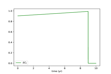
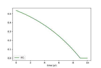
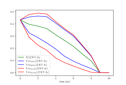
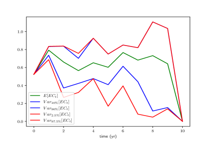
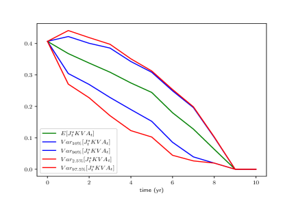
Figure 5.1: Plot of the deterministic maps $t\mapsto\widetilde{\rm EC}(t)$ [top left] and $t\mapsto\widetilde{\mathrm{KVA}}(t)$ [top right] corresponding to the static hedging case (5.10). Plots of mean (in green) and quantiles at levels 10% and 90% (in blue) and 2.5% and 97.5% (in red) of $\widehat{\rm EC}(t,\widetilde{S}_{t})$ in the delta hedging case without friction [Middle left] and in the delta hedging case with frictions [bottom left]. Plots of mean (in green) and quantiles at levels 10% and 90% (in blue) and 2.5% and 97.5% (in red) of $\widehat{\mathrm{KVA}}(t,\widetilde{S}_{t})$ in the delta hedging case without friction [Middle right] and in the delta hedging case with frictions [bottom right].

In particular, we obtain in the dynamic hedging case for the same numerical parameters as the ones used in Section 4.4, a confidence level $\alpha$ for the EC computations set at $99\%$, and a hurdle rate $r$ for the KVA computations set at 10%:

$$\begin{aligned} &\widehat{\rm HVA}^{\cdot}_{0}\simeq 0.095\mbox{ and }\widehat{\rm HVA}^{f}_{0}\simeq 0.046\mbox{, hence }\widehat{\rm HVA}_{0}\simeq 0.141,\\ &\widehat{\mathrm{KVA}}_{0}\simeq 0.407,\,\frac{\widehat{\mathrm{KVA}}_{0}}{\widehat{\rm HVA}_{0}}\simeq 2.881.\end{aligned}$$ (5.16)

As could be expected from Example 3.3 (see also Remark 3.3), there is ultimately less risk (as assessed by economic capital and KVA, cf. (3.11) and Figure 5.1) with the delta hedge than with the static, aka delta-vega hedge.

In the frictionless case $f=0$, we obtain by the same methodology

$$\begin{aligned} &\widehat{\rm HVA}_{0}=\widehat{\rm HVA}^{\cdot}_{0}\simeq 0.095,\\ &\widehat{\mathrm{KVA}}_{0}\simeq 0.433,\,\frac{\widehat{\mathrm{KVA}}_{0}}{\widehat{\rm HVA}_{0}}\simeq 4.550.\end{aligned}$$ (5.17)

By comparison with (5.16) (see also Figure 5.1), the dynamic hedging frictions happen to be slightly risk-reducing, meaning that the components $-pnl^{mtm}+{\rm HVA}^{mtm}_{(0)}=-pnl^{\cdot}+{\rm HVA}^{\cdot}_{(0)}$ and $f+{\rm HVA}^{f}_{(0)}$ of (5.1) tend to be negatively correlated in this case (for which we have no particular explanation).

6 Conclusion

6.1 Executive Summary (Encompassing Credit): A Global Valuation Framework

Accounting methods are also models in the sense of SR-11-7 (cf. https://www.federalres

erve.gov/supervisionreg/srletters/sr1107.htm) because they produce numbers, are based on assumptions, and have an impact on strategies. If they are misaligned with economics they cause a misalignement of interests between executives and shareholders. Hence, model risk is a concept that does not apply only to pricing models, but should be extended to accounting principles for dealer banks, including the specification of their CVA and FVA metrics (as these are liabilities to the bank, see Crépey (2022, Section 1) and Albanese et al. (2021, Figure 1)). From this model risk perspective, the CVA and FVA should be viewed as two additional “global trades” of the bank, deserving HVA in the same way as individual deals “$\cdot$” in the above. Introducing the cumulative counterparty default (resp. funding) losses $\mathcal{C}$ (resp. $\mathcal{F}$) of the CVA (resp. FVA) trading desk of the bank, the overall loss trading process of the bank accounting for the market, credit, funding, and dynamic hedging plus model risk (and dynamic hedging frictions) cash flows $\mathcal{M}$, $\mathcal{C},$ $\mathcal{F},$ and $\mathcal{H}$ is given by the martingale (compare with (5.3))

$$\begin{aligned} &\mathcal{L}=-(\mathcal{M}+{\rm MtM}_{(0)})+(\mathcal{C}+\mathrm{CVA}_{(0)})+(\mathcal{F}+\mathrm{FVA}_{(0)})+(\mathcal{H}+{\rm HVA}_{(0)}),\\ \end{aligned}$$ (6.1)

where MtM, CVA, FVA, and HVA are the fair valuation processes of $\mathcal{M}$, $\mathcal{C},$ $\mathcal{F}$ and $\mathcal{H}$ (including CVA and FVA analogs $\mathcal{H}^{cva}$ and $\mathcal{H}^{fva}$ of $\mathcal{H}^{\cdot}$ in (3.4)). In the model-risk-free and frictionless setup of Albanese et al. (2021) & Crépey (2022), $\mathcal{H}$ reduces to the frictionless dynamic hedging losses of the bank, naturally assumed to be a zero-valued martingale, hence ${\rm HVA}=va(\mathcal{H})=0$. In this paper, due to Darwinian model risk, $\mathcal{H}$ also incorporates model risk and market frictions. The ensuing process $\mathcal{H}$ is not a martingale anymore, whence a nontrivial hedging valuation adjustment ${\rm HVA}$. The resulting HVA can be seen as the bridge between a global fair valuation model and the local models used by the different desks of the bank. The HVA risk is then risk-adjusted by the KVA defined from (6.1) by (5.5)-(5.6). In particular, model risk is the channel through which market risk reintroduces itself into XVA computations (see the second paragraph of Section 1.1).

Remark 6.1.

Regarding its KVA computations, a bank could also be subject to Darwinian model risk: To enhance its competitiveness in the short term, a bank might be tempted to use a model understating the risk and economic capital of the bank. A sound practice in this regard is to combine different, equally valid (realistic and co-calibrated) models for simulating the set of trajectories underlying the economic capital and KVA computations (Albanese et al., 2023, Section 4.3). Such a Bayesian KVA approach typically fattens the tails of the simulated distributions and avoids under-stated risk estimates.

6.2 Take-Away Message: Bad Models Should Be Banned not Managed

A major step in the financial derivatives literature is the robustness result of Karoui, Jeanblanc-picqué, and Shreve (1998) according to which a convex position will be hedged conservatively with the Black-Scholes model as long as the volatility is overestimated. However, this assumes that the bank is a market maker in a position to impose its own (in this case overestimated) price for the claim at hand. In this paper we consider the opposite pattern where, due to the competition between banks, a trader can only sell the option at a price lower than its true value, hence losses for the bank (unless the trader uses the true model). In order to quantify the above, we revisit Burnett (2021) & Burnett and Williams (2021)’s notion of hedging valuation adjustment (HVA) in the direction of model risk. The fact evidenced by Example 3.3 that vega hedging may actually increase Darwinian model risk illustrates well that Darwinian model risk cannot be hedged. It can only be provisioned against or, preferably, compressed, by improving the quality of the models that are used by traders. In any case, a provision for model risk should be risk-adjusted. But, as the paper illustrates, a risk-adjusted reserve would be much greater than the “HVA uptick” (price difference) currently used in banks, by a factor 3 to 5 in our experiments (cf. Remark 3.2 and (5.16)-(5.17)), and it could be even more if one accounted for the price impact of a liquidation in extreme market conditions (cf. https://www.risk.net/derivatives/6556166/remembering-the-range-accrual-bloodbath effects already mentioned in Remark 2.4). Risk-adjusted HVA computations are also very demanding. In particular, beyond analytical toy examples such as the one of Section 5.4 (and already in the case of Section 5.5), HVA risk-adjusted KVA computations (starting with pathwise ${\rm HVA}^{f}$ computations) require dynamic recalibration in a simulation setup, for assessing the hedging ratios used by the traders at future time points as well as the time of explosion of the trader’s strategy (time of model switch $\tau_{s}^{\cdot}$). Hence, from the computational workload viewpoint too, the best practice would be that banks only rely on high-quality models, so that such computations are simply not needed.

To summarize, the orders of magnitude of the corrections that would be required for duly compensating model risk (accounting not only for misvaluation but also for the associated mishedge), as well as the corresponding computational burden for a precise assessment of the latter, suggest that bad models should not so much be managed via reserves, as excluded altogether.

Appendix A Pricing Equations in the Jump-to-Ruin Model

In this section we provide pricing analytics in the jr model (2.1) for $S$, with jump-to-ruin time (first jump time of $N$) $\theta$. We also consider the auxiliary Black-Scholes model

$$d\tilde{S}_{t}=\lambda\tilde{S}_{t}dt+\sigma\tilde{S}_{t}dW_{t},$$ (A.1)

starting from $\tilde{S}_{0}=S_{0}$, where $\lambda$ and $\sigma$ (omitted in the notation for $d_{\pm}$ below when clear from the context) were introduced after (2.1). Hence $S_{t}=\mathds{1}_{\{{N_{t}=0}\}}\tilde{S}_{t},\,t\geq 0.$ Given the maturity $T=\overline{T}$ and strike $K>0$ of an option, let, for every pricing time $t$ and stock value $S$,

$$\begin{aligned} d_{\pm}(t,S;\lambda,\sigma)=\frac{\ln(\frac{S}{K})+\lambda(T-t)}{\sigma\sqrt{T-t}}\pm\frac{1}{2}\sigma\sqrt{T-t}.\end{aligned}$$ (A.2)

We first consider the pricing of a vanilla call option.

Proposition A.1.

The jr value process (1.1)-(2.3) of the call option with payoff $(S_{T}-K)^{+}$ at time $T$ can be represented as

$$C^{jr}_{t}=u(t,S_{t})\mathds{1}_{[0,T)},\,t\in[0,T],$$

where the pricing function $u=u(t,S):={\mathbb{E}}\big{(}(S_{T}-K)^{+}\big{|}S_{t}=S\big{)}$ is the unique classical solution with linear growth in $S$ to the PDE

$$\left\{\begin{array}[]{l}u(T,S)=(S-K)^{+},\;S\geq 0\\ \partial_{t}u(t,S)+\lambda S\partial_{S}u(t,S)+\frac{{\sigma}^{2}S^{2}}{2}\partial^{2}_{S^{2}}u(t,S)-\lambda u(t,S)=0,\;t<T,\,S\geq 0.\end{array}\right.$$ (A.5)

For $t<T$,

$$\begin{aligned} C^{jr}_{t}=S_{t}\mathcal{N}(d_{+}(t,S_{t}))-Ke^{-\lambda(T-t)}\mathcal{N}(d_{-}(t,S_{t})).\end{aligned}$$ (A.6)

Proof.  We have $S_{T}=\mathds{1}_{\{\theta>T\}}\tilde{S}_{T}=\mathds{1}_{\{\theta>T\}}S_{0}\exp\left(\sigma W_{T}+(\lambda-\frac{\sigma^{2}}{2})T\right)$. Since $(S_{T}-K)^{+}=0$ on ${\theta\leq T}$ and $S_{T}=\tilde{S}_{T}$ on ${\theta>T},$ it follows that, on $\{t<\theta\}$,

$${\mathbb{E}}_{t}\left[(S_{T}-K)^{+}\right]={\mathbb{E}}_{t}\left[\mathds{1}_{\{\theta>T\}}(S_{T}-K)^{+}\right]=$$

$$={\mathbb{E}}_{t}\left[\mathds{1}_{\{\theta>T\}}(\tilde{S}_{T}-K)^{+}\right]={\mathbb{E}}_{t}\left[e^{-\lambda(T-\tau)}(\tilde{S}_{T}-K)^{+}\right],$$

by independence between $W$ and $N$ in (1.1). One recognizes the probabilistic expression for the time-$t$ price of the vanilla call option in the auxiliary Black-Scholes model (A.1), hence the proposition follows from standard Black-Scholes results.  

We now consider the pricing of a put option in the jr model, in two forms: either a vanilla put with payoff $(K-S_{T})^{+}$, or a vulnerable put with payoff $\mathds{1}_{\{\theta>T\}}(K-S_{T})^{+}$.

Proposition A.2.

The jr value process (1.1) of the vanilla put can be represented as

$$\begin{aligned} P^{jr}_{t}=v(t,S_{t})\mathds{1}_{[0,T)},\,t\in[0,T],\end{aligned}$$ (A.8)

where the vanilla put pricing function $v=v(t,S):={\mathbb{E}}\big{(}(K-S_{T})^{+}\big{|}S_{t}=S\big{)}$ is the unique bounded classical solution to the PDE

$$\left\{\begin{array}[]{l}v(T,S)=(K-S)^{+},\;S\geq 0\\ \partial_{t}v(t,S)+\lambda S\partial_{S}v(t,S)+\frac{{\sigma}^{2}S^{2}}{2}\partial^{2}_{S^{2}}v(t,S)\\ \;\;\;\;\;\;\;\;\;\;\;\;\;\;\;\;\;\;-\lambda v(t,S)+\lambda K=0,\;t<T,\,S\geq 0.\end{array}\right.$$ (A.12)

For $t<T$,

$$\begin{aligned} &P^{jr}_{t}=Ke^{-\lambda(T-t)}\mathcal{N}(-d_{-}(t,S_{t}))-S_{t}\mathcal{N}(-d_{+}(t,S_{t}))+K(1-e^{-\lambda(T-t)}).\end{aligned}$$ (A.13)

Proof.  Taking expectation in the decomposition $S_{T}-K=(S_{T}-K)^{+}-(S_{T}-K)^{-}$ yields the (model-free) call-put parity relationship

$$\begin{aligned} S_{t}-K=u(t,S_{t})-v(t,S_{t}),\,t\leq T,\end{aligned}$$ (A.14)

hence $v=u-(S-K)$, from which the PDE characterization based on (A.12) for $v$ results from the PDE characterization based on (A.5) for $u$. Moreover, we deduce from (A.6) that, for $t<T$,

$$P^{jr}_{t}=C^{jr}_{t}-(S_{t}-K)=S_{t}\left(\mathcal{N}(d_{+}(t,S_{t}))-1\right)-K\left(e^{-\lambda(T-t)}\mathcal{N}(d_{-}(t,S_{t}))-1\right)$$

$$=Ke^{-\lambda(T-t)}\mathcal{N}(-d_{-}(t,S_{t}))-S_{t}\mathcal{N}(-d_{+}(t,S_{t}))+K(1-e^{-\lambda(T-t)}),$$

which is (A.13).  

In accordance with (A.13):

Definition A.1.

For $t<\theta\wedge T$, given the observed spot price $S_{t}=S>0$, the Black-Scholes implied volatility $\Sigma_{t}=\Sigma(t,S)$ of the vanilla put in the jr model is the unique solution $\Sigma$ to

$$\begin{aligned} &Ke^{-\lambda(T-t)}\mathcal{N}(-d_{-}(t,S;\lambda,\sigma))-S\mathcal{N}(-d_{+}(t,S;\lambda,\sigma))+K(1-e^{-\lambda(T-t)})\\ &\;\;\;\;\;\;\;\;\;=K\mathcal{N}(-d_{-}(t,S;0,\Sigma_{t}))-S\mathcal{N}(-d_{+}(t,S;0,\Sigma_{t})).\end{aligned}$$ (A.15)

We also set $\Sigma(t,0)=0.\$

Remark A.1.

For $S=0$, any $\Sigma\geq 0$ solves (A.15): for any $\Sigma$, $d_{\pm}=-\infty$ as $\ln(\frac{0}{K})=-\infty$, so $K\mathcal{N}(-d_{-})-S\mathcal{N}(-d_{+})=K-S=K$ (for $S=0$).

Proposition A.3.

The value process (1.1) of the vulnerable put is given by

$$\begin{aligned} Q^{jr}_{t}&=\mathds{1}_{t<\theta\wedge T}\big{(}P^{jr}_{t}-(1-e^{-\lambda(T-t)})K\big{)}=\\ &\;\;\;\;\;\;\;\;\;\mathds{1}_{t<\theta\wedge T}\Big{(}Ke^{-\lambda(T-t)}\mathcal{N}\big{(}-d_{-}(t,S_{t})\big{)}-S_{t}\mathcal{N}\big{(}-d_{+}(t,S_{t})\big{)}\Big{)}.\end{aligned}$$ (A.16)

For $t<T$,

$$\begin{aligned} P^{jr}_{t}-Q^{jr}_{t}&=\mathds{1}_{t<\theta}K(1-e^{-\lambda(T-t)})+\mathds{1}_{t\geq\theta}K.\end{aligned}$$ (A.17)

Proof.  We have

$$\mathds{1}_{\{\theta>T\}}(S_{T}-K)=\mathds{1}_{\{\theta>T\}}\big{(}(S_{T}-K)^{+}-(S_{T}-K)^{-}\big{)},$$

which in jr reduces to

$$S_{T}-\mathds{1}_{\{\theta>T\}}K=(S_{T}-K)^{+}-\mathds{1}_{\{\theta>T\}}(S_{T}-K)^{-}.$$

By taking time-$t$ conditional expectations, we have, on $\{t<\theta\wedge T\}$, that $S_{t}-Ke^{-\lambda(T-t)}=C^{jr}_{t}-Q^{jr}_{t},$ which yields

$$\begin{aligned} Q^{jr}_{t}&=C^{jr}_{t}-S_{t}+Ke^{-\lambda(T-t)},\end{aligned}$$

out of which (still on $\{t<\theta\wedge T\}$) the first identity in (A.16) follows from (A.14) and the second identity in turn follows from (A.13). Besides, on $\{t\geq\theta\}$, we have $Q^{jr}=0$ and $P^{jr}=K$, whereas on $\{t\geq T\}$ we have $Q^{jr}=0$, which completes the proof of (A.16) and (A.17).  

Proposition A.4.

Setting $w(t,S)=v(t,S)-K(1-e^{-\lambda(T-t)})$ (see Proposition A.2 and (A.17)), the vulnerable put is replicable on $[0,\theta\wedge T]$ in the jr model (in the absence of model risk and hedging frictions), by the dynamic strategy $\zeta$ in $S$ and $\eta$ in the vanilla put given by

$$\begin{aligned} \zeta_{t}=-\frac{\mathcal{N}\big{(}-d_{+}(t,S_{t})\big{)}}{1-\mathcal{N}\big{(}-d_{-}(t,S_{t})\big{)}},\,\eta_{t}=-\frac{\mathcal{N}\big{(}-d_{-}(t,S_{t})\big{)}}{1-\mathcal{N}\big{(}-d_{-}(t,S_{t})\big{)}},\,t<{\tau_{s}}\wedge T,\end{aligned}$$ (A.18)

and the number of constant riskless assets deduced from the budget condition $w(t,S_{t})$ on the strategy.

Proof.  The profit-and-loss associated with the hedging strategy $\zeta$ in $S$ and $\eta$ in the vanilla put, both assumed left-limits of càdlàg processes, evolves following (the position being assumed to be unwound at $\theta$)

$$dpnl_{t}=\mathds{1}_{\{{t\leq\theta}\}}(dQ^{jr}_{t}-\zeta_{t}dS_{t}-\eta_{t}dP^{jr}_{t})$$

(with $pnl_{0}=0$). Itô formulas with (elementary) jump exploiting the results of Propositions A.2 and A.3 yield (cf. (2.1))

$$dpnl_{t}=\mathds{1}_{\{{t\leq\theta}\}}(\alpha_{t}dW_{t}+\beta_{t}dM_{t}),$$

where

$$\alpha_{t}=\sigma S_{t}\Big{(}\partial_{S}w(t,S_{t-})-\zeta_{t}-\eta_{t}\partial_{S}v(t,S_{t-})\Big{)},\,\beta_{t}=-w(t,S_{t-})+\zeta_{t}S_{t-}+\eta_{t}\big{(}v(t,S_{t-})-K\big{)}.$$

Hence the replication condition $\alpha=\beta=0$ reduces to the linear systems

$$\begin{aligned} &\partial_{S}w(t,S_{t-})-\zeta_{t}-\eta_{t}\partial_{S}v(t,S_{t-})=-w(t,S_{t-})+\zeta_{t}S_{t-}+\eta_{t}\big{(}v(t,S_{t-})-K\big{)}=0\end{aligned}$$ (A.19)

in the $(\zeta_{t},\eta_{t})$ (one system for each $t<{\tau_{s}}\wedge T$). Using (A.13) for the first line and (A.16) and (A.17) for the second line, one verifies that (A.18) solves (A.19).  

Appendix B Proof of Theorem 4.1

Lemma B.1.

Under Assumptions 4.2 and 4.6, there exists $C_{3}>0$ such that, for all ${\rm h}>0$ and $u\in\left\{\partial_{l}q^{\star},(\partial_{x}(\partial_{l}q^{\star})\sigma;1\leq l\leq d\right\}$,

$$\begin{aligned} &\sup_{0<t-s<{\rm h}}\mathbb{E}\left[\left|u(t,\mathcal{X}_{t})-u(s,\mathcal{X}_{s})\right|^{2}\right]^{\frac{1}{2}}\leq C_{3}{\rm h}^{\alpha}.\end{aligned}$$

Proof.  Since $1-\prod_{\jmath=1}^{L}\mathds{1}_{\{{\nu^{\jmath}_{t}=\nu^{\jmath}_{s}}\}}\leq\sum_{\jmath=1}^{L}(\nu^{\jmath}_{t}-\nu^{\jmath}_{s}),$ we have, for some constant $C\geq 0$ varying from line to line,

$$\begin{aligned} &\mathbb{E}\left[\left|u(t,\mathcal{X}_{t})-u(s,\mathcal{X}_{s})\right|^{2}\right]^{\frac{1}{2}}\\ &\leq\sqrt{2}\mathbb{E}\left[\left|u(t,X_{t},J_{t})-u(t,X_{t},J_{s})\right|^{2}\right]^{\frac{1}{2}}+\sqrt{2}\mathbb{E}\left[\left|u(t,X_{t},J_{s})-u(s,X_{s},J_{s})\right|^{2}\right]^{\frac{1}{2}}\\ &\leq C\left(\mathbb{E}\left[\left|u(t,X_{t},J_{t})-u(t,X_{t},J_{s})\right|^{2}\sum_{\jmath=1}^{L}(\nu^{\jmath}_{t}-\nu^{\jmath}_{s})\right]^{\frac{1}{2}}+(t-s)^{\alpha}+(t-s)^{\frac{1}{2}}\right)\\ &\leq C\left(\sum_{\jmath=1}^{L}\mathbb{E}\left[\int_{s}^{t}\lambda^{\jmath}_{r}dr\right]^{\frac{1}{2}}+(t-s)^{\alpha}\right)\leq C\left(L\sqrt{\Lambda(t-s)}+(t-s)^{\alpha}\right)\leq C_{3}{\rm h}^{\alpha},\end{aligned}$$

where we used equation (4.3) and the bound on the maps $\lambda^{\jmath}$.  

Coming to the proof of the theorem, we have, for $t=0$ for notational simplicity,

$$\begin{aligned} &\left|{\rm HVA}^{\rm h}_{0}-{\rm HVA}^{f}_{0}\right|=\left|\mathbb{E}\left[\sum_{i=1}^{n}\varphi^{\rm h}_{t^{\rm h}_{i}}\right]-\mathbb{E}\left[\int_{0}^{T^{\star}}\varphi_{t}dt\right]\right|\\ &=\left|\frac{\sqrt{{\rm h}}}{2}\mathbb{E}\left[\sum_{i=1}^{n}X^{\top}_{t^{\rm h}_{i}}{\rm\mathbf{k}}(\delta a_{t^{\rm h}_{i}})^{\mathrm{abs}}\right]-\frac{1}{\sqrt{2\pi}}\mathbb{E}\left[\sum_{i=1}^{n}\int_{t^{\rm h}_{i-1}}^{t^{\rm h}_{i}}X^{\top}_{t}{\rm\mathbf{k}}(\Gamma\sigma)^{\mathrm{abs}}(t,\mathcal{X}_{t})dt\right]\right|\\ &\leq\sum_{l=1}^{d}{\rm k}_{l}\left|\frac{\sqrt{{\rm h}}}{2}\mathbb{E}\left[\sum_{i=1}^{n}X^{l}_{t^{\rm h}_{i}}\left|a^{l}_{t^{\rm h}_{i}}-a^{l}_{t^{\rm h}_{i-1}}\right|\right]-\frac{1}{\sqrt{2\pi}}\mathbb{E}\left[\sum_{i=1}^{n}\int_{t^{\rm h}_{i-1}}^{t^{\rm h}_{i}}X^{l}_{t}|\partial_{x}(\partial_{l}q^{\star})\sigma|(t,\mathcal{X}_{t})dt\right]\right|\\ &={\rm h}\sum_{l=1}^{d}\sum_{i=1}^{n}{\rm k}_{l}\left|\mathbb{E}\left[\frac{1}{2\sqrt{{\rm h}}}X^{l}_{t^{\rm h}_{i}}\left|a^{l}_{t^{\rm h}_{i}}-a^{l}_{t^{\rm h}_{i-1}}\right|-\frac{1}{{\rm h}\sqrt{2\pi}}\int_{t^{\rm h}_{i-1}}^{t^{\rm h}_{i}}X^{l}_{t}|\partial_{x}(\partial_{l}q^{\star})\sigma|(t,\mathcal{X}_{t})dt\right]\right|\\ &\leq T^{\star}\sum_{l=1}^{d}{\rm k}_{l}\sup_{0\leq s<t\leq T^{\star},t-s={\rm h}}\left|\mathbb{E}\left[\frac{1}{2\sqrt{{\rm h}}}X^{l}_{t}\left|a^{l}_{t}-a^{l}_{s}\right|-\frac{1}{{\rm h}\sqrt{2\pi}}\int_{s}^{t}X^{l}_{u}|\partial_{x}(\partial_{l}q^{\star})\sigma|(u,\mathcal{X}_{u})du\right]\right|.\end{aligned}$$

We fix $1\leq l\leq d$ and we show that

$$\begin{aligned} \sup_{t-s={\rm h}}\left|\mathbb{E}\left[\frac{1}{2\sqrt{{\rm h}}}X^{l}_{t}\left|a^{l}_{t}-a^{l}_{s}\right|-\frac{1}{{\rm h}\sqrt{2\pi}}\int_{s}^{t}X^{l}_{u}|\partial_{x}(\partial_{l}q^{\star})\sigma|(u,\mathcal{X}_{u})du\right]\right|\rightarrow_{{\rm h}\rightarrow 0}0.\end{aligned}$$ (B.1)

In fact, for all $0\leq s<t\leq T^{\star}$ such that $t-s={\rm h}$,

$$\begin{aligned} &\left|\mathbb{E}\left[\frac{1}{2\sqrt{{\rm h}}}X^{l}_{t}\left|a^{l}_{t}-a^{l}_{s}\right|-\frac{1}{{\rm h}\sqrt{2\pi}}\int_{s}^{t}X^{l}_{u}|\partial_{x}(\partial_{l}q^{\star})\sigma|(u,\mathcal{X}_{u})du\right]\right|\\ &\leq\frac{1}{2\sqrt{{\rm h}}}\left|\mathbb{E}\left[(X^{l}_{t}-X^{l}_{s})\left|a^{l}_{t}-a^{l}_{s}\right|\right]\right|\\ &+\frac{1}{2\sqrt{{\rm h}}}\left|\mathbb{E}\left[X^{l}_{s}\left(\left|a^{l}_{t}-a^{l}_{s}\right|-\left|\partial_{x}(\partial_{l}q^{\star})\sigma(s,\mathcal{X}_{s})(W_{t}-W_{s})\right|\right)\right]\right|\\ &+\left|\mathbb{E}\left[\frac{1}{2\sqrt{{\rm h}}}X^{l}_{s}\left|\partial_{x}(\partial_{l}q^{\star})\sigma(s,\mathcal{X}_{s})(W_{t}-W_{s})\right|-\frac{1}{{\rm h}\sqrt{2\pi}}\int_{s}^{t}X^{l}_{u}|\partial_{x}(\partial_{l}q^{\star})\sigma|(u,\mathcal{X}_{u})du\right]\right|\\ \end{aligned}$$ (B.2)

Regarding the first term in the r.h.s. of (B.2), we have, by Assumption 4.2 and Lemma B.1,

$$\begin{aligned} &\frac{1}{2\sqrt{{\rm h}}}\left|\mathbb{E}\left[\left(X^{l}_{t}-X^{l}_{s}\right)\left|a^{l}_{t}-a^{l}_{s}\right|\right]\right|\leq\frac{1}{2\sqrt{{\rm h}}}\mathbb{E}\left[\left|X^{l}_{t}-X^{l}_{s}\right|^{2}\right]^{\frac{1}{2}}\mathbb{E}\left[\left|a^{l}_{t}-a^{l}_{s}\right|^{2}\right]^{\frac{1}{2}}\\ &\;\;\;\;\;\;\;\;\;\leq\frac{C_{1}}{2}{\rm h}^{-\frac{1}{2}+\frac{1}{2}+\alpha}=\frac{C_{1}}{2}{\rm h}^{\alpha}.\end{aligned}$$ (B.3)

We now consider the second term in the r.h.s. of (B.2). With $\delta\partial_{l}q^{\star}(t,x,j,k):=\partial_{l}q^{\star}(t,x,j)-\partial_{l}q^{\star}(t,x,k)$ and $C^{l}$ defined in (4.4), recalling that $|\delta\partial_{l}q^{\star}(t,x,j,k)|\leq C_{2}$ by Assumption 4.6, we compute by Itô’s formula:

$$\begin{aligned} &\frac{1}{2\sqrt{{\rm h}}}\left|\mathbb{E}\left[X^{l}_{s}\left(\left|a^{l}_{t}-a^{l}_{s}\right|-\left|\partial_{x}(\partial_{l}q^{\star})\sigma(s,\mathcal{X}_{s})(W_{t}-W_{s})\right|\right)\right]\right|\\ &\leq\frac{1}{2\sqrt{{\rm h}}}\mathbb{E}\left[X^{l}_{s}\int_{s}^{t}\left|(\partial_{t}+\mathcal{F})\partial_{l}q^{\star}(u,\mathcal{X}_{u})\right|du\right]+\sum_{\jmath=1}^{L}\frac{1}{2\sqrt{{\rm h}}}\mathbb{E}\left[X^{l}_{s}\left|\int_{s}^{t}\delta\partial_{l}q^{\star}(u,\mathcal{X}_{u},k)d\nu^{k}_{u}\right|\right]\\ &+\frac{1}{2\sqrt{{\rm h}}}\mathbb{E}\left[X^{l}_{s}\left|\int_{s}^{t}\left(\partial_{x}(\partial_{l}q^{\star})\sigma(u,\mathcal{X}_{u})-\partial_{x}(\partial_{l}q^{\star})\sigma(s,\mathcal{X}_{s})\right)dW_{u}\right|\right]\\ &\leq\frac{C^{l}}{2}\mathbb{E}\left[\int_{s}^{t}\left|(\partial_{t}+\mathcal{F})\partial_{l}q^{\star}(u,\mathcal{X}_{u})\right|^{2}du\right]^{\frac{1}{2}}+\frac{C_{2}}{2\sqrt{h}}\sum_{\jmath=1}^{L}\mathbb{E}\left[X^{l}_{s}(\nu^{\jmath}_{t}-\nu^{\jmath}_{s})\right]\\ &+\frac{C^{l}}{2\sqrt{{\rm h}}}\mathbb{E}\left[\int_{s}^{t}\left|\partial_{x}(\partial_{l}q^{\star})\sigma(u,\mathcal{X}_{u})-\partial_{x}(\partial_{l}q^{\star})\sigma(s,\mathcal{X}_{s})\right|^{2}du\right]^{\frac{1}{2}}\\ &\leq\frac{C^{l}C_{2}}{2}\sqrt{{\rm h}}+\frac{C^{l}C_{2}\Lambda L\sqrt{{\rm h}}}{2}+\frac{C^{l}C_{3}}{2}{\rm h}^{\alpha}\leq C{\rm h}^{\alpha},\end{aligned}$$ (B.4)

where we used

$$\begin{aligned} &\mathbb{E}\left[X^{l}_{s}(\nu^{\jmath}_{t}-\nu^{\jmath}_{s})\right]=\mathbb{E}\left[X^{l}_{s}\mathbb{E}_{s}\left[\nu^{\jmath}_{t}-\nu^{\jmath}_{s}\right]\right]=\mathbb{E}\left[X^{l}_{s}\int_{s}^{t}\lambda^{\jmath}_{u}du\right]\\ &\;\;\;\;\;\;\;\;\;\leq\mathbb{E}\left[\left(X^{l}_{s}\right)^{2}\right]^{\frac{1}{2}}\mathbb{E}\left[\left(\int_{s}^{t}\lambda^{\jmath}_{u}du\right)^{2}\right]^{\frac{1}{2}}\leq C^{l}\Lambda{\rm h},\\ &\mathbb{E}\left[\int_{s}^{t}\left|(\partial_{t}+\mathcal{F})\partial_{l}q^{\star}(u,\mathcal{X}_{u})\right|^{2}du\right]^{\frac{1}{2}}=\left(\int_{s}^{t}\mathbb{E}\left[\left|(\partial_{t}+\mathcal{F})\partial_{l}q^{\star}(u,\mathcal{X}_{u})\right|^{2}\right]du\right)^{\frac{1}{2}}\\ &\;\;\;\;\;\;\;\;\;\leq\sqrt{{\rm h}}\sup_{u\in[0,T^{\star}]}\mathbb{E}\left[\left|(\partial_{t}+\mathcal{F})\partial_{l}q^{\star}(u,\mathcal{X}_{u})\right|^{2}\right]^{\frac{1}{2}}\leq C_{2}\sqrt{{\rm h}},\end{aligned}$$

and Lemma B.1.

We finally deal with the last term in the r.h.s. of (B.2). As $\partial_{x}(\partial_{l}q^{\star})\sigma(s,\mathcal{X}_{s})\left(W_{t}-W_{s}\right)$ has, conditionally on $\mathfrak{F}_{s}$, the law $\mathcal{N}\left(0,{\rm h}\left|\partial_{x}(\partial_{l}q^{\star})\sigma(s,\mathcal{X}_{s})\right|^{2}\right)$, we have

$$\begin{aligned} \frac{1}{2\sqrt{{\rm h}}}\mathbb{E}\left[X^{l}_{s}\left|\partial_{x}(\partial_{l}q^{\star})\sigma(s,\mathcal{X}_{s})\left(W_{t}-W_{s}\right)\right|\right]&=\frac{1}{\sqrt{2\pi}}\mathbb{E}\left[X^{l}_{s}\left|\partial_{x}(\partial_{l}q^{\star})\sigma(s,\mathcal{X}_{s})\right|\right].\end{aligned}$$

We then obtain for this last term:

$$\begin{aligned} &\left|\mathbb{E}\left[\frac{1}{2\sqrt{{\rm h}}}X^{l}_{s}\left|\partial_{x}(\partial_{l}q^{\star})\sigma(s,\mathcal{X}_{s})\left(W_{t}-W_{s}\right)\right|-\frac{1}{{\rm h}\sqrt{2\pi}}\int_{s}^{t}X^{l}_{u}|\partial_{x}(\partial_{l}q^{\star})\sigma|(u,\mathcal{X}_{u})du\right]\right|\\ &=\frac{1}{\sqrt{2\pi}}\left|\mathbb{E}\left[X^{l}_{s}\left|\partial_{x}(\partial_{l}q^{\star})\sigma(s,\mathcal{X}_{s})\right|-\frac{1}{{\rm h}}\int_{s}^{t}X^{l}_{u}|\partial_{x}(\partial_{l}q^{\star})\sigma|(u,\mathcal{X}_{u})du\right]\right|\\ &\leq\frac{1}{\sqrt{2\pi}}\left|\mathbb{E}\left[X^{l}_{s}\left|\partial_{x}(\partial_{l}q^{\star})\sigma(s,\mathcal{X}_{s})\right|-\frac{1}{{\rm h}}\int_{s}^{t}X^{l}_{u}|\partial_{x}(\partial_{l}q^{\star})\sigma|(u,X_{u},J_{s})du\right]\right|\\ &+\frac{1}{{\rm h}\sqrt{2\pi}}\left|\mathbb{E}\left[\int_{s}^{t}X^{l}_{u}\left(|\partial_{x}(\partial_{l}q^{\star})\sigma|(u,X_{u},J_{s})-|\partial_{x}(\partial_{l}q^{\star})\sigma|(u,X_{u},J_{u})\right)du\right]\right|\\ &\leq\frac{1}{\sqrt{2\pi}}\left|\mathbb{E}\left[X^{l}_{s}|\partial_{x}(\partial_{l}q^{\star})\sigma(s,\mathcal{X}_{s})|-X^{l}_{r}|\partial_{x}(\partial_{l}q^{\star})\sigma(r,X_{r},J_{s})|\right]\right|\\ &+\frac{C^{l}}{\sqrt{{\rm h}2\pi}}\mathbb{E}\left[\int_{s}^{t}\left(\partial_{x}(\partial_{l}q^{\star})\sigma(u,X_{u},J_{s})-\partial_{x}(\partial_{l}q^{\star})\sigma(u,X_{u},J_{u})\right)^{2}du\sum_{\jmath=1}^{L}(\nu^{\jmath}_{t}-\nu^{\jmath}_{s})\right]^{\frac{1}{2}},\\ \end{aligned}$$

where the (random) $r\in(s,t)$ in the next-to-last line is obtained via the mean value theorem. We have, for a constant $C$ changing from term to term,

$$\begin{aligned} &\left|\mathbb{E}\left[X^{l}_{s}|\partial_{x}(\partial_{l}q^{\star})\sigma(s,\mathcal{X}_{s})|-X^{l}_{r}|\partial_{x}(\partial_{l}q^{\star})\sigma(r,X_{r},J_{s})|\right]\right|\\ &\leq\mathbb{E}\left[|X^{l}_{s}-X^{l}_{r}||\partial_{x}(\partial_{l}q^{\star})\sigma(s,\mathcal{X}_{s})|\right]+\mathbb{E}\left[X^{l}_{r}|\partial_{x}(\partial_{l}q^{\star})\sigma(s,\mathcal{X}_{s})|-\partial_{x}(\partial_{l}q^{\star})\sigma(r,X_{r},J_{s})|\right]\\ &\leq C_{1}h^{\frac{1}{2}}\sup_{t\in[0,T^{\star}]}\mathbb{E}\left[|\partial_{x}(\partial_{l}q^{\star})\sigma(t,\mathcal{X}_{t})|^{2}\right]^{\frac{1}{2}}+C{\rm h}^{\alpha}\mathbb{E}\left[X^{l}_{r}\right]+C\mathbb{E}\left[X^{l}_{r}|X_{r}-X_{s}|\right]\leq Ch^{\alpha},\end{aligned}$$ (B.5)

as

$$\begin{aligned} \sup_{t\in[0,T^{\star}]}\mathbb{E}\left[|\partial_{x}(\partial_{l}q^{\star})\sigma(t,\mathcal{X}_{t})|^{2}\right]^{\frac{1}{2}}\leq C(T^{\star})^{\alpha}+C^{l}+C\max_{1\leq\jmath\leq L}|\partial_{x}(\partial_{l}q^{\star})\sigma(0,0,k)|<\infty.\end{aligned}$$

Finally,

$$\begin{aligned} &\frac{C^{l}}{\sqrt{{\rm h}2\pi}}\mathbb{E}\left[\int_{s}^{t}\left(\partial_{x}(\partial_{l}q^{\star})\sigma(u,X_{u},J_{s})-\partial_{x}(\partial_{l}q^{\star})\sigma(u,X_{u},J_{u})\right)^{2}du\sum_{\jmath=1}^{L}(\nu^{\jmath}_{t}-\nu^{\jmath}_{s})\right]^{\frac{1}{2}}\\ &\frac{C^{l}C_{2}}{\sqrt{2\pi}}\mathbb{E}\left[\sum_{\jmath=1}^{L}\int_{s}^{t}\lambda^{\jmath}_{u}du\right]^{\frac{1}{2}}\leq\frac{C^{l}C_{2}}{\sqrt{2\pi}}\sqrt{L\Lambda{\rm h}}.\end{aligned}$$ (B.6)

Using (B.3)-(B.4)-(B.5)-(B.6), we obtain, for some constant $C\geq 0$,

$$\begin{aligned} \sup_{t-s={\rm h}}\left|\mathbb{E}\left[\frac{1}{2\sqrt{{\rm h}}}X^{l}_{t}\left|a^{l}_{t}-a^{l}_{s}\right|-\frac{1}{{\rm h}\sqrt{2\pi}}\int_{s}^{t}X^{l}_{u}|\partial_{x}(\partial_{l}q^{\star})\sigma|(u,\mathcal{X}_{u})doe\right]\right|\leq C{\rm h}^{\alpha},\end{aligned}$$

which proves (B.1) and therefore the theorem.

Appendix C Neural Nets Regression and Quantile Regressions for the Pathwise HVA^f, EC, and KVA of Section 5.5

The setup and notation are the ones of Section 5.5.

C.1 HVA^f Computations

The function $\widetilde{\rm HVA}^{f}$ in (5.15) is such that $\widetilde{\rm HVA}^{f}(T,\cdot)=0$, $\widetilde{\rm HVA}^{f}(t,0)=0$ for all $t$ and, for $u<t$ and $S\in(0,\infty)$,

$$\begin{aligned} \widetilde{\rm HVA}^{f}(u,S)&=\mathbb{E}\left[(f_{t}-f_{u})+\widetilde{\rm HVA}^{f}(t,S_{t})\,\middle|\,S_{u}=S\right]\\ &=\mathbb{E}\left[(f_{t}-f_{u})+\widetilde{\rm HVA}^{f}(t,S_{t})\mathds{1}_{\{{S_{t}>0}\}}\,\middle|S_{u}=S\right],\end{aligned}$$ (C.1)

for $f$ as per (4.10). Accordingly, we approximate on $(0,\infty)$ the functions $\widetilde{\rm HVA}^{f}(t_{i},\cdot)$ for $t_{i}:=i\frac{T}{10}$, as follows. Set $\widehat{\rm HVA}^{f}(t_{10},\cdot)=0$ and assume that we have already trained neural networks $\widehat{\rm HVA}^{f}(t_{k},\cdot)$, $i+1\leq k<10$. Based on sampled data

$$(X,Y)=\left(\widetilde{S}^{m}_{t_{i}},(f_{t_{i+1}}-f_{t_{i}})^{m}+\widehat{\rm HVA}^{f}(t_{i+1},S^{m}_{t_{i+1}})\mathds{1}_{\{{S^{m}_{t_{i+1}}>0}\}}\right)_{1\leq m\leq M},$$

where each $S^{m}_{t_{i+1}}$ is a obtained from (2.1) with initial condition $S^{m}_{t_{i}}=\widetilde{S}^{m}_{t_{i}}>0$ simulated from (A.1), in view of (C.1) and of the least-squares characterization of conditional expectation (in square integrable cases), we seek for $\widehat{\rm HVA}^{f}(t_{i},\cdot)$ in

$$\begin{aligned} \operatorname{argmin}_{u\in\mathcal{N}\!\mathcal{N}}\sum_{m=1}^{M}\left(\widehat{\rm HVA}^{f}(t_{i+1},S^{m}_{t_{i+1}})\mathds{1}_{\{{S^{m}_{t_{i+1}}>0}\}}+\left(f_{t_{i+1}}-f_{t_{i}}\right)^{m}-u(\widetilde{S}^{m}_{t_{i}})\right)^{2},\end{aligned}$$ (C.2)

where $\mathcal{N}\!\mathcal{N}$ denotes the set of feedforward neural networks with three hidden layers of 10 neurons each and ReLU activation functions.

We then obtain $\widehat{\rm HVA}^{f}(0,S_{0}){=0.04613}$ from $f_{t_{1}}+\widehat{\rm HVA}^{f}(t_{1},S_{t_{1}})$ as a sample mean. The corresponding standard deviation, $95\%$ confidence interval and relative error at $95\%$ are $\hat{\sigma}^{f}\simeq 6\times 10^{-3}$, $[0.04601,0.04624]$ and $\frac{1.96\hat{\sigma}^{f}}{\widehat{\rm HVA}^{f}_{0}\sqrt{M}}\simeq 0.25\%$, where $\hat{\sigma}^{f}$ denotes the empirical standard deviation of $f_{1}+\widehat{\rm HVA}^{f}(t_{1},S_{t_{1}})$.

C.2 EC Computations

Next we approximate $\widetilde{\rm EC}(t,\cdot)$ on $(0,\infty)$ by the two-stage scheme of Barrera et al. (2022, Section 4.3), for each $t=t_{i},1\leq i<10$. Recall $t^{\prime}=(t+1)\wedge T$. We first train a neural network $\widehat{\mathbb{V}}a\mathbb{R}(t,\cdot)$ approximating $\widetilde{\mathbb{V}}a\mathbb{R}(t,\cdot)$ based on sampled data $(X,Y)=\left(\widetilde{S}^{m}_{t},\left(\mathcal{L}_{t^{\prime}}-\mathcal{L}_{t}\right)^{m}\right)_{1\leq m\leq M}$ and on the pinball-type loss $(y-u(x))^{+}+(1-\alpha)u(x)$, i.e. we seek for $\widehat{\mathbb{V}}a\mathbb{R}(t,\cdot)$ in

$$\operatorname{argmin}_{u\in\mathcal{N}\!\mathcal{N}}\frac{1}{M}\sum_{m=1}^{M}\left(\left(\mathcal{L}_{t^{\prime}}-\mathcal{L}_{t}\right)^{m}-u(\widetilde{S}^{m}_{t})\right)^{+}+(1-\alpha)u(\widetilde{S}^{m}_{t}).$$

Note from (5.1) that, for $t=t_{i}$, sampling $\mathcal{L}_{t^{\prime}}-\mathcal{L}_{t}$ uses the already trained neural network $\widehat{\rm HVA}^{f}(t_{i+1},\cdot)$. For $t=1yr$ (where the approximation should be the worst due to error accumulated on $\widetilde{\rm HVA}^{f}$ from dynamic programming), the Monte Carlo estimate of Barrera et al. (2022, (4.10)) for the distance in $p$-values between the estimate $\widehat{\mathbb{V}}a\mathbb{R}(t,S_{t})$ and the targeted (unknown) $\mathbb{V}a\mathbb{R}_{t}\left(\mathcal{L}_{t^{\prime}}-\mathcal{L}_{t}\right)$ is less than $3.6\times 10^{-3}\leq 1-\alpha=10^{-2}$ with 95% probability.

We then train neural networks $\widehat{\rm EC}(t,\cdot)$ approximating $\widetilde{\rm EC}(t,\cdot)$ on $(0,\infty)$ at times $t=t_{i}$ based on sampled data $(X,Y)=\left(\widetilde{S}^{m}_{t},(\mathcal{L}_{t^{\prime}}-\mathcal{L}_{t})^{m}\right)_{1\leq m\leq M}$ and on the loss

$$\left((1-\alpha)^{-1}(y-\widehat{\mathbb{V}}a\mathbb{R}(t,x))^{+}+\widehat{\mathbb{V}}a\mathbb{R}(t,x)-u(x)\right)^{2},$$

i.e. we seek for $\widehat{\rm EC}(t,\cdot)$ in

$$\operatorname{argmin}_{u\in\mathcal{N}\!\mathcal{N}}\frac{1}{M}\sum_{m=1}^{M}\left((1-\alpha)^{-1}\left(\left(\mathcal{L}_{t^{\prime}}-\mathcal{L}_{t}\right)^{m}-\widehat{\mathbb{V}}a\mathbb{R}(S^{m}_{t})\right)^{+}+\widehat{\mathbb{V}}a\mathbb{R}(S^{m}_{t})-u(x)\right)^{2}.$$

For $t=1yr$, the Monte Carlo estimate of Barrera et al. (2022, (4.8)) for the $L_{2}$-norm of the difference between the estimate $\widehat{\rm EC}(t,\widetilde{S}_{t})$ and the targeted (unknown) $\widetilde{\rm EC}(t,\widetilde{S}_{t})$ is smaller than $0.067$ (itself significantly less then the orders of magnitude of EC visible on the left panels of Figure 5.1) with probability $95\%$.

We also compute $\widehat{\mathbb{V}}a\mathbb{R}(0,S_{0})=0.0120$ (which is needed for $\widehat{\rm EC}(0,S_{0})$ below) as an empirical (unconditional) value-at-risk. The corresponding $95\%$ confidence interval and relative error at $95\%$ are $[0.0117,0.0123]$ and $\frac{1.96}{\widehat{\mathbb{V}}a\mathbb{R}(0,S_{0})\hat{d}(\widehat{\mathbb{V}}a\mathbb{R}(0,S_{0}))}\sqrt{\frac{\alpha(1-\alpha)}{M}}\simeq 2.3\%$, where $\hat{d}$ denotes the empirical density of $\mathcal{L}_{t_{1}}-\mathcal{L}_{t_{0}}$. Finally we compute $\widehat{\rm EC}(0,S_{0})=0.493$ using the recursive algorithm of Costa and Gadat (2021, Eqn (4)). Using the central limit theorem for expected shortfalls derived in Costa and Gadat (2021, Theorem 1.3), a $95\%$ confidence interval is $[0.451,0.534]$ and the relative error at $95\%$ is $\sqrt{\frac{b_{M}}{2}}\frac{1.96\hat{\sigma}^{s}}{(1-\alpha)\widehat{\rm EC}(0,S_{0})}\simeq 0.08$, where $\hat{\sigma}^{s}$ denotes the empirical standard deviation of $(\mathcal{L}_{1}-\mathcal{L}_{0})\mathds{1}_{\{{(\mathcal{L}_{1}-\mathcal{L}_{0})>\widehat{\mathbb{V}}a\mathbb{R}(0,S_{0})}\}}$ and $b_{M}$ is defined in Costa and Gadat (2021, Assumption $H_{a_{n},b_{n}}$).

C.3 KVA Computations

Last, we approximate $\widetilde{\mathrm{KVA}}(t,\cdot)$ at times $t=t_{i}$ on $(0,\infty)$, for $i$ decreasing from 10 to 1, by neural networks $\widehat{\mathrm{KVA}}(t_{i},\cdot)$, based on the following dynamic programming equation, for $0\leq i<10$:

$$\begin{aligned} \mathrm{KVA}_{t_{i}}&=\mathbb{E}_{t_{i}}\left[\mathrm{KVA}_{t_{i+1}}+h\int_{t_{i}}^{t_{i+1}}\left({\rm EC}_{u}-\mathrm{KVA}_{u}\right)^{+}du\right]\\ &\approx\mathbb{E}_{t_{i}}\left[\mathrm{KVA}_{t_{i+1}}+h(t_{i+1}-t_{i})\left({\rm EC}_{t_{i+1}}-\mathrm{KVA}_{t_{i+1}}\right)^{+}\right].\end{aligned}$$

Starting from $\widehat{\mathrm{KVA}}({t_{n}},\cdot)=0$ and having already trained the $\widehat{\mathrm{KVA}}({t_{j}},\cdot),j>i>0$, we train $\widehat{\mathrm{KVA}}({t_{i}},\cdot)$ based on sampled data

$$\begin{aligned} (X,Y)=&\left(\widetilde{S}^{m}_{t_{i}},h(t_{i+1}-t_{i})\left(\widehat{\rm EC}(t_{i+1},S^{m}_{t_{i+1}})-\widehat{\mathrm{KVA}}(t_{i+1},S^{m}_{t_{i+1}})\mathds{1}_{\{{S^{m}_{t_{i+1}}>0}\}}\right)^{+}\right.\\ &\hskip 28.45274pt\left.+\widehat{\mathrm{KVA}}(t_{i+1},S^{m}_{t_{i+1}})\mathds{1}_{\{{S^{m}_{t_{i+1}}>0}\}}\right)_{1\leq m\leq M}\end{aligned}$$

and on the quadratic loss $(y-u(x))^{2}$. We then compute $\widehat{\mathrm{KVA}}(0,S_{0})=0.407$ from $r(t_{1}-t_{0})(\widehat{\rm EC}(t_{1},S_{t_{1}})-\widehat{\mathrm{KVA}}(t_{1},S_{t_{1}})\mathds{1}_{\{{S_{t_{1}}>0}\}})+\widehat{\mathrm{KVA}}({t_{1}},S_{t_{1}})$ as a sample mean. The corresponding standard deviation, $95\%$ confidence interval and relative error at $95\%$ are $\hat{\sigma}^{kva}\simeq 6\times 10^{-2}$, $[0.4056,0.4082]$ and $\frac{1.96\hat{\sigma}^{kva}}{\widehat{\mathrm{KVA}}_{0}\sqrt{M}}\simeq 0.0028$, where $\hat{\sigma}^{kva}$ denotes the empirical standard deviation of $r(t_{1}-t_{0})(\widehat{\rm EC}(t_{1},S_{t_{1}})-\widehat{\mathrm{KVA}}(t_{1},S_{t_{1}})\mathds{1}_{\{{S_{t_{1}}>0}\}})+\widehat{\mathrm{KVA}}({t_{1}},S_{t_{1}})$.

References

- Albanese et al. (2021) Albanese, C., S. Crépey, R. Hoskinson, and B. Saadeddine (2021). XVA analysis from the balance sheet. Quantitative Finance 21(1), 99–123.
- Albanese et al. (2021) Albanese, C., S. Crépey, and S. Iabichino (2021). A Darwinian theory of model risk. Risk Magazine, July pages 72–77.
- Albanese et al. (2023) Albanese, C., S. Crépey, and S. Iabichino (2023). Quantitative reverse stress testing, bottom-up. Quantitative Finance 23(5), 863–875.
- Artzner et al. (2022) Artzner, P., K.-T. Eisele, and T. Schmidt (2022). Insurance-finance arbitrage. arXiv:2005.11022.
- Barrera et al. (2022) Barrera, D., S. Crépey, E. Gobet, H.-D. Nguyen, and B. Saadeddine (2022). Learning the value-at-risk and expected shortfall. arXiv:2209.06476.
- Barrieu and Scandolo (2015) Barrieu, P. and G. Scandolo (2015). Assessing financial model risk. European Journal of Operational Research 242(2), 546–556.
- Bartl et al. (2021) Bartl, D., S. Drapeau, J. Obloj, and J. Wiesel (2021). Sensitivity analysis of Wasserstein distributionally robust optimization problems. Proceedings of the Royal Society A 477(2256), 20210176.
- Benezet et al. (2022) Benezet, C., S. Crépey, and D. Essaket (2022). Hedging valuation adjustment for callable claims. arXiv:2304.02479.
- Bichuch et al. (2020) Bichuch, M., A. Capponi, and S. Sturm (2020). Robust XVA. Mathematical Finance 30(3), 738–781.
- Burnett (2021) Burnett, B. (2021). Hedging value adjustment: Fact and friction. Risk Magazine, February 1–6.
- Burnett and Williams (2021) Burnett, B. and I. Williams (2021). The cost of hedging XVA. Risk Magazine, April.
- Cont (2006) Cont, R. (2006). Model uncertainty and its impact on the pricing of derivative instruments. Mathematical Finance 16(3), 519–547.
- Costa and Gadat (2021) Costa, M. and S. Gadat (2021). Non asymptotic controls on a recursive superquantile approximation. Electronic Journal of Statistics 15(2), 4718–4769.
- Crépey (2013) Crépey, S. (2013). Financial Modeling: A Backward Stochastic Differential Equations Perspective. Springer Finance Textbooks.
- Crépey (2022) Crépey, S. (2022). Positive XVAs. Frontiers of Mathematical Finance 1(3), 425–465.
- Detering and Packham (2016) Detering, N. and N. Packham (2016). Model risk of contingent claims. Quantitative Finance 16(9), 1357–1374.
- Elices and Giménez (2013) Elices, A. and E. Giménez (2013). Applying hedging strategies to estimate model risk and provision calculation. Quantitative Finance 13(7), 1015–1028.
- Élie (2006) Élie, R. (2006). Contrôle stochastique et méthodes numériques en finance mathématique. Ph. D. thesis, University Paris-Dauphine. https://pastel.archives-ouvertes.fr/tel-00122883/file/thesis.pdf.
- European Parliament (2013) European Parliament (2013). Regulation (EU) No 575/2013 of the European Parliament and of the Council of 26 June 2013 on prudential requirements for credit institutions and investment firms and amending Regulation (EU) No 648/2012. Official Journal of the European Union 59(June 2013).
- European Parliament (2016) European Parliament (2016). Commission Delegated Regulation (EU) 2016/101 of 26 October 2015 supplementing Regulation (EU) No 575/2013 of the European Parliament and of the Council with regard to regulatory technical standards for prudent valuation under Article 105(14). Official Journal of the European Union 59(28 January 2016).
- Farkas et al. (2020) Farkas, W., F. Fringuellotti, and R. Tunaru (2020). A cost-benefit analysis of capital requirements adjusted for model risk. Journal of Corporate Finance 65, 101753.
- Kabanov and Safarian (2009) Kabanov, Y. and M. Safarian (2009). Markets with transaction costs: Mathematical Theory. Springer Science & Business Media.
- Karoui et al. (1998) Karoui, N. E., M. Jeanblanc-picqué, and S. E. Shreve (1998). Robustness of the Black and Scholes Formula. Mathematical Finance 8(2), 93–126.
- Silotto et al. (2021) Silotto, L., M. Scaringi, and M. Bianchetti (2021). Everything you always wanted to know about XVA model risk but were afraid to ask. arXiv:2107.10377.
- Singh and Zhang (2019a) Singh, D. and S. Zhang (2019a). Distributionally robust XVA via Wasserstein distance. Part 2: Wrong way funding risk. arXiv:1910.03993.
- Singh and Zhang (2019b) Singh, D. and S. Zhang (2019b). Distributionally robust XVA via Wasserstein distance: Wrong way counterparty credit and funding risk. arXiv:1910.01781.