A scalable and flexible Cox proportional hazards model for high-dimensional survival prediction and functional selection

Abstract

Cox proportional hazards model is one of the most popular models in biomedical data analysis. There have been continuing efforts to improve the flexibility of such models for complex signal detection, for example, via additive functions. Nevertheless, the task to extend Cox additive models to accomodate high-dimensional data is nontrivial. When estimating additive functions, commonly used group sparse regularization may introduce excess smoothing shrinkage on additive functions, damaging predictive performance. Moreover, an “all-in-all-out” approach makes functional selection challenging to answer if nonlinear effects exist. We develop an additive Cox PH model to address these challenges in high-dimensional data analysis. Notably, we impose a novel spike-and-slab LASSO prior that motivates the bi-level functional selection on additive functions. A scalable and deterministic algorithm, EM-Coordinate Descent, is designed for scalable model fitting. We compare the predictive and computational performance against state-of-the-art models in simulation studies and metabolomics data analysis. The proposed model is broadly applicable to various fields of research, e.g. genomics and population health, via freely available R package BHAM (https://boyiguo1.github.io/BHAM/)

Keywords Cox Model; Spike-and-Slab; Scalable; Machine Learning; Additive Models;

1 Introduction

Cox proportional hazards model (Cox model hereafter) is one of the most popular analytic choices to analyze right-censored time-to-event data. Cox model describes the change of risk, modeled as hazard, on the multiplicative scale and provides easily interpretable insights in disease etiology. When a variable enters the Cox model as a predictors, an implicit assumption is imposed: the effect of the predictor are linear. The linear assumption is restrictive and doubtful in many case. A viable solution is to replace each variable with its functional form such that the modified Cox model retains its interpretability while gaining flexibility to model complex signals. The Cox model with additive components (hereafter referred to as Cox additive model or CAM for short) has many successful applications in biomedical research, for example, dose-response curve modeling [1], disease progrognostic [2] to name a few. To clarify, the Cox additive model differs from the additive hazards model [3] even both models leverage additive functions of predictors. The two models answer different scientific questions: the Cox additive model measures hazard change on the multiplicative scale and produces risk ratio interpretation; the additive hazards model measures hazard change on the additive scale and produces risk difference interpretation. In this manuscript, we limit our focus to the Cox additive model, and defer interested readers to [4] for a review of the additive hazards model.

Splines function are one of the most popular choices for additive functions in CAM, because they are mathematically simple, smooth across the range, and hence provide easy interpretation. Mathematically, a spline funciton is a piece-wise polynomial function with continuity conditions imposed on the function. [5] To apply spline functions in CAM, one can easily replace each predictor with the matrix form of its corresponding spline function which is known. The estimation of coefficients follows the same procedure as fitting an ordinary Cox model. This approach is called regression spline. Nevertheless, if spline functions are overparameterized, i.e. using more than necessary degree of smoothness, regression spline models incline to be overfitted and the estimated functions are very wiggly. To make data-driven decision on the degrees of smoothness, smoothing penalty are applied, resulting the smoothing spline model [6].

Large volumes of biomedical data motivate the development of high-dimensional statistics. Here, we define high-dimensional statistics as the analytic models to address analyses where the number of predictors/dimensions is close, if not more than, the sample size ($p>>n$), commonly seen in -omics data and high-resolution image data. There have been sustaining efforts to extend Cox model to accommodate high-dimensional setting [7, 8, 9, 10, 11, 12], with a few allowing a small subset of predictors to be modeled nonparametrically[13] (also known semiparametric regression). The semiparametric regression approaches improve the flexibility of high-dimensional Cox models, but the improvement can be limited when the knowledge about predictors’ linearity is lacking, for example during the exploratory data analysis of genomics studies. A nonparametric regression approach is highly sought-after for full flexibility and autonomy.

A technical gap exists when attempting to extend the semiparametric regression to the nonparametric regression under the Cox proportional hazard framework for high-dimensional data analysis. Semiparametric regressions assume all additive functions included are necessary and only address the smoothing of these functions. This strategy would fail when applied to nonparametric regressions, as the selection of additive functions are necessary. In other words, under the nonparametric setting, one needs to address the sparsity of additive functions in addition to the smoothness of effective functions. One school of thoughts is to employ group sparse penalty on the coefficients of additive functions: [14] proposed a functional analogue of LASSO penalty;[15] proposed to uses SCAD penalties to selecting non-parametric component functions;[16] proposed a feature screening procedure for the additive cox model. These proposals can serve as effective variable selection tools, but are susceptible to inaccurate risk prediction. When constructing model penalty, function smoothness are not considered. Such strategies are not recommended in the high-dimensional generalized additive model literature, as models are prone to wiggle estimations when underlying signal is smooth. [17] In addition, these globally penalized models ignore the fact that each additive function can have different degrees of smoothness, and hence introduce an over-smoothed solution. [18] There are also other approaches provides flexible solutions to model survival outcome in the high-dimensional setting. [19] proposed to model survival outcome with piece-wise exponential models, which is based on the idea of fit a Poisson GLM with transformed survival outcomes. Nevertheless, this method is not computationally efficient and vulnerable to convergence problem due to the numeric calculations. [20] extended the trend filtering model to the survival setting. The solution is a series of step functions, which would not be optimal if underlying functions are assumed to be smooth.

In this article, we introduce the two-part spike-and-slab LASSO (SSL) prior for smooth functions [21] to the high-dimensional Cox additive model literature. Specially, the two-part SSL prior simultaneously addresses signal sparsity and function smoothness by allowing separate adaptive shrinkages on linear and nonlinear components of additive functions. Built upon the premise that better signal estimation produce better outcome prediction, we adopt the smoothing penalty concept via design matrix reparameterization to encourage accurate function estimation. In addition, the two-part SSL prior motivates the bi-level functional selection. Here, we define the bi-level selection as the decision-making on if a variable should be included in the model and if the variable has linear versus nonlinear effect. To the best of our knowledge, we are the first to apply spike-and-slab LASSO prior in the context of high-dimensional Cox additive model for the purposes of simultaneous survival prediction and functional selection. Meanwhile, fitting a Bayesian hierarchical model for high-dimensional data can be computationally intimidating. Hence, we develop a scalable EM-Coordinate Descent algorithm and provide user-friendly implementation in the open-source software environment R[22]. The implementation is freely available via https://github.com/boyiguo1/BHAM. The proposed framework contributes a flexible and efficient solution to high-dimensional molecular and clinical data analysis.

2 Cox Proportional Hazards Additive Model

For each individual indexed with $i$, we collect the the covariate variables $\boldsymbol{X}_{i}=(X_{i1},\dots,X_{ij})\in\mathbb{R}^{p}$ and the survival outcome $(T_{i},D_{i})\in\{\mathbb{R}^{+}\times\{0,1\}\}$ where $T_{i}$ is the observed survival time, and $D_{i}$ is a binary censoring indicator. $D_{i}$ takes the value 1 when the event of interest happens at the survival time $T_{i}$, and takes the value 0 when censoring happens. We assume non-informative right censoring, no competing risk or multiple occurrence of the event. The Cox proportional hazards model with additive functions $B_{j}(x_{j})=\boldsymbol{\beta}_{j}\boldsymbol{X}_{j}$ is formulated as

$$h(t_{i}|\boldsymbol{x}_{i})=h_{0}(t_{i})exp(\sum\limits^{p}_{j=1}B_{j}(x_{ij}))=h_{0}(t_{i})\exp(\sum\limits^{p}_{j=1}\boldsymbol{\beta}^{T}_{j}\boldsymbol{X}_{ij}).$$

For the purpose of identifiability, we impose an constraint on each additive function such that $E[B_{j}(x_{j})]=0$. $h(t_{i})$ is the hazard function and $h_{0}(t_{i})$ is the baseline hazard function. The hazard function $h(t)$ describes the instantaneous rate of event occurrence among people who are still at risk at the moment. To note, different from GLMs, there is no intercept term necessary as the baseline hazard function $h_{0}(t)$ estimates an reference level of survival risk. We defer to [23, 24] for full treatment of Cox proportional hazards models.

We consider maximizing the partial log-likelihood function [25] for Cox model fitting, mathematically,

$$pl(\boldsymbol{\beta})=\sum\limits^{n}_{i=1}d_{i}\log\frac{\exp{\boldsymbol{x}_{i}\boldsymbol{\beta}}}{\sum_{j\in R(t_{i})}\exp(\boldsymbol{x}_{j}\boldsymbol{\beta})},$$ (1)

where $R(t_{i})$ denotes the risk set at time $t_{i}$, i.e. the set of all patients who still survived prior to time $t_{i}$. When tied failure or censoring time exists, a modified partial log-likelihood function can be used [26]. Conditional on $\boldsymbol{\beta}$, the baseline hazard function $h_{0}(t_{i})$ can be estimated using Breslow estimator [27],

$$\hat{h}_{0}(t_{i}|\beta)=d_{i}/\sum\limits_{i^{\prime}\in R(t_{i})}exp(X_{i^{\prime}}\beta).$$

To encourage proper smoothing of the functions, we adopt the idea of smoothing penalties from smoothing spline models [5]. Smoothing penalty facilitate the data-driven estimation of function smoothness and is mathematically defined as the integrated squared second derivative of smooth functions. While it is hard to directly integrate smoothing penalty with sparsity penalty in high-dimensional settings, [28] proposed a reparameterization to absorb smoothing penalty to the design matrix. Given the known smoothing penalty matrix $\boldsymbol{S}_{j}$ is symmetric and positive semi-definite for univariate additive functions $B_{j}(x_{j})$, we apply eigendecomposition on the penalty matrix $\boldsymbol{S}=\boldsymbol{U}\boldsymbol{D}\boldsymbol{U}^{T}$, where eigenvectors and eigenvalues are arranged in the matrices $\boldsymbol{U}$ and $\boldsymbol{D}$ respectively. The zero eigenvalues and the corresponding eigenvectors span the linear space of the smoothing function, which allows us to separate the linear space from the smoothing function. By multiplying the design matrix $X$ and eigenvector matrix $U$ and properly scaling by the eigenvalues, we can have a new design matrix such that the smoothing function of variable $x_{j}$ can be written as

$$B_{j}(x_{j})=B_{j}^{0}(x_{j})+B_{j}^{*}(x_{j})=\beta_{j}X^{0}_{j}+\boldsymbol{\beta_{j}^{*}}^{T}\boldsymbol{X}_{j}^{*},$$

where $\boldsymbol{X}_{j}\equiv\begin{bmatrix}X_{j}^{0}:\boldsymbol{X}_{j}^{*}\end{bmatrix}$ as the basis function matrix for the $j$th variable; the coefficients $\boldsymbol{\beta}_{j}\equiv\begin{bmatrix}\beta_{j}:\boldsymbol{\beta}^{*}_{j}\end{bmatrix}$ is an augmentation of the coefficient scalar $\beta_{j}$ of linear space and the coefficient vector $\boldsymbol{\beta}^{*}_{j}$ of non-linear space. The dimension for $\boldsymbol{X}_{j}^{*}$ and $\boldsymbol{\beta}^{*}_{j}$ is $K_{j}$. The reparameterization allows the coefficients to be on the same scale and encourages separate consideration of the linear and nonlinear spaces of an additive function, which motivates the proposed two-part prior.

2.1 Two-part Spike-and-slab LASSO Prior for Smooth Functions

To model each additive function, we propose the two-part spike-and-slab LASSO prior under the additive Cox proportional hazard framework. The proposed prior is an extension of the previous spike-and-slab Lasso prior for group predictors [29], and has been applied to the GAM settings [21]. The proposed prior provides three-folded advantages: 1) data-driven estimation of function smoothness via adaptive shrinkage; 2) natural bi-level selection of additive functions without hypothesis testing or thresholding; 3) efficient model fitting with a scalable algorithm.

To recall, the spike-and-slab LASSO prior [30, 31] is a mixture double exponential prior with a spike density $DE(0,s_{0})$ for small effects and a slab density $DE(0,s_{1})$ for large effect ($0<s_{0}<s_{1}$). Like any other spike and slab priors, the spike is to contain the minimum to zero effects, while the slab is to allow large effects. The scale parameters $s_{0}$ and $s_{1}$ are considered given and can be optimized via cross-validation. A latent indicator variable $\gamma_{j}\in\{0,1\}$ controls if the predictor is include in the model or not. Mathematically, the spike-and-slab LASSO prior is expressed as

$$\beta|\gamma\sim(1-\gamma)DE(0,s_{0})+\gamma DE(0,s_{1}),0<s_{0}<s_{1}.$$

To accommodate the group structure of the predictors, [32, 29] proposed the group spike-and-slab LASSO prior by imposing a group specific Bernoulli distribution on the indicator variables,

$$\gamma_{j}|\theta_{g}\sim Bin(1,\theta_{g}).$$

The probability parameter $\theta_{g}$ of group $g$ allows information borrowing across different predictors in the same group. The group-specific hyper prior is built on the premise that if one predictor in the group is included in the model, the rest of the predictors are more likely to be in the model. The spike-and-slab LASSO prior can be seen as a special case of the group spike-and-slab LASSO prior where the size of each group is one.

In the proposed two-part spike-and-slab LASSO prior for smooth function, we leverage the previous group spike-and-slab LASSO prior and make modification, such as group latent indicator and effect hierarchy principle. Specifically, we impose conditionally independent group SSLs on the linear and nonlinear components of a smoothing function. This accounts the natural group structure among additive function bases. Given the model matrix of the predictor $\boldsymbol{X}_{j}$ after the reparameterization step, we have the linear and nonlinear component of the smooth function $X_{j}^{0}$ and ${\boldsymbol{X}_{j}}^{*}$. The corresponding coefficients are $\boldsymbol{\beta}_{j}=[\beta_{j}:\boldsymbol{\beta}_{j}^{*}]$. We impose the group SSL priors on the linear and nonlinear components respectively,

$$\beta_{j}|\gamma_{j},s_{0},s_{1} \sim(1-\gamma_{j})DE(0,s_{0})+\gamma_{j}DE(0,s_{1})$$

$$\beta^{*}_{jk}|\gamma^{*}_{j},s_{0},s_{1} \overset{\text{iid}}{\sim}(1-\gamma_{j}^{*})DE(0,s_{0})+\gamma_{j}^{*}DE(0,s_{1}),k=1,\dots,K_{j}.$$ (2)

To note, we assume that the linear components are one-dimensional and hence using the special case, SSL prior, for simplicity. We make slight modification on the previous group SSL: we have all coefficients of the nonlinear components, i.e. within the same group, to share the same group latent binary indicator. This encourages the inclusion of nonlinear components all together and hence, the bi-level selection. Meanwhile, we see that the all the nonlinear components should have the same magnitude of shrinkage after reparameterization, particularly the scaling. The group spike-and-slab Prior for the nonlinear component can be considered as the smoothing penalty in the smoothing spline setting.

While the two latent indicators $\gamma_{j}$ and $\gamma_{j}^{*}$ controls the inclusion of the linear and nonlinear components of a smooth function, we still need to set up some ordering of the inclusion. For example, it is often to assume that the lower-order effects are more likely to be active than the high-reorder effects (referred to as effect hierachy [33]). In order to implement the effect hierarchy principle in the bi-level selection, we further impose a dependent structure on the latent indicators,

$$\gamma_{j}|\theta_{j}\sim Bin(1,\theta_{j}) \gamma_{j}^{*}|\gamma_{j},\theta_{j}\sim Bin(1,\gamma_{j}\theta_{j}).$$ (3)

This is the inclusion of the nonlinear component depends on the inclusion of the linear component. To note, one can easily relax the effect hierarchy by having the two latent indicators be independent condition on the inclusion probability parameter $\theta_{j}$. The two versions of the indicator prior could introduce trade-offs in the variable selection (previously seen in [21]) and will be discussed more in the Section 5. It is also possible to have the linear and nonlinear coefficients shares the same indicators, i.e. $\beta_{jk}^{*}$ also depends on $\gamma_{j}$. However, this approach would disable the bi-level selection ability and force the nonlinear components uses sparsity shrinkage instead of smoothing shrinkage. Hence, it would reduce to a more strict version of group spike-and-slab LASSO where all coefficients in a group employs the same shrinkage instead of locally adaptive shrinkage for linear effect and nonlinear effects respectively, and hence it is not recommend here.

The rest of the proposed prior follows the spike-and-slab LASSO prior. The inclusion probability parameter $\theta_{j}$ independently and identically follows a $Beta(a,b)$ distribution. One can consider a special case of the $Beta$ distribution, $Uniform(0,1)$, for simplicity. The prior distribution of the inclusion probability parameter motivates the self-adapative shrinkage for signal sparsity and functional smoothness based on the data. In addition, being a conjugate prior of the binomial distribution, the $Beta$ prior can provide a closed-form solution in the following model fitting algorithm and mitigate some computational burdens. To note, when the variable have large effects in any of the bases, the parameter $\theta_{j}$ will be estimated large, which in turn encourages the model to include the rest of bases.

2.2 EM-Coordinate Descent Algorithm for Scalable Model Fitting

Parsimonious computation is always encouraged in high-dimension data analysis. Many Bayesian methods lose their advantages over penalized models because of their reliance on the computationally prohibitive model fitting algorithms. Previous Bayesian additive models relies heavily on Markov chain Monte Carlo algorithms to approximate posterior distribution of parameters. An economic alternative is to use optimization-based algorithms, e.g. EM procedure, to derive the maximum a posteriori estimates, previously seen in [34, 21] for Bayesian generalized additive models. Nevertheless, these algorithms do not apply to the Cox model.

We develop a fast deterministic algorithm to fit the proposed spike-and-slab LASSO Cox additive model. The algorithm is an extension of the previously proposed EM-coordinate descent algorithm for group spike-and-slab LASSO Cox [29]. Specifically, we first formulate the spike-and-slab LASSO prior as a double exponential prior with a conditional scale parameter. Next, we leverage the relationship between posterior density function and penalized likelihood function, $l_{1}$ penalized specifically, and maximize the posterior density function via coordinate descent algorithm. The feasibility of the optimization process conditions on some nuisance parameters, and hence, we use the Expectation-Maximization procedure to iteratively update the parameters of interests until convergence. We see that similar strategies achieve great computational convenience compared to versions of Monte Carlo Markov Chain algorithms in the high-dimensional data analysis literature, for example [35, 36, 21] to name a few.

In the proposed algorithm, our objective is to find the parameters of interests $\Theta=\{\boldsymbol{\beta},\boldsymbol{\theta}\}$ that maximize the log joint posterior density of $\Theta,\boldsymbol{\gamma}$. In Bayesian survival analysis, it is common to approximate posterior density with the product of partial likelihood function in Equation (1) and marginal priors. [37] Hence, our objective function (up to additive constants) is expressed mathematically,

$$\max\limits_{\Theta,\boldsymbol{\gamma}}\log f(\boldsymbol{\beta},\boldsymbol{\theta},\boldsymbol{\gamma}|t,d) =\log pl(\boldsymbol{\beta})+\sum\limits_{j=1}^{p}\left[\log f(\beta_{j}|\gamma_{j})+\sum\limits_{k=1}^{K_{j}}\log f(\beta^{*}_{jk}|\gamma^{*}_{j})\right]$$

$$+ \sum\limits_{j=1}^{p}\left[(\gamma_{j}+\gamma_{j}^{*})\log\theta_{j}+(2-\gamma_{j}-\gamma_{j}^{*})\log(1-\theta_{j})\right]+\sum\limits_{j=1}^{p}\log f(\theta_{j}).$$ (4)

Given the latent inclusion indicator is binary and takes only 0 and 1 as its value, a spike-and-slab LASSO prior, as well as the group version, can be expressed as a double exponential prior whose scale parameter is $s_{0}$ when $\gamma=0$ and $s_{1}$ when $\gamma=1$,

$$\beta|\gamma,s_{0},s_{1}\sim DE(0,(1-\gamma_{j})s_{0}+\gamma_{j}s_{1}).$$

Leveraging the relationship between double exponential prior and LASSO, the product of partial likelihood function and the prior of $\boldsymbol{\beta}$ can be viewed as an $l_{1}$ penalized partial likelihood function with penalty $\lambda_{j}=\{(1-\gamma_{j})s_{0}+\gamma_{j}s_{1}\}^{-1}$ and $\lambda_{j}^{*}=\{(1-\gamma_{j}^{*})s_{0}+\gamma_{j}^{*}s_{1}\}^{-1}$ for $\beta_{j}$ and $\beta_{jk}^{*}$ and optimized with the coordinate descent algorithm [38]. Nevertheless, the optimization requires the knowledge of $\boldsymbol{\gamma}$, which is unknown. To address the problem, we treat the latent indicators $\boldsymbol{\gamma}$ as the “missing data” and use EM algorithm to iteratively derive the maximum a postiori estimates. Notably, we establish the expected log joint posterior density of $\Theta,\boldsymbol{\gamma}$ with respect to the latent indicators conditioning on the parameters of interest estimated from previous iteration $\Theta^{(t-1)}$. Hence, we can calculate the equivalent $l_{1}$ penalty at the $t$-th iteration in the EM algorithm as $\lambda_{j}^{(t)}=\frac{1-p_{j}^{(t)}}{s_{0}}+\frac{p_{j}^{(t)}}{s_{1}}$ and ${\lambda_{j}^{*}}^{(t)}=\frac{1-{p_{j}^{*}}^{(t)}}{s_{0}}+\frac{{p_{j}^{*}}^{(t)}}{s_{1}}$ for $\beta_{j}$ and $\beta_{jk}$, where $p_{j}^{(t)}\equiv\text{Pr}(\gamma_{j}=1|\Theta^{(t-1)})$ and $p_{j}^{*}\equiv\text{Pr}(\gamma^{*}_{j}=1|\Theta^{(t-1)})$. To note, for computational convenience, we analytic integrate $\gamma_{j}$ out of the prior density of $\gamma_{j}^{*}$. The two quantity $p_{j}^{(t)}$ and ${p_{j}^{*}}^{(t)}$ can be easily derived with Bayes’ theorem and we defer the derivation to [21]. With the expectation set up, we can update $\boldsymbol{\beta}^{(t)}$ with the coordinate descent algorithm as previously described. Meanwhile, conditioning on $\boldsymbol{\gamma}$, the rest of components in Equation (2.2) can be optimized independently from the penalized partial likelihood function. It is easy to update $\theta_{j}^{(t)}$ with a closed-form equation due to the conjugate relationship,

$$\theta_{j}^{(t)}=\frac{p_{j}^{(t)}+{p_{j}^{*}}^{(t)}+a-1}{a+b}.$$ (5)

The E- and M- steps iterates until meeting the convergence criterion $|d^{(t)}-d^{(t-1)}|/(0.1+|d^{(t)}|)<\epsilon$, where $d^{(t)}=-2pl(\boldsymbol{\beta}^{(t)})$ and $\epsilon$ is a small value (say $10^{-5}$)

Totally, the proposed EM-CD algorithm is summarized as follows:

1. Choose a starting value $\boldsymbol{\beta}^{(0)}$ and $\boldsymbol{\theta}^{(0)}$ for $\boldsymbol{\beta}$ and $\boldsymbol{\theta}$. For example, we can initialize $\boldsymbol{\beta}^{(0)}=\boldsymbol{0}$ and $\boldsymbol{\theta}^{(0)}=\boldsymbol{0}.5$

2. Iterate over the E-step and M-step until convergence

   E-step: calculate $E(\gamma_{j})$, $E(\gamma^{*}_{j})$ and $E({S}^{-1}_{j})$, $E({S^{*}}^{-1}_{j})$ with estimates of $\Theta^{(t-1)}$ from previous iteration

   M-step:

   1. Update $\boldsymbol{\beta}^{(t)}$ by optimizing the penalized likelihood function in Equation (xx) using the coordinate descent algorithm

   2. Update $\boldsymbol{\theta}^{(t)}$ using the closed-form calculation in Equation (5)

2.2.1 Selecting Optimal Scale Values

In the proposed two-part spike-and-slab LASSO prior, we assume the scale parameters $s_{0},s_{1}$ known. As the model performance depends on the values of the two scale parameters, we use cross-validation with respect to a criteria of preference, for example the the partial log-likelihood, concordance index, the survival curves, or the survival prediction error, to decide their optimal values. Meanwhile, previous research showed the value of the slab scale $s_{1}$ has less impact on the final model and is recommended to be set as a generally large value, e.g. $s_{1}=0.5$, that provides no or weak shrinkage. [29] Hence, instead of constructing a two-dimensional grid, we focus on examining different values of the spike scale $s_{0}$. Similar to the LASSO implementation in the widely used R package glmnet, we examine a sequence of models with different $s_{0}$ values and have users to choose from.

3 Simulation Studies

In this section, we evaluate the prediction performance of the proposed model against three state-of-the-art Cox additive models, including mgcv [5], component selection and smoothing operator (COSSO) [14], and adaptive COSSO [39]. mgcv is the implementation of generalized additive models with automatic smoothing, and is the one of the most popular method to model nonlinear signals under the Cox proportional hazard framework. To note, mgcv doesn’t support analyses when the number of parameters is larger than the sample size, and would not work in the $p>n$ scenario. COSSO and adaptive COSSO is designed to solve the nonlinear effect modelling in the high-dimensional setting. COSSO is one of the earliest additive model that leverage the sparsity-smoothness penalty, and adaptive COSSO improves COSSO by using adaptive weight for penalties aiming to relax from the uniform shrinkage applied to all additive functions. The three models of comparison are implemented with R packages cosso 2.1-1 [40], and mgcv 1.8-31 [41] respectively. To make the evaluation fair, we control multiple implementation factors that could alter the performance, including the smoothing function and tuning of the models. We control the dimensionality of the smoothing functions to 10 bases. We use the most popular cubic spline as the choice of smoothing function for mgcv and the proposed model. COSSO models do not provide any flexibility to define smooth functions, and hence use the default choice. We use 5-fold cross-validation to select the tuning parameter among 20 default candidates except mgcv which uses generalized cross-validation to select optimal model. The simulation study is conducted with R 4.1.0 on a high-performance 64-bit Linux platform with 48 cores of 2.70GHz eight-core Intel Xeon E5-2680 processors and 24G of RAM per core.

3.1 Data Generating Process

To established a comprehensive understanding of the methods performance, we consider multiple factors that are pivotal to high-dimensional data analysis, nonlinear modeling and survival outcomes. We examine different settings of signal sparsity (defined as the ratio of active variables and total number of covariates), sample size, correlation structure of the predictors, functional form of the underlying signals, and censoring rate.

To describe the data generating process, we generate a total of 1200 data points, where 200 serves as the training data and 1000 serves as the testing data. We consider the number of predictors $p$ to be {4, 10, 50, 100, 200} while limiting the number of active predictors to be 4. We simulate the predictors $\boldsymbol{X}$ from a multivariate normal distribution MVN${}_{200\times p}(0,\Sigma)$. The variance covariance matrix $\Sigma$ follows a auto-regressive (AR) structure with two possible order parameters, {0, 0.5}, where $AR(0)$ indicates the predictors are mutually independent. Among the all the predictors, we choose the first four to be the active predictors, i.e. $B_{1}(x)=(x+1)^{2}/5,B_{2}(x)=\exp(x+1)/25,B_{3}(x_{3})=3*sin(x)/2$, and $B_{4}(x)=(1.4*x+0.5)/2$. The rest of the predictors are inactive, i.e. $B_{j}(x)=0$ for $j=5,\dots,p.$ To simulate the the survival response, we first generate the “true” survival time $T_{i}$ for each individual from a Weibull distribution with the scale parameter 1 and shape parameter 1.2 with the help of R package simsurv 1.0.0 [42]. We then generate the independent censoring time $C_{i}$ following a Weibull distribution with shape parameter 0.8. We use [43] to estimate the scale parameter so that the censoring rate is controlled at {0.15, 0.3, 0.45}. To note, numeric problems can happen when estimating the scale parameter. Instead, we use the median of other estimated scale parameters of the same simulation setting. The observed censored survival time is the minimum of the “true” survival and censoring time $t_{i}=min(T_{i},C_{i})$. The censoring indicator was set to be $I(C_{i}>T_{i})$.

In each iteration of the simulation process, we independently generate the training and testing datasets following the previously described data generation process. We use the training dataset to construct each model of comparison and find the optimal model using 5-fold cross-validation. Then we use the fitted model to make predictions for the testing dataset and calculate the evaluation metrics, including deviance and C-index.

3.2 Simulation Results

Across all the simulation settings, the empirical censoring rate is controlled at the desired level (see Table 1). As previously mentioned, mgcv doesn’t fit model when the number of parameters exceeds the sample size, and hence ignored in p = {100,200} evaluations. We also experience some programming errors when fitting COSSO and adaptive COSSO models when p is small. The proposed method is robust to programming errors in all examined settings. Our following performance evaluation only use successful iterations. In the following evaluation, we only summarize the performance from success runs.

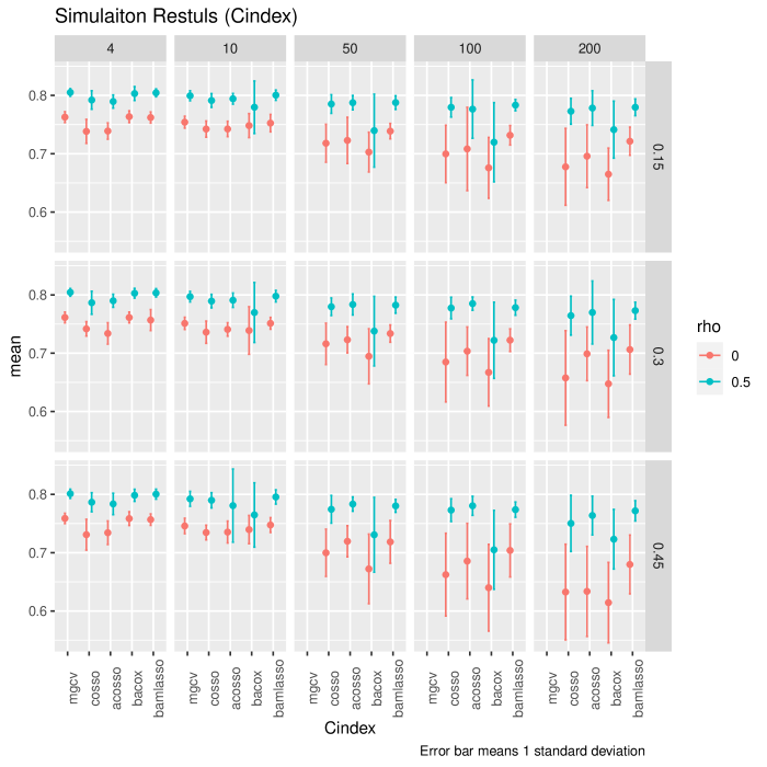
Figure 1: C-indices of out-of-sample prediction of 50 iterations of simulation studies. The models of comparison include the proposed Bayesian hierarchical additive model (BHAM), component selection and smoothing operator (COSSO), adaptive COSSO, and gcv. mgcv doesn’t provide estimation whe number of parameters exceeds sample size i.e. p = 100, 200.

Overall, we see consistent performance across different settings of dimensional, censoring rate and correlation structure (see Figure 1): the proposed bamlasso model performs as good as, if not better than previous methods, including mgcv, COSSO, adaptive COSSO. The improvement is more substantial as p increases, or higher censoring rate, or when predictors are independent. As expected, adaptive COSSO performs slightly better than COSSO.

4 Metabolites Data Analysis

In this section, we apply the proposed model BHAM to analyze a previously published metabolically dataset to study plasma metabolomic profile on the all-cause mortality among patients undergoing cardiac catheterization. The data set is publicly available via Dryad. The dataset contains data collected from two cohorts and there exists a large number of non-overlapping among metabolomic profile measured in the two cohort. Hence, we focus our analysis on the cohort that have the larger sample size (N=454). To achieve practically meaningful analysis, we select the top 200 features with largest variance from the initial 6796 features to conduct our analysis. We use 5-knot cubic splines as the additive function in the proposed Cox additive model. Optimal tuning parameters are chosen via 10-fold CV. Out-of-bag samples are used to evaluate prediction performance, where we primary focus on deviance and concordance statistics. To visualize the risk prediction, we also create two groups based on the out-of-bad risk prediction, thresholding at the median risk and labeled low-risk group and high-risk group. The Kaplan-Meier plot for the two groups is presented in Figure .

5 Discussion

In this article, we introduce the two-part spike-and-slab LASSO prior to Cox additive models for high-dimensional survival data analysis. Specifically, the proposed spike-and-slab LASSO prior adopts the sparse penalty to select effective predictors and the smooth penalty to estimate the degree of smoothness of the underlying nonlinear function. This mechanism addresses the previous criticism that high-dimensional additive models without smooth penalty tends to oversmooth the estimate of the underlying linear function. Meanwhile, the two-part prior encourages a bi-level selection of each predictor, selection of effective predictors and distinguishing linear and nonlinear effects among predictors. In addition to the Bayesian hierarchical Cox additive model proposal, we develop a optimization-based algorithm to provide a scalable solution to fit the model. This substantially reduces computational demands in comparison to posterior approximation algorithms. Lastly, we implement the proposed model and fitting algorithm in a freely available R package BHAM via https://github.com/boyiguo1/BHAM, along with many other utility functions to support model specification, tuning, and diagnostic.

Similar to many machine learning algorithms that provides flexible modeling of complex signal, the proposed model requires no assumption checking prior to the model fitting. This is because the model can automatically choose from the linear or nonlinear forms for a predictor. Such decisions are data-driven, as the underlying penalty is locally adaptive, depending on the data. Nevertheless, for the purpose of variable selection, we still encourage the authors relies on domain knowledge and consult multiple models. The proposed model can make false positive selection of linear components. For example, when the underlying model include no linear component, e.g. $x^{2}$, the proposed model still tends to include a linear effect in the model. This phenomenon is because of the effect hierarchy we impose on the prior structure. In other words, we encourage the model to include the linear component when the nonlinear effect is detected. An alternative solution, is to consider the inclusion of the linear and nonlinear effect independent. Nevertheless, this could leads to lower power to detect complex functions, i.e. including both linear and nonlinear component. Similar trade-offs of different prior construction was previously seen in [21].

In this article, we only shows the basic survival model without mentioning some other analytic problems likely to encounter in survival analysis, for example delayed entry, stratified Cox models. These analytic problems can be easily addressed and implemented under the current model framework. Another important extension of the proposed model is to model time varying effect. Such extension requires minimum modification: one can simply construct the additive function matrix for time, and multiply with the covariates. We see similar strategy was applied in [44]. In our future work, we attempt to expand the univariate additive function to multi-dimensional surface, for example via tensor product spline [5]. Hence, the interaction effect between covariates can be modeled. We also aim to extend our framework to model functional covariates following [45].

In conclusion, we proposed a new Bayesian hierarchical model to address Cox additive model in high-dimensional settings, and provide a software implementation of the proposed model. The model fitting algorithm is easily scalable and hence can benefit signal detection and risk prediction in clinical and molecular data analysis.

sim_prmt.p	sim_prmt.pi_cns	0	0.5
4	0.15	0.155 (0.021)	0.152 (0.025)
4	0.30	0.304 (0.024)	0.301 (0.029)
4	0.45	0.465 (0.033)	0.460 (0.033)
10	0.15	0.155 (0.017)	0.151 (0.025)
10	0.30	0.310 (0.027)	0.303 (0.029)
10	0.45	0.463 (0.034)	0.463 (0.032)
50	0.15	0.151 (0.022)	0.149 (0.023)
50	0.30	0.303 (0.024)	0.299 (0.030)
50	0.45	0.458 (0.033)	0.460 (0.033)
100	0.15	0.146 (0.025)	0.147 (0.023)
100	0.30	0.306 (0.031)	0.299 (0.030)
100	0.45	0.462 (0.036)	0.453 (0.030)
200	0.15	0.149 (0.023)	0.148 (0.029)
200	0.30	0.302 (0.039)	0.298 (0.036)
200	0.45	0.464 (0.034)	0.454 (0.040)

Table 1: The average and standard deviation of censoring proportion of the simulated data over 50 iterations.

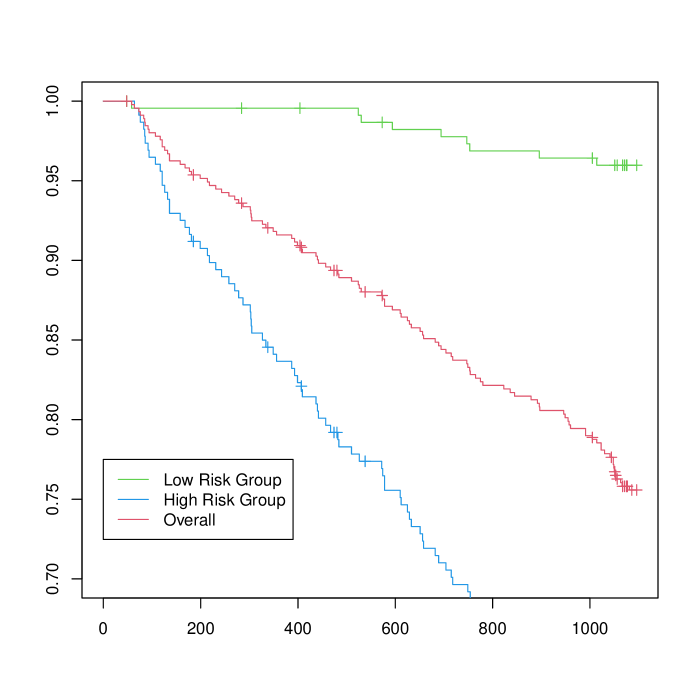
Figure 2: The Kaplan-Meier estimates to show the predictive performacne of the proposed model, including the estimates for the predicted high risk group (blue), predicted low risk group (green), and overall group (red)

References

- [1] Kyle Steenland and James A. Deddens. A practical guide to dose-response analyses and risk assessment in occupational epidemiology. Epidemiology, 15(1):63–70, 2004.
- [2] Robert J. Gray. Flexible Methods for Analyzing Survival Data Using Splines, with Applications to Breast Cancer Prognosis. Journal of the American Statistical Association, 87(420):942–951, dec 1992.
- [3] Odd Aalen. A model for nonparametric regression analysis of counting processes. In Mathematical statistics and probability theory, pages 1–25. Springer, 1980.
- [4] D. Y. Lin and Zhiliang Ying. Additive Hazards Regression Models for Survival Data, pages 185–198. Springer US, 1997.
- [5] Simon N Wood. Generalized additive models: an introduction with R. CRC press, 2017.
- [6] Ch. H. Reinsch. Smoothing by spline functions. Numerische Mathematik, 10:177–183, 1967.
- [7] ROBERT TIBSHIRANI. The lasso method for variable selection in the cox model. Statistics in Medicine, 16(4):385–395, 02 1997.
- [8] Jianqing Fan and Runze Li. Variable selection for cox’s proportional hazards model and frailty model. The Annals of Statistics, 30(1), 02 2002.
- [9] H. H. Zhang and W. Lu. Adaptive lasso for cox’s proportional hazards model. Biometrika, 94(3):691–703, 08 2007.
- [10] Yichao Wu. Elastic net for cox’s proportional hazards model with a solution path algorithm. Statistica Sinica, 22(1), 01 2012.
- [11] Jelena Bradic, Jianqing Fan, and Jiancheng Jiang. Regularization for cox’s proportional hazards model with np-dimensionality. The Annals of Statistics, 39(6), 12 2011.
- [12] Jianqing Fan, Yang Feng, and Yichao Wu. High-dimensional variable selection for Cox’s proportional hazards model, pages 70–86. Institute of Mathematical Statistics, 2010.
- [13] Pang Du, Shuangge Ma, and Hua Liang. Penalized variable selection procedure for Cox models with semiparametric relative risk. Annals of Statistics, 38(4):2092–2117, 2010.
- [14] Chenlei Leng and Hao Helen Zhang. Model selection in nonparametric hazard regression. Journal of Nonparametric Statistics, 18(7-8):417–429, 10 2006.
- [15] Heng Lian, Jianbo Li, and Yuao Hu. Shrinkage variable selection and estimation in proportional hazards models with additive structure and high dimensionality. Computational Statistics and Data Analysis, 63:99–112, 2013.
- [16] Guangren Yang, Sumin Hou, Luheng Wang, and Yanqing Sun. Feature screening in ultrahigh-dimensional additive Cox model. Journal of Statistical Computation and Simulation, 88(6):1117–1133, apr 2018.
- [17] Lukas Meier, Sara Van De Geer, and Peter Bühlmann. High-dimensional additive modeling. Annals of Statistics, 37(6 B):3779–3821, 2009.
- [18] Fabian Scheipl, Thomas Kneib, and Ludwig Fahrmeir. Penalized likelihood and bayesian function selection in regression models. AStA Advances in Statistical Analysis, 97(4):349–385, 10 2013.
- [19] Andreas Bender, Andreas Groll, and Fabian Scheipl. A generalized additive model approach to time-to-event analysis. Statistical Modelling, 18(3-4):299–321, 06 2018. Publisher: SAGE Publications India.
- [20] Jiacheng Wu and Daniela Witten. Flexible and interpretable models for survival data. Journal of computational and graphical statistics : a joint publication of American Statistical Association, Institute of Mathematical Statistics, Interface Foundation of North America, 28(4):954–966, 2019. PMID: 32704224 PMCID: PMC7377334.
- [21] Boyi Guo, Byron C. Jaeger, A. K. M. Fazlur Rahman, D. Leann Long, and Nengjun Yi. Spike-and-slab lasso generalized additive models and scalable algorithms for high-dimensional data analysis. arXiv:2110.14449 [stat], 04 2022. arXiv: 2110.14449.
- [22] R Core Team. R: A Language and Environment for Statistical Computing. R Foundation for Statistical Computing, Vienna, Austria, 2021.
- [23] John P. Klein and Melvin L. Moeschberger. Survival Analysis. Statistics for Biology and Health. Springer New York, New York, NY, 2003.
- [24] Joseph G. Ibrahim, Ming Hui Chen, and Debajyoti Sinha. Bayesian semiparametric models for survival data with a cure fraction. Biometrics, 2001.
- [25] D. R. Cox. Regression models and life-tables. Journal of the Royal Statistical Society: Series B (Methodological), 34(2):187–202, 1972. _eprint: https://onlinelibrary.wiley.com/doi/pdf/10.1111/j.2517-6161.1972.tb00899.x.
- [26] Bradley Efron. The efficiency of cox’s likelihood function for censored data. Journal of the American Statistical Association, 1977.
- [27] N. Breslow. Covariance analysis of censored survival data. Biometrics, 30(1):89, 03 1974.
- [28] Giampiero Marra and Simon N Wood. Practical variable selection for generalized additive models. Computational Statistics & Data Analysis, 55(7):2372–2387, 2011.
- [29] Zaixiang Tang, Shufeng Lei, Xinyan Zhang, Zixuan Yi, Boyi Guo, Jake Y. Chen, Yueping Shen, and Nengjun Yi. Gsslasso cox: a bayesian hierarchical model for predicting survival and detecting associated genes by incorporating pathway information. BMC Bioinformatics, 20(1):94, 12 2019.
- [30] Veronika Ročková. Bayesian estimation of sparse signals with a continuous spike-and-slab prior. The Annals of Statistics, 46(1):401–437, 02 2018. Publisher: Institute of Mathematical Statistics.
- [31] Veronika Ročková and Edward I. George. The spike-and-slab lasso. Journal of the American Statistical Association, 113(521):431–444, 01 2018.
- [32] Zaixiang Tang, Yueping Shen, Yan Li, Xinyan Zhang, Jia Wen, Chen’ao Qian, Wenzhuo Zhuang, Xinghua Shi, and Nengjun Yi. Group spike-and-slab lasso generalized linear models for disease prediction and associated genes detection by incorporating pathway information. Bioinformatics, 34(6):901–910, 03 2018.
- [33] Hugh Chipman. Prior distributions for bayesian analysis of screening experiments. In Screening, pages 236–267. Springer, 2006.
- [34] Ray Bai. Spike-and-slab group lasso for consistent estimation and variable selection in non-gaussian generalized additive models. arXiv:2007.07021 [stat], 06 2021. arXiv: 2007.07021.
- [35] Veronika Ročková and Edward I. George. Emvs: The em approach to bayesian variable selection. Journal of the American Statistical Association, 109(506):828–846, 04 2014.
- [36] Zaixiang Tang, Yueping Shen, Xinyan Zhang, and Nengjun Yi. The spike-and-slab lasso cox model for survival prediction and associated genes detection. Bioinformatics, 33(18):2799–2807, 05 2017.
- [37] Debajyoti Sinha, Joseph G Ibrahim, and Ming-Hui Chen. A bayesian justification of cox’s partial likelihood. Biometrika, 90(3):629–641, 09 2003.
- [38] Noah Simon, Jerome Friedman, Trevor Hastie, and Rob Tibshirani. Regularization paths for cox’s proportional hazards model via coordinate descent. Journal of Statistical Software, 39(5), 2011.
- [39] Curtis B. Storlie, Howard D. Bondell, Brian J. Reich, and Hao Helen Zhang. Surface estimation, variable selection, and the nonparametric oracle property. Statistica Sinica, 21(2):679, 04 2011.
- [40] Hao Helen Zhang and Chen-Yen Lin. cosso: Fit Regularized Nonparametric Regression Models Using COSSO Penalty, 2013. R package version 2.1-1.
- [41] Simon Wood. mgcv: Mixed GAM Computation Vehicle with Automatic Smoothness Estimation, 2022. R package version 1.8-31.
- [42] Samuel L. Brilleman, Rory Wolfe, Margarita Moreno-Betancur, and Michael J. Crowther. Simulating survival data using the simsurv R package. Journal of Statistical Software, 97(3):1–27, 2020.
- [43] Fei Wan. Simulating survival data with predefined censoring rates for proportional hazards models. Statistics in Medicine, 36(5):838–854, 11 2016.
- [44] Lifeng Wang, Guang Chen, and Hongzhe Li. Group scad regression analysis for microarray time course gene expression data. Bioinformatics, 23(12):1486–1494, 06 2007.
- [45] Erjia Cui, Ciprian M. Crainiceanu, and Andrew Leroux. Additive functional cox model. Journal of Computational and Graphical Statistics, 30(3):780–793, 01 2021.