Analysis and sample size calculation within the responder stratified exponential survival model

Abstract

The primary endpoint in oncology is usually overall survival, where differences between therapies may only be observable after many years. To avoid withholding of a promising therapy, preliminary approval based on a surrogate endpoint is possible. The approval can be confirmed later by assessing overall survival within the same study. In these trials, the correlation between surrogate endpoint and overall survival has to be taken into account for sample size calculation and analysis. For a binary surrogate endpoint, this relation can be modeled by means of the responder stratified exponential survival (RSES) model proposed by Xia, Cui, and Yang (2014). We derive properties of the model and confidence intervals based on Maximum Likelihood estimators. Furthermore, we present an approximate and an exact test for survival difference. Type I error rate, power, and required sample size for both newly developed tests are determined exactly. These characteristics are compared to those of the logrank test. We show that the exact test performs best. The power of the logrank test is considerably lower in some situations. We conclude that the logrank test should not be used within the RSES model. The proposed method for sample size calculation works well. The interpretability of our proposed methods is discussed.

Keywords accelerated approval  $\cdot$ stratification  $\cdot$ survival  $\cdot$ exact tests

1 Introduction

Endpoints of clinical trials should be appropriate for answering the research question, objectively measurable, and relevant for patients. Thus, for proving efficacy of a new oncological therapy, the primary endpoint is usually overall survival. The new therapy is compared to the present gold standard. However, as therapies get better and diagnoses are made in earlier stages, differences between therapies may only be observable after many years. This may considerably delay approval of new treatments and their application in practice.

To avoid withholding of a promising therapy, the Food and Drug Administration (FDA) provides four different programs for expedited development of new therapies (Wallach, Ross, and Naci 2018). One of them is the Accelerated Approval pathway, where the approval is based on a surrogate endpoint. The approval is preliminary and has to be confirmed later when the main endpoint can be assessed. Between 1992 and 2021, 278 preliminary accelerated approvals were granted by the FDA after a median processing time of 6 months. Of these, 50% were confirmed later, 10% were withdrawn, and 40% are still ongoing (Food and Drug Administration 2022).

In 2014, the FDA published a more detailed guidance (which was updated in 2020) regarding the use of pathological complete response (pCR) as a surrogate endpoint when approving a novel neoadjuvant treatment of high-risk early-stage breast cancer (Food and Drug Administration 2020). Although the appropriateness of pCR as surrogate endpoint is disputed (Conforti et al. 2021), the guidance illustrates the use of a binary surrogate endpoint for survival. When accelerated and final approval are sought within the same study, the correlation between surrogate endpoint and survival has to be taken into account for sample size calculation and analysis. The relationship can be modeled by means of a conditional survival proposed by Xia, Cui, and Yang (2014). They investigated the correlation and assessed the power of the logrank test. Howevver, they did not present methods for statistical testing, parameter estimation, and sample size calculation. This gap constitutes a major hurdle for the application of this approach.

The aim of our work is to develop methods for analysis and sample size calculation within the conditional survival model by Xia, Cui, and Yang (2014). In this article, we focus on the analysis of the survival endpoint that is assessed at the end of the trial. Due to the non-proportionality of the hazards within the model, standard methods like the logrank test may not be the most powerful. The analysis of the surrogate endpoint is built into the proposed testing strategy with global Type I error control. However, the proposed sample size calculation method is tailored to the final survival endpoint and does not consider possible interim decisions after assessment of the surrogate endpoint.

In Section 2, we define the model and explain the possible constellations of marginal survival functions in a two-group model. We derive Maximum Likelihood estimators and approximate confidence intervals for the parameters in the third section. Based on that, an approximate and an exact hypothesis test are derived in Section 4. Type I error and power of these tests are evaluated in the fifth section. An approximate sample size calculation method is derived and evaluated in the sixth section. Furthermore, exact sample size calculation is outlined. Finally, approximate sample sizes and exact power values are calculated and compared for parameter values derived from clinical trial data. The manuscript concludes with a discussion, while technical details are given in the appendices.

2 Statistical model

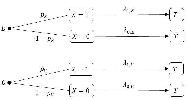
The responder stratified exponential survival (RSES) model was proposed by Xia, Cui, and Yang (2014). They did not specifically name their model back then, we, however, decided to denote it as the RSES model throughout the course of this manuscript. It models the survival time of a patient as an exponentially distributed random variable with the parameter depending on the response status of the patient. Formally, the random variable $X$ distinguishes the responders ($X=1$) from the non-responders ($X=0$) and is Bernoulli distributed with probability $p$. The survival time $T|X=1$ of a responder follows a $\mathrm{Exp}(\lambda_{1})$-distribution and the survival time $T|X=0$ of a non-responder follows a $\mathrm{Exp}(\lambda_{0})$-distribution. Figure 1 visualizes the model in two treatment groups. The common distribution function of the random vector $(X,T)$ is

$$F_{p,\lambda_{1},\lambda_{0}}(x,t)=x\cdot p\cdot\left(1-\exp(-\lambda_{1}t)\right)+(1-x)\cdot(1-p)\cdot\left(1-\exp(-\lambda_{0}t)\right).$$

The common density function is

$$f_{p,\lambda_{1},\lambda_{0}}(x,t)=x\cdot p\cdot\lambda_{1}\exp(-\lambda_{1}t)+(1-x)\cdot(1-p)\cdot\lambda_{0}\exp(-\lambda_{0}t).$$

Figure 1: Two-group RSES model. Experimental (E) and control (C) group are each defined by a set of three parameters.

By integrating over $x$, we get the marginalized distribution of the survival time:

$$\tilde{F}_{p,\lambda_{1},\lambda_{0}}(t)=p\cdot\left(1-\exp(-\lambda_{1}t)\right)+(1-p)\cdot\left(1-\exp(-\lambda_{0}t)\right)$$

Thus, the survival function is

$$S_{p,\lambda_{1},\lambda_{0}}(t) =1-\tilde{F}_{p,\lambda_{1},\lambda_{0}}(t)$$

$$=p\cdot\exp(-\lambda_{1}t)+(1-p)\cdot\exp(-\lambda_{0}t).$$

When comparing the experimental group $E$ with the control group $C$, differences within the three-parameter model may not be easily interpretable. Specifically, a difference in parameter sets does not imply a global survival benefit of one group neither does it imply a survival difference between groups.

Let $p_{i},\lambda_{1,i},\lambda_{0,i}$ be the respective parameter sets of the groups as shown in Figure 1. For better readability, $S_{p_{i},\lambda_{1,i},\lambda_{0,i}}$ will be abbreviated as $S_{i}$. We can distinguish three cases of the relation of $S_{E}$ and $S_{C}$:

1. Completely equal: $S_{E}(t)=S_{C}(t)\quad\forall t\geq 0$

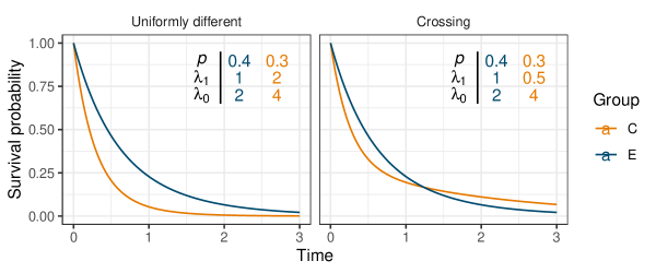
2. Uniformly different: $S_{E}(t)\neq S_{C}(t)\quad\forall t>0$

3. Crossing: not completely equal but $\exists\ t>0$ such that $S_{E}(t)=S_{C}(t)$

See Appendix A.1 for a detailed analysis of these cases.

Figure 2 shows two examples. In the first, the experimental group has a higher response probability and better survival of each responders and non-responders. Thus, survival in the experimental group is uniformly better. In the second example, responder survival is better in the control group. This advantage comes into effect after a certain time which leads to crossing survival curves.

Figure 2: Survival functions of two different two-group models.

3 Maximum Likelihood estimation

In this section, estimators of the model parameters are derived by the Maximum Likelihood method. Suppose we observe $n$ realisations $(x_{i},t_{i})$ of response status and survival time. For simplicity, we assume that there is no censoring. The inclusion of censoring will be addressed in the Discussion. Let $k=\sum_{i=1}^{n}x_{i}$ be the number of responders. We arrange our observations such that $x_{1}=\dots=x_{k}=1$ and $x_{k+1}=\dots=x_{n}=0$. Denote $\theta_{i}=\log(\lambda_{i})$. Then the Maximum Likelihood estimates of the parameters $p,\theta_{1}$ and $\theta_{0}$ are

$$\hat{p} =\frac{k}{n},$$

$$\hat{\theta}_{1} =-\log\left(\frac{1}{k}\sum\limits_{i=1}^{k}t_{i}\right),$$

$$\hat{\theta}_{0} =-\log\left(\frac{1}{n-k}\sum\limits_{i=k+1}^{n}t_{i}\right).$$

See Appendix A.2 for a detailed derivation of the MLEs and their asymptotic covariance structure. Note that the estimation of $\hat{\theta}_{1}$ is only well-defined if $k\neq 0$. In the case $k=0$ there is no unique Maximum Likelihood estimator for $\theta_{1}$. The same holds for $\theta_{0}$ if $k=n$.

The asymptotic distribution of the MLE is multivariate normal with the true parameter vector as mean and the inverse Fisher information matrix as covariance matrix.
This yields

$$\mathrm{Var}(\hat{p}) \approx\frac{p\cdot(1-p)}{n},$$

$$\mathrm{Var}(\hat{\theta}_{1}) \approx\frac{1}{np},$$

$$\mathrm{Var}(\hat{\theta}_{0}) \approx\frac{1}{n(1-p)},$$

$$\mathrm{Cov}(\hat{p},\hat{\theta}_{i}) \approx 0,$$

$$\mbox{and }\mathrm{Cov}(\hat{\theta}_{1},\hat{\theta}_{0}) \approx 0.$$

In particular, the MLEs of the different parameters are asymptotically uncorrelated.

Also, the exact distribution of the MLEs can be given explicitly: $n\cdot\hat{p}=k$ follows a binomial distribution with parameters $n$ and $p$. Conditional on $k$, $\sum\limits_{i=1}^{k}t_{i}$ follows a $\Gamma(k,\lambda_{1})$-distribution and thus

$$\exp(-\hat{\theta}_{1})\sim\Gamma(k,k\lambda_{1}).$$

Asymptotic confidence intervals for the parameters can be constructed by using the asymptotic normality of the MLEs. For $p$ this yields the well known normal approximation confidence interval

$$\mathrm{CI}_{p}(\hat{p})=\hat{p}\pm z_{1-\alpha/2}\cdot\sqrt{\hat{p}(1-\hat{p})/n}.$$

For $\theta_{1}$ we obtain

$$\mathrm{CI}_{\theta_{1}}(\hat{\theta}_{1},\hat{p})=\hat{\theta}_{1}\pm z_{1-\alpha/2}\cdot\sqrt{1/(n\hat{p})},$$

and for $\theta_{0}$

$$\mathrm{CI}_{\theta_{0}}(\hat{\theta}_{0},\hat{p})=\hat{\theta}_{0}\pm z_{1-\alpha/2}\cdot\sqrt{1/\left(n(1-\hat{p})\right)}.$$

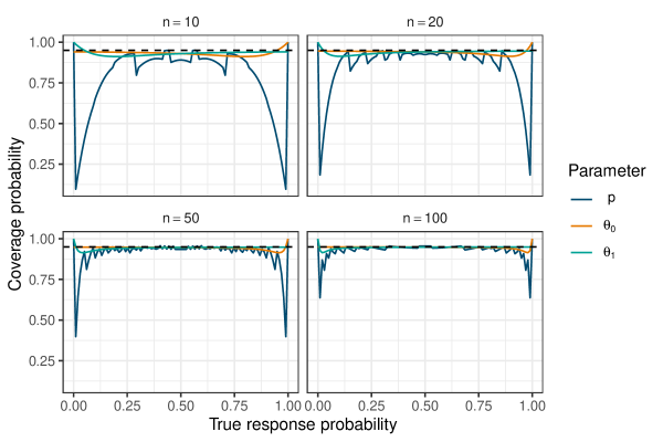
If $\hat{p}=0$ (or $\hat{p}=1$), the confidence interval for $\theta_{1}$ (or $\theta_{0}$) cannot be computed and is formally set to $(-\infty,\infty)$ to enable calculation of coverage probabilities. See Appendix A.3 for details of the calculation. Figure 3 shows the coverage probability of the asymptotic 95% confidence intervals for different sample sizes and true response probabilites. The coverage probability of $\mathrm{CI}_{\theta_{1}}$ and $\mathrm{CI}_{\theta_{0}}$ is pretty good overall. The coverage probability of $\mathrm{CI}_{p}$ is generally lower and much too low for extreme probabilites and small sample sizes.

Figure 3: Exact coverage probability of approximate confidence intervals for various values of $p$ and sample sizes.

4 Hypothesis testing

There are different ways to formulate a null hypothesis regarding the RSES model. In this article, we are testing the difference of parameter sets. We consider the comparison of an experimental group $E$ and a control group $C$ with respective parameter triples $(p_{E},\theta_{1,E},\theta_{0,E})$ and $(p_{C},\theta_{1,C},\theta_{0,C})$. We want to test the null hypothesis

$$H_{0}:p_{C}=p_{E},\theta_{1,C}=\theta_{1,E}\mbox{ and }\theta_{0,C}=\theta_{0,E}.$$

Note that this is not a neccessary condition for equality of the marginal survival distributions as we saw in Section 2. This procedure aims at detecting any group difference within the parametric model. In particular, it is not meant to make inference about differences of single parameters because they can only be interpreted and translated to survival difference when considered as a triple.

Our global null hypothesis $H_{0}$ is an intersection of three local null hypotheses:

$$H_{p,0}\mbox{: } p_{C}=p_{E}$$

$$H_{\theta_{1},0}\mbox{: } \theta_{1,C}=\theta_{1,E}$$

$$H_{\theta_{0},0}\mbox{: } \theta_{0,C}=\theta_{0,E}$$

Firstly, we will construct asymptotic Wald-like tests for the local test problems. By splitting the desired significance level $\alpha$ into local levels $\tilde{\alpha}$, this will give an asymptotic test for the global null hypothesis. Secondly, we will construct an exact test based on the exact distribution of the test statistics.

4.1 Approximate test

We construct test statistics for the local hypotheses by standardizing the difference between the MLEs of both groups. It is divided by the standard deviation of the difference. Here, the unknown true response probabilities are replaced by their MLEs under the null hypothesis. The MLE of the response probability under $H_{0}$ is $\hat{p}=\frac{n_{E}\hat{p}_{E}+n_{C}\hat{p}_{C}}{n_{E}+n_{C}}$.

For the test of $H_{p,0}$, this yields the well-known two-sample binomial $z$-test with test statistic

$$T_{p}=\frac{\hat{p}_{E}-\hat{p}_{C}}{\sqrt{\hat{p}(1-\hat{p})(\frac{1}{n_{E}}+\frac{1}{n_{C}})}}.$$

If $\hat{p}\in\{0,1\}$ (which means that everyone or no one is a responder), we set $T_{p}=0$ because we would not reject $H_{p,0}$ in this case.

The test statistic for the local test of $H_{\theta_{1},0}$ is

$$T_{\theta_{1}}=\frac{\hat{\theta}_{1,E}-\hat{\theta}_{1,C}}{\sqrt{\frac{1}{\hat{p}}(\frac{1}{n_{E}}+\frac{1}{n_{C}})}}.$$

If the number of responders $k_{E},k_{C}$ in one of the groups equals zero, we set $T_{\theta_{1}}=0$ because we cannot make a statement about survival of responders in one of the groups and thus would not reject $H_{\theta_{1},0}$.

Analogously, the test statistic for the local test of $H_{\theta_{0},0}$ is

$$T_{\theta_{0}}=\frac{\hat{\theta}_{0,E}-\hat{\theta}_{0,C}}{\sqrt{\frac{1}{(1-\hat{p})}(\frac{1}{n_{E}}+\frac{1}{n_{C}})}}.$$

Again, if $k_{E}=n_{E}$ or $k_{C}=n_{C}$, we set $T_{\theta_{0}}=0$ because we cannot make a statement about survival of non-responders in one of the groups and thus would not reject $H_{\theta_{0},0}$.

The three test statistics are asymptotically standard normally distributed under their respective null hypothesis. Since the MLEs are asymptotically uncorrelated, the three test statistics are also asymptotically uncorrelated. Thus, we test the intersection of the three local hypotheses by assuming independence of the test statistics and testing every hypothesis at level $\tilde{\alpha}=1-\sqrt[3]{1-\alpha}$. The global hypothesis $H_{0}$ can be rejected if at least one of the local hypotheses can be rejected. This will asymptotically control the Type I error rate at the level $\alpha$. The level $\tilde{\alpha}$ is based on an equal split of $\alpha$. However, the procedure can easily be adapted to other allocation methods.

4.2 Exact test

To construct an exact test, we test $H_{\theta_{1},0}$ and $H_{\theta_{0},0}$ conditionally on $k_{E}$ and $k_{C}$. By doing so, the test statistic $T_{\theta_{1}}$ becomes a monotone transformation of the simplified test statistic

$$\tilde{T}_{\theta_{1}}:=\frac{k_{C}\bar{T}_{1,C}}{k_{E}\bar{T}_{1,E}}.$$

$\frac{\lambda_{1,C}}{\lambda_{1,E}}\tilde{T}_{\theta_{1}}$ follows a beta prime distribution:

$$\frac{\lambda_{1,C}}{\lambda_{1,E}}\tilde{T}_{\theta_{1}}\sim\beta^{\prime}(k_{C},k_{E}).$$

This distribution is also known as beta distribution of the second kind (Johnson, Kotz, and Balakrishnan 1995) and can be defined by its density

$$f_{\alpha,\beta}(x)=\frac{x^{\alpha-1}(1+x)^{-\alpha-\beta}}{B(\alpha,\beta)}\quad\quad\mbox{for }x>0,$$

where $B$ is the Beta function. Thus, under the null hypothesis $\lambda_{1,E}=\lambda_{1,C}$, the exact distribution of $\tilde{T}_{\theta_{1}}$ is independent of $\lambda_{1,E},\lambda_{1,C}$. The same can be done for $\tilde{T}_{\theta_{0}}$.

$H_{p,0}$ can be tested exactly by using any exact test for the comparison of two binomial proportions, e.g. Boschloo’s test (Boschloo 1970). For consistency, we use an exact test based on the test statistic $T_{p}$, which Mehrotra, Chan, and Berger (2003) named Z-Pooled Exact Unconditional Test.

Hence, the exact test procedure consists in computing the exact local p-value $p_{p}$ for the test of $H_{p,0}$ and the exact local p-values $p_{\theta_{1}}$ and $p_{\theta_{0}}$ conditionally on $k_{E}$ and $k_{C}$. If one of the p-values is smaller than the local level $\tilde{\alpha}$, we reject the global hypothesis $H_{0}$. This procedure yields an exact test for $H_{0}$ controlling the Type I error rate at the level $\alpha$ (see Appendix A.4).

5 Assessment of test characteristics and comparison to logrank test

In this section, we analyse Type I error rate and power of the approximate and the exact test and compare it to the logrank test and the stratified logrank test. See Appendix A.5 for details of the used logrank test statistics. Note that stratifying the logrank test for response status deliberately ignores a survival benefit originating from a response benefit. Thus, the stratified logrank test is not appropriate in our setting. However, we included it for comparison purposes because Xia, Cui, and Yang (2014) considered it as well.

Rejection probabilities for the proposed tests were calculated exactly. For the logrank tests, rejection probabilities were estimated by simulation with $10^{5}$ runs per scenario, resulting in a standard error of 0.0007 for the Type I error and a maximal standard error of 0.0016 for the power.

5.1 Assessment of Type I error rate

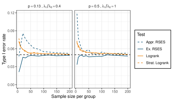
We evaluated the Type I error rate in various scenarios and found similar results in all of them. Thus, we chose two representative scenarios for illustration. In the first setting, survival of responders and non-responders is equal and the response probability equals 0.5 in both groups. In the second scenario, survival of responders is better, with a hazard ratio of 0.4, and the response probability equals 0.13 in both groups. No difference with regard to survival is assumed between experimental and control group. Figure 4 shows Type I error rates for sample sizes per group from 5 to 200. The exact test always adheres to the nominal level and exploits it even for small sample sizes. The two logrank tests and the approximate RSES test exceed the nominal level for small sample sizes but the two logrank tests converge faster to the desired value. The approximate test performs worse for smaller response probabilities. This is due to the fact that the normal approximation of $T_{p}$ is worse. Furthermore, the expected size of the responder stratum is smaller and thus the normal approximation of $T_{\theta_{1}}$ is worse. The same holds true for response probabilities near 1.

Interestingly, Type I error rate of the asymptotic test is lower for very small sample sizes and response probabilities. This is because in these cases it is likely that one of the groups does not include any responders, which prevents rejection of $H_{\theta_{1},0}$. The same holds true for response probabilities near 1.

Figure 4: Type I error rate for various sample sizes in different scenarios.

5.2 Assessment of Power

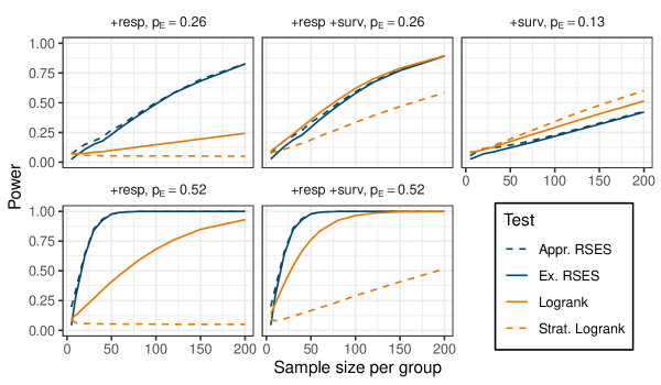
We consider five different scenarios for the evaluation of the power. In all scenarios, responder survival is better than non-responder survival with a hazard ratio of $\lambda_{1}/\lambda_{0}=0.4$. In the first two scenarios (+resp), survival benefit of the experimental group is solely due to a higher response probability ($p_{E}=0.26,0.52$ vs. $p_{C}=0.13$). In Scenarios 3 and 4 (+resp +surv), there is additionally a survival benefit of the experimental group within the strata. That means that responders in the experimental group have a better survival than responders in the control group and non-responders in the experimental group have a better survival than non-responders in the control group. In Scenario 5 (+surv), the response probabilities are equal in both groups. The survival benefit of the experimental group is solely due to a better survival of both responders and non-responders.

Figure 5 shows power for sample sizes per group from 5 to 200. In all scenarios, the approximate RSES test has slightly greater power than the exact test. However, the difference is not meaningful.

When survival benefit is solely due to response benefit (+resp), the RSES tests are much more powerful than the logrank test. Since the stratified logrank test only considers survival differences within the response strata, its power equals the significance level.

The higher the survival benefit within the strata compared to the response benefit, the better perform the logrank tests compared to the RSES tests. This is because they don’t spend significance level to test response difference. When there is no response difference at all (+surv), the logrank tests are more powerful.

Interestingly, power of the stratified logrank test is not always monotonically increasing for very small sample sizes. This is because in these cases it is likely that one of the strata is empty. Then the stratified logrank test becomes a usual logrank test restricted to the non-empty stratum and can be more powerful than a stratified logrank test on two slightly bigger strata.

Figure 5: Power with respect to sample size in different treatment effect scenarios.

6 Sample size calculation

Since both the approximate and the exact RSES test are based on the same test statistics with the same asymptotic distributions, approximate sample size calculation is valid for both tests. Exact sample size calculation differs for both tests and is only presented for the exact test.

6.1 Approximate sample size calculation

Firstly, we derive for the three local tests approximate formulas for the probabilities to falsely accept the respective null hypothesis. This can be done using the asymptotic normality of the test statistics. Let $n_{E},n_{C}$ be the sample sizes and $p_{i}^{\prime},\theta_{j,i}^{\prime}$ the specified parameter values under the assumed alternative hypothesis for $i=E,C,j=0,1$. Then the approximate probabilities for falsely accepting the respective null hypothesis of the three local tests are

$$\beta_{p} =\Phi\left(\frac{z_{1-\frac{\tilde{\alpha}}{2}}\cdot\sqrt{\tilde{p}(1-\tilde{p})(\frac{1}{n_{E}}+\frac{1}{n_{C}})}-(p_{E}^{\prime}-p_{C}^{\prime})}{\sigma_{p}^{\prime}}\right),$$

$$\beta_{\theta_{1}} =\Phi\left(\frac{z_{1-\tfrac{\alpha}{2}}\cdot\sqrt{\tfrac{1}{\tilde{p}}\cdot(\tfrac{1}{n_{E}}+\tfrac{1}{n_{C}})}-(\theta_{1,C}^{\prime}-\theta_{1,E}^{\prime})}{\sigma_{\theta_{1}}^{\prime}}\right),$$

$$\beta_{\theta_{0}} =\Phi\left(\frac{z_{1-\tfrac{\alpha}{2}}\cdot\sqrt{\tfrac{1}{(1-\tilde{p})}\cdot(\tfrac{1}{n_{E}}+\tfrac{1}{n_{C}})}-(\theta_{0,C}^{\prime}-\theta_{0,E}^{\prime})}{\sigma_{\theta_{0}}^{\prime}}\right),$$

with

$$\tilde{p}:=\frac{n_{E}p_{E}^{\prime}+n_{C}p_{C}^{\prime}}{n_{E}+n_{C}}.$$

See Appendix A.6 for the derivation of the formulas. Due to the asymptotic independence of the three test statistics, the probability to not reject $H_{0}$, i.e. to accept all three local null hypotheses simultaneously, is approximately equal to the product of the acceptance probabilities of the three local null hypotheses.

Let $r=n_{E}/n_{C}$ be the desired sample size ratio. We specify power $1-\beta$, significance level $\alpha$, and all distribution parameters, and set the local level to $\tilde{\alpha}=1-\sqrt[3]{1-\alpha}$. Then, due to ${n_{E}=r\cdot n_{C}}$, the acceptance probabilities of the three local tests can be viewed as functions of $n_{C}$. Thus, the required control group sample size $n_{C}$ is the solution of the equation

$$\beta_{p}(n_{C})\cdot\beta_{\theta_{1}}(n_{C})\cdot\beta_{\theta_{0}}(n_{C})=\beta,$$

which can be determined numerically.

This approach also leaves the possibility of splitting Type I or Type II error rate differently to weight certain hypotheses. The calculation method can easily be adapted to such changes.

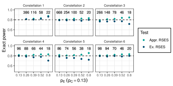
Figure 6 shows the exact power of exact and approximate test using the approximate sample size calculation in 29 different scenarios. We set the non-responder hazard to ${\gamma:=0.142}$ and the sample size ratio to $r=1$. We consider the following six constellations of responder and non-responder survival:

1. Equal survival in all strata: $\lambda_{0,E}=\lambda_{0,C}=\lambda_{1,E}=\lambda_{1,C}=\gamma$

2. Better survival of responders in experimental group (1): $\lambda_{0,C}=\lambda_{0,E}=\lambda_{1,C}=\gamma$ and $\lambda_{1,E}=\gamma/2$

3. Better survival of responders in experimental group (2): $\lambda_{0,C}=\lambda_{0,E}=\lambda_{1,C}=\gamma$ and $\lambda_{1,E}=\gamma/3$

4. Better survival of responders and non-responders in experimental group: $\lambda_{0,C}=\lambda_{1,C}=\gamma$ and $\lambda_{0,E}=\lambda_{1,E}=\gamma/2$

5. Better survival of non-responders in experimental group, even better survival of responders in experimental group: $\lambda_{0,C}=\lambda_{1,C}=\gamma,\lambda_{0,E}=\gamma/2$ and $\lambda_{1,E}=\gamma/3$

6. Better survival of responders in control group, better survival of non-responders in experimental group, even better survival of responders in experimental group: $\lambda_{0,C}=\gamma,\lambda_{1,C}=\gamma/2,\lambda_{0,E}=\gamma/2$ and $\lambda_{1,E}=\gamma/3$

In each of these constellations, response probability in the control group is $p_{C}=0.13$. We consider five different response probabilities in the experimental group: ${p_{E}=0.13,\ 0.26,\ 0.39,\ 0.52,\ 0.8}$. When response probabilities are equal in the first constellation, there is no group difference. Hence, no sample size can be calculated in this case.

We see that the approximate sample size calculation method works pretty well for the approximate test and slightly underestimates the required sample size for the exact test in most scenarios. This is consistent with the small power advantage of the approximate test seen in Section 5.2. If the response probabilities and responder and non-responder survival differ strongly between the two groups, the power drops considerably below the desired value. This correlates with an increased Type I error rate of the approximate test in such cases.

Figure 6: Exact power of approximate sample sizes in various scenarios. Calculated sample sizes are shown in the top row.

6.2 Exact sample size calculation

Exact sample size calculation can be done iteratively because power can be calculated exactly. The power of the exact RSES test of a specific alternative $H_{A}$ with parameters $p_{i,A},\theta_{1,i,A},\theta_{0,i,A}$ (${i=E,C}$) is given by

$$P_{H_{A}}(\mathrm{Rej.}H_{0}) =P_{p_{E,A},p_{C,A}}(\mathrm{Rej.}H_{p,0})$$

$$\quad+\sum_{(k_{E},k_{C})\notin R_{p}}f_{p_{E,A},p_{C,A}}(k_{E},k_{C})\cdot\left(1-u_{1}(k_{E},k_{C})\cdot u_{0}(n_{E}-k_{E},n_{C}-k_{C})\right).$$

Here, $R_{p}$ is the rejection region of the exact test of $H_{p,0}$. Furthermore, $u_{1}(k_{E},k_{C})=u_{\lambda_{1,E,A},\lambda_{1,C,A}}(k_{E},k_{C})$ is the probability to not reject $H_{\theta_{1},0}$ if the true parameters are $\lambda_{1,E,A},\lambda_{1,C,A}$ and the group sizes are $k_{E},k_{C}$. If $k_{E}=0$ or $k_{C}=0$, we have $u_{\lambda_{E,A},\lambda_{C,A}}(k_{E},k_{C})=1$ (“empty group cases”). In all other cases we have

$$u_{\lambda_{E,A},\lambda_{C,A}}(k_{E},k_{C})$$

$$=P_{\lambda_{E,A},\lambda_{C,A}}\left(-c_{\lambda}(k_{E},k_{C},\tilde{\alpha})\leq\tilde{T}_{\theta_{1}}\leq c_{\lambda}(k_{E},k_{C},\tilde{\alpha})\right)$$

$$=P\left(\frac{\lambda_{1,C}k_{C}}{\lambda_{1,E}k_{E}}\cdot\exp\left(-c_{\lambda}(k_{E},k_{C},\tilde{\alpha})\right)\leq\frac{\lambda_{1,C}k_{C}}{\lambda_{1,E}k_{E}}\cdot\exp(\tilde{T}_{\theta_{1}})\leq\frac{\lambda_{1,C}k_{C}}{\lambda_{1,E}k_{E}}\cdot\exp\left(c_{\lambda}(k_{E},k_{C},\tilde{\alpha})\right)\right)$$

$$=F_{\beta^{\prime}(k_{C},k_{E})}\left(\frac{\lambda_{1,C}k_{C}}{\lambda_{1,E}k_{E}}\cdot\exp\left(c_{\lambda}(k_{E},k_{C},\tilde{\alpha})\right)\right)-F_{\beta^{\prime}(k_{C},k_{E})}\left(\frac{\lambda_{1,C}k_{C}}{\lambda_{1,E}k_{E}}\cdot\exp\left(-c_{\lambda}(k_{E},k_{C},\tilde{\alpha})\right)\right).$$

$c_{\lambda}(k_{E},k_{C},\tilde{\alpha})$ is the critical value of the two-sided test of $H_{\theta_{1},0}$ conditionally on the numbers of responders $k_{E},k_{C}$. It is defined by the equation

$$1-F_{\beta^{\prime}(k_{C},k_{E})}\left(k_{C}/k_{E}\cdot\exp\left(c_{\lambda}(k_{E},k_{C},\tilde{\alpha})\right)\right)+F_{\beta^{\prime}(k_{C},k_{E})}\left(k_{C}/k_{E}\cdot\exp\left(-c_{\lambda}(k_{E},k_{C},\tilde{\alpha})\right)\right)=\tilde{\alpha}$$

and can be calculated numerically.

Analogously, $u_{0}(n_{E}-k_{E},n_{C}-k_{C})=u_{\lambda_{0,E,A},\lambda_{0,C,A}}(n_{E}-k_{E},n_{C}-k_{C})$ is the probability to not reject $H_{\theta_{0},0}$. Thus, the exact sample size can be calculated iteratively as follows:

1. Start with the approximate sample size.

2. Calculate exact power $P_{H_{A}}(\mathrm{Rej.}H_{0})$.

3. Increase sample size if power is too low, decrease sample size if power is too high.

4. Iterate steps 2 and 3.

7 Example

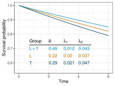
Huober et al. (2019) investigated the effect of Lapatinib (L), Trastuzumab (T), and a combination of both on pathologic complete response and survival in patients with HER2-positive early breast cancer. They reported group-wise response rates, and event-free as well as overall survival rates. Furthermore, they estimated hazard ratios between responders and non-responders within the treatment groups. Under the assumption of exponentially distributed survival within the response strata, the RSES distribution parameters can be derived. For overall survival, they are given in Figure 7 together with the survival functions. Under these assumptions, survival of responders is considerably better in all groups. Due to the highest response probability and the best survival for responders, the combination L+T has the best overall survival. Even though a treatment with T leads to a higher repsonse probability compared to L, the non-responder survival in T is worse and the responder survival is almost equal. This results in a better survival of L compared to T.

Table 1 shows approximate sample sizes per group for the three pairwise comparisons between the three groups at global level 0.05 and global power 0.8. They are calculated for the exact test by the method described in Section 6. Furthermore, exact power values for the exact test and simulation-based power values for the logrank test and stratified logrank test are given. Compared to T, L+T has a response advantage and a survival advantage in both strata and the logrank test is more powerful than the exact test. In the other two comparisons, the differences between response probability and stratified survival are not uniform and partly compensate each other when compared by the logrank test. Thus, the logrank test has lower power than the exact test. Since the stratified logrank test deliberately ignores any survival benefit arising from a response benefit, it has low power for the comparison L+T vs. T, although the survival curves show the greatest difference. The power of the stratified logrank test for the comparison between L + T and T is even lower due to the fact that it is not able to capture the treatment effect mainly originating from the higher response rate in L+T compared to L. However, when comparing T versus L, the stratified logrank test is more powerful than the logrank test since it does not struggle with the opposed effects on response and stratified survival.

Figure 7: Distribution parameters and survival functions

Table 1: Approximate sample sizes and power values of three group comparisons

Comparison	Approximate ample size	Power of exact test	Power of logrank test	Power of strat. logrank test
L+T vs. T	86	0.79	0.87	0.37
L+T vs. L	59	0.79	0.53	0.05
L vs. T	378	0.80	0.33	0.76

8 Discussion

We derived some basic properties of the RSES model, constructed Maximum Likelihood estimators, and developed an approximate and exact test. We saw that the approximate test shows a Type I error inflation and almost no power advantage compared to the exact test which makes the latter the better choice. Xia, Cui, and Yang (2014) already showed that the logrank test has low power if the treatment affects only response. Our work showed that alternative methods like the RSES test can solve this problem. Thus, survival analysis within the RSES model is not recommended to be done with the commonly used logrank test. The approximate sample size calculation method worked well and can be a good start value for an easy to implement exact sample size calculation method.

The main limitation of the derived methods is that they require the absence of censoring. Integrating censored observations into the MLEs is straightforward and doesn’t affect the asymptotic distribution. Since the presented confidence intervals and tests are based on the MLEs, they can be applied without problems. However, exact calculations become much more complicated and require specification of a censoring distribution. We do not expect qualitatively different results regarding coverage probabilities and error rates in the presence of censoring. The sample size calculation method can be used to determine the needed number of events which can then be corrected for censoring.

The strength of the fully parametric RSES model is that it allows the exact derivation of statistical measures. For example, Xia, Cui, and Yang (2014) calculated the correlation between the surrogate endpoint and the overall survival. We calculated exact error probabilities for our confidence intervals and test decisions.

The three-parameter-complexity of the RSES model can be seen as a strength since it allows the consideration of complex treatment effects. However, the unavoidable downside of this is that survival differences might not be easily interpretable. This problem could be solved by using a one-dimensional effect measure like the Restricted Mean Survival Time (RMST). Also, estimation of stratum-specific survival parameters is imprecise if the stratum is small. This is the case if the response probability is near 0 or 1. In such cases, responder-stratified methods should only be applied if the sample size is sufficiently large.

The fully parametric approach can also be seen as too restrictive. Exponential distribution within the strata is a strong assumption that is probably rarely met exactly. A less restrictive approach to within-stratum estimation could use more flexible models like the Weibull model or the non-parametric Kaplan-Meier estimator. By this, however, interpretation of survival differences becomes even more difficult.

In practice, response rates and stratum-specific Kaplan-Meier estimates could be used to flexibly describe the treatment effect on response probability and stratum survival. They can be aggregated at group-level to descriptively compare survival of different treatment groups. Confirmatory testing of survival difference can then be based on a one-dimensional effect measure like RMST. For power analysis and sample size calculation, stronger assumptions like in the RSES model can be made. However, the circumstances are more complicated if the response difference is assessed earlier in the study as a basis for an interim decision on accelerated approval. Depending on the choice of global Type I and Type II error control, the correlation of the test statistics of response difference and survival difference has to be considered and quantified in the planning stage. Our future research will focus on analysis and sample size calculation in such study designs.

References

reBoschloo, R. D. 1970. “Raised Conditional Level of Significance for the 2 x 2-Table When Testing the Equality of Two Probabilities.” Statistica Neerlandica 24: 1–9. https://doi.org/10.1111/j.1467-9574.1970.tb00104.x.

preConforti, Fabio, Laura Pala, Isabella Sala, Chiara Oriecuia, Tommaso De Pas, Claudia Specchia, Rossella Graffeo, et al. 2021. “Evaluation of Pathological Complete Response as Surrogate Endpoint in Neoadjuvant Randomised Clinical Trials of Early Stage Breast Cancer: Systematic Review and Meta-Analysis.” BMJ 375. https://doi.org/10.1136/bmj-2021-066381.

preFood and Drug Administration. 2020. “Guidance for Industry: Pathologic Complete Response in Neoadjuvant Treatment of High-Risk Early-Stage Breast Cancer: Use as an Endpoint to Support Accelerated Approval.” https://www.fda.gov/regulatory-information/search-fda-guidance-documents/pathological-complete-response-neoadjuvant-treatment-high-risk-early-stage-breast-cancer-use.

pre———. 2022. “CDER Drug and Biologic Accelerated Approvals Based on a Surrogate Endpoint as of December 31, 2021.” https://www.fda.gov/drugs/nda-and-bla-approvals/accelerated-approvals.

preHuober, Jens, Eileen Holmes, José Baselga, Evandro de Azambuja, Michael Untch, Debora Fumagalli, Severine Sarp, et al. 2019. “Survival Outcomes of the NeoALTTO Study (BIG 1–06): Updated Results of a Randomised Multicenter Phase III Neoadjuvant Clinical Trial in Patients with Her2-Positive Primary Breast Cancer.” European Journal of Cancer 118: 169–77.

preJohnson, Norman L, Samuel Kotz, and Narayanaswamy Balakrishnan. 1995. Continuous Univariate Distributions, Volume 2. Vol. 289. John Wiley & Sons.

preMantel, Nathan. 1966. “Evaluation of Survival Data and Two New Rank Order Statistics Arising in Its Consideration.” Cancer Chemother Rep 50: 163–70.

preMehrotra, Devan V., Ivan S. F. Chan, and Roger L. Berger. 2003. “A Cautionary Note on Exact Unconditional Inference for a Difference Betwenn Two Independent Binomial Proportions.” Biometrics 59: 441–50. https://doi.org/10.1111/1541-0420.00051.

preWallach, Joshua D, Joseph S Ross, and Huseyin Naci. 2018. “The US Food and Drug Administration’s Expedited Approval Programs: Evidentiary Standards, Regulatory Trade-Offs, and Potential Improvements.” Clinical Trials 15 (3): 219–29.

preXia, Yi, Lu Cui, and Bo Yang. 2014. “A Note on Breast Cancer Trials with pCR-Based Accelerated Approval.” Journal of Biopharmaceutical Statistics 24:5: 1102–14. https://doi.org/10.1080/10543406.2014.931410.

p

Appendix A Appendices

A.1 Detailed analyses of survival differences

Let $p_{i},\lambda_{1,i},\lambda_{0,i}$ be the respective parameter sets of the groups as shown in Figure 1. Let $S_{i}$ be the survival functions of the two groups. We can differentiate three cases of the relation of $S_{E}$ and $S_{C}$:

1. Completely equal: $S_{E}(t)=S_{C}(t)\quad\forall t\geq 0$

2. Uniformly different: $S_{E}(t)\neq S_{C}(t)\quad\forall t>0$

3. Crossing: not completely equal but $\exists\ t>0$ such that $S_{E}(t)=S_{C}(t)$

It is easily seen that $S_{E}$ and $S_{C}$ are completely equal if and only if one of the following conditions hold:

• $p_{E}=p_{C},\lambda_{1,E}=\lambda_{1,C}$ and $\lambda_{0,E}=\lambda_{0,C}$

• $p_{E}=p_{C}=0$ and $\lambda_{0,E}=\lambda_{0,C}$

• $p_{E}=p_{C}=1$ and $\lambda_{1,E}=\lambda_{1,C}$

• $\lambda_{1,E}=\lambda_{1,C}=\lambda_{0,E}=\lambda_{0,C}$

These can be reformulated as:

• The parameter sets in both groups are equal.

• There are no responders in both groups and the non-responder parameters are equal in both groups.

• There are no non-responders in both groups and the responder parameters are equal in both groups.

• Survival is equal for responder and non-responders and in both groups.

To investigate whether two survival curves cross for some $t>0$, we have to compare the relation at $t=0$ with the relation at $t\to\infty$. The former is determined by the derivatives of $S_{E}$ and $S_{C}$ at 0. The latter is determined by the minima of the hazards, i.e. the hazard of the fitter stratum (that is non-empty):

$$\lambda_{\min,G}:=\min(\lambda_{1,G},\lambda_{0,G}).$$

In most practical cases, this will be the responder stratum. In the special cases $p_{G}=0\ (1)$, set $\lambda_{\min,G}:=\lambda_{0,G}\ (\lambda_{1,G})$. Define $\lambda_{\max,G}$ analogously. Let $p_{G,\lambda_{\min}}=p_{G}$ if $\lambda_{\min,G}=\lambda_{1,G}$ and $p_{G,\lambda_{\min}}=1-p_{G}$ if $\lambda_{\min,G}=\lambda_{0,G}$ be the proportion of the fitter stratum. The curves don’t cross if and only if one of the following conditions is true (assuming the curves are not completely equal):

• The first non-equal derivatives at 0 fulfill $S_{E}^{(k)}(0)>S_{C}^{(k)}(0)$ and one of the following statements is true:

  • $\lambda_{\min,E}<\lambda_{\min,C}$
    

  • $\lambda_{\min,E}=\lambda_{\min,C}$ and $p_{E,\lambda_{\min}}>p_{C,\lambda_{\min}}$
    

• Condition 2.1 with $E$ and $C$ exchanged.

This can be reformulated as:

• Event rate at the beginning is higher in group $E$ and:

  • The fitter stratum in group $E$ has better survival than the fitter stratum in group $C$ or

  • the fitter strata in both groups have equal survival but there are more responders in group $E$ as compared to group $C$.

• Condition 2.1 with $E$ and $C$ exchanged.

Two curves cross if and only if they are not completely equal and not uniformly different.

A.2 Derivation of Maximum Likelihood Estimators

The density function is

$$f_{p,\lambda_{1},\lambda_{0}}(x,t)=x\cdot p\cdot\lambda_{1}\exp(-\lambda_{1}t)+(1-x)\cdot(1-p)\cdot\lambda_{0}\exp(-\lambda_{0}t).$$

Hence, the log likelihood of the three dimensional parameter $(p,\theta_{1},\theta_{2})$ is:

$$\log\left(L_{\vec{x},\vec{t}}(p,\theta_{1},\theta_{2})\right) =\sum\limits_{i=1}^{k(\vec{x})}\big{[}\log(p)+\theta_{1}-\exp(\theta_{1})\cdot t_{i}\big{]}+\sum\limits_{i=k(\vec{x})+1}^{n}\big{[}\log(1-p)+\theta_{0}-\exp(\theta_{0})\cdot t_{i}\big{]}$$

$$=k(\vec{x})\cdot\log(p)+\left(n-k(\vec{x})\right)\cdot\log(1-p)$$

$$\quad\quad+\sum\limits_{i=1}^{k(\vec{x})}\big{[}\theta_{1}-\exp(\theta_{1})\cdot t_{i}\big{]}+\sum\limits_{i=k(\vec{x})+1}^{n}\big{[}\theta_{0}-\exp(\theta_{0})\cdot t_{i}\big{]}$$

and can therefore be maximized within the summands. Finding the roots of the derivatives of the summands yields the Maximum Likelihood estimators shown in Section 3.

For variance approximation, we derive the values of the Fisher information matrix by taking the negative expectation of the second derivation of the log likelihood:

$$I(\vartheta)_{i,j}=-E\left[\frac{d^{2}}{d\vartheta_{i}d\vartheta_{j}}\log L_{\vec{X},\vec{T}}(\vartheta)\right]$$

We get

$$I(\vartheta)=\begin{pmatrix}-\frac{n}{p(1-p)}&0&0\\ 0&-n\cdot p&0\\ 0&0&-n\cdot(1-p)\\ \end{pmatrix}$$

The inverse of this diagonal matrix is obtained by taking the inverse of the diagonal entries. This yields the variance estimators in Section 3.

A.3 Calculating exact coverage probability of confidence intervals

The coverage probabilities of the asymptotic confidence intervals are dependent on the true response probability $p_{0}$. The coverage probability of $\mathrm{CI}_{p}$ can be calculated by

$$\mathrm{CP}(\mathrm{CI}_{p})=\sum\limits_{k\in\{0,\dots,n\}}1_{\left\{|p_{0}-k/n|\leq z_{1-\alpha/2}\cdot\sqrt{k/n\cdot(1-k/n)/n}\right\}}\cdot f_{p_{0}}(k),$$

where $f_{p_{0}}$ is the binomial density.

Since the distribution of $\lambda_{1}\exp(-\hat{\theta}_{1})$ conditional on $k$ is known to be $\Gamma(k,k)$, we can calculate the coverage probability of $\mathrm{CI}_{\theta_{1}}$ conditional on $k$ exactly by

$$\mathrm{CP}_{k}(\mathrm{CI}_{\theta_{1}})=F_{\Gamma(k,k)}\left(\exp\left(z_{1-\alpha/2}\sqrt{1/k}\right)\right)-F_{\Gamma(k,k)}\left(\exp\left(-z_{1-\alpha/2}\sqrt{1/k}\right)\right),$$

where $F_{\Gamma(k,k)}$ is the distribution function of the $\Gamma(k,k)$-distribution. The unconditional coverage probability then is

$$\mathrm{CP}(\mathrm{CI}_{\theta_{1}})=f_{p}(0)+\sum\limits_{k\in\{1,\dots,n\}}f_{p}(k)\cdot\mathrm{CP}_{k}(\mathrm{CI}_{\theta_{1}}).$$

The coverage probability of $\mathrm{CI}_{\theta_{0}}$ can be calculated analogously.

A.4 Exact test keeps Type I error rate

Consider the test procedure described in Section 4.2. Then the Type I error rate is:

$$P(\mathrm{Rej.}H_{0}) =P(\mathrm{Rej.}H_{p,0})+P\left(\lnot\mathrm{Rej.}H_{p}\land(\mathrm{Rej.}H_{\theta_{1},0}\lor\mathrm{Rej.}H_{\theta_{0},0})\right)$$

$$=P(\mathrm{Rej.}H_{p,0})+\sum\limits_{(k_{E},k_{C})\notin R_{p}}f(k_{E},k_{C})\cdot P(\mathrm{Rej.}H_{\theta_{1},0}\lor\mathrm{Rej.}H_{\theta_{0},0}|k_{E},k_{C})$$

$$=P(\mathrm{Rej.}H_{p,0})+\sum\limits_{(k_{E},k_{C})\notin R_{p}}f(k_{E},k_{C})\cdot\left(1-P(\lnot\mathrm{Rej.}H_{\theta_{1},0}\land\lnot\mathrm{Rej.}H_{\theta_{0},0}|k_{E},k_{C})\right)$$

$$=P(\mathrm{Rej.}H_{p,0})+\sum\limits_{(k_{E},k_{C})\notin R_{p}}f(k_{E},k_{C})\cdot\left(1-P(\lnot\mathrm{Rej.}H_{\theta_{1},0}|k_{E},k_{C})\cdot P(\lnot\mathrm{Rej.}H_{\theta_{0},0}|k_{E},k_{C})\right)$$

$$\leq P(\mathrm{Rej.}H_{p,0})+\sum\limits_{(k_{E},k_{C})\notin R_{p}}f(k_{E},k_{C})\cdot\left(1-(1-\tilde{\alpha})\cdot(1-\tilde{\alpha})\right)$$

$$=P(\mathrm{Rej.}H_{p,0})+\left(1-P(\mathrm{Rej.}H_{p,0})\right)\cdot(1-(1-\tilde{\alpha})^{2})$$

$$=1-\left(1-P(\mathrm{Rej.}H_{p,0})\right)\cdot(1-\tilde{\alpha})^{2}$$

$$\leq 1-(1-\tilde{\alpha})^{3}$$

$$=\alpha$$

The equality in the fourth line holds because conditional on $k_{E}$ and $k_{C}$, $T_{\theta_{1}}$ and $T_{\theta_{0}}$ are independent. The inequality in the fifth line is actually an equality because $T_{\theta_{1}}$ and $T_{\theta_{0}}$ have a continuous distribution and hence their exact tests exploit the local level.

A.5 Logrank test statistics

We use the logrank test statistic introduced by (Mantel 1966) with hypergeometric variance estimation. Let $t^{(i)}$ denote the event times. Let $Y^{(i)}$ be the total number at risk and $Y_{E}^{(i)}$ the number at risk in the experimental group immediately before $t^{(i)}$. Let $d^{(i)}$ be the total number of events and $d_{E}^{(i)}$ the number of events in the experimental group at $t^{(i)}$. Then

$$E^{(i)}=d\cdot\frac{Y_{E}^{(i)}}{Y^{(i)}}$$

is the expected number of events in the experimental group at $t^{(i)}$. The conditional variance of $d_{E}^{(i)}$ is derived from the hypergeometric distribution as

$$V^{(i)}=\frac{(Y^{(i)}-Y_{E}^{(i)})\cdot Y_{E}^{(i)}\cdot(Y^{(i)}-d^{(i)})\cdot d^{(i)}}{{Y^{(i)}}^{2}\cdot(Y^{(i)}-1)}.$$

The total number of observed and expected events are

$$O=\sum_{i}d_{E}^{(i)}$$

and

$$E=\sum_{i}E^{(i)}.$$

The approximate variance of $O-E$ is

$$V=\sum_{i}V^{(i)}.$$

The logrank test statistic then is

$$T_{\mbox{LR}}=\frac{O-E}{\sqrt{V}}.$$

For the stratified logrank test, the quantities $O_{j},E_{j}$ and $V_{j}$ are calculated within each stratum $j$. The test statistic then is

$$T_{\mbox{sLR}}=\frac{\sum_{j}(O_{j}-E_{j})}{\sqrt{\sum_{j}V_{j}}}.$$

A.6 Derivation of approximate acceptance probabilities of local hypotheses

Approximate acceptance probabilities of the three local tests can be derived using the asymptotic normality of the test statistics. Let $n_{E},n_{C}$ be the sample sizes and $p_{i}^{\prime},\theta_{j,i}^{\prime}$ the specified parameter values under the assumed alternative hypothesis. Then,

$$\hat{p}\approx\tilde{p}:=\frac{n_{E}p_{E}^{\prime}+n_{C}p_{C}^{\prime}}{n_{E}+n_{C}}$$

and

$$\mathrm{Var}(\hat{p}_{E}-\hat{p}_{C})={\sigma_{p}^{\prime}}^{2}:=\frac{p_{E}^{\prime}(1-p_{E}^{\prime})}{n_{E}}+\frac{p_{C}^{\prime}(1-p_{C}^{\prime})}{n_{C}}.$$

Hence, under the alternative we have

$$T_{p}\overset{\mathrm{appr}}{\sim}N\left(\frac{p_{E}^{\prime}-p_{C}^{\prime}}{\sqrt{\tilde{p}(1-\tilde{p})(\frac{1}{n_{E}}+\frac{1}{n_{C}})}},\frac{{\sigma_{p}^{\prime}}^{2}}{\tilde{p}(1-\tilde{p})(\frac{1}{n_{E}}+\frac{1}{n_{C}})}\right).$$

Thus, for $p_{E}^{\prime}\geq p_{C}^{\prime}$, the acceptance probability for a two-sided test of $H_{p,0}$ at level $\alpha$ is approximately

$$\beta_{p}=\Phi\left(\frac{z_{1-\frac{\alpha}{2}}\cdot\sqrt{\tilde{p}(1-\tilde{p})(\frac{1}{n_{E}}+\frac{1}{n_{C}})}-(p_{E}^{\prime}-p_{C}^{\prime})}{\sigma_{p}^{\prime}}\right).$$

The variance of the numerator of $T_{\theta_{1}}$ is approximately

$$\mathrm{Var}(\hat{\theta}_{1,E}-\hat{\theta}_{1,C})\approx{\sigma_{\theta_{1}}^{\prime}}^{2}:=\frac{1}{n_{E}p_{E}^{\prime}}+\frac{1}{n_{C}p_{C}^{\prime}}.$$

Hence, under the alternative we have

$$T_{\theta_{1}}\overset{\mathrm{appr}}{\sim}N\left(\frac{\theta_{1,E}^{\prime}-\theta_{1,C}^{\prime}}{\sqrt{\tfrac{1}{\tilde{p}}\cdot(\tfrac{1}{n_{E}}+\tfrac{1}{n_{C}})}},\frac{{\sigma_{\theta_{1}}^{\prime}}^{2}}{\tfrac{1}{\tilde{p}}\cdot(\tfrac{1}{n_{E}}+\tfrac{1}{n_{C}})}\right).$$

Thus, for $\theta_{1,E}^{\prime}\leq\theta_{1,C}^{\prime}$ the power for a two-sided test at level $\alpha$ is approximately

$$\beta_{\theta_{1}}=\Phi\left(\frac{z_{1-\tfrac{\alpha}{2}}\cdot\sqrt{\tfrac{1}{\tilde{p}}\cdot(\tfrac{1}{n_{E}}+\tfrac{1}{n_{C}})}-(\theta_{1,C}^{\prime}-\theta_{1,E}^{\prime})}{\sigma_{\theta_{1}}^{\prime}}\right)$$

Analogously, for $\theta_{0,E}^{\prime}\leq\theta_{0,C}^{\prime}$, the acceptance probability for a two-sided test of $H_{\theta_{0},0}$ at level $\alpha$ is approximately

$$\beta_{\theta_{0}}=\Phi\left(\frac{z_{1-\tfrac{\alpha}{2}}\cdot\sqrt{\tfrac{1}{(1-\tilde{p})}\cdot(\tfrac{1}{n_{E}}+\tfrac{1}{n_{C}})}-(\theta_{0,C}^{\prime}-\theta_{0,E}^{\prime})}{\sigma_{\theta_{0}}^{\prime}}\right).$$