Two-loop power spectrum with full time- and scale-dependence and EFT corrections: impact of massive neutrinos and going beyond EdS

Abstract

We compute the density and velocity power spectra at next-to-next-to-leading order taking into account the effect of time- and scale-dependent growth of massive neutrino perturbations as well as the departure from Einstein–de-Sitter (EdS) dynamics at late times non-linearly. We determine the impact of these effects by comparing to the commonly adopted approximate treatment where they are not included. For the bare cold dark matter (CDM)+baryon spectrum, we find percent deviations for $k\gtrsim 0.17h\ \text{Mpc}^{-1}$, mainly due to the departure from EdS. For the velocity and cross power spectrum the main difference arises due to time- and scale-dependence in presence of massive neutrinos yielding percent deviation above $k\simeq 0.08,0.13,0.16h\ \text{Mpc}^{-1}$ for $\sum m_{\nu}=0.4,0.2,0.1\leavevmode\nobreak\ \mathrm{eV}$, respectively. We use an effective field theory (EFT) framework at two-loop valid for wavenumbers $k\gg k_{\mathrm{FS}}$, where $k_{\mathrm{FS}}$ is the neutrino free-streaming scale. Comparing to Quijote N-body simulations, we find that for the CDM+baryon density power spectrum the effect of neutrino perturbations and exact time-dependent dynamics at late times can be accounted for by a shift in the one-loop EFT counterterm, $\Delta\bar{\gamma}_{1}\simeq-0.2\leavevmode\nobreak\ \mathrm{Mpc}^{2}/h^{2}$. We find percent agreement between the perturbative and N-body results up to $k\lesssim 0.12h\ \text{Mpc}^{-1}$ and $k\lesssim 0.16h\ \text{Mpc}^{-1}$ at one- and two-loop order, respectively, for all considered neutrino masses $\sum m_{\nu}\leq 0.4\leavevmode\nobreak\ \mathrm{eV}$.

1 Introduction

Ongoing and upcoming large-scale structure (LSS) surveys are expected to return a rich amount of information that likely will yield valuable insights into the properties of the dark components of the Universe, gravity on large scales as well as the initial conditions from the early Universe [1, 2, 3, 4, 5, 6, 7, 8]. Moreover, they offer the prospect of measuring the absolute neutrino mass scale [9, 10, 11, 12, 13, 14, 15, 16, 17, 18, 19]. Given the extended coverage of larger scales and increased redshift of future probes, it is of major importance to model structure formation in the mildly non-linear regime accurately. Perturbative approaches [20, 21] have gained a lot of attention, and over the last decades been improved by including elements such as effective field theory (EFT) methods [22, 23], bias expansion [24], IR resummation [25, 26, 27, 28, 29, 30], redshift-space distortions (RSD) [31, 32, 33, 34], as well as techniques for fast evaluation [35, 36, 37]. The matter power spectrum has been computed up to three-loop in the EFT [38] and the bispectrum up to two-loop [39]. In particular, perturbation theory has been applied to analyse the full shape BOSS galaxy clustering data at the level of the one-loop power spectrum [40, 41, 42, 43, 44, 45, 46] (see also [47]) as well as tree-level and one-loop bispectrum [48, 49, 50, 51] (see also [52, 53]).

The sum of neutrino masses is known to be greater than $0.06\leavevmode\nobreak\ \mathrm{eV}$ from oscillation experiments [54], and $\beta$-decay experiments sets an upper bound $m_{\beta}<0.8\leavevmode\nobreak\ \mathrm{eV}$ at 90% C.L. for the effective electron anti-neutrino mass [55]. Cosmological probes offer complementary constraints because of observable impacts left by the neutrinos on the cosmological evolution. In particular, mainly due to late ISW and lensing effects, CMB measurements constrain the sum of neutrino masses to $M_{\nu}\equiv\sum m_{\nu}\leq 0.26\leavevmode\nobreak\ \mathrm{eV}$ at 95% C.L. [56], improving to $M_{\nu}\leq 0.12\leavevmode\nobreak\ \mathrm{eV}$ when combined with data on the scale of baryon acoustic oscillations (BAO). In addition, the large neutrino velocity dispersion after their non-relativistic transition in the late Universe slows down structure formation on scales smaller than the neutrino free-streaming length, corresponding to a wavenumber $k_{\mathrm{FS}}\sim 0.01h\ \text{Mpc}^{-1}$ [9]. This characteristic impact is expected to be detectable by the Euclid satellite, yielding a forecasted measurement of the neutrino mass sum with $\sigma(M_{\nu})\simeq 0.02$–$0.03\leavevmode\nobreak\ \mathrm{eV}$ [9, 10, 11, 12, 13, 14, 15, 16, 17, 18, 19]. On the other hand, the presence of the neutrino free-streaming scale introduces a scale-dependence in the clustering dynamics, making the modelling of neutrino perturbations beyond linear theory complicated.

In order to model the mildly non-linear scales in a robust and efficient way as necessary for MCMC analyses, certain approximations have to be made. Accordingly, the approximations should be scrutinized both in $\Lambda$CDM and extensions of it to determine the theoretical uncertainty. In this work we perform a precision calculation of the matter power spectrum with the aim of examining the accuracy of certain common approximations. In particular, our analysis involve the following:

• computing the matter density and velocity power spectrum at next-to-next-to-leading order (NNLO) in perturbation theory, using the method that can capture scale- and time-dependent dynamics introduced in [57] (see also [58, 59, 60]),

• including neutrino perturbations up to fifth order (i.e. at two-loop) and their impact on the cold dark matter (CDM) and baryons fluid via gravity, utilizing a hybrid two-component fluid scheme introduced in [61] and further developed in [57],

• relaxing the Einstein–de-Sitter (EdS) approximation [66, 67, 57, 68, 69, 39, 70] and taking into account the exact $\Lambda$CDM ($+M_{\nu}$) time-dependence at two-loop order (as first done in [57], see also [70]),

• extending the work of [57] by including EFT corrections to the power spectrum in the two-component fluid model, promoting the approach of [71] to a cosmology with scale-dependent dynamics, and further resumming the effect of large bulk flows in the IR [25, 26, 27, 28, 29, 30],

• comparing theory predictions to and calibrating EFT parameters using N-body data from the Quijote simulation suite [72] for three cosmologies with $M_{\nu}=0.1$, $0.2$ and $0.4\leavevmode\nobreak\ \mathrm{eV}$.

Our work extends previous studies [73, 74, 16, 75] for massive neutrinos within the EFT context in evaluating the power spectrum at NNLO (two-loop) order, and including the full scale- and time-dependence of neutrinos imprinted on non-linear kernels. The EFT setup used in this work is based on [71], and we argue that it can be extended to the case of massive neutrinos in the limit $k\gg k_{\mathrm{FS}}\simeq 0.01h\ \text{Mpc}^{-1}$, being satisfied for current and future galaxy surveys. Nevertheless, we stress that our unrenormalized results capture also the scale dependence in the transition region $k\sim k_{\mathrm{FS}}$.

With these elements, we can perform an assessment of the accuracy of neglecting neutrino perturbations as well as the EdS approximation on the power spectrum at two-loop order:

• We first compare the unrenormalized CDM+baryon power spectrum between the full solution including non-linear neutrino perturbations and departure from EdS (which we name the 2F scheme) to the simplified treatment with linear neutrinos and EdS dynamics for CDM+baryons (named 1F scheme). We find deviations beyond one percent for $k\gtrsim 0.17h\ \text{Mpc}^{-1}$ at $z=0$, mainly arising from the departure from EdS.

• As a proxy for redshift space distortion effects, we analyze the neutrino mass dependence of the velocity divergence power spectrum and the cross spectrum. We indeed find deviations between the full 2F and approximate 1F scheme that strongly depend on the value of the neutrino mass, and reach more than one percent for $k\gtrsim 0.08,0.13,0.16h\ \text{Mpc}^{-1}$ for either the cross- or velocity spectrum and $M_{\nu}=0.4,0.2,0.1\,\mathrm{eV}$, respectively. Therefore, the 1F approximation is not sufficient to access the neutrino mass information encoded in redshift space [75, 76].

• After including EFT corrections, we compare both 2F and 1F results to N-body data, and determine to what extent the discrepancy of the simplified treatment can be absorbed by a readjustment of counterterms at NNLO. For the CDM+baryon density spectrum we find that this is indeed the case to high accuracy, with a shift mainly in the one-loop EFT term by $\Delta\bar{\gamma}_{1}\simeq-0.2\leavevmode\nobreak\ \mathrm{Mpc}^{2}/h^{2}$.

We also address the level of degeneracy between neutrino free-streaming suppression and the overall amplitude of fluctuations [76] for the power spectrum within perturbation theory. We note that the approach presented here can be extended to the (one-loop) bispectrum in a straightforward manner. It has been shown that this additional information could be instrumental to break the degeneracy of neutrino masses with the overall power spectrum amplitude [17, 77].

A main result of this work is shown in Fig. 1, where we plot the power spectrum computed in the full perturbative solution, incorporating neutrino perturbations beyond the linear order as well as the departure from EdS. The results are normalized to the N-body results, and we show the linear, NLO and NNLO perturbative predictions for three neutrino masses. It is clear that adding higher order corrections extends the wavenumber range with percent accuracy. In particular, the NLO and NNLO results deviates by more than 1% for $k\gtrsim 0.12h\ \text{Mpc}^{-1}$ and $k\gtrsim 0.16h\ \text{Mpc}^{-1}$ in all cosmologies, respectively. We refer to Sec. 5 for further discussion, including potential limitations related to overfitting.

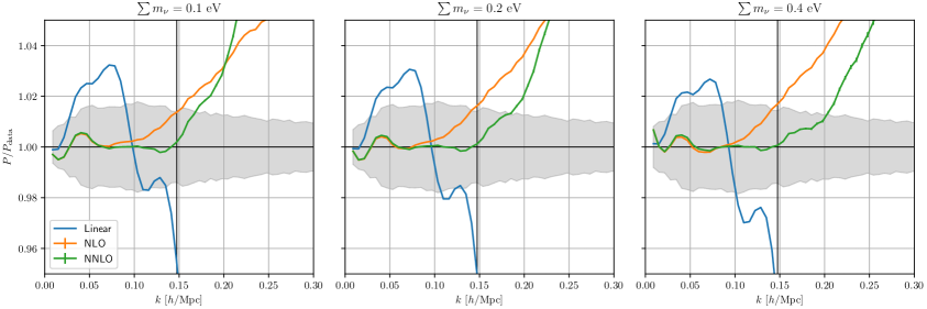
Figure 1: CDM+baryon density power spectrum predictions at linear, next-to-leading- and next-to-next-to-leading order in perturbation theory, normalized to Quijote N-body results, for three neutrino masses $M_{\nu}=0.1$, $0.2$ and $0.4\leavevmode\nobreak\ \mathrm{eV}$. The NLO curve correspond to the 0-parameter model and the NNLO curve to the 2-parameter model defined in Sec. 5, and we use a pivot scale $k_{\mathrm{max}}=0.148h\ \text{Mpc}^{-1}$. The gray area indicates uncertainty from the N-body simulation.

Our work is structured as follows: in the next section we describe how we capture neutrino perturbations in a two-component fluid model and compare it to a simplified approach for the (unrenormalized) density and velocity power spectra in Sec. 3. We detail how we renormalize the power spectrum using an EFT approach in Sec. 4 and compare and calibrate both models to N-body simulations in Sec. 5. We conclude in Sec. 6.

2 Perturbative modelling with massive neutrinos

In this section we briefly review Standard Perturbation Theory (SPT) and the generic extension of it introduced in [57] that can describe cosmologies with multiple species in addition to scale- and time-dependent dynamics. We will apply this framework to cosmologies with massive neutrinos, therefore we next summarize a two-component fluid setup of CDM+baryons and neutrinos introduced in [61] and further developed in [57], which can readily be captured by the extension of SPT. Finally, we compare the two-component fluid model at the linear level to the full neutrino Boltzmann hierarchy.

2.1 Standard perturbation theory

The equations of motion for the density contrast $\delta$ and velocity divergence $\theta=\partial_{i}\mathbf{v}^{i}$ (neglecting vorticity) in Fourier space reads

$$\partial_{\tau}\delta(\mathbf{k},\tau)+\theta(\mathbf{k},\tau) =-\int_{\mathbf{k}_{1},\mathbf{k}_{2}}\delta_{D}(\mathbf{k}-\mathbf{k}_{12})\alpha(\mathbf{k}_{1},\mathbf{k}_{2})\theta(\mathbf{k}_{1},\tau)\delta(\mathbf{k}_{2},\tau)\,,$$

$$\partial_{\tau}\theta(\mathbf{k},\tau)+\mathcal{H}\theta(\mathbf{k},\tau)+\frac{3}{2}\mathcal{H}^{2}\Omega_{m}\delta(\mathbf{k},\tau) =-\int_{\mathbf{k}_{1},\mathbf{k}_{2}}\delta_{D}(\mathbf{k}-\mathbf{k}_{12})\beta(\mathbf{k}_{1},\mathbf{k}_{2})\theta(\mathbf{k}_{1},\tau)\theta(\mathbf{k}_{2},\tau)\,,$$ (2.1)

where $\tau$ is conformal time, $\mathcal{H}=\mathop{}\!{\operator@font d}\ln a/\mathop{}\!{\operator@font d}\tau$ the conformal Hubble rate and $\Omega_{m}$ the time-dependent matter density parameter. We introduced the shorthand notations $\mathbf{k}_{12}=\mathbf{k}_{1}+\mathbf{k}_{2}$ and $\int_{\mathbf{k}}=\int\mathop{}\!{\operator@font d}^{3}\mathbf{k}$ and used $\delta_{D}$ to denote the Dirac delta function. The mode coupling functions are

$$\alpha(\mathbf{k}_{1},\mathbf{k}_{2})=1+\frac{\mathbf{k}_{1}\cdot\mathbf{k}_{2}}{k_{1}^{2}}\,,\quad\beta(\mathbf{k}_{1},\mathbf{k}_{2})=\frac{(\mathbf{k}_{1}+\mathbf{k}_{2})^{2}(\mathbf{k}_{1}\cdot\mathbf{k}_{2})}{2k_{1}^{2}k_{2}^{2}}\,,$$ (2.2)

as usual. In SPT one assumes that the anisotropic stress of the fluid vanishes. We also make this assumption here initially, but will relax it when discussing an effective field theory setup in Sec. 4.

The equations of motion can be written in a compact form after defining the tuple $\psi=(\delta,-\theta/\mathcal{H}f)$ and using $\eta=\log D$, with $D$ and $f$ being the linear growth factor and growth rate, respectively, thus [20]:

$$\partial_{\eta}\psi_{a}(\mathbf{k},\eta)+\Omega_{ab}(\eta)\psi_{b}(\mathbf{k},\eta)=\int_{\mathbf{k}_{1},\mathbf{k}_{2}}\delta_{D}(\mathbf{k}-\mathbf{k}_{12})\gamma_{abc}(\mathbf{k},\mathbf{k}_{1},\mathbf{k}_{2})\psi_{b}(\mathbf{k}_{1},\eta)\psi_{c}(\mathbf{k}_{2},\eta)\,.$$ (2.3)

The matrix $\Omega_{ab}$ governing the linear evolution is given by

$$\Omega_{ab}(\eta)=\begin{pmatrix}0&-1\\ -\frac{3}{2}\frac{\Omega_{m}}{f^{2}}&\frac{3}{2}\frac{\Omega_{m}}{f^{2}}-1\end{pmatrix}\,,$$ (2.4)

and the only non-zero components of the non-linear vertex are $\gamma_{121}(\mathbf{k},\mathbf{k}_{1},\mathbf{k}_{2})=\alpha(\mathbf{k}_{1},\mathbf{k}_{2})$ and $\gamma_{222}(\mathbf{k},\mathbf{k}_{1},\mathbf{k}_{2})=\beta(\mathbf{k}_{1},\mathbf{k}_{2})$.

In SPT one typically adopts the Einstein–de-Sitter (EdS) approximation, in which $\Omega_{m}/f^{2}=1$ so that the $\Omega_{ab}$-matrix becomes time-independent. This approximation greatly simplifies Eq. (2.3), allowing for analytic solutions order by order. Only the decaying mode is affected by changes in the ratio $\Omega_{m}/f^{2}$ and moreover the ratio only departs significantly from one at late times, $z\lesssim 2$ in $\Lambda$CDM (and also in moderate extensions). Consequently, the EdS-approximation has been shown to work at the percent-level for the power spectrum [66, 67, 57, 68, 70] as well as the bispectrum [69, 39]. In particular, in EFT analyses the departure from EdS can be largely degenerate with counterterms, only leading to a shift in the EFT parameters [68, 39]. In this work we consider schemes with and without the EdS approximation, which we will specify accordingly.

2.2 Extension of SPT

Following [57], we extend SPT by allowing for multiple species in the fluid as well as allowing for a general time- and wavenumber-dependence. More precisely, for an $N$-fluid we collect the density contrast and velocity divergence for each component $i$ into into the field vector $\psi_{a}=(\dotsc,\delta_{i},\theta_{i},\dotsc)$ with the index $a$ running from $1$ to $2N$. In addition, we permit a general dependence on time and wavenumber in the (now $2N\times 2N$) matrix describing the linear evolution $\Omega_{ab}=\Omega_{ab}(|\mathbf{k}|,\eta)$. This extension can capture multiple models beyond $\Lambda$CDM in addition to effective models of clustering dynamics. It has in general no analytic solution however, hence we will mostly need to solve the dynamics numerically.

The equations of motion (2.3) can also in this case be solved perturbatively, at each order furnished by $2N$ kernels $F_{a}^{(n)}$ labeled by the index $a$ at order $n$:

$$\psi_{a}(\mathbf{k},\eta)=\sum_{n=1}^{\infty}\int_{\mathbf{q}_{1},\dotsc,\mathbf{q}_{n}}\delta_{D}(\mathbf{k}-\mathbf{q}_{1\cdots n})\,\mathrm{e}^{n\Delta\eta}\,F_{a}^{(n)}(\mathbf{q}_{1},\dotsc,\mathbf{q}_{n};\eta)\,\delta_{0}(\mathbf{q}_{1};\eta_{\mathrm{ini}})\dotsb\delta_{0}(\mathbf{q}_{n};\eta_{\mathrm{ini}})\,,$$ (2.5)

where $\Delta\eta\equiv\eta-\eta_{\mathrm{ini}}$ and $\delta_{0}$ is an initial condition that we discuss shortly. Note that due to the assumed non-trivial time-dependence in the dynamics, we allow for a dependence on $\eta$ in addition to the wavenumbers $\mathbf{q}$ for the kernels. Inserting this solution into Eq. (2.3) yields the following recursive solution at $n$-th order in perturbation theory:

$$(\partial_{\eta}+n)F_{a}^{(n)}(\mathbf{q}_{1},\dotsc,\mathbf{q}_{n};\eta)+\Omega_{ab}(k,\eta)F_{b}^{(n)}(\mathbf{q}_{1},\dotsc,\mathbf{q}_{n};\eta)$$

$$= \sum_{m=1}^{n-1}\Big{[}\gamma_{abc}(\mathbf{k},\mathbf{q}_{1\dotsb m},\mathbf{q}_{m+1\dotsb n})F_{b}^{(m)}(\mathbf{q}_{1},\dotsc,\mathbf{q}_{m};\eta)F_{c}^{(n-m)}(\mathbf{q}_{m+1},\dotsc,\mathbf{q}_{n};\eta)\Big{]}_{\rm sym.}\,.\quad$$ (2.6)

Here, $\mathbf{k}=\sum_{i}\mathbf{q}_{i}$, and the right hand side is understood to be symmetrized with respect to all permutations exchanging momenta in the $\{\mathbf{q}_{1},\dotsc,\mathbf{q}_{m}\}$ set with momenta in the $\{\mathbf{q}_{m+1},\dotsc,\mathbf{q}_{n}\}$ set and normalized to the number of permutations.

Note that setting $N=1$ and using the $\Omega_{ab}$-matrix from Eq. (2.4) with $\Omega_{m}/f^{2}=1$ (EdS approximation) in Eq. (2.6), we recover in the limit $\eta_{\mathrm{ini}}\to-\infty$ the usual kernel recursion relations with the replacements $F_{1}^{(n)}\to F_{n}$ and $F_{2}^{(n)}\to G_{n}$.

We still need to specify suitable initial conditions in order to solve the above equations. Taking $\eta_{\mathrm{ini}}$ after recombination but long before non-linearities become important at the scales of interest, we assume that the initial conditions for each fluid component is correlated, so that

$$\psi_{a}(\mathbf{k},\eta_{\mathrm{ini}})=F_{a}^{(1)}(k,\eta_{\mathrm{ini}})\,\delta_{0}(\mathbf{k})\,,$$ (2.7)

which holds for adiabatic initial conditions. Furthermore, we assume that $\delta_{0}$ is a Gaussian random field, so that we only need to specify the initial linear power spectrum $\langle\delta_{0}(\mathbf{k})\delta_{0}(\mathbf{k}^{\prime})\rangle=\delta_{D}(\mathbf{k}+\mathbf{k}^{\prime})P_{0}(k)$ in order to compute correlations of $\psi_{a}$’s. The initial linear kernels $F_{a}^{(1)}(k,\eta_{\mathrm{ini}})$ impose the relative normalization for each perturbation and wavenumber. Deep in the linear regime $\eta_{\mathrm{ini}}\to\infty$ the higher order initial kernels can be set to zero. In practice however, using $\eta_{\mathrm{ini}}$ after recombination, we find that those $n>1$ initial conditions work poorly because they excite transient solutions that do not entirely decay by $\eta=0$ ($z=0$). We return to this issue below.

We are ultimately interested in the statistical properties of the fields $\psi_{a}(\mathbf{k},\eta)$, in particular auto- and cross power spectra

$$\langle\psi_{a}(\mathbf{k},\eta)\psi_{b}(\mathbf{k}^{\prime},\eta)\rangle=\delta_{D}(\mathbf{k}+\mathbf{k}^{\prime})P_{ab}(k,\eta)\,.$$ (2.8)

The perturbative expansion (2.5) combined with the Wick theorem yields as a result the loop expansion of the power spectrum

$$P_{ab}(k,\eta)=P_{ab}^{\rm lin}(k,\eta)+P_{ab}^{\text{1-loop}}(k,\eta)+P_{ab}^{\text{2-loop}}(k,\eta)+\dots\,.$$ (2.9)

To compute loop corrections, we employ the numerical algorithm described in [57] (see also [58, 59, 60]). In short, at $L$-loop it consists of integrating over $L$ loop momenta using Monte Carlo integration (with CUBA [78]) where at every integration point a set of $(2L+1)$-order kernels needs to be evaluated using the recursion relation (2.6). In general, there is no analytic solution of Eq. (2.6), therefore we solve for the kernels numerically. We refer to [57] for further details on the algorithm.

2.3 Two-component fluid: CDM+baryons and massive neutrinos

We will employ the hybrid two-component fluid setup described in [57] to model structure formation in massive neutrino cosmologies. In the following, we repeat the main elements of this setup for convenience, but refer to [57] for details of the implementation.

In the hybrid two-component fluid model, the system is described linearly by the full Boltzmann hierarchy until some intermediate redshift $z_{\mathrm{match}}$, after which the evolution is mapped onto a two-component fluid, suitable for computing non-linear corrections (see also [61]). Baryons and CDM comprise jointly one fluid component, which is coupled to the second component, the neutrinos, via gravity. A fluid description of massive neutrinos is suitable at late times because the coupling to higher moments in the Boltzmann hierarchy is suppressed by powers of $T_{\nu}/m_{\nu}$. We may therefore follow only the lowest moments of the hierarchy for the neutrinos, with an effective sound velocity to capture free-streaming. We show below that this only leads to sub-percent differences compared to the full hierarchy. The CDM+baryon component is treated both as a perfect, pressureless fluid (SPT) as well as an imperfect fluid with corrections to the effective stress tensor (EFT).

We consider three massive neutrino cosmologies with $M_{\nu}\equiv\sum_{i}m_{\nu_{i}}=0.1$, $0.2$ and $0.4\leavevmode\nobreak\ \mathrm{eV}$. In all models we assume that the neutrinos are degenerate, each with mass $M_{\nu}/3$. This approximation works well because cosmological observables are very insensitive to the neutrino mass hierarchy except for the total mass, see e.g. [79]. Furthermore, we choose a matching redshift $z_{\mathrm{match}}=25$, which for the neutrino masses of consideration is well after the non-relativistic transition

$$z_{\mathrm{nr}}=1890\frac{m_{\nu}}{1\leavevmode\nobreak\ \mathrm{eV}}\,,$$ (2.10)

in addition to being sufficiently earlier than the point at which non-linearities become important, $z\lesssim 10$.

The weighted density contrast for the CDM+baryon fluid component reads

$$\delta_{\mathrm{cb}}=\frac{f_{\mathrm{b}}\delta_{\mathrm{b}}+f_{\mathrm{cdm}}\delta_{\mathrm{cdm}}}{f_{\mathrm{b}}+f_{\mathrm{cdm}}}\,,$$ (2.11)

with $f_{i}\equiv\Omega_{i}/\Omega_{\mathrm{tot}}$, and similarly for the velocity divergence. We collect the density contrasts and (suitably rescaled) velocity divergences of both fluid components into a vector 

$$\psi_{a}=\left(\delta_{\mathrm{cb}}\,,\quad-\frac{\theta_{\mathrm{cb}}}{\mathcal{H}f}\,,\quad\delta_{\nu}\,,\quad-\frac{\theta_{\nu}}{\mathcal{H}f}\right).$$ (2.12)

The equations of motion for the two-component fluid are given by Eq. (2.3) with

$$\Omega_{ab}(k,\eta)=\begin{pmatrix}0&-1&0&0\\ -\frac{3}{2}\frac{\Omega_{m}}{f^{2}}(1-f_{\nu})&\frac{3}{2}\frac{\Omega_{m}}{f^{2}}-1&-\frac{3}{2}\frac{\Omega_{m}}{f^{2}}f_{\nu}&0\\ 0&0&0&-1\\ -\frac{3}{2}\frac{\Omega_{m}}{f^{2}}(1-f_{\nu})&0&-\frac{3}{2}\frac{\Omega_{m}}{f^{2}}[f_{\nu}-k^{2}c_{s,\mathrm{eff}}^{2}(k,\eta)]&\frac{3}{2}\frac{\Omega_{m}}{f^{2}}-1\end{pmatrix}\,,$$ (2.13)

and the non-zero components of the vertex $\gamma_{abc}$ being

$$\gamma_{121}(\mathbf{k},\mathbf{k}_{1},\mathbf{k}_{2})=\gamma_{343}(\mathbf{k},\mathbf{k}_{1},\mathbf{k}_{2})\equiv\alpha(\mathbf{k}_{1},\mathbf{k}_{2})\,,$$

$$\gamma_{222}(\mathbf{k},\mathbf{k}_{1},\mathbf{k}_{2})=\gamma_{444}(\mathbf{k},\mathbf{k}_{1},\mathbf{k}_{2})\equiv\beta(\mathbf{k}_{1},\mathbf{k}_{2})\,.$$ (2.14)

In the part of the evolution matrix $\Omega_{ab}$ describing the neutrino dynamics, we introduced the effective neutrino sound velocity $c_{s,\mathrm{eff}}^{2}$. This term captures the free-streaming of the neutrinos $c_{s}^{2}=\delta P_{\nu}/\delta\rho_{\nu}$ as well as the neutrino anisotropic stress $\sigma_{\nu}$:

$$c_{s,\mathrm{eff}}^{2}(k,\eta)\equiv\frac{1}{k_{\mathrm{FS}}^{2}(k,\eta)}=\frac{2}{3\Omega_{m}\mathcal{H}^{2}}\left[c_{s}^{2}(k,\eta)-\frac{\sigma_{\nu}(k,\eta)}{\delta_{\nu}(k,\eta)}\right]\,,$$ (2.15)

where we defined the associated effective free-streaming wavenumber $k_{\mathrm{FS}}$. We compute the terms in the bracket in linear theory, however in a manner that is informed about the complete neutrino distribution function, including all higher moments (see [57]).

The equations for the two-component fluid are precisely of the form that can be solved by the extension of SPT discussed above. We expand $\psi_{a}$ in powers of $\delta_{0}=\delta_{\mathrm{cb}}(\eta_{\mathrm{match}})$ using Eq. (2.5). The accompanying kernels are solutions of Eq. (2.6), with $\Omega_{ab}$ and $\gamma_{abc}$ from Eqs. (2.13) and (2.14). We find that we need to be cautious in choosing initial conditions for the kernel hierarchy at the matching redshift; one easily excites transient solutions that do not entirely decay away by $\eta=0$. Ultimately, we opt for numerically finding the growing mode solution for the kernels with fixed $\Omega_{ab}(k)=\Omega_{ab}(k,\eta_{\mathrm{match}})$ and using this as initial condition. This method is described more comprehensively in [57]. We check that this initial condition matches at the linear level the transfer functions from the Boltzmann solver CLASS [80] for the wavenumbers of interest, and that we obtain the same linear power spectrum at $z=0$ (see below).

The total matter power spectrum is the sum of the weighted auto spectra for each component as well as the cross-spectrum,

$$P_{\mathrm{m},\mathrm{m}}=(1-f_{\nu})^{2}P_{\mathrm{cb},\mathrm{cb}}+2(1-f_{\nu})f_{\nu}P_{\mathrm{cb},\nu}+f_{\nu}^{2}P_{\nu,\nu}\,.$$ (2.16)

The neutrino energy fraction is $f_{\nu}=0.75$, $0.15$ and $0.3\%$ (constant for $z\ll z_{\mathrm{nr}}$) for the three models with $M_{\nu}=0.1$, $0.2$ and $0.4\leavevmode\nobreak\ \mathrm{eV}$, respectively. For wavenumbers larger than the neutrino free-streaming scale $k_{\mathrm{FS}}\sim 0.01\leavevmode\nobreak\ h/\mathrm{Mpc}$, neutrinos are hardly captured in gravitational wells and the neutrino spectra are suppressed compared to $P_{\mathrm{cb},\mathrm{cb}}$. In total, the first term in Eq. (2.16) gives the dominant contribution to the matter power spectrum. Nevertheless, via the backreaction on the gravitational potential, the presence of massive neutrinos leads to a reduction of growth of the CDM+baryon fluid. At the linear level, the relative suppression of the matter power spectrum between a model with massive neutrinos and one without (with $\Omega_{\mathrm{cdm}}$ tuned so that $\Omega_{m}$ is the same) is the well-known $-8f_{\nu}$ [9].

In Fig. 2, we compare the two-fluid scheme with the full solution using the Boltzmann hierarchy (CLASS, with maximum neutrino multipole $l_{\mathrm{max}}=17$) at the linear level. The matter power spectra have sub-permille agreement for $k>0.03\leavevmode\nobreak\ h/\mathrm{Mpc}$ for all neutrino masses. For very low wavenumber, $k\to 10^{-3}\leavevmode\nobreak\ h/\mathrm{Mpc}$ there are percent-level deviations. These arise because at the matching redshift $z_{\mathrm{match}}=25$, the wavenumbers have not yet completely reached the growing mode after entering the horizon, while the two-fluid model initial condition assumes that all scales already reside in the growing mode. In addition, for scales close to Hubble, relativistic corrections become important. Nevertheless, these large scales have negligible impact on loop corrections for a realistic power spectrum.

The neutrino auto power spectrum agrees better than 1% for scales $k\sim 0.01$ – $0.1\leavevmode\nobreak\ h/\mathrm{Mpc}$. On smaller scales the difference increase, however in this region errors from the truncation of the Boltzmann hierarchy (choice of $l_{\mathrm{max}}$) also become significant. We see that the deviation of the neutrino spectrum has a minimal effect on the total matter power spectrum, whose dominant contribution is the CDM+baryon component.

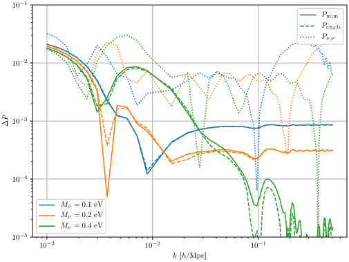
Figure 2: Relative difference between the linear power spectra computed using the two-fluid model and using the full Boltzmann hierarchy for the neutrino perturbation (CLASS), $\Delta P=|1-P/P_{\mathrm{CLASS}}|$. The solid, dashed and dotted lines correspond to $P_{\mathrm{m},\mathrm{m}}$, $P_{\mathrm{cb},\mathrm{cb}}$ and $P_{\nu,\nu}$, respectively, while the blue, orange and green lines correspond to $M_{\nu}=0.1$, $0.2$, and $0.4\leavevmode\nobreak\ \mathrm{eV}$, respectively.

3 Effect of neutrino perturbations on density and velocity spectra

Having set up the formalism and procedure for computing non-linear corrections taking neutrino perturbations into account beyond the linear level, we proceed in this section to comparing it to simplified treatments. We consider the bare density- and velocity power spectra, and leave a comparison of the renormalized power spectra to Sec. 5. Furthermore, we assess to which extent the effect of free-streaming neutrinos is degenerate with the primordial amplitude of fluctuations at one- and two-loop on BAO scales.

The schemes for describing the growth of structure in presence of massive neutrinos that we will consider in this work in increasing order of complexity are:

1. EdS-SPT scheme (1F). The impact of neutrinos is only taken into account at the linear level. Therefore, the only species modelled non-linearly by the fluid Eqs. (2.3) is CDM+baryons (joint fluid). In addition, the ratio $\Omega_{m}/f^{2}$ is approximated to 1 so that analytical EdS-SPT kernels may be used. This approach is frequently used in the literature because of its simplicity and efficiency, the latter being particularly favorable for data analysis and parameter scans.

2. One-fluid scheme (1F+). Equivalent to the 1F-scheme, but relaxing the EdS approximation by including the time-dependence of $\Omega_{m}/f^{2}$. This scheme is included in order to estimate to what degree the EdS approximation is the source of inaccuracies when comparing 1F and 2F.

3. Two-fluid scheme (2F). Baryons+CDM and neutrinos are both modelled beyond the linear theory in the two-component fluid setup. The time- and scale-dependence of the dynamics both arising from the departure from EdS at late times as well as neutrino free-streaming are captured by solving the kernel hierarchy (2.6) numerically, with the linear evolution and non-linear vertices given by Eqs. (2.13) and (2.14), respectively.

For the 1F and 1F+ schemes, we use the linear power spectrum at $z=0$ (from CLASS) as input to the loop correction calculations. The 2F scheme however, captures also accurately the linear evolution (see discussion above), thus we take the linear power spectrum at $z_{\mathrm{match}}=25$ as input. The increasing complexity of the different schemes leads to longer processing times; in Table 1 we list the approximate times to compute one integration point on one core on a laptop at one- and two-loop in each scheme. A typical calculation of a loop correction for a single external wavenumber entails $\mathcal{O}(10^{6})$ integral evaluations.

Table 1: Approximate time in microseconds to compute one integration point (the integrand for a fixed set of integration variables) at one- and two-loop in the different schemes. Measured on a laptop using one core.

	EdS-SPT (1F)	One-fluid (1F+)	Two-fluid (2F)
1-loop	3	620	1600
2-loop	50	5400	15000

3.1 Comparison

To address the accuracy of treating neutrinos only linearly as well as the EdS approximation, we compare the 1F and 2F schemes for the CDM+baryon density and velocity power spectra at $z=0$. We consider the power spectrum both at NLO (linear + one-loop) and NNLO (linear + one-loop + two-loop), without EFT corrections (we repeat the comparison including these in Sec. 5).

The comparison is presented in Fig. 3. In the leftmost panel we show the density auto spectrum $P_{\delta_{\mathrm{cb}},\delta_{\mathrm{cb}}}$ in the 1F and 1F+ schemes, normalized to the 2F result. At one-loop (dashed lines), the 1F scheme deviates at most by $0.5\%$ from the full 2F solution, while at two-loop (solid lines) the deviation exceeds one percent at $k\simeq 0.17\leavevmode\nobreak\ h\ \text{Mpc}^{-1}$ and grows as the two-loop correction becomes increasingly significant. A similar comparison was done for different neutrino masses in [57], and it is reassuring to see consistent results. Since the deviations are roughly independent of neutrino mass and there is insignificant difference between the 1F+ (EdS approximation relaxed) and 2F schemes at two-loop (dotted lines), we conclude that the main source of inaccuracy for the density spectrum comes from the EdS approximation.

The middle and right panels display the same comparison for the cross spectrum $P_{\delta_{\mathrm{cb}},\theta_{\mathrm{cb}}}$ and velocity spectrum $P_{\theta_{\mathrm{cb}},\theta_{\mathrm{cb}}}$. In contrast to the density spectrum, they show a clear dependence on the neutrino mass in the fractional difference. Moreover, the deviations of the 1F and 1F+ schemes from the full 2F solution are very similar for $P_{\theta_{\mathrm{cb}},\theta_{\mathrm{cb}}}$, indicating that the main error comes from neglecting the effect of non-linear neutrino perturbations. It is not too surprising that this effect is larger on the fluid velocity than the density contrast: for scales smaller than the free-streaming scale the growing mode for the CDM+baryon component is approximately $(1,1-3/5\,f_{\nu})$ in the 2F scheme, while it remains $(1,1)$ in 1F (and 1F+). Therefore, there is an extra suppression for the velocity field compared to the density field, in addition to the change of the growth factor. Nevertheless, the deviation for the smallest neutrino mass $M_{\nu}=0.1\leavevmode\nobreak\ \mathrm{eV}$ is less than a percent at two-loop for $k\lesssim 0.15$ and $0.2\leavevmode\nobreak\ h\ \text{Mpc}^{-1}$ for the cross- and velocity spectra, respectively. We note that for wavenumbers $k\gtrsim 0.2\leavevmode\nobreak\ h\ \text{Mpc}^{-1}$ the two-loop correction is of the order of the one-loop correction, signalling the breakdown of perturbation theory. Finally, for the velocity spectra it is curious to see that the deviations of 1F to 2F for the one- and two-loop corrections go in opposite directions, thus adding the two-loop seemingly improves the agreement.

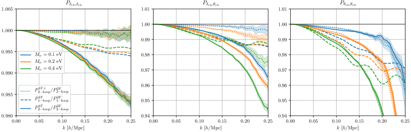
Figure 3: Comparison of the 1F, 1F+ and 2F schemes for the CDM+baryon density and velocity spectra. We show the power spectrum at one-loop (dashed lines) and two-loop (solid lines) in the 1F scheme, divided by that from the 2F scheme. The dotted lines correspond to the 1F+ scheme normalized to the 2F scheme, at two-loop order. Shaded regions indicate uncertainty from the Monte Carlo integration. Left: density auto spectrum, middle: density-velocity cross spectrum and right: velocity auto spectrum.

3.2 Degeneracy with amplitude of fluctuations

The suppression of power on scales smaller than the neutrino free-streaming scale is largely degenerate with a change of the clustering amplitude $A_{s}$. This may pose a major limitation on constraining the neutrino mass with large-scale structure [81, 82, 83, 84]. The complication is somewhat mitigated by measuring at different redshifts, including higher-order statistics [17, 77] and by redshift-space distortions [34]. Moreover, the degeneracy can be broken by including other probes, such as CMB data.

In this light, we check to what extent we can reproduce our results for the 2F matter power spectra in massive neutrino models using massless models by adjusting $A_{s}$. To isolate the effect of neutrino suppression and overall amplitude, we use the 1F+ scheme for the massless models. Furthermore, we remove completely the double-hard limit of the two-loop corrections, which otherwise yields a large contribution at the scales of interest (after renormalization this contribution is considerably reduced). In Sec. 4 we go into details on this procedure and include EFT corrections to renormalize the power spectrum. For simplicity, we set $A_{s}^{\prime}=(1-8f_{\nu})A_{s}$ to mimic neutrino free-streaming suppression in the massless models. The results are shown in Fig. 4. For the lowest neutrino mass, the massive and modified massless models agree within a percent. As the characteristic free-streaming wavenumber increases for larger neutrino mass, it becomes more difficult to reconstruct the shape of the massive neutrino non-linear power spectrum with a change of $A_{s}$. The shape dependence of the linear suppression is more prominent at $k\simeq 0.1$ – $0.2h\ \text{Mpc}^{-1}$ and due to mode-coupling, the loop-corrections are affected beyond just a rescaling by the presence of the neutrinos.

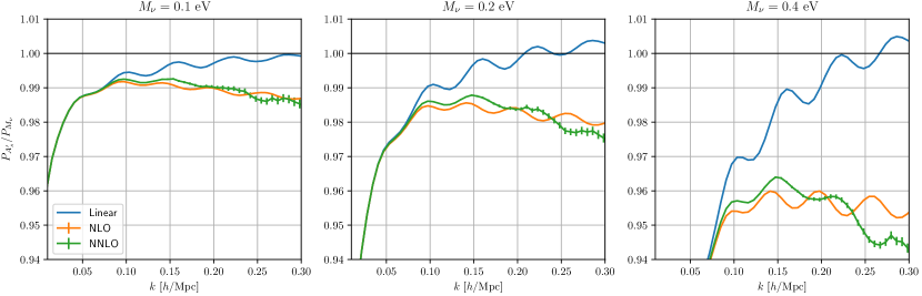
Figure 4: Comparison of the total matter power spectrum in massive neutrino models and massless models with the amplitude of fluctuations changed. We show massless models with $A_{s}^{\prime}=(1-8f_{\nu})A_{s}$ normalized to massive models with amplitude $A_{s}$ for the linear (blue), NLO (orange) and NNLO (green) power spectrum. To isolate the effect of the neutrinos, we compute the massless model in the 1F+ scheme and the massive model in the 2F scheme. Errorbars indicate uncertainty from Monte Carlo integration.

4 Effective field theory setup

In order to precisely assess the performance of the simplified treatment of neutrinos (1F) and the full two-fluid solution (2F) versus N-body simulations, we need to take into account EFT corrections. In this section we elaborate on the EFT setup we employ for obtaining a renormalized CDM+baryon power spectrum at next-to-next-to-leading order.

In the effective theory approach, long wavelength fluctuations are modelled perturbatively while systematically taking into account the impact of short wavelengths [22, 23]. This is done by coarse-graining the fluid, leading to a modified Euler equation with an effective stress tensor that in addition to the microscopic stress includes corrections from coarse-grained products of short fluctuations. In the notation introduced in Sec. 2, the equations of motion (2.3) in the two-fluid model are modified as

$$\partial_{\eta}\psi_{a}(\mathbf{k},\eta)+\Omega_{ab}(\mathbf{k},\eta)\psi_{b}(\mathbf{k},\eta) =\int_{\mathbf{k}_{1},\mathbf{k}_{2}}\delta_{D}(\mathbf{k}-\mathbf{k}_{12})\gamma_{abc}(\mathbf{k},\mathbf{k}_{1},\mathbf{k}_{2})\psi_{b}(\mathbf{k}_{1},\eta)\psi_{c}(\mathbf{k}_{2},\eta)$$

$$\phantom{=}+\delta_{a2}^{(K)}\,\tau_{\theta_{\mathrm{cb}}}(\mathbf{k})+\delta_{a4}^{(K)}\,\tau_{\theta_{\nu}}(\mathbf{k})\,,$$ (4.1)

where $\delta_{ij}^{(K)}$ is the Kronecker delta, and the effective stress terms are defined equivalently for the CDM+baryon and neutrino fluid in real space as

$$\tau_{\theta}=\partial_{i}\frac{1}{1+\delta}\partial_{j}\tau^{ij}\,.$$ (4.2)

The effective stress tensor $\tau^{ij}$ can in the effective theory be split into a deterministic and stochastic contribution; the deterministic part can be modelled in terms of the perturbative solution, while the stochastic part is uncorrelated with the long modes and must be modelled statistically. Due to momentum conservation, the deterministic part must scale as the density contrast times $k^{2}$ as $k\to 0$, while the stochastic power spectrum vanishes faster than $k^{4}$ in this limit [85, 86]. Therefore, we neglect the stochastic contribution in this work.

In the effective theory the deterministic part of the stress tensor is not described from first principles, but written down as a sum of all possible operators allowed by symmetries, with a priori unknown EFT coefficients that must be fitted to simulations or marginalized over in data analysis. Due to Galilean invariance and the equivalence principle, the operators are restricted to gradients and products of the building blocks $\partial^{i}\partial^{j}\Phi$ and $\partial^{i}\mathbf{v}^{j}$, where $\Phi$ is the rescaled gravitational potential satisfying $\Delta\Phi=\delta$. At leading order in gradients and number of factors of fields, the effective stress term is [86]

$$\tau_{\theta}\big{|}_{\mathrm{1}}=d_{\delta}^{2}\,\Delta\delta^{(1)}+d_{\theta}^{2}\,\Delta\theta^{(1)}\,,$$ (4.3)

where $d_{\delta}^{2}$ and $d_{\theta}^{2}$ are (time-dependent) EFT coefficients, and $\delta^{(1)}$ and $\theta^{(1)}$ are the linear solutions in perturbation theory. In massless neutrino cosmologies, they are related by $\delta^{(1)}=-\theta^{(1)}/\mathcal{H}f$, so that the sum above can be reduced to $d^{2}\Delta\delta_{(1)}$ with $d^{2}=d_{\delta}^{2}-d_{\theta}^{2}/\mathcal{H}f$. This is not the case for massive neutrino models, due to free-streaming, therefore we in principle need to write down

$$\tau_{\theta_{\mathrm{cb}}}\big{|}_{\mathrm{1}}=\sum_{i=1}^{4}d_{\mathrm{cb},i}^{2}\,\Delta\psi_{i}^{(1)}\qquad\text{and}\qquad\tau_{\theta_{\nu}}\big{|}_{\mathrm{1}}=\sum_{i=1}^{4}d_{\nu,i}^{2}\,\Delta\psi_{i}^{(1)}$$ (4.4)

in the two-fluid model with EFT coefficients $d_{\mathrm{cb},i}$, $d_{\nu,i}$. This leads to a counterterm CDM+baryon density field

$$\tilde{\psi}_{1}^{(1)}\equiv\tilde{\delta}_{\mathrm{cb}}^{(1)}=k^{2}\sum_{i=1}^{4}\mathsf{d}_{i}^{2}\,\psi_{i}^{(1)}$$ (4.5)

in Fourier space. Each coefficient $\mathsf{d}_{i}$ depends on a linear combination of both sets of coefficients $d_{\mathrm{cb},i}$, $d_{\nu,i}$ because the linear propagation after the insertion of the sources $\tau_{\theta_{\mathrm{cb}}}$ and $\tau_{\theta_{\nu}}$ mixes the contributions from the four components.

In practice, we are interested in weakly non-linear scales $k\simeq 0.1h\ \text{Mpc}^{-1}$, and assume a large scale separation $k_{\mathrm{FS}}\ll k\ll k_{\mathrm{NL}}$, where the non-linear scale is $k_{\mathrm{NL}}\sim 0.3h\ \text{Mpc}^{-1}$. As we return to below, this assumption is justified for $M_{\nu}=0.1$ and $0.2\leavevmode\nobreak\ \mathrm{eV}$ but begins to break down for $M_{\nu}=0.4\leavevmode\nobreak\ \mathrm{eV}$. In particular, the linear CDM+baryon density contrast and (rescaled) velocity divergence can be related by a constant factor far below the free-streaming scale: we have approximately $\psi_{2}^{(1)}=(1-3/5\,f_{\nu})\psi_{1}^{(1)}$, see the left panel of Fig. 5 (the linear solutions are $\psi_{i}^{(1)}\propto F_{i}^{(1)}\delta_{\mathrm{cb}}(\eta_{\mathrm{ini}})$). Furthermore, based on the expectation that $\mathsf{d}_{i}^{2}/k_{\mathrm{NL}}^{2}=\mathcal{O}(1)$ and that the neutrino perturbations are more than an order of magnitude smaller than the CDM+baryon ones around the scales of interest – see the right panel of Fig. 5 – we neglect the contribution from the $\psi_{3}^{(1)}$- and $\psi_{4}^{(1)}$-terms. Note also that the sound velocity in the microscopic part of the $\tau_{\nu}^{ij}$ stress tensor is already captured in the 2F model, as defined in Eq. (2.15). In total, the leading CDM+baryon counterterm density can be written as

$$\tilde{\psi}_{1}^{(1)}(\eta)=\mathrm{e}^{2\Delta\eta}\gamma_{1}(\eta)\,k^{2}\psi_{1}^{(1)}(\eta_{\mathrm{ini}})\,,$$ (4.6)

where $\gamma_{1}$ is an EFT parameter and we extracted the overall growth $\mathrm{e}^{2\Delta\eta}$ for convenience. Since we will determine $\gamma_{1}$ via calibration to N-body simulations, its explicit relation to the coefficients $\mathsf{d}_{i}$ and kernels $F_{i}^{(1)}(\eta)$ is not important.

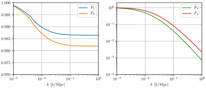
Figure 5: Linear kernels $F_{a}^{(1)}$ at $z=0$ for $M_{\nu}=0.1\leavevmode\nobreak\ \mathrm{eV}$.

4.1 Renormalization of the one-loop correction

To assess whether the counterterms from the effective stress term in the EFT can cure the cutoff-dependence of SPT (also in the 2F scheme), we study its UV sensitivity, starting with the one-loop correction. In the EdS approximation (1F scheme), the leading contribution (i.e. at leading power in the gradient expansion $k^{2}/k_{\mathrm{NL}}^{2}$) to the SPT one-loop power spectrum for hard loop momentum $q\to\infty$ is

$$P_{1L}^{h}(k,\eta)=-2\mathrm{e}^{4\Delta\eta}k^{2}P_{0}(k)\,c\,\frac{4\pi}{3}\int^{\Lambda}\mathop{}\!{\operator@font d}q\,P_{0}(q)=-2\mathrm{e}^{4\Delta\eta}k^{2}P_{0}(k)\,c\,\sigma_{\mathrm{d}}^{2}\,,$$ (4.7)

where

$$\sigma_{\mathrm{d}}^{2}=\frac{4\pi}{3}\int^{\Lambda}\mathop{}\!{\operator@font d}q\,P_{0}(q)$$ (4.8)

is the displacement dispersion. $P_{0}$ is the input linear power spectrum from the initial condition, as defined above. From here on we will only consider the CDM+baryon power spectrum, and we drop the cb subscript for brevity. Due to momentum conservation, the kernels $F^{(n)}(\mathbf{q}_{1},\dotsc,\mathbf{q}_{n})$ scale as $k^{2}$ when the sum $\mathbf{k}=\sum_{i}\mathbf{q}_{i}$ goes to zero. Therefore, the dominant contribution to the hard limit above comes from the diagram containing $F^{(3)}$, and the coefficient $c$ is given by

$$c=9\int\frac{\mathop{}\!{\operator@font d}\Omega_{q}}{4\pi}\left(\lim_{q\to\infty}\,\frac{q^{2}}{k^{2}}F^{(3)}(\mathbf{k},\mathbf{q},-\mathbf{q})F^{(1)}(\mathbf{k})\right)=\frac{61}{210}\,.\qquad\left[\text{1F scheme}\right]$$ (4.9)

We expect the $k^{2}$-scaling guaranteed by momentum conservation also in the 2F scheme, but the $c$-coefficient can change and acquire a time-dependence inherited from the kernels. To analyse the UV and determine $c(\eta)$ in the 2F model, we compute the hard limit of the one-loop integral numerically. This can be done as follows: Define the one-loop integrand $\mathsf{p}_{1L}$ by

$$P_{1L}(k,\eta)=\mathrm{e}^{4\Delta\eta}\int^{\Lambda}\mathop{}\!{\operator@font d}q\,q^{2}P_{0}(q)\int\mathop{}\!{\operator@font d}\Omega_{q}\,\mathsf{p}_{1L}(\mathbf{k},\mathbf{q};\eta)\,.$$ (4.10)

It contains the different diagrams contributing to the one-loop correction with the corresponding kernels and an additional linear power spectrum. In the hard limit, the leading contribution to $\mathsf{p}_{1L}$ should scale as $F^{(3)}(\mathbf{k},\mathbf{q},-\mathbf{q})\sim k^{2}/q^{2}$, therefore we can factorize the integration:

$$P_{1L}^{h}(k,\eta)=3\mathrm{e}^{4\Delta\eta}\int\frac{\mathop{}\!{\operator@font d}\Omega_{q}}{4\pi}\left(\lim_{q\to\infty}\,q^{2}\mathsf{p}_{1L}(\mathbf{k},\mathbf{q};\eta)\right)\frac{4\pi}{3}\int^{\Lambda}\mathop{}\!{\operator@font d}qP_{0}(q)\equiv\mathrm{e}^{4\Delta\eta}p_{1L}^{h}(k,\eta)\,\sigma_{\mathrm{d}}^{2}\,.$$ (4.11)

To evaluate $p_{1L}^{h}$, we fix the loop momentum to a large value $q\gg\Lambda$ and integrate over the angle numerically. Comparing to Eq. (4.7), we find

$$c(\eta)=-\frac{p_{1L}^{h}(k,\eta)}{2k^{2}P_{0}(k)}\,.$$ (4.12)

In Fig. 6 we show the results for the $c$-coefficient at $\eta=0$ for the different neutrino masses, using $\Lambda=1h\ \text{Mpc}^{-1}$ and fixing $q=10h\ \text{Mpc}^{-1}$. The constant $c=61/210$ in the 1F scheme is shown for comparison. Furthermore, we display dashed lines where the linear kernel is divided out in order to isolate the scaling of the $F^{(3)}$ kernel in the hard limit, i.e. $c/F_{1}^{(1)}(k)|_{\eta=0}$. We see that the presence of an additional scale, the free-streaming scale $k_{\mathrm{FS}}$, induces a $k$-dependence: $c=c(k^{2}/k_{\mathrm{FS}}^{2})$ . In the limit $k\ll k_{\mathrm{FS}}$, neutrinos behave as dark matter, and the system can be mapped onto a set of standard dark matter fluid equations for which the hard limit yields $c$ constant. We do not recover the 1F limit of $61/210$, because the EdS approximation is relaxed and because the kernel $F^{(3)}(\mathbf{k},\mathbf{q},-\mathbf{q};\eta)$ is sensitive to the dynamics at $q\gg k_{\mathrm{FS}}$ where the growth rate is dampened due to neutrino free-streaming. For the largest neutrino mass with the largest free-streaming wavenumber, this limit is visible around $k=10^{-3}h\ \text{Mpc}^{-1}$ in Fig. 6.

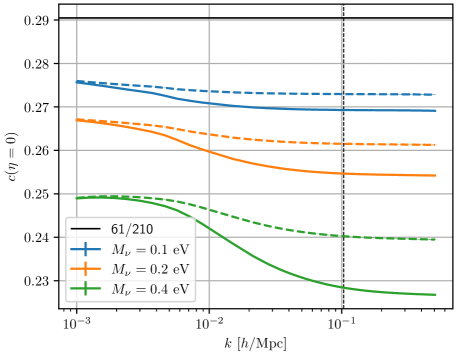
Figure 6: Hard limit of the one-loop correction in the 1F and 2F schemes (for the three neutrino masses), represented by the coefficient $c$ today ($\eta=0$). In the dashed lines the linear kernel is divided out: $c/F_{1}^{(1)}(k)|_{\eta=0}$. The black, dashed line indicates where we read off the value in each model.

On scales much smaller than the free-streaming scale, neutrinos do not cluster and the CDM+baryon and neutrino fluid system effectively decouple. The CDM+baryon fluid is then equivalent to the standard case (1F), with the EdS approximation relaxed and with reduced growth due to the effect of the neutrinos on the background evolution. Hence $c$ approaches a constant for $k\gg k_{\mathrm{FS}}$.

Our aim is to obtain a renormalized power spectrum in the mildly non-linear regime, $k\simeq 0.1h\ \text{Mpc}^{-1}$, therefore we assume a large scale separation $k_{\mathrm{FS}}\ll k\ll q$ . In this limit $c$ is constant, which implies that the counterterm (4.6) can absorb the cutoff dependence of the one-loop correction, as we show explicitly below. For the lowest neutrino masses, we see indeed a plateau in the value of $c$ around $k=0.1h\ \text{Mpc}^{-1}$ in Fig. 6. The measured value is read off at the dashed line and quoted in Tab. 2. For the largest neutrino mass, the assumption of large scale separation $k_{\mathrm{FS}}\ll k$ starts to break down (from Eq. (2.15) we have e.g. $k_{\mathrm{FS}}(k=0.1h\ \text{Mpc}^{-1},\eta=0)=0.07h\ \text{Mpc}^{-1}$), and the plateau emerges only on even smaller scales. Nevertheless, we read off the value of $c$ and include the model in our analysis for illustration. In practice, the limit $k_{\mathrm{FS}}\ll k\ll q$ is well satisfied for relevant values of the sum of neutrino masses.

The counterterm (4.6) gives the additional contribution

$$P_{1L}^{\mathrm{ctr}}(k,\eta;\Lambda)=-2\mathrm{e}^{4\Delta\eta}\,\gamma_{1}(\Lambda)k^{2}P_{0}(k)\,,$$ (4.13)

to the power spectrum, which is exactly of the form to absorb the UV sensitivity (4.7). The renormalized one-loop CDM+baryon power spectrum therefore reads

$$P_{1L}^{\mathrm{ren}}(k,\eta,\Lambda)=P_{1L}(k,\eta;\Lambda)+P_{1L}^{\mathrm{ctr}}(k,\eta;\Lambda)\,.$$ (4.14)

Demanding that the renormalized result is cutoff-independent yields the renormalization group equation

$$0=\frac{\mathop{}\!{\operator@font d}}{\mathop{}\!{\operator@font d}\Lambda}\left[P_{1L}(k,\eta;\Lambda)+P_{1L}^{\mathrm{ctr}}(k,\eta;\Lambda)\right]=-2\mathrm{e}^{4\Delta\eta}k^{2}P_{0}(k)\frac{\mathop{}\!{\operator@font d}}{\mathop{}\!{\operator@font d}\Lambda}\left[c(\eta)\sigma_{\mathrm{d}}^{2}(\Lambda)+\gamma_{1}(\Lambda)\right]$$ (4.15)

at leading power in gradients $k^{2}/k_{\mathrm{NL}}^{2}$, which has the solution

$$\gamma_{1}(\Lambda)=\overline{\gamma}_{1}+\frac{4\pi c}{3}\int_{\Lambda}^{\infty}\mathop{}\!{\operator@font d}qP_{0}(q)\,,$$ (4.16)

where $\overline{\gamma}_{1}$ is an initial condition.

4.2 Renormalization of the two-loop correction

Next we discuss the UV-sensitivity of the two-loop correction and how we can treat it in the EFT. The second order contributions to the effective stress term are [87, 88]

$$\tau_{\theta}\big{|}_{2}=d^{2}\Delta\delta^{(2)}+e_{1}\Delta\left[\delta^{(1)}\right]^{2}+e_{2}\Delta\left[s_{ij}^{(1)}s^{(1)ij}\right]+e_{3}\partial_{i}\left[s^{(1)ij}\partial_{j}\delta^{(1)}\right]\,,$$ (4.17)

where the number superscript indicates the perturbative order and the tidal tensor is defined as

$$s^{ij}=\left(\partial^{i}\partial^{j}-\frac{1}{3}\delta^{ij}\partial^{2}\right)\Phi\,.$$ (4.18)

Three additional EFT parameters $e_{1}$, $e_{2}$ and $e_{3}$ appear at this order. In writing down Eq. (4.17) we have used again that in massless neutrino cosmologies (1F) $\theta^{(1)}=-\mathcal{H}f\delta^{(1)}$. In addition, the operator $\Delta\theta^{(2)}$ can be written as a linear combination of the existing operators, hence it is also redundant. These simplifications do not hold in general for massive neutrino cosmologies (2F). While the linear CDM+baryon perturbations could be related far below the free-streaming scale, $\Delta\theta^{(2)}$ is not redundant in general. Furthermore, there are additional operators including the neutrino perturbations at second order as well as mixed operators with linear CDM+baryon and neutrino perturbations. Given the smallness of the neutrino perturbations around the weakly non-linear scales those should be negligible however.

Even in the massless case, solving the perturbative equations of motion in the presence of the second order counterterms (4.17) is quite complex. Moreover, in practice, there are significant degeneracies between the EFT parameters when calibrating to simulations. Therefore, making an ansatz for a linear relation between the parameters and fitting the overall amplitude is typically sufficient [71]. One also easily overfits the data when introducing too many free parameters (we return to this issue in Sec. 5). All in all, we follow the prescription of [71] for renormalizing the two-loop correction and extend it to the 2F scheme. This works well for the power spectrum and an analogous method has also been applied successfully to the bispectrum at two-loop [39]. The upshot is that we do not need to know the specific form of the second order effective stress term, also in the massive neutrino case.

Note that for renormalizing the two-loop, one in principle also needs counterterms from the third order effective stress term. However, for the power spectrum, they have been argued to yield contributions that are degenerate with those arising at lower order [89]. The explicit third order correction to the stress tensor is not needed within the approach followed here.

To study the UV limit of the two-loop correction, it is useful to distinguish between the double-hard (hh) limit where both loop momenta are hard compared to the external momentum $k$, and the single-hard (h) limit where one of the momenta are hard compared to the external and the other loop momentum. We discuss first the double-hard limit.

4.2.1 Double-hard limit

In the 1F case, the leading contribution to the double-hard region of the two-loop comes from the propagator correction diagram containing $F^{(5)}$ [71]. This follows from the $k^{2}$-scaling of the kernels in the limit $k/q_{1}\propto k/q_{2}\ll 1$, and also holds in the 2F case guaranteed by momentum conservation. The other diagrams enter in this limit with additional powers of $k^{2}$ and can be neglected at leading order in gradients. The $F^{(5)}$-diagram contribution scales as $k^{2}P_{0}(k)$ and is therefore degenerate with the UV-limit at one-loop and can be absorbed by the counterterm (4.13). We can split the corresponding EFT parameter at NNLO into a one- and two-loop part,

$$\gamma_{1}^{\mathrm{NNLO}}=\gamma_{1}^{1L}+\gamma_{1}^{2L}.$$ (4.19)

Following [71], we use a renormalization scheme where we choose $\gamma_{1}^{2L}$ so that it exactly cancels the double-hard region of the two-loop, while $\gamma_{1}^{1L}$ is calibrated to simulations and contains the finite part of the counterterm. We drop the superscript and use $\gamma_{1}\equiv\gamma_{1}^{1L}$ in the numerical analysis below. This means in practice that we subtract the double-hard contribution from the two-loop correction:

$$\bar{P}_{2L}(k,\eta;\Lambda)\equiv P_{2L}(k,\eta;\Lambda)-P_{2L}^{hh}(k,\eta;\Lambda)\,.$$ (4.20)

The double-hard contribution $P_{2L}^{hh}$ can be computed analytically with EdS-kernels in the 1F scheme (see e.g. [71]), and numerically in the massive neutrino models by fixing the loop momenta to large values. Alternatively, one can fit the low-$k$ region by computing $b^{hh}=\lim_{k\to 0}P_{2L}/k^{2}/P_{0}$ and subtracting $P_{2L}^{hh}=b^{hh}k^{2}P_{0}$. The double-hard limit is realized in this region because the loop integral has sole support from wavenumbers $q_{1},q_{2}\gg k$. We use the latter method. In the left panel of Fig. 7 we show the ratio $\bar{P}_{2L}/k^{2}/P_{0}$ for the 1F scheme and for the different neutrino masses using the 2F scheme (more precisely, we show the corresponding IR resummed quantities defined in Eqs. (4.47) and (4.48) below). The results are obtained using a cutoff $\Lambda=1h\ \text{Mpc}^{-1}$. In the 1F scheme, we see that the two-loop attain the $k^{2}P_{0}(k)$-scaling below $k\simeq 10^{-2}h\ \text{Mpc}^{-1}$. Due to the presence of the free-streaming scale in the 2F neutrino models, they only recover the asymptotic $k^{2}P(k)$-scaling for even smaller $k$. We read off the limit $b^{hh}$ at $k=10^{-3}h\ \text{Mpc}^{-1}$ (dashed vertical line in Fig. 7). Note that $b^{hh}$ defines the renormalization point, and changing its value only leads to a shift in the EFT parameter $\gamma_{1}$. We check that adjusting the wavenumber at which we read off the limit $b^{hh}$ has insignificant impact on our conclusions, up to the shift. Therefore we find it convenient to evaluate the limit for $k\ll k_{\mathrm{FS}}$, while we will obtain the corresponding limit $b^{h}$ for the single-hard two-loop contribution at $k\gg k_{\mathrm{FS}}$ as we discuss below.

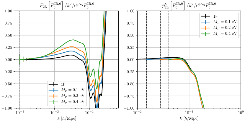
Figure 7: Subtracted two-loop and subtracted single-hard two-loop power spectrum correction over $k^{2}P_{0}(k)$. We plot the corresponding IR resummed quantities as defined in Eq. (4.47) and (4.48) below, rescaled by the two-loop growth factor power $\mathrm{e}^{6\Delta\eta}$. The three neutrino mass models computed in 2F as well as the result in 1F are shown (for simplicity we set $M_{\nu}=0.1\leavevmode\nobreak\ \mathrm{eV}$ for 1F; any difference due to neutrino mass enters there only in the input linear power spectrum). Errorbars show uncertainty from the Monte Carlo integration. The dashed vertical lines indicate the subtraction points defining the limits $b^{hh}$ (left panel) and $b^{h}$ (right panel). The double-hard subtraction points coincide for all neutrino masses, while for the single-hard limit the subtraction points left to right correspond to increasing neutrino mass.

4.2.2 Single-hard limit

Next, we consider the limit in which one of the loop momenta becomes large: $q_{1}\gg k$, $q_{2}\sim k$ (or equivalently with $q_{1}$, $q_{2}$ switched). The counterterms that renormalize this limit are one-loop diagrams with insertions of EFT operators. Computing those diagrams is rather complicated even in the 1F case, and would in the 2F scheme potentially involve further operators from the generalization of (4.17) including neutrino perturbations. Therefore we opt for the approach put forward in [71], using an ansatz for the single-hard counterterm with one extra EFT parameter.

Analogously to the one-loop case, we start by defining the two-loop integrand $\mathsf{p}_{2L}$:

$$P_{2L}(k,\eta)=\mathrm{e}^{6\Delta\eta}\int^{\Lambda}\mathop{}\!{\operator@font d}q_{1}\,q_{1}^{2}P_{0}(q)\int^{\Lambda}\mathop{}\!{\operator@font d}q_{2}\,q_{2}^{2}P_{0}(q)\int\mathop{}\!{\operator@font d}\Omega_{q_{1}}\mathop{}\!{\operator@font d}\Omega_{q_{2}}\,\mathsf{p}_{2L}(\mathbf{k},\mathbf{q}_{1},\mathbf{q}_{2};\eta)\,.$$ (4.21)

In the single-hard limit $q_{1}\to\infty$, the leading contribution comes from kernels $F^{(n)}(\dotsc,\mathbf{q}_{1},-\mathbf{q}_{1},\dotsc)\propto 1/q_{1}^{2}$. The two-loop integral can thus be factorized in this limit giving the single-hard result

$$P_{2L}^{h}(k,\eta)=2\mathrm{e}^{6\Delta\eta}\,p_{2L}^{h}(k,\eta)\,\sigma_{\mathrm{d}}^{2}\,,$$ (4.22)

where

$$p_{2L}^{h}(k,\eta)\equiv 3\int^{\Lambda}\mathop{}\!{\operator@font d}q_{2}\,q_{2}^{2}P_{0}(q)\int\frac{\mathop{}\!{\operator@font d}\Omega_{q}}{4\pi}\left(\lim_{q_{1}\to\infty}\,q_{1}^{2}\mathsf{p}_{2L}(\mathbf{k},\mathbf{q}_{1},\mathbf{q}_{2};\eta)\right)\,.$$ (4.23)

The factor $2$ in (4.22) accounts for the equivalent contribution where $q_{2}$ is hard. We compute the limit (4.23) both in the 1F and 2F schemes numerically by fixing the hard loop momentum to a large value $q_{1}\gg\Lambda$ and evaluating the resulting integral using Monte Carlo integration.

Following the prescription of [71], we assume that we can correct for the spurious UV contribution in the single-hard limit by a shift in the value of the displacement dispersion $\sigma_{\mathrm{d}}^{2}$, i.e.

$$\sigma_{\mathrm{d}}^{2}(\Lambda)\mapsto\sigma_{\mathrm{d}}^{2}(\Lambda)+\mathcal{N}\gamma_{2}(\Lambda)\,,$$ (4.24)

where the $\gamma_{2}$-term corresponds to the EFT correction and $\mathcal{N}$ is a factor introduced for convenience that we define below. The replacement yields an additional counterterm

$$2\mathrm{e}^{6\Delta\eta}\,p_{2L}^{h}(k,\eta)\,\mathcal{N}\gamma_{2}\,,$$ (4.25)

to the power spectrum. This term could in principle immediately be added to the renormalized power spectrum, however we notice that part of it is still degenerate with the double-hard limit. The definition (4.23) integrates over a hard region $q_{2}\gg k$ for external wavenumbers far below the cutoff, which yields a contribution proportional to $k^{2}P_{0}(k)$. Such a contribution is absorbed by the $\gamma_{1}$-counterterm defined above, however as discussed for the double-hard limit, we adopt a renormalization scheme where $\gamma_{1}^{2L}$ exactly cancels the double-hard region of the two-loop, now including also the double-hard contribution from the counterterm (4.25). In practice this means that we subtract the degenerate double-hard part from the single-hard contribution in analogy to the subtracted two-loop correction:

$$\bar{p}_{2L}^{h}=p_{2L}^{h}-p_{2L}^{hh}\,.$$ (4.26)

To obtain the double-hard limit $p_{2L}^{hh}$, we use the same method as for the full two-loop correction: we evaluate numerically the limit $b^{h}=\lim_{k\to 0}p_{2L}^{h}/k^{2}/P_{0}(k)$. In this limit the integral (4.23) only has support where $q_{2}\gg k$ and since $q_{1}$ is hard we recovered the double-hard limit and $p_{2L}^{hh}=b^{h}k^{2}P_{0}(k)$.

The subtracted single-hard limit $\bar{p}_{2L}^{h}$ divided by the double-hard scaling $k^{2}P_{0}(k)$ is shown in the right panel of Fig. 7 (we plot the corresponding IR resummed quantities defined in the next section). We set the cutoff to $\Lambda=1h\ \text{Mpc}^{-1}$ and the hard loop momentum to $q_{1}=10h\ \text{Mpc}^{-1}$. In the 1F scheme, the low-$k$ limit has indeed the $k^{2}P_{0}$ scaling, and we subtract the value at $k=10^{-2}h\ \text{Mpc}^{-1}$ so that the single-hard limit $\bar{p}_{2L}^{h}$ does not give a contribution degenerate with the one-loop counterterm. For the 2F scheme we also find the $k^{2}P_{0}$ scaling is approached, however for very small wavenumbers certain deviations occur. They may in part be attributed to large numerical cancellations due to our choice $q_{1}=10h\ \text{Mpc}^{-1}$, and we checked that the $k^{2}P_{0}$ scaling extends to lower $k$ for $q_{1}=5h\ \text{Mpc}^{-1}$, without changing the result within the relevant range $k\gtrsim 0.05h\ \text{Mpc}^{-1}$ where $\bar{p}_{2L}^{h}$ gives a significant contribution to the renormalized two-loop power spectrum. We therefore use a subtraction point $k\simeq 0.015,0.027,0.04h\ \text{Mpc}^{-1}$ for $M_{\nu}=0.1,0.2,0.4\leavevmode\nobreak\ \mathrm{eV}$, to read off $b^{h}$ and subtract the double-hard contribution (indicated by the vertical dashed lines in Fig. 7). As for the full two-loop correction, the definition of the double-hard subtraction point and corresponding value $b^{h}$ determines the renormalization point, hence a change of $b^{h}$ only results in a shift of $\gamma_{1}$. We check in particular that choosing $0.027h\ \text{Mpc}^{-1}$ as subtraction points also for $M_{\nu}=0.1$ and $0.4\leavevmode\nobreak\ \mathrm{eV}$ has negligible impacts on the results.

All in all, we have the two-loop counterterm

$$P_{2L}^{\mathrm{ctr}}(k,\eta;\Lambda)=2\mathrm{e}^{6\Delta\eta}\mathcal{N}\gamma_{2}(\Lambda)\,\bar{p}_{2L}^{h}(k,\eta)\,,$$ (4.27)

and the renormalized two-loop correction reads

$$P_{2L}^{\mathrm{ren}}(k,\eta;\Lambda)=\bar{P}_{2L}(k,\eta;\Lambda)+P_{2L}^{\mathrm{ctr}}(k,\eta;\Lambda)\,.$$ (4.28)

After renormalization, the CDM+baryon power spectrum at NNLO should be independent of the cutoff:

$$\frac{\mathop{}\!{\operator@font d}}{\mathop{}\!{\operator@font d}\Lambda}P_{\mathrm{NNLO}}^{\mathrm{ren}}(k,\eta;\Lambda)=0\,,$$ (4.29)

where

$$P_{\mathrm{NNLO}}^{\mathrm{ren}}(k,\eta;\Lambda)=P_{\mathrm{tree}}(k,\eta)+P_{1L}^{\mathrm{ren}}(k,\eta;\Lambda)+P_{2L}^{\mathrm{ren}}(k,\eta;\Lambda)\,.$$ (4.30)

By removing the double-hard contribution to the two-loop correction (i.e. by using the subtracted quantities $\bar{P}_{2L}$ and $\bar{p}_{2L}^{h}$), there are no degenerate UV contributions between the one- and two-loop corrections, and we can solve the RGE (4.29) independently for each term. Furthermore, the one-loop RGE (4.15) and its solution stay the same.

The remaining cutoff-dependence comes from the single-hard region of the two-loop correction, which should be corrected for by the two-loop counterterm,

$$0=\frac{\mathop{}\!{\operator@font d}}{\mathop{}\!{\operator@font d}\Lambda}\left[\bar{P}_{2L}^{h}(k,\eta;\Lambda)+P_{2L}^{\mathrm{ctr}}(k,\eta;\Lambda)\right]=2\mathrm{e}^{6\Delta\eta}\bar{p}_{2L}^{h}(k,\eta)\frac{\mathop{}\!{\operator@font d}}{\mathop{}\!{\operator@font d}\Lambda}\left[\sigma_{\mathrm{d}}^{2}(\Lambda)+\mathcal{N}\gamma_{2}(\Lambda)\right]\,,$$ (4.31)

valid at leading power in gradients. This result reflects the assumption that the single-hard region is regulated by a shift in the displacement dispersion $\sigma_{\mathrm{d}}^{2}$. The solution is

$$\gamma_{2}(\Lambda)=\overline{\gamma}_{2}+\frac{4\pi}{3\mathcal{N}}\int_{\Lambda}^{\infty}\mathop{}\!{\operator@font d}q\,P_{0}(q)\,,$$ (4.32)

where $\overline{\gamma}_{2}$ is an initial condition. We choose $\mathcal{N}=1/c$, with $c$ defined in Eq. (4.9) (and evaluated in the 2F scheme using Eq. (4.12)), in order to treat $\gamma_{1}$ and $\gamma_{2}$ on equal footing (cf. RGE for $\gamma_{1}$ (4.15)).

To check that we indeed obtain cutoff-independent loop corrections, we show the various loop and counterterm results in Fig. 8, for $M_{\nu}=0.1\leavevmode\nobreak\ \mathrm{eV}$ using two cutoffs $\Lambda=0.8$ (dashes lines) and $1h\ \text{Mpc}^{-1}$ (solid lines). The top panels show the absolute contributions, while the bottom panels show the fractional difference between the renormalized power spectra using the two cutoffs. We see that the cutoff-dependence of the renormalized one-loop correction is on the permille level up to $k\simeq 0.4h\ \text{Mpc}^{-1}$; for increasing $k$ the neglected next-to-leading gradient corrections $\mathcal{O}(k^{4}/k_{\mathrm{NL}}^{4})$ become more and more important. The double-hard limit gives the largest contribution to the bare two-loop correction, as indicated by the bare (blue) and subtracted (yellow) graphs in the right panel of Fig. 8. The single-hard limit is regulated by the counterterm (green) yielding the renormalized two-loop correction (red). We display its fractional difference using the two cutoffs in the bottom plot, where the large relative deviations at small $k$ come from the renormalized correction being very close to zero. The difference is less than 1% up to about $k=0.25h\ \text{Mpc}^{-1}$.

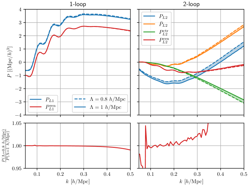
Figure 8: Cutoff-dependence of one- and two-loop corrections. Dashed and solid lines display results using $\Lambda=0.8\leavevmode\nobreak\ h/\mathrm{Mpc}$ and $\Lambda=1\leavevmode\nobreak\ h/\mathrm{Mpc}$, respectively, and the colored bands show the difference. Upper left: bare and renormalized result at one-loop. Upper right: bare, subtracted and renormalized two-loop correction, as well as the two-loop counterterm. The fractional difference between the renormalized power spectra using the two cutoffs are shown in the lower panel. The EFT parameters are set to $\gamma_{1}=\gamma_{2}=1\leavevmode\nobreak\ \mathrm{Mpc}^{2}/h^{2}$.

4.3 IR resummation

A well-known issue with the Eulerian perturbative description is that the effect of large bulk flows on the BAO peak is inadequately modelled [25, 90]. Nevertheless, this effect can relatively straightforwardly be taken into account non-perturbatively by resumming the contributions from long-wavelength displacements, known as IR resummation [27, 28, 29, 30]. We use IR resummation for both schemes 1F and 2F in order to model the BAO scales as accurately as possible.

The large bulk flows affect only the BAO wiggles and not the broadband part of the power spectrum, therefore it is useful to split the linear power spectrum into a wiggly and non-wiggly part

$$P_{0}(k)=P_{\mathrm{nw}}(k)+P_{\mathrm{w}}(k)\,.$$ (4.33)

We perform this split using the method described in [91, 92], i.e. we obtain $P_{\mathrm{nw}}$ by Fourier transforming the power spectrum to real space, removing the BAO peak, and smoothly interpolating the power spectrum without the peak. Following [30], the next step is to compute the damping factor

$$\Sigma^{2}=\frac{4\pi}{3}\mathrm{e}^{2\Delta\eta}\int_{0}^{k_{s}}\mathop{}\!{\operator@font d}q\,P_{\mathrm{nw}}(q)\left[1-j_{0}\left(\frac{q}{k_{\mathrm{osc}}}\right)+2j_{2}\left(\frac{q}{k_{\mathrm{osc}}}\right)\right]\,,$$ (4.34)

where $j_{n}$ are spherical Bessel functions, $k_{\mathrm{osc}}=h/(110\leavevmode\nobreak\ \mathrm{Mpc})$ is the wavenumber that corresponds to the BAO period and $k_{s}$ is the separation scale of long and short modes, introduced to have separate perturbative expansions in the two regimes. We use $k_{s}=0.2h\ \text{Mpc}^{-1}$, as recommended by [30]. The IR resummed power spectrum at $N$-th order is

$$P^{\mathrm{IR}}=\sum_{L=0}^{N}P_{L\text{-loop}}\left[P_{\mathrm{nw}}+P_{\mathrm{w}}\,\mathrm{e}^{-k^{2}\Sigma^{2}}\sum_{n=0}^{N-L}\frac{(k^{2}\Sigma^{2})^{n}}{n!}\right]\equiv\sum_{L=0}^{N}P_{L\text{-loop}}\left[P_{0}^{\mathrm{IR},N-L}\right]\,,$$ (4.35)

where the bracket notation $P_{L\text{-loop}}[X]$ indicates that $X$ is the linear input power spectrum that enters in the $L$-loop integrals. The exponential damping factor resums the infrared contributions, while the sum over $n$ corrects for overcounting (the IR contributions are also included perturbatively order by order in the loop evaluations) [30]. In the last equality we defined a shorthand notation for the input power spectrum in the IR resummed result $P_{0}^{\mathrm{IR},N-L}$, i.e. the quantity in the bracket, which depends on the difference $N-L$. Specifically, at the orders in perturbation theory in which we work one has

$$P_{\mathrm{LO}}^{\mathrm{IR}} =P_{\mathrm{tree}}\left[P_{\mathrm{nw}}(k)+\mathrm{e}^{-k^{2}\Sigma^{2}}P_{\mathrm{w}}(k)\right]\,,$$ (4.36)

$$P_{\mathrm{NLO}}^{\mathrm{IR}} =P_{\mathrm{tree}}\left[P_{\mathrm{nw}}(k)+\mathrm{e}^{-k^{2}\Sigma^{2}}(1+k^{2}\Sigma^{2})P_{\mathrm{w}}(k)\right]$$

$$\phantom{=}+P_{1L}\left[P_{\mathrm{nw}}(k)+\mathrm{e}^{-k^{2}\Sigma^{2}}P_{\mathrm{w}}(k)\right]\,,$$ (4.37)

$$P_{\mathrm{NNLO}}^{\mathrm{IR}} =P_{\mathrm{tree}}\left[P_{\mathrm{nw}}(k)+\mathrm{e}^{-k^{2}\Sigma^{2}}\left(1+k^{2}\Sigma^{2}+\frac{1}{2}(k^{2}\Sigma^{2})^{2}\right)P_{w}(k)\right]$$

$$\phantom{=}+P_{1L}\left[P_{\mathrm{nw}}(k)+\mathrm{e}^{-k^{2}\Sigma^{2}}(1+k^{2}\Sigma^{2})P_{\mathrm{w}}(k)\right]$$

$$\phantom{=}+P_{2L}\left[P_{\mathrm{nw}}(k)+\mathrm{e}^{-k^{2}\Sigma^{2}}P_{\mathrm{w}}(k)\right]\,.$$ (4.38)

Note that the tree-level power spectrum is non-trivial in the 2F scheme and given by

$$P_{\mathrm{tree}}\left[P_{0}\right](k,\eta)=\left[F^{(1)}(k,\eta)\right]^{2}P_{0}(k)\,.$$ (4.39)

In deriving Eq. (4.35) in the Eulerian theory, the following property of the kernels in the soft limit is key [30]:

$$F^{(n)}(\mathbf{q}_{1},\dotsc,\mathbf{q}_{n})\to\frac{m!}{n!}F^{(m)}(\mathbf{q}_{1},\dotsc,\mathbf{q}_{m})\frac{\mathbf{q}\cdot\mathbf{q}_{m+1}}{q_{m+1}^{2}}\dotsb\frac{\mathbf{q}\cdot\mathbf{q}_{n}}{q_{n}^{2}}$$ (4.40)

in the limit where $q_{1},\dotsc,q_{m}$ are much smaller than the remaining arguments $q_{m+1},\dotsc,q_{n}$ and where $\mathbf{q}=\sum\mathbf{q}_{i}$. This factorization follows from Galilean invariance [93], which is certainly also a symmetry in the 2F scheme. Therefore the IR resummed equation (4.35) is valid also in the 2F case.

In practice, we use the following simplified expression to evaluate IR resummed loops

$$P_{L\text{-loop}}\left[P_{\mathrm{nw}}+P_{\mathrm{w}}\,\mathrm{e}^{-k^{2}\Sigma^{2}}\sum_{n=0}^{N-L}\frac{(k^{2}\Sigma^{2})^{n}}{n!}\right]\\ \to P_{L\text{-loop}}\left[P_{\mathrm{nw}}\right]+\left(P_{L\text{-loop}}\left[P_{\mathrm{nw}}+P_{\mathrm{w}}\right]-P_{L\text{-loop}}\left[P_{\mathrm{nw}}\right]\right)\times\mathrm{e}^{-k^{2}\Sigma^{2}}\sum_{n=0}^{N-L}\frac{(k^{2}\Sigma^{2})^{n}}{n!}\,,$$ (4.41)

which is valid up to corrections of $\mathcal{O}(P_{\mathrm{w}}^{2})$ as well as diagrams involving $P_{\mathrm{w}}$ inside a hard loop. Neglecting these corrections is a good approximation because $P_{\mathrm{w}}$ is small compared to $P_{\mathrm{nw}}$, and it oscillates around zero so that its integral vanishes.

4.4 All together: summary

We end this section by writing down the final expressions for the power spectrum up to NNLO including both IR resummation and EFT corrections. We have

$$P_{\mathrm{LO}}^{\mathrm{IR}}(k) =P_{\mathrm{tree}}\left[P_{0}^{\mathrm{IR},0}\right]\,,$$ (4.42)

$$P_{\mathrm{NLO}}^{\mathrm{IR}}(k) =P_{\mathrm{tree}}\left[P_{0}^{\mathrm{IR},1}\right]+P_{1L}\left[P_{0}^{\mathrm{IR},0}\right]+P_{1L}^{\mathrm{ctr}}\left[P_{0}^{\mathrm{IR},0}\right]\,,$$ (4.43)

$$P_{\mathrm{NNLO}}^{\mathrm{IR}}(k) =P_{\mathrm{tree}}\left[P_{0}^{\mathrm{IR},2}\right]+P_{1L}\left[P_{0}^{\mathrm{IR},1}\right]+P_{1L}^{\mathrm{ctr}}\left[P_{0}^{\mathrm{IR},1}\right]+\bar{P}_{2L}\left[P_{0}^{\mathrm{IR},0}\right]+P_{2L}^{\mathrm{ctr}}\left[P_{0}^{\mathrm{IR},0}\right]\,,$$ (4.44)

where the counterterms are given by

$$P_{1L}^{\mathrm{ctr}}\left[P_{0}^{\mathrm{IR},N-L}\right](k,\eta;\Lambda) =-2\mathrm{e}^{4\Delta\eta}\,\gamma_{1}(\Lambda)k^{2}P_{0}^{\mathrm{IR},N-L}(k)\,,$$ (4.45)

$$P_{2L}^{\mathrm{ctr}}\left[P_{0}^{\mathrm{IR},N-L}\right](k,\eta;\Lambda) =2\frac{\mathrm{e}^{6\Delta\eta}}{c(\eta)}\gamma_{2}(\Lambda)\,\bar{p}_{2L}^{h}\left[P_{0}^{\mathrm{IR},N-L}\right](k,\eta;\Lambda)\,,$$ (4.46)

with $c$ defined in Eq. (4.9) and the subtracted quantities defined as

$$\bar{P}_{2L}\left[P_{0}^{\mathrm{IR},N-L}\right](k,\eta;\Lambda) =P_{2L}\left[P_{0}^{\mathrm{IR},N-L}\right](k,\eta;\Lambda)-b^{hh}k^{2}P_{0}^{\mathrm{IR},N-L}(k)\,,$$ (4.47)

$$\bar{p}_{2L}^{h}\left[P_{0}^{\mathrm{IR},N-L}\right](k,\eta;\Lambda) =\bar{p}_{2L}^{h}\left[P_{0}^{\mathrm{IR},N-L}\right](k,\eta;\Lambda)-b^{h}k^{2}P_{0}^{\mathrm{IR},N-L}(k)\,.$$ (4.48)

The single-hard contribution $p_{2L}^{h}$ was defined in Eq. (4.23) and the RGEs for the EFT parameters were given in Eqs. (4.15) and (4.31). The double-hard limit constants $b^{hh}$ and $b^{h}$ are computed in the same way as in subsections 4.2.1 and 4.2.2, but using $P_{0}^{\mathrm{IR},N-L}$ as the linear power spectrum, e.g $b^{hh}=\lim_{k\to 0}P_{2L}\left[P_{0}^{\mathrm{IR},N-2}\right]/k^{2}/P_{0}^{\mathrm{IR},N-2}$. In general, the EFT discussion in subsections 4.1 and 4.2 above can immediately be promoted to include IR resummation by the replacement $P_{0}\to P_{0}^{\mathrm{IR},N-L}$.

For completeness, we note again that in the 1F scheme the time-dependence is factored out, so to obtain the power spectrum at $z=0$ we can use $\eta_{\mathrm{ini}}=0$ and $\Delta\eta=0$. In the 2F scheme on the other hand, we chose the matching between the Boltzmann hierarchy and the two-fluid description at $\eta_{\mathrm{ini}}$ corresponding to $z=25$. Therefore, to obtain the quantities $P_{0}^{\mathrm{IR},N-L}$, we take the linear power spectrum from CLASS at $z=0$ or $z=25$ depending on the scheme, split it into its wiggly and non-wiggly components, compute the damping factor $\Sigma^{2}$ and use the definition in Eq. (4.35).

5 Comparison to N-body simulations

To calibrate the EFT parameters and perform a comparison of the 1F and 2F schemes in the effective theory, we utilise the Quijote N-body simulations [72]. In particular, we use the set of massive neutrinos simulations with $512^{3}$ CDM particles and $512^{3}$ neutrino particles in a cubic box of size $(1\leavevmode\nobreak\ \mathrm{Gpc}/h)^{3}$. Moreover, we use the simulations with pair fixed initial conditions that significantly reduce the cosmic variance for the power spectrum. The cosmological parameters are $\Omega_{m}=0.3175$, $\Omega_{b}=0.049$, $h=0.6711$, $n_{s}=0.9624$, $\sigma_{8}=0.834$ and the neutrinos mass is $M_{\nu}=0.1$, $0.2$ and $0.4\leavevmode\nobreak\ \mathrm{eV}$ in the different models respectively. We estimate the power spectrum and uncertainty at $z=0$ using the average and standard deviation of the 500 realizations.

On the largest scales, the binning method used to obtain the power spectrum from the simulations become significant and has to be taken into account when comparing simulation and theory. We use the Pylians library to perform the same binning on the linear power spectrum. Instead of binning also the loop corrections, we can equivalently compare the theoretical results to the “unbinned” N-body power spectrum

$$P_{\mathrm{data}}(k)=\frac{P_{0}(k,z=0)}{P_{0}^{\mathrm{binned}}(k,z=0)}P_{\mathrm{data}}^{\mathrm{binned}}(k)\,.$$ (5.1)

The EFT parameters are calibrated by minimizing the following $\chi^{2}$ at NLO and NNLO:

$$\chi_{\mathrm{NLO}}^{2} =\sum_{k=k_{\mathrm{min}}}^{k_{\mathrm{max}}}\frac{\left[P_{\mathrm{data}}(k)-P_{\mathrm{NLO}}^{\mathrm{IR}}(k,\gamma_{1})\right]^{2}}{\left[\Delta P_{\mathrm{data}}(k)\right]^{2}}\,,$$ (5.2)

$$\chi_{\mathrm{NNLO}}^{2} =\sum_{k=k_{\mathrm{min}}}^{k_{\mathrm{max}}}\frac{\left[P_{\mathrm{data}}(k)-P_{\mathrm{NNLO}}^{\mathrm{IR}}(k,\gamma_{1},\gamma_{2})\right]^{2}}{\left[\Delta P_{\mathrm{data}}(k)\right]^{2}}\,,$$ (5.3)

where $\Delta P_{\mathrm{data}}(k)$ is the estimated uncertainty of the N-body power spectrum. We have $k_{\mathrm{min}}=0.0089h\ \text{Mpc}^{-1}$ and at $k_{\mathrm{max}}=0.1$ and $0.3h\ \text{Mpc}^{-1}$ we have 14 and 46 wavenumber grid points in the sum, respectively. The perturbative results $P_{\mathrm{NLO}}^{\mathrm{IR}}$ and $P_{\mathrm{NNLO}}^{\mathrm{IR}}$ are calculated using Eqs. (4.43) and (4.44) with cutoff $\Lambda=1h\ \text{Mpc}^{-1}$ and where the hard limits are evaluated by fixing the hard momenta to $q_{1}=10h\ \text{Mpc}^{-1}$ as described in the previous section.

We consider the following cases

NLO $$\{\bar{\gamma}_{1}\}$$ one-loop, 1-parameter,

$$\text{NLO},\leavevmode\nobreak\ \bar{\gamma}_{1}=\bar{\gamma}_{1}^{\text{[NNLO]}} \{\emptyset\} \text{one-loop, 0-parameter with }\bar{\gamma}_{1}\text{ fixed from NNLO fit,}$$

$$\text{NNLO},\bar{\gamma}_{2}=\bar{\gamma}_{1} \{\bar{\gamma}_{1}\} \text{two-loop, 1-parameter with }\bar{\gamma}_{2}=\bar{\gamma}_{1}\,,$$

NNLO $$\{\bar{\gamma}_{1},\bar{\gamma}_{2}\}$$ two-loop, 2-parameter,

where the NLO cases are fit using Eq. (5.2) and NNLO cases using Eq. (5.3). We calibrate the EFT parameters in the limit $\Lambda\to\infty$ (cf. Eqs. (4.16) and (4.32)). The second case, NLO $\bar{\gamma}_{1}=\bar{\gamma}_{1}^{\text{[NNLO]}}$, is not fitted since $\bar{\gamma}_{1}$ is fixed from the two-parameter NNLO case. We explain the motivation for this case below. The third case, NNLO $\bar{\gamma}_{2}=\bar{\gamma}_{1}$, is motivated by the assumption that in the EFT, the displacement dispersion is corrected in an universal manner as $\sigma_{\mathrm{d}}^{2}\to\sigma_{\mathrm{d}}^{2}+\gamma_{1}/c$ both at one- and two-loop.

5.1 Results

We begin by comparing the full 2F solution for the various NLO/NNLO calibration cases above with the most phenomenologically relevant neutrino mass $M_{\nu}=0.1\leavevmode\nobreak\ \mathrm{eV}$. In Fig. 9 we show the power spectrum using three pivot scales $k_{\mathrm{max}}=0.103$, $0.148$ and $0.204h\ \text{Mpc}^{-1}$, normalized to the N-body results. The gray band indicates estimated uncertainty from the N-body simulation and the red shading corresponds to an ansatz for the expected theoretical uncertainty at NLO (light shading) and NNLO (darker shading) [94]. In all panels, there is a “bump” feature in the relative difference around $k=0.01$ – $0.05h\ \text{Mpc}^{-1}$ of a few permille (i.e. well within the uncertainty of the N-body data) that arises due to finite N-body box size and binning uncertainty not captured by the correction (5.1). Nevertheless, all cases can be fitted to lie within the N-body uncertainty up to even the largest pivot scale. Depending on the loop order, we are subject to overfitting above a certain $k_{\mathrm{max}}$. In particular, given the expected theoretical uncertainties, we see that the NLO result differs much less from N-body beyond $k\simeq 0.10h\ \text{Mpc}^{-1}$ than expected from the missing two-loop correction, and similarly the NNLO result remains in good agreement above $k\simeq 0.10h\ \text{Mpc}^{-1}$, indicating overfitting. Ideally, we would be able to calibrate the EFT parameters precisely below $k=0.05h\ \text{Mpc}^{-1}$ where the perturbative uncertainty is small, but in practice the moderate simulation uncertainty (even after cosmic variance is reduced), a small number of grid points and finite box size effects complicates the picture.

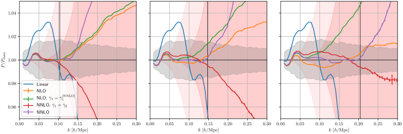
Figure 9: CDM+baryon power spectrum computed in the 2F scheme normalized to N-body data. We show the perturbative results at NLO and NNLO with different assumptions on the EFT parameters, for pivot scales $k_{\mathrm{max}}=0.103$ (left) $0.148$ (middle) and $0.204h\ \text{Mpc}^{-1}$ (right). The gray band indicates the N-body uncertainty, while the red shaded area display estimated theoretical uncertainty at one-loop (light shading) and two-loop (darker shading). The sum of neutrino masses is $M_{\nu}=0.1\leavevmode\nobreak\ \mathrm{eV}$.

To gauge the extent of overfitting at NLO, we introduce a 0-parameter NLO case where the $\gamma_{1}$ parameter is fixed to that in the NNLO case with the same pivot scale. At NNLO, there is a larger window in which the theoretical uncertainty is still small and hence more data points to measure $\gamma_{1}$ precisely. Moreover, in our renormalization scheme $\gamma_{1}$ remains the same after adding the two-loop correction, up to numerical uncertainty and overfitting. Therefore, the degree of overfitting is reduced in the NLO $\bar{\gamma}_{1}=\bar{\gamma}_{1}^{\text{[NNLO]}}$ case.

The $\chi^{2}$ per degree of freedom (d.o.f.) is shown for the different fits in Fig. 10. Since we are ultimately interested in assessing the effect of non-linear neutrino perturbations on the power spectrum, i.e. comparing the performance of the 1F and 2F schemes, we chose a simple estimator for the N-body uncertainty, for example not taking into account correlations between different bins. This is reflected by the small $\chi^{2}/\mathrm{d.o.f.}\ll 1$. We find that the $\bar{\gamma}_{1}=\bar{\gamma}_{2}$ ansatz at NNLO proposed by [71] does not work as well when including the exact time-dependence and effect of neutrinos, and even performs worse than the NLO case at $k\simeq 0.12h\ \text{Mpc}^{-1}$.

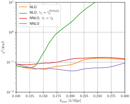
Figure 10: Reduced $\chi^{2}$ for the various calibration cases at NLO and NNLO as a function of the pivot scale $k_{\mathrm{max}}$.

The best-fit EFT parameters $\bar{\gamma}_{1}$ and $\bar{\gamma}_{2}$ as a function of $k_{\mathrm{max}}$ are displayed in Fig. 11. We show the results from both schemes 1F and 2F, indicating $1\sigma$ uncertainty in the shaded bands. At NLO, we find that the $\bar{\gamma}_{1}$ measurement is consistent with a constant up to about $k_{\mathrm{max}}\simeq 0.11h\ \text{Mpc}^{-1}$ where the parameter starts exhibiting a running. At NNLO (with both parameters varied), this plateau for $\bar{\gamma}_{1}$ extends to $k_{\mathrm{max}}\simeq 0.14h\ \text{Mpc}^{-1}$, and the measurement within $1\sigma$ is consistent with a constant up to around $0.2h\ \text{Mpc}^{-1}$. The $\bar{\gamma}_{2}$ parameter (rightmost panel) can only be constrained beyond $k_{\mathrm{max}}\simeq 0.15h\ \text{Mpc}^{-1}$, because the two-loop counterterm (i.e. the subtracted single-hard limit (4.27)) is exceedingly small for lower wavenumbers. We find that when both parameters are allowed to vary at NNLO, they assume different values, giving another confirmation that the NNLO 1-parameter $\bar{\gamma}_{1}=\bar{\gamma}_{2}$ model cannot match the data with the same accuracy. In the second leftmost plot we show the best-fit parameter in this model. It features a considerable running compared to the other cases even at low $k_{\mathrm{max}}\simeq 0.1h\ \text{Mpc}^{-1}$, suggesting a degree of overfitting already from large scales. Before commenting on the difference in the calibrated EFT parameters in the 1F and 2F schemes as is seen in Fig. 11, we discuss the power spectrum and $\chi^{2}$ in the two schemes.

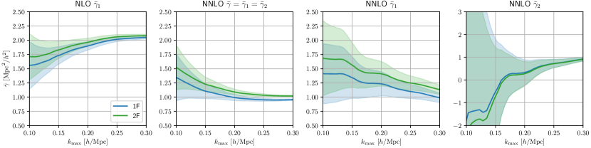
Figure 11: Measured parameters $\gamma_{1}$, $\gamma_{2}$ and $\gamma=\gamma_{1}=\gamma_{2}$ as a function of $k_{\mathrm{max}}$. We show the results from the 1F scheme (blue) and 2F scheme (green) for a neutrino mass sum $M_{\nu}=0.1\leavevmode\nobreak\ \mathrm{eV}$. The shaded regions indicate $1\sigma$ uncertainty.

Next, we compare the 1F and 2F schemes for $M_{\nu}=0.1\leavevmode\nobreak\ \mathrm{eV}$. We find similar conclusions for the other neutrino mass cosmologies. The power spectra for the two schemes are shown in Fig. 12, using $k_{\mathrm{max}}=0.15h\ \text{Mpc}^{-1}$, and the $\chi^{2}/\mathrm{d.o.f.}$ as a function of the pivot scale is shown in the left panel of Fig. 13. We find that both schemes can broadly model the data equally accurately, with some minimal differences. This suggests that the difference between the schemes for the bare density power spectrum (arising mostly due to relaxing the EdS approximation, see Fig. 3 and discussion in Sec. 3) can to large extent be absorbed into the counterterms. In particular, the difference can be captured by the $k^{2}P_{0}$-counterterm leading to a shift in the value $\bar{\gamma}_{1}$. This is exactly what we see in Fig. 11. Both in the NLO and NNLO cases, we have an approximate shift $\Delta\bar{\gamma}_{1}\approx-0.2\leavevmode\nobreak\ \mathrm{Mpc}^{2}/h^{2}$ between the 1F and 2F schemes. The shift is consistent with the findings of [39] for the one-loop bispectrum with the EdS approximation relaxed. Furthermore, we find that the two-loop EFT parameter $\bar{\gamma}_{2}$ is unchanged in the 2F scheme as compared to 1F, as seen for $k_{\mathrm{max}}>0.15h\ \text{Mpc}^{-1}$ in the rightmost panel of Fig. 11.

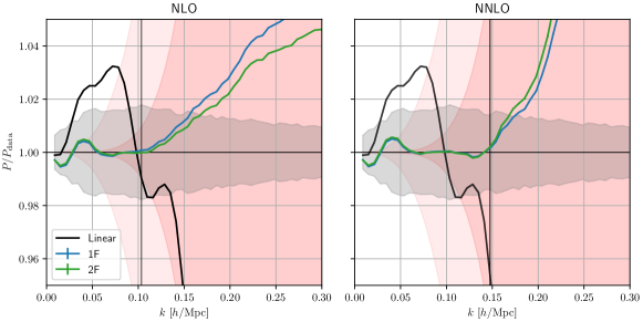
Figure 12: CDM+baryon power spectrum at NLO (left) and NNLO (right) in the 1F (blue) and 2F (green) schemes, normalized to the N-body result. The gray band indicates the N-body uncertainty, while the red shaded area display estimated theoretical uncertainty at one-loop (light shading) and two-loop (darker shading). The pivot scale is $k_{\mathrm{max}}=0.148h\ \text{Mpc}^{-1}$ and the sum of neutrino masses is $M_{\nu}=0.1\leavevmode\nobreak\ \mathrm{eV}$.

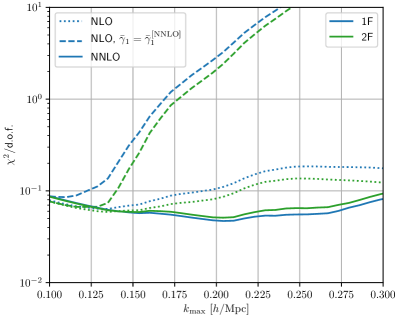
Figure 13: Left: Reduced $\chi^{2}$ as a function of $k_{\mathrm{max}}$ for the 1F and 2F schemes, at NLO (1- and 0-parameter) and NNLO (2-parameter) in perturbation theory. Right: Reduced $\chi^{2}$ for different neutrino masses, computed in the 2F scheme at NNLO (2-parameter fit).

Finally, we consider the three cosmologies with $M_{\nu}=0.1$, $0.2$ and $0.4\leavevmode\nobreak\ \mathrm{eV}$, computed at NNLO (2-parameter) in the full 2F solution. The reduced $\chi^{2}$ for the different models is displayed in the right panel of Fig. 13. By accident, the “bump” feature from finite box effects is slightly smaller for $M_{\nu}=0.2\leavevmode\nobreak\ \mathrm{eV}$ than the other neutrino masses, leading to a smaller $\chi^{2}$ for low $k_{\mathrm{max}}$. Moreover, for $M_{\nu}=0.4\leavevmode\nobreak\ \mathrm{eV}$, the linear 2F solution is off by almost a percent for $k<0.01h\ \text{Mpc}^{-1}$ (see Fig. 2), yielding a slightly larger $\chi^{2}$ around $k_{\mathrm{min}}$. Apart from these insignificant discrepancies, we find that all neutrino models can match the N-body results accurately using the 2F scheme. This is also seen from the power spectra plots in Fig. 1.

The best-fit EFT parameters for the different neutrino mass models are shown in Fig. 14. In the left plot we use the 1-parameter NLO approach while in the middle and right plots we show the NNLO 2-parameter model. It is not surprising that the parameters acquire different values for the different cosmologies: the part of the counterterms correcting for the inaccuracy of SPT is altered due to different values of the displacement dispersion $\sigma_{\mathrm{d}}^{2}$ and the $c$-coefficient, and the part accounting for the impact of actual short-scale physics changes due to the impact of massive neutrinos on strongly non-linear scales. At NNLO, we measure a shift $\Delta\bar{\gamma}_{1}\simeq-0.14\leavevmode\nobreak\ \mathrm{Mpc}^{2}/h^{2}$ at $k_{\mathrm{max}}=0.14h\ \text{Mpc}^{-1}$ and $\Delta\bar{\gamma}_{2}\simeq-0.2\leavevmode\nobreak\ \mathrm{Mpc}^{2}/h^{2}$ at $k_{\mathrm{max}}=0.17h\ \text{Mpc}^{-1}$ when doubling the sum of neutrino masses. We quote the value of the $c$-coefficient as well as the measured EFT parameters $\gamma_{1}(\Lambda)$ and $\gamma_{2}(\Lambda)$ for $\Lambda=1h\ \text{Mpc}^{-1}$ and $\Lambda\to\infty$ for the different neutrino cosmologies in Tab. 2.

Figure 14: Measured parameters $\bar{\gamma}_{1}$, $\bar{\gamma}_{2}$ and as a function of $k_{\mathrm{max}}$ for the different cosmologies with $M_{\nu}=0.1$, $0.2$ and $0.4\leavevmode\nobreak\ \mathrm{eV}$. The shaded regions indicate $1\sigma$ uncertainty.

Table 2: Measured EFT parameters and constant $c$ for different neutrino masses with cutoff $\Lambda=1h\ \text{Mpc}^{-1}$ and pivot scale $k_{\mathrm{pivot}}=0.15h\ \text{Mpc}^{-1}$.

	$c$	$\gamma_{1}(\Lambda)$	$\bar{\gamma}_{1}$	$\gamma_{2}(\Lambda)$	$\bar{\gamma_{2}}$
$M_{\nu}=0.1\leavevmode\nobreak\ \mathrm{eV}$	$0.269$	$1.81\pm 0.41$	$1.58\pm 0.41$	$-0.62\pm 2.4$	$-0.85\pm 2.4$
$M_{\nu}=0.2\leavevmode\nobreak\ \mathrm{eV}$	$0.254$	$1.71\pm 0.42$	$1.48\pm 0.42$	$-0.072\pm 2.3$	$-0.3\pm 2.3$
$M_{\nu}=0.4\leavevmode\nobreak\ \mathrm{eV}$	$0.228$	$1.61\pm 0.39$	$1.4\pm 0.39$	$0.46\pm 2.1$	$0.25\pm 2.1$

In summary, we can accurately match the Quijote N-body data both at NLO and NNLO using the full 2F solution, however being subject to a certain degree of overfitting. The window where the EFT parameters can be precisely measured is relatively small and involve uncertainties from the N-body simulation. We compared the 1F and 2F schemes and found that the difference of the unrenormalized power spectrum can largely be absorbed in the one-loop counterterm, leading to a shift in the EFT parameter $\bar{\gamma}_{1}$.

6 Conclusions

In this work we have performed a precision calculation of the CDM+baryon density and velocity power spectrum at next-to-next-to-leading (two-loop) order taking the full time- and scale-dependence of neutrino perturbations beyond the linear level as well as exact $\Lambda$CDM ($+M_{\nu}$) time-dependence into account. Our aim is to assess the accuracy of the commonly used approach in which the aforementioned effects are neglected.

To describe the impact of neutrinos in gravitational collapse, we use a hybrid two-component fluid scheme introduced in [61] and further developed in [57]. The idea is that neutrinos can only be described by a fluid well after they have become non-relativistic, because the lower and higher order multipoles effectively decouple by powers of $T_{\nu}/m_{\nu}$. Therefore, we can use the full, linear Boltzmann hierarchy until an intermediate redshift $z=25$, where we map the equations onto a two-component fluid consisting of CDM+baryons (one joint component) and neutrinos. The large neutrino free-streaming is reflected in an effective neutrino sound velocity, which we compute from linear theory. The two-component fluid system can readily be realized in the framework for computing loop corrections in cosmologies with general time- and scale-dependence introduced in [57].

We compare the (unrenormalized) two-loop CDM+baryon density and velocity power spectra at $z=0$ from the full solution including neutrino perturbations beyond the linear level and exact time-dependence (2F scheme) to the commonly used simplified treatment with only linear neutrino perturbations and EdS dynamics for CDM+baryons (1F scheme). For the density spectrum, the main difference arises due to the departure from EdS, leading to 0.7% deviation at $k=0.15h\ \text{Mpc}^{-1}$ (consistent with the results in [57]), approximately neutrino mass independent. On the other hand, for the velocity spectrum, the deviation in the 1F scheme is neutrino mass dependent; for the largest neutrino mass $M_{\nu}=0.4\leavevmode\nobreak\ \mathrm{eV}$ the deviation is larger than a percent for $k\gtrsim 0.08h\ \text{Mpc}^{-1}$. For $k=0.15h\ \text{Mpc}^{-1}$ the deviation in the velocity or cross power spectra up to two-loop are $2.7\%,1.3\%,0.8\%$ for $M_{\nu}=0.4,0.2,0.1\leavevmode\nobreak\ \mathrm{eV}$, respectively, and even somewhat larger, $2.7\%,2.0\%,1.6\%$, when going only up to one-loop, due to a partial cancellation between one- and two-loop terms. Therefore, the commonly used 1F approximation is questionable for the velocity spectra when aiming at percent accuracy, implying that the 2F scheme should be used to access the neutrino mass sensitivity in redshift space.

Furthermore, we check to what extent the two-loop power spectrum on mildly non-linear scales in the presence of free-streaming massive neutrinos can be reproduced by a massless model by adjusting the overall amplitude of fluctuations. We find that the massless model can reproduce the total matter density power spectrum of the smallest neutrino mass to within a percent, but for the larger neutrino masses the neutrino free-streaming scale $k_{\mathrm{FS}}$ is larger and mimicking the power spectrum in the massless model is more challenging.

To assess the performance of the full 2F solution and the simpler 1F scheme as accurately as possible, and to compare to N-body data, we take into account EFT corrections as well as effects of large bulk flows from the IR. We find that the $k^{2}$ scaling of the kernels – expected from momentum conservation in the limit when the external wavenumber $k$ goes to zero (or the other momenta go to infinity) – is slightly spoiled by the free-streaming scale, but recovered when $k\ll k_{\mathrm{FS}}$ or $k\gg k_{\mathrm{FS}}$. Therefore, we assume a large scale separation $k_{\mathrm{FS}}\ll k\ll q$, where $q$ is the scale of hard loop momenta, when analysing the UV limit of the 2F model. This assumption is appropriate for the smallest neutrino masses, but breaks down for the largest neutrino mass. At one-loop, we show that the usual $k^{2}P_{0}(k)$ counterterm absorbs the cutoff-dependence. The double-hard region of the two-loop contribution can also be corrected by this counterterm. For the single-hard region, we employ a numerical treatment yielding a counterterm that exactly captures the scale-dependence of the UV-limit of SPT, with one extra EFT parameter.

We compare the perturbative results of both the 1F and 2F schemes to N-body data, at different orders in perturbation theory and with various number of free parameters. The power spectrum in the 2F scheme matches the N-body data within a percent up to $k\simeq 0.12h\ \text{Mpc}^{-1}$ and $k\simeq 0.16h\ \text{Mpc}^{-1}$ for NLO and NNLO, respectively, using a pivot scale $k_{\mathrm{max}}=0.148h\ \text{Mpc}^{-1}$. We find that the 1F scheme can achieve similar accuracy, indicating that the deviation in the bare power spectrum can be absorbed by the counterterms. In particular, the main source of error in the 1F density power spectrum comes from the EdS approximation, and it is largely degenerate with the one-loop counterterm. We measure a shift in the EFT parameter $\Delta\bar{\gamma}_{1}=-0.2\leavevmode\nobreak\ \mathrm{Mpc}^{2}/h^{2}$ between the 1F and 2F schemes that accounts for the discrepancy.

In total, we have scrutinized the effect of massive neutrino perturbations taking into account the full impact of time- and scale-dependent growth on non-linear kernels for CDM+baryon as well as neutrino density and velocity. We further capture the exact time-dependence of $\Lambda$CDM ($+M_{\nu}$). The impact on the two-loop density power spectrum is to great extent degenerate with counterterms. The influence of time- and scale-dependent growth due to massive neutrinos is larger on the velocity spectrum, suggesting that the full 2F treatment for neutrinos is warranted to access the neutrino mass information encoded in redshift space distortions. This motivates an analysis of the power spectrum in redshift space within the 2F scheme, which we leave to future work.

References

- [1] SPT collaboration, Cluster Cosmology Constraints from the 2500 deg2 SPT-SZ Survey: Inclusion of Weak Gravitational Lensing Data from Magellan and the Hubble Space Telescope, Astrophys. J. 878 (2019) 55 [1812.01679].
- [2] DES collaboration, Dark Energy Survey year 1 results: Cosmological constraints from galaxy clustering and weak lensing, Phys. Rev. D 98 (2018) 043526 [1708.01530].
- [3] eBOSS collaboration, Completed SDSS-IV extended Baryon Oscillation Spectroscopic Survey: Cosmological implications from two decades of spectroscopic surveys at the Apache Point Observatory, Phys. Rev. D 103 (2021) 083533 [2007.08991].
- [4] PFS Team collaboration, Extragalactic science, cosmology, and Galactic archaeology with the Subaru Prime Focus Spectrograph, Publ. Astron. Soc. Jap. 66 (2014) R1 [1206.0737].
- [5] Euclid Theory Working Group collaboration, Cosmology and fundamental physics with the Euclid satellite, Living Rev. Rel. 16 (2013) 6 [1206.1225].
- [6] LSST Science, LSST Project collaboration, LSST Science Book, Version 2.0, 0912.0201.
- [7] DESI collaboration, The Dark Energy Spectroscopic Instrument (DESI), 1907.10688.
- [8] T. Eifler et al., Cosmology with the Roman Space Telescope – multiprobe strategies, Mon. Not. Roy. Astron. Soc. 507 (2021) 1746 [2004.05271].
- [9] J. Lesgourgues and S. Pastor, Massive neutrinos and cosmology, Phys. Rept. 429 (2006) 307 [astro-ph/0603494].
- [10] B. Audren, J. Lesgourgues, S. Bird, M. G. Haehnelt and M. Viel, Neutrino masses and cosmological parameters from a Euclid-like survey: Markov Chain Monte Carlo forecasts including theoretical errors, JCAP 01 (2013) 026 [1210.2194].
- [11] L. Amendola et al., Cosmology and fundamental physics with the Euclid satellite, Living Rev. Rel. 21 (2018) 2 [1606.00180].
- [12] A. Boyle and E. Komatsu, Deconstructing the neutrino mass constraint from galaxy redshift surveys, JCAP 03 (2018) 035 [1712.01857].
- [13] S. Mishra-Sharma, D. Alonso and J. Dunkley, Neutrino masses and beyond- CDM cosmology with LSST and future CMB experiments, Phys. Rev. D 97 (2018) 123544 [1803.07561].
- [14] T. Sprenger, M. Archidiacono, T. Brinckmann, S. Clesse and J. Lesgourgues, Cosmology in the era of Euclid and the Square Kilometre Array, JCAP 02 (2019) 047 [1801.08331].
- [15] T. Brinckmann, D. C. Hooper, M. Archidiacono, J. Lesgourgues and T. Sprenger, The promising future of a robust cosmological neutrino mass measurement, JCAP 01 (2019) 059 [1808.05955].
- [16] A. Chudaykin and M. M. Ivanov, Measuring neutrino masses with large-scale structure: Euclid forecast with controlled theoretical error, JCAP 11 (2019) 034 [1907.06666].
- [17] C. Hahn, F. Villaescusa-Navarro, E. Castorina and R. Scoccimarro, Constraining with the bispectrum. Part I. Breaking parameter degeneracies, JCAP 03 (2020) 040 [1909.11107].
- [18] W. L. Xu, N. DePorzio, J. B. Muñoz and C. Dvorkin, Accurately Weighing Neutrinos with Cosmological Surveys, Phys. Rev. D 103 (2021) 023503 [2006.09395].
- [19] A. Boyle and F. Schmidt, Neutrino mass constraints beyond linear order: cosmology dependence and systematic biases, JCAP 04 (2021) 022 [2011.10594].
- [20] F. Bernardeau, S. Colombi, E. Gaztanaga and R. Scoccimarro, Large scale structure of the universe and cosmological perturbation theory, Phys. Rept. 367 (2002) 1 [astro-ph/0112551].
- [21] M. Crocce and R. Scoccimarro, Renormalized cosmological perturbation theory, Phys. Rev. D 73 (2006) 063519 [astro-ph/0509418].
- [22] D. Baumann, A. Nicolis, L. Senatore and M. Zaldarriaga, Cosmological Non-Linearities as an Effective Fluid, JCAP 07 (2012) 051 [1004.2488].
- [23] J. J. M. Carrasco, M. P. Hertzberg and L. Senatore, The Effective Field Theory of Cosmological Large Scale Structures, JHEP 09 (2012) 082 [1206.2926].
- [24] V. Desjacques, D. Jeong and F. Schmidt, Large-Scale Galaxy Bias, Phys. Rept. 733 (2018) 1 [1611.09787].
- [25] D. J. Eisenstein, H.-j. Seo and M. J. White, On the Robustness of the Acoustic Scale in the Low-Redshift Clustering of Matter, Astrophys. J. 664 (2007) 660 [astro-ph/0604361].
- [26] H.-J. Seo and D. J. Eisenstein, Improved forecasts for the baryon acoustic oscillations and cosmological distance scale, Astrophys. J. 665 (2007) 14 [astro-ph/0701079].
- [27] L. Senatore and M. Zaldarriaga, The IR-resummed Effective Field Theory of Large Scale Structures, JCAP 02 (2015) 013 [1404.5954].
- [28] T. Baldauf, M. Mirbabayi, M. Simonović and M. Zaldarriaga, Equivalence Principle and the Baryon Acoustic Peak, Phys. Rev. D 92 (2015) 043514 [1504.04366].
- [29] Z. Vlah, U. Seljak, M. Y. Chu and Y. Feng, Perturbation theory, effective field theory, and oscillations in the power spectrum, JCAP 03 (2016) 057 [1509.02120].
- [30] D. Blas, M. Garny, M. M. Ivanov and S. Sibiryakov, Time-Sliced Perturbation Theory II: Baryon Acoustic Oscillations and Infrared Resummation, JCAP 07 (2016) 028 [1605.02149].
- [31] R. Scoccimarro, H. M. P. Couchman and J. A. Frieman, The Bispectrum as a Signature of Gravitational Instability in Redshift-Space, Astrophys. J. 517 (1999) 531 [astro-ph/9808305].
- [32] R. Scoccimarro, Redshift-space distortions, pairwise velocities and nonlinearities, Phys. Rev. D 70 (2004) 083007 [astro-ph/0407214].
- [33] Z. Vlah, U. Seljak, P. McDonald, T. Okumura and T. Baldauf, Distribution function approach to redshift space distortions. Part IV: perturbation theory applied to dark matter, JCAP 11 (2012) 009 [1207.0839].
- [34] F. Villaescusa-Navarro, A. Banerjee, N. Dalal, E. Castorina, R. Scoccimarro, R. Angulo et al., The imprint of neutrinos on clustering in redshift-space, Astrophys. J. 861 (2018) 53 [1708.01154].
- [35] J. E. McEwen, X. Fang, C. M. Hirata and J. A. Blazek, FAST-PT: a novel algorithm to calculate convolution integrals in cosmological perturbation theory, JCAP 09 (2016) 015 [1603.04826].
- [36] M. Schmittfull, Z. Vlah and P. McDonald, Fast large scale structure perturbation theory using one-dimensional fast Fourier transforms, Phys. Rev. D 93 (2016) 103528 [1603.04405].
- [37] M. Simonović, T. Baldauf, M. Zaldarriaga, J. J. Carrasco and J. A. Kollmeier, Cosmological perturbation theory using the FFTLog: formalism and connection to QFT loop integrals, JCAP 04 (2018) 030 [1708.08130].
- [38] T. Konstandin, R. A. Porto and H. Rubira, The effective field theory of large scale structure at three loops, JCAP 11 (2019) 027 [1906.00997].
- [39] T. Baldauf, M. Garny, P. Taule and T. Steele, Two-loop bispectrum of large-scale structure, Phys. Rev. D 104 (2021) 123551 [2110.13930].
- [40] F. Montesano, A. G. Sanchez and S. Phleps, Cosmological implications from the full shape of the large-scale power spectrum of the SDSS DR7 luminous red galaxies, Mon. Not. Roy. Astron. Soc. 421 (2012) 2656 [1107.4097].
- [41] A. G. Sanchez et al., The clustering of galaxies in the SDSS-III Baryon Oscillation Spectroscopic Survey: cosmological constraints from the full shape of the clustering wedges, Mon. Not. Roy. Astron. Soc. 433 (2013) 1202 [1303.4396].
- [42] A. G. Sanchez et al., The clustering of galaxies in the SDSS-III Baryon Oscillation Spectroscopic Survey: cosmological implications of the full shape of the clustering wedges in the data release 10 and 11 galaxy samples, Mon. Not. Roy. Astron. Soc. 440 (2014) 2692 [1312.4854].
- [43] G. D’Amico, J. Gleyzes, N. Kokron, K. Markovic, L. Senatore, P. Zhang et al., The Cosmological Analysis of the SDSS/BOSS data from the Effective Field Theory of Large-Scale Structure, JCAP 05 (2020) 005 [1909.05271].
- [44] M. M. Ivanov, M. Simonović and M. Zaldarriaga, Cosmological Parameters from the BOSS Galaxy Power Spectrum, JCAP 05 (2020) 042 [1909.05277].
- [45] T. Tröster et al., Cosmology from large-scale structure: Constraining CDM with BOSS, Astron. Astrophys. 633 (2020) L10 [1909.11006].
- [46] A. Semenaite et al., Cosmological implications of the full shape of anisotropic clustering measurements in BOSS and eBOSS, Mon. Not. Roy. Astron. Soc. 512 (2022) 5657 [2111.03156].
- [47] S.-F. Chen, Z. Vlah and M. White, A new analysis of galaxy 2-point functions in the BOSS survey, including full-shape information and post-reconstruction BAO, JCAP 02 (2022) 008 [2110.05530].
- [48] H. Gil-Marín, W. J. Percival, L. Verde, J. R. Brownstein, C.-H. Chuang, F.-S. Kitaura et al., The clustering of galaxies in the SDSS-III Baryon Oscillation Spectroscopic Survey: RSD measurement from the power spectrum and bispectrum of the DR12 BOSS galaxies, Mon. Not. Roy. Astron. Soc. 465 (2017) 1757 [1606.00439].
- [49] O. H. E. Philcox and M. M. Ivanov, BOSS DR12 full-shape cosmology: CDM constraints from the large-scale galaxy power spectrum and bispectrum monopole, Phys. Rev. D 105 (2022) 043517 [2112.04515].
- [50] G. D’Amico, M. Lewandowski, L. Senatore and P. Zhang, Limits on primordial non-Gaussianities from BOSS galaxy-clustering data, 2201.11518.
- [51] G. Cabass, M. M. Ivanov, O. H. E. Philcox, M. Simonović and M. Zaldarriaga, Constraints on Multi-Field Inflation from the BOSS Galaxy Survey, 2204.01781.
- [52] A. Pezzotta, M. Crocce, A. Eggemeier, A. G. Sánchez and R. Scoccimarro, Testing one-loop galaxy bias: Cosmological constraints from the power spectrum, Phys. Rev. D 104 (2021) 043531 [2102.08315].
- [53] A. Eggemeier, R. Scoccimarro, R. E. Smith, M. Crocce, A. Pezzotta and A. G. Sánchez, Testing one-loop galaxy bias: Joint analysis of power spectrum and bispectrum, Phys. Rev. D 103 (2021) 123550 [2102.06902].
- [54] I. Esteban, M. C. Gonzalez-Garcia, M. Maltoni, T. Schwetz and A. Zhou, The fate of hints: updated global analysis of three-flavor neutrino oscillations, JHEP 09 (2020) 178 [2007.14792].
- [55] KATRIN collaboration, Direct neutrino-mass measurement with sub-electronvolt sensitivity, Nature Phys. 18 (2022) 160 [2105.08533].
- [56] Planck collaboration, Planck 2018 results. VI. Cosmological parameters, Astron. Astrophys. 641 (2020) A6 [1807.06209].
- [57] M. Garny and P. Taule, Loop corrections to the power spectrum for massive neutrino cosmologies with full time- and scale-dependence, JCAP 01 (2021) 020 [2008.00013].
- [58] D. Blas, M. Garny and T. Konstandin, On the non-linear scale of cosmological perturbation theory, JCAP 09 (2013) 024 [1304.1546].
- [59] D. Blas, M. Garny and T. Konstandin, Cosmological perturbation theory at three-loop order, JCAP 01 (2014) 010 [1309.3308].
- [60] D. Blas, S. Floerchinger, M. Garny, N. Tetradis and U. A. Wiedemann, Large scale structure from viscous dark matter, JCAP 11 (2015) 049 [1507.06665].
- [61] D. Blas, M. Garny, T. Konstandin and J. Lesgourgues, Structure formation with massive neutrinos: going beyond linear theory, JCAP 11 (2014) 039 [1408.2995].
- [62] M. Zennaro, J. Bel, F. Villaescusa-Navarro, C. Carbone, E. Sefusatti and L. Guzzo, Initial Conditions for Accurate N-Body Simulations of Massive Neutrino Cosmologies, Mon. Not. Roy. Astron. Soc. 466 (2017) 3244 [1605.05283].
- [63] F. Kamalinejad and Z. Slepian, A Two-Fluid Treatment of the Effect of Neutrinos on the Matter Density, 2203.13103.
- [64] F. Führer and Y. Y. Y. Wong, Higher-order massive neutrino perturbations in large-scale structure, JCAP 03 (2015) 046 [1412.2764].
- [65] J. Z. Chen, A. Upadhye and Y. Y. Y. Wong, The cosmic neutrino background as a collection of fluids in large-scale structure simulations, JCAP 03 (2021) 065 [2011.12503].
- [66] R. Takahashi, Third Order Density Perturbation and One-loop Power Spectrum in a Dark Energy Dominated Universe, Prog. Theor. Phys. 120 (2008) 549 [0806.1437].
- [67] M. Fasiello and Z. Vlah, Nonlinear fields in generalized cosmologies, Phys. Rev. D 94 (2016) 063516 [1604.04612].
- [68] Y. Donath and L. Senatore, Biased Tracers in Redshift Space in the EFTofLSS with exact time dependence, JCAP 10 (2020) 039 [2005.04805].
- [69] T. Steele and T. Baldauf, Precise Calibration of the One-Loop Bispectrum in the Effective Field Theory of Large Scale Structure, Phys. Rev. D 103 (2021) 023520 [2009.01200].
- [70] M. Fasiello, T. Fujita and Z. Vlah, Perturbation theory of LSS in the CDM Universe: exact time evolution and the two-loop power spectrum, 2205.10026.
- [71] T. Baldauf, L. Mercolli and M. Zaldarriaga, Effective field theory of large scale structure at two loops: The apparent scale dependence of the speed of sound, Phys. Rev. D 92 (2015) 123007 [1507.02256].
- [72] F. Villaescusa-Navarro et al., The Quijote simulations, Astrophys. J. Suppl. 250 (2020) 2 [1909.05273].
- [73] L. Senatore and M. Zaldarriaga, The Effective Field Theory of Large-Scale Structure in the presence of Massive Neutrinos, 1707.04698.
- [74] R. de Belsunce and L. Senatore, Tree-Level Bispectrum in the Effective Field Theory of Large-Scale Structure extended to Massive Neutrinos, JCAP 02 (2019) 038 [1804.06849].
- [75] A. Aviles, A. Banerjee, G. Niz and Z. Slepian, Clustering in massive neutrino cosmologies via Eulerian Perturbation Theory, JCAP 11 (2021) 028 [2106.13771].
- [76] A. E. Bayer, A. Banerjee and U. Seljak, Beware of Fake s: The Effect of Massive Neutrinos on the Non-Linear Evolution of Cosmic Structure, 2108.04215.
- [77] C. Hahn and F. Villaescusa-Navarro, Constraining with the bispectrum. Part II. The information content of the galaxy bispectrum monopole, JCAP 04 (2021) 029 [2012.02200].
- [78] T. Hahn, CUBA: A Library for multidimensional numerical integration, Comput. Phys. Commun. 168 (2005) 78 [hep-ph/0404043].
- [79] M. Archidiacono, S. Hannestad and J. Lesgourgues, What will it take to measure individual neutrino mass states using cosmology?, JCAP 09 (2020) 021 [2003.03354].
- [80] J. Lesgourgues, The Cosmic Linear Anisotropy Solving System (CLASS) I: Overview, 1104.2932.
- [81] M. Viel, M. G. Haehnelt and V. Springel, The effect of neutrinos on the matter distribution as probed by the Intergalactic Medium, JCAP 06 (2010) 015 [1003.2422].
- [82] F. Marulli, C. Carbone, M. Viel, L. Moscardini and A. Cimatti, Effects of Massive Neutrinos on the Large-Scale Structure of the Universe, Mon. Not. Roy. Astron. Soc. 418 (2011) 346 [1103.0278].
- [83] F. Villaescusa-Navarro, F. Marulli, M. Viel, E. Branchini, E. Castorina, E. Sefusatti et al., Cosmology with massive neutrinos I: towards a realistic modeling of the relation between matter, haloes and galaxies, JCAP 03 (2014) 011 [1311.0866].
- [84] M. Archidiacono, T. Brinckmann, J. Lesgourgues and V. Poulin, Physical effects involved in the measurements of neutrino masses with future cosmological data, JCAP 02 (2017) 052 [1610.09852].
- [85] L. Mercolli and E. Pajer, On the velocity in the Effective Field Theory of Large Scale Structures, JCAP 03 (2014) 006 [1307.3220].
- [86] A. A. Abolhasani, M. Mirbabayi and E. Pajer, Systematic Renormalization of the Effective Theory of Large Scale Structure, JCAP 05 (2016) 063 [1509.07886].
- [87] T. Baldauf, L. Mercolli, M. Mirbabayi and E. Pajer, The Bispectrum in the Effective Field Theory of Large Scale Structure, JCAP 05 (2015) 007 [1406.4135].
- [88] R. E. Angulo, S. Foreman, M. Schmittfull and L. Senatore, The One-Loop Matter Bispectrum in the Effective Field Theory of Large Scale Structures, JCAP 10 (2015) 039 [1406.4143].
- [89] S. Foreman, H. Perrier and L. Senatore, Precision Comparison of the Power Spectrum in the EFTofLSS with Simulations, JCAP 05 (2016) 027 [1507.05326].
- [90] M. Crocce and R. Scoccimarro, Nonlinear Evolution of Baryon Acoustic Oscillations, Phys. Rev. D 77 (2008) 023533 [0704.2783].
- [91] J. Hamann, S. Hannestad, J. Lesgourgues, C. Rampf and Y. Y. Wong, Cosmological parameters from large scale structure - geometric versus shape information, Journal of Cosmology and Astroparticle Physics 2010 (2010) 022–022.
- [92] A. Chudaykin, M. M. Ivanov, O. H. E. Philcox and M. Simonović, Nonlinear perturbation theory extension of the Boltzmann code CLASS, Phys. Rev. D 102 (2020) 063533 [2004.10607].
- [93] N. S. Sugiyama and T. Futamase, Relation between standard perturbation theory and regularized multi-point propagator method, Astrophys. J. 769 (2013) 106 [1303.2748].
- [94] T. Baldauf, M. Mirbabayi, M. Simonović and M. Zaldarriaga, LSS constraints with controlled theoretical uncertainties, 1602.00674.