UMN-TH-4123/22

FTPI-MINN-22-14

Improved indirect limits on
charm and bottom quark EDMs

Yohei Ema^a, Ting Gao^b, Maxim Pospelov^a,b

a	William I. Fine Theoretical Physics Institute, School of Physics and Astronomy,
	University of Minnesota, Minneapolis, M 55455, USA
b	School of Physics and Astronomy, University of Minnesota, Minneapolis, MN 55455, USA

We derive indirect limits on the charm and bottom quark electric dipole moments (EDMs) from paramagnetic AMO and neutron EDM experiments. The charm and bottom quark EDMs generate $CP$-odd photon-gluon operators and light quark EDMs at the $c$- and $b$-quark mass thresholds. These $CP$-odd operators induce the $CP$-odd semi-leptonic operator $C_{S}$ and the neutron EDM below the QCD scale that are probed by the paramagnetic and neutron EDM experiments, respectively. The bound from $C_{S}$ is $|d_{c}|<1.3\times 10^{-20}\,e\,\mathrm{cm}$ for the charm quark and $|d_{b}|<7.6\times 10^{-19}\,e\,\mathrm{cm}$ for the bottom quark, with its uncertainty estimated as 10 %. The neutron EDM provides a stronger bound, $|d_{c}|<6\times 10^{-22}\,e\,\mathrm{cm}$ and $|d_{b}|<2\times 10^{-20}\,e\,\mathrm{cm}$, though with a larger hadronic uncertainty.

1 Introduction

Searches for electric dipole moments (EDMs) play a crucial role in probing physics beyond the Standard Model (SM). Given the smallness of the SM contribution from the Cabbibo-Kobayashi-Maskawa phase, EDMs of elementary particles are ideal observables to look for new physics that violates $CP$ symmetry (see [1] for a review).

EDMs of elementary particles may be classified into three categories: lepton EDMs, light quark EDMs and heavy quark EDMs, where “light” and “heavy” are in comparison with the QCD scale. Among the lepton EDMs, the electron EDM is tested by paramagnetic EDM experiments such as the ACME experiments [2], while the muon and tau EDMs can be probed indirectly through paramagnetic and diamagnetic EDM experiments [3, 4, 5]. Motivated by the muon $g-2$ anomaly [6, 7], the muon EDM has been and will be measured by the storage ring experiments as well [8, 9, 10, 11, 12]. Hadronic EDMs can be induced by the EDMs of light quarks, as well as by other operators such as chromo-EDMs (CEDMs) and three-gluon $CP$-odd operators. The light quark EDMs, in particular the up and down quark EDMs, contribute to the neutron EDM and are constrained by the neutron EDM experiments [13, 14]. Discussion of the strange quark contribution was typically focused on the color EDM contributions [15, 16], while no reliable estimate of the neutron EDM induced by the strange quark exists at this point. Among the heavy quark EDMs, the top quark EDM is arguably most deeply investigated. In particular, due to its large Yukawa coupling, the top quark EDM generates light fermion EDMs through diagrams with an intermediate Higgs, which allows one to indirectly constrain the top quark EDM [17, 18]. The light quark CEDMs directly contribute to the neutron EDM, while the heavy quark CEDMs generate, e.g., the three-gluon Weinberg operator at the threshold, which induce the neutron EDM after the confinement [19, 20, 21, 22, 23, 24].

Direct measurements of the heavy quark EDMs are difficult due to their short lifetimes. The current strongest direct bound is from $e^{+}e^{-}\to q\bar{q}$ at LEP and is only of the order of $10^{-17}\,e\,\mathrm{cm}$ [25]. Recently, an LHC based experiment is proposed that aims at directly measuring charm baryon dipole moments [26, 27, 28, 29, 30], potentially improving the direct bounds on the heavy quark EDMs. Given this situation, in this paper, we address indirect limits on the heavy quark EDMs. The heavy quark EDMs induce several $CP$-odd operators below the heavy quark mass scale. These operators generate observable signals in neutron/atomic/molecule EDM experiments, which allows us to impose indirect limits on the heavy quark EDMs. Thus, our goal of this paper is to understand the current status of indirect limits on the heavy quark EDMs.

Indirect limits on the charm and bottom quark EDMs were previously considered in [31] and the CEDM case was also analyzed in [32]. There the authors derived limits based on the constraints on the heavy quark CEDMs. Indeed, the charm and bottom quark EDMs well above the heavy quark mass scales, say 1 TeV, generate the CEDM operators through the renormalization group (RG) running at a lower energy scale. These CEDMs in turn source the three-gluon Weinberg operator after integrating out the charm and bottom quark. The Weinberg operator then generates the neutron EDM, and this allows one to derive limits on the charm and bottom quark EDMs. We may phrase it a re-interpretation of bounds on the heavy quark CEDMs at the heavy quark mass threshold, with an assumption that there is no cancellation between the EDM and CEDM contributions (see also discussion at the end of Sec. 3). In contrast, in this paper, we study $CP$-odd operators generated from the EDM operators at the heavy quark mass threshold. Therefore our consideration directly applies to the heavy quark EDMs at the quark mass threshold and is independent of [31]. Even though the $CP$-odd operators induced by the heavy quark EDMs are formally higher dimensional, suppressions from the charm and bottom quark masses are not severe as there is only a little hierarchy between the quark masses and the QCD scale.

In order to make our limits robust, we derive indirect limits on charm and bottom quark EDMs based on multiple observables, paramagnetic and neutron EDMs. Indirect limits always have a potential of having a cancellation among different operators. For instance, paramagnetic EDM experiments are sensitive to only a particular linear combination of the electron EDM $d_{e}$ and the $CP$-odd semi-leptonic operator $C_{S}$ (see Sec. 3). Therefore a new physics contribution to $d_{e}$ and $C_{S}$ can be such that the linear contribution almost vanishes even though each term is sizable. Deriving constraints from two completely different observables, paramagnetic and neutron EDMs, makes the probability of having such a cancellation less likely. We also minimize the QCD uncertainty as much as possible. For this purpose the paramagnetic EDM plays an essential role as it is sensitive to the heavy quark EDM through the semi-leptonic operator $C_{S}$. The estimation of $C_{S}$ is not polluted by hadronic uncertainties, and its uncertainty is theoretically well under control.

The structure of this paper is as follows. In Sec. 2, we derive $CP$-odd operators generated by a heavy quark EDM after integrating out the heavy quark. In particular, we see that the heavy quark EDM generates $CP$-odd photon-gluon operators and light quark EDMs. We restrict ourselves above the QCD scale in this section, and thus the operators are written in terms of light quarks and gluons. In Sec. 3, we calculate the semi-leptonic $CP$-odd operator $C_{S}$ induced from the $CP$-odd photon-gluon operator below the QCD scale. This allows us to derive a clean constraint on the heavy quark EDMs from the paramagnetic EDM experiments. Sec. 4 is devoted to an estimation of the neutron EDM induced by the $CP$-odd photon-gluon operators and the light quark EDMs. There we derive limits on the heavy quark EDMs from the neutron EDM experiments, which are stronger than the paramagnetic EDM experiments but have a larger hadronic uncertainties. The conventions of this paper is summarized in App. A, while some technical details of our computation can be found in App. B.

2 $CP$-odd operators from heavy quark EDMs

In this section, we compute $CP$-odd operators induced by integrating out charm and bottom quarks with EDMs. The Lagrangian is given by

$$\mathcal{L}=\bar{Q}\left[i\not{D}-m_{Q}-\frac{id_{Q}}{2}\sigma_{\mu\nu}\gamma_{5}F^{\mu\nu}\right]Q-\frac{1}{4}F^{\mu\nu}F_{\mu\nu}-\frac{1}{4}G^{a\mu\nu}G_{\mu\nu}^{a},$$ (2.1)

where $Q$ is the heavy quark with its mass $m_{Q}$ and its EDM $d_{Q}$. The covariant derivative is defined by

$$iD_{\mu} =i\partial_{\mu}+g_{s}G_{\mu}-eQ_{Q}A_{\mu},\quad G_{\mu}=T^{a}G_{\mu}^{a},$$ (2.2)

where $G_{\mu}^{a}$ is the gluon field with its field strength $G_{\mu\nu}^{a}$ and coupling $g_{s}$, and $A_{\mu}$ is the photon field with its field strength $F_{\mu\nu}$ and coupling $e$. The SU(3) generator is denoted by $T^{a}$ while the U(1) charge by $Q_{Q}$, with $Q_{c}=Q_{t}=+2/3$ and $Q_{b}=-1/3$. See App. A for more details on our conventions. Throughout this paper, “heavy” means that the mass is larger than the QCD scale. Although our discussion applies equally to the top quark, it has another contribution that puts a stronger constraint on the EDM [17, 18]. Therefore our main focus is on the charm and bottom quarks, i.e., $Q=c,b$.

Once we integrate out the heavy quark, $d_{Q}$ generates several $CP$-odd operators. For our purpose, there are two types of operators that are important: $CP$-odd photon-gluon operators and light quark EDMs. Below the QCD scale, the former generates the neutron EDM and the semi-leptonic $CP$-odd interaction $C_{S}$ that induces paramagnetic EDMs, while the latter contributes to the neutron EDM. In this section, we keep ourselves above the QCD scale. The operators are then written in terms of the quarks and gluons. We will deal with nonperturbative effects at the QCD scale in the subsequent sections.

2.1 $CP$-odd photon-gluon operators

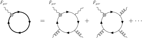
Figure 1: The effective action to linear order in $d_{Q}$ after integrating out the heavy quark. The thick line on the left hand side indicates the full heavy quark propagator with the covariant derivative $D_{\mu}$, and the cross dot indicates the EDM operator insertion. The full propagator is expanded with respect to the field strengths, which results in the $CP$-odd photon-gluon operators as shown on the right hand side.

The heavy quark EDM induces $CP$-odd photon-gluon operators through the diagrams in Fig. 1. The effective action after integrating out the heavy quark, to linear order in $d_{Q}$, is given by

$$S_{\mathrm{eff}}=-\frac{id_{Q}}{2}\mathrm{Tr}\left[\frac{1}{i\not{D}-m_{Q}}\sigma_{\mu\nu}\tilde{F}^{\mu\nu}\right],$$ (2.3)

where the trace is taken over the spinor, the color and the spacetime. We further expand this expression with respect to the field strength $H_{\mu\nu}$, given by

$$H_{\mu\nu}=g_{s}G_{\mu\nu}-eQ_{Q}F_{\mu\nu},$$ (2.4)

which satisfies $[iD_{\mu},iD_{\nu}]=iH_{\mu\nu}$. To the lowest order, we obtain (see App. B.1 for derivation)

$$\mathcal{L}_{\mathrm{eff}}=\frac{d_{Q}}{48\pi^{2}m_{Q}^{3}}\mathrm{tr}_{c}\left[-H_{\mu\nu}H^{\mu\nu}H_{\rho\sigma}\tilde{F}^{\rho\sigma}+2{H^{\mu}}_{\nu}{H^{\nu}}_{\rho}{H^{\rho}}_{\sigma}{\tilde{F}^{\sigma}}_{\mu}\right],$$ (2.5)

where $\mathrm{tr}_{c}$ is the trace only over the color. This contains $CP$-odd photon-gluon operators as well as a $CP$-odd pure photon operator. The operator quadratic in the photon field is given by

$$\mathcal{L}_{G^{2}F\tilde{F}} =\frac{eQ_{Q}g_{s}^{2}d_{Q}}{24\pi^{2}m_{Q}^{3}}\mathrm{tr}_{c}\left[F_{\mu\nu}G^{\mu\nu}\tilde{F}_{\rho\sigma}G^{\rho\sigma}-{\tilde{F}^{\mu}}_{\nu}{G^{\nu}}_{\rho}{F^{\rho}}_{\sigma}{G^{\sigma}}_{\mu}\right],$$ (2.6)

while the one linear in the photon field is given by

$$\mathcal{L}_{G^{3}\tilde{F}} =\frac{g_{s}^{3}d_{Q}}{48\pi^{2}m_{Q}^{3}}\mathrm{tr}_{c}\left[-G_{\mu\nu}G^{\mu\nu}G_{\rho\sigma}\tilde{F}^{\rho\sigma}+2{G^{\mu}}_{\nu}{G^{\nu}}_{\rho}{G^{\rho}}_{\sigma}{\tilde{F}^{\sigma}}_{\mu}\right].$$ (2.7)

Carrying out color traces explicitly, one finds that (2.6) contains $\delta^{ab}$, while (2.7) has $d^{abc}$ structure. In that sense, (2.6) would exist for any choice of the gauge group for $G_{\mu\nu}$ including a $\mathrm{U}(1)$, while (2.7) requires $N\geq 3$ for $\text{SU}(N)$, which includes of course the color group of the Standard Model.

As we will see, below the QCD scale, operator (2.6) contributes to paramagnetic EDMs through the semi-leptonic $CP$-odd operator $C_{S}$ while (2.7) contributes to the neutron EDM. The implication of the $CP$-odd pure photon operator is studied in detail in [5] in the context of the muon EDM. This operator puts only a subdominant constraint on the heavy quark EDM, and thus we do not discuss it any further in this paper.

2.2 Light quark EDMs

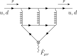
Figure 2: An example of the three-loop diagrams that generate the light quark EDMs. The cross dot indicates the heavy quark EDM $d_{Q}$ insertion, the wavy line is the external photon, the closed solid line is the heavy quark and the upper solid line is the light quark, respectively. There are five additional diagrams that are permutations of the gluon lines attached to the light quark line.

The heavy quark EDM induces the up and down quark EDMs at the three-loop level through the diagram in Fig. 2 (and its permutations), where the closed loop is the heavy quark and the cross dot indicates the heavy quark EDM insertion. In our case the heavy quark EDM operator already contains a derivative acting on the external photon, and thus we can ignore the momentum flow of the photon. The mass and the external momentum of the light quark are small compared to the heavy quark mass scale, and this allows us to expand the diagram with respect to the light quark mass and momentum. To linear order, the amplitude is schematically given by

$$i\mathcal{M}_{3\mathchar 45\relax\mathrm{loop}}=i\tilde{F}^{\mu\nu}p^{\rho}\bar{q}S_{\mu\nu\rho}q,$$ (2.8)

where $q=u,d$ is the light quark field and $p$ is the light quark momentum. Here we used the equation of motion to express quantities that explicitly depend on the light quark mass $m_{q}$ in terms of $p$. After projecting $S_{\mu\nu\rho}$ onto the EDM part, we obtain the light quark EDM $d_{q}$ as

$$d_{q}=\frac{m_{q}}{96}\mathrm{tr}\left[S_{\mu\nu\rho}\left\{\sigma^{\mu\nu},\gamma^{\rho}\right\}\right],$$ (2.9)

where the trace is taken only over the spinor index, and $\{..,..\}$ represents anticommutator. We evaluate this expression with the dimensional regularization. Since we expanded the amplitude with respect to the external momentum and the light quark mass, $S_{\mu\nu\rho}$ depends only on the heavy quark mass and hence is given by the vacuum integrals. In our case, among six propagators, three are massive and three are massless. In this case, we can reduce the vacuum integrals to two irreducible master integrals [33]. We use FIRE6 [34] to reduce the vacuum integrals by integration by parts, and use analytical expressions of the master integrals in [35]. We then obtain

$$d_{q} =\frac{5\left(8\zeta(3)-7\right)}{72}\times\left(\frac{\alpha_{s}}{\pi}\right)^{3}\frac{m_{q}}{m_{Q}}d_{Q},$$ (2.10)

where $\alpha_{s}=g_{s}^{2}/4\pi$ and $\zeta(3)\simeq 1.202$ with $\zeta(z)$ the Riemann zeta function. We have checked that all the gauge-dependent part of the gluon propagator cancels in our computation. Moreover, although each master integral is divergent, all the divergences cancel and the final result is finite. If we drop the color factors, this is equivalent to one contribution to the electron EDM from the muon/tau EDM, the diagram (a) in [3]. Our result differs from [3] and we will come back to the origin of this difference in a separate publication [36]. Notice that $d_{q}$ is suppressed only by $1/m_{Q}$ since the loop integral is dominated by the loop momentum of order $m_{Q}$, while the $CP$-odd photon-gluon operators that we computed in Sec. 2.1 are suppressed by $1/m_{Q}^{3}$. Therefore the light quark EDM is expected to be more important for heavier quarks, although there is another (and a dominant) contribution in the case of the top quark as we mentioned at the beginning of this section.

3 Paramagnetic EDM

In this section we study a constraint on the heavy quark EDM from paramagnetic atomic/molecule EDM experiments, in particular the ACME experiment [2]. The paramagnetic EDM experiments are sensitive only to a linear combination of two operators, the electron EDM $d_{e}$ and the semi-leptonic $CP$-odd operator $C_{S}$ given by

$$\mathcal{L}=C_{S}\frac{G_{F}}{\sqrt{2}}\bar{e}i\gamma_{5}e\left(\bar{p}p+\bar{n}n\right),$$ (3.1)

where $G_{F}$ is the Fermi constant, $e$ is the electron (one should not confuse it with the electromagnetic coupling), $p$ is the proton and $n$ is the neutron, respectively. It is convenient to define an equivalent electron EDM as [37]

$$d_{e}^{(\mathrm{equiv})}=d_{e}+C_{S}\times 1.5\times 10^{-20}\,e\,\mathrm{cm},$$ (3.2)

where we focus on ThO molecule. The current bound on the equivalent electron EDM is given by $|d_{e}^{(\mathrm{equiv})}|<1.1\times 10^{-29}\,e\,\mathrm{cm}$ [2].

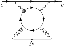
Figure 3: The diagram that generates the $CP$-odd semi-leptonic operator $C_{S}$. The photons are attached to the electron line and generate the structure $\bar{e}i\gamma_{5}e$, while the gluons feed into the nucleon $N$.

We now compute $C_{S}$ induced by the $CP$-odd photon-gluon operator, in particular the two-photon two-gluon operator, below the QCD scale. The effective Lagrangian is given by

$$\mathcal{L}_{G^{2}F\tilde{F}}=\frac{eQ_{Q}g_{s}^{2}d_{Q}}{48\pi^{2}m_{Q}^{3}}G_{\mu\nu}^{a}G^{a}_{\alpha\beta}\left(F^{\mu\nu}\tilde{F}^{\alpha\beta}-F^{\nu\alpha}\tilde{F}^{\beta\mu}\right).$$ (3.3)

Because our starting point here is explicitly isospin symmetric, it will result in the same $C_{S}$ coupling for neutrons and protons. The nucleon matrix element of the gluon part is given by

$$\langle N\rvert\frac{g_{s}^{2}}{32\pi^{2}}G^{a}_{\mu\nu}G^{a}_{\alpha\beta}\lvert N\rangle=-\frac{m_{N}}{108}\left(\eta_{\alpha\mu}\eta_{\beta\nu}-\eta_{\alpha\nu}\eta_{\beta\mu}\right)\bar{N}N+\cdots,$$ (3.4)

where $N$ is the nucleon field (either $p$ or $n$) with $m_{N}$ its mass, and $\cdots$ denotes the traceless tensor part that is irrelevant for our purpose. Here we used that, in the chiral limit, the one-loop trace anomaly dominantly contributes to the nucleon mass,

$$\langle N\rvert\frac{g_{s}^{2}}{32\pi^{2}}G_{\mu\nu}^{a}G^{a\mu\nu}\lvert N\rangle=-\frac{m_{N}}{9}\bar{N}N,$$ (3.5)

where the coefficient in the right-hand-side is related to the beta function [38]. The photons are attached to the electron and induce the operator $\bar{e}i\gamma_{5}e$ at one-loop [39] as shown in Fig. 3. This integral is logarithmically divergent, which is regulated by the heavy quark mass scale. Therefore, to the leading logarithmic accuracy, we obtain

$$C_{S}\frac{G_{F}}{\sqrt{2}}=-\frac{4Q_{Q}\alpha^{2}}{27}\frac{m_{N}m_{e}}{m_{Q}^{3}}\log\left(\frac{m_{Q}}{m_{e}}\right)\frac{d_{Q}}{e},$$ (3.6)

where $\alpha=e^{2}/4\pi$ and $m_{e}$ is the electron mass. By requiring $|{d_{e}^{(\mathrm{equiv})}}|<1.1\times 10^{-29}\,e\,\mathrm{cm}$, we obtain

$$\left|{d_{c}}\right|<1.3\times 10^{-20}\,e\,\mathrm{cm},$$ (3.7)

for the charm quark and

$$\left|{d_{b}}\right|<7.6\times 10^{-19}\,e\,\mathrm{cm},$$ (3.8)

for the bottom quark, respectively. The heavy quark EDM also induces the electron EDM at three-loop [3, 40], but its contribution to $d_{e}^{(\mathrm{equiv})}$ is negligible compared to $C_{S}$.

We now estimate the precision of our calculation. There is an uncertainty associated with Eq. (3.5), which is valid only in the chiral limit. However, the quark contribution to the nucleon mass is less than 10 % [41], and hence the uncertainty of Eq. (3.5) is also less than 10 %. Thanks to the lattice computations, these contributions are rather precisely known and the uncertainty in the non-perturbative matrix element can be further reduced by including the light quark contributions into our computation. Another uncertainty originates from our photon-loop computation, where we include only the leading logarithmic term. The uncertainty associated with this treatment may be estimated by changing the cut-off scale from $m_{Q}$ to $2m_{Q}$, which results in $\lesssim 10\,\%$ change of the result for both the charm and bottom quarks. This can be further improved by performing the full two-loop computation, with the heavy quark and photon loops at the same time. Therefore, the precision of our $C_{S}$ calculation is estimated to be 10 % and this can be further improved by properly including the quark contribution to the nucleon mass and performing the full two-loop computation of the photon-loop.

Our constraint is stronger than the one derived from $e^{+}e^{-}\to q\bar{q}$ at LEP by several orders of magnitude [25]. Although our constraint is weaker than [31] at its face value, there are two caveats. First, as we mentioned in the introduciton, the constraint in [31] is a re-interpretation of the bounds on the CEDMs $\tilde{d}_{Q}$ at the heavy quark mass scale, i.e., $\tilde{d}_{Q}(m_{Q})$. Both the quark EDM and CEDM at high energy scale $\Lambda_{\mathrm{NP}}$ contribute to the CEDM at lower energy due to the RG running, and hence $\tilde{d}_{Q}(m_{Q})$ is given as a linear combination of $d_{Q}(\Lambda_{\mathrm{NP}})$ and $\tilde{d}_{Q}(\Lambda_{\mathrm{NP}})$. With only this information, one can put a constraint on only this particular linear combination of $d_{Q}(\Lambda_{\mathrm{NP}})$ and $\tilde{d}_{Q}(\Lambda_{\mathrm{NP}})$. Therefore the authors assume that there is no huge cancellation between $d_{Q}(\Lambda_{\mathrm{NP}})$ and $\tilde{d}_{Q}(\Lambda_{\mathrm{NP}})$, which allow them to derive a constraint solely on $d_{Q}(\Lambda_{\mathrm{NP}})$ and thus on $d_{Q}(m_{Q})$. Since our constraint directly applies to $d_{Q}(m_{Q})$, it is an independent constraint, without any assumptions on the relative size of $d_{Q}(\Lambda_{\mathrm{NP}})$ and $\tilde{d}_{Q}(\Lambda_{\mathrm{NP}})$. Second, it is a complicated task to estimate the size of the neutron EDM induced by the Weinberg operator. Since [31] relies on the constraints on $\tilde{d}_{Q}(m_{Q})$ from the Weinberg operator, it has a large hadronic uncertainty. In contrast, as we have just emphasized, our computation of $C_{S}$ is precise and its uncertainty is well under control. Given the rapid progress of the paramagnetic EDM experiments, $C_{S}$ will continue providing important and clean constraints on the heavy quark EDMs. In the next section, we will see that the neutron EDM provides a stronger constraint than $C_{S}$, comparable to [31], though with a larger hadronic uncertainty.

4 Neutron EDM

In Sec. 2 we have seen that the heavy quark EDM generates the $CP$-odd photon-gluon operator and the light quark EDM. Below the QCD scale, these $CP$-odd operators in turn generate the neutron EDM $d_{n}$, whose experimental upper bound is [14]

$$\left|{d_{n}}\right|<1.8\times 10^{-26}\,e\,\mathrm{cm}.$$ (4.1)

In this section we translate this upper bound to the bound on the heavy quark EDM by estimating the size of the induced neutron EDM, with effects of the nonperturbative QCD taken into account (to the extent it is possible).

4.1 Light quark EDM contribution

We first study the neutron EDM induced by the light quark EDM $d_{n}^{(d_{q})}$. Both the QCD sum rule and the quark model suggest that [42, 1, 43]

$$d_{n}^{(d_{q})} =\frac{1}{3}\left(4d_{d}-d_{u}\right).$$ (4.2)

QCD sum rule calculations [42, 43] and more recently lattice calculations [44] give support to this simple formula within $\sim 30\%$ accuracy. We thus obtain

$$d_{n}^{(d_{q})} =\frac{5(8\zeta(3)-7)}{72}\left(\frac{\alpha_{s}}{\pi}\right)^{3}\frac{4m_{d}-m_{u}}{3m_{Q}}d_{Q}.$$ (4.3)

As we will see, there is another contribution to the neutron EDM from the $CP$-odd photon-gluon operator that leads to the QCD condensate power corrections in the light quark propagator. The rest of this section is devoted to estimate the size of this contribution.

4.2 $CP$-odd photon-gluon operator contribution

In Sec. 2.1 we saw that the heavy quark EDM generates the $CP$-odd photon-gluon operator

$$\mathcal{L}_{G^{3}\tilde{F}} =\frac{g_{s}^{3}d_{Q}}{48\pi^{2}m_{Q}^{3}}\mathrm{tr}_{c}\left[-G_{\mu\nu}G^{\mu\nu}G_{\rho\sigma}\tilde{F}^{\rho\sigma}+2{G^{\mu}}_{\nu}{G^{\nu}}_{\rho}{G^{\rho}}_{\sigma}{\tilde{F}^{\sigma}}_{\mu}\right].$$ (4.4)

Below the QCD scale the gluons confine and condense, and this operator feeds into the neutron EDM. We use the QCD sum rule technique [45] to estimate the size of the neutron EDM induced by this operator.

The starting point of the QCD sum rule is to define the two-point correlator

$$\Pi(p) \equiv i\int d^{4}xe^{ip\cdot x}\langle 0|\mathcal{T}\left\{\eta(x),\bar{\eta}(0)\right\}|0\rangle.$$ (4.5)

The interpolating function $\eta$ is typically chosen as

$$\eta(x)=j_{1}(x)+\beta j_{2}(x),$$ (4.6)

and has an overlap with the neutron one-particle state. The functions $j_{1}$ and $j_{2}$ have the same quantum numbers as the neutron and are given by

$$j_{1} =2\epsilon_{ijk}\left(d_{i}^{T}\mathcal{C}\gamma_{5}u_{j}\right)d_{k},\quad j_{2}=2\epsilon_{ijk}\left(d_{i}^{T}\mathcal{C}u_{j}\right)\gamma_{5}d_{k},$$ (4.7)

where $i,j,k$ are the color indices with $\epsilon_{ijk}$ the totally anti-symmetric tensor, and $\mathcal{C}$ is the charge conjugate matrix (see App. A for its definition). Finally $\beta$ is a redundant parameter that should disappear in an exact computation. In practice, one can choose $\beta$, e.g., to optimize the convergence of the operator production expansion (OPE). The QCD sum rule relies on the quark-hadron duality and evaluate this two point correlator $\Pi(p)$ in the hadronic (phenomenological) side and the quark (OPE) side. On the phenomenological side, $\Pi(p)$ is expressed in terms of hadronic quantities such as the neutron mass and dipole moments. On the OPE side, $\Pi(p)$ is evaluated in terms of perturbative quarks and gluons with non-perturbative effects included in the form of the QCD condensates. One then obtains an estimation of the hadronic quantities by equating these two expressions, after the Borel transformation to reduce effects of excited states. In our case, we have external electromagnetic field $F_{\mu\nu}$ multiplying three Lorentz structures that in principle we can use to derive the sum rules: $\not{p}\sigma_{\mu\nu}\not{p}$, $\{\not{p},\sigma_{\mu\nu}\}$ and $\sigma_{\mu\nu}$. In this paper, we focus on the sum rule that follows from $\not{p}\sigma_{\mu\nu}\not{p}$ since it depends most strongly on the momentum and the vacuum susceptibilities are less relevant [46]. Moreover, it is computationally simple to derive the QCD sum rule based on this structure. In the following we evaluate $\Pi(p)$ in the OPE and phenomenological sides, respectively.

OPE side.

We denote the light quark propagator as

$$\left\langle 0|\mathrm{T}\left\{q_{i}(x),\bar{q}_{j}(y)\right\}|0\right\rangle\equiv\delta_{ij}S(x,y),$$ (4.8)

where only the color-diagonal contribution is relevant for the QCD sum rule based on $\not{p}\sigma_{\mu\nu}\not{p}$ in our case. The $CP$-odd photon-gluon operator does not distinguish the up and down quarks, and thus we collectively denote $u$ and $d$ as $q$. With this expression, we obtain

$$\Pi_{\mathrm{OPE}}(p)=-24i\int d^{4}xe^{ip\cdot x} \left\{\mathrm{tr}\left[\gamma_{5}S^{c}\gamma_{5}S\right]S+S\gamma_{5}S^{c}\gamma_{5}S+\beta^{2}\left(\gamma_{5}SS^{c}S\gamma_{5}+\mathrm{tr}\left[S^{c}S\right]\gamma_{5}S\gamma_{5}\right)\right.$$

$$\left.+\beta\left(SS^{c}\gamma_{5}S\gamma_{5}+\gamma_{5}S\gamma_{5}S^{c}S+\mathrm{tr}\left[SS^{c}\gamma_{5}\right]S\gamma_{5}+\mathrm{tr}\left[S^{c}S\gamma_{5}\right]\gamma_{5}S\right)\right\},$$ (4.9)

where $S^{c}_{\alpha\beta}\equiv\left(\mathcal{C}S^{T}\mathcal{C}\right)_{\alpha\beta}$ and $S^{T}_{\alpha\beta}\equiv S_{\beta\alpha}$ with $\alpha$ and $\beta$ being the spinor indices, and the trace is taken only over the spinor index. In our case the light quark propagator has two contributions

$$S =S^{(0)}+S^{(\cancel{{CP}})},$$ (4.10)

where $S^{(0)}$ corresponds to the free quark propagator and is given by

$$S^{(0)}(x) =\frac{i\not{x}}{2\pi^{2}x^{4}},$$ (4.11)

while $S^{(\cancel{{CP}})}$ is the $CP$-odd part which we compute from now.

The source inserted into the correlator has three gluon fields, and we follow the general idea of [23] where the Weinberg operator contribution to $d_{n}$ was first evaluated, and where two gluons are treated perturbatively, while the third gluon field contributes to the quark-gluon condensate. With the QCD condensate background, we can write down the diagram

$$S_{ij}^{(\cancel{{CP}})}(p)=\leavevmode\hbox to74.38pt{\vbox to20.32pt{\text{[drawing]}}}, \scriptstyle p \scriptstyle p \scriptstyle p \scriptstyle p {\scriptstyle j} {\scriptstyle i} \scriptstyle p \scriptstyle p \scriptstyle p \scriptstyle p {\scriptstyle j} {\scriptstyle i}$$ (4.12)

where the crosses indicate the background fields, either the external photon or the QCD condensation of the quarks and gluons, and the cross dot is the insertion of the $CP$-odd photon-gluon operator (4.4). Since the QCD vacuum does not violate the Lorentz and color symmetries, we have

$$\left\langle q_{i}\bar{q}_{j}G^{a}_{\mu\nu}\right\rangle =-\frac{1}{192}T^{a}_{ij}\sigma_{\mu\nu}\left\langle\bar{q}\sigma\cdot Gq\right\rangle,$$ (4.13)

where $\sigma\cdot G=\sigma_{\mu\nu}G^{\mu\nu}$, and $\langle\cdots\rangle$ corresponds to the vacuum expectation value. We thus obtain

$$S^{(\cancel{{CP}})}_{ij}(p) =\delta_{ij}S^{(\cancel{{CP}})}(p)=i\delta_{ij}\frac{5\alpha_{s}^{2}d_{Q}}{864m_{Q}^{3}}\frac{g_{s}\langle\bar{q}\sigma\cdot Gq\rangle}{p^{2}}\frac{i}{\not{p}}\left[\sigma\cdot\tilde{F}-\frac{2p^{\mu}p^{\nu}}{p^{2}}\tilde{F}_{\mu\alpha}{\sigma_{\nu}}^{\alpha}\right]\frac{i}{\not{p}}.$$ (4.14)

Its Fourier transformation has an IR divergence, which in the dimensional regularization leads

$$S^{(\cancel{{CP}})}(x) =\frac{5\alpha_{s}^{2}d_{Q}}{27648\pi^{2}m_{Q}^{3}}g_{s}\langle\bar{q}\sigma\cdot Gq\rangle\Gamma(\epsilon_{\mathrm{IR}})\left(-\Lambda^{2}_{\mathrm{IR}}x^{2}\right)^{-\epsilon_{\mathrm{IR}}}\tilde{F}\cdot\sigma,$$ (4.15)

where we take $d_{\mathrm{IR}}=4+2\epsilon_{\mathrm{IR}}$ and keep only the logarithmic terms, with $\Lambda_{\mathrm{IR}}$ the IR cut-off scale. Due to the sensitivity to IR scale, calculations of further terms in the OPE are not possible. As a consequence, this evaluation should be viewed as an estimate, which cannot be systematically improved within QCD sum rule method. With the explicit forms of $S^{(0)}$ and $S^{(\cancel{{CP}})}$, we obtain

$$\Pi_{\mathrm{OPE}}(p)=-\frac{5\alpha_{s}^{2}d_{Q}}{2^{12}3^{3}\pi^{4}m_{Q}^{3}}\left\langle\bar{q}\sigma\cdot g_{s}Gq\right\rangle\left[\left(1-\beta\right)^{2}\not{p}\tilde{F}\cdot\sigma\not{p}-18\left(1-\beta^{2}\right)p^{2}\tilde{F}\cdot\sigma\right]I(p^{2};\epsilon_{\mathrm{IR}},\epsilon_{\mathrm{UV}}),$$ (4.16)

where we perform the dimensional regularization to tame the UV divergence with $d_{\mathrm{UV}}=4-2\epsilon_{\mathrm{UV}}$, and

$$I(p^{2};\epsilon_{\mathrm{IR}},\epsilon_{\mathrm{UV}}) \equiv\Gamma(\epsilon_{\mathrm{IR}})\left(-\frac{\Lambda_{\mathrm{IR}}^{2}}{p^{2}}\right)^{-\epsilon_{\mathrm{IR}}}\Gamma(-\epsilon_{\mathrm{UV}}-\epsilon_{\mathrm{IR}})\left(-\frac{\mu^{2}}{p^{2}}\right)^{-\epsilon_{\mathrm{UV}}},$$ (4.17)

with $\mu$ the renormalization scale. We then perform the Borel transformation, defined as [47]

$$\mathcal{B}\left[\Pi(p^{2}=-P^{2})\right] =\frac{1}{\pi}\int_{0}^{\infty}\frac{dP^{2}}{M^{2}}e^{-P^{2}/M^{2}}\mathrm{Im}\left[\Pi(p)\right]_{p^{2}=-P^{2}}.$$ (4.18)

We thus obtain the $\not{p}\sigma_{\mu\nu}\not{p}$ part as

$$\mathcal{B}\left[\Pi_{\mathrm{OPE}}(p^{2}=-P^{2})\right]_{\not{p}\tilde{F}\cdot\sigma\not{p}} =-\frac{5\alpha_{s}^{2}d_{Q}}{2^{12}3^{3}\pi^{4}m_{Q}^{3}}\left(1-\beta\right)^{2}\left\langle\bar{q}\sigma\cdot g_{s}Gq\right\rangle\log\left(\frac{M^{2}}{\Lambda_{\mathrm{IR}}^{2}}\right).$$ (4.19)

Taking the imaginary part of $I(p^{2};\epsilon_{\mathrm{IR}},\epsilon_{\mathrm{UV}})$ is somewhat subtle, and we provide details in App. B.2. There we also clarify the physical meaning of the scale $\Lambda_{\mathrm{IR}}$; it should be identified with the mass of the constituent quarks. This expression is to be compared with the phenomenological expression.

Phenomenological side.

On the phenomenological side, the two-point correlator with the neutron EDM insertion is expressed as

$$\Pi_{\mathrm{pheno}}(p)=-\lambda_{n}^{2}\left[\frac{\not{p}+m_{n}}{p^{2}-m_{n}^{2}}-\frac{d_{n}}{2(p^{2}-m_{n}^{2})^{2}}\not{p}\tilde{F}\cdot\sigma\not{p}+\cdots\right],$$ (4.20)

where $m_{n}$ is the neutron mass and $\lambda_{n}$ parametrizes the overlap between the interpolating function $\eta$ and the neutron one-particle state. After the Borel transformation, we obtain

$$\mathcal{B}\left[\Pi_{\mathrm{pheno}}(p^{2}=-P^{2})\right]_{\not{p}\tilde{F}\cdot\sigma\not{p}} =\frac{\lambda_{n}^{2}d_{n}}{2M^{4}}e^{-m_{n}^{2}/M^{2}}+\cdots,$$ (4.21)

where $\cdots$ expresses contributions from excited states which we ignore in the following.

Sum rule.

The QCD sum rule of the neutron EDM is obtained by equating Eqs. (4.19) and (4.21). We thus obtain

$$\frac{\lambda_{n}^{2}d_{n}^{(G^{3}\tilde{F})}}{2M^{4}}e^{-m_{n}^{2}/M^{2}} =-\frac{5\alpha_{s}^{2}d_{Q}}{2^{12}3^{3}\pi^{4}m_{Q}^{3}}\left(1-\beta\right)^{2}\left\langle\bar{\psi}\sigma\cdot g_{s}G\psi\right\rangle\log\left(\frac{M^{2}}{\Lambda_{\mathrm{IR}}^{2}}\right),$$ (4.22)

where $d_{n}^{(\tilde{F}G^{3})}$ is the neutron EDM induced by the $CP$-odd photon-gluon operator (to distinguish it from the one induced by the light quark EDM). We may use the Ioffe formula for the nucleon mass [48, 49]

$$\frac{\lambda_{n}^{2}m_{n}}{M^{4}}e^{-m_{n}^{2}/M^{2}}=-\frac{7-2\beta-5\beta^{2}}{16\pi^{2}}\langle\bar{q}q\rangle,$$ (4.23)

to eliminate $\lambda_{n}$. Then we obtain the QCD sum rule estimation of the neutron EDM

$$d_{n}^{(G^{3}\tilde{F})} =d_{Q}\times\frac{5\alpha_{s}^{2}}{2^{7}3^{3}\pi^{2}}\frac{m_{n}m_{0}^{2}}{m_{Q}^{3}}\frac{1-\beta}{7+5\beta}\log\left(\frac{M^{2}}{\Lambda_{\mathrm{IR}}^{2}}\right),$$ (4.24)

where we used $\langle q\sigma\cdot g_{s}Gq\rangle=m_{0}^{2}\langle\bar{q}q\rangle$ with $m_{0}^{2}=0.8\,\mathrm{GeV}^{2}$ [50].

4.3 Constraint on heavy quark EDM

The neutron EDM has two contributions, induced by the light quark EDM and the $CP$-odd photon-gluon operators, and is given by

$$d_{n}=d_{n}^{(d_{q})}+d_{n}^{(G^{3}\tilde{F})},$$ (4.25)

where

$$d_{n}^{(d_{q})} =d_{Q}\times\frac{5(8\zeta(3)-7)}{72}\left(\frac{\alpha_{s}}{\pi}\right)^{3}\frac{4m_{d}-m_{u}}{3m_{Q}},\quad d_{n}^{(G^{3}\tilde{F})}=d_{Q}\times\frac{5\alpha_{s}^{2}}{2^{7}3^{3}\pi^{2}}\frac{m_{n}m_{0}^{2}}{m_{Q}^{3}}\log\left(\frac{M^{2}}{\Lambda_{\mathrm{IR}}^{2}}\right),$$ (4.26)

and we take $\beta=-1$ following [48, 51, 52]. The parameters should be evaluated at $m_{Q}$ for the former contribution, and at the scale close to $\Lambda_{\mathrm{QCD}}$ for the latter contribution. We use $m_{c}=1.27\,\mathrm{GeV}$, $m_{b}=4.18\,\mathrm{GeV}$, $\alpha_{s}(m_{c})=0.38$ and $\alpha_{s}(m_{b})=0.223$ [53]. The light quark masses (in the $\overline{\mathrm{MS}}$ scheme) also depend on the energy scale, and we take $m_{u}(m_{c})=2.5\,\mathrm{MeV}$ $m_{d}(m_{c})=5.4\,\mathrm{MeV}$, $m_{u}(m_{b})=1.8\,\mathrm{MeV}$ and $m_{d}(m_{b})=4.0\,\mathrm{MeV}$ that we obtain by running the light quark masses at $2\,\mathrm{GeV}$ following [53]. Finally we take $\alpha_{s}=0.5$, $\Lambda_{\mathrm{IR}}=300\,\mathrm{MeV}$ and $M=800\,\mathrm{MeV}$ for the QCD sum rule estimation for definiteness. For these values, the contribution from the $CP$-odd photon-gluon operator is larger by a factor of $16$ and $10$ for the charm and bottom quarks, respectively. In the bottom quark case, the explicit quark mass suppression is compensated by the running of the strong coupling, and the $CP$-odd photon-gluon operator is still larger than the light quark EDM even with the relative suppression factor $1/m_{b}^{2}$. By requiring that $|d_{n}|<1.8\times 10^{-26}\,e\,\mathrm{cm}$, we obtain

$$\left|{d_{c}}\right| <6\times 10^{-22}\,e\,\mathrm{cm},$$ (4.27)

for the charm quark, and

$$\left|{d_{b}}\right| <2\times 10^{-20}\,e\,\mathrm{cm},$$ (4.28)

for the bottom quark, respectively.

The constraint from $d_{n}$ is stronger than that from $C_{S}$ by more than an order of magnitude. However, one should note that the estimation of $d_{n}$ has a large hadronic uncertainty. Indeed, the final result is affected by a factor two if we use the sum rule of the nucleon kinetic term instead of the mass term for $\lambda_{n}$. There are also uncertainties related to the choice of $M$ and $\beta$ which can again result in a factor of a few difference in the final result. Therefore our constraint here should be understood as an order-of-magnitude estimation and the numerical factor should be taken with care. In contrast, our calculation of $C_{S}$ is far more precise. Its uncertainty is estimated to be $\sim 10\,\%$ and can be further reduced if needed (see the end of Sec. 3). In this sense, the constraints from $d_{n}$ and $C_{S}$ are complementary to each other; $d_{n}$ puts a stronger constraint on the heavy quark EDM, while the calculation of $C_{S}$ is cleaner and its uncertainty is well under control.

Our constraint on $d_{c}$ is stronger than [31] by a factor two, while the one on $d_{b}$ is weaker by a factor two. However, as we noted in the introduction and the end of Sec. 3, our constraint directly applies to $d_{c}(m_{c})$ and $d_{b}(m_{b})$, and is independent of the one in [31].

5 Conclusion

In this paper, we have derived indirect limits on the charm and bottom quark EDMs. The charm and bottom quark EDMs generate the $CP$-odd photon-gluon operators and the light quark EDMs after integrating out the charm and bottom quarks. Photon-gluon operators contribute to the semi-leptonic $CP$-odd operator $C_{S}$ (and ultimately to paramagnetic AMO EDMs) as well as to the neutron EDM at a non-perturbative level. Quark EDM dominantly contributes to the neutron and nuclear EDMs. Performing our evaluation and using the current limits, we obtain

$$\left|{d_{c}}\right| <1.3\times 10^{-20}\,e\,\mathrm{cm},\quad\left|{d_{b}}\right|<7.6\times 10^{-19}\,e\,\mathrm{cm},$$ (5.1)

from the paramagnetic EDM experiments, and

$$\left|{d_{c}}\right| <6\times 10^{-22}\,e\,\mathrm{cm},\quad\left|{d_{b}}\right|<2\times 10^{-20}\,e\,\mathrm{cm},$$ (5.2)

from the neutron EDM experiment, respectively. Although the constraint from the neutron EDM is stronger, it has a larger hadronic uncertainty. The uncertainty of the constraint from the paramagnetic EDM is estimated as 10 % and can be improved if needed, while the uncertainty from the neutron EDM can be a factor of a few. Our constraint is independent of the one given in [31] in the sense that our constraint directly applies to the EDM operators at the quark mass threshold. By assuming a simple scaling of $d_{Q}/e\propto(\alpha/\pi)m_{Q}/\Lambda^{2}_{Q}$, we may translate our constraint as a lower bound on $CP$-odd new physics scale: $\Lambda_{c}>70\,\mathrm{GeV}$ and $\Lambda_{b}>20\,\mathrm{GeV}$ from the paramagnetic EDM experiment, and $\Lambda_{c}>300\,\mathrm{GeV}$ and $\Lambda_{b}>100\,\mathrm{GeV}$ from the neutron EDM experiment.

Our result provides an important benchmark to overcome for the LHC based measurements of the charmed baryon EDMs [26, 27, 28, 29, 30]. The idea of using the bent crystal technique for studying electromagnetic properties of baryons containing a heavy quark is very appealing. However, given the strength of the bounds derived in our work, and the necessity to satisfy independent constraints from $d_{n}$ and $C_{S}$ (hence removing a chance of accidentally large $d_{c(b)}$ due to cancellations), one may want to re-evaluate the main goal of the charmed baryon experiment. While it will be difficult to match the indirect sensitivity to $d_{c(b)}$, the planned measurement may achieve sufficient accuracy to extract the values of the magnetic moments $\mu_{c(b)}$ and compare it with the QCD predictions.

Acknowledgements

Y.E. and M.P. are supported in part by U.S. Department of Energy Grant No. de-sc0011842. M.P. would like to thank Dr. K. Melnikov for the advice in evaluating loop contributions. The Feynman diagrams in this paper are generated by TikZ-Feynman [54].

Appendix A Convention

Here we summarize our conventions used in this paper. The field strengths are given by

$$F_{\mu\nu} =\partial_{\mu}A_{\nu}-\partial_{\nu}A_{\mu},\quad G_{\mu\nu}^{a}=\partial_{\mu}G_{\nu}^{a}-\partial_{\nu}G^{a}_{\mu}+g_{s}f^{abc}G_{\mu}^{b}G_{\nu}^{c},\quad G_{\mu\nu}=G_{\mu\nu}^{a}T^{a},$$ (A.1)

where $f^{abc}$ is the SU(3) structure constant. The SU(3) generator satisfies

$$\left[T^{a},T^{b}\right]=if^{abc}T^{c},\quad\mathrm{tr}_{\mathrm{c}}\left[T^{a}T^{b}\right]=\frac{\delta^{ab}}{2}.$$ (A.2)

The dual field strengths are defined as

$$\tilde{F}^{\mu\nu}=\frac{1}{2}\epsilon^{\mu\nu\rho\sigma}F_{\rho\sigma},\quad\tilde{G}^{\mu\nu}=\frac{1}{2}\epsilon^{\mu\nu\rho\sigma}G_{\rho\sigma},$$ (A.3)

with $\epsilon^{0123}=+1$. We take the gamma matrix as

$$\left\{\gamma^{\mu},\gamma^{\nu}\right\}=2\eta^{\mu\nu},\quad\eta_{\mu\nu}=\mathrm{diag}(+,-,-,-),\quad\gamma_{5}=i\gamma^{0}\gamma^{1}\gamma^{2}\gamma^{3}=-\frac{i}{4!}\epsilon^{\mu\nu\rho\sigma}\gamma_{\mu}\gamma_{\nu}\gamma_{\rho}\gamma_{\sigma},$$ (A.4)

and $\sigma_{\mu\nu}$ as

$$\sigma_{\mu\nu}=\frac{i}{2}\left(\gamma_{\mu}\gamma_{\nu}-\gamma_{\nu}\gamma_{\mu}\right)=\frac{i}{2}\left[\gamma_{\mu},\gamma_{\nu}\right].$$ (A.5)

The charge conjugation matrix $\mathcal{C}$ satisfies

$$\left(\gamma^{\mu}\right)^{T}\mathcal{C}=-\mathcal{C}\gamma^{\mu},$$ (A.6)

such that $\psi^{T}\mathcal{C}$ has the same Lorentz transformation property as $\bar{\psi}$. In the Weyl representation it is given by

$$\mathcal{C}=i\gamma^{0}\gamma^{2}.$$ (A.7)

Appendix B Technical details

In this appendix we provide some technical details that we omit in the main text.

B.1 Derivation of $CP$-odd photon-gluon operators

In this subsection we provide derivation of the $CP$-odd photon-gluon operators (2.5) after integrating out the heavy quarks (see [55] for an extensive review on this procedure). Our starting point is Eq. (2.3). We can simplify it as

$$S_{\mathrm{eff}} =-\frac{id_{Q}}{2}\mathrm{Tr}\left[\frac{i\not{D}+m_{Q}}{i\not{D}+m_{Q}}\frac{1}{i\not{D}-m_{Q}}\sigma_{\mu\nu}\tilde{F}^{\mu\nu}\right]=-\frac{id_{Q}m_{Q}}{2}\mathrm{Tr}\left[\frac{1}{\left(iD\right)^{2}-m_{Q}^{2}+\frac{1}{2}\sigma\cdot H}(\sigma\cdot\tilde{F})\right],$$ (B.1)

where $(iD)^{2}=iD_{\mu}iD^{\mu}$ and we used that the traces of odd $\gamma$’s vanish in the second equality. We further expand the denominator with respect to $H$, and obtain up to fourth-order in the gauge fields

$$S_{\mathrm{eff}} =-\frac{id_{Q}m_{Q}}{2}\left(T_{2}+T_{3}+T_{4}\right),$$ (B.2)

where

$$T_{2} =-\frac{1}{2}\mathrm{Tr}\left[\frac{1}{\left(iD\right)^{2}-m_{Q}^{2}}(\sigma\cdot H)\frac{1}{\left(iD\right)^{2}-m_{Q}^{2}}(\sigma\cdot\tilde{F})\right],$$ (B.3)

$$T_{3} =+\frac{1}{4}\mathrm{Tr}\left[\frac{1}{\left(iD\right)^{2}-m_{q}^{2}}(\sigma\cdot H)\frac{1}{\left(iD\right)^{2}-m_{Q}^{2}}(\sigma\cdot H)\frac{1}{\left(iD\right)^{2}-m_{Q}^{2}}(\sigma\cdot\tilde{F})\right],$$ (B.4)

$$T_{4} =-\frac{1}{8}\mathrm{Tr}\left[\frac{1}{\left(iD\right)^{2}-m_{Q}^{2}}(\sigma\cdot H)\frac{1}{\left(iD\right)^{2}-m_{Q}^{2}}(\sigma\cdot H)\frac{1}{\left(iD\right)^{2}-m_{Q}^{2}}(\sigma\cdot H)\frac{1}{\left(iD\right)^{2}-m_{Q}^{2}}(\sigma\cdot\tilde{F})\right].$$ (B.5)

The term linear in $\sigma_{\mu\nu}$ vanishes after taking the trace of the spinor index. In order to compute $T_{2}$, we use the following identity [55]:

$$\mathrm{Tr}\left[\frac{1}{\left((iD)^{2}-m_{q}^{2}\right)^{3}}f(H,F)\right] =\mathrm{Tr}\left[\frac{1}{\left((i\partial)^{2}-m_{q}^{2}\right)^{3}}f(H,F)\right]-\mathrm{Tr}\left[\frac{1}{\left((iD)^{2}-m_{q}^{2}\right)^{5}}H_{\mu\nu}H^{\mu\nu}f(H,F)\right],$$ (B.6)

where $f(H,F)$ is an arbitrary function of $H_{\mu\nu}$ and $F_{\mu\nu}$. We thus obtain

$$\frac{d}{dm_{Q}^{2}}T_{2} =-\mathrm{Tr}\left[\frac{1}{((i\partial)^{2}-m_{Q}^{2})^{3}}\left(\sigma\cdot H\right)\sigma\cdot\tilde{F}\right]+\mathrm{Tr}\left[\frac{1}{((iD)^{2}-m_{Q}^{2})^{5}}H_{\mu\nu}H^{\mu\nu}\left(\sigma\cdot H\right)\sigma\cdot\tilde{F}\right].$$ (B.7)

where we ignore the derivatives acting on $F$. We can now replace $iD$ by $i\partial$ in the last term to the order of our interest, and obtain

$$\frac{d}{dm_{Q}^{2}}T_{2} =-i\int d^{4}x\left[\frac{3eQ_{Q}}{4\pi^{2}m_{Q}^{2}}F_{\mu\nu}\tilde{F}^{\mu\nu}+\frac{1}{24\pi^{2}m_{Q}^{6}}\mathrm{tr}_{c}\left[H_{\mu\nu}H^{\mu\nu}H_{\rho\sigma}\tilde{F}^{\rho\sigma}\right]\right].$$ (B.8)

By integrating this we obtain

$$T_{2} =i\int d^{4}x\left[\frac{3eQ_{Q}}{4\pi^{2}}\ln\left(\frac{M_{R}^{2}}{m_{Q}^{2}}\right)F_{\mu\nu}\tilde{F}^{\mu\nu}+\frac{1}{48\pi^{2}m_{Q}^{4}}\mathrm{tr}_{c}\left[H_{\mu\nu}H^{\mu\nu}H_{\rho\sigma}\tilde{F}^{\rho\sigma}\right]\right],$$ (B.9)

where the additional mass scale $M_{R}$ comes from the regularization which we did not write down explicitly. Next we compute $T_{3}$. By ignoring the derivatives acting on $\tilde{F}_{\mu\nu}$, we obtain

$$T_{3}=\frac{1}{4}\mathrm{Tr} \left[\frac{1}{((iD)^{2}-m_{Q}^{2})^{3}}\left(\sigma\cdot H\right)^{2}(\sigma\cdot\tilde{F})+\frac{1}{((iD)^{2}-m_{Q}^{2})^{4}}\left[(iD)^{2},\sigma\cdot H\right](\sigma\cdot H)(\sigma\cdot\tilde{F})\right.$$

$$\left.-\frac{1}{((iD)^{2}-m_{Q}^{2})^{5}}\left[(iD)^{2},\sigma\cdot H\right]\left[(iD)^{2},\sigma\cdot H\right]\sigma\cdot\tilde{F}+\cdots\right],$$ (B.10)

where the dots indicate terms that contain more than two commutators and thus correspond to higher dimensional operators that are out of our interest. The first term is easily seen to generate only $\mathcal{O}(H^{4}\tilde{F})$ operators with the help of the identity (B.6). The second term is expanded as

$$\mathrm{Tr}\left[\frac{1}{((iD)^{2}-m_{Q}^{2})^{4}}\left[(iD)^{2},\sigma\cdot H\right](\sigma\cdot H)(\sigma\cdot\tilde{F})\right]=\mathrm{Tr} \left[\frac{1}{((iD)^{2}-m_{Q}^{2})^{4}}iD^{\alpha}\left[iD_{\alpha},\sigma\cdot H\right](\sigma\cdot H)\sigma\cdot\tilde{F}\right.$$

$$\left.+iD^{\alpha}\frac{1}{((iD)^{2}-m_{Q}^{2})^{4}}\left[iD_{\alpha},\sigma\cdot H\right](\sigma\cdot H)\sigma\cdot\tilde{F}\right.$$

$$\left.+\frac{1}{((iD)^{2}-m_{Q}^{2})^{4}}\left[iD^{\alpha},\sigma\cdot H\right]\left[iD_{\alpha},\sigma\cdot H\right]\sigma\cdot\tilde{F}\right].$$ (B.11)

The first two terms induce only higher order terms [55], and thus we ignore them. The third term in Eq. (B.10) already contains three field strengths and two commutators, and hence we can ignore any further commutators between $D$ and $H$. By taking the angular average, we obtain

$$\mathrm{Tr}\left[\frac{1}{((iD)^{2}-m_{Q}^{2})^{5}}\left[(iD)^{2},\sigma\cdot H\right]\left[(iD)^{2},\sigma\cdot H\right]\sigma\cdot\tilde{F}\right] =\mathrm{Tr}\left[\frac{(iD)^{2}}{((iD)^{2}-m_{Q}^{2})^{5}}\left[iD^{\alpha},\sigma\cdot H\right]\left[iD_{\alpha},\sigma\cdot H\right]\sigma\cdot\tilde{F}\right].$$ (B.12)

By combining them, we obtain

$$T_{3} =-\frac{m_{Q}^{2}}{4}\mathrm{Tr}\left[\frac{1}{((iD)^{2}-m_{Q}^{2})^{5}}\left[iD^{\alpha},\sigma\cdot H\right]\left[iD_{\alpha},\sigma\cdot H\right]\sigma\cdot\tilde{F}\right]$$

$$=-\frac{g_{s}^{2}}{24\pi^{2}m_{Q}^{4}}\int d^{4}x\,\mathrm{tr}_{c}\left[(\mathcal{D}^{\alpha}G_{\mu\rho})(\mathcal{D}_{\alpha}{G_{\nu}}^{\rho})\right]\tilde{F}^{\mu\nu}=0.$$ (B.13)

Finally we compute $T_{4}$. To the order of our interest, we can simply replace $iD$ by $i\partial$ in the denominator. It is then easy to see that

$$T_{4}=-\frac{i}{48\pi^{2}m_{Q}^{4}}\int d^{4}x\,\mathrm{tr}_{c}\left[3H_{\mu\nu}H^{\mu\nu}H_{\rho\sigma}\tilde{F}^{\rho\sigma}-4{H^{\mu}}_{\nu}{H^{\nu}}_{\rho}{H^{\rho}}_{\sigma}{\tilde{F}^{\sigma}}_{\mu}\right].$$ (B.14)

Therefore we obtain

$$S_{\mathrm{eff}}=\frac{d_{Q}}{48\pi^{2}m_{Q}^{3}}\int d^{4}x\,\mathrm{tr}_{c}\left[-H_{\mu\nu}H^{\mu\nu}H_{\rho\sigma}\tilde{F}^{\rho\sigma}+2{H^{\mu}}_{\nu}{H^{\nu}}_{\rho}{H^{\rho}}_{\sigma}{\tilde{F}^{\sigma}}_{\mu}\right],$$ (B.15)

where we ignored the quadratic term that is irrelevant for our purpose. If we drop the gluons, it correctly reduces to the result in [5].

B.2 Borel transformation and IR divergence

In this subsection we discuss the Borel transformation of Eq. (4.16) that contains both the UV and IR divergences. As the Borel transformation is related to the imaginary part, it is equivalent to taking the imaginary part of

$$I(p^{2};\epsilon_{\mathrm{IR}},\epsilon_{\mathrm{UV}}) \equiv\Gamma(\epsilon_{\mathrm{IR}})\left(-\frac{\Lambda_{\mathrm{IR}}^{2}}{p^{2}}\right)^{-\epsilon_{\mathrm{IR}}}\Gamma(-\epsilon_{\mathrm{UV}}-\epsilon_{\mathrm{IR}})\left(-\frac{\Lambda_{\mathrm{UV}}^{2}}{p^{2}}\right)^{-\epsilon_{\mathrm{UV}}}.$$ (B.16)

The limit of this function at $\epsilon_{\mathrm{UV}}\to 0,\>\epsilon_{\mathrm{IR}}\to 0$ is not well defined. For example, if the limit is taken along the line $\epsilon_{\mathrm{UV}}=a\,\epsilon_{\mathrm{IR}}$ with fixed $a$, one would get an $a$-dependent result:

$$\underset{\epsilon_{\mathrm{IR}}\rightarrow 0}{\text{lim}}I(p^{2};\epsilon_{\mathrm{IR}},a\,\epsilon_{\mathrm{IR}})=-\frac{1}{2\left(1+a\right)}\left[\text{log}^{2}\left(-\frac{\Lambda_{\mathrm{IR}}^{2}}{p^{2}}\right)+2a\text{log}\left(-\frac{\Lambda_{\mathrm{IR}}^{2}}{p^{2}}\right)\text{log}\left(-\frac{\Lambda_{\mathrm{UV}}^{2}}{p^{2}}\right)+a^{2}\text{log}^{2}\left(-\frac{\Lambda_{\mathrm{UV}}^{2}}{p^{2}}\right)\right],$$ (B.17)

where we only kept the double logarithmic terms. The purpose of this subsection is to understand the correct prescription of evaluating the imaginary part of this function.

In order to understand the correct prescription, it is helpful to consider a simpler example: a scalar three-body decay. Indeed, the two point correlator $\Pi(p)$ contains three quark propagators, and thus the imaginary part of this function is related a three-body decay phase space integral. Therefore we consider the following Lagrangian

$$\mathcal{L}=\frac{1}{2}\left(\partial\phi\right)^{2}-\frac{m_{\phi}^{2}}{2}\phi^{2}+\frac{1}{2}\left(\partial\chi\right)^{2}-\frac{m_{\chi}^{2}}{2}\chi^{2}-\frac{\lambda}{6}\phi\chi^{3},$$ (B.18)

and study the three-body decay $\phi\to 3\chi$. The two-loop diagram is evaluated as

$$i\mathcal{M}_{2} =\leavevmode\hbox to0pt{\vbox to0pt{\text{[drawing]}}}=\frac{i\lambda^{2}}{6}\int\frac{d^{4}l_{1}}{(2\pi)^{4}}\int\frac{d^{4}l_{2}}{(2\pi)^{4}}D_{F}(l_{1})D_{F}(l_{2})D_{F}(l_{1}+l_{2}-p), \scriptstyle p \scriptstyle p \scriptstyle p \scriptstyle p \scriptstyle p \scriptstyle p \scriptstyle p \scriptstyle p \scriptstyle p \scriptstyle p \scriptstyle p \scriptstyle p$$ (B.19)

where $D_{F}(p)$ is the Feynman propagator,

$$iD_{F}(p)=\frac{i}{p^{2}-m_{\chi}^{2}+i0},$$ (B.20)

and the solid line is $\chi$ while the dashed line is $\phi$. The cutting rule tells us that

$$\mathrm{Im}\mathcal{M}_{2} =\frac{1}{2}\frac{\lambda^{2}}{6}\int d\Pi_{\mathrm{LIPS}},$$ (B.21)

where $d\Pi_{\mathrm{LIPS}}$ is the three-body Lorentz invariant phase space integral. This is expanded with respect to $m_{\chi}^{2}/m_{\phi}^{2}$ as

$$\int d\Pi_{\mathrm{LIPS}} =\frac{1}{32\pi^{3}}\left[\frac{m_{\phi}^{2}}{8}+\frac{3m_{\chi}^{2}}{4}\left(\log\left(\frac{4m_{\chi}^{2}}{m_{\phi}^{2}}\right)-1\right)+\cdots\right],$$ (B.22)

where we used $p^{2}=m_{\phi}^{2}$. We now evaluate the left hand side of Eq. (B.21) in an analogous way as the main text. We may expand the propagator as

$$iD_{F}(p)=\frac{i}{p^{2}-m_{\chi}^{2}}=i\left(\frac{1}{p^{2}}+\frac{1}{p^{2}}m_{\chi}^{2}\frac{1}{p^{2}}+\cdots\right),$$ (B.23)

where we omit $i\epsilon$ for notational simplicity. In the coordinate space this is given by

$$iD_{F}(x) =-\frac{1}{4\pi^{2}x^{2}}-\frac{m_{\chi}^{2}}{16\pi^{2}}\Gamma(\epsilon_{\mathrm{IR}})\left(-\Lambda_{\mathrm{IR}}^{2}x^{2}\right)^{-\epsilon_{\mathrm{IR}}}+\cdots.$$ (B.24)

The first order term in $m_{\chi}^{2}$ is IR divergent and this is analogous to our propagator with the $CP$-odd operator insertion in Sec. 4.2. The two-loop amplitude is given by

$$i\mathcal{M}_{2}(p) =\frac{\left(i\lambda\right)^{2}}{6}\mu_{\mathrm{UV}}^{d_{\mathrm{UV}}-4}\int d^{d_{\mathrm{UV}}}x\,e^{ip\cdot x}iD_{F}(x)iD_{F}(x)iD_{F}(x).$$ (B.25)

To the first order in $m_{\chi}^{2}$ we obtain

$$\left.\mathcal{M}_{2}\right|_{\mathcal{O}(m_{\chi}^{2})} =-\frac{\lambda^{2}m_{\chi}^{2}}{512\pi^{4}}I(p^{2};\epsilon_{\mathrm{IR}},\epsilon_{\mathrm{UV}}).$$ (B.26)

Note that we get exactly the same function $I(p^{2};\epsilon_{\mathrm{IR}},\epsilon_{\mathrm{UV}})$ here. Eq. (B.21) tells us that

$$\left.\mathrm{Im}\mathcal{M}_{2}\right|_{\mathcal{O}(m_{\chi}^{2})} =\left[\frac{1}{2}\frac{\lambda^{2}}{6}\int d\Pi_{\mathrm{LIPS}}\right]_{\mathcal{O}(m_{\chi}^{2})}=\frac{\lambda^{2}m_{\chi}^{2}}{512\pi^{3}}\log\left(\frac{m_{\chi}^{2}}{m_{\phi}^{2}}\right),$$ (B.27)

where we focus on the leading logarithmic term on the right hand side. Thus the correct prescription of evaluating the imaginary part of $I$ is

$$\mathrm{Im}\left[I(p^{2};\epsilon_{\mathrm{IR}},\epsilon_{\mathrm{UV}})\right] =-\pi\log\left(\frac{\Lambda_{\mathrm{IR}}^{2}}{p^{2}}\right),$$ (B.28)

where we identify $\Lambda_{\mathrm{IR}}^{2}=m_{\chi}^{2}$ in the present case. This agrees with the Borel transformation formula in [52]. For the example in Eq.(B.17), this prescription is equivalent to neglecting the real part of the UV logarithm.

Our discussion clarifies the physical meaning of $\Lambda_{\mathrm{IR}}$ that appears in Eq. (4.19). This IR divergence originates from the phase space integral and is regulated by the mass of the daughter particles. In the neutron EDM case, the daughter particles are the constituent quarks. Therefore $\Lambda_{\mathrm{IR}}$ is identified with the mass of the constituent up and down quarks that we take $\Lambda_{\mathrm{IR}}=300\,\mathrm{MeV}$ in the main text.

References

- [1] M. Pospelov and A. Ritz, “Electric dipole moments as probes of new physics,” Annals Phys. 318 (2005) 119–169, arXiv:hep-ph/0504231.
- [2] ACME Collaboration, V. Andreev et al., “Improved limit on the electric dipole moment of the electron,” Nature 562 no. 7727, (2018) 355–360.
- [3] A. G. Grozin, I. B. Khriplovich, and A. S. Rudenko, “Electric dipole moments, from e to tau,” Phys. Atom. Nucl. 72 (2009) 1203–1205, arXiv:0811.1641 [hep-ph].
- [4] B. Graner, Y. Chen, E. G. Lindahl, and B. R. Heckel, “Reduced Limit on the Permanent Electric Dipole Moment of Hg199,” Phys. Rev. Lett. 116 no. 16, (2016) 161601, arXiv:1601.04339 [physics.atom-ph]. [Erratum: Phys. Rev. Lett.119,no.11,119901(2017)].
- [5] Y. Ema, T. Gao, and M. Pospelov, “Improved Indirect Limits on Muon Electric Dipole Moment,” Phys. Rev. Lett. 128 no. 13, (2022) 131803, arXiv:2108.05398 [hep-ph].
- [6] T. Aoyama et al., “The anomalous magnetic moment of the muon in the Standard Model,” Phys. Rept. 887 (2020) 1–166, arXiv:2006.04822 [hep-ph].
- [7] Muon g-2 Collaboration, B. Abi et al., “Measurement of the Positive Muon Anomalous Magnetic Moment to 0.46 ppm,” Phys. Rev. Lett. 126 no. 14, (2021) 141801, arXiv:2104.03281 [hep-ex].
- [8] Muon (g-2) Collaboration, G. W. Bennett et al., “An Improved Limit on the Muon Electric Dipole Moment,” Phys. Rev. D 80 (2009) 052008, arXiv:0811.1207 [hep-ex].
- [9] Y. K. Semertzidis et al., “Sensitive search for a permanent muon electric dipole moment,” in KEK International Workshop on High Intensity Muon Sources (HIMUS 99), pp. 81–96. 12, 1999. arXiv:hep-ph/0012087.
- [10] H. Iinuma, H. Nakayama, K. Oide, K.-i. Sasaki, N. Saito, T. Mibe, and M. Abe, “Three-dimensional spiral injection scheme for the g-2/EDM experiment at J-PARC,” Nucl. Instrum. Meth. A 832 (2016) 51–62.
- [11] M. Abe et al., “A New Approach for Measuring the Muon Anomalous Magnetic Moment and Electric Dipole Moment,” PTEP 2019 no. 5, (2019) 053C02, arXiv:1901.03047 [physics.ins-det].
- [12] A. Adelmann et al., “Search for a muon EDM using the frozen-spin technique,” arXiv:2102.08838 [hep-ex].
- [13] E. M. Purcell and N. F. Ramsey, “On the Possibility of Electric Dipole Moments for Elementary Particles and Nuclei,” Phys. Rev. 78 (1950) 807–807.
- [14] C. Abel et al., “Measurement of the Permanent Electric Dipole Moment of the Neutron,” Phys. Rev. Lett. 124 no. 8, (2020) 081803, arXiv:2001.11966 [hep-ex].
- [15] V. M. Khatsimovsky, I. B. Khriplovich, and A. R. Zhitnitsky, “Strange Quarks in the Nucleon and Neutron Electric Dipole Moment,” Z. Phys. C 36 (1987) 455.
- [16] K. Fuyuto, J. Hisano, N. Nagata, and K. Tsumura, “QCD Corrections to Quark (Chromo)Electric Dipole Moments in High-scale Supersymmetry,” JHEP 12 (2013) 010, arXiv:1308.6493 [hep-ph].
- [17] V. Cirigliano, W. Dekens, J. de Vries, and E. Mereghetti, “Is there room for CP violation in the top-Higgs sector?,” Phys. Rev. D 94 no. 1, (2016) 016002, arXiv:1603.03049 [hep-ph].
- [18] V. Cirigliano, W. Dekens, J. de Vries, and E. Mereghetti, “Constraining the top-Higgs sector of the Standard Model Effective Field Theory,” Phys. Rev. D 94 no. 3, (2016) 034031, arXiv:1605.04311 [hep-ph].
- [19] S. Weinberg, “Larger Higgs Exchange Terms in the Neutron Electric Dipole Moment,” Phys. Rev. Lett. 63 (1989) 2333.
- [20] D. Chang, W.-Y. Keung, C. S. Li, and T. C. Yuan, “QCD Corrections to CP Violation From Color Electric Dipole Moment of Quark,” Phys. Lett. B 241 (1990) 589–592.
- [21] G. Boyd, A. K. Gupta, S. P. Trivedi, and M. B. Wise, “Effective Hamiltonian for the Electric Dipole Moment of the Neutron,” Phys. Lett. B 241 (1990) 584–588.
- [22] M. Dine and W. Fischler, “Constraints on New Physics From Weinberg’s Analysis of the Neutron Electric Dipole Moment,” Phys. Lett. B 242 (1990) 239–244.
- [23] D. A. Demir, M. Pospelov, and A. Ritz, “Hadronic EDMs, the Weinberg operator, and light gluinos,” Phys. Rev. D 67 (2003) 015007, arXiv:hep-ph/0208257.
- [24] F. Sala, “A bound on the charm chromo-EDM and its implications,” JHEP 03 (2014) 061, arXiv:1312.2589 [hep-ph].
- [25] A. E. Blinov and A. S. Rudenko, “Upper Limits on Electric and Weak Dipole Moments of tau-Lepton and Heavy Quarks from e+ e- Annihilation,” Nucl. Phys. B Proc. Suppl. 189 (2009) 257–259, arXiv:0811.2380 [hep-ph].
- [26] V. G. Baryshevsky, “The possibility to measure the magnetic moments of short-lived particles (charm and beauty baryons) at LHC and FCC energies using the phenomenon of spin rotation in crystals,” Phys. Lett. B 757 (2016) 426–429.
- [27] F. J. Botella, L. M. Garcia Martin, D. Marangotto, F. M. Vidal, A. Merli, N. Neri, A. Oyanguren, and J. R. Vidal, “On the search for the electric dipole moment of strange and charm baryons at LHC,” Eur. Phys. J. C 77 no. 3, (2017) 181, arXiv:1612.06769 [hep-ex].
- [28] A. S. Fomin et al., “Feasibility of measuring the magnetic dipole moments of the charm baryons at the LHC using bent crystals,” JHEP 08 (2017) 120, arXiv:1705.03382 [hep-ph].
- [29] E. Bagli et al., “Electromagnetic dipole moments of charged baryons with bent crystals at the LHC,” Eur. Phys. J. C 77 no. 12, (2017) 828, arXiv:1708.08483 [hep-ex]. [Erratum: Eur.Phys.J.C 80, 680 (2020)].
- [30] S. Aiola et al., “Progress towards the first measurement of charm baryon dipole moments,” Phys. Rev. D 103 no. 7, (2021) 072003, arXiv:2010.11902 [hep-ex].
- [31] H. Gisbert and J. Ruiz Vidal, “Improved bounds on heavy quark electric dipole moments,” Phys. Rev. D 101 no. 11, (2020) 115010, arXiv:1905.02513 [hep-ph].
- [32] U. Haisch and G. Koole, “Beautiful and charming chromodipole moments,” JHEP 09 (2021) 133, arXiv:2106.01289 [hep-ph].
- [33] D. J. Broadhurst, “Three loop on-shell charge renormalization without integration: Lambda-MS (QED) to four loops,” Z. Phys. C 54 (1992) 599–606.
- [34] A. V. Smirnov and F. S. Chuharev, “FIRE6: Feynman Integral REduction with Modular Arithmetic,” Comput. Phys. Commun. 247 (2020) 106877, arXiv:1901.07808 [hep-ph].
- [35] S. P. Martin and D. G. Robertson, “Evaluation of the general 3-loop vacuum Feynman integral,” Phys. Rev. D 95 no. 1, (2017) 016008, arXiv:1610.07720 [hep-ph].
- [36] Y. Ema, T. Gao and M. Pospelov, in preparation.
- [37] M. Pospelov and A. Ritz, “CKM benchmarks for electron electric dipole moment experiments,” Phys. Rev. D 89 no. 5, (2014) 056006, arXiv:1311.5537 [hep-ph].
- [38] M. A. Shifman, A. I. Vainshtein, and V. I. Zakharov, “Remarks on Higgs Boson Interactions with Nucleons,” Phys. Lett. B 78 (1978) 443–446.
- [39] V. V. Flambaum, M. Pospelov, A. Ritz, and Y. V. Stadnik, “Sensitivity of EDM experiments in paramagnetic atoms and molecules to hadronic CP violation,” Phys. Rev. D 102 no. 3, (2020) 035001, arXiv:1912.13129 [hep-ph].
- [40] A. G. Grozin, I. B. Khriplovich, and A. S. Rudenko, “Upper limits on electric dipole moments of tau-lepton, heavy quarks, and W-boson,” Nucl. Phys. B 821 (2009) 285–290, arXiv:0902.3059 [hep-ph].
- [41] J. Ellis, N. Nagata, and K. A. Olive, “Uncertainties in WIMP Dark Matter Scattering Revisited,” Eur. Phys. J. C 78 no. 7, (2018) 569, arXiv:1805.09795 [hep-ph].
- [42] M. Pospelov and A. Ritz, “Neutron EDM from electric and chromoelectric dipole moments of quarks,” Phys. Rev. D 63 (2001) 073015, arXiv:hep-ph/0010037.
- [43] J. Hisano, J. Y. Lee, N. Nagata, and Y. Shimizu, “Reevaluation of Neutron Electric Dipole Moment with QCD Sum Rules,” Phys. Rev. D 85 (2012) 114044, arXiv:1204.2653 [hep-ph].
- [44] T. Bhattacharya, V. Cirigliano, S. Cohen, R. Gupta, H.-W. Lin, and B. Yoon, “Axial, Scalar and Tensor Charges of the Nucleon from 2+1+1-flavor Lattice QCD,” Phys. Rev. D 94 no. 5, (2016) 054508, arXiv:1606.07049 [hep-lat].
- [45] M. A. Shifman, A. I. Vainshtein, and V. I. Zakharov, “QCD and Resonance Physics. Theoretical Foundations,” Nucl. Phys. B 147 (1979) 385–447.
- [46] H.-x. He and X.-D. Ji, “QCD sum rule calculation for the tensor charge of the nucleon,” Phys. Rev. D 54 (1996) 6897–6902, arXiv:hep-ph/9607408.
- [47] B. L. Ioffe and A. V. Smilga, “Nucleon Magnetic Moments and Magnetic Properties of Vacuum in QCD,” Nucl. Phys. B 232 (1984) 109–142.
- [48] B. L. Ioffe, “Calculation of Baryon Masses in Quantum Chromodynamics,” Nucl. Phys. B 188 (1981) 317–341. [Erratum: Nucl.Phys.B 191, 591–592 (1981)].
- [49] D. B. Leinweber, “QCD sum rules for skeptics,” Annals Phys. 254 (1997) 328–396, arXiv:nucl-th/9510051.
- [50] V. M. Belyaev and B. L. Ioffe, “Determination of Baryon and Baryonic Resonance Masses from QCD Sum Rules. 1. Nonstrange Baryons,” Sov. Phys. JETP 56 (1982) 493–501.
- [51] B. L. Ioffe, “ON THE CHOICE OF QUARK CURRENTS IN THE QCD SUM RULES FOR BARYON MASSES,” Z. Phys. C 18 (1983) 67.
- [52] U. Haisch and A. Hala, “Sum rules for CP-violating operators of Weinberg type,” JHEP 11 (2019) 154, arXiv:1909.08955 [hep-ph].
- [53] Particle Data Group Collaboration, P. A. Zyla et al., “Review of Particle Physics,” PTEP 2020 no. 8, (2020) 083C01.
- [54] J. Ellis, “TikZ-Feynman: Feynman diagrams with TikZ,” Comput. Phys. Commun. 210 (2017) 103–123, arXiv:1601.05437 [hep-ph].
- [55] V. A. Novikov, M. A. Shifman, A. I. Vainshtein, and V. I. Zakharov, “Calculations in External Fields in Quantum Chromodynamics. Technical Review,” Fortsch. Phys. 32 (1984) 585.