Supporting Vision-Language Model Inference with Causality-pruning Knowledge Prompt

Abstract.

Vision-language models are pre-trained by aligning image-text pairs in a common space so that the models can deal with open-set visual concepts by learning semantic information from textual labels. To boost the transferability of these models on downstream tasks in a zero-shot manner, recent works explore generating fixed or learnable prompts, i.e., classification weights are synthesized from natural language describing task-relevant categories, to reduce the gap between tasks in the training and test phases. However, how and what prompts can improve inference performance remains unclear. In this paper, we explicitly provide exploration and clarify the importance of including semantic information in prompts, while existing prompt methods generate prompts without exploring the semantic information of textual labels. A challenging issue is that manually constructing prompts, with rich semantic information, requires domain expertise and is extremely time-consuming. To this end, we propose Causality-pruning Knowledge Prompt (CapKP) for adapting pre-trained vision-language models to downstream image recognition. CapKP retrieves an ontological knowledge graph by treating the textual label as a query to explore task-relevant semantic information. To further refine the derived semantic information, CapKP introduces causality-pruning by following the first principle of Granger causality. Empirically, we conduct extensive evaluations to demonstrate the effectiveness of CapKP, e.g., with 8 shots, CapKP outperforms the manual-prompt method by 12.51% and the learnable-prompt method by 1.39% on average, respectively. Experimental analyses prove the superiority of CapKP in domain generalization compared to benchmark approaches.

1. Introduction

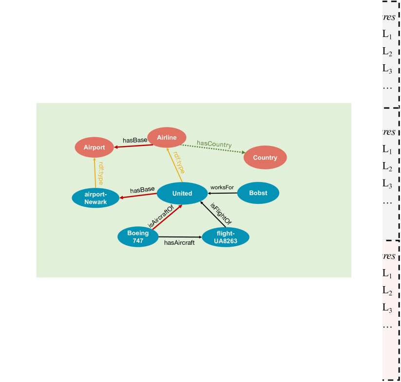
Figure 1. Comparison of different prompt generation paradigms. a The paradigm of using the prompt with fixed templates (Schick and Schütze, 2021; Radford et al., 2021). b The learning paradigms of recent benchmark works, including two major categories: the upper paradigm adopts a certain number of updatable tokens to generate adaptive prompts, and the tokens are learned during training (Zhou et al., 2021; Rao et al., 2021); the lower paradigm uses the same prompt with fixed templates as in a, but further injects an adapter after the fixed text encoder of the pre-trained vision-language model, and the adapter is trainable during inference (Gao et al., 2021; Rao et al., 2021). c The learning paradigm of our method, which directly learn a prompt from the labels by leveraging the effective semantic information from an ontological knowledge graph.

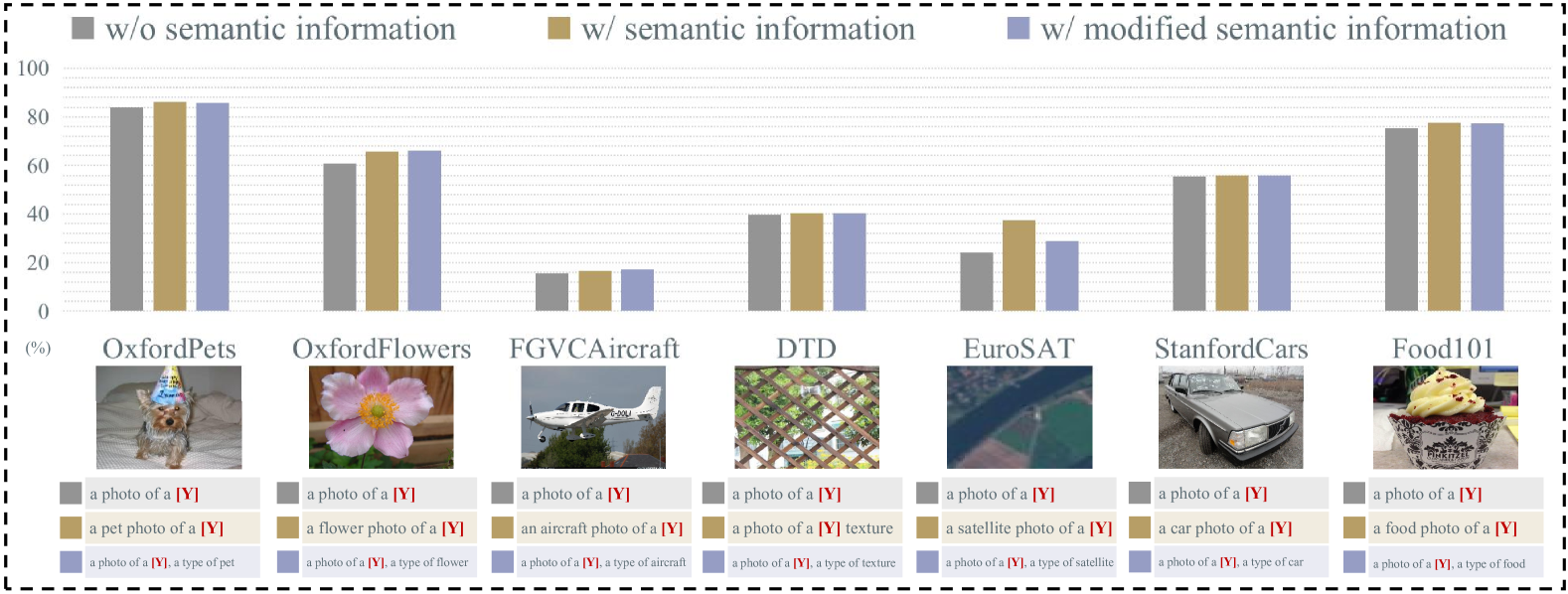
Figure 2. Comparison of different prompt forms for CLIP. We conduct zero-shot inference experiments and the results are shown in the histogram, where grey bars denote the prompt without semantic information which is used by CLIP, brown bars denote the prompt with simple coarse-grained semantic information, and purple bars denote the prompt using more words to describe similar semantic information. We observe that both semantic prompt and longer semantic prompt further improve the performance of CLIP, while the improvement of longer semantic prompt over semantic prompt is limited, which proves that the improvement of CLIP’s performance relies on the addition of semantic information rather than simply adding more words.

As a promising alternative for visual representation learning, vision-language pre-training methods, e.g., CLIP (Radford et al., 2021) and ALIGN (Jia et al., 2021), jointly learn image and text representations with two modality-specific encoders by aligning the corresponding image-text pairs, which is achieved by adopting contrastive loss in pre-training. Benefiting from pre-training on large-scale data, models learn numerous visual concepts so that the learned representations have a strong generalization and can be transferred to various downstream tasks.

(Zhou et al., 2021) observes that the zero-shot generalization performance of the pre-trained vision-language model heavily relies on the form of the text input. Feeding pure labels, i.e., textual names of categories, into the text encoder leads to degenerate performance. To tackle this issue, recent works adopt various prompts to augment the textual labels (Radford et al., 2021; Jia et al., 2021; Schick and Schütze, 2021; Shin et al., 2020; Jiang et al., 2020; Zhou et al., 2021). In the inference stage, the classification weights, i.e., textual label features, are obtained by providing the text encoder with prompts describing candidate categories. The image feature generated by the image encoder is compared with these label features for zero-shot classification.

We conclude the typical prompt generation paradigms in Figure 1. The paradigm, shown in Figure 1 a, rigidly applies the fixed prompt template, which suffers from a dilemma that a specific prompt template has inconsistent boosts for different tasks. A motivating example, proposed by (Zhou et al., 2021), shows that using “a photo of a [Y]” as a prompt for CLIP achieves an accuracy of 60.86% on OxforfFlowers (Nilsback et al., 2008), and using a more describing prompt, i.e., “a flower photo of a [Y]”, can improve the performance to 65.81%, where “[Y]” presents the label text. However, such an improvement is reversed on Caltech101 (Li et al., 2004), where the accuracy of using “a [Y]” is 82.68%, while using “a photo of [Y]” only achieves 80.81%.

To tackle this dilemma, several works (Zhou et al., 2021; Rao et al., 2021; Gao et al., 2021; Rao et al., 2021) explore adopting learnable prompts as shown in Figure 1 b. Generally, these methods rely on the empirical risk loss to optimize the learnable prompt. Both the meaning of the learned prompts and why they work remain unclear. We attribute this in part to the fact that the semantic information of text labels is not explicitly explored, and argue that the label-related semantic information is critical for improving the performance of pre-trained models. Taking CLIP as an example, in the pre-training stage, the original text input of CLIP usually contains rich semantic information, e.g., “a [husky] with black and white hair pulls a sled on the snow” but prompts generated by current methods differ with the training data of CLIP significantly due to the lack of semantic information. To further confirm our hypothesis, we conduct a motivating comparison. Figure 2 demonstrates that prompts with additional semantic information boost the performance of CLIP on all downstream tasks.

To this end, we propose an innovative knowledge-aware prompt learning approach for pre-trained vision-language models, namely, Causality-pruning Knowledge Prompt (CapKP). As illustrated in Figure 1 c, CapKP explores the semantic information associated with the label text by using labels as queries to retrieve an ontological knowledge graph. In practice, we observe that some derived knowledge is redundant for downstream tasks, which may degenerate the performance of our method. Therefore, CapKP introduces causality-pruning to refine the derived label-related knowledge subgraph following the first principle of Granger causality (Granger, 1969). Empirically, CapKP outperforms the state-of-the-art methods, and the transferability comparison supports that CapKP demonstrates stronger robustness than the benchmark methods to domain shifts.

Contributions. The contributions of this paper are four-fold:

• We present a motivating study on the prompt engineering approaches for pre-trained vision-language models in downstream applications and identify the importance of exploring the semantic information of label texts.

• For effectively mining semantic information from the label text, we propose Causality-pruning Knowledge Prompt, which derives label-related semantic information by retrieving an ontological knowledge graph.

• Following the first principle of Granger causality, we propose a causality-pruning method to remove task-redundant information from the label-related knowledge subgraph.

• Empirically, we impose comprehensive comparisons to prove the effectiveness and generalization of our method.

2. Related Work

2.1. Vision-Language Models

Recent development of joint learning on vision and language representations achieves impressive success in various fields, including Visual Question Answering (Anderson et al., 2018; Antol et al., 2015; Gao et al., 2019; Kim et al., 2018), Image Captioning (Huang et al., 2019; You et al., 2016), etc. A critical issue is that few high-quality annotated multi-modal data is available. Therefore, state-of-the-art vision-language models are designed to be pre-trained on massive unannotated data by taking advantage of Transformer (Vaswani et al., 2017), e.g., ViLBERT (Lu et al., 2019), LXMERT (Tan and Bansal, 2019), UNITER (Chen et al., 2019) and Oscar (Li et al., 2020). Such large-scale pre-trained vision-language models have great potential for learning universal representations and transferring them to various downstream tasks via prompting (Jia et al., 2021; Zhang et al., 2020). A representative approach is CLIP (Radford et al., 2021), which pre-trains modality-specific encoders from 400 million image-text pairs and achieves impressive performance in zero-shot inference to multitudinous downstream tasks.

2.2. Prompt Design

Since directly applying pre-trained models to downstream tasks often leads to degenerate performance, CLIP (Radford et al., 2021) and PET (Schick and Schütze, 2021) convert the labels of the downstream task into a batch of manual prompt templates. AutoPrompt (Shin et al., 2020) proposes to automatically search prompts from a template library. (Jiang et al., 2020) proposes two approaches for building the prompt templates, including mining-based and paraphrasing-based approaches. However, such template-based prompting has a critical issue that despite the large-scale candidate template library, the optimal prompt may be excluded.

To perform effective and data-efficient improvement on downstream tasks, simple yet effective adapter-based approaches are proposed, which insert the extra learnable neural network, i.e., adapter, into the large pre-trained models and then train the adapter on downstream tasks under the premise of freezing the weights of the backbone, e.g., Adapters (Houlsby et al., 2019), CLIP-Adapter (Gao et al., 2021) and Tip-Adapter (Zhang et al., 2021). The adapter-based approach can be treated as a post-model prompting, which focuses on improving the performance in the inference stage by re-training adapters, but such an approach does not explore the latent visual concept knowledge learned by the vision-language model in the pre-training stage, which is contrary to the fundamental idea behind prompting, i.e., making the vision-language model recall the pre-trained knowledge relevant to the current downstream task. CoOp (Zhou et al., 2021) and DenseCLIP (Rao et al., 2021) are proposed to automatically learn prompts without the template library, which aim to generate prompts that can make the vision-language model recall the task-relevant knowledge. These methods do not explore the semantic information of the label text in the inference stage, while in this paper we prove the importance of including the label-relevant semantic information in prompting and hence propose to derive such information by leveraging an ontological knowledge graph.

2.3. Knowledge Graph

Knowledge graph abstracts the knowledge in the real world into triples, e.g., <entity, relationship, entity>, to form a multilateral network of relationships, where nodes represent entities and the edges connecting nodes represent the relationships between entities. Knowledge graphs include general domain knowledge graphs, e.g., Wikidata (Vrandecic and Krötzsch, 2014), NELL (Carlson et al., 2010), CN-dbpedia (Xu et al., 2017), ConceptNet (Speer et al., 2017), etc., and specific domain knowledge graphs, e.g., Open PHACTS (Harland, 2012), Watson (Ferrucci et al., 2010), AMiner (Tang et al., 2008), etc. Specifically, ontological knowledge graphs (Geng et al., 2021) only have the ontology entities, i.e., conceptual types, for instance, Wikidata-ZS and NELL-ZS (Qin et al., 2020). To understand the graph-based information from knowledge graphs, Graph embedding (Goyal and Ferrara, 2018; Wang et al., 2017; Glorot et al., 2013; Socher et al., 2013) is proposed, which maps the high-dimensional graph data into the low-dimensional vector, e.g., TransE (Bordes et al., 2013), TransR (Lin et al., 2015), RESCAL (Nickel et al., 2011), KG-BERT (Yao et al., 2019). To mine graph structure information, Graph Neural Network (GNN) based methods are proposed, e.g., KGCN (Wang et al., 2019b). For our approach, we refine the knowledge graph by considering graph causality to eliminate redundant information.

2.4. Graph Causality

In system identification, clarifying the causal relationship between variables by observing the data is a crucial research field. Granger causality (Granger, 1969) is widely used in many fields, e.g., neural network (Kaminski et al., 2001), financial economy (Kónya, 2006), and medicine (Nagarajan and Upreti, 2008). Graph structure has a strong ability to incorporate prior knowledge so graph-based approaches have become crucial tools (Dahlhaus, 2000; Oxley et al., 2009) for analyzing the complex relationships of various interactions among system variables. For understanding the high-dimensional and heterogeneous graph system (Lin et al., 2020; Zitnik et al., 2018; Zitnik and Leskovec, 2017), recent works adopt GNN to learn a graph representation. However, due to the lack of explicit declarative knowledge representation, such methods are regarded as black boxes. Obtaining the graph causality improves the model to mine the latent semantic information of the graph. (Dahlhaus and Eichler, 2003) proposes to study the Granger causality among variables in a graph, which is extended by (Eichler, 2007, 2008). From the perspective of causality, Gem (Lin et al., 2021) understands the behavior of GNN by following Granger causality and describes the causal relationship between each node and the output by splitting local subgraphs.

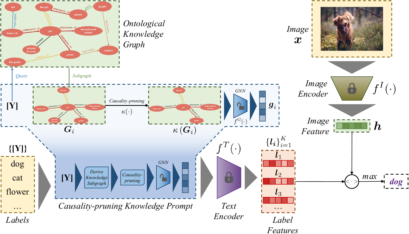
Figure 3. The architecture of Causality-pruning Knowledge Prompt (CapKP). The intuition behind our method is to directly learn a prompt with label-related semantic information rather than adopting a fixed prompt template, which is achieved by introducing refined knowledge from an external knowledge graph. To this end, CapKP consists of two stages: 1) ontology-enhanced knowledge embedding derives the label-related subgraph from an ontological knowledge graph by using the label token as a query; 2) causality-pruned graph representation removes causally irrelevant edges and nodes.

3. Preliminaries

3.1. Vision-Language Pre-training

CLIP (Radford et al., 2021) introduces a pre-training approach to learn semantic knowledge from large amounts of image-text data.

3.1.1. Architecture

CLIP consists of an image encoder and a text encoder. The image encoder aims to learn a high-dimensional representation from an image, which can be implemented by a ResNet (He et al., 2016) or a ViT (Dosovitskiy et al., 2021). The text encoder aims to learn a text representation from a sequence of words, which is implemented by a Transformer (Vaswani et al., 2017).

3.1.2. Training

For texts, all tokens (words and punctuations) are mapped into lower-cased byte pair encoding representations (Sennrich et al., 2016). They are further projected into vectors with 512 dimensions, which are then fed to the text encoder. The input sequence of the text encoder is capped at a fixed length of 77. The input images are encoded into the embedding space by the image encoder. CLIP is trained from an excessively large-scale unsupervised dataset consisting of 400 million image-text pairs by aligning the two embedding spaces for images and texts, respectively. The learning objective is formulated as a contrastive loss (Chen et al., 2020). The learned text and image representations have strong generalization capability for various downstream tasks.

3.1.3. Inference

CLIP performs zero-shot image recognition as downstream tasks by measuring the similarity of image features with the label features generated by the text encoder, which takes as input the relevant textual descriptions of the specified categories. Suppose $\bm{h}$ denotes the image features extracted by the image encoder $f^{I}(\cdot)$ for an image $\bm{x}$ and $\left\{\bm{l}_{i}\right\}_{i=1}^{K}$ denotes a set of label features extracted by the text encoder $f^{T}(\cdot)$ from prompts $\left\{\bm{p}_{i}\right\}_{i=1}^{K}$ with a form of “a photo of a [Y].”, where $K$ is the number of classes, and [Y] presents a specific class name, e.g., “dog”, “cat”, or “flower”. The prediction probability is computed by

(1) $${\mathcal{P}}\left(y=i|\bm{h}\right)=\frac{{\exp\left(\frac{<\bm{l}_{i},\bm{h}>}{\tau}\right)}}{\sum_{j=1}^{K}{\exp\left(\frac{<\bm{l}_{j},\bm{h}>}{\tau}\right)}}.$$

where $y$ denotes the semantically correct category for $\bm{x}$, $\tau$ is the temperature hyper-parameter in CLIP, and $<\cdot,\cdot>$ denotes the cosine similarity. Compared with the conventional classifier learning approach where only closed-set visual concepts can be classified, the zero-shot inference paradigm of vision-language pre-training models can explore open-set concepts with the text encoder.

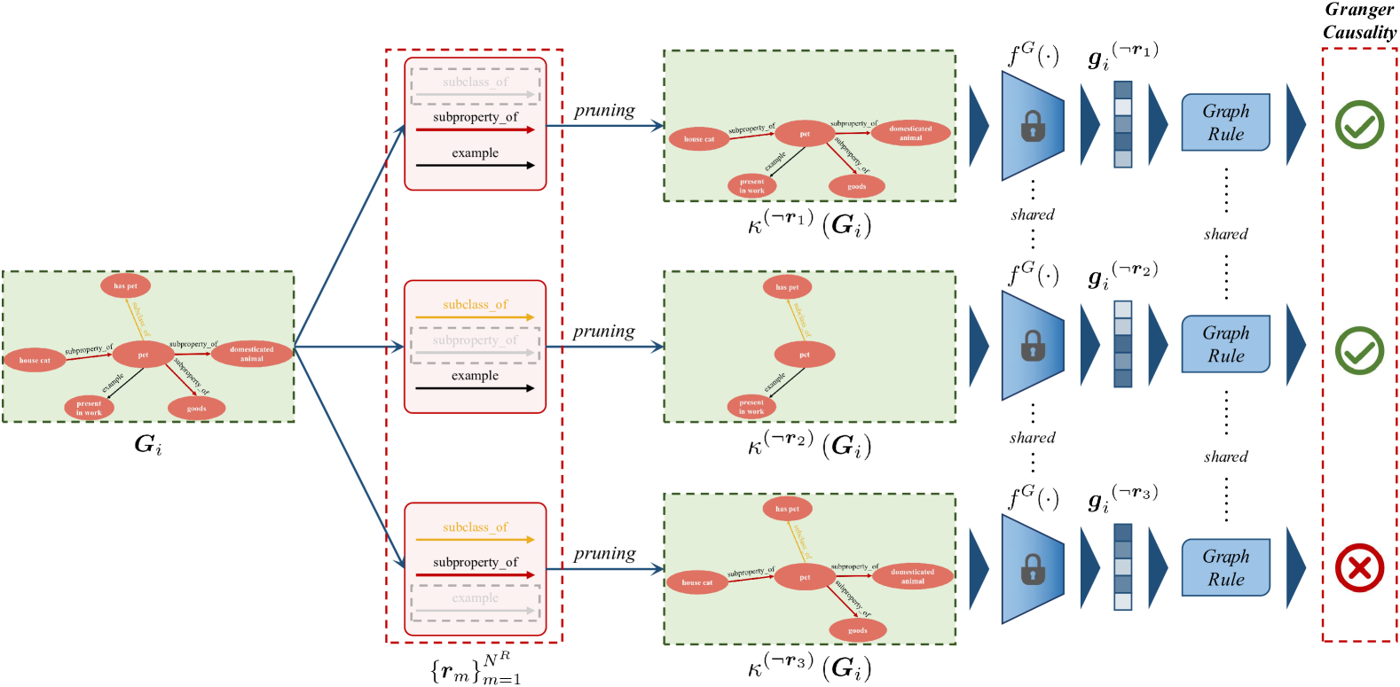
Figure 4. An example of the rationale of causality-pruned graph representation. Following the first principle of Granger causality, we refine the derived knowledge subgraph $\bm{G}_{i}$ by pruning the edges that are causally decoupled from the downstream task. We determine the Granger causality by iteratively removing the edges related to a relation-type $\bm{r}_{m}$ and then checking the oscillation of the result, which is computed by following a specific graph rule. Only causally related edges are kept and others are pruned. Note that the graph encoder $f^{G}\left(\cdot\right)$ is fixed throughout the process.

3.2. Graph Representation Learning

3.2.1. Graph Setup

We recap necessary preliminaries of graph representation learning. Let $\bm{G}=(\bm{V},\bm{E})$ be an attributed graph, where $\bm{V}$ is the node set and $\bm{E}$ is the edge set. Given a graph dataset $\mathcal{G}={\bm{G}_{i},i\in\llbracket{1,N^{G}}\rrbracket}$, where $\bm{G}_{i}$ is sampled i.i.d from the distribution $\mathcal{P}\left(\mathcal{G}\right)$, the objective of graph representation learning is to learn an encoder $f^{G}(\cdot):\mathcal{G}\to\mathbb{R}^{d^{G}}$, where $\mathbb{R}^{d^{G}}$ denotes a $d^{G}$-dimensional embedding space and $f^{G}(\bm{G}_{i})$ is the representation of $\bm{G}_{i}$.

3.2.2. Graph Neural Network

Most benchmark methods employ GNN as the encoder. GNN encodes each node in $\bm{G}_{i}=(\bm{V}_{i},\bm{E}_{i})$ into a representation vector, where $\bm{H}_{\bm{v}}$ denotes the representation vector for node $\bm{v}\in\bm{V}_{i}$. The $k$-th layer of GNN can be formulated as:

(2) $$\bm{H}^{\left(k+1\right)}_{\bm{v}}=COMBINE^{\left(k\right)}\Bigg{(}\bm{H}^{\left(k\right)}_{\bm{v}},AGG^{\left(k\right)}\left(\bm{H}^{\left(k\right)}_{\bm{u}},\forall\bm{u}\in\mathcal{N}\left(\bm{v}\right)\right)\Bigg{)},$$

where $\mathcal{N}\left(\bm{v}\right)$ denotes the neighbors of $\bm{v}$, $\bm{H}^{\left(k\right)}$ is the representation vector of the corresponding node at the $k$-th layer. For the $0$-th layer, $\bm{H}^{\left(0\right)}$ is initialized with the input node feature. $COMBINE$ and $AGG$ are learnable functions of GNN, where $AGG$ aggregates the features of neighbours and $COMBINE$ combines the aggregated neighbour feature into the feature of the target node. After several rounds of massage passing, a readout function pools the node representations $\left\{\bm{H}_{\bm{v}}|\bm{v}\in\bm{V}_{i}\right\}$ to obtain the graph representation $\bm{g}_{i}$ for $\bm{G}_{i}$:

(3) $${\bm{g}_{i}}=READOUT\left(\bm{H}_{\bm{v}},\bm{v}\in\bm{V}_{i}\right).$$

4. Methodology

From the experiments in Figure 2, we conclude a common assumption for prompting pre-trained vision-language models:

Assumption 4.1.

(Semantic information in prompts). Introducing label-relevant semantic information in prompts boosts the performance of the pre-trained vision-language model in downstream zero-shot inference tasks.

Holding Assumption 4.1, we propose an innovative approach, namely CapKP, to effectively add label-relevant semantic information in prompts. The overall architecture of CapKP is illustrated in Figure 3. We empower the proposed CapKP by two designs: ontology-enhanced knowledge embedding and causality-pruned graph representation.

4.1. Learnable Knowledge Prompt

To perform the learnable prompt, we replace the original input of CLIP’s text encoder, i.e., the lower-cased byte pair encoding representation, with the representation learned by CapKP.

4.1.1. Label-specific prompt

We generate the label-specific prompt set $\left\{\bm{p}_{i}\right\}_{i=1}^{K}$ by

(4) $${\bm{p}_{i}=\left(\bm{\mu}+\lambda\cdot\varphi\left(\bm{[Y]}_{i}\right)\right)\oplus b\left(\bm{[Y]}_{i}\right)},$$

where $\bm{\mu}$ is a set of learnable feature vectors, which are randomly initialized by Gaussian distributions. $\varphi\left(\cdot\right)$ denotes the function of our proposed CapKP, and $\lambda$ is the coefficient that controls the balance between $\bm{\mu}$ and $\varphi\left(\cdot\right)$. $b\left(\bm{[Y]}_{i}\right)$ denotes the lower-cased byte pair encoding representation of label $\bm{[Y]}_{i}$, and $\oplus$ is a concatenation function. Note that the output of $\varphi\left(\cdot\right)$ is a vector with the same dimension as $b\left(\bm{[Y]}_{i}\right)$, e.g., 512 for CLIP. Feeding prompts $\left\{\bm{p}_{i}\right\}_{i=1}^{K}$ to the text encoder $f^{T}\left(\cdot\right)$, we obtain the classification weights $\left\{\bm{l}_{i}\right\}_{i=1}^{K}$, and the prediction probability is computed by Equation 1.

4.1.2. Label-shared prompt

From the perspective of revisiting the training data for the vision-language model, we observe that the input text does not focus on describing the label-specific and discriminative semantic information; on the contrary, words with semantic information shared by different labels appear in a large body of descriptive text. For the examples “a [golden retriever] runs on the grass with its tail wagging” and “an [Alaskan] sits on a couch with a floppy tail”, there only exists the label-shared information, i.e., “tail”, but no label-specific information. Such a phenomenon is common in the description of fine-grained labels, and we thus hold an extended assumption:

Assumption 4.2.

(Generalized semantic information in prompts). Label-specific semantic information could be task-redundant to prompt pre-trained vision-language models, while generalized label-shared semantic information is crucial for generating effective prompts.

See Section 5 for the experimental proof for Assumption 4.2. We thus propose a label-shared prompt form by

(5) $${\bm{p}_{i}=\left(\bm{\mu}+\lambda\cdot\psi\left(\left\lfloor\left\{\varphi\left(\bm{[Y]}_{j}\right)\right\}_{j=1}^{K}\right\rceil\right)\right)\oplus b\left(\bm{[Y]}_{i}\right)},$$

where $\left\lfloor\cdot\right\rceil$ presents a cascade concatenation function, detailed by $\left\lfloor\left\{\varphi\left(\bm{[Y]}_{j}\right)\right\}_{j=1}^{K}\right\rceil=\varphi\left(\bm{[Y]}_{1}\right)\oplus\varphi\left(\bm{[Y]}_{2}\right)\oplus\ldots\oplus\varphi\left(\bm{[Y]}_{K}\right)$, and $\psi\left(\cdot\right)$ presents a linear mapping function in CapKP.

4.2. Ontology-enhanced Knowledge Embedding

We propose to retrieve an ontological knowledge graph by treating an input label as the query and further capture the corresponding high-order knowledge representation through a GNN. Given a input label $\bm{[Y]}_{i}$, we start by locating the 1-hop label-relevant subgraph $\bm{G}_{i}$, which is performed by obtaining the knowledge graph entity with the largest semantic similarity to $\bm{[Y]}_{i}$ and retrieving all neighbor entities that are directly connected to it by an edge. We then refine the subgraph by causality-pruning to remove redundant information and encode the pruned subgraph into a vector by the function $\varphi\left(\cdot\right)$ in Equation 4 and Equation 5, which is defined by

(6) $$\varphi\left(\bm{[Y]}_{i}\right)=\bm{g}_{i}=f^{G}\left(\kappa\left(\bm{G}_{i}\right)\right)$$

where $\kappa\left(\cdot\right)$ denotes the proposed causality-pruning function, and $f^{G}\left(\cdot\right)$ is implemented by GNN. To explore the structural proximity among entities in a knowledge graph, we impose $AGG\left(\cdot\right)$ in GNN by following (Wang et al., 2019b). Suppose $\bm{v}$ denotes the label-related entity (node), and $\bm{e}_{\bm{v},\bm{u}}$ denotes a relation (edge) between entities $\bm{v}$ and $\bm{u}$. $AGG\left(\cdot\right)$ is implemented by

(7) $$\widehat{AGG}\left(\bm{v}\right)=MLP\left(\bm{H}_{\bm{v}}+\sum_{\bm{u}\in\widetilde{\mathcal{N}}\left(\bm{v}\right)}\frac{\exp\left(<\bm{H}_{\bm{v}},\bm{H}_{\bm{e}_{\bm{v},\bm{u}}}>\right)}{\mathop{\sum}\limits_{\bm{u}^{\prime}\in\widetilde{\mathcal{N}}\left(\bm{v}\right)}\exp\left(<\bm{H}_{\bm{v}},\bm{H}_{\bm{e}_{\bm{v},\bm{u}^{\prime}}}>\right)}\bm{H}_{\bm{u}}\right)$$

where $MLP$ denotes a non-linear network, $\bm{H}$ denotes the corresponding representation for a node or an edge, $<\cdot,\cdot>$ is a inner-product function, and $\widetilde{\mathcal{N}}\left(\bm{v}\right)$ is the neighborhood set of $\bm{v}$ in the causality-pruned graph $\kappa\left(\bm{G}_{i}\right)$.

4.3. Causality-pruned Graph Representation

To describe our intuition of causality-pruning, we reform the definition of Granger causality (Granger, 1969) in the field of knowledge graph:

Definition 4.3.

(Granger causality in knowledge graph). Granger causality (Granger, 1969; Granger and W., 1980) describes the relationships between two (or more) variables when one is causing the other. In the field of the knowledge graph, if we are better able to predict variable $\Upsilon$, e.g., higher score computed by a specific graph rule, using all available information $\Omega$ than if the information apart from a variable $\chi$, e.g., a type of relation, had been used, we say that $\chi$ Granger-causes $\Upsilon$ (Granger and W., 1980).

Given the label-relevant knowledge subgraph $\bm{G}_{i}$ and the set of relation-types in the retrieved ontological knowledge graph $\left\{\bm{r}_{m}\right\}_{m=1}^{N^{R}}$, we aim to remove the relation-types that are decoupled from predicting $\bm{G}_{i}$ according to Granger causality. To this end, we capture the individual causal effect, proposed by (Goldstein et al., 2015; Lin et al., 2021), of the knowledge subgraph $\bm{G}_{i}$ with the relation-type $\bm{r}_{m}$ on $\bm{l}_{i}$.

We demonstrate causality-pruned graph representation in Figure 4, where Graph Rule denotes the process of quantitatively computing a score to ascertain whether Granger causality holds between a specific pruned relation-type and predicting the graph. Following Definition 4.3 and the proposed Graph Rule, we quantify the causal contribution of a relation-type $\bm{r}_{m}$ to the output of final $f^{T}\left(\cdot\right)$ by measuring the reduction in joint model error, formulated as:

(8) $$\varDelta_{\epsilon,\bm{r}_{m}}=\epsilon_{\kappa^{\left(\neg\bm{r}_{m}\right)}\left(\bm{G}_{i}\right)}-\epsilon_{\bm{G}_{i}}$$

where $\epsilon_{\bm{G}_{i}}$ denotes the joint model error of the $f^{G}\left(\cdot\right)$ and $f^{T}\left(\cdot\right)$ when considering the computation graph, and $\epsilon_{\kappa^{\left(\neg\bm{r}_{m}\right)}\left(\bm{G}_{i}\right)}$ denotes the joint model error excluding the relation-type $\bm{r}_{m}$. We determine the Granger causality between $\bm{r}_{m}$ and predicting the graph by

(9) $$\begin{cases}\bm{r}_{m}\ \ \ Granger-causes\ \ \ \Upsilon,&\quad\varDelta_{\epsilon,\bm{r}_{m}}>0\\ \bm{r}_{m}\ \ \ \textit{NOT}\ \ \ Granger-causes\ \ \ \Upsilon,&\quad\varDelta_{\epsilon,\bm{r}_{m}}\leq 0\end{cases}$$

where $\Upsilon$ represents a supposed fact that the specific relation-type helps the model to predict the graph and further improve the text representation $\bm{l}_{i}$ learned by the joint model, i.e., $f^{G}\left(\cdot\right)$ and $f^{T}\left(\cdot\right)$.

  Input: The annotated images datasets $X^{tr}$ and $X^{te}$ for the training and test phases of few-shot learning, respectively. The corresponding label set $\left\{\bm{[Y]}_{j}\right\}_{j=1}^{K}$. Minibatch size $n$. Coefficient $\lambda$.

  Initialize The learnable neural network parameters: ${\theta}$ for the graph encoder $f_{\theta}^{G}(\cdot)$ and ${\vartheta}$ for the learnable feature vectors $\bm{\mu}$, which share a learning rate $\ell$. The fixed pre-trained parameters for the text encoder $f^{T}(\cdot)$ and the image encoder $f^{I}(\cdot)$.

  repeat

     $\#\ training\ phase\ of\ few-shot\ learning$

     for $t$-th training iteration do

        Sample a minibatch $\bar{X}^{tr},\bar{Y}^{tr}=\left\{\bm{x}_{i},\bm{y}_{i}\right\}_{i=(t-1)n}^{tn}\in X^{tr}$.

        $\#\ generate\ label\ features\ without\ causality-pruning$

        $\left\{\bm{l}_{j}\right\}_{j=1}^{K}=\left(\bm{\mu}_{\vartheta}+\lambda\cdot f^{T}\left(f^{G}_{\theta}\left(\bm{G}_{j}\right)\right)\oplus b\left(\bm{[Y]}_{j}\right)\right)$

        $\theta\leftarrow\theta-\ell\cdot\Delta_{\theta}\mathcal{L}_{cross-entropy}(\left\lfloor\left\{<\bm{l}_{j},f^{I}\left(\bar{X}^{tr}\right)>\right\}_{j=1}^{K}\right\rceil,\bar{Y}^{tr})$

        $\vartheta\leftarrow\vartheta-\ell\cdot\Delta_{\vartheta}\mathcal{L}_{cross-entropy}(\left\lfloor\left\{<\bm{l}_{j},f^{I}\left(\bar{X}^{tr}\right)>\right\}_{j=1}^{K}\right\rceil,\bar{Y}^{tr})$

     end for

  until $\theta$ converges.

  $\#\ test\ phase\ of\ few-shot\ learning$

  for $t$-th test iteration do

     Sample a minibatch $\bar{X}^{te},\bar{Y}^{te}=\left\{\bm{x}_{i},\bm{y}_{i}\right\}_{i=(t-1)n}^{tn}\in X^{te}$.

     $\#\ generate\ label\ features\ with\ causality-pruning$

     $\left\{\bm{l}_{j}\right\}_{j=1}^{K}=\left(\bm{\mu}_{\vartheta}+\lambda\cdot f^{T}\left(f^{G}_{\theta}\left(\kappa\left(\bm{G}_{j}\right)\right)\right)\oplus b\left(\bm{[Y]}_{j}\right)\right)$

     $Y^{predict}=\mathop{\max}\limits_{j}\left\{<\bm{l}_{j},f^{I}\left(\bar{X}^{tr}\right)>\right\}_{j=1}^{K}$

  end for

Algorithm 1 CapKP(SPE)

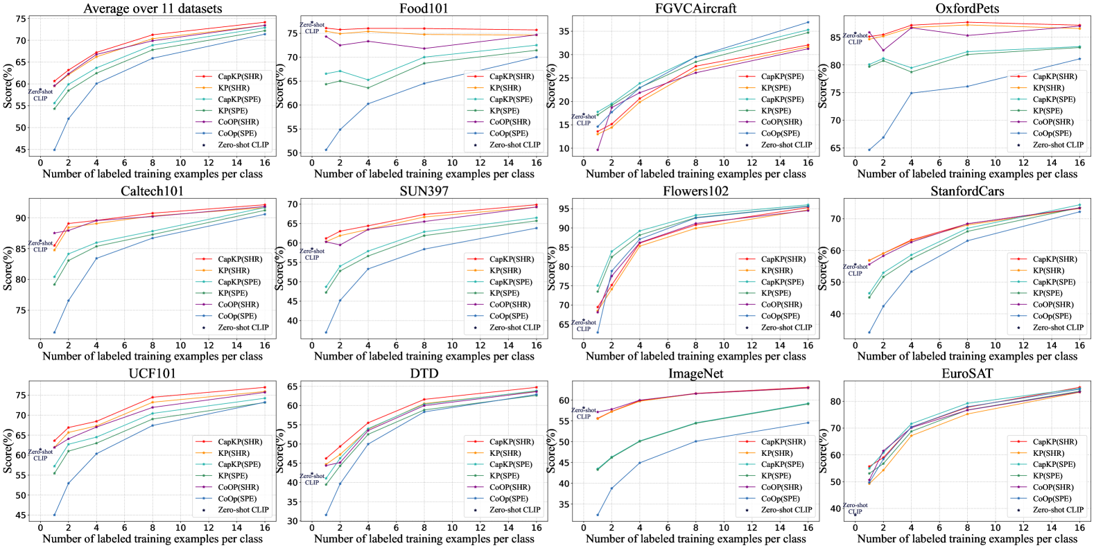
Figure 5. Comparisons of few-shot learning on 11 datasets. CapKP consistently outperforms baselines within different shots.

Table 1. Comparisons of CapKP with CoOp. Both models are trained on 11 benchmark datasets within 8 shots. CapKP outperforms CoOp on most datasets. $\triangle$ denotes CapKP’s gain over CoOp.

	OxfordPets	Flowers102	FGVCAircraft	DTD	EuroSAT	StanfordCars	Food101	SUN397	Caltech101	UCF101	ImageNet	Average
CoOp	85.32	91.18	26.13	59.97	76.73	68.43	71.82	65.52	90.21	71.94	61.56	69.89
CapKP	87.72	90.81	27.54	61.58	77.79	68.40	76.00	67.34	90.75	74.47	61.63	71.28
$\triangle$	2.40	-0.37	1.41	1.61	1.06	-0.03	4.18	1.82	0.54	2.53	0.07	1.39

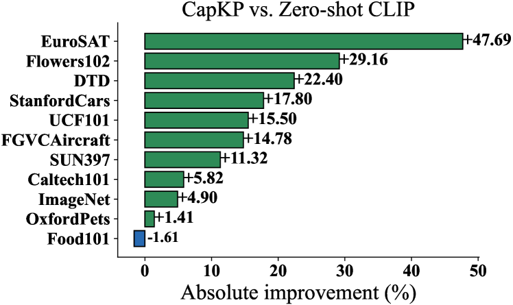
Figure 6. Comparisons with CapKP and CLIP.

4.4. Variants of Our Method

Our complete method is called CapKP. We perform an ablation study by eliminating the module of causality-pruning and deriving a variant KP. Considering two forms of prompts that are discussed in Section 4.1.1 and Section 4.1.2, we abbreviate label-specific prompt and label-shared prompt as SPE and SHR, respectively.

4.5. Algorithm pipline

In the inference stage, we train and evaluate our method by following the benchmark-setting (Zhou et al., 2021). It is worth noting that we only adopt causality-pruned graph representation in the test phase of few-shot learning. We take CapKP(SPE) as an example to demonstrate the pipeline in Algorithm 1.

5. Experiments

5.1. Few-Shot Learning

5.1.1. Datasets

We conduct experiments on 11 publicly available image classification datasets: ImageNet (Deng et al., 2009), Caltech101 (Li et al., 2004), StandfordCars (Krause et al., 2013), FGVCAircraft (Maji et al., 2013), Flowers102 (Nilsback et al., 2008), OxfordPets (Parkhi et al., 2012), Food101 (Bossard et al., 2014), SUN397 (Xiao et al., 2010), UCF101 (Soomro et al., 2012), DTD (Cimpoi et al., 2014), and EuroSAT (Helber et al., 2019). These datasets cover general object classification tasks, scene recognition tasks, action recognition tasks, fine-grained classification tasks, and specialized tasks such as texture recognition and satellite image recognition, which constitute a comprehensive benchmark. Following the principle of CLIP (Radford et al., 2021) and CoOp (Zhou et al., 2021), we train our model with 1, 2, 4, 8, and 16 shots, respectively, and evaluate it in test sets. The average results over three runs are reported.

5.1.2. Baselines

We compare our approach with two major baseline models: 1) CLIP (Radford et al., 2021), which is based on manual prompts, and we follow the instructions for prompt ensembling in (Radford et al., 2021) and input seven corresponding prompt templates into the CLIP text encoder; 2) CoOp (Zhou et al., 2021), which automatically designs the prompt templates, and for fair comparisons, we adopt the best variants of CoOp.

5.1.3. Training Details

The set of learnable feature vectors $\bm{\mu}$ is randomly initialized by zero-mean Gaussian distributions with a standard deviation of 0.02. According to the parameter study in Appendix A, we assign the coefficient $\lambda$to $10^{-2}$. We set the maximum epoch to 200, 100, and 50 for 16/8 shots, 4/2 shots, and 1 shot, respectively, while the maximum epoch on ImageNet is fixed to 50 for all shots. Unless otherwise specified, ResNet-50 (He et al., 2016) and Transformer (Vaswani et al., 2017) are used as the corresponding image and text encoders. We initially adopt Wikidata-ZS (Qin et al., 2020) as the target ontological knowledge graph, while we also conduct experiments to evaluate our method using Nell-ZS (Qin et al., 2020) in Appendix B.

Table 2. Visualization of feature vectors $\bm{\mu}$ with the length of 16 learned by CapKP(SHR). We derive the words by measuring the Euclidean distances between word embeddings and each specific feature vector of $\bm{\mu}$, and the quantified distances are shown in parentheses. N/A represents non-Latin characters. The task-relevant words are marked in BOLD.

#	ImageNet	Food101	OxfordPets	DTD	UCF101
1	where (1.4992)	winery (1.0086)	vac (1.2409)	himss (1.1484)	ditch (1.2119)
2	N/A (1.2287)	grain (1.2845)	o (1.2407)	essential (0.9013)	peek(1.2222)
3	a (1.4260)	gra (0.9716)	sav (1.1540)	dw (1.5142)	tolerate (0.9314)
4	allow (1.5591)	N/A (0.9465)	rous (0.9295)	thats (1.1830)	photo (1.3124)
5	thepersonalnetwork(1.5642)	wonder(1.4191)	mo(0.8267)	**** (1.6619)	thinkin(1.4635)
6	inadequate(1.9244)	go(0.8285)	goes(0.8335)	serious(0.6558)	sive(0.9611)
7	humans (1.4764)	artsy (1.2367)	zar (1.2723)	daener (1.3378)	spl (1.8495)
8	hon (1.2362)	valen (1.0958)	autumn (1.4099)	2 (0.7010)	believed (1.6348)
9	inn (1.0578)	ente (1.2312)	/ (1.1853)	N/A (1.4208)	stool (2.0230)
10	for (1.0963)	preparation (1.3788)	firmly (0.9633)	der (1.4271)	swing (1.3811)
11	gi (1.1065)	absol (1.4179)	bles (0.8048)	ett (1.8202)	braving (1.8438)
12	.. (1.5250)	ardu (1.6931)	owner (1.0334)	gs (1.1643)	gent (1.5629)
13	about (1.4677)	struck (1.0167)	compliant (1.2167)	order (1.4104)	visuals (1.4737)
14	oxy (1.7380)	pab (0.6368)	dog (1.0107)	il (1.7677)	shima (1.7922)
15	s (1.7768)	main (1.5293)	scrutiny (1.3651)	phase (1.1731)	south (1.5168)
16	nage (1.6341)	er (0.9222)	enabled (1.1544)	death (0.9549)	par (1.6291)

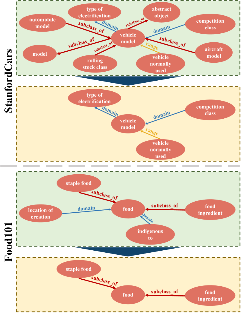
Figure 7. Visualization of Causality-pruning, demonstrating that CapKP removes task-irrelevant relations.

Table 3. Comparisons of CapKP with baselines on robustness to distribution shift using different vision backbones. Both CoOp and CapKP use the shared label prompt, i.e., SHR. M denotes the length of learnable feature vectors $\bm{\mu}$.

Method	Target				Average
	-V2	-Sketch	-A	-R
ResNet-50
Zero-Shot CLIP	51.34	33.32	21.65	56.00	40.58
CoOp (M=16)	55.11	32.74	22.12	54.96	41.23
CoOp (M=4)	55.40	34.67	23.06	56.60	42.43
CapKP(M=16)	55.48	33.10	21.57	54.49	41.16
CapKP(M=4)	55.14	34.75	23.43	57.44	42.69
ResNet-101
Zero-Shot CLIP	54.81	38.71	28.05	64.38	46.49
CoOp (M=16)	58.66	39.08	28.89	63.00	47.41
CoOp (M=4)	58.60	40.40	29.60	64.98	48.39
CapKP(M=16)	58.03	39.78	28.87	63.46	47.54
CapKP(M=4)	59.06	40.80	29.91	65.29	48.77
ViT-B/32
Zero-Shot CLIP	54.79	40.82	29.57	65.99	47.79
CoOp (M=16)	58.08	40.44	30.62	64.45	48.40
CoOp (M=4)	58.24	41.48	31.34	65.78	49.21
CapKP(M=16)	58.56	40.81	30.55	65.83	48.94
CapKP(M=4)	58.75	41.48	31.97	66.66	49.71
ViT-B/16
Zero-Shot CLIP	60.83	46.15	47.77	73.96	57.18
CoOp (M=16)	64.18	46.71	48.41	74.32	58.41
CoOp (M=4)	64.56	47.89	49.93	75.14	59.38
CapKP(M=16)	64.32	46.99	49.13	74.40	58.71
CapKP(M=4)	64.28	48.19	49.29	75.59	59.34

5.1.4. Comparison with Baselines

The experimental results on 11 benchmark datasets are demonstrated in Figure 5, and the average results are shown in the top-left subfigure. We observe that CapKP achieves state-of-the-art results under settings of different shots. With fewer shots, e.g., 1/2/4/8 shots, CapKP improves the baselines by a significant margin. With the increase of shots, each compared method achieves better performance and the performance gap becomes smaller, while CapKP still outperforms benchmark methods. Figure 1 shows the gains obtained by CapKP at 16 shots over the hand-crafted prompt method, i.e., zero-shot CLIP. In specific tasks, e.g., Eurosat, CapKP beats zero-shot CLIP by nearly 50%. In Table LABEL:tab:CoOp, we observe that the improvements of CapKP over CoOp reach 4.18%, 2.40%, and 1.41% on fine-grained image classification datasets, including Food101, OxfordPets, and FGVCAircraft, respectively. CapKP also outperforms CoOp by a significant margin (more than 1%) on scene and action recognition tasks, e.g., UCF101 and SUN397. The effectiveness of KP and CapKP further verifies the proposed Assumption 4.1 and Assumption 4.2, respectively.

5.2. Domain Generalization

5.2.1. Datasets

For domain generalization experiments, we use ImageNet as the source dataset and four variants of ImageNet, i.e., ImageNetV2 (Recht et al., 2019), ImageNet-Sketch (Wang et al., 2019a), ImageNet-A (Hendrycks et al., 2021b) and ImageNet-R (Hendrycks et al., 2021a), as the target datasets. The classes of the variants are subsets of the 1,000 classes of ImageNet, allowing seamless transfer for the prompts learned by CoOp or CapKP.

5.2.2. Results

The results, with various vision backbones, are shown in Table LABEL:tab:rob. CapKP achieves the best performance on most datasets, which demonstrates that our method is generally more robust to distribution shifts than baselines. CapKP(M=4) has better performance than CapKP(M=16), which is tenable and consistent with (Zhou et al., 2021), i.e., using fewer context tokens leads to better robustness.

5.3. Further Analysis

5.3.1. Interpreting the Learned Prompts

We interpret the learned prompt by transforming the learned feature vector into the word closest to the corresponding vector in the hidden space. Table LABEL:tab:word shows the visualized feature vectors of $\bm{\mu}$ on benchmark datasets. We observe that there exist words that are task-relevant, e.g., “winery”, “grain” and “ente” for Food101, “compliant” and “dog” for OxfordPets. From the experimental results demonstrated by (Radford et al., 2021), we observe that CoOp hardly learns task-relevant lexical features, since its training is only based on gradient back-propagation. Concretely, our proposed CapKP empowers the model to learn task-relevant feature vectors with rich semantic information. See Appendix C for further study, which demonstrates that the vectors learned by CapKP(SPE) capture more task-related words.

5.3.2. Visualization of Causality-pruning

We visualize the process of the proposed causality-pruning. Figure 2 illustrates two examples on Food101 and StanfordCars, which show that different relation-types Granger-cause predicting the graph on different datasets. Following the first principle of Granger causality, CapKP can remove several task-irrelevant relations. The results in Figure 5 further support the effectiveness of the proposed causality-pruning.

6. Conclusion

In this paper, we find out the importance of the textual label’s semantic information for prompting the pre-trained vision-language model through empirical observation. To explore such semantic information, we propose CapKP, which complements semantic information for the input label text by leveraging an ontological knowledge graph and further refining the derived label-relevant knowledge subgraph by the proposed causality pruning. We conduct extensive comparisons to prove the superiority of CapKP over benchmark manual prompt methods and learnable prompt methods in few-shot classification and domain generalization.

In this section, we provide several experimental analyses about the advantages of our proposed method. The experiments to find appropriate hyperparameters are conducted as well.

Appendix A Appendix: Parameter Study of $\lambda$

As demonstrated in Figure 8, we report the results of the model with different $\lambda$ values based on Flowers102 at 1 shot. The parameter study is conducted on the validation set. To explore the influence of $\lambda$, we fix other experimental settings and select $\lambda$ from the range of {$10^{-4},10^{-3},10^{-2},0.1,1$}. We can observe that the score reaches the maximum when the $\lambda$ is $10^{-2}$, which indicates that an appropriate tuning of the impact of the knowledge embedding to guide the training of learnable label features, i.e., $\mu$, can indeed promote the performance of CLIP on downstream tasks. While excessively emphasizing the impact of knowledge embedding on training may degenerate the ability of the learnable features $\mu$ to fit appropriate prompts needed for downstream tasks by using gradient back-propagation so that the performance of CLIP is weakened. The setting of $\lambda$ is shared among different downstream tasks.

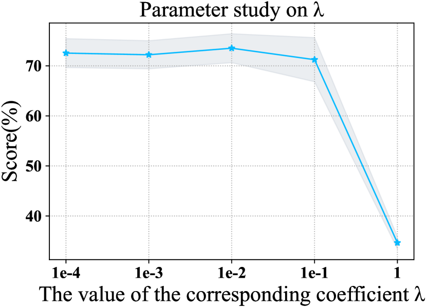
Figure 8. Parameter study on $\lambda$. We choose the best coefficient value of $\lambda$ as 10^-2 in benchmark experiments. The shade denotes the range of experimental results.

Appendix B Appendix: Performing CapKP with Different Knowledge Graphs

As shown in Figure 9, we report the results of the model trained on four datasets at 8 shots using Wikidata-ZS or NELL-ZS ontological knowledge graphs.

We detail the descriptions of the candidate knowledge graphs in Table LABEL:tab:kgdesc. Nell-ZS is constructed based on NELL (Carlson et al., 2010) and Wikidata-ZS is based on Wikidata (Vrandecic and Krötzsch, 2014). Both Nell and Wikidata are large-scaled and another merit is the existence of official relation descriptions. The NELL and Wikidata are two well-configured knowledge graphs and the textual descriptions of Nell-ZS and Wikidata-ZS consist of multiple information.

We observe the results reported in Figure 9 and find that, generally, our model CapKP and the ablation model KP achieve better performance using the Wikidata-ZS knowledge graph compared to using NELL-ZS on several benchmark datasets, e.g., DTD and EuroSAT. We reckon the reason is that Wikidata-ZS has more detailed relations and entities, which empowers our method to locate label-related knowledge subgraphs, yet Nell-ZS does not have sufficient relations and entities so our method may not be able to find knowledge subgraphs corresponding to several specific labels. Such a conclusion is consistent with our proposed Assumption 4.1. However, we further observe that the difference between the performance of our method using Wikidata-ZS and using Nell-ZS is not extremely large on some benchmark datasets, e.g., Food101 and OxfordPets. According to Assumption 4.2, we speculate the reason is that Although Nell-ZS does not contain enough label-related knowledge, it contains sufficient generalized label-related knowledge for certain datasets, for instance, Nell-ZS does not contain the entities of “chocolate” and “potato”, while it contains “concept:food” so that the knowledge subgraph of “concept:food” can be used for amounts of labels. According to Assumption 4.2, the important content of prompts may not contain label-specific and discriminative information, and generalized label-shared semantic information is crucial for generating effective prompts.

In general, both Assumption 4.1 and Assumption 4.2 can be further proved by the experiments in Figure 9.

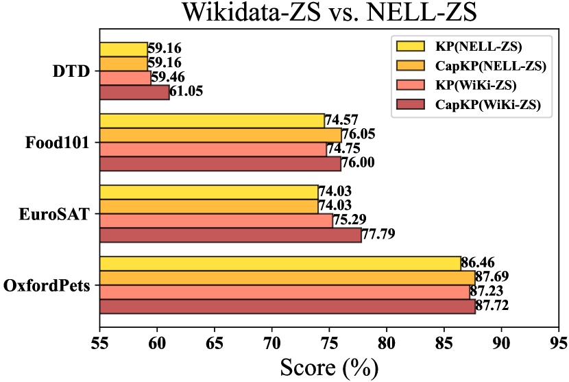
Figure 9. Comparisons of leveraging two different knowledge graphs, i.e., Nell-ZS and Wikidata-ZS (a.k.a., Wiki-ZS).

Table 4. Statistics of the adopted ontological knowledge graphs. # Ent. denotes the number of unique entities. # Triples denotes the amount of relation triples. # Train/Dev/Test denotes the number of relations for training/validation/testing.

Dataset	# Ent.	# Triples	# Train/Dev/Test
Nell-ZS	1,186	3,055	139/10/32
Wiki-ZS	3,491	10,399	469/20/48

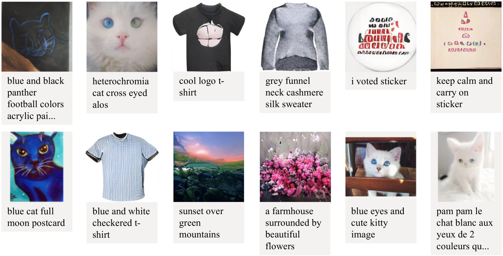
Figure 10. Real-world examples of input pairs for CLIP in the pre-training phase, including descriptive text and images.

Table 5. Visualization of feature vectors $\bm{\mu}$ with the length of 101 learned by CapKP(SPE) on Food101, i.e., a category corresponds to a word. We derive the words by measuring the Euclidean distances between word embeddings and each specific feature vector of $\bm{\mu}$, and the quantified distances are shown in parentheses. N/A represents non-Latin characters.

No.		No.		No.		No.
1	chandelier (0.7779)	2	N/A (0.7436)	3	oured (0.8188)	4	val (0.7030)
5	mises (0.7793)	6	pesto (0.6852)	7	daily (0.6644)	8	vaz (0.5889)
9	ergon (0.7521)	10	watercolor (0.7230)	11	daz (0.6812)	12	baguette (0.6713)
13	pistachio (0.6607)	14	cto (0.6839)	15	sista (0.6383)	16	dips (0.6789)
17	cereals (0.6704)	18	france (0.7560)	19	frozen (0.7448)	20	aquaman (0.6924)
21	antibiotic (0.6608)	22	valued (0.6634)	23	puglia (0.7410)	24	closures (0.6657)
25	jerusalem (0.6763)	26	tomorrows (0.6448)	27	exec (0.6715)	28	kkkk (0.6721)
29	bir (0.6609)	30	chees (0.6547)	31	almond (0.6828)	32	ole (0.6342)
33	ube (0.7104)	34	overview (0.5283)	35	backpacks (0.7365)	36	eminem (0.7356)
37	favor (0.7520)	38	relive (0.8267)	39	adele (0.6814)	40	thfc (0.7880)
41	ols (0.6711)	42	tgif (0.7312)	43	bluebells (0.6687)	44	riverfront (0.6762)
45	cant (0.6855)	46	sharkweek (0.6512)	47	historia (0.7014)	48	demdebate (0.7810)
49	sip (0.6500)	50	poses (0.7375)	51	prioritize (0.7455)	52	woodworking (0.6334)
53	theflash (0.6589)	54	southbank (0.7308)	55	seniors (0.6221)	56	gd (0.7075)
57	netneutrality (0.8200)	58	rhp (0.7581)	59	itate (0.7597)	60	wines (0.7842)
61	firework (0.6766)	62	played (0.6340)	63	beal (0.7019)	64	sett (0.5379)
65	preparations (0.6624)	66	noctur (0.6469)	67	cellphone (0.7243)	68	psb (0.7516)
69	saturday (0.6831)	70	grinder (0.6256)	71	enjoy (0.6534)	72	arunjaitley (0.6464)
73	period (0.7466)	74	bilingual (0.7739)	75	ate (0.7057)	76	airs (0.6548)
77	serenawilliams (0.6726)	78	beans (0.7494)	79	glaze (0.7036)	80	.< (0.7802)
81	sobbing (0.6839)	82	earring (0.6759)	83	youthful (0.7889)	84	ance (0.6806)
85	N/A (0.6594)	86	kiwis (0.7744)	87	sport (0.6623)	88	inktober (0.7291)
89	handsome (0.6672)	90	sundaymorning (0.6880)	91	flir (0.6305)	92	theopen (0.6199)
93	stana (0.7209)	94	louisvuitton (0.7500)	95	roast (0.7016)	96	pgatour (0.6807)
97	yxe (0.7106)	98	almost (0.6571)	99	royalwedding (0.7211)	100	nit (0.7473)
101	birdwatching (0.7417)

Appendix C Appendix: Interpreting the Learned SPE Prompts

Table LABEL:tab:word_SPE shows that the vectors $\mu$ learned by CapKP (SPE) captured words. As we can see from the table, compared with CapKP (SHR), CapKP (SPE) gets more task-related words, such as, “pesto”, “baguette”, “pistachio”, and “cereals”, etc., for Food101. Additionally, the vectors learned by CoOp (Zhou et al., 2021) are basically ambiguous words, such as, “lc”, “beh”, “matches”, “nytimes”, “prou”, “lower”, “minute”, “~”, “well”, “ends”, “mis”, “somethin”, and “seminar”, etc. Therefore, CapKP captures more meaningful and task-relevant words than CoOp.

As demonstrated in Figure 10, we observe that the original input text of CLIP indeed contains several words with rich semantic information. Such a fact proves that our proposed assumptions are reliable, and the visualization results shown in Table LABEL:tab:word and Table LABEL:tab:word_SPE further demonstrate that our proposed method can learn words with semantic information. Concretely, we conclude that our method can indeed learn several label-related words by leveraging an ontological knowledge graph, and such an approach can improve the performance of vision-language models on downstream tasks, which is proved by our conducted comparisons.

References

- (1)
- Anderson et al. (2018) Peter Anderson, Xiaodong He, Chris Buehler, Damien Teney, Mark Johnson, Stephen Gould, and Lei Zhang. 2018. Bottom-Up and Top-Down Attention for Image Captioning and Visual Question Answering. In CVPR. Computer Vision Foundation / IEEE Computer Society, 6077–6086.
- Antol et al. (2015) Stanislaw Antol, Aishwarya Agrawal, Jiasen Lu, Margaret Mitchell, Dhruv Batra, C. Lawrence Zitnick, and Devi Parikh. 2015. VQA: Visual Question Answering. In ICCV. IEEE Computer Society, 2425–2433.
- Bordes et al. (2013) Antoine Bordes, Nicolas Usunier, Alberto García-Durán, Jason Weston, and Oksana Yakhnenko. 2013. Translating Embeddings for Modeling Multi-relational Data. In NIPS. 2787–2795.
- Bossard et al. (2014) Lukas Bossard, Matthieu Guillaumin, and Luc Van Gool. 2014. Food-101 - Mining Discriminative Components with Random Forests. In ECCV (6) (Lecture Notes in Computer Science, Vol. 8694). Springer, 446–461.
- Carlson et al. (2010) Andrew Carlson, Justin Betteridge, Bryan Kisiel, Burr Settles, Estevam R. Hruschka Jr., and Tom M. Mitchell. 2010. Toward an Architecture for Never-Ending Language Learning. In AAAI. AAAI Press.
- Chen et al. (2020) Ting Chen, Simon Kornblith, Mohammad Norouzi, and Geoffrey E. Hinton. 2020. A Simple Framework for Contrastive Learning of Visual Representations. In Proceedings of the 37th International Conference on Machine Learning, ICML 2020, 13-18 July 2020, Virtual Event (Proceedings of Machine Learning Research). PMLR.
- Chen et al. (2019) Yen-Chun Chen, Linjie Li, Licheng Yu, Ahmed El Kholy, Faisal Ahmed, Zhe Gan, Yu Cheng, and Jingjing Liu. 2019. UNITER: Learning UNiversal Image-TExt Representations. CoRR abs/1909.11740 (2019).
- Cimpoi et al. (2014) Mircea Cimpoi, Subhransu Maji, Iasonas Kokkinos, Sammy Mohamed, and Andrea Vedaldi. 2014. Describing Textures in the Wild. In CVPR. IEEE Computer Society, 3606–3613.
- Dahlhaus (2000) Rainer Dahlhaus. 2000. Graphical interaction models for multivariate time series1. Metrika 51 (08 2000), 157–172. https://doi.org/10.1007/s001840000055
- Dahlhaus and Eichler (2003) Rainer Dahlhaus and Michael Eichler. 2003. Causality and graphical models in time series analysis. Oxford Stat. Sci. Ser 27 (01 2003).
- Deng et al. (2009) Jia Deng, Wei Dong, Richard Socher, Li-Jia Li, Kai Li, and Li Fei-Fei. 2009. ImageNet: A large-scale hierarchical image database. In CVPR. IEEE Computer Society, 248–255.
- Dosovitskiy et al. (2021) Alexey Dosovitskiy, Lucas Beyer, Alexander Kolesnikov, Dirk Weissenborn, Xiaohua Zhai, Thomas Unterthiner, Mostafa Dehghani, Matthias Minderer, Georg Heigold, Sylvain Gelly, Jakob Uszkoreit, and Neil Houlsby. 2021. An Image is Worth 16x16 Words: Transformers for Image Recognition at Scale. In 9th International Conference on Learning Representations, ICLR 2021, Virtual Event, Austria, May 3-7, 2021.
- Eichler (2007) Michael Eichler. 2007. Granger causality and path diagrams for multivariate time series. Journal of Econometrics 137 (04 2007), 334–353. https://doi.org/10.1016/j.jeconom.2005.06.032
- Eichler (2008) Michael Eichler. 2008. Causal inference from time series: What can be learned from granger causality? Proceedings from the 13th International Congress of Logic, Methodology and Philosophy of Science (01 2008).
- Ferrucci et al. (2010) David A. Ferrucci, Eric W. Brown, Jennifer Chu-Carroll, James Fan, David Gondek, Aditya Kalyanpur, Adam Lally, J. William Murdock, Eric Nyberg, John M. Prager, Nico Schlaefer, and Christopher A. Welty. 2010. Building Watson: An Overview of the DeepQA Project. AI Mag. 31, 3 (2010), 59–79.
- Gao et al. (2021) Peng Gao, Shijie Geng, Renrui Zhang, Teli Ma, Rongyao Fang, Yongfeng Zhang, Hongsheng Li, and Yu Qiao. 2021. CLIP-Adapter: Better Vision-Language Models with Feature Adapters. CoRR (2021).
- Gao et al. (2019) Peng Gao, Zhengkai Jiang, Haoxuan You, Pan Lu, Steven C. H. Hoi, Xiaogang Wang, and Hongsheng Li. 2019. Dynamic Fusion With Intra- and Inter-Modality Attention Flow for Visual Question Answering. In CVPR. Computer Vision Foundation / IEEE, 6639–6648.
- Geng et al. (2021) Yuxia Geng, Jiaoyan Chen, Zhuo Chen, Jeff Z. Pan, Zhiquan Ye, Zonggang Yuan, Yantao Jia, and Huajun Chen. 2021. OntoZSL: Ontology-enhanced Zero-shot Learning. In WWW. ACM / IW3C2, 3325–3336.
- Glorot et al. (2013) Xavier Glorot, Antoine Bordes, Jason Weston, and Yoshua Bengio. 2013. A Semantic Matching Energy Function for Learning with Multi-relational Data. In ICLR (Workshop Poster).
- Goldstein et al. (2015) A. Goldstein, A. Kapelner, J. Bleich, and E. Pitkin. 2015. Peeking Inside the Black Box: Visualizing Statistical Learning with Plots of Individual Conditional Expectation.. In Journal of Computational and Graphical Statistics, 24(1):44–65, 2015.
- Goyal and Ferrara (2018) Palash Goyal and Emilio Ferrara. 2018. Graph embedding techniques, applications, and performance: A survey. Knowl. Based Syst. 151 (2018), 78–94.
- Granger and W. (1980) Granger and C. W. 1980. Testing for Causality: a Personal Viewpoint. In Journal of Economic Dynamics and Control, 2:329–352, 1980.
- Granger (1969) Clive Granger. 1969. Investigating Causal Relations by Econometric Models and Cross-Spectral Methods. Econometrica 37 (02 1969), 424–38. https://doi.org/10.2307/1912791
- Harland (2012) Lee Harland. 2012. Open PHACTS: A Semantic Knowledge Infrastructure for Public and Commercial Drug Discovery Research. In EKAW (Lecture Notes in Computer Science, Vol. 7603). Springer, 1–7.
- He et al. (2016) Kaiming He, Xiangyu Zhang, Shaoqing Ren, and Jian Sun. 2016. Deep Residual Learning for Image Recognition. In 2016 IEEE Conference on Computer Vision and Pattern Recognition, CVPR 2016, Las Vegas, NV, USA, June 27-30, 2016. IEEE Computer Society, 770–778.
- Helber et al. (2019) Patrick Helber, Benjamin Bischke, Andreas Dengel, and Damian Borth. 2019. EuroSAT: A Novel Dataset and Deep Learning Benchmark for Land Use and Land Cover Classification. IEEE J. Sel. Top. Appl. Earth Obs. Remote. Sens. 12, 7 (2019), 2217–2226.
- Hendrycks et al. (2021a) Dan Hendrycks, Steven Basart, Norman Mu, Saurav Kadavath, Frank Wang, Evan Dorundo, Rahul Desai, Tyler Zhu, Samyak Parajuli, Mike Guo, Dawn Song, Jacob Steinhardt, and Justin Gilmer. 2021a. The Many Faces of Robustness: A Critical Analysis of Out-of-Distribution Generalization. In ICCV. IEEE, 8320–8329.
- Hendrycks et al. (2021b) Dan Hendrycks, Kevin Zhao, Steven Basart, Jacob Steinhardt, and Dawn Song. 2021b. Natural Adversarial Examples. In CVPR. Computer Vision Foundation / IEEE, 15262–15271.
- Houlsby et al. (2019) Neil Houlsby, Andrei Giurgiu, Stanislaw Jastrzebski, Bruna Morrone, Quentin de Laroussilhe, Andrea Gesmundo, Mona Attariyan, and Sylvain Gelly. 2019. Parameter-Efficient Transfer Learning for NLP. In ICML (Proceedings of Machine Learning Research, Vol. 97). PMLR, 2790–2799.
- Huang et al. (2019) Lun Huang, Wenmin Wang, Jie Chen, and Xiaoyong Wei. 2019. Attention on Attention for Image Captioning. In ICCV. IEEE, 4633–4642.
- Jia et al. (2021) Chao Jia, Yinfei Yang, Ye Xia, Yi-Ting Chen, Zarana Parekh, Hieu Pham, Quoc V. Le, Yun-Hsuan Sung, Zhen Li, and Tom Duerig. 2021. Scaling Up Visual and Vision-Language Representation Learning With Noisy Text Supervision. In Proceedings of the 38th International Conference on Machine Learning, ICML 2021, 18-24 July 2021, Virtual Event.
- Jiang et al. (2020) Zhengbao Jiang, Frank F. Xu, Jun Araki, and Graham Neubig. 2020. How Can We Know What Language Models Know. Trans. Assoc. Comput. Linguistics (2020).
- Kaminski et al. (2001) Maciej Kaminski, Mingzhou Ding, Wilson A. Truccolo, and Steven L. Bressler. 2001. Evaluating causal relations in neural systems: Granger causality, directed transfer function and statistical assessment of significance. Biol. Cybern. 85, 2 (2001), 145–157.
- Kim et al. (2018) Jin-Hwa Kim, Jaehyun Jun, and Byoung-Tak Zhang. 2018. Bilinear Attention Networks. CoRR abs/1805.07932 (2018).
- Krause et al. (2013) Jonathan Krause, Michael Stark, Jia Deng, and Li Fei-Fei. 2013. 3D Object Representations for Fine-Grained Categorization. In ICCV Workshops. IEEE Computer Society, 554–561.
- Kónya (2006) László Kónya. 2006. Exports and growth: Granger causality analysis on OECD countries with a panel data approach. Economic Modelling 23, 6 (2006), 978–992. https://doi.org/10.1016/j.econmod.2006.04.008
- Li et al. (2004) FF Li, R. Fergus, and P. Perona. 2004. Learning Generative Visual Models from Few Training Examples: An Incremental Bayesian Approach Tested on 101 Object Categories. In Conference on Computer Vision and Pattern Recognition Workshop.
- Li et al. (2020) Xiujun Li, Xi Yin, Chunyuan Li, Pengchuan Zhang, Xiaowei Hu, Lei Zhang, Lijuan Wang, Houdong Hu, Li Dong, Furu Wei, Yejin Choi, and Jianfeng Gao. 2020. Oscar: Object-Semantics Aligned Pre-training for Vision-Language Tasks. In ECCV (30) (Lecture Notes in Computer Science, Vol. 12375). Springer, 121–137.
- Lin et al. (2020) Wanyu Lin, Zhaolin Gao, and Baochun Li. 2020. Guardian: Evaluating Trust in Online Social Networks with Graph Convolutional Networks. In INFOCOM. IEEE, 914–923.
- Lin et al. (2021) Wanyu Lin, Hao Lan, and Baochun Li. 2021. Generative Causal Explanations for Graph Neural Networks. In Proceedings of the 38th International Conference on Machine Learning, ICML 2021, 18-24 July 2021, Virtual Event (Proceedings of Machine Learning Research). PMLR.
- Lin et al. (2015) Yankai Lin, Zhiyuan Liu, Maosong Sun, Yang Liu, and Xuan Zhu. 2015. Learning Entity and Relation Embeddings for Knowledge Graph Completion. In AAAI. AAAI Press, 2181–2187.
- Lu et al. (2019) Jiasen Lu, Dhruv Batra, Devi Parikh, and Stefan Lee. 2019. ViLBERT: Pretraining Task-Agnostic Visiolinguistic Representations for Vision-and-Language Tasks. In NeurIPS. 13–23.
- Maji et al. (2013) Subhransu Maji, Esa Rahtu, Juho Kannala, Matthew B. Blaschko, and Andrea Vedaldi. 2013. Fine-Grained Visual Classification of Aircraft. CoRR abs/1306.5151 (2013).
- Nagarajan and Upreti (2008) Radhakrishnan Nagarajan and Meenakshi Upreti. 2008. Comment on causality and pathway search in microarray time series experiment. Bioinform. 24, 7 (2008), 1029–1032.
- Nickel et al. (2011) Maximilian Nickel, Volker Tresp, and Hans-Peter Kriegel. 2011. A Three-Way Model for Collective Learning on Multi-Relational Data. In ICML. Omnipress, 809–816.
- Nilsback et al. (2008) Nilsback, ME, and Zisserman. 2008. Automated flower classification over a large number of classes. ICVGIP (2008), 722–729.
- Oxley et al. (2009) Les Oxley, Marco Reale, and Granville Tunnicliffe Wilson. 2009. Constructing structural VAR models with conditional independence graphs. Math. Comput. Simul. 79, 9 (2009), 2910–2916.
- Parkhi et al. (2012) Omkar M. Parkhi, Andrea Vedaldi, Andrew Zisserman, and C. V. Jawahar. 2012. Cats and dogs. In CVPR. IEEE Computer Society, 3498–3505.
- Qin et al. (2020) Pengda Qin, Xin Wang, Wenhu Chen, Chunyun Zhang, Weiran Xu, and William Yang Wang. 2020. Generative Adversarial Zero-Shot Relational Learning for Knowledge Graphs. In AAAI. AAAI Press, 8673–8680.
- Radford et al. (2021) Alec Radford, Jong Wook Kim, Chris Hallacy, Aditya Ramesh, Gabriel Goh, Sandhini Agarwal, Girish Sastry, Amanda Askell, Pamela Mishkin, Jack Clark, Gretchen Krueger, and Ilya Sutskever. 2021. Learning Transferable Visual Models From Natural Language Supervision. In Proceedings of the 38th International Conference on Machine Learning, ICML 2021, 18-24 July 2021, Virtual Event.
- Rao et al. (2021) Yongming Rao, Wenliang Zhao, Guangyi Chen, Yansong Tang, Zheng Zhu, Guan Huang, Jie Zhou, and Jiwen Lu. 2021. DenseCLIP: Language-Guided Dense Prediction with Context-Aware Prompting. CoRR (2021).
- Recht et al. (2019) Benjamin Recht, Rebecca Roelofs, Ludwig Schmidt, and Vaishaal Shankar. 2019. Do ImageNet Classifiers Generalize to ImageNet?. In ICML (Proceedings of Machine Learning Research, Vol. 97). PMLR, 5389–5400.
- Schick and Schütze (2021) Timo Schick and Hinrich Schütze. 2021. Exploiting Cloze-Questions for Few-Shot Text Classification and Natural Language Inference. In Proceedings of the 16th Conference of the European Chapter of the Association for Computational Linguistics: Main Volume, EACL 2021, Online, April 19 - 23, 2021. https://doi.org/10.18653/v1/2021.eacl-main.20
- Sennrich et al. (2016) R. Sennrich, B. Haddow, and A. Birch. 2016. Neural Machine Translation of Rare Words with Subword Units. In Proceedings of the 54th Annual Meeting of the Association for Computational Linguistics (Volume 1: Long Papers).
- Shin et al. (2020) Taylor Shin, Yasaman Razeghi, Robert L. Logan IV, Eric Wallace, and Sameer Singh. 2020. AutoPrompt: Eliciting Knowledge from Language Models with Automatically Generated Prompts. In Proceedings of the 2020 Conference on Empirical Methods in Natural Language Processing, EMNLP 2020, Online, November 16-20, 2020. https://doi.org/10.18653/v1/2020.emnlp-main.346
- Socher et al. (2013) Richard Socher, Danqi Chen, Christopher D. Manning, and Andrew Y. Ng. 2013. Reasoning With Neural Tensor Networks for Knowledge Base Completion. In NIPS. 926–934.
- Soomro et al. (2012) Khurram Soomro, Amir Roshan Zamir, and Mubarak Shah. 2012. UCF101: A Dataset of 101 Human Actions Classes From Videos in The Wild. CoRR abs/1212.0402 (2012).
- Speer et al. (2017) Robyn Speer, Joshua Chin, and Catherine Havasi. 2017. ConceptNet 5.5: An Open Multilingual Graph of General Knowledge. In AAAI. AAAI Press, 4444–4451.
- Tan and Bansal (2019) Hao Tan and Mohit Bansal. 2019. LXMERT: Learning Cross-Modality Encoder Representations from Transformers. In EMNLP/IJCNLP (1). Association for Computational Linguistics, 5099–5110.
- Tang et al. (2008) Jie Tang, Jing Zhang, Limin Yao, Juanzi Li, Li Zhang, and Zhong Su. 2008. ArnetMiner: extraction and mining of academic social networks. In KDD. ACM, 990–998.
- Vaswani et al. (2017) Ashish Vaswani, Noam Shazeer, Niki Parmar, Jakob Uszkoreit, Llion Jones, Aidan N. Gomez, Lukasz Kaiser, and Illia Polosukhin. 2017. Attention is All you Need. In Advances in Neural Information Processing Systems 30: Annual Conference on Neural Information Processing Systems 2017, December 4-9, 2017, Long Beach, CA, USA.
- Vrandecic and Krötzsch (2014) Denny Vrandecic and Markus Krötzsch. 2014. Wikidata: a free collaborative knowledgebase. Commun. ACM 57, 10 (2014), 78–85.
- Wang et al. (2019a) Haohan Wang, Songwei Ge, Zachary C. Lipton, and Eric P. Xing. 2019a. Learning Robust Global Representations by Penalizing Local Predictive Power. In NeurIPS. 10506–10518.
- Wang et al. (2019b) Hongwei Wang, Miao Zhao, Xing Xie, Wenjie Li, and Minyi Guo. 2019b. Knowledge Graph Convolutional Networks for Recommender Systems. In The World Wide Web Conference, WWW 2019, San Francisco, CA, USA, May 13-17, 2019. ACM.
- Wang et al. (2017) Quan Wang, Zhendong Mao, Bin Wang, and Li Guo. 2017. Knowledge Graph Embedding: A Survey of Approaches and Applications. IEEE Trans. Knowl. Data Eng. 29, 12 (2017), 2724–2743.
- Xiao et al. (2010) Jianxiong Xiao, James Hays, Krista A. Ehinger, Aude Oliva, and Antonio Torralba. 2010. SUN database: Large-scale scene recognition from abbey to zoo. In CVPR. IEEE Computer Society, 3485–3492.
- Xu et al. (2017) Bo Xu, Yong Xu, Jiaqing Liang, Chenhao Xie, Bin Liang, Wanyun Cui, and Yanghua Xiao. 2017. CN-DBpedia: A Never-Ending Chinese Knowledge Extraction System. In IEA/AIE (2) (Lecture Notes in Computer Science, Vol. 10351). Springer, 428–438.
- Yao et al. (2019) Liang Yao, Chengsheng Mao, and Yuan Luo. 2019. KG-BERT: BERT for Knowledge Graph Completion. CoRR abs/1909.03193 (2019).
- You et al. (2016) Quanzeng You, Hailin Jin, Zhaowen Wang, Chen Fang, and Jiebo Luo. 2016. Image Captioning with Semantic Attention. In CVPR. IEEE Computer Society, 4651–4659.
- Zhang et al. (2021) Renrui Zhang, Rongyao Fang, Wei Zhang, Peng Gao, Kunchang Li, Jifeng Dai, Yu Qiao, and Hongsheng Li. 2021. Tip-Adapter: Training-free CLIP-Adapter for Better Vision-Language Modeling. CoRR abs/2111.03930 (2021).
- Zhang et al. (2020) Yuhao Zhang, Hang Jiang, Yasuhide Miura, Christopher D. Manning, and Curtis P. Langlotz. 2020. Contrastive Learning of Medical Visual Representations from Paired Images and Text. CoRR abs/2010.00747 (2020).
- Zhou et al. (2021) Kaiyang Zhou, Jingkang Yang, Chen Change Loy, and Ziwei Liu. 2021. Learning to Prompt for Vision-Language Models. CoRR (2021).
- Zitnik et al. (2018) Marinka Zitnik, Monica Agrawal, and Jure Leskovec. 2018. Modeling polypharmacy side effects with graph convolutional networks. Bioinformatics (Oxford, England) 34 (02 2018). https://doi.org/10.1093/bioinformatics/bty294
- Zitnik and Leskovec (2017) Marinka Zitnik and Jure Leskovec. 2017. Predicting multicellular function through multi-layer tissue networks. Bioinformatics (Oxford, England) 33 (07 2017). https://doi.org/10.1093/bioinformatics/btx252