Bézier Flow: a Surface-wise Gradient Descent Method for Multi-objective Optimization

Abstract

In this paper, we propose a strategy to construct a multi-objective optimization algorithm from a single-objective optimization algorithm by using the Bézier simplex model. Also, we extend the stability of optimization algorithms in the sense of Probability Approximately Correct (PAC) learning and define the PAC stability. We prove that it leads to an upper bound on the generalization with high probability. Furthermore, we show that multi-objective optimization algorithms derived from a gradient descent-based single-objective optimization algorithm are PAC stable. We conducted numerical experiments and demonstrated that our method achieved lower generalization errors than the existing multi-objective optimization algorithm.

1 Introduction

A multi-objective optimization problem is a problem to seek a solution which minimizes (or maximizes) multiple objective functions $f_{1},\dots,f_{M}:X\to\mathbb{R}$ simultaneously over a domain $X\subseteq\mathbb{R}^{L}$:

$$\mathrm{minimize}\quad \bm{f}(\bm{x})\coloneqq(f_{1}(\bm{x}),\dots,f_{M}(\bm{x}))^{\top}$$

$$\mathrm{subject\>to}\quad \bm{x}\in X\subseteq\mathbb{R}^{L}.$$

Each objective function can have a different optimal solution, so we need to consider the trade-off between two or more solutions. Therefore, the notion of Pareto ordering is taken into consideration which is defined by

$$\bm{f}(\bm{x})\prec\bm{f}(\bm{y})\overset{\text{def}}{\Longleftrightarrow} f_{m}(\bm{x})\leq f_{m}(\bm{y})\text{ for all $m=1,\dots,M,$}$$

$$\text{and }f_{m}(\bm{x})<f_{m}(\bm{y})\text{ for some $m=1,\dots,M$}.$$

In multi-objective optimization, the goal is to obtain the Pareto set and Pareto front, which are respectively defined as:

$$X^{\star}(\bm{f})\coloneqq\quantity{\bm{x}\in X\mid f(\bm{y})\nprec f(\bm{x})\text{ for all $\bm{y}\in X$}},~{}\bm{f}X^{\star}(\bm{f})\coloneqq\quantity{\bm{f}(\bm{x})\in\mathbb{R}^{M}\mid\bm{x}\in X^{\star}(\bm{f})}.$$

The Pareto set/front usually has an infinite number of points, whereas most of the numerical methods for solving the problem give us a finite set of points as an approximation of the Pareto set/front (e.g., goal programming [17, 6], evolutionary computation [3, 29, 4], homotopy methods [12, 9], and Bayesian optimization [11, 27]). Such a finite-point approximation cannot reveal the complete shape of the Pareto set and front. In addition, the finite-point approximation suffers from the “curse of dimensionality” since the dimensionality of the Pareto set and front is $M-1$ in generic problems (see Wan [25, 26] for rigorous statement). Again this background, we consider in this paper an optimization algorithm to obtain a parametric hypersurface describing the Pareto set.

There is a common structure of the Pareto set/front across a wide variety of problems, which can be utilized to enhance approximation. In many problems, obtained solutions imply the Pareto set/front is a curved $(M-1)$-simplex, e.g., airplane design [16], hydrologic modeling [24], PI controller tuning [19], building design [20], motor design [2], and lasso’s hyper-parameter tuning [7]. To mathematically identify such a class of problems, Kobayashi et al. [13] defined the simplicial problem (see Figure 1). Hamada et al. [8] showed that strongly convex problems are simplicial under mild conditions, which implies facility location [14] and phenotypic divergence modeling in evolutionary biology [21] are simplicial. Kobayashi et al. [13] showed that the Pareto set and front of any simplicial problem can be approximated with arbitrary accuracy by a Bézier simplex.

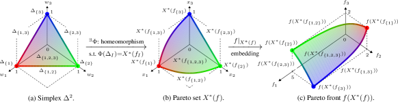
Figure 1: A simplicial problem $f=(f_{1},f_{2},f_{3})^{\top}:\mathbb{R}^{3}\to\mathbb{R}^{3}$. An $M$-objective problem $f$ is simplicial if the following conditions are satisfied: (i) there exists a homeomorphism $\Phi:\Delta^{M-1}\to X^{*}(f)$ such that $\Phi(\Delta_{I})=X^{*}(f_{I})$ for all $I\subseteq\{1,\dots,M\}$; (ii) the restriction $f|_{X^{*}(f)}:X^{*}(f)\to\mathbb{R}^{M}$ is a topological embedding (and thus so is $f\circ\Phi:\Delta^{M-1}\to\mathbb{R}^{M}$).

By using this advantage of the Bézier simplex model, we propose a novel strategy to construct a multi-objective optimization algorithm from a single-objective optimization. With a given single objective optimization algorithm, this scheme updates the Bézier simplex to obtain the Pareto set. In addition, we analyze the theoretical property of the multi-objective optimization algorithm derived from our scheme. Specifically, we first define Probably Approximately Correct (PAC) stability as an extension of the stability of optimization algorithms and prove that the PAC stability leads to an upper bound on the generalization gap in the sense of PAC learning. Our contributions are summarized as follows:

1. We devise a strategy to construct a multi-objective optimization algorithm from a single-objective optimization algorithm with the Bézier simplex. Unlike most of the existing multi-objective optimization methods, the algorithm derived from our scheme has the advantage of obtaining a parametric hyper-surface that represents the Pareto set of a given simplicial, Lipschitz continuous, differentiable multi-objective optimization problem to be solved.

2. We define PAC stability, which is an extension of the stability introduced by Hardt et al. [10] to the PAC learning settings and show that PAC stability gives an upper bound on the generalization gap with a high probability. Also, we prove that when we employ a gradient-based optimization algorithm as a single optimization algorithm, the derived multi-objective optimization algorithm is PAC stable.

3. We conducted numerical experiments and demonstrated that the multi-objective optimization algorithm constructed by our scheme achieved lower generalization errors than the existing multi-objective optimization algorithm. In addition, the algorithm given by our scheme can efficiently obtain the Pareto set with a small number of sample points.

Related Work

Kobayashi et al. [13] proposed Bèzier simplex fitting algorithms, the all-at-once fitting, and inductive skeleton fitting to describe Pareto fronts, and Tanaka et al. [22] analyzed the asymptotic risk of the fitting algorithms. The two fitting algorithms focus on post-optimization processes and assume that we have an approximate solution set of the Pareto set in advance. Thus, these algorithms by themselves cannot solve multi-objective optimization problems. Recently, Maree et al. [15] proposed a bi-objective optimization algorithm that updates the Bézier curve. However, this algorithm exploits the structure of the bi-objective optimization problem and can not be applied when the number of objective functions is more or equal to three. To the best of our knowledge, we are the first to propose a general framework of multi-objective optimization with the Bézier simplex and show its theoretical property.

2 Preliminaries

2.1 Probability simplex

Let $[M]=\{1,\dots,M\}$ be a set of $M$ points. We consider the set of probability distribution $\bm{t}$ over $[M]$. The set of probability distributions over $[M]$ is equal to the simplex

$$\Delta^{M-1}\coloneqq\left\{\mspace{2.0mu}{(t_{1},\dots,t_{M})^{\top}\in\mathbb{R}^{M}}\;\middle|\;{t_{m}\geq 0,\,\sum_{m=1}^{M}t_{m}=1}\mspace{2.0mu}\right\}.$$

Let $C(X)$ be the space of continuous functions over $X$, and we define the function $F\colon[M]\to C(X)$ by $F(m)=f_{m}$. Then, we have the expectation function

$$\begin{array}[]{rccc}\mathbb{E}(\bm{f})\colon&\Delta&\longrightarrow&C(X)\\ &\rotatebox{90.0}{$\in$}&&\rotatebox{90.0}{$\in$}\\ &\bm{t}&\longmapsto&\mathbb{E}_{\bm{t}}(F)\end{array}.$$

Furthermore, if $f_{m}$ is strongly convex for all $m\in[M]$, then the following function is well-defined:

$$\begin{array}[]{rccc}\arg\min\mathbb{E}(\bm{f})\colon&\Delta&\longrightarrow&X\\ &\rotatebox{90.0}{$\in$}&&\rotatebox{90.0}{$\in$}\\ &\bm{t}&\longmapsto&\arg\min\mathbb{E}_{\bm{t}}(F)\end{array}.$$

Note that $\mathbb{E}_{\bm{t}}(F)=\sum_{m}t_{m}f_{m}$ follows from the definition. $\mathbb{E}_{\bm{t}}(F)$ corresponds to the sum of a function chosen continuously along $\bm{t}$ from $\bm{f}$. As a direct consequence from Theorem 2 in Mizota et al. [18], the mapping $\arg\min\mathbb{E}(\bm{f})$ gives a continuous surjection onto $X^{\star}(\bm{f})$ if $f_{m}$ is strongly convex for all $m\in[M]$.

2.2 Simplicial Problem

A multi-objective optimization problem is characterized by its objective map $\bm{f}=(f_{1},\dots,f_{M})^{\top}\colon X\to\mathbb{R}^{M}$. We define the $J$-subsimplex for an index set $J\subseteq[M]$ by $\Delta^{M-1}_{J}\coloneqq\{(t_{1},\dots,t_{M})^{\top}\in\Delta^{M-1}\mid t_{m}=0\ (m\not\in J)\}$. The problem class we wish to consider is a problem in which the Pareto set/front has the simplex structure. Such problem class is defined as follows.

Definition 2.1 (Kobayashi et al. [13]).

A problem $\bm{f}\colon X\rightarrow\mathbb{R}^{M}$ is simplicial if there exists a map $\bm{\phi}\colon\Delta^{M-1}\rightarrow X$ such that for each non-empty subset $J\subseteq[M]$, its restriction $\bm{\phi}|_{\Delta^{(M-1)}_{J}}\colon\Delta^{M-1}_{J}\rightarrow X$ gives homeomorphisms

$$\bm{\phi}|_{\Delta^{M-1}_{J}}\colon\Delta^{M-1}_{J}\to X^{\star}(\bm{f}_{J}),\quad\bm{f}\circ\bm{\phi}|_{\Delta^{M-1}_{J}}\colon\Delta^{M-1}_{J}\to\bm{f}X^{\star}(\bm{f}_{J}).$$

We call such $\bm{\phi}$ and $\bm{f}\circ\bm{\phi}$ a triangulation of the Pareto set $X^{\star}(\bm{f})$ and the Pareto front $\bm{f}X^{\star}(\bm{f})$, respectively.

2.3 Bézier Simplex

Let $\mathbb{N}$ be the set of nonnegative integers and

$$\mathbb{N}^{M}_{D}\coloneqq\left\{\mspace{2.0mu}{(d_{1},\dots,d_{M})^{\top}\in\mathbb{N}^{M}}\;\middle|\;{\sum_{m=1}^{M}d_{m}=D}\mspace{2.0mu}\right\}.$$

For $\bm{t}\coloneqq(t_{1},\dots,t_{M})^{\top}\in\Delta^{M-1}$ and $\bm{d}\coloneqq(d_{1},\dots,d_{M})^{\top}\in\mathbb{N}^{M}_{D}$, we denote by $\bm{t}^{\bm{d}}$ a monomial $t_{1}^{d_{1}}\dots t_{M}^{d_{M}}$. The Bézier simplex of degree $D$ in $\mathbb{R}^{L}$ with control points $\{\bm{p}_{\bm{d}}\}_{\bm{d}\in\mathbb{N}^{M}_{D}}$ is defined as a map $\bm{b}\colon\Delta^{M-1}\to\mathbb{R}^{L}$:

$$\bm{b}(\bm{t}|\bm{P})\coloneqq\sum_{\bm{d}\in\mathbb{N}^{M}_{D}}\binom{D}{\bm{d}}\bm{t}^{\bm{d}}\bm{p}_{\bm{d}},$$ (1)

where $\binom{D}{\bm{d}}$ is a multinomial coefficient and $\bm{P}$ represents a matrix of vertically aligned control points:

$$\bm{P}\coloneqq\quantity(\bm{p}_{1},\dots,\bm{p}_{|\mathbb{N}^{M}_{D}|})^{\top}\in\mathbb{R}^{|\mathbb{N}^{M}_{D}|\times L}.$$

We define $\bm{z}(\bm{t})$ as

$$\bm{z}(\bm{t})\coloneqq\quantity[\binom{D}{\bm{d}_{1}}\bm{t}^{\bm{d}_{1}},\dots,\binom{D}{\bm{d}_{|\mathbb{N}^{M}_{D}|}}\bm{t}^{\bm{d}_{|\mathbb{N}^{M}_{D}|}}]^{\top}\in\mathbb{R}^{|\mathbb{N}^{M}_{D}|}.$$

Then, (1) can be represented as $\bm{b}(\bm{t}|\bm{P})=\bm{P}^{\top}\bm{z}(\bm{t})$. It is known that Bézier simplex is a universal approximator of continuous functions [13], and thus, the mapping $\arg\min\mathbb{E}(\bm{f})$ can be approximated by Bézier simplices in arbitrary precision. From this theoretical advantage, we construct a general framework to obtain a multi-objective optimization method $\mathcal{M}(A)$ from a single-objective optimization method $A$ with Bézier simplices.

3 Proposed Algorithm

\begin{overpic}[width=143.09538pt,trim=30.11249pt 30.11249pt 30.11249pt 30.11249pt,clip]{./figure/ma_step1} \put(85.0,30.0){\large$\longrightarrow$} \end{overpic}

(a) Generate solutions on the
Bézier simplex.

\begin{overpic}[width=143.09538pt,trim=30.11249pt 30.11249pt 30.11249pt 30.11249pt,clip]{./figure/ma_step2} \put(85.0,30.0){\large$\longrightarrow$} \end{overpic}

(b) Update each solution with $A_{\bm{t}^{(k)}_{n}}$.

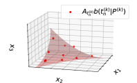
(c) Update the Bézier simplex.

Figure 2: Conceptual diagram of $\mathcal{M}(A)$ at the $k$th iteration; the red surfaces in (a) and (c) represent the Bèzier simplices.

Algorithm 1 Multi-objective Optimization Method $\mathcal{M}(A)$ of the Optimization Method $A$

1:  Set $k\leftarrow 1$ and the initial control point $\bm{P}^{(k)}$.

2:  while $k\leq K$ do

3:     Draw $\{\bm{t}^{(k)}_{n}\}_{n=1}^{N}$ for which each $\bm{t}^{(k)}_{n}$ is drawn i.i.d. from the uniform distribution on $\Delta^{M-1}$.

4:     Obtain $\{\bm{b}(\bm{t}^{(k)}_{n}|\bm{P}^{(k)})\}_{n=1}^{N}$ by (1).

5:     Obtain $\{A_{\bm{t}^{(k)}_{n}}(\bm{b}(\bm{t}^{(k)}_{n}|\bm{P}^{(k)}))\}_{n=1}^{N}$ from $A$.

6:     Update control points by (5).

7:     $k\leftarrow k+1$.

8:  end while

9:  return  $\bm{P}^{(K+1)}$.

A number of methods have been studied in the context of multi-objective optimization. Many of the methods are designed to apply to any multi-objective optimization problems; however, the individual methods are written in separate contexts and are not unified. Therefore, in this paper, we introduce a general framework to obtain a multi-objective optimization method $\mathcal{M}(A)$ from a single-objective optimization algorithm $A$. Moreover, in contrast to the existing methods finding a finite set that approximates Pareto set/front, we obtain a parametric hypersurface representing the Pareto set/front of multi-objective problems.

In our proposed algorithm, we obtain control points of a Bézier simplex that represents the Pareto set of a problem to be solved from a single-objective optimization algorithm $A$. In this paper, a single-objective optimization algorithm $A$ is a map from the direct product of the sample space and the space of loss functions $Z\times\mathcal{L}$ to the space of model parameters $\mathcal{W}$. Then, for any $\bm{t}\in\Delta^{M-1}$, we denote by $A_{\bm{t}}$ a single-objective optimization algorithm $A$ with the loss function $\mathbb{E}_{\bm{t}}(F)$, i.e., $A(-,\mathbb{E}_{\bm{t}}(F))$.

Our algorithm begins by setting the initial control points $\bm{P}^{(1)}$. At the $k$th iteration ($k\geq 1$), we randomly sample $\{\bm{t}^{(k)}_{n}\}^{N}_{n=1}$ from the uniform distribution on $\Delta^{M-1}$ and obtain data points $\{\bm{b}(\bm{t}^{(k)}_{n}|\bm{P}^{(k)})\}_{n=1}^{N}$ on the current Bézier simplex. Next, we update each $\bm{b}(\bm{t}^{(k)}_{n}|\bm{P}^{(k)})$ by $A_{\bm{t}^{(k)}_{n}}$, i.e.,

$$\bm{x}^{(k)}_{n}=A_{\bm{t}^{(k)}_{n}}\quantity(\bm{b}(\bm{t}^{(k)}_{n}|\bm{P}^{(k)})).$$ (2)

Then, we update the Bézier simplex with $\{(\bm{t}_{n}^{(k)},\bm{x}^{(k)}_{n})\}_{n=1}^{N}$. Specifically, we solve the following optimization problem to fit a Bézier simplex to $\{(\bm{t}_{n}^{(k)},\bm{x}^{(k)}_{n})\}_{n=1}^{N}$:

$$\underset{\bm{P}\in\mathbb{R}^{|\mathbb{N}^{M}_{D}|\times L}}{\mathrm{minimize}}\> \frac{1}{N}\sum_{n=1}^{N}\left\|\bm{x}^{(k)}_{n}-\bm{b}(\bm{t}^{(k)}_{n}|\bm{P})\right\|^{2}_{2},$$ (3)

where $\bm{P}$ is a variable to be optimized, and $\|\cdot\|_{2}$ denotes the Euclidean norm. Let $\bm{X}^{(k)}$ and $\bm{Z}^{(k)}$ be a matrix of vertically aligned $\bm{x}^{(k)}_{n}$ and $\bm{z}(\bm{t}^{(k)}_{n})$, respectively. Then, the problem (3) is reformulated as

$$\underset{\bm{P}\in\mathbb{R}^{|\mathbb{N}^{M}_{D}|\times L}}{\mathrm{minimize}}\>\frac{1}{N}\left\|\bm{X}^{(k)}-\bm{Z}^{(k)}\bm{P}\right\|^{2}_{F},$$ (4)

where $\|\cdot\|_{F}$ denotes the Frobenius norm. Since the optimization problem (4) is an unconstrained convex quadratic optimization, and it can be shown that $\bm{Z}^{(k)\top}\bm{Z}^{(k)}$ is regular with probability 1, the update rule for control points is described as

$$\bm{P}^{(k+1)}=\quantity(\bm{Z}^{(k)\top}\bm{Z}^{(k)})^{-1}\bm{Z}^{(k)\top}\bm{X}^{(k)}.$$ (5)

We repeat this procedure until $k$ reaches the maximum number of iterations specified by the user. We summarize the multi-objective optimization method in Algorithm 1 and show its conceptual diagram in Figure 2.

4 PAC Stability and Generalization Gap

Assume that there is an unknown distribution $\mathcal{D}$ over some space $Z$. We take $S=\left(\bm{t}_{1},\ldots,\bm{t}_{N}\right)$ of $N$ examples drawn i.i.d. from $\mathcal{D}$. Then the generalization error is defined by:

$$R[\bm{P}]\stackrel{{\scriptstyle\text{ def }}}{{=}}\mathbb{E}_{\bm{t}\sim\mathcal{D}}\ell(\bm{P};\bm{t}),$$

where $\ell$ is a loss function, and $\ell(\bm{P};\bm{t})$ denotes the loss of the model described by $\bm{P}$ with an input $\bm{t}$. Since the generalization error cannot be measured directly, we instead consider the empirical error defined by $R_{S}(\bm{P})\coloneqq\frac{1}{N}\sum^{N}_{n=1}\ell(\bm{P};\bm{t}_{n})$. Then, the generalization gap of $\bm{P}$ is defined as the difference between empirical error and generalization error, i.e.,

$$R_{S}(\bm{P})-R(\bm{P}).$$ (6)

We consider a potentially randomized algorithm $A$ (e.g., stochastic gradient descent) and the expectation value of (6):

$$\mathbb{E}_{A}\left[R_{S}[A(S)]-R[A(S)]\right].$$ (7)

To treat the approximate behavior of the expectation value with respect to the sample, we consider the following. First, take an event $C\subset Z^{N}$ that has a high probability of occurring. Then, the conditional generalization error under the condition $C$ is defined by:

$$\hat{R}[\bm{P}]\stackrel{{\scriptstyle\text{ def }}}{{=}}\mathbb{E}_{(\bm{t}_{1},...,\bm{t}_{N})\sim\mathcal{D}^{N}_{C}}\left[\frac{1}{N}\sum_{i=1}^{N}\ell(\bm{P};\bm{t}_{i})\right],$$

where $\mathcal{D}^{N}_{C}$ is the conditional probability distribution of $C$. Note that if $C=Z^{N}$, $\hat{R}[\bm{P}]$ is equal to $R[\bm{P}]$.

Next, we consider the approximate expectation value of (7) by

$$\hat{\mathbb{E}}_{S}\mathbb{E}_{A}\left[R_{S}[A(S)]-\hat{R}[A(S)]\right],$$ (8)

where $\hat{\mathbb{E}}_{S}$ is the conditional expectation value of $C$. This invariant allows us to discuss the expectation value of the generalization gap with respect to events.

The following introduces the definition of probably approximately correct (PAC) uniform stability. This is a PAC-like expansion of the uniform stability in [10].

Definition 4.1.

A randomized algorithm $A$ is PAC uniformly stable if for any $\varepsilon\in(0,1)$, there exists $\delta>0$ and an event $D_{\varepsilon}\subset Z^{N+1}$ which occurs with probability at least $1-\varepsilon$ such that

$$\sup_{\bm{t}}\mathbb{E}_{A}\left[\left|\ell(A(S);\bm{t})-\ell(A(S^{\prime});\bm{t})\right|\right]<\delta,$$ (9)

where $S=\left(\bm{t}_{1},\ldots,\bm{t}_{N}\right)$ and $S^{\prime}=\left(\bm{t}_{1},...,\bm{t}_{i}^{\prime},\ldots,\bm{t}_{N}\right)$ are samples differing in at most one example, drawn from $\mathcal{D}$, satisfying $\left(\bm{t}_{1},...,\bm{t}_{i},\bm{t}_{i}^{\prime},\bm{t}_{i+1}\ldots,\bm{t}_{N}\right)\in D_{\varepsilon}$. Furthermore, a PAC uniformly stable randomized algorithm $A$ is decomposable if for any $\varepsilon\in(0,1)$, there are events $B_{\varepsilon}\subset Z$ such that $D_{\varepsilon}=B_{\varepsilon}^{N+1}$.

With the PAC stability, we show the following that ensures that if an algorithm is PAC uniformly stable, the difference between its generalization and empirical error is small with high probability.

Theorem 4.2.

Let $A$ be a decomposable PAC uniformly stable randomized algorithm. Then, for any $\varepsilon\in(0,1)$ and $\delta>0$ in Definition 4.1, there exists an event $C_{\varepsilon}\subset Z^{N}$ which occurs with probability at least $1-\varepsilon$ such that,

$$\left|\hat{\mathbb{E}}_{S}\mathbb{E}_{A}\left[R_{S}[A(S)]-\hat{R}[A(S)]\right]\right|<\delta,$$

where $\hat{\mathbb{E}}_{S}$ is the conditional expectation value of $C_{\varepsilon}$ and $\hat{R}$ is the conditional generalization error under the condition $C_{\varepsilon}$.

The proof of Theorem 4.2 is shown in Appendix.

5 A surface-wise gradient descent method

Next, we discuss the case that $A$ is a gradient descent method. In this case, the update rule (2) can be represented as

$$\bm{x}^{(k)}_{n} =\bm{b}(\bm{t}^{(k)}_{n}|\bm{P})-\alpha^{(k)}\mathrm{d}_{\bm{x}}f\quantity(\bm{b}(\bm{t}^{(k)}_{n}|\bm{P})\left|\,\bm{t}^{(k)}_{n}\right.)=\bm{b}(\bm{t}^{(k)}_{n}|\bm{P})-\alpha^{(k)}J_{\bm{f}}\quantity(\bm{b}(\bm{t}^{(k)}_{n}|\bm{P}))^{\top}\bm{t}^{(k)}_{n},$$ (10)

where $\alpha^{(k)}\in(0,1]$ is a step size at the $k$th iteration, $\mathrm{d}_{\bm{x}}$ is a first derivative with respect to $\bm{x}$, $f(\cdot|\bm{t})$ is a weighted sum of objective functions $f_{1},\dots,f_{M}$ by $\bm{t}$, and $J_{\bm{f}}(\bm{x})$ is a matrix of vertically aligned gradient of $f_{m}$ at $\bm{x}$ defined by $J_{\bm{f}}(\bm{x})\coloneqq\quantity(\nabla f_{1}(\bm{x}),\dots,\nabla f_{M}(\bm{x}))^{\top}\in\mathbb{R}^{M\times L}$. Let us define $\bm{B}^{(k)}$ and $\bm{G}^{(k)}$ as

$$\bm{B}^{(k)}\coloneqq\bm{Z}^{(k)}\bm{P}^{(k)},\;\bm{G}^{(k)}\coloneqq\matrixquantity[(\bm{t}^{(k)}_{1})^{\top}J_{\bm{f}}(\bm{P}^{(k)\top}\bm{z}_{1})\\ \vdots\\ (\bm{t}^{(k)}_{N})^{\top}J_{\bm{f}}(\bm{P}^{(k)\top}\bm{z}_{N})]$$

Then, the update rule (10) is rewritten as

$$\bm{X}^{(k)}=\bm{B}^{(k)}-\alpha^{(k)}\bm{G}^{(k)}.$$

With this notation, the update rule for the control points (5) is represented as

$$\bm{P}^{(k+1)}=\bm{P}^{(k)}-\alpha^{(k)}\quantity(\bm{Z}^{(k)\top}\bm{Z}^{(k)})^{-1}\bm{Z}^{(k)\top}\bm{G}^{(k)}.$$ (11)

We describe the surface-wise gradient descent method in Algorithm 2.

Algorithm 2 Surface-wise Gradient Descent Method

1:  Set $k\leftarrow 1$ and the initial control point $\bm{P}^{(k)}$.

2:  while $k\leq K$ do

3:     Draw $\{\bm{t}^{(k)}_{n}\}_{n=1}^{N}$ for which each $\bm{t}^{(k)}_{n}$ is drawn i.i.d. from the uniform distribution on $\Delta^{M-1}$.

4:     Obtain $\{\bm{b}(\bm{t}^{(k)}_{n}|\bm{P}^{(k)})\}_{n=1}^{N}$ by (1).

5:     Update $\{\bm{b}(\bm{t}^{(k)}_{n}|\bm{P}^{(k)})\}_{n=1}^{N}$ by (10).

6:     Update control points by (11).

7:     $k\leftarrow k+1$.

8:  end while

9:  return  $\bm{P}^{(K+1)}$.

6 PAC Stability of the surface-wise gradient descent method

We prove that the surface-wise gradient descent is PAC uniformly stable. All omitted proofs are shown in Appendix. Hereinafter, we make the following mild assumption about the objective function.

Assumption 6.1.

All the objective functions $f_{1},\dots,f_{M}$ are $\mu$-Lipschitz continuous and differentiable on $X$.

Let $\bm{x}^{\star}\colon\Delta^{M-1}\to X^{\star}(\bm{f})$ be a map from $\Delta^{M-1}$ to the Pareto set of $\bm{f}$. For $\bm{P}$, we define a loss function as

$$\ell(\bm{P};\bm{t})\coloneqq\|\bm{b}(\bm{t}|\bm{P})-\bm{x}^{\star}(\bm{t})\|_{2}.$$ (12)

Since $X^{*}(\bm{f})$ is unknown, we can not take a sample directly from $X^{\star}(\bm{f})$. Instead, we take a sample $\bm{t}=\{\bm{t}_{n}\}^{N}_{n=1}$ drawn i.i.d. from the uniform distribution over $\Delta^{M-1}$.

To prove that Algorithm 2 is PAC uniformly stable, we first show two propositions in advance. Note that the following two propositions can respectively be regarded as an extension of the concept of boundedness and expansiveness introduced in [10] to analyze the stability of an optimization algorithm.

Lemma 6.2.

Let $U>0$ be a constant satisfying $\max_{\bm{t}\in\Delta^{M-1}}\|\bm{z}(\bm{t})\|_{2}\leq U$. Let $\varphi_{\bm{T}}$ be the update rule with parameter $\bm{T}=\{\bm{t}_{n}\}^{N}_{n=1}$ in (11). Then there exists some $\eta>0$, and we have the following inequality with probability at least $1-\varepsilon$:

$$\left\|\varphi_{\bm{T}}(\bm{P})-\bm{P}\right\|_{F}\leq\eta NU\mu.$$

Lemma 6.3.

Let $\eta>0$ and $U>0$ be constants as in Lemma 6.2. For $\bm{T}=\{\bm{t}_{n}\}^{N}_{n=1}$ and $\bm{T}^{\prime}=\{\bm{t}^{\prime}_{n}\}^{N}_{n=1}$ such that the difference between $\bm{T}$ and $\bm{T}^{\prime}$ lies only in one example, there exists some $\zeta>0$, and we have the following with probability at least $1-\varepsilon$:

$$\left\|\varphi_{\bm{T}}(\bm{P})-\varphi_{\bm{T}^{\prime}}(\bm{P})\right\|_{F}\leq\mu U\quantity(\eta+\zeta N).$$

Let $\{\bm{T}_{i}\}^{K}_{i=1}$ and $\{\bm{T}^{\prime}_{i}\}^{K}_{i=1}$ be parameters whose difference lies only in the $k$th element, and $\bm{P}^{(K+1)}$ and $\bm{P}^{\prime(K+1)}$ be respectively the output of Algorithm 2 with $\{\bm{T}_{i}\}^{K}_{i=1}$ and $\{\bm{T}^{\prime}_{i}\}^{K}_{i=1}$. From Lemmas 6.2, LABEL: and 6.3, we show that $\|\bm{P}^{(K+1)}-\bm{P}^{\prime(K+1)}\|_{F}$ is bounded above with arbitrary probability.

Lemma 6.4.

Let $U>0,\,\eta>0$ and $\zeta>0$ be constants as in Lemma 6.3. Suppose that we run Algorithm 2 for $K$ iterations with parameters $\{\bm{T}_{i}\}^{K}_{i=1}$ and $\{\bm{T}^{\prime}_{i}\}^{K}_{i=1}$ whose difference lies only in the $k$th element. Then, we have the following with probability at least $1-\varepsilon$:

$$\left\|\bm{P}^{(K+1)}-\bm{P}^{\prime(K+1)}\right\|_{F}\leq 2\mu\eta U\quantity{1+\quantity(K-k+\frac{\zeta}{\eta})N}.$$

Now, we are ready to show that Algorithm 2 is PAC uniformly stable.

Theorem 6.5.

Assume that $\alpha^{(k)}\in(0,1]$ for all $k\in[K]$. Then, Algorithm 2 is PAC uniformly stable.

From Theorems 4.2 and 6.5, we obtain an upper bound of the generalization gap of Algorithm 2 if Algorithm 2 is decomposable.

7 Numerical Experiments

To verify that the Pareto set can be accurately approximated by a Bézier simplex obtained by our proposed method (Algorithm 2), we applied the proposed method to three multi-objective problems, which are known to be simplicial. Notice that the formulation of skew-$M$MMD includes some important problems, such as the group Lasso in sparse modeling [28]. The definition of each problem instance is shown in Appendix E. In Algorithm 2, we set the degree of Bézier simplex as $D=3$, the initial control points as $\bm{P}^{(1)}=\bm{O}$, which is the zero matrix. Also, we set $K=1000$ and $\alpha^{(k)}=\frac{1}{k}$. The number of points to be sampled from a simplex in each iteration was tested for $N\in\{30,50,100\}$.

As a baseline, we used NSGA-II with the Bézier simplex fitting [13]. Specifically, we obtain approximated Pareto solution samples by NSGA-II [5] implemented in jMetal [1], which is provided under MIT license, with default parameters except for population size. Then, we fit a Bézier simplex of degree $D=3$ to the approximated Pareto solutions by the all-at-once method proposed in Kobayashi et al. [13]. We set the number of population size as $p\in\{30,50,100\}$. We implemented these algorithms in Python 3.8.10, and the experiments were performed on a Windows 10 PC with an Intel(R) Xeon(R) W-1270 CPU $3.40\text{\,}\mathrm{G}\mathrm{H}\mathrm{z}$ and $64\text{\,}\mathrm{G}\mathrm{B}$ RAM.

7.1 MSEs comparison

First, we picked up a simplicial problem instance whose $\bm{x}^{\star}$ is analytically obtained and evaluated how accurate an obtained Bézier simplex approximates the Pareto set. In this experiment, we used scaled-MED, which is the three-objective problem with three variables and is known to be simplicial. The problem definition is shown in Appendix E. To evaluate the approximation accuracy of the estimated Bézier simplex, we used the mean squared error (MSE) defined by $\mathrm{MSE}\coloneqq\frac{1}{N}\sum^{N}_{n=1}\|\bm{b}(\hat{\bm{t}}_{n}|\bm{P})-\bm{x}^{\star}(\hat{\bm{t}}_{n})\|^{2}_{2}$, where $\bm{x}^{\star}$ is a map from a weight to the minimizer of the corresponding scalarizing function. The map $\bm{x}^{\star}$ for scaled-MED is shown in Appendix F. To calculate MSE, we randomly sample $\{\hat{\bm{t}}_{n}\}^{10000}_{n=1}$ i.i.d. from the uniform distribution on $\Delta^{2}$. We repeated the experiments 20 times with different parameters and computed the average and the standard deviations of MSEs.

Table 1 shows the average and the standard deviation of the MSEs with $N\in\{30,50,100\}$ for Algorithm 2 and $p\in\{30,50,100\}$ for NSGA-II. In Table 1, we highlighted the best score of MSE out of the proposed and baseline method where the difference is significant with the significance level $\mathrm{p}=0.01$ by the Wilcoxon rank-sum test. Table 1 shows that the Bézier simplex obtained by our proposed method can represent Pareto set well. Also, the MSEs of our method decrease with larger $N$. This result supports the PAC uniform stability of Algorithm 2. Figure 4 shows the Bézier simplex obtained by our proposed method, and Figure 4 shows the Bézier simplex obtained by the all-at-once with NSGA-II. The true Pareto set of scaled-MED for our setting is known to be a curved triangle that can be triangulated into three vertices. In Figure 4, the Bézier simplex obtained by our method approximates the Pareto set well even with $N=30$.

Table 1: MSE (avg.$\pm$s.d. over 20 trials) for scaled-MED.

Problem	Proposed		NSGA-II + all-at-once
scaled-MED	$N=30$	5.51e-05$\pm$2.40e-06	$p=30$	1.51e-01$\pm$1.56e-03
	$N=50$	4.43e-05$\pm$1.88e-06	$p=50$	8.23e-02$\pm$6.80e-04
	$N=100$	3.78e-05$\pm$1.30e-06	$p=100$	1.25e-01$\pm$1.32e-03

Table 2: GD and IGD (avg.$\pm$s.d. over 20 trials) for skew-3MED and skew-3MMD.

Problem		Proposed		NSGA-II + all-at-once
skew-3MED	GD	$N=30$	6.22e-02$\pm$1.46e-03	$p=30$	1.76e-01$\pm$3.67e-03
		$N=50$	5.50e-02$\pm$4.57e-04	$p=50$	1.22e-01$\pm$2.00e-03
		$N=100$	5.38e-02$\pm$7.90e-04	$p=100$	6.33e-02$\pm$7.90e-04
	IGD	$N=30$	9.50e-02$\pm$3.68e-04	$p=30$	1.38e-01$\pm$8.63e-04
		$N=50$	8.84e-02$\pm$3.29e-04	$p=50$	1.33e-01$\pm$8.92e-04
		$N=100$	8.45e-02$\pm$3.42e-04	$p=100$	8.86e-02$\pm$6.02e-04
skew-3MMD	GD	$N=30$	5.45e-02$\pm$1.32e-03	$p=30$	2.04e-01$\pm$6.07e-03
		$N=50$	5.16e-02$\pm$9.85e-04	$p=50$	9.34e-01$\pm$2.15e-03
		$N=100$	5.06e-02$\pm$1.07e-03	$p=100$	6.60e-02$\pm$1.07e-03
	IGD	$N=30$	6.40e-02$\pm$4.69e-04	$p=30$	1.00e-01$\pm$1.45e-03
		$N=50$	6.38e-02$\pm$4.27e-04	$p=50$	7.64e-02$\pm$9.55e-04
		$N=100$	6.54e-02$\pm$4.81e-04	$p=100$	7.23e-02$\pm$8.46e-04

7.2 GDs and IGDs comparison

Next, we validate the practicality of the proposed method in more practical settings. In this experiment, we used two simplicial problem instances: skew-$3$MED and skew-$3$MMD, whose $\bm{x}^{\star}$ cannot be represented in a closed-form. We show their definitions in Appendix E. We used the generational distance (GD) [23] and the inverted generational distance (IGD) [30] to evaluate how accurately the estimated Bézier simplex approximates the Pareto set. GD and IGD are defined by:

$$\mathrm{GD}(X,Y)\coloneqq\frac{1}{|X|}\sum_{\bm{x}\in X}\min_{\bm{y}\in Y}\|\bm{x}-\bm{y}\|_{2},\quad\mathrm{IGD}(X,Y)\coloneqq\frac{1}{|Y|}\sum_{\bm{y}\in Y}\min_{\bm{x}\in X}\|\bm{x}-\bm{y}\|_{2},$$

where $X$ is a finite set whose elements are sampled from an estimated hyper-surface and $Y$ is a validation set. We can say that the obtained Bézier simplex is close to the Pareto set if and only if both GD and IGD are small. As a validation set $Y$, we generated approximate Pareto solutions by NSGA-II with the population size of $1000$. To construct $X$, we randomly sample $\{\hat{\bm{t}}_{n}\}^{1000}_{n=1}$ i.i.d. from the uniform distribution on $\Delta^{2}$ and obtain sample points on the estimated Bézier simplex. We repeated the experiments 20 times with different parameters and computed the average and the standard deviations of their GDs and IGDs.

Table 2 shows the average and the standard deviation of the GDs and IGDs when $N\in\{30,50,100\}$ and $p\in\{30,50,100\}$. In Table 2, we highlighted the best score of GD and IGD where the difference is at a significant with significance level $\mathrm{p}=0.01$ by the Wilcoxon rank-sum test. Table 2 shows that the proposed method achieved better GD and IGD for skew-3MED and skew-3MMD. The differences are pronounced in the results of small sample/population size, which implies our method obtains a Bézier simplex approximating Pareto set well.

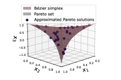
(a) $N=30$

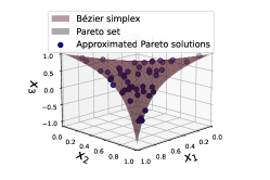
(b) $N=50$

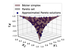
(c) $N=100$

Figure 3: Results for Algorithm 2 with the sample size of $30,50$, and $100$.

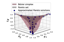
(a) $p=30$

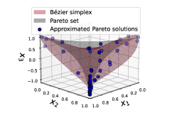
(b) $p=50$

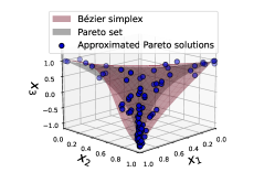
(c) $p=100$

Figure 4: Results for NSGA-II and the all-at-once with the population size of $30,50$, and $100$.

8 Conclusion

In this paper, we have devised a general strategy to construct a multi-objective optimization algorithm from a single objective method with the Bézier simplex. Also, we have defined the PAC stability of optimization algorithms and proved that this stability gives us an upper bound on the generalization gap in the sense of PAC learning. Our theoretical analysis showed that if we construct a multi-objective optimization algorithm from a gradient-based single-objective optimization algorithm, the resultant algorithm is PAC stable. In our numerical experiments, we have demonstrated the multi-objective optimization algorithm on the basis of our scheme gives better generalization gaps and approximation accuracies of the Pareto set than the existing algorithm for simplicial problems. As a concluding remark, we have to note that this study is limited to treat simplicial problems. It would be interesting for future studies to extend this study to non-simplicial cases.

Appendix A Proof of Theorem 4.2

Proof.

We denote two independent random samples by $S=\left(\bm{t}_{1},\ldots,\bm{t}_{N}\right)$, $S^{\prime}=\left(\bm{t}_{1}^{\prime},\ldots,\bm{t}_{N}^{\prime}\right)$. Let $S^{(i)}=\left(\bm{t}_{1},\ldots,\bm{t}_{i-1},\bm{t}_{i}^{\prime},\bm{t}_{i+1},\dots,\bm{t}_{N}\right)$ be the sample that is same as $S$ except in the $i$th example where we replace $t_{i}$ with $t_{i}^{\prime}$. Since $D_{\varepsilon}=B_{\varepsilon}^{N+1}$, $\left(\bm{t}_{1},\ldots,\bm{t}_{i},\bm{t}_{i}^{\prime},\bm{t}_{i+1},\dots,\bm{t}_{N}\right)\in D_{\varepsilon}$ for any $i$ if and only if $S,S^{\prime}\in C_{\varepsilon}:=B_{\varepsilon}^{N}$. In this case, we have

$$\mathbb{E}_{A}\left[\left|\ell(A(S);\bm{t}_{i})-\ell(A(S^{(i)});\bm{t}_{i})\right|\right]<\delta.$$

Then adding the inequalities for $i$ and applying the triangle inequality, we obtain

$$\left|\mathbb{E}_{A}\left[\frac{1}{N}\sum_{i=1}^{N}\ell(A(S);\bm{t}_{i})-\frac{1}{N}\sum_{i=1}^{N}\ell(A(S^{(i)});\bm{t}_{i})\right]\right|<\delta.$$

Let us denote the conditional probability distribution of $\mathcal{D},\mathcal{D}^{N}$ under the condition $B_{\varepsilon},C_{\varepsilon}$ by $\mathcal{B}_{\varepsilon},\mathcal{C}_{\varepsilon}$ respectively. Then we have

$$\left|\mathbb{E}_{(S,S^{\prime})\sim\mathcal{C}_{\varepsilon}^{2}}\mathbb{E}_{A}\left[\frac{1}{N}\sum_{i=1}^{N}\ell(A(S);\bm{t}_{i})-\frac{1}{N}\sum_{i=1}^{N}\ell(A(S^{(i)});\bm{t}_{i})\right]\right|<\delta.$$

Here, we have

$$\mathbb{E}_{(S,S^{\prime})\sim\mathcal{C}_{\varepsilon}^{2}}\mathbb{E}_{A}\left[\frac{1}{N}\sum_{i=1}^{N}\ell\left(A(S);\bm{t}_{i}\right)\right]=\mathbb{E}_{S\sim\mathcal{C}_{\varepsilon}}\mathbb{E}_{A}\left[\frac{1}{N}\sum_{i=1}^{N}\ell\left(A(S);\bm{t}_{i}\right)\right]=\hat{\mathbb{E}}_{S}\mathbb{E}_{A}\left[R_{S}[A(S)]\right],$$

and

$$\mathbb{E}_{(S,S^{\prime})\sim\mathcal{C}_{\varepsilon}^{2}}\mathbb{E}_{A}\left[\frac{1}{N}\sum_{i=1}^{N}\ell\left(A(S^{(i)});\bm{t}_{i}\right)\right] =\mathbb{E}_{(S,S^{\prime})\sim\mathcal{C}_{\varepsilon}^{2}}\mathbb{E}_{A}\left[\frac{1}{N}\sum_{i=1}^{N}\ell\left(A(S);\bm{t}^{\prime}_{i}\right)\right]$$

$$=\mathbb{E}_{S\sim\mathcal{C}_{\varepsilon}}\mathbb{E}_{A}\mathbb{E}_{S^{\prime}\sim\mathcal{C}_{\varepsilon}}\left[\frac{1}{N}\sum_{i=1}^{N}\ell\left(A(S);\bm{t}^{\prime}_{i}\right)\right]$$

$$=\hat{\mathbb{E}}_{S}\mathbb{E}_{A}\left[\hat{R}[A(S)]\right],$$

where $\hat{\mathbb{E}}_{S}$ is the conditional expectation value of $C_{\varepsilon}$ and $\hat{R}[A(S)]$ is the conditional generalization error of $C_{\varepsilon}$. Thus we obtain the inequality in the theorem.

Finally, we have

$$\mathbb{P}\quantity(C_{\varepsilon})=\mathbb{P}\quantity(B_{\varepsilon})^{N}=\mathbb{P}\quantity(D_{\varepsilon})^{\frac{N}{N+1}}>\mathbb{P}\quantity(D_{\varepsilon})>1-\varepsilon,$$

which completes the proof. ∎

Appendix B Proofs of Lemmas 6.2 and 6.3

We first show the three lemmas in advance.

Lemma B.1.

For all $\varepsilon\in(0,1)$, there exists $\eta>0$ satisfying

$$\mathbb{P}\quantity(\min_{i}\lambda_{\min}\quantity(\bm{Z}(\bm{T}_{i})^{\top}\bm{Z}(\bm{T}_{i}))>\eta)\geq 1-\varepsilon,$$

where $\lambda_{\min}(\bm{A})$ denotes the minimal eigenvalue of $\bm{A}$ and $\bm{T}_{i}=\{\bm{t}^{(i)}_{n}\}^{N}_{n=1}$ is drawn i.i.d. from the uniform distribution on $\Delta^{M-1}$ for $i\in[K+1]$.

Proof.

Consider the set

$$A_{0}\coloneqq\left\{\mspace{2.0mu}{\{\bm{T_{i}}\}_{i=1}^{K+1}\subseteq(\Delta^{M-1})^{K+1}}\;\middle|\;{\min_{i}\lambda_{\min}\quantity(\bm{Z}(\bm{T_{i}})^{\top}\bm{Z}(\bm{T_{i}}))=0}\mspace{2.0mu}\right\}.$$

Since $\bm{Z}(\bm{T}_{i})^{\top}\bm{Z}(\bm{T}_{i})$ is a symmetric matrix, it has non-negative eigenvalues and $\bm{Z}(\bm{T}_{i})^{\top}\bm{Z}(\bm{T}_{i})$ has zero eigenvalue if and only if the determinant of $\bm{Z}(\bm{T}_{i})^{\top}\bm{Z}(\bm{T}_{i})$ is zero. Hence, $A_{0}$ is a subset of

$$\left\{\mspace{2.0mu}{\{\bm{t}_{n}\}_{n=1}^{N}\subseteq\Delta^{M-1}}\;\middle|\;{\prod_{i}\det(\bm{Z}(\bm{T}_{i})^{\top}\bm{Z}(\bm{T}_{i}))=0}\mspace{2.0mu}\right\}.$$

Therefore, $A_{0}$ is equal to the zero set of a polynomial. This implies $\mathbb{P}(A_{0})=0$. Considering the set

$$A_{\eta}\coloneqq\left\{\mspace{2.0mu}{\{\bm{T}_{i}\}_{i=1}^{K+1}\subseteq(\Delta^{M-1})^{K+1}}\;\middle|\;{\min_{i}\lambda_{\min}\quantity(\bm{Z}(\bm{T_{i}})^{\top}\bm{Z}(\bm{T_{i}}))\leq\eta}\mspace{2.0mu}\right\},$$

then we have

$$\mathbb{P}(A_{\eta})\to\mathbb{P}(A_{0})=0\quad(\eta\to 0).$$

This implies that for all $\varepsilon\in(0,1)$ there exists some $\eta>0$ such that

$$\Pr(\left\{\mspace{2.0mu}{\{\bm{T}_{i}\}_{i=1}^{K+1}\subseteq(\Delta^{M-1})^{K+1}}\;\middle|\;{\min_{i}\lambda_{\min}\quantity(\bm{Z}(\bm{T}_{i})^{\top}\bm{Z}(\bm{T}_{i}))\leq\eta}\mspace{2.0mu}\right\})<\varepsilon.$$ (13)

The proof is completed by taking the complementary event. ∎

Lemma B.2.

For all $\varepsilon\in(0,1)$, there exists $\zeta>0$ satisfying

$$\mathbb{P}\quantity(\max_{i}\left\|\bm{Z}(\bm{T}_{i})^{\top}\bm{Z}(\bm{T}_{i})\right\|_{F}<\zeta)\geq 1-\varepsilon,$$ (14)

where $\bm{T}_{i}=\{\bm{t}^{(i)}_{n}\}_{n=1}^{N}$ is drawn i.i.d. from the uniform distribution on $\Delta^{M-1}$ for $i\in[K+1]$.

Proof.

Since $\bm{Z}(\bm{T}_{i})^{\top}\bm{Z}(\bm{T}_{i})$ is a symmetric matrix, there exists an orthogonal matrix $\bm{Q}_{i}$ such that $\bm{Z}(\bm{T}_{i})^{\top}\bm{Z}(\bm{T}_{i})=\bm{Q}_{i}\bm{\Lambda}_{i}\bm{Q}_{i}^{\top}$ where $\bm{\Lambda}_{i}$ is a diagonal matrix whose diagonal entry is the eigenvalue of $\bm{Z}(\bm{T}_{i})^{\top}\bm{Z}(\bm{T}_{i})$. According to Lemma B.1, $\bm{Z}(\bm{T}_{i})^{\top}\bm{Z}(\bm{T}_{i})$ is a regular matrix with probability at least $1-\varepsilon$ for all $i\in[K+1]$. Hence, we have the following with probability at least $1-\varepsilon$:

$$\max_{i}\left\|\quantity(\bm{Z}(\bm{T}_{i})^{\top}\bm{Z}(\bm{T}_{i}))^{-1}\right\|_{F} =\max_{i}\|\bm{Q}_{i}^{\top}\bm{\Lambda}_{i}^{-1}\bm{Q}_{i}\|_{F}$$

$$=\max_{i}\|\bm{\Lambda}_{i}^{-1}\|_{F}$$

$$=\max_{i}\sqrt{\sum_{n=1}^{|\mathbb{N}^{M}_{D}|}\frac{1}{\lambda^{2}_{n}(\bm{Z}(\bm{T}_{i})^{\top}\bm{Z}(\bm{T}_{i}))}}$$

$$\leq\sqrt{\frac{|\mathbb{N}^{M}_{D}|}{\min_{i}\lambda^{2}_{\min}(\bm{Z}(\bm{T}_{i})^{\top}\bm{Z}(\bm{T}_{i}))}}$$

$$<\frac{\sqrt{|\mathbb{N}^{M}_{D}|}}{\eta},$$

where the second equality follows from the fact that the Frobenius norm is unitarily invariant, and the second inequality follows from Lemma B.1. The proof is completed by letting $\zeta$ be some real number greater than or equal to $\frac{\sqrt{|\mathbb{N}^{M}_{D}|}}{\eta}$. ∎

Lemma B.3.

Let $U>0$ be a constant satisfying $\max_{\bm{t}\in\Delta^{M-1}}\|\bm{z}(\bm{t})\|_{2}\leq U$. Then, for any $\bm{T}\subseteq\Delta^{M-1}$, we have

$$\left\|\bm{Z}(\bm{T})^{\top}\bm{G}(\bm{T})\right\|_{F}\leq NU\mu.$$ (15)

Proof.

First, we show that $\|\bm{z}(\bm{t})\|_{2}$ is bounded above for any $\bm{t}\in\Delta^{M-1}$. Since $\bm{z}$ is a continuous function over $\bm{t}$ whose domain $\Delta^{M-1}$ is compact, there exists upper bound $U>0$ for any $\bm{t}\in\Delta^{M-1}$. Next, we show that $\|\bm{Z}(\bm{T})^{\top}\bm{G}(\bm{T})\|_{F}$ is bounded above. For any $\bm{T}\coloneqq\quantity{\bm{t}_{n}}^{N}_{n=1}\subseteq\Delta^{M-1}$, we have

$$\bm{Z}(\bm{T})^{\top}\bm{G}(\bm{T})=(\bm{z}_{1},\dots,\bm{z}_{N})\begin{bmatrix}\bm{t}_{1}^{\top}J_{\bm{f}}(\bm{P}^{\top}\bm{z}_{1})\\ \vdots\\ \bm{t}_{N}^{\top}J_{\bm{f}}(\bm{P}^{\top}\bm{z}_{N})\\ \end{bmatrix}=\sum_{n=1}^{N}\bm{z}_{n}\bm{t}_{n}^{\top}J_{\bm{f}}(\bm{P}^{\top}\bm{z}_{n}).$$

Therefore,

$$\left\|\bm{Z}(\bm{T})^{\top}\bm{G}(\bm{T})\right\|_{F} =\left\|\sum_{n=1}^{N}\bm{z}_{n}\bm{t}_{n}^{\top}J_{\bm{f}}(\bm{P}^{\top}\bm{z}_{n})\right\|_{F}$$

$$\leq\sum_{n=1}^{N}\left\|\bm{z}_{n}\bm{t}_{n}^{\top}J_{\bm{f}}(\bm{P}^{\top}\bm{z}_{n})\right\|_{F}$$

$$\leq\sum_{n=1}^{N}\left\|\bm{z}_{n}\right\|_{2}\left\|\bm{t}_{n}^{\top}J_{\bm{f}}(\bm{P}^{\top}\bm{z}_{n})\right\|_{2}$$

$$=\sum_{n=1}^{N}\left\|\bm{z}_{n}\right\|_{2}\left\|\sum_{m=1}^{M}t_{nm}\nabla f_{m}(\bm{P}^{\top}\bm{z})\right\|_{2}$$

$$\leq\sum_{n=1}^{N}U\mu=NU\mu.$$

The last inequality holds by the fact that the term $\sum_{m=1}^{M}t_{nm}\nabla f_{m}(\bm{P}^{\top}\bm{z})$ is a convex combination of $\nabla f_{1}(\bm{P}^{\top}\bm{z}),\dots,\nabla f_{M}(\bm{P}^{\top}\bm{z})$ and the assumption that every function $f_{1},\dots,f_{M}$ is $\mu$-Lipschitz continuous. ∎

Finally, we show Lemmas 6.2 and 6.3.

Proof of Lemma 6.2.

By (11), we have

$$\left\|\varphi_{\bm{T}}(\bm{P})-\bm{P}\right\|_{F} =\alpha^{(k)}\left\|\quantity(\bm{Z}^{\top}\bm{Z})^{-1}\bm{Z}^{\top}\bm{G}\right\|_{F}$$

$$\leq\left\|\quantity(\bm{Z}^{\top}\bm{Z})^{-1}\right\|_{F}\left\|\bm{Z}^{\top}\bm{G}\right\|_{F}.$$

Let $\eta>0$ be a constant as in Lemma B.2. From Lemmas B.2 and B.3, we have the following with probability at least $1-\varepsilon$:

$$\left\|\varphi_{\bm{t}}(\bm{P})-\bm{P}\right\|_{F}\leq\eta NU\mu.$$

∎

Proof of Lemma 6.3.

Let $\bm{T}$, $\bm{T}^{\prime}$ and $\tilde{\bm{T}}$ be

$$\bm{T} =\quantity{\bm{t}_{1},\dots,\bm{t}_{N-1},\bm{t}_{N}},$$

$$\bm{T}^{\prime} =\quantity{\bm{t}_{1},\dots,\bm{t}_{N-1},\bm{t}^{\prime}_{N}},$$

$$\tilde{\bm{T}} =\quantity{\bm{t}_{1},\dots,\bm{t}_{N-1},\bm{t}_{N},\bm{t}^{\prime}_{N}}.$$

Let $\tilde{\bm{Z}}$ be a matrix constructed by $\tilde{\bm{T}}$. By Sherman-Morrison formula, we have

$$(\tilde{\bm{Z}}^{\top}\tilde{\bm{Z}})^{-1} =(\bm{Z}^{\top}\bm{Z}+\bm{z}_{N+1}\bm{z}_{N+1}^{\top})^{-1}$$

$$=(\bm{Z}^{\top}\bm{Z})^{-1}+\frac{(\bm{Z}^{\top}\bm{Z})^{-1}\bm{z}_{N+1}\bm{z}_{N+1}^{\top}(\bm{Z}^{\top}\bm{Z})^{-1}}{1+\bm{z}_{N+1}^{\top}(\bm{Z}^{\top}\bm{Z})^{-1}\bm{z}_{N+1}}.$$

Let $\varphi_{\bm{T}}(\bm{P})$ be the control points obtained by Algorithm 2 with $\bm{T}$. Then, we have

$$\varphi_{\tilde{\bm{T}}}(\bm{P})-\varphi_{\bm{T}}(\bm{P}) =(\tilde{\bm{Z}}^{\top}\tilde{\bm{Z}})^{-1}\tilde{\bm{Z}}^{\top}\tilde{\bm{G}}-(\bm{Z}^{\top}\bm{Z})^{-1}\bm{Z}^{\top}\bm{G}$$

$$=(\bm{Z}^{\top}\bm{Z})^{-1}(\tilde{\bm{Z}}^{\top}\tilde{\bm{G}}-\bm{Z}^{\top}\bm{G})+\frac{(\bm{Z}^{\top}\bm{Z})^{-1}\bm{z}_{N+1}\bm{z}_{N+1}^{\top}(\bm{Z}^{\top}\bm{Z})^{-1}\tilde{\bm{Z}}^{\top}\tilde{\bm{G}}}{1+\bm{z}_{N+1}^{\top}(\bm{Z}^{\top}\bm{Z})^{-1}\bm{z}_{N+1}}$$

$$=(\bm{Z}^{\top}\bm{Z})^{-1}(\bm{z}_{N+1}\bm{t}_{N+1}^{\top}J_{\bm{f}}(\bm{P}^{\top}\bm{z}_{N+1}))+\frac{(\bm{Z}^{\top}\bm{Z})^{-1}\bm{z}_{N+1}\bm{z}_{N+1}^{\top}(\bm{Z}^{\top}\bm{Z})^{-1}\tilde{\bm{Z}}^{\top}\tilde{\bm{G}}}{1+\bm{z}_{N+1}^{\top}(\bm{Z}^{\top}\bm{Z})^{-1}\bm{z}_{N+1}}.$$

Considering the norm on both sides, we have

$$\|\varphi_{\tilde{\bm{T}}}(\bm{P})-\varphi_{\bm{T}}(\bm{P})\|_{F} \leq\|(\bm{Z}^{\top}\bm{Z})^{-1}\|_{F}\cdot\|\bm{z}_{N+1}\|_{2}\cdot\|\bm{t}_{N+1}^{\top}J_{\bm{f}}(\bm{P}^{\top}\bm{z}_{N+1})\|_{2}$$

$$\quad+\|\tilde{\bm{Z}}^{\top}\tilde{\bm{G}}\|_{F}\cdot\left\|\frac{(\bm{Z}^{\top}\bm{Z})^{-1}\bm{z}_{N+1}\bm{z}_{N+1}^{\top}(\bm{Z}^{\top}\bm{Z})^{-1}}{1+\bm{z}_{N+1}^{\top}(\bm{Z}^{\top}\bm{Z})^{-1}\bm{z}_{N+1}}\right\|_{F}$$

In the following, for the sake of simplicity, let $\bm{A}=\bm{Z}^{\top}\bm{Z},\bm{b}=\bm{z}_{N+1}$ and $\bm{y}=\bm{A}^{-1}\bm{b}$. Then, we have the following inequality with probability at least $1-\varepsilon$:

$$\left\|\frac{(\bm{Z}^{\top}\bm{Z})^{-1}\bm{z}_{N+1}\bm{z}_{N+1}^{\top}(\bm{Z}^{\top}\bm{Z})^{-1}}{1+\bm{z}_{N+1}^{\top}(\bm{Z}^{\top}\bm{Z})^{-1}\bm{z}_{N+1}}\right\|_{F} =\left\|\frac{\bm{A}^{-1}\bm{b}\bm{b}^{\top}\bm{A}^{-1}}{1+\bm{b}^{\top}\bm{A}^{-1}\bm{b}}\right\|_{F}$$

$$=\left\|\frac{(\bm{b}^{\top}\bm{A}^{-1})^{\top}(\bm{b}^{\top}\bm{A}^{-1})}{1+\bm{b}^{\top}\bm{A}^{-1}(\bm{A}\bm{A}^{-1})\bm{b}}\right\|_{F}$$

$$=\left\|\frac{\bm{y}\bm{y}^{\top}}{1+\bm{y}^{\top}\bm{Ay}}\right\|_{F}$$

$$=\frac{\|\bm{y}\|^{2}_{2}}{|1+\bm{y}^{\top}\bm{Ay}|}$$

$$\leq\frac{\|\bm{y}\|^{2}_{2}}{\bm{y}^{\top}\bm{Ay}}$$

$$\leq\frac{1}{\lambda_{\min}(\bm{A})}<\zeta,$$

where $\zeta$ is a constant as in Lemma B.1. The first inequality holds since $\bm{A}\coloneqq\bm{Z}^{\top}\bm{Z}$ is a positive semidefinite matrix with probability $1-\varepsilon$ by Lemma B.1 and the second inequality follows from the property of Rayleigh quotient. The last inequality directly follows from Lemma B.1. Hence, we have the following inequalities with probability at least $1-\varepsilon$:

$$\|\varphi_{\tilde{\bm{T}}}(\bm{P})-\varphi_{\bm{T}}(\bm{P})\|_{F}\leq\mu U\quantity(\eta+\zeta N),$$

and

$$\|\varphi_{\tilde{\bm{T}}}(\bm{P})-\varphi_{\bm{T}^{\prime}}(\bm{P})\|_{F}\leq\mu U\quantity(\eta+\zeta N).$$

Therefore, we have the following with probability at least $1-\varepsilon$:

$$\left\|\varphi_{\bm{T}}(\bm{P})-\varphi_{\bm{T}^{\prime}}(\bm{P})\right\|_{F} =\left\|\varphi_{\bm{T}}(\bm{P})-\varphi_{\tilde{\bm{T}}}(\bm{P})+\varphi_{\tilde{\bm{T}}}(\bm{P})-\varphi_{\bm{T}^{\prime}}(\bm{P})\right\|_{F}$$

$$\leq\left\|\varphi_{\tilde{\bm{T}}}(\bm{P})-\varphi_{\bm{T}}(\bm{P})\right\|_{F}+\left\|\varphi_{\tilde{\bm{T}}}(\bm{P})-\varphi_{\bm{T}^{\prime}}(\bm{P})\right\|_{F}$$

$$\leq 2\mu U\quantity(\eta+\zeta N).$$

∎

Appendix C Proof of Lemma 6.4

Proof.

Let $\delta^{(i)}\coloneqq\|\bm{P}^{(i)}-\bm{P}^{\prime(i)}\|_{F}$. We have $\delta^{(i)}=0$ for $i=1,\dots,k$. From Lemma 6.2, we have the following with probability at least $1-\varepsilon$:

$$\delta^{(i+1)} =\left\|\bm{P}^{(i+1)}-\bm{P}^{\prime(i+1)}\right\|_{F}$$

$$=\left\|\bm{P}^{(i+1)}-\bm{P}^{(i)}+\bm{P}^{(i)}-\bm{P}^{\prime(i)}+\bm{P}^{\prime(i)}-\bm{P}^{\prime(i+1)}\right\|_{F}$$

$$\leq\left\|\bm{P}^{(i+1)}-\bm{P}^{(i)}\right\|_{F}+\left\|\bm{P}^{\prime(i+1)}-\bm{P}^{\prime(i)}\right\|_{F}+\left\|\bm{P}^{(i)}-\bm{P}^{\prime(i)}\right\|_{F}$$

$$\leq 2\eta NU\mu+\delta^{(i)},$$

for each $i=k,\dots,K$. Therefore, by using the above relation repeatedly and from Lemma 6.3, we have the following with probability at least $1-\varepsilon$:

$$\delta^{(K+1)} \leq 2(K-k)\eta NU\mu+2\mu U\quantity(\eta+\zeta N)$$

$$=2\mu\eta U\quantity{1+\quantity(K-k+\frac{\zeta}{\eta})N}.$$

∎

Appendix D Proof of Theorem 6.5

Proof.

For any $\bm{t}\in\Delta^{M-1}$ and for any $\{\bm{T}_{i}\}^{K}_{i=1},\,\{\bm{T}^{\prime}_{i}\}^{K}_{i=1}\subseteq(\Delta^{M-1})^{K}$ such that $\{\bm{T}_{i}\}^{K}_{i=1}$ and $\{\bm{T}^{\prime}_{i}\}^{K}_{i=1}$ differs only one example, we have

$$\begin{split}|\ell(A(\bm{T});\bm{t})-\ell(A(\bm{T}^{\prime});\bm{t})|&=\left|\|\bm{b}(\bm{t}|\bm{P}^{(K+1)})-\bm{x}^{\star}(\bm{t})\|_{2}-\|\bm{b}(\bm{t}|\bm{P}^{\prime(K+1)})-\bm{x}^{\star}(\bm{t})\|_{2}\right|\\ &\leq\left\|\bm{b}(\bm{t}|\bm{P}^{(K+1)})-\bm{b}(\bm{t}|\bm{P}^{\prime(K+1)})\right\|_{2}\\ &=\left\|\left(\bm{P}^{(K+1)}-\bm{P}^{\prime(K+1)}\right)^{\top}\bm{z}(\bm{t})\right\|_{2}\\ &\leq\|\bm{z}(\bm{t})\|_{2}\cdot\left\|\bm{P}^{(K+1)}-\bm{P}^{\prime(K+1)}\right\|_{F},\end{split}$$ (16)

where the first inequality follows from the reverse triangle inequality. We can bound the right-hand side of (16) with probability at least $1-\varepsilon$ by Lemma 6.4. Since the left-hand side of (16) is bounded for all $\bm{t}\in\Delta^{M-1}$, we see that Algorithm 2 satisfies PAC uniform stability. ∎

Appendix E Problem Definition

Scaled-MED

is a three-variable three-objective problem defined by:

$$\mathrm{minimize}\quad \bm{f}(\bm{x})\coloneqq(f_{1}(\bm{x}),f_{2}(\bm{x}),f_{3}(\bm{x}))^{\top}$$

$$\mathrm{subject\>to}\quad \bm{x}\in\mathbb{R}^{3}$$

where $$f_{1}(\bm{x})=x^{2}_{1}+3(x_{2}-1)^{2}+2(x_{3}-1)^{2},$$

$$f_{2}(\bm{x})=2(x_{1}-1)^{2}+x_{2}^{2}+3(x_{3}-1)^{2},$$

$$f_{3}(\bm{x})=3(x_{1}-1)^{2}+2(x_{2}-1)^{2}+(x_{3}+1)^{2}.$$

Skew-$M$MED

is a $M$-variable $M$-objective problem defined by:

$$\mathrm{minimize}\quad \bm{f}(\bm{x})\coloneqq(f_{1}(\bm{x}),\dots,f_{M}(\bm{x}))^{\top}$$

$$\mathrm{subject\>to}\quad \bm{x}\in\mathbb{R}^{M}$$

where $$f_{m}(\bm{x})=\left(\frac{1}{\sqrt{2}}\|\bm{x}-\bm{e}_{m}\|^{2}\right)^{p_{m}},$$

$$p_{m}=\exp(\frac{2(m-1)}{M-1}-1),$$

$$\bm{e}_{m}=(0,\dots,0,\underbrace{1}_{\text{$m$th}},0,\dots,0)^{\top},$$

for $$m=1,\dots,M.$$

Skew-$M$MMD

is a $M$-variable $M$-objective problem defined by:

$$\mathrm{minimize}\quad \bm{f}(\bm{x})\coloneqq(f_{1}(\bm{x}),\dots,f_{M}(\bm{x}))^{\top}$$

$$\mathrm{subject\>to}\quad \bm{x}\in X\subseteq\mathbb{R}^{M}$$

where $$f_{m}(\bm{x})=\|\bm{A}_{m}(\bm{x}-\bm{c}_{m})\|^{p_{m}},$$

$$p_{m}>0,$$

for $$m=1,\dots,M.$$

In the experiments in Section 7.2, we set $M=3$, $X=\mathbb{R}^{3}$,

$$A_{1}\coloneqq\mathop{\rm diag}\nolimits{\quantity(\frac{3}{5},\frac{4}{5},\frac{4}{5})},\;A_{2}\coloneqq\mathop{\rm diag}\nolimits{\quantity(\frac{4}{5},\frac{3}{5},\frac{4}{5})},\;A_{3}\coloneqq\mathop{\rm diag}\nolimits{\quantity(\frac{4}{5},\frac{4}{5},\frac{3}{5})},$$

$\bm{c}_{m}\coloneqq\bm{e}_{m}$ and $p_{m}\coloneqq\exp(\frac{2(m-1)}{M-1}-1)$. Note that $\mathop{\rm diag}\nolimits{\quantity(\cdot)}$ denotes the diagonal matrix.

Appendix F Analytical solution of scaled-MED

We derive a map $\bm{x}^{\star}\colon\Delta^{2}\to X^{\star}(\bm{f})$ for scaled-MED. For any $\bm{t}=(t_{1},t_{2},t_{3})\in\Delta^{2}$, the scalarizing function weighted by $\bm{t}$ is defined by

$$f(\bm{x}|\bm{t}) \coloneqq\sum_{m=1}^{3}t_{m}f_{m}(\bm{x})$$

$$=t_{1}x^{2}_{1}+2t_{2}(x_{1}-1)^{2}+3t_{3}(x_{1}-1)^{2}$$

$$\quad+3t_{1}(x_{2}-1)^{2}+t_{2}x_{2}^{2}+2t_{3}(x_{2}-1)^{2}$$

$$\quad+2t_{1}(x_{3}-1)^{2}+3t_{2}(x_{3}-1)^{2}+t_{3}(x_{3}+1)^{2}.$$

Since $f(\bm{x}|\bm{t})$ is a convex quadratic function with respect to each $x_{1},\,x_{2}$ and $x_{3}$, its optimal solution $\quantity(x^{\star}_{1}(\bm{t}),x^{\star}_{2}(\bm{t}),x^{\star}_{3}(\bm{t}))^{\top}$ satisfies the following conditions:

$$\evaluated{\partialderivative{f(\bm{x}|\bm{t})}{x_{1}}}_{\bm{x}=\bm{x}^{\star}(\bm{t})} =2t_{1}x_{1}+4t_{2}(x_{1}-1)+6t_{3}(x_{1}-1)=0,$$

$$\evaluated{\partialderivative{f(\bm{x}|\bm{t})}{x_{2}}}_{\bm{x}=\bm{x}^{\star}(\bm{t})} =6t_{1}(x_{2}-1)+2t_{2}x_{2}+4t_{3}(x_{2}-1)=0,$$

$$\evaluated{\partialderivative{f(\bm{x}|\bm{t})}{x_{3}}}_{\bm{x}=\bm{x}^{\star}(\bm{t})} =4t_{1}(x_{3}-1)+6t_{2}(x_{3}-1)+2t_{3}(x_{3}+1)=0.$$

By solving the above equation, the map $\bm{x}^{\star}(\bm{t})$ is given by

$$\bm{x}^{\star}(\bm{t})=\quantity(x^{\star}_{1}(\bm{t}),x^{\star}_{2}(\bm{t}),x^{\star}_{3}(\bm{t}))^{\top} =\quantity(\frac{2t_{2}+3t_{3}}{t_{1}+2t_{2}+3t_{3}},\,\frac{3t_{1}+2t_{3}}{3t_{1}+t_{2}+2t_{3}},\,\frac{2t_{1}+3t_{2}-t_{3}}{2t_{1}+3t_{2}+t_{3}})^{\top}.$$

References

- Benítez-Hidalgo et al. [2019] Antonio Benítez-Hidalgo, Antonio J Nebro, José García-Nieto, Izaskun Oregi, and Javier Del Ser. jmetalpy: A python framework for multi-objective optimization with metaheuristics. Swarm and Evolutionary Computation, 51:100598, 2019.
- Contreras et al. [2016] Sergio F. Contreras, Camilo A. Cortés, and María A. Guzmán. Bio-inspired multi-objective optimization design of a highly efficient squirrel cage induction motor. In Proceedings of the Genetic and Evolutionary Computation Conference 2016, GECCO ’16, page 549–556, New York, NY, USA, 2016. Association for Computing Machinery. ISBN 9781450342063. doi: 10.1145/2908812.2908865. URL https://doi.org/10.1145/2908812.2908865.
- Deb [2001] Kalyanmoy Deb. Multi-objective Optimization Using Evolutionary Algorithms. John Wiley & Sons, Inc., New York, NY, USA, 2001.
- Deb and Jain [2014] Kalyanmoy Deb and Himanshu Jain. An evolutionary many-objective optimization algorithm using reference-point-based nondominated sorting approach, part I: Solving problems with box constraints. IEEE Transactions on Evolutionary Computation, 18(4):577–601, 2014.
- Deb et al. [2000] Kalyanmoy Deb, Samir Agrawal, Amrit Pratap, and Tanaka Meyarivan. A fast elitist non-dominated sorting genetic algorithm for multi-objective optimization: Nsga-ii. In International conference on parallel problem solving from nature, pages 849–858. Springer, 2000.
- Eichfelder [2008] Gabriele Eichfelder. Adaptive Scalarization Methods in Multiobjective Optimization. Springer-Verlag, Berlin, Heidelberg, 2008.
- HAMADA and ICHIKI [2020] Naoki HAMADA and Shunsuke ICHIKI. Simpliciality of strongly convex problems. Journal of the Mathematical Society of Japan, -1(-1):1 – 18, 2020. doi: 10.2969/jmsj/83918391. URL https://doi.org/10.2969/jmsj/83918391.
- Hamada et al. [2020] Naoki Hamada, Kenta Hayano, Shunsuke Ichiki, Yutaro Kabata, and Hiroshi Teramoto. Topology of Pareto sets of strongly convex problems. SIAM Journal on Optimization, 30(3):2659–2686, 2020. doi: 10.1137/19M1271439. URL https://doi.org/10.1137/19M1271439.
- Harada et al. [2007] Ken Harada, Jun Sakuma, Shigenobu Kobayashi, and Isao Ono. Uniform sampling of local Pareto-optimal solution curves by Pareto path following and its applications in multi-objective GA. In Proceedings of the Genetic and Evolutionary Computation Conference (GECCO), pages 813–820, New York, NY, USA, 2007. ACM. doi: 10.1145/1276958.1277120. URL http://doi.acm.org/10.1145/1276958.1277120.
- Hardt et al. [2016] Moritz Hardt, Ben Recht, and Yoram Singer. Train faster, generalize better: Stability of stochastic gradient descent. In International Conference on Machine Learning, pages 1225–1234. PMLR, 2016.
- Hernandez-Lobato et al. [2016] Daniel Hernandez-Lobato, Jose Hernandez-Lobato, Amar Shah, and Ryan Adams. Predictive entropy search for multi-objective bayesian optimization. In Maria Florina Balcan and Kilian Q. Weinberger, editors, Proceedings of The 33rd International Conference on Machine Learning, volume 48 of Proceedings of Machine Learning Research, pages 1492–1501, New York, New York, USA, 2016. PMLR. URL http://proceedings.mlr.press/v48/hernandez-lobatoa16.html.
- Hillermeier [2001] Claus Hillermeier. Nonlinear Multiobjective Optimization: A Generalized Homotopy Approach, volume 25 of International Series of Numerical Mathematics. Birkhäuser Verlag, Basel, Boston, Berlin, 2001. doi: 10.1007/978-3-0348-8280-4. URL https://doi.org/10.1007/978-3-0348-8280-4.
- Kobayashi et al. [2019] Ken Kobayashi, Naoki Hamada, Akiyoshi Sannai, Akinori Tanaka, Kenichi Bannai, and Masashi Sugiyama. Bézier simplex fitting: Describing Pareto fronts of simplicial problems with small samples in multi-objective optimization. In Proceedings of the AAAI Conference on Artificial Intelligence, volume 33, pages 2304–2313, 2019. doi: 10.1609/aaai.v33i01.33012304. URL https://doi.org/10.1609/aaai.v33i01.33012304.
- Kuhn [1967] Harold W. Kuhn. On a pair of dual nonlinear programs. Nonlinear Programming, 1:38–45, 1967.
- Maree et al. [2020] Stefanus C. Maree, Tanja Alderliesten, and Peter A. N. Bosman. Ensuring smoothly navigable approximation sets by bézier curve parameterizations in evolutionary bi-objective optimization. In Parallel Problem Solving from Nature – PPSN XVI, pages 215–228. Springer International Publishing, 2020. doi: 10.1007/978-3-030-58115-2_15. URL https://doi.org/10.1007/978-3-030-58115-2_15.
- Mastroddi and Gemma [2013] Franco Mastroddi and Stefania Gemma. Analysis of Pareto frontiers for multidisciplinary design optimization of aircraft. Aerospace Science and Technology, 28(1):40–55, 2013. doi: 10.1016/j.ast.2012.10.003. URL https://doi.org/10.1016/j.ast.2012.10.003.
- Miettinen [1999] Kaisa M. Miettinen. Nonlinear Multiobjective Optimization, volume 12 of International Series in Operations Research & Management Science. Springer-Verlag, GmbH, 1999.
- Mizota et al. [2021] Yusuke Mizota, Naoki Hamada, and Shunsuke Ichiki. All unconstrained strongly convex problems are weakly simplicial. arXiv, arXiv:2106.12704, 2021.
- Reynoso-Meza et al. [2015] Gilberto Reynoso-Meza, Leandro dos Santos Coelho, and Roberto Z. Freite. Efficient sampling of pi controllers in evolutionary multiobjective optimization. In Proceedings of the 2015 Annual Conference on Genetic and Evolutionary Computation, GECCO ’15, page 1263–1270, New York, NY, USA, 2015. Association for Computing Machinery. ISBN 9781450334723. doi: 10.1145/2739480.2754807. URL https://doi.org/10.1145/2739480.2754807.
- Safarzadegan Gilan et al. [2016] Siamak Safarzadegan Gilan, Naman Goyal, and Bistra Dilkina. Active learning in multi-objective evolutionary algorithms for sustainable building design. In Proceedings of the Genetic and Evolutionary Computation Conference 2016, GECCO ’16, page 589–596, New York, NY, USA, 2016. Association for Computing Machinery. ISBN 9781450342063. doi: 10.1145/2908812.2908947. URL https://doi.org/10.1145/2908812.2908947.
- Shoval et al. [2012] Oren Shoval, Hila Sheftel, Guy Shinar, Yuval Hart, Omer Ramote, Avi Mayo, Erez Dekel, Kavanagh Kavanagh, and Uri Alon. Evolutionary trade-offs, Pareto optimality, and the geometry of phenotype space. Science, 336(6085):1157–1160, 2012. doi: 10.1126/science.1217405. URL https://doi.org/10.1126/science.1217405.
- Tanaka et al. [2020] Akinori Tanaka, Akiyoshi Sannai, Ken Kobayashi, and Naoki Hamada. Asymptotic risk of bézier simplex fitting. In Proceedings of the AAAI Conference on Artificial Intelligence, volume 34, pages 2416–2424, Apr. 2020. doi: 10.1609/aaai.v34i03.5622. URL https://doi.org/10.1609/aaai.v34i03.5622.
- Van Veldhuizen [1999] David Allen Van Veldhuizen. Multiobjective Evolutionary Algorithms: Classifications, Analyses, and New Innovations. PhD thesis, Department of Electrical and Computer Engineering, Graduate School of Engineering, Air Force Institute of Technology, Wright-Patterson AFB, Ohio, USA, May 1999.
- Vrugt et al. [2003] Jasper A. Vrugt, Hoshin V. Gupta, Luis A. Bastidas, Willem Bouten, and Soroosh Sorooshian. Effective and efficient algorithm for multiobjective optimization of hydrologic models. Water Resources Research, 39(8):1214–1232, 2003. doi: 10.1029/2002WR001746. URL http://dx.doi.org/10.1029/2002WR001746.
- Wan [1977] Yieh-Hei Wan. On the algebraic criteria for local Pareto optima–I. Topology, 16:113–117, 1977. doi: 10.1016/0040-9383(77)90035-0.
- Wan [1978] Yieh-Hei Wan. On the algebraic criteria for local Pareto optima. II. Trans. Amer. Math. Soc., 245:385–397, 1978. URL http://www.jstor.org/stable/1998874.
- Yang et al. [2019] Kaifeng Yang, Michael Emmerich, André Deutz, and Thomas Bäck. Multi-objective Bayesian global optimization using expected hypervolume improvement gradient. Swarm and Evolutionary Computation, 44:945–956, 2019. doi: 10.1016/j.swevo.2018.10.007. URL https://doi.org/10.1016/j.swevo.2018.10.007.
- Yuan and Lin [2006] Ming Yuan and Yi Lin. Model selection and estimation in regression with grouped variables. Journal of the Royal Statistical Society: Series B (Statistical Methodology), 68(1):49–67, 2006.
- Zhang and Li [2007] Qingfu Zhang and Hui Li. MOEA/D: A multiobjective evolutionary algorithm based on decomposition. IEEE Transactions on Evolutionary Computation, 11(6):712–731, 2007. doi: 10.1109/TEVC.2007.892759. URL https://doi.org/10.1109/tevc.2007.892759.
- Zitzler et al. [2003] Eckart Zitzler, Lothar Thiele, Marco Laumanns, Carlos M. Fonseca, and Vviane Grunert Da Fonseca. Performance assessment of multiobjective optimizers: An analysis and review. IEEE Transactions on Evolutionary Computation, 7(2):117–132, April 2003. doi: 10.1109/TEVC.2003.810758. URL https://doi.org/10.1109/tevc.2003.810758.