Monitoring of Perception Systems:
Deterministic, Probabilistic, and Learning-based
Fault Detection and Identification

Abstract

This paper investigates runtime monitoring of perception systems. Perception is a critical component of high-integrity applications of robotics and autonomous systems, such as self-driving cars. In these applications, failure of perception systems may put human life at risk, and a broad adoption of these technologies requires the development of methodologies to guarantee and monitor safe operation. Despite the paramount importance of perception, currently there is no formal approach for system-level perception monitoring. In this paper, we formalize the problem of runtime fault detection and identification in perception systems and present a framework to model diagnostic information using a diagnostic graph. We then provide a set of deterministic, probabilistic, and learning-based algorithms that use diagnostic graphs to perform fault detection and identification. Moreover, we investigate fundamental limits and provide deterministic and probabilistic guarantees on the fault detection and identification results. We conclude the paper with an extensive experimental evaluation, which recreates several realistic failure modes in the LGSVL open-source autonomous driving simulator, and applies the proposed system monitors to a state-of-the-art autonomous driving software stack (Baidu’s Apollo Auto). The results show that the proposed system monitors outperform baselines, have the potential of preventing accidents in realistic autonomous driving scenarios, and incur a negligible computational overhead.

itemizestditemize capbtabboxtable[][] heightadjust=object

1 Introduction

The number of Autonomous Vehicles (AVs) on our roads is increasing rapidly, with major players in the space already offering autonomous rides to the public [1]. Self-driving cars promise a deep transformation of personal mobility and have the potential to improve safety, efficiency (e.g., commute time, fuel), and induce a paradigm shift in how entire cities are designed [2]. One key factor that drives the adoption of such technology is the capability of ensuring and monitoring safe operation. Consider Uber’s fatal self-driving crash [3] in 2018: the report from the National Transportation Safety Board states that “inadequate safety culture” contributed to the fatal collision between the autonomous vehicle and the pedestrian. In a recent survey [4], the American Automobile Association (AAA) reports that vehicles with autonomous driving features consistently failed to avoid crashes with other cars or bicycles. An analysis by Business Insider [5] found that the number of accidents involving AVs surged in 2021. This is a clear sign that the industry needs a sound methodology, embedded in the design process, to guarantee safety and build public trust.

Safe operation requires AVs to correctly understand their surroundings, in order to avoid unsafe behaviors. In particular, AVs rely on onboard perception systems to provide situation awareness and inform the onboard decision-making and control systems. The perception system uses sensor data and prior knowledge (e.g., high-definition maps) to create an internal representation of the surrounding environment, including estimates for the positions and velocities of other vehicles and pedestrians, or the presence of traffic signs and traffic lights. Modern perception systems use both data-driven and classical methods. While classical methods are well-rooted in signal processing and estimation theory and have been extensively studied in robotics and computer vision, they may still have unexpected failure modes in practice, e.g., local convergence in the Iterative Closest Point for 3D object pose estimation [6] or premature termination of robust estimation techniques as RANSAC [7], among many other examples. The use of data-driven methods further exacerbates the problem of ensuring correctness of the perception outputs, since current neural network architectures are still prone to creating unexpected and often unpredictable failure modes [8].

Ensuring and monitoring the correct operation of the perception system of an AV is a major challenge. Industry heavily relies on simulation and testing to provide evidence of safety. Although there is an increasing interest in the area of safety certification and runtime monitoring, the literature lacks a system-level framework to organize and reason over the diagnostic information available at runtime for the purpose of detecting and identifying potential perception-system failures. Reliable runtime monitoring would enable the vehicle to have a better understanding of the conditions it operates in, and would give it enough notice to take adequate actions to preserve safety (i.e., switch to fail-safe mode or hand over the control to a human operator) in case of severe failures. In this paper, we use the term “failure” (or “fault”) in a general sense, to also denote failures of the intended functionality [9, 10]. For instance, a neural network can execute correctly (e.g., without errors in the implementation or in the hardware running the network) but can still fail to produce a correct prediction for out-of-distribution inputs. Then, fault detection is the problem of detecting the presence of a fault in the system, while fault identification is the problem of inferring which components of the system are faulty. The latter is particularly important since (i) not every fault has the same severity, hence understanding which component is failing may lead to different responses, (ii) a designer can use fault statistics to decide to focus research and development efforts on certain components, and (iii) a regulator can use information about specific faults to trace the steps or even determine responsibilities after an accident.

Most of the existing literature (which we review more extensively in Section 2) has focused on detecting failures of specific modules or specific algorithms, like localization [11, 12], semantic segmentation [13], or obstacle detection [13]. These methodologies often use a white-box approach (the monitor knows how the monitored algorithm works to some extent), and are sometimes computationally expensive to run [13]. However, the literature still lacks a framework for system-level monitoring of perception systems, which is able to detect and identify failures in complex systems involving both classical and data-driven (possibly asynchronous, multi-modal) perception algorithms.

Contribution. This paper addresses this gap and provides methodologies for runtime monitoring (in particular, fault detection and identification) of complex perception systems. Our first contribution is to formalize the problem (Section 3) and to present a framework (Section 4) to organize heterogeneous diagnostic tests of a perception system into a graphical model, the diagnostic graph. In particular, we present different mathematical models (including both deterministic and probabilistic models) to describe common diagnostic tests. Then, we introduce the concept of diagnostic graph, and extend it to capture asynchronous information over time (leading to temporal diagnostic graphs). Our framework adopts a black-box approach, in that it remains agnostic to the inner workings of the perception algorithms, and only focuses on collecting results from diagnostic tests that check the validity of their outputs.

Our second contribution (Section 5) is a set of algorithms that use diagnostic graphs to perform fault detection and identification. For the deterministic case, we provide optimization-based methods that find the smallest set of faults that explain the test results. For the probabilistic case, we transform a diagnostic graph into a factor graph and perform inference to find the set of faulty modules. Finally, we propose a learning-based approach based on graph neural networks that learns to predict failures in a diagnostic graph.

Our third contribution (Section 6) is to investigate fundamental limits and provide deterministic and probabilistic guarantees on the fault detection and identification results. In the deterministic case, we draw connections between perception system monitoring and the literature on diagnosability in multiprocessor systems, and in particular the PMC model [14]. This allows us to establish formal guarantees on the maximum number of faults that can be uniquely identified in a given perception system, leading to the notion of diagnosability. In the probabilistic case, we develop Probably Approximate Correctly (PAC) bounds on the expected number of mistakes our runtime monitors will make.

Finally, we show that our framework is effective in detecting and identifying faults in a real-world perception pipeline for obstacle detection (Section 7). In particular, we perform experiments using a realistic open-source autonomous driving simulator (the LGSVL Simulator [15]) and a state-of-the-art autonomous driving software stack (Baidu’s Apollo Auto [16]). Our experiments show that (i) some of our algorithms outperform common baselines in terms of accuracy, (ii) they allow detecting failures and provide enough notice to stop the vehicle before an accident occurs in realistic scenarios, and (iii) their runtime is typically below five milliseconds, incurring a negligible overhead in practice. A video showcasing the execution of the proposed runtime monitors can be found at https://www.mit.edu/~antonap/videos/AIJ22PerceptionMonitoring.mp4.
We have also released an open-source version of our code at https://github.com/MIT-SPARK/PerceptionMonitoring.

2 Related Work

This section reviews related work on runtime monitoring and AV safety assurance, spanning both industrial practice (Section 2.1) and academic research (Section 2.2).

2.1 State of Practice

The automotive industry currently uses four classes of methods to claim the safety of an AV [17], namely: miles driven, simulation, scenario-based testing, and disengagement. Each of these methods has well-known limitations. The miles driven approach is based on the statistical argument that if the probability of crashes per mile is lower in autonomous vehicles than for humans, then AVs are safer; however, such an analysis would require an impractical amount (i.e., ​billions) of miles to produce statistically-significant results [18, 17]. The same approach can be made more scalable through simulation, but unfortunately creating a life-like simulator is an open problem, for some aspects even more challenging than self-driving itself. Scenario-based testing is based on the idea that if we can enumerate all the possible driving scenarios that could occur, then we can simply expose the AV (via simulation, closed-track testing, or on-road testing) to all these scenarios and, as a result, be confident that the AV will only make sound decisions. However, enumerating all possible corner cases (and perceptual conditions) is a daunting task. Finally, disengagement is defined as the moment when a human safety driver has to intervene in order to prevent a hazardous situation. However, while less frequent disengagements indicate an improvement of the AV behavior, they do not give evidence of the system safety.

An established methodology to ensure safety is to develop a standard that every manufacturer has to comply with. In the automotive industry, the standard ISO 26262 [19] is a risk-based safety standard that applies to electronic systems in production vehicles. A key issue is that ISO 26262 mostly focuses on electronic systems rather than algorithmic aspects, hence it does not readily apply to fully autonomous vehicles [20]. The recent ISO 21448 [9], which extends the scope of ISO 26262 to cover autonomous vehicles functionality, primarily considers mitigating risks due to unexpected operating conditions, and provides high-level considerations on best-practice for the development life-cycle. Both ISO 26262 and ISO/PAS 21448 are designed for self-driving vehicles supervised by a human [21]. Koopman and Wagner [22] propose a standard called UL 4600 [23] specifically designed for high-level autonomy (levels 4 and 5). This standard focuses on ensuring that a comprehensive safety case is created, but it is technology-agnostic, meaning that it requires evidence of system safety without prescribing the use of any specific approach or technology to achieve it.

2.2 State of the Art

Related work tries to tackle the problem of safety assurance using different strategies. Formal methods [24, 25, 26, 27, 28, 29, 30, 31, 32] have been recently used as a tool to study safety of autonomous systems. These approaches have been successful for decision systems, such as obstacle avoidance [33], road rule compliance [34], high-level decision-making [35], and control [36, 37], where the specifications are usually model-based and have well-defined semantics [38]. However, they are challenging to apply to perception systems, due to the complexity of modeling the physical environment [39], and the trade-off between evidence for certification and tractability of the model [40]. One common approach is finding an example where the system fails (i.e., falsification). Current approaches [41, 42, 43] consider high-level abstractions of perception [17, 44, 45] or rely on simulation to assert the true state of the world [41, 42, 46]. Other approaches focus on adversarial attacks for neural-network-based object detection [47, 48, 49]; these methods derive bounds on the magnitude of the perturbation that induces incorrect detection result, and are typically used off-line [50].

Previous works on runtime fault detection and identification focused on components of the perception system [51]. Miller et al. [52] propose a framework for quantifying false negatives in object detection. For semantic segmentation, Besnier et al. [13] propose an out-of-distribution detection mechanism, while Rahman et al. [53] propose a failure detection framework to identify pixel-level misclassifications. Lambert and Hays [54] propose cross-modality fusion algorithm to detect changes in high-definition map. Liu and Park [55] propose a methodology to analyze the consistency between camera image data and LiDAR data to detect perception errors. Sharma et al. [56] propose a framework for equipping any trained deep network with a task-relevant epistemic uncertainty estimate. Several GPS/RTK integrity monitors have been proposed [11, 12] to detect localization errors. Another line of works leverages spatio-temporal information to detect failures. You et al. [57] use spatio-temporal information from motion prediction to verify 3D object detection results. Balakrishnan et al. [44, 58] propose the Timed Quality Temporal Logic (TQTL) to reason about desiderable spatio-temporal properties of a perception algorithm.

Kang et al. [59] use model assertions, which similarly place a logical constraint on the output of a module to detect anomalies. Fault-tolerant architectures [60] have been also proposed to detect and potentially recover from a faulty state, but these efforts mostly focus on implementing watchdogs and monitors for specific modules, rather than providing tools for system-level analysis and monitoring.

Fault identification and anomaly detection have been extensively studied in other areas of engineering. Bayesian networks, Hidden Markov Models [61, 62], and deep learning [63] have been used to enable fault identification, but mainly in industrial systems instrumented to detect component failures. Graph-neural networks have been used for anomaly detection (see [64] for a comprehensive survey). In this context, “anomaly detection is the data mining process that aims to identify the unusual patterns that deviate from the majorities in a dataset” [64]. In order to detect anomalies, objects (i.e., nodes, edges, or sub-graphs) are usually represented by features that provide valuable information for anomaly detection, and when a feature considerably differs from the others (or the training data), the object is classified as anomalous. De Kleer and Williams [65] propose a methodology to detect failures by comparing observations with a predicted output. The dissimilarities are then used to search for potential failures that explain the measurements. The work assumes the availability of a model that predicts the behavior of the system, and —after collecting intermediate results of each component— it searches for the smallest set of failing components that explains the wrong measurements. Preparata, Metze, and Chien [14] study the problem of fault diagnosis in multi-processor systems, introducing the concept of diagnosability; their work is then extended by subsequent works [66, 67, 68]. Sampath et al. [69] propose the concept of diagnosability for discrete-event systems [70, 71]. The system is modeled as a finite-state machine, and is said to be diagnosable if and only if a fault can be detected after a finite number of events.

The present paper extends this literature in several directions. First, we take a black-box approach and remain agnostic to the inner workings of the perception system we aim to monitor (relaxing assumptions in related work [65]). Second, we develop a fault identification framework that reasons over the consistency of heterogeneous and potentially asynchronous perception modules (going beyond the homogeneous, synchronous, and deterministic framework in [14]). Third, the framework is applicable to complex real-world perception systems (not necessarily modeled as discrete-event systems [70, 71]). The present paper also extends our previous work on perception-system monitoring [72], which only focuses on the deterministic case and considers a simplified model.

3 Problem Statement: Fault Detection and Identification
in Perception Systems

3.1 Perception System: Modules and Outputs

A perception system ${\cal S}$ comprises a finite set of interconnected modules ${\cal M}=\{m_{1},m_{2},\ldots m_{|{\cal M}|}\}$; for instance, the perception system of a self-driving car may include modules for lane detection, camera-based object detection, LiDAR-based motion estimation, ego-vehicle localization, etc. Each module $m\in{\cal M}$ produces an output. For instance, the lane detection module may produce an estimate of the 3D location of the lane boundaries, while the pedestrian detection module may produce an estimate of the pose and velocity of pedestrians in the surroundings. Some of these outputs provide inputs for other perception modules, while other are the outputs of the perception system and feed into other systems (e.g., to planning and control). The set of modules’ outputs are disjoint (i.e., each output is produced by a single module), and the set of all outputs is denoted by ${\cal O}$. We model the perception system as a graph of modules and outputs.

Definition 1 (Perception System).

A perception system ${\cal S}$ is a directed graph ${\cal S}=({\cal M}\cup{\cal O},{\cal E})$, where the set of nodes ${\cal M}\cup{\cal O}$ describes modules and outputs in the system, while the set of edges ${\cal E}$ describes which module produces or consumes a certain output. In particular, an edge $(m_{i},o_{j})\in{\cal E}$ with $m_{i}\in{\cal M}$ and $o_{j}\in{\cal O}$ models the fact that module $m_{i}$ produces output $o_{j}$. Similarly, and edge $(o_{j},m_{i})\in{\cal E}$ with $o_{j}\in{\cal O}$ and $m_{i}\in{\cal M}$ models the fact that module $m_{i}$ uses output $o_{j}$.

We treat each module as a black-box and remain agnostic to the algorithms they implement. This allows our framework to generalize to complex perception systems, possibly including a combination of classical and data-driven methods.

While we will consider more complex examples of perception systems in the experimental section, Fig. 1 shows a simple example of perception system to ground the discussion. The system comprises three modules: a LiDAR-based obstacle detector, a camera-based obstacle detector, and a sensor fusion module. Both the LiDAR-based and the camera-based obstacle detectors generate a set of obstacles detected in the environment, namely, the LiDAR obstacles and camera obstacles. The sensor fusion algorithm combines the two sets of obstacles to produce a new set of objects, called fused obstacles.

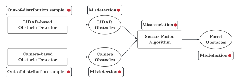
Figure 1: Perception system including 3 modules (rectangles) and 3 outputs (circles). Modules are connected by edges describing which module produces or consumes a given output. The failure modes of each module (resp. output) are represented by red dots.

Remark 2 (Modules vs. Outputs).

Our system model treats modules and outputs as separate nodes. This is convenient for two reasons. First, fault identification at the modules and outputs may serve different purposes: output fault identification is more useful at runtime to identify unreliable information from the perception system and prevent accidents; module fault identification is typically more informative for designers and regulators. Second, in practical applications we can rarely measure if a module is failing (indeed developing algorithms that can “self-diagnose” their failures is an active area of research, see work on certifiable algorithms [73]). On the other hand, we can directly measure the outputs of the modules and develop diagnostic tests to check if an output is plausible and consistent with other outputs in the system.

3.2 Fault Detection and Fault Identification

Each module in ${\cal S}$ might fail at some point, jeopardizing the system performance or even its safety. In particular, each module $m\in{\cal M}$ is assumed to have a set of failure modes. While the list of failures can include any software and hardware failures, in this paper we particularly focus on failures of the intended functionality. For example, a neural-network-based camera-based object detection module might experience the failure mode “out-of-distribution sample” when it processes an input image, which indicates that while the module’s code executed successfully, the resulting detection is expected to be incorrect.

Similarly, each output $o\in{\cal O}$ has an associated set of failure modes. For instance, the output of the camera-based object detector might experience a “mis-detection” failure mode if it fails to detect an object, or a “mis-classification” failure mode if the object is detected but misclassified. A module’s failure mode typically causes a failure in one of its outputs. Examples of failure modes are given in Fig. 1. For each module and output, the figure lists a potential failure mode: for instance, the LiDAR-based obstacle detection output may fail if it misdetects an obstacle, while the sensor fusion module may fail it it incorrectly associates the input obstacles.

Definition 3 (Failure Modes).

At each time instant, the $i$-th failure mode $f_{i}\in\{\mathrm{INACTIVE},\mathrm{ACTIVE}\}\cong\{0,1\}$ is either ACTIVE (also $1$) if such failure is occurring, or INACTIVE (also $0$). A module or an output is failing if at least one of its failure modes is ACTIVE. If we stack the status (ACTIVE/INACTIVE) of all failure modes into a single binary vector, the fault state vector ${\bm{f}}\in\{0,1\}^{N_{f}}$ (where ${N_{f}}$ is the number of failure modes), then ${\bm{f}}$ is all zeros if there are no faults, or has entries equal to ones for the active failure modes.

The goal of this paper is then to address the following problems:

Fault Detection

decide whether the system is working in nominal conditions or whether a fault has occurred (i.e., infer if there is at least an active failure mode in ${\bm{f}}$);

Fault Identification

identify the specific failure mode the system is experiencing (i.e., infer which failure mode is active in ${\bm{f}}$).

Fault detection is the easiest between the two problems, as it only requires specifying the presence of at least a fault, without specifying which modules or outputs are incorrect. Mathematically, this reduces to identifying whether the unknown vector ${\bm{f}}$ has at least an entry equal to $1$. Fault identification goes one step further by explicitly indicating the set of active failure modes. Mathematically, this reduces to identifying exactly which entries of the unknown vector ${\bm{f}}$ are equal to $1$. Identifying which module is faulty is particularly important to inform regulators (e.g., to trace the steps that that led to an accident caused by an autonomous vehicle) and system designers (e.g., to highlight modules that are likely to fail and require further development). Moreover, not all faults are equally problematic: for instance, a failure in localizing a car in the opposite lane of a divided highway is less consequential that failing to detect a pedestrian in front of the car. Note that solving fault identification implies a solution for fault detection (i.e., whenever we declare one or more modules to be faulty, we essentially also detected there is a failure), hence in the rest of this paper we focus on the design of a monitoring system for fault identification.

Remark 4 (Assumptions and Terms of Use).

We assume that the potential failure modes of the system are known to the system designer. In practice, these can be discovered using some form of hazard analysis, such as Failure Modes and Effects Analysis (FMEA) [74] or Fault tree analysis (FTA) [75]. Moreover, one can always add a generic “unknown failure mode” to the list of failure modes of a module or output, hence this assumption is not restrictive. We also remark that our monitoring system’s objective is to diagnose potential failures, while it does not prescribe what are the actions that need to be taken in response to each failure (e.g., whether to stop the car, provide a warning to the passenger, etc.), which is failure and system-dependent. Investigation how to respond to or mitigate failures is left to future work.

4 Modeling Fault Identification with Diagnostic Graphs

This section develops a framework to model fault identification problems in perception systems. In the previous section we have discussed how the goal is to identify the set of active failure modes associated to modules and outputs in a system. Here we introduce the concept of diagnostic graphs to study fault identification: diagnostic graph will allow developing fault identification algorithms (Section 5) and understanding fundamental limits (Section 6).

The intuition is that in a perception system we can perform a number of diagnostic tests that check the validity of the output of certain modules. For instance, we can compare the outputs of different modules to ensure they are consistent (e.g., compare the obstacles detected by the LiDAR-based obstacle detection against the camera-based obstacle detection), or inspect that the output a certain module respects certain requirements (e.g., the vision-based ego-motion module is tracking a sufficient number of features). Then, we can model these checks as edges in a bipartite graph, the diagnostic graph, which can be used for fault identification. In the following, we formalize the notions of diagnostic tests and diagnostic graphs.

4.1 Diagnostic Tests

In our fault identification framework, the system is equipped with a set of diagnostic tests that can (possibly unreliably) provide diagnostic information about the state of a subset of failure modes. Each diagnostic test is a function $t:\mathbb{S}\to\{\mathrm{PASS},\mathrm{FAIL}\}$, where $\mathbb{S}\subseteq\{1,\ldots,{N_{f}}\}$ is a subset of the failure modes that the test is checking, called the scope of the test, and the test returns a value $z\in\{\mathrm{PASS},\mathrm{FAIL}\}\cong\{0,1\}$, called the outcome of the test. A diagnostic test returns PASS (also denoted with $0$) if there is no active failure mode in its scope, FAIL (also denoted with $1$) otherwise. In general, tests can be unreliable, meaning that they can both fail to detect active failures or incorrectly detect failures as active (i.e., false alarms).

While in the experimental section we will describe more complex tests (and provide an open-source framework to easily code new tests), it is instructive to consider a simple test between the outputs of the LiDAR-based obstacle detection and the camera-based obstacle detection in Fig. 3. The test in Fig. 3 compares the two sets of objects detected by the two detectors; whenever an inconsistency arises, the test returns FAIL. However, if both detectors are subject to the same failure, e.g., they both misdetect an obstacle, the test might still pass, thus exhibiting unreliable behavior. We remark that a single test does not suffice for fault identification: for instance, if the test in Fig. 3 fails, we can only conclude that one of the two detectors had a failure (or that the test was a false alarm); therefore, we typically need to collect a number of tests and perform some inference process to draw conclusions about which modules failed. The collection of the outcomes of multiple diagnostic tests is called a syndrome.

Definition 5 (Syndrome).

Assuming we have ${N_{t}}$ diagnostic tests, the vector collecting the test outcomes ${\bm{z}}\in\{\mathrm{PASS},\mathrm{FAIL}\}^{N_{t}}$ is called a syndrome.

In the following, we describe how to mathematically model the relation between the failure modes and the test outcomes; this will be instrumental in solving the inverse problem of identifying the failure mode from a given syndrome. We provide a deterministic and a probabilistic model for the tests below.

Deterministic Tests. Deterministic diagnostic tests encode the set of possible test outcomes, by establishing a deterministic relation between failure modes in the test’s scope and the test outcome. We discuss potential models for deterministic diagnostic test below.

Ideally we would like the test to return FAIL if and only if at least one of the failure modes in its scope is active. This leads to the definition of a “Deterministic OR” test.

Definition 6 (Deterministic OR).

A diagnostic test $t({\bm{f}}_{\operatorname{scope}(t)})$ is a deterministic OR if its test outcome $z$ is

$$z=\begin{cases}\mathrm{PASS}&\text{if }\|{\bm{f}}_{\operatorname{scope}(t)}\|_{1}=0\\ \mathrm{FAIL}&\text{otherwise}\end{cases}$$ (1)

This kind of tests can be hard to implement in practice. For example, imagine a diagnostic test that compares the output of two object classifiers: if one of them produces a wrong label, it is easy to detect there is a failure; however, if both classifiers are trained on similar data and both report the incorrect label there is no way to detect the failure. In this case, the test outcome is unreliable. The following definition introduces a type of unreliable test.

Definition 7 (Deterministic Weak-OR).

A test $t({\bm{f}}_{\operatorname{scope}(t)})$ is a deterministic Weak-OR if its test outcome $z$ is

$$z=\begin{cases}\mathrm{PASS}&\text{if }0<\|{\bm{f}}_{\operatorname{scope}(t)}\|_{1}<|\operatorname{scope}(t)|\\ \mathrm{PASS}\text{ or }\mathrm{FAIL}&\text{if }\|{\bm{f}}_{\operatorname{scope}(t)}\|_{1}=|\operatorname{scope}(t)|\\ \mathrm{FAIL}&\text{otherwise}\end{cases}$$ (2)

This kind of test is consistent with the tests used in [76]. Intuitively, a “Deterministic Weak-OR” may return PASS even if all failure modes are active, since the test might fail to detect an inconsistency if all faults are consistent with each others (again, think about two object classifiers failing in the same way). Even though the Weak-OR test may pass or fail when all failure modes are active, its outcome remains deterministic.

Finally, an even weaker type of deterministic test is what we call the Deterministic Weaker-OR (this is the easiest test to implement in practice).

Definition 8 (Deterministic Weaker-OR).

A diagnostic test $t({\bm{f}}_{\operatorname{scope}(t)})$ is a Deterministic Weaker-OR if its test outcome $z$ is

$$z=\begin{cases}\mathrm{PASS}\text{ or }\mathrm{FAIL}&\text{if }\|{\bm{f}}_{\operatorname{scope}(t)}\|_{1}>0\\ \mathrm{PASS}&\text{if }\|{\bm{f}}_{\operatorname{scope}(t)}\|_{1}=0\\ \end{cases}$$ (3)

In other words, the tested is designed to pass in nominal conditions (i.e., when no failure mode is active), but it can have arbitrary outcomes otherwise.

The types of deterministic tests presented above are not the only possible deterministic tests. Other examples include, for instance, diagnostic tests that fail to detect specific sets of failure modes. Deterministic tests can be designed using formal methods tools or certifiable perception algorithms [77, 78, 79], see also Remark 10 below.

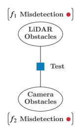
[] Scope Test outcome $z$ $f_{1}$ $f_{2}$ OR Noisy-OR $0$ $0$ $\quad 0\quad$ $\left\{\begin{array}[]{ll}0\text{ with prob. }(1-p_{a,1})(1-p_{a,2})\\ 1\text{ with prob. }p_{a,1}+p_{a,2}-p_{a,1}p_{a,2}\end{array}\right.$ $0$ $1$ $1$ $\left\{\begin{array}[]{ll}0\text{ with prob. }(1-p_{a,1})(1-p_{d,2})\\ 1\text{ with prob. }p_{a,1}+p_{d,2}-p_{a,1}p_{d,2}\end{array}\right.$ $1$ $0$ $1$ $\left\{\begin{array}[]{ll}0\text{ with prob. }(1-p_{d,1})(1-p_{a,2})\\ 1\text{ with prob. }p_{d,1}+p_{a,2}-p_{d,1}p_{a,2}\end{array}\right.$ $1$ $1$ $1$ $\left\{\begin{array}[]{ll}0\text{ with prob. }(1-p_{d,1})(1-p_{d,2})\\ 1\text{ with prob. }p_{d,1}+p_{d,2}-p_{d,1}p_{d,2}\end{array}\right.$

Figure 2: A test comparing two outputs, LiDAR Obstacles and Camera Obstacles

Figure 3: Table of possible outcomes for the Deterministic OR and the probabilistic Noisy-OR version of a test with scope $f_{1}$ and $f_{2}$.

Probabilistic Tests. Deterministic tests might not capture the complexity of real world diagnostic tests. Most practical tests are likely to incorrectly detect faults (i.e., produce false positive) or fail to detect faults (i.e., produce false negatives) with some probability. For this reason, in this paper, we also allow for an arbitrary probabilistic relationship between test outcomes and failure modes in the test scope.

A simple-yet-expressive way to formalize a probabilistic test is to use what we call a “Noisy-OR” model. In particular, the Noisy-OR model represents the probability of a diagnostic test outcome as a conditional probability distribution over the failure modes in its scope $\Pr(z\mid{\bm{f}}_{\operatorname{scope}(t)})$ as defined below.

Definition 9 (Noisy-OR).

A diagnostic test $t({\bm{f}}_{\operatorname{scope}(t)})$ is a probabilistic Noisy-OR if its test outcome $z$ follows

$$\Pr(z=\mathrm{PASS}\mid{\bm{f}}_{\operatorname{scope}(t)})= \prod_{i\in\operatorname{scope}(t)}\Pr(z=\mathrm{PASS}\mid f_{i})$$ (4)

where $\Pr(z\mid f_{i})$ denotes the conditional probability of the test outcome (PASS/FAIL) conditioned on the status (ACTIVE/INACTIVE) of the failure mode $f_{i}$. Clearly, $\Pr(z=\mathrm{FAIL}\mid{\bm{f}}_{\operatorname{scope}(t)})=1-\Pr(z=\mathrm{PASS}\mid{\bm{f}}_{\operatorname{scope}(t)})$.

Now suppose each test has a probability $p_{d,i}$ of correctly identifying failure $f_{i}$ (detection probability), and a probability $p_{a,i}$ of false alarm for $f_{i}$. Exploiting the fact that $f_{i}\in\{0,1\}$, we can write Eq. 4 as:

$$\Pr(z=\mathrm{PASS}\mid{\bm{f}}_{\operatorname{scope}(t)})=\prod_{i\in\operatorname{scope}(t)}(1-p_{d,i})^{f_{i}}(1-p_{a,i})^{1-f_{i}}$$ (5)

An example of probabilistic test outcome is given in Fig. 3.

Similarly to the deterministic case, the Noisy-OR model is not the only possible model. However, Section 7 shows that this model is particularly effective in modeling fault identification problems in practice. In Section 5, we discuss how to learn the probabilities involved in probabilistic tests (i.e., $p_{d,i}$ and $p_{a,i}$ in Eq. 5) given a training dataset, and how to use the test outcomes to infer the most likely failure modes. Towards that goal, we need to group diagnostic tests into a suitable graph structure, called a diagnostic graph, which we present in the following section. We conclude this section with a remark.

Remark 10 (From diagnostic tests to fault identification).

The diagnostic tests we introduced in this section are not dissimilar from the typical diagnostic tests or watchdogs considered in prior work or used by practitioners. Our goal here is to formalize these tests and use the test outcomes to infer the most likely set of system-wide failures. In this sense, our fault identification framework is designed to capitalize on (rather than replace) existing diagnostic tools used in practice. For example the detection mechanism proposed by Liu and Park [55], which is based on the idea of projecting the 3D LiDAR points onto camera images, and then checking whether objects detected from LiDAR and images match each other, can be formulated as a diagnostic tests with the camera and LiDAR misdetection in its scope, such that the test outcome is the output of the algorithm in [55]. Also, out-of-distribution detection based on epistemic uncertainty, e.g., [56], can be formulated as a diagnostic tests with the module’s “out-of-distribution sample” failure mode in its scope, such that the test outcome is FAIL if the estimated uncertainty is above a threshold.

4.2 Diagnostic Graph

A diagnostic graph is a structure defined over a perception system and has the goal of describing the diagnostic tests (as well as more general relations among failure modes) and their scope. We provide a formal definition below.

Definition 11 (Diagnostic Graph).

A diagnostic graph is a bipartite graph ${\cal D}=({\cal V},{\cal R},{\cal E})$ where the nodes are split into variable nodes ${\cal V}$, corresponding to the failure modes in the system, and relation nodes ${{\cal R}}$, where each relation $\phi_{k}({\bm{f}})\in{\cal R}$ is a function over a subset of failure modes ${\bm{f}}$. Then an edge in ${\cal E}$ exists between a failure mode $f_{i}\in{\cal V}$ and a relation $\phi_{k}\in{\cal R}$, if $f_{i}$ is in the scope of the relation $\phi_{k}$ (i.e., if the variable $f_{i}$ appears in the function $\phi_{k}$).

Relations capture constraints among the variables induced by the test outcomes or from prior knowledge we might have about the failure modes. We describe the two main types of relations below and for each we describe their implementation in the deterministic and probabilistic case.

Definition 12 (Test-driven Relations).

A test-driven relation $\phi_{k}$ describes whether —for a test $t_{k}$— a given set of failure mode assignments might have produced a certain test outcome $z_{k}$. More formally, for a deterministic test $t_{k}$, a test-driven relation is a boolean function:

$$\phi_{k}({\bm{f}})=\phi({\bm{f}}_{\operatorname{scope}({t_{k}})};z_{k})=\operatorname{\mathds{1}}\left[z_{k}=t\left({\bm{f}}_{\operatorname{scope}({t_{k}})}\right)\right]$$ (6)

where $\operatorname{\mathds{1}}$ is the indicator function that returns $1$ if the condition is satisfied or $0$ otherwise. The function Eq. 6 checks if an assignment of failure modes ${\bm{f}}$ may have produced the test outcome $z_{k}$ and where the notation $\phi_{k}({\bm{f}})=\phi({\bm{f}}_{\operatorname{scope}({t_{k}})};z_{k})$ clarifies that the function $\phi_{k}$ only involves a subset of failure modes ${\bm{f}}_{\operatorname{scope}({t_{k}})}$ (the ones in the scope of test $t_{k}$) and depends on the (given) test outcome $z_{k}$. Similarly, for a probabilistic test $t_{k}$, a test-driven relation is a real-valued function:

$$\phi_{k}({\bm{f}})=\phi({\bm{f}}_{\operatorname{scope}({t_{k}})};z_{k})=\Pr(z_{k}|{\bm{f}}_{\operatorname{scope}(t_{k})})$$ (7)

which returns the likelihood of the test outcome $z_{k}$ given an assignment ${\bm{f}}$.

Definition 13 (A Priori Relations).

An a priori relation describes whether a given set of failure modes is plausible, considering a priori knowledge about the system. More formally, in the deterministic case, an a priori relation is a boolean function $\phi_{k}({\bm{f}})$ that returns $1$ if the assignment of ${\bm{f}}$ is plausible or $0$ otherwise. Similarly, in the probabilistic case, an a priori relation is a real-valued function $\phi_{k}({\bm{f}})$ that returns the likelihood of a given assignment ${\bm{f}}$.

In the following we will denote the set of Test-driven Relations as ${\cal R}_{\mathrm{test}}$ while the set of A Priori Relations as ${\cal R}_{\mathrm{prior}}$. Therefore, ${\cal R}={\cal R}_{\mathrm{test}}\cup{\cal R}_{\mathrm{prior}}$.

While we have provided several examples of diagnostic tests in the previous section, we now provide examples of a priori relations. For instance, in the deterministic case, some failure modes of a module can be mutually exclusive (e.g., “too many outliers”, “not enough features” in the Lidar-based ego-motion estimation) or one can imply another (e.g., if a module is experiencing an “out-of-distribution sample” failure mode, then its outputs will have at least an active failure mode). Not all relations are deterministic, for example in Fig. 4, the failure modes of the sensor fusion algorithm may have a complex probabilistic relationship with the failure modes of the lidar and camera obstacles failure modes. Note that the main difference between test-driven relations and a priori relations is that the former provides a measurable test outcome, while the latter relies on a priori knowledge about the system (i.e., no outcome is measured).

We elucidate on the notion of diagnostic graph with two examples below. Example 1: Multi-sensor Obstacle Detection. Consider the perception system in Fig. 1. We can associate a diagnostic graph to the system where the variable nodes of the diagnostic graph are the failure modes of modules and outputs in the system. The diagnostic graph, shown in Fig. 4, also includes two diagnostic tests and a priori relations encoding input/output relationship between modules and outputs. Each diagnostic test compares a pair of outputted obstacles, namely LiDAR obstacles and camera obstacles (with failures $f_{4}$ and $f_{5}$), and camera obstacles and fused obstacles (with failures $f_{4}$ and $f_{6}$).

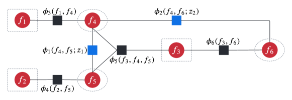
Figure 4: A diagnostic graph for the perception system example in Fig. 1. Red circles represent variable nodes (failure modes) while squares represent relations. Test-driven Relations are shown in blue, while a priori relations are shown in black.

Example 2: LiDAR-based Ego-motion Estimation. We provide a second example that also includes singleton diagnostic tests (having a single failure mode in their scope) and includes explicit tests over modules. The example consists of a LiDAR-based odometry system that computes the relative motion between consecutive LiDAR scans using feature-based registration, see e.g., [80, 81]. The system ${\cal S}$ comprises two modules, a feature extraction module and a point-cloud registration module, as depicted in Fig. 5(left). The feature extraction module extracts 3D point features from input LiDAR data, while the point-cloud registration module uses the features to estimate the relative pose between two consecutive LiDAR scans. Suppose that the feature extraction module is based on a deep neural network and that it can experience an “out-of-distribution sample” failure, which causes the corresponding output to potentially experience “too-many outliers” or “few features” failures. Similarly, the module point-cloud registration can experience the failure “suboptimal solution”, which leads its outputs, the relative pose, to experience a “wrong relative pose” failure. Fig. 5(right) shows a diagnostic graph for the system. The system is equipped with three diagnostic tests. A diagnostic test detects if the failure mode “few features” is active by checking the cardinality of the feature set. If the point-cloud registration module is a certifiable algorithm [73], we can attach a diagnostic test to the point-cloud registration module that uses the module’s certificate to detect if the module is experiencing a “suboptimal solution” failure. Another diagnostic test detects if the relative pose is wrong by checking that the relative pose does not exceed some meaningful threshold given the vehicle dynamics. Finally, another test checks if under the computed relative pose, the feature extractor has “too many outliers”. This can be achieved by counting the number of features that are correctly aligned after applying the estimated relative pose. The diagnostic graph also contains a priori relations encoding constraints on the input/output relationships.

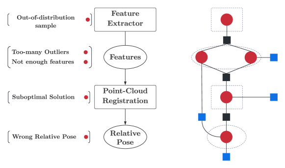
Figure 5: (Left) Example of the LiDAR-based ego-motion estimation system ${\cal S}$. The system is composed by two modules (rectangles), each producing one output (circles). (Right) The corresponding diagnostic graph, where red circles represent variable nodes (failure modes) while squares represent relations (test-driven Relations in blue, a priori relations in black).

4.2.1 Temporal Diagnostic Graph

So far, we have considered a diagnostic graph as a representation of the diagnostic information available at a specific instant of time (e.g., the examples above include tests and relations involving the behavior of modules and outputs at a certain time instant). However, perception systems evolve over time, and considering the temporal dimension offers further opportunities for fault identification, e.g., by monitoring the temporal evolution of the outputs.

Suppose we have a collection of diagnostic graphs ${\cal T}=\{{\cal D}^{(t)},\ldots,{\cal D}^{(t+K)}\}$, collected over and interval of time. We could think of stacking these diagnostic graphs, into a new temporal diagnostic graph ${\cal D}^{[K]}$. The temporal graph preserves the failure mode, relations and edges of each sub-graph ${\cal D}^{(k)}\in{\cal T}$. However, since ${\cal D}^{[K]}$ includes outputs produced at multiple time instants, we can also augment the graph to include temporal diagnostic tests and temporal relationships. For example, we might check that an obstacle does not disappear from the scene (unless it goes out of the sensor field of view), or that the pose of the ego-vehicle does not change too much over time. As we will see, the use of temporal diagnostic graph leads to slightly improved fault identification performance. An example of temporal diagnostic graph is given in Fig. 6.

The algorithms and results presented in the rest of this paper apply to both regular and temporal diagnostic graph, unless specified otherwise.

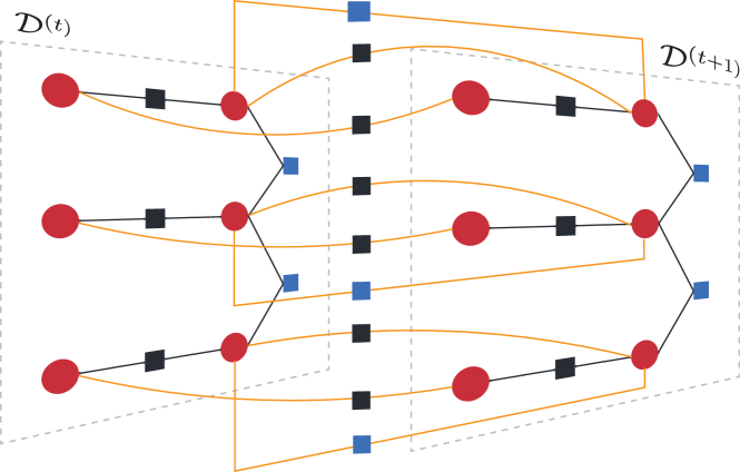
Figure 6: Example of Temporal Diagnostic Graph composed by two identical sub-graphs. We added temporal relations (both test-driven and a priori) between the two sub-graphs.

Remark 14 (Temporal Diagnostic Tests).

Temporal diagnostic tests are used to monitor the evolution of the system over time. For example the Timed Quality Temporal Logic in [45] can be implemented with a temporal diagnostic test that spans multiple ${\cal D}^{(t)}$’s. More specifically, the test example considered in [45] requires that “At every time step, for all the objects in the frame, if the object class is cyclist with probability more than $0.7$, then in the next $5$ frames the same object should still be classified as a cyclist with probability more than $0.6$”. This can be modeled as a diagnostic test that spans $5$ diagnostic graphs and that returns FAIL if the predicate is false.

5 Algorithms for Fault Identification

This section shows how to perform fault identification over a diagnostic graph. In particular, we present algorithms to infer which failure modes are active, given a syndrome. We study fault identification with deterministic tests in Section 5.1 and then extend it to the probabilistic case in Section 5.2. Finally, we present a graph-neural-network approach for fault identification in Section 5.3.

5.1 Inference in the Deterministic Model

In the deterministic case, our inference algorithm looks for the smallest set of active failure modes that explains a given syndrome. In Section 6, we will show that such approach is guaranteed to correctly identify the faults as long as the tests provide a sufficient level of redundancy, an insight we will formalize through the notion of “diagnosability”.

Looking for the smallest set of active failures that explains the test outcomes (and more generally, the relations) in a diagnostic graph can be formulated as the following optimization problem (given a syndrome ${\bm{z}}$):

$$\underset{{\bm{f}}\in\{0,1\}^{N_{f}}}{\textrm{minimize}} \|{\bm{f}}\|_{1}$$ (D-FI)

subject to $$\phi_{k}({\bm{f}}_{\operatorname{scope}(t_{k})};z_{k})=1, i=1,\ldots,{N_{t}},$$

$$\phi_{j}({\bm{f}})=1, j=1,\ldots,N_{r},$$

where $\phi_{k}({\bm{f}}_{\operatorname{scope}(t_{k})};z_{k})$ are the ${N_{t}}$ test-driven relations in the diagnostic graph, while $\phi_{j}({\bm{f}})$ are the $N_{r}$ a priori relations in the graph. In words, Eq. D-FI looks for binary decisions (ACTIVE/INACTIVE) for the failure modes ${\bm{f}}$, and looks for the smallest set of faults (the objective $\|{\bm{f}}\|_{1}$ counts the number of ACTIVE failure modes) such that the faults satisfy the relations in the diagnostic graph. Eq. D-FI is our Deterministic Fault Identification algorithm.

The optimization in Eq. D-FI can be solved using standard computational tools from Integer Programming [82] or Constraint Satisfaction Programming [83]. While integer programming is better suited to find the solution to the minimization problem, constraint programming also allows finding all the solutions in the feasible set. The choice between the two depends on the application and the expression for the relations. In our experiments, we solve it using Integer Programming. We remark that while Integer Programming is NP complete, our problems typically only involve tens to hundreds of failure modes, and can be solved efficiently in practice.

The model presented above is generic and valid for any deterministic test and a priori relations. In the following, we provide an example to ground the discussion and show how to instantiate the optimization problem in practice.

Example 3: Deterministic Inference with Weaker-OR and Module-Output Relations. We consider a diagnostic graph with Deterministic Weaker-OR tests. Moreover, as a priori relations, we assume that whenever the output of a module has a failure, then also the module itself must have at least an active failure mode. This is also the setup we use in our experiments in Section 7.

In Weaker-OR diagnostic tests, the PASS outcome is unreliable, meaning that if a test returns PASS it might have $0$ or more failure modes active in its scope. However, when it the test returns FAIL, we know there must be at least one failure mode active. This can be easily enforced in the optimization by imposing the constraint:

$$\|{\bm{f}}_{\operatorname{scope}(t_{i})}\|_{1}\geq 1\qquad\forall t_{i}\in\{1,\ldots,{N_{t}}\}\text{ such that }z_{i}=\mathrm{FAIL},$$

We then have to enforce the relation that if an output has an active failure mode, then the module that produced it must have at least one active failure mode as well. Towards this goal, let ${\cal F}(o_{i})\subseteq\{1,\ldots,{N_{f}}\}$ be the set of failure modes associated to outputs of module $m_{i}$ and ${\cal F}(m_{i})$ be the set of failure modes associated to $m_{i}$; then the a priori relation can be enforced via the constraint:

$$\|{\bm{f}}_{{\cal F}(m_{i})}\|_{1} \geq\frac{1}{|{\cal F}(o_{i})|}\|{\bm{f}}_{{\cal F}(o_{i})}\|_{1}$$

Intuitively, when there is no active failure in the outputs (i.e., $\|{\bm{f}}_{{\cal F}(o_{i})}\|_{1}=0$) the constraint is trivially satisfied, while when there is at least an output failure (i.e., $\|{\bm{f}}_{{\cal F}(o_{i})}\|_{1}>0$) then $\|{\bm{f}}_{{\cal F}(m_{j})}\|_{1}$ is forced to be at least $1$. The resulting optimization problem finally becomes:

$$\underset{{\bm{f}}\in\{0,1\}^{N_{f}}}{\textrm{minimize}} \|{\bm{f}}\|_{1}$$ (8)

subject to $$\|{\bm{f}}_{\operatorname{scope}(t_{i})}\|_{1}\geq 1\qquad\forall t_{i}\in\{1,\ldots,{N_{t}}\}\text{ such that }z_{i}=\mathrm{FAIL},$$

$$\|{\bm{f}}_{{\cal F}(m_{i})}\|_{1}\geq\frac{1}{|{\cal F}(o_{i})|}\|{\bm{f}}_{{\cal F}(o_{i})}\|_{1}\qquad\forall m_{i}\in{\cal M}.$$

5.2 Inference in the Probabilistic Model

This section shows how to use the formalism of factor graphs to find the most likely active failure modes that explain a given syndrome in a diagnostic graph with probabilistic tests.

Factor graphs are a powerful class of probabilistic graphical models. Probabilistic graphical models allow describing relationships between multiple variables using a concise language. In particular, they describe joint or conditional distributions over a set of unknown variables and a set of known observations, and can be used to infer the values of the unknown variables. In this work we limit ourselves to factor graphs over discrete (binary) variables. We start from the definition of a factor graph.

Definition 15 (Factor Graph).

A factor graph is a bipartite graph $F=({\cal V},\Phi,{\cal E})$ consisting of a set ${\cal V}$ of variable nodes, a set $\Phi$ of factor nodes, and a set ${\cal E}\subseteq{\cal V}\times\Phi$ of edges having one endpoint at a variable node and the other at a factor node. Let $\operatorname{{\cal N}}(\phi)$ the set of variables to which a factor node $\phi$ is connected, then, the factor graph defines a family of distributions that factorize according to

$$\mu({\bm{f}}\mid{\bm{z}})=\frac{1}{Z}\prod_{\phi\in\Phi}\phi({\bm{f}}_{\operatorname{{\cal N}}(\phi)};{\bm{z}})$$ (9)

where the normalization factor $Z$, also known as the partition function, ensures that $\mu({\bm{f}})$ is a valid distribution:

$$Z({\bm{z}})=\sum_{{\bm{f}}}\prod_{\phi\in\Phi}\phi({\bm{f}}_{\operatorname{{\cal N}}(\phi)};{\bm{z}})$$ (10)

The notation $\phi({\bm{f}}_{\operatorname{{\cal N}}(\phi)};{\bm{z}})$ emphasizes the fact that each factor is a function of a subset ${\bm{f}}_{\operatorname{{\cal N}}(\phi)}$ of the failure modes ${\bm{f}}$, for given observed ${\bm{z}}$.

The factor graph $F$ and the diagnostic graph ${\cal D}$ have a similar structure. In fact we can choose the set of variables ${\cal V}$ in the factor graph to be the same as the set of variables in the diagnostic graph, namely the set of failure modes. Then, we can choose the set of factors $\Phi$ to be the relations ${\cal R}$ of ${\cal D}$, and the set of edges to be the same. Therefore, for a given diagnostic graph ${\cal D}$, it is easy to devise the corresponding factor graph as:

$$\mu({\bm{f}}\mid{\bm{z}})=\frac{1}{Z}\prod_{\phi_{k}\in{\cal R}_{\mathrm{test}}}\phi_{k}({\bm{f}}_{\operatorname{scope}(t_{k})};z_{k})\prod_{\phi_{j}\in{\cal R}_{\mathrm{prior}}}\phi_{j}({\bm{f}}_{\operatorname{{\cal N}}(\phi_{j})})$$ (11)

where we have simply observed that the probability distributions induced by the relations in the diagnostic graph naturally factorize into factors, each one corresponding to a (test-driven or a priori) relation in the diagnostic graph.

Maximum a Posteriori Inference. Given a factor graph, a natural question to ask is what is the most likely assignment of variables that maximizes the probability distribution induced by the factor graph (e.g., in our case, this is the most likely set of faults in the system). This leads to the concept of maximum a posteriori (MAP) inference, which —given a factor graph and a syndrome ${\bm{z}}$— looks for the most likely variables ${\bm{f}}^{\star}$, that maximize the posterior distribution:

$${\bm{f}}^{\star}=\operatorname*{arg\,max}_{{\bm{f}}\in\{0,1\}^{N_{f}}}\;\mu({\bm{f}}\mid{\bm{z}})$$ (FG-FI)

Computing a MAP estimate is known to be NP-hard for general factor graphs [84], therefore it is common to use approximate methods. In our experiments we used belief propagation(Sec. 3 in [85]) to solve the MAP inference, which finds the optimal solution for tree-structured factor graphs, and is known to empirically return good approximations for the MAP estimate in general factor graphs.

Learning the Factor Graph Parameters. While in the deterministic case we know the expression of the relations $\phi_{k}$, in the probabilistic case the probabilistic tests might depend on unknown parameters, cf. the expression in Eq. 5 that requires specifying the parameters $p_{d,i}$ (probability that a fault is not detected) and $p_{a,i}$ (probability of a false alarm). There are several paradigms to learn the factor graph parameters. In our experiments we use a method called structured support vector machine (SSVM) or maximum margin learning (Sec. 19.7 in [86]).

5.3 Graph Neural Networks for Fault Identification

The factor graph framework introduced in the previous section learns the factor graph parameters from training data, and then performs maximum a posteriori inference at runtime for fault identification. In this section, we propose a learning-based framework that is also trained on a dataset, but then learns directly how to predict which failure mode is active at runtime. In particular, we use Graph Neural Networks (GNN) to learn to identify active faults in a diagnostic graph.

GNNs provide a general framework for learning using graph-structured data, and have empirically achieved state-of-the-art performance in many tasks such as node classification, link prediction, and graph classification [87]. The fault identification problem considered in this paper can be phrased as a node classification problem. In node classification, given a undirected graph $G=({\cal V},{\cal E})$ where each node $i\in{\cal V}$ has an (unknown) label $y_{i}$, the objective is to learn a representation vector ${\bm{e}}_{i}$ of node $i$ such that label $y_{i}$ can be predicted as a function of the node embeddings ${\bm{e}}_{i}$.

In the following, we recall common GNN architectures (Section 5.3.1) and then we discuss how to transform our diagnostic graph into a structure that can be fed to a GNN to predict active faults (Section 5.3.2).

5.3.1 Graph Neural Network Preliminaries

A GNN is an extension of recurrent neural networks that operates on graph-structured data. GNNs are based on the concept of neural message passing in which real-valued vector messages are exchanged between nodes of a graph —not dissimilarly to the belief propagation we used in Section 5.2— but were the messages (and node updates) are built using differentiable functions encoded as neural networks. To understand the basic idea of neural message passing consider an undirected graph $G=({\cal V},{\cal E})$. At the beginning, each node is assigned a feature vector ${\bm{e}}_{i}^{(0)}$ for each $i\in{\cal V}$. Then, during each message-passing iteration $k=1,2,\ldots$, the embedding ${\bm{e}}_{i}^{(k)}$ is updated by aggregating the embeddings of node $i$’s neighborhood $\operatorname{{\cal N}}(i)$

$${\bm{e}}_{i}^{(k+1)} =\operatorname{update}\left({\bm{e}}_{i}^{(k)},\operatorname{aggregate}\left(\left\{{\bm{e}}_{j}^{(k)}\;\mid\;j\in\operatorname{{\cal N}}(i)\right\}\right)\right)$$ (12)

$$=\operatorname{update}\left({\bm{e}}_{i}^{(k)},{\bm{a}}_{i}^{(k)}\right)$$ (13)

Where $\operatorname{aggregate}({\cdot})$ and $\operatorname{update}({\cdot})$ are two learned differentiable functions (i.e., neural networks). At each iteration $k$, the $\operatorname{aggregate}({\cdot})$ function takes the embeddings of node $i$’s neighbors and generates a message ${\bm{a}}_{i}^{(k)}$. Then, the $\operatorname{update}({\cdot})$ function combines the message with the previous embedding of node $i$, generating the new embedding of node $i$. The final embedding is obtained by running the neural message passing for $K$ iterations. Finally, the node label is predicted by a learned differentiable function of the node embeddings:

$$y_{i}=\operatorname{\mathrm{READOUT}}({\bm{e}}_{i}^{(K)})$$ (GNN-FI)

The literature on GNN offers a number of potential choices for the $\operatorname{update}({\cdot})$ and $\operatorname{aggregate}({\cdot})$ functions. We review four popular choices below.

Graph Convolutional Networks (GCNs). One of the most popular graph neural network architectures is the graph convolutional network (GCN) [88]. The GCN model implements the update and aggregate function as:

$${\bm{e}}_{i}^{(k+1)}=\sigma\left({\bm{W}}^{(k+1)}\sum_{j\in\operatorname{{\cal N}}(i)\cup\{i\}}\frac{{\bm{e}}_{j}^{(k)}}{\sqrt{|\operatorname{{\cal N}}(i)||\operatorname{{\cal N}}(j)|}}\right)$$ (14)

where ${\bm{W}}^{(k+1)}$ is a trainable weight matrix and $\sigma(\cdot)$ is a nonlinear activation function. Note that Eq. 14 can also be written in a matrix form

$${\bm{E}}^{(k+1)}=\sigma\left(\hat{{\bm{P}}}{\bm{E}}^{(k)}{\bm{W}}^{(k+1)}\right)$$

where $\hat{{\bm{P}}}=\hat{{\bm{D}}}^{-\frac{1}{2}}({\bm{A}}+{\mathbf{I}})\hat{{\bm{D}}}^{-\frac{1}{2}}$, the matrix ${\bm{A}}$ is the adjacency matrix of the original graph, and $\hat{{\bm{D}}}$ is its diagonal degree matrix.

Graph Convolutional Network via Initial residual and Identity mapping (GCNII). The GCN is affected by the over-smoothing problem [89], where after several iterations of GNN message passing, the nodes’ embeddings become very similar to each another; over-smoothing prevents the use of deeper GNN models, which in turn prevents the GNN from leveraging longer-term dependencies in the graph. To solve this problem, Chen et al. [90] propose the GCNII, where the update of the embedding vectors becomes:

$${\bm{E}}^{(k+1)}=\sigma\left(\left((1-\alpha_{k})\hat{{\bm{P}}}{\bm{E}}^{(k)}+\alpha_{k}{\bm{E}}^{(0)}\right)\left((1-\beta_{k}){\mathbf{I}}+\beta_{k}{\bm{W}}^{(k)}\right)\right)$$ (15)

and where $\alpha_{k}$ and $\beta_{k}$ are two hyper-parameters. GCNII improves on the basic GCN by adding a smoothed representation $\hat{{\bm{P}}}{\bm{E}}^{(k)}$ with an initial residual connection to the first layer ${\bm{E}}^{(0)}$, and adds an identity mapping to the $k$-th weight matrix ${\bm{W}}^{(k)}$.

Graph Sample and Aggregate (GraphSAGE). GraphSAGE is another approach for node classification [91]. The aggregate function takes the form

$${\bm{a}}_{i}^{(k+1)}=\sigma\left({\bm{W}}\cdot g\left(\{{\bm{e}}_{j}^{(k)}\;{:}\;j\in\operatorname{{\cal N}}(i)\cup\{i\}\}\right)\right)$$ (16)

where $g(\cdot)$ is an aggregator function like the element-wise mean or max pooling. Then, the update function is a function over the concatenation of the old embedding and the message ${\bm{a}}_{i}^{(k)}$:

$${\bm{e}}_{i}^{(k+1)}=\sigma\left({\bm{W}}[{\bm{e}}_{i}^{(k)},{\bm{a}}_{i}^{(k+1)}]\right)$$ (17)

Graph Isomorphism Network (GIN). The Graph Isomorphism Network (GIN) [92] is defined by the following aggregation function

$${\bm{a}}_{i}^{(k+1)}=(1+\epsilon^{(k+1)}){\bm{e}}_{i}^{(k)}+\sum_{j\in\operatorname{{\cal N}}(i)}{\bm{e}}_{j}^{(k)}$$ (18)

where $\epsilon^{(k)}$ is a trainable (or fixed) parameter. The update function in GIN is

$${\bm{e}}_{i}^{(k+1)}=\zeta^{(k+1)}({\bm{a}}_{i}^{(k+1)})$$ (19)

where $\zeta({\cdot})$ is also a neural network.

5.3.2 From Diagnostic Graphs to Graph Neural Networks

In order to apply GNNs to our diagnostic graph ${\cal D}$, we need to convert ${\cal D}=({\cal V}_{\cal D},{\cal R}_{\cal D},{\cal E}_{\cal D})$ into an undirected graph $G=({\cal V}_{G},{\cal E}_{G})$. Towards this goal, we take the set of nodes ${\cal V}_{G}$ to be both the set of failure modes and diagnostic test outcomes. Note that we add the diagnostic test outcomes as nodes in the graph since this allows attaching the test outcomes as features to these nodes. For each test $t_{k}$ we form a clique involving the set of nodes in the test’s scope and the variable corresponding to the test $z_{k}$, namely the set $\operatorname{scope}(t_{k})\cup\{z_{k}\}$. We then form another clique for each a priori relation $\phi_{j}\in{\cal R}_{\mathrm{prior}}$ using the set of failure modes $\operatorname{{\cal N}}(\phi_{k})$ connected to $\phi_{j}$. For example if we have a factor $\phi(f_{1},f_{2};z_{2})$ we add the following (undirected) edges to ${\cal E}_{G}$: $(f_{1},f_{2})$, $(f_{1},z_{2})$, $(f_{2},z_{2})$. We attach a feature vector to each node in the graph. For the test nodes, we use a one-hot encoding describing the test outcome as node feature. For the module nodes, we use the failure probability (computed from the training data) as node features. We provide more details on the node features in Section 7.

Figure 7: Example of conversion of the diagnostic graph in Fig. 4 into an undirected graph.

Learning to Identify Active Faults. In order to train the GNN to identify active faults, we use a supervised learning approach. In particular, we use a softmax classification function and negative log-likelihood training loss, which is available in standard libraries, such as PyTorch [93].

6 Fundamental Limits

Given a diagnostic graph it is natural to ask if there is a maximum number of failure modes that can be correctly identified as active. In order words, for a given system, can we guarantee that our algorithms are able to correctly identify all faults? Under which conditions? We answer these questions in this section, where we introduce the concept of diagnosability. We discuss the deterministic case (i.e., where the tests are assumed to be unreliable deterministic tests) in Section 6.1. Then we obtain more general guarantees for the probabilistic case (which also apply to our learning-based algorithms) in Section 6.2.

6.1 Deterministic Diagnosability

In this section, we assume diagnostic graphs with deterministic relations and present theoretical results on the maximum number of faults that can be correctly identified. Towards this goal, we borrow and extend results from fault identification in multi-processor systems [14], which were partially presented in our previous work [76]. In particular, Lemma 17 and Theorem 18 below are a direct application of results in [14], while the others are our extensions.

We start with the definition of deterministic diagnosability.

Definition 16 ($\kappa$-diagnosability [14, 76]).

A diagnostic graph ${\cal D}$ is $\kappa$-diagnosable if, given any syndrome, all active failure modes can be correctly identified, provided that the number of active failure modes in the system does not exceed $\kappa$.

The idea behind $\kappa$-diagnosability is that the number of failures that can be correctly identified is an intrinsic property of a system and its diagnostic graph, and somehow it measures if the system has enough redundancy to unambiguously identify the cause of certain failures.

Example 4: Multi-sensor Obstacle Detection (Fig. 1 and Fig. 4). Consider the example in Fig. 1 and assume that an output fails if and only if the module producing it fails. Also assume that the sensor fusion algorithm does not necessarily fail if its inputs are wrong (thus removing $\phi_{5}(f_{3},f_{4},f_{5})$, or setting it to be always $\mathrm{TRUE}$). If both diagnostic tests behave like Deterministic ORs, and they both return FAIL, we would not know if the state of the failure mode $(f_{1},f_{2},f_{3},f_{4},f_{5},f_{6})$ was $(0,1,0,0,1,0)$, $(0,1,1,0,1,1)$, $(1,0,1,1,0,1)$, $(1,1,0,1,1,0)$ or $(1,1,1,1,1,1)$. In fact, all these failures would generate the same syndrome (FAIL,FAIL). However, if we impose that the maximum number of active failure mode is $2$ (i.e., $\kappa=2$), the number of feasible candidates drops to only one, namely $(0,1,0,0,1,0)$. In other words, if we have at most two failures in the system, the two tests would allow us to uniquely identify which failure mode is active without any doubt.

After defining the notion of diagnosability in Definition 16, we are left with the question: can we develop an algorithm to compute the diagnosability of a certain diagnostic graph? It has been noted in [94] that a system is $\kappa$-diagnosable if the set of possible syndromes uniquely encodes the set of active failure modes. Such observation is formalized by the following lemma.

Lemma 17 (Diagnosability and Syndromes).

Let $\operatorname{syndrome}({\cal A})$ be the set of all possible syndromes produced by a set of active failure modes ${\cal A}\subseteq\{1,\ldots,{N_{f}}\}$. A diagnostic graph ${\cal D}$ is $\kappa$-diagnosable if and only if, given any ${\cal A}_{1},{\cal A}_{2}\subseteq\{1,\ldots,{N_{f}}\}$, such that $|{\cal A}_{1}|,|{\cal A}_{2}|\leq\kappa$ (with ${\cal A}_{1}\neq{\cal A}_{2}$), we have $\operatorname{syndrome}({\cal A}_{1})\cap\operatorname{syndrome}({\cal A}_{2})=\emptyset$.

Proof.

We prove “$\kappa$-diagnosability $\Rightarrow\operatorname{syndrome}({\cal A}_{1})\cap\operatorname{syndrome}({\cal A}_{2})=\emptyset$” and its reverse implication below. In both, we define ${\cal X}=\{{\cal A}\subseteq\{1,\ldots,{N_{f}}\}\mid|{\cal A}|\leq\kappa\}$ to be the set of subsets of $\{1,\ldots,{N_{f}}\}$ of cardinality no larger than $\kappa$.

$\Rightarrow$

Suppose ${\cal D}$ is $\kappa$-diagnosable. Suppose by contradiction that there exists a syndrome ${\bm{z}}$ such that ${\bm{z}}\in\operatorname{syndrome}({\cal A}_{1})\cap\operatorname{syndrome}({\cal A}_{2})$, with ${\cal A}_{1},{\cal A}_{2}\in{\cal X}$ and ${\cal A}_{1}\neq{\cal A}_{2}$. Since ${\bm{z}}\in\operatorname{syndrome}({\cal A}_{1})$ and ${\bm{z}}\in\operatorname{syndrome}({\cal A}_{2})$, we are unable to say if the syndrome ${\bm{z}}$ is produced by the set of active failure modes is ${\cal A}_{1}$ or ${\cal A}_{2}$, contradicting the definition of $\kappa$-diagnosability of ${\cal D}$.

$\Leftarrow$

Call ${\cal Y}=\bigcup_{{\cal A}\in{\cal X}}\operatorname{syndrome}({\cal A})$ the set of all possible syndromes assuming there are less than $\kappa$ active failure modes. From the assumptions we know that any two ${\cal A}_{1},{\cal A}_{2}\in{\cal X}$ have $\operatorname{syndrome}({\cal A}_{1})\cap\operatorname{syndrome}({\cal A}_{2})=\emptyset$, which means that we can uniquely map a syndrome to any set ${\cal A}$. This is exactly the definition of $\kappa$-diagnosability.

∎

The lemma intuitively establishes that for a $\kappa$-diagnosable system, two different sets of $\kappa$ faults must produce different syndromes, such that for any given syndrome, there is no ambiguity on which set of active failure modes generated it, and we can perform fault identification without any mistake.

Lemma 17 suggests an algorithmic way to check if a diagnostic graph is $\kappa$-diagnosable, which however requires checking every subset of failure modes of cardinality up to $\kappa$ (and their syndromes). In the following, we refine the result, showing that, under technical assumptions, one can directly compute the diagnosability by only looking at the topology of the diagnostic graph.

Theorem 18 (Characterization of $\kappa$-diagnosability [66]).

Let

$$H(f)\doteq\{t\mid t\in\{1,\ldots,{N_{t}}\},f\in\operatorname{scope}(t)\}$$

be the set of tests involving a failure mode $f$, and let

$$\Gamma(f)\doteq\bigcup_{t\in H(f)}\operatorname{scope}(t)\setminus\{f\}$$

be the set of failure modes that share a test with $f$. Also define $\Gamma(X)\doteq\bigcup_{f\in X}\Gamma(f)\setminus X$ the extension of $\Gamma$ to a set of failure modes. Now assume that all tests follow the Deterministic Weak-OR model and have scope of cardinality $2$. Then ${\cal D}$ is $\kappa$-diagnosable if all the following conditions are satisfied:

1. $\kappa\leq{({N_{f}}-1)}/{2}$

2. $\kappa\leq\min_{i\in\{1,\ldots,{N_{f}}\}}|H(f_{i})|$

3. for each $q\in{{\mathbb{N}}}$ with $0\leq q<\kappa$, and each $X\subset\{1,\ldots,{N_{f}}\}$ with $|X|={N_{f}}-2\kappa+q$ we have $|\Gamma(X)|>q$

Proof.

The assumption on the cardinality allows us to transform our general diagnostic graph into an undirected graph akin to the one used in [66, 72]. Then, the conditions (i), (ii) and (iii) are a straightforward application of Theorem 2 in [66] to the resulting graph. ∎

Theorem 18 also shows that the diagnosability of a system depends on the amount of redundancy in the systems and how well the tests are able to capture it. The connection is particularly visible in condition (iii): for each set of possible set $X$ of active failure modes (of appropriate size), there must be a sufficient number the tests, that —using information coming from different modules/outputs— give an opinion on the state of the failure modes in $X$.

Let us now move our attention to temporal diagnostic graphs. Denote with $\kappa({\cal D})$ the maximum value of $\kappa$ for the diagnostic graph ${\cal D}$. Then the following result characterizes the diagnosability of temporal diagnostic graphs.

Theorem 19 (Diagnosability in Temporal Diagnostic Graphs).

Let ${\cal D}^{[K]}$ a temporal diagnostic graph built by stacking a set of $K$ regular diagnostic graphs ${\cal D}^{(1)},\ldots,{\cal D}^{(K)}$. Then $\kappa({\cal D}^{[K]})\geq\min_{i\in\{1,\ldots,K\}}\kappa({\cal D}^{(i)})$.

Proof.

Let ${\bm{z}}$ be a syndrome for the temporal diagnostic graph ${\cal D}^{[K]}$, generated by a set of active failure mode ${\cal A}$, such that $|{\cal A}|=m\leq\min_{i\in\{1,\ldots,K\}}\kappa({\cal D}^{(i)})$. Clearly, each element of ${\cal A}$ is a variable node of one of the regular diagnostic graphs ${\cal D}^{(1)},\ldots,{\cal D}^{(K)}$ that compose ${\cal D}^{[K]}$, therefore we can split ${\cal A}$ into the variables nodes of each regular diagnostic graph, obtaining ${\cal A}^{(1)},\ldots,{\cal A}^{(K)}$ (these sets are non-overlapping and are such that $\cup_{i=1}^{K}{\cal A}^{(i)}={\cal A}$). Similarly, we can project the syndrome ${\bm{z}}$ into $K$ sub-syndromes ${\bm{z}}^{(1)},\ldots,{\bm{z}}^{(K)}$ each containing only the test outcomes of the corresponding regular diagnostic graphs (notice that doing the projection we lose the temporal tests, if any). By construction $|{\cal A}^{(i)}|\;\leq m$ for each $i=1,\ldots,K$. From the assumption, we know that each sub-graph ${\cal D}^{(i)}$ is $m$-diagnosable. Therefore, each sub-graph ${\cal D}^{(i)}$ will be able to correctly identify the set of active failure modes ${\cal A}^{(i)}$ from the syndrome ${\bm{z}}^{(i)}$. This means that ${\cal D}^{[K]}$ is at least $m$-diagnosable, concluding the proof. ∎

As an immediate result we have the following corollary, which characterizes the diagnosability of “homogeneous” temporal diagnostic graph, obtained by stacking multiple identical diagnostic graphs over time.

Corollary 20 (Diagnosability in Homogeneous Temporal Diagnostic Graphs).

The diagnosability of the composition of identical diagnostic graph is monotonically increasing.

This means that by stacking diagnostic graphs over time, we have the opportunity to increase the diagnosability, without any risk of harming it.

6.2 Probabilistic Diagnosability

The deterministic notion of $\kappa$-diagnosability introduced in the previous section imposes a strong condition on ${\cal D}$, as it requires that any syndrome unequivocally encodes all possible configurations of failure modes. When the tests are probabilistic, such a condition becomes too stringent: intuitively, since with some probability each test can produce different outcomes it is unlikely that Lemma 17 will be satisfied for any $\kappa>0$. In other words, $\kappa$-diagnosability deals with the worst case over all possible test outcomes, which becomes too conservative when every outcome is possible (with some probability). For this reason, in this section, we extend the definition of diagnosability to deal with the case where the diagnostic graph includes probabilistic tests.

Towards defining a probabilistic notion of diagnosability, we introduce the Hamming distance $h({\bm{f}},{\bm{f}}^{\prime})$ between two binary vector ${\bm{f}}$ and ${\bm{f}}^{\prime}$ as follows:

$$h({\bm{f}},{\bm{f}}^{\prime})=\sum_{i=1}^{l}\operatorname{\mathds{1}}[f_{i}\neq f_{i}^{\prime}]$$ (20)

where $l$ is the length of ${\bm{f}}$, and $\operatorname{\mathds{1}}$ is the indicator function. Assuming that ${\bm{f}}$ is the binary vector describing the active failures in the system, and that ${\bm{f}}^{\prime}$ is an estimated vector of the fault states, the Hamming distance simply counts the number of mis-identified faults. We are now ready to introduce the following probabilistic definition of diagnosability.

Definition 21 ((Probably Approximately Correct) PAC-Diagnosability).

Consider a fault identification algorithm $\Psi_{\cal D}$ applied to a diagnostic graph ${\cal D}$. The diagnostic graph ${\cal D}$ is $(\gamma,p)$-PAC-diagnosable under $\Psi_{\cal D}$, if, for some $1\leq\gamma\leq{N_{f}}$

$$\Pr_{({\bm{z}},{\bm{f}})\sim\mathcal{F}}\left[h\left(\Psi_{\cal D}({\bm{z}}),{\bm{f}}\right)\leq\gamma\right]\geq p$$ (21)

where $\mathcal{F}$ is the joint distribution of potential failures and test outcomes.

This definition simply says that a given fault identification algorithm applied to the diagnostic graph ${\cal D}$ is $(\gamma,p)$-PAC-diagnosable if it expected to make less than $\gamma$ mistakes with probability at least $p$. We observe that Definition 21 depends on the diagnostic graph, but also on the fault identification algorithm.

Clearly, since the outcome of the tests is a random variable, so is the Hamming distance $h(\Psi_{\cal D}({\bm{z}}),{\bm{f}})$. Therefore, we can define its expected value as:

$$h_{\mathcal{F}}(\Psi_{\cal D})=\operatorname{\mathbb{E}}_{({\bm{z}},{\bm{f}})\sim\mathcal{F}}\left[h(\Psi_{\cal D}({\bm{z}}),{\bm{f}})\right]$$

This quantity is the number of mistakes that the fault identification algorithm $\Psi_{\cal D}$ is expected to make. Let us suppose we have a dataset ${\cal W}$ of i.i.d. samples of the underlying faults distribution $\mathcal{F}$. Let

$$\hat{h}_{\cal W}(\Psi_{\cal D})=\frac{1}{|{\cal W}|}\sum_{({\bm{z}},{\bm{f}})\in{\cal W}}h(\Psi_{\cal D}({\bm{z}}),{\bm{f}})$$ (22)

be the empirical number of mistakes the fault identification algorithm $\Psi_{\cal D}$ makes on ${\cal W}$. For instance, if we are given a (labeled) dataset ${\cal W}$ describing the system execution, with the corresponding ground truth failure modes states ${\bm{f}}$, we can test our algorithm $\Psi_{\cal D}$ and calculate the empirical number of mistakes $\hat{h}_{\cal W}(\Psi_{\cal D})$ it makes. Then, we can use the following result to bound the expected number of mistakes our algorithm will make in expectation over all future scenarios.

Theorem 22 (Fault Identification Error Bound).

Consider a dataset ${\cal W}$ of i.i.d. samples of the underlying faults distribution $\mathcal{F}$, and a fault identification algorithm $\Psi_{\cal D}$ over ${\cal D}$. Then, for any $\delta>0$, the following inequality holds with probability at least $1-\delta$:

$$h_{\mathcal{F}}(\Psi_{\cal D})\leq\hat{h}_{\cal W}(\Psi_{\cal D})+{{N_{f}}\sqrt{\frac{\log(2/\delta)}{2|{\cal W}|}}}$$ (23)

Proof.

For each sample $({\bm{z}}^{(i)},{\bm{f}}^{(i)})$ in ${\cal W}$, the result of each Hamming distance will less or equal than ${N_{f}}$. From the Hoeffding’s inequality we have that

$$\Pr\left[|h_{\mathcal{F}}(\Psi_{\cal D})-\hat{h}_{\cal W}(\Psi_{\cal D})|\geq\epsilon\right]\leq 2\mathrm{exp}\left(-\frac{2\epsilon^{2}|{\cal W}|}{{N_{f}}^{2}}\right)$$ (24)

Setting the right-hand side of Eq. 24 to be equal to $\delta$ and solving for $\epsilon$ yields:

$$\epsilon={{N_{f}}\sqrt{\frac{\log(2/\delta)}{2|{\cal W}|}}}$$ (25)

After setting the right-hand side to $\delta$, Eq. 24 can be rewritten as:

$$\Pr\left[|h_{\mathcal{F}}(\Psi_{\cal D})-\hat{h}_{\cal W}(\Psi_{\cal D})|\leq\epsilon\right]\geq\delta$$ (26)

Combining (25) and (26) and removing the absolute value we get:

$$\Pr\left[h_{\mathcal{F}}(\Psi_{\cal D})-\hat{h}_{\cal W}(\Psi_{\cal D})\leq{{N_{f}}\sqrt{\frac{\log(2/\delta)}{2|{\cal W}|}}}\right]\geq\delta$$ (27)

from which the result easily follows. ∎

The previous result essentially says that the expected number of mistakes the algorithm $\Psi_{\cal D}$ makes stays close to the empirical mean $\hat{h}_{\cal W}(\Psi_{\cal D})$, and the distance from the empirical mean gets smaller when the training dataset gets larger (i.e., for larger $|{\cal W}|$), but gets larger for larger number of failure modes (i.e., for larger ${N_{f}}$). The following corollary easily follows.

Corollary 23 (Characterization of PAC-diagnosability).

For a given dataset ${\cal W}$ of i.i.d. samples of the underlying faults distribution $\mathcal{F}$, and a fault identification algorithm $\Psi_{\cal D}$ over ${\cal D}$, the diagnostic graph ${\cal D}$ is $(\gamma,p)$-PAC-diagnosable with $p$ satisfying the following inequality:

$$p\geq 1-2e^{-2\left(\frac{\gamma-\hat{h}_{\cal W}}{{N_{f}}}\right)^{2}|{\cal W}|}$$ (28)

Proof.

Let $\gamma=h_{\mathcal{F}}(\Psi_{\cal D})$ and $p=1-\delta$, substituting into Eq. 23, and solving for $p$ yield the result. ∎

Remark 24 (Diagnosability over Subgraphs).

Given a diagnostic graph ${\cal D}$, we might be interested in running fault identification algorithms over a subgraph $\bar{{\cal D}}\subseteq{\cal D}$. Analyzing the diagnosability of certain subgraphs of ${\cal D}$ might suggest weaknesses of the perception pipeline. For example the system might have sufficient redundancy to be able to correctly identify the faults in the obstacle detection subgraph with low errors and high confidence, but might lack of redundancy to detect and identify faults in the traffic light recognition.

7 Experimental Evaluation

This section shows that diagnostic graphs are an effective model to detect and identify failures in complex perception systems. In particular, we show that the proposed monitors (i) outperform baselines in terms of fault identification accuracy, (ii) allow detecting failures and provide enough notice to prevent accidents in realistic test scenarios, and (iii) run in milliseconds, adding minimal overhead. A video showcasing the execution of the proposed runtime monitors can be found at https://www.mit.edu/~antonap/videos/AIJ22PerceptionMonitoring.mp4.

We test our runtime monitors in several scenarios, specifically designed to stress-test the perception system. The scenarios are simulated using the LGSVL Simulator [15], an open-source autonomous driving simulator. The simulator also generates ground-truth data, e.g., ground-truth obstacles and active failure modes, and seamlessly connects to the perception system through the Cyber RT Bridge interface [15]. We apply our monitors to a state-of-the-art perception system. In particular, we use Baidu’s Apollo Auto [16] version 7 [95]. Baidu’s Apollo is an open-source, sate-of-the-art, autonomous driving stack that includes all the relevant functionalities for level 4 autonomous driving.

Section 7.1 provides more details about Apollo Auto and its perception system. Section 7.2 describes the diagnostic tests we design for Apollo Auto’s perception system. Section 7.3 discusses implementation details for the proposed monitors. Section 7.4 describes our test scenarios. Section 7.5 provides quantitative fault detection and identification results, including an ablation study of the different GNN architectures. Section 7.6 provides qualitative results and discussion for a key test scenario.

7.1 Apollo Auto

Baidu’s Apollo Auto [16] uses a flexible and modularized architecture for the autonomy stack based on the sense-plan-act framework. The stack includes seven subsystems: (i) the localization subsystem provides the pose of the ego vehicle; (ii) the high-definition map provides a high-resolution map of the environment, including lanes, stop signs, and traffic signs; (iii) the perception subsystem processes sensory information (together with the localization data) and creates a world model; (iv) the prediction subsystem predicts future evolution of the world state; (v) the motion planning subsystems and (vi) the routing subsystem generate a feasible trajectory for the ego vehicle, and finally, (vii) the control subsystem generates low-level control signals to move the vehicle. In our experiments, we focus on the perception subsystem, to which we apply our runtime monitors. In the following, we briefly review the key aspects of the Apollo Auto perception system.

7.1.1 Apollo Auto Perception System

Apollo Auto’s perception system is tasked with the detection and classification of obstacles and traffic lights. The perception module is capable of using multiple cameras, radars, and LiDARs to recognize obstacles. There is a submodule for each sensor modality, that independently detects, classifies, and tracks obstacles. The results from each sub-module are then fused using a probabilistic sensor fusion algorithm.

Obstacle Detection. Obstacles such as cars, trucks, bicycles, are detected using an array of radars, LiDARs, and cameras. Each obstacle is represented by a 3D bounding-box in the world frame, the class of the object, a confidence score, together with other sensor-specific information (e.g., the velocity of the obstacle). Each sensor is processed as follows:

Camera:

The camera-based obstacle detection network is based on the monocular object detection SMOKE [96] and trained on the Waymo Open Dataset [97]. The network predicts 2D and 3D information about each obstacle, and then a post-processing step predicts the 3D bounding box of each obstacle by minimizing the reprojection error of available templates for the predicted obstacle class;

LiDAR:

The LiDAR-based obstacle detection network, called Mask-Pillars is based on PointPillars [98], but enhanced with a residual attention module to improve detection in case of occlusion;

Radar:

Apollo Auto uses directly the obstacles detections reported by the radar (assumed to have an embedded detector [99]), that are post-processed to be transformed to the world frame.

7.1.2 Vehicle Configuration

The simulated vehicle is a Lincoln MKZ with one Velodyne VLS-128 LiDAR, one front-facing camera with a field-of-view of $50^{\circ}$, one front-facing telephoto camera (pointed $4^{\circ}$ upwards) for traffic light detection and recognition, one Continental ARS 408-21 front-facing radar, GPS, and IMU.

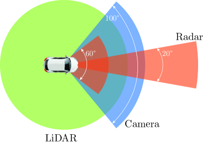
(a)

(b)

Figure 8: Vehicle configuration and sensor field-of-view (FOV). LiDAR FOV is shown in green, the camera FOV in blue and the radar FOV in orange.

We ran the Baidu’s Apollo AV stack on a computer with an Intel i9-9820X ($4.1\text{\,}\mathrm{GHz}$) processor, $64\text{\,}\mathrm{GB}$ of memory and two NVIDIA GeForce RTX 2080Ti. The simulator ran on a computer with 11th Generation Intel i7-11700F ($4.8\text{\,}\mathrm{GHz}$) processor, $16\text{\,}\mathrm{GB}$ of memory, and an NVIDIA GeForce RTX 3060. The two computers were connected using a Gigabit Ethernet cable.

7.2 Diagnostic Graph

We focused our attention on the obstacle detection pipeline. The system we aim to monitor, together with the failure modes considered, is shown in Fig. 9 The system is composed of four modules:

• Lidar-based Obstacle detector, based on a deep learning algorithm, subject to out-of-distribution sample failure mode;

• Camera-based Obstacle detector, based on a deep learning algorithm, subject to out-of-distribution sample failure mode;

• Radar-based Obstacle detector subject to misdetection failure mode;

• Sensor Fusion subject to misassociation failure mode.

Each module produces a set of detected obstacles. We identified three failure modes for each set of detected obstacles:

• misdetection: the module detected a ghost obstacle or is missing an obstacle in the scene;

• misposition: the module detected the obstacle correctly, but its position is incorrect (i.e., more than 2.5m error in our tests);

• misclassification: the module detected the obstacle correctly but the obstacle’s semantic class is incorrect.

We equipped the obstacle detection system with 18 diagnostic tests. For each pair of modules’ outputs, namely (Lidar, Camera), (Radar, Camera), (Lidar, Sensor Fusion), (Radar, Sensor Fusion), (Lidar, Radar), and (Camera, Sensor Fusion), there is a test that compares the outputs to diagnose each of the output’s failure modes (i.e., misdetection, misposition, and misclassification). Intuitively, each test compares the two sets of obstacles coming from the corresponding modules, and if they are different, it reports if the inconsistency was due to a misdetection, misposition, or misclassification. Moreover, we included a priori relation between every module and its output. In particular, the modules are assumed to fail if their outputs have at least one active failure mode. In the probabilistic diagnostic graph we also added an a priori relation for each module’s failure mode, indicating the prior probability of that failure mode being active.

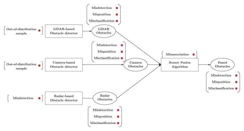
Figure 9: Perception system considered in our experiments. Modules are shown as rectangular blocks, outputs are shown as rounded boxes, while failure modes are denoted with red dots.

7.2.1 Diagnostic Tests

We now describe the logic for the diagnostic tests we implemented. Consider two sets of synchronized detected obstacles, say ${\cal A}$ and ${\cal B}$, produced by two modules, using some sensor data. Let $\Omega$ be the region defined by the intersection of both sensor fields of view and a region of interest (e.g., a region close to a drivable area). Denote by ${\cal A}_{\Omega}$ and ${\cal B}_{\Omega}$ the set of obstacles restricted to the region $\Omega$, namely ${\cal A}_{\Omega}\subseteq{\cal A}$ such that for each obstacle $o$ in ${\cal A}$, $o$ is in ${\cal A}_{\Omega}$ if and only if $o$ is inside the region defined by $\Omega$. The same relation holds for ${\cal B}_{\Omega}$. Then the diagnostic test checking for misdetections is defined as follows:

$$t_{\mathrm{misdetection}}=\begin{cases}\mathrm{FAIL}&\quad\mathrm{if}\left|{\cal A}_{\Omega}\right|\neq\left|{\cal B}_{\Omega}\right|\\ \mathrm{PASS}&\quad\mathrm{otherwise}\\ \end{cases}$$

Note that if the two sets of obstacles have a different cardinality —when restricted to the area co-visible by both sensors— it means that one of the two sets contains a ghost obstacle or one of the two sets is missing an obstacle. From a single test, we are not able to say which of the two sets is experiencing the misdetection, but we know at least one output did.

Let us now move our attention to the misposition failure mode. Let ${\cal C}$ be the set of matched obstacles, that is, a pair of obstacles $(l,r)$ —with $l\in{\cal A}_{\Omega}$ and $r\in{\cal B}_{\Omega}$— is in ${\cal C}$, if $l$ and $r$ represent the same obstacles. A common approach for finding the set of matches is to select all the pairs that are closest to each other (i.e., solving an assignment problem). The diagnostic test checking for mispositioned obstacles is defined as follows:

$$t_{\mathrm{misposition}}=\begin{cases}\mathrm{FAIL}&\quad\exists(l,r)\in{\cal C}\mbox{ such that }|\mathop{pos}\nolimits(l)-\mathop{pos}\nolimits(r)|\geq\theta\\ \mathrm{PASS}&\quad\mathrm{otherwise}\\ \end{cases}$$

where $\mathop{pos}\nolimits({\cdot})$ is the position of an obstacle and $\theta$ is an error threshold, chosen as $\theta=$2.5\text{\,}\mathrm{m}$$ in our experiments.

Finally, the test checking for misclassified obstacles is defined as follows:

$$t_{\mathrm{misclassification}}=\begin{cases}\mathrm{FAIL}&\quad\exists(l,r)\in{\cal C}\text{ such that }\operatorname{cls}(l)\neq\operatorname{cls}(r)\\ \mathrm{PASS}&\quad\mathrm{otherwise}\\ \end{cases}$$

where $\operatorname{cls}({\cdot})$ is the class of the obstacle, i.e., the test fails if associated obstacles are assigned different semantic classes.

7.2.2 Temporal Diagnostic Graph

To build a temporal diagnostic graph we stack $2$ regular diagnostic graphs into a temporal diagnostic graph. In the probabilistic case, each module failure mode is connected to its successive (in time) via a priori relationships, which represent the transition probability between states in consecutive time steps. No temporal a priori relations are added in the deterministic case. We also added temporal tests. The logic of the tests presented in Section 7.2 is applicable to temporal tests with small changes. In temporal tests, the sets ${\cal A}$ and ${\cal B}$ are not time-synchronized anymore (e.g., they are obstacles detected by the same sensor at consecutive time stamps), therefore the position of each obstacle in each set must be adjusted for the distance the obstacle traveled between consecutive detections. To use the tests described earlier in the temporal domain we used the following approach. If the obstacle is equipped with an estimated velocity vector, since the time difference between detections is usually below $30\text{\,}\mathrm{ms}$, we assume constant speed and integrate the speed over the time interval to find an approximate position of each obstacle. When the velocity is not available, we use the average speed of an obstacle (for a given obstacle’s class) and adapt the misposition threshold $\theta$ to account for the uncertainty.

7.3 Fault Identification: Implementation Details

Deterministic Fault Identification. For the tests with the deterministic model, we assumed the Weaker-OR model for the diagnostic tests as described in Eq. 3. We used this model for both the regular diagnostic graph and the temporal diagnostic graph, and solved the optimization problem in Eq. 8 using Google OR-Tools [101] Integer Programming Solver.

Probabilistic Fault Identification. To perform probabilistic inference on the diagnostic graph, we transformed it into a factor graph and trained the potentials for each relation using the maximum margin learning algorithm described in Section 5.2 on the training dataset. We used the Hamming distance defined in Eq. 20 as the loss function ${\cal L}$. We set the regularization parameter to $\lambda=10$; see [85]. For each diagnostic graph, we perform inference using the max-product algorithm for a fixed number of iteration ($100$ iterations). In our implementation, we use the Grante library [102] to perform learning and inference over the factor graph.

Graph-Neural-Network-based Fault Identification. In Section 5.3 we saw that a graph neural network requires a feature for each node in the graph to perform neural message passing. We now discuss how we set the feature vector for each node in the graph. Recall that the GNN uses a pairwise undirected graph, where a node is either a failure mode or a test outcome. The feature ${\bm{x}}_{t_{k}}\in{{\mathbb{R}}^{2}}$ for a test $t_{k}$ is set as the one-hot encoding of the test outcome (i.e., $[1\;0]$ if the test passed, $[0\;1]$ if it failed). For the failure mode nodes we do not have any measurable quantity at runtime; we therefore use the training dataset to compute the feature vectors. In particular the feature vector ${\bm{x}}_{f_{i}}\in{{\mathbb{R}}^{2}}$ for a failure mode $f_{i}$ is computed as follow: let $\rho_{i}$ be the empirical probability that $f_{i}$ is ACTIVE, i.e., $\rho_{i}=\frac{1}{|{\cal W}|}\sum_{({\bm{z}},{\bm{f}})\in{\cal W}}\operatorname{\mathds{1}}[f_{i}=\mathrm{ACTIVE}]$; then the feature vector is chosen as ${\bm{x}}_{f_{i}}=[1-\rho_{i},\rho_{i}]^{^{\mathsf{T}}}$. Intuitively, the feature describes the prior probability of the failure mode $f_{i}$’s state.

We now discuss the architecture of the GNN. Our GNN is composed by a linear layer that embeds the feature vectors in ${{\mathbb{R}}^{16}}$, followed by a ReLU function. The output is then passed to a stack of graph convolution layers interleaved with ReLU activation functions. We tested four different graph convolution layers

• in the case of GCN, we stack $3$ layers with $16$ hidden channels each;

• in the case of GCNII, we stack $64$ layers with $16$ hidden channels each with $\alpha=0.1$, $\beta=0.4$;

• in the case of GIN, we stack $3$ layers with $16$ hidden channels each with the function $\zeta^{(k)}({\cdot})$ (cf. Eq. 19) being a 2-layer perceptron for $k=1,\ldots,3$;

• in the case of GraphSAGE, we stack $3$ (and $6$ for temporal diagnostic graphs) layers with mean aggregator and $16$ hidden channels each.

Finally, the readout function that converts the graph embedding to node labels is a linear layers followed by a softmax pooling. We perform an ablation of the different GNN architectures in Section 7.5.

We implemented the GNNs in PyTorch [93] and trained them on the training dataset for $100$ epochs using the Adam optimizer. To reduce the amount of guesswork in choosing an initial learning rate, we used the learning rate finder available in the PyTorch Lightning library [103]. The procedure is based on [104]: the learning rate finder does a small training run where the learning rate is increased after each processed batch and the corresponding loss is logged. Then, the learning rate is chosen to be the point with the steepest negative gradient.

Baselines. We compared the proposed monitors against two simple baselines. In the first baseline (label: “Baseline”), whenever a diagnostic test returns FAIL, all failure modes in its scope are considered active. In the second baseline (label: “Baseline (w/rel. scores)”), modules are ordered by a reliability score defined by the system designer. In our experiments we considered the radar to be more reliable than the sensor fusion, which is more reliable than the LiDAR, which in turn is more reliable than the camera. When a diagnostic test fails, this second baseline labels all the failure modes in the test scope associated to the least reliable module (and its outputs) as ACTIVE. For example if a diagnostic test comparing camera and LiDAR obstacles returns FAIL, the failure modes associated with the camera are the ones that are labeled active because the camera is considered less reliable than the LiDAR. Both baselines label a module’ failure modes as active if at least one of the module’s outputs is failing.

7.4 Scenarios

We designed a set of challenging scenarios to stress-test the Apollo Auto perception system. These scenarios were created using the LGSVL Simulator Visual Scenario Editor, which allows the user to create scenarios using a drag-and-drop interface. The vehicle behavior is tested on each scenario in a multitude of situations including different time of day (noon, 6 PM, 9 PM) or weather condition (rain and fog). The scenarios are described in LABEL:tab:scenarios.

Table 1: Scenarios.   Fault-free.   Fault-detected.

Scene	Fault Detection Results
Hidden Pedestrian. A pedestrian, initially occluded by a track parked on the right-hand side of the street, steps in front of the ego vehicle.
Overturned Truck. The ego vehicle encounters an overturned truck occupying the lane it is driving in. The scenario recreates an accident occurred in Taiwan where a Tesla hit an overturned truck on a highway [105].
Stopped Vehicle. While driving, the car in front of the ego vehicle makes a lane change to avoid the stationary car that is in their lane. This leaves the ego vehicle with little to no time to react to the stationary car.
Cut Off Left. While driving in the right lane on a three-lane road, a vehicle from the left lane cuts the ego vehicle off.
Cut Off Right. While driving in the left lane on a two-lane road, a vehicle from the right lane cuts the ego vehicle off while turning into a parking lot.
School Bus Intersection. The ego vehicle drives through an intersection. A school bus crosses the intersection coming from the left-hand side. As the ego vehicle crosses the intersection, a pedestrian steps into the intersection from the left-hand side.
Car in Front. A car is still in front of the ego vehicle preventing it to move forward.
Cones in the Lane. The ego vehicle is driving on a lane partially delimited by traffic cones, while another vehicle is driving in the opposite lane. After passing traffic cones, another vehicle exits a parking lot and merges right in front of the ego vehicle.
Cyclist. The ego vehicle is stopped at an intersection and as it starts driving through the intersection, a cyclist enters the field of view from the left-hand side of the intersection and rides right in front of the ego vehicle.
Turkeys. While driving on a straight road, the ego vehicle must avoid a collision with two turkeys that suddenly walk in front of the ego vehicle.

7.4.1 Dataset generation

We executed the diagnostic tests described in Section 7.2 every $0.3$ seconds, and used the corresponding test outcomes to perform fault identification. Time synchronization of the modules’ output is achieved by pairing outputs that are closest in time to each other. Ground-truth labels for the outputs’ failure modes are generated using the ground-truth detections provided by the simulator. In particular, to generate the label for each failure mode of an output, we used the three diagnostic tests described in Section 7.2.1 comparing the set of obstacles to the ground-truth detections. For a module $m$ instead, since all modules have only one failure mode, the associated failure mode $f_{m}$ is labeled as ACTIVE if and only if any failure mode if its output is ACTIVE. We collected $1650$ regular diagnostic graphs, and split them into $1320$ ($80\%$) training samples, $165$ ($10\%$) testing samples, and $165$ validation samples. We also collected $1590$ temporal diagnostic graphs, and split them into $1272$ ($80\%$) training samples, $159$ ($10\%$) testing samples, and $159$ validation samples.

7.5 Fault Detection and Identification Results

We used three metrics to evaluate the performance for both the fault detection and identification problems:

Accuracy

is the percentage of correctly detected (resp. identified) failures over the total number of samples;

Precision

measures the percentage of correct identifications over the number of failures the fault identification system reported; a monitor achieves high precision if it has a low rate of false alarms;

Recall

measures the percentage of correct identifications over the number of failures the system experienced; a monitor has high recall if it is able to catch a large fraction of failures occurring in the perception system.

Algorithm	Regular			Temporal
	All	Outputs	Modules	All	Outputs	Modules
Factor Graph	93.30	96.72	83.03	93.60	96.88	83.74
Deterministic	91.06	93.69	83.18	89.26	92.33	80.06
Baseline (w/rel. scores)	92.39	94.65	85.61	90.18	92.69	82.67
Baseline	84.85	89.09	72.12	83.90	87.73	72.39
GCN	92.27	96.01	81.06	91.79	96.06	78.99
GCNII	87.61	93.94	68.64	92.60	96.01	82.36
GIN	91.89	96.06	79.39	93.21	96.47	83.44
GraphSage	92.84	96.46	81.97	92.71	96.42	81.60

Table 2: Fault identification accuracy. Best accuracy if highlighted in green, second-best is highlighted in yellow.

Figure 10: Precision/Recall for regular diagnostic graphs. (Left) Modules, (Right) Outputs.

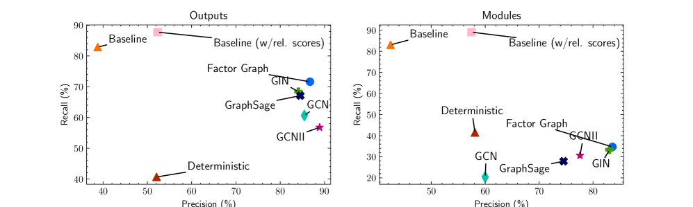
Figure 11: Precision/Recall for temporal diagnostic graphs. (Left) Modules, (Right) Outputs.

7.5.1 Fault Identification Results

Table 2 reports the accuracy of all compared techniques, averaged across all test scenarios in LABEL:tab:scenarios. The first and fourth columns report the overall accuracy (“All”) when using regular and temporal diagnostic graphs, respectively. The remaining columns report a breakdown of the accuracy in terms of modules and outputs. The overall accuracy results suggest that factor-graph-based probabilistic fault identification outperforms all other algorithms and achieves $96.72\text{\,}\mathrm{\char 37\relax}$ accuracy when using regular diagnostic graphs and $96.88\text{\,}\mathrm{\char 37\relax}$ with temporal diagnostic graphs. GNNs architectures achieve the second-best performance (GraphSAGE in the regular case, GIN in the temporal case). If we now look at the breakdown of the fault identification results between modules and outputs, we notice two trends. First, the factor graph still performs the best across the spectrum, but it is slightly slightly inferior than a baseline in the regular case. As we will see shortly, the baselines tend to make quite conservative decisions (i.e., they tend to detect more failures than the ones actually present in the system), which increases accuracy (and recall) at the expense of precision. Second, output fault identification has higher accuracy than module fault identification; this is expected, since most of our tests directly involve outputs, while we can only indirectly infer module failures via the a priori relations. Note that the two statistics (output fault identification vs. module fault identification) are typically used for different purposes, as discussed in Remark 2.

Fig. 10 shows precision-recall trade-offs when using regular diagnostic graphs. Best results are near the top-right corner of each figure, where both precision and recall are high. The figure confirms that while the baselines have large recall (due to the fact that are conservative in detecting failure modes as active), their precision is relatively low (i.e., they have a large number of false alarms). On the other side of the spectrum, GNN architectures (with the exception of GCNII) achieve high prediction ($87.25\text{\,}\mathrm{\char 37\relax}$ for GraphSAGE) but low recall ($60.96\text{\,}\mathrm{\char 37\relax}$ for GraphSAGE). The deterministic fault identification struggles to mark failure modes as active, achieving low precision and recall in the output space; this is due to the fact that it disregards PASS results (which do not even appear in the optimization Eq. 8). Factor graph inference again achieves a reasonable trade-off, with $85.22\text{\,}\mathrm{\char 37\relax}$ precision and $67.12\text{\,}\mathrm{\char 37\relax}$ recall.

Fig. 11 shows precision-recall trade-offs when using temporal diagnostic graphs. Compared to the regular diagnostic graph we see a steep increase in precision in the output space. The best-performing model goes from around $90\text{\,}\mathrm{\char 37\relax}$ precision of the regular graph to $97\text{\,}\mathrm{\char 37\relax}$ of the temporal diagnostic graph.

PAC-Diagnosability. Fig. 12 and Fig. 13 show the PAC-Diagnosability bound defined in Eq. 23 for each of the compared techniques. The bound represents the number of fault identification mistakes each algorithm is expected to make with a given confidence ($\delta$ in Eq. 23). The plots show that with high probability, most of the algorithms are expected to make less than $1$ mistake in the fault identification (i.e., false alarms or false negatives). The factor graph has the lowest bound of all methods in both the regular and temporal diagnostic graphs; the only exception is Fig. 12(right), where the baseline with reliability score has the lowest bound for module fault identification.

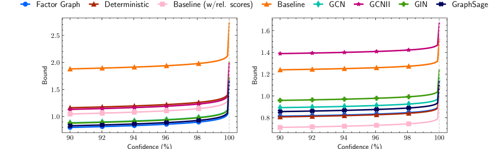
Figure 12: PAC-diagnosability bounds for regular diagnostic graphs. (Left) Modules, (Right) Outputs. Lower is better.

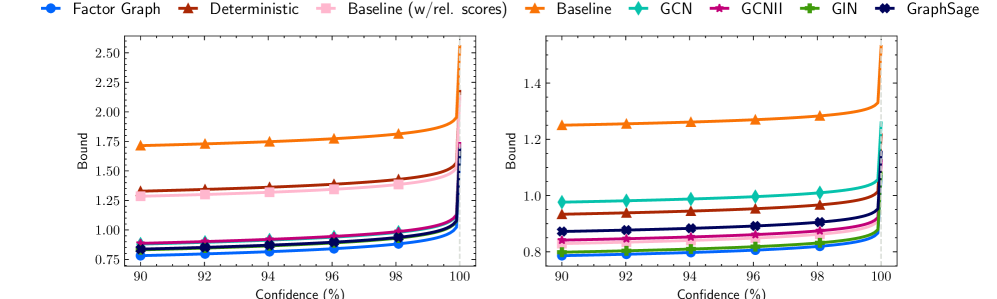
Figure 13: PAC-diagnosability bounds for temporal diagnostic graphs. (Left) Modules, (Right) Outputs. Lower is better.

$\kappa$-diagnosability. Let us now discuss the deterministic diagnosability of the perception system considered in our experiments (Fig. 9). If the tests behave as a Deterministic OR, the diagnostic graph used in our experiments is $5$-diagnosable. This means that if there are up to $5$ active failure modes the deterministic fault identification will be able to correctly identify them. If we instead assume the tests behave as a Weak-OR, which might fail when all the failure modes in its scope are active, the diagnostic graph is $3$-diagnosable. It’s worth noticing that this does not mean that if there are more than $3$ (or $5$) active failure modes the fault identification will surely fail, but rather that we do not have the guarantee that it will not make any mistake. When using Deterministic Weaker-OR tests, the diagnosability drops to zero, meaning that the fault identification guarantees vanish.

Extra diagnosability results. To show the effectiveness of the deterministic and probabilistic diagnosability we generated a random $4$-diagnosable diagnostic graph with $10$ independent failure modes and Weak-OR tests and collected the fault identification results (using the deterministic model) for every syndrome and every possible fault assignment. The results are shown in Fig. 14. The figure reports the average number of incorrect fault identification results (i.e., the Hamming distance between the estimated and actual vector of active faults) for increasing number of active faults. The vertical dashed line represents the deterministic diagnosability value: by Definition 16, the fault identification is guaranteed to correctly identify the active failure modes provided that there are less than $4$ active failure modes. In fact, from the plot we see that the fault identification algorithm does not make any mistake in the fault identification when there are less than $4$ faults. The horizontal dashed line instead represents the probabilistic diagnosability value, in particular it is the ceiling of the bound in Eq. 23, computed with very high confidence ($1\!-\!1\!\times\!10^{-12}$). The bound guarantees that with high probability the average number of mistakes (the average Hamming distance) the fault identification algorithm is going to make is less that $2$; this is again consistent with the numerical results.

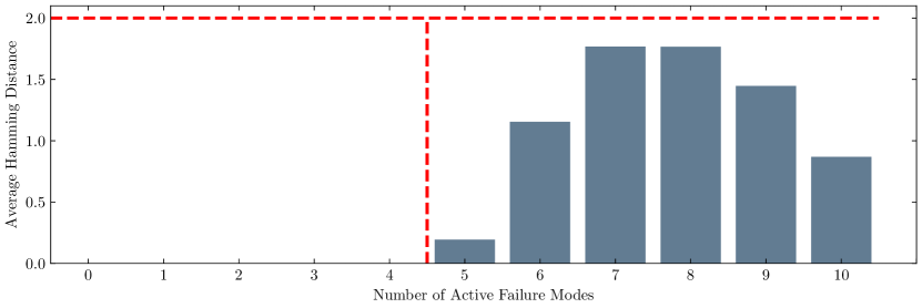
Figure 14: Average Hamming distance between the estimated and actual vector ${\bm{f}}$ of fault states in a randomly generated $4$-diagnosable diagnostic graph with $10$ independent failure modes and Weak-OR tests. The vertical dashed line represents the deterministic diagnosability bound: if the system is experiencing less than $4$ active failure modes, the fault identification is guaranteed to be correct ($0$ Hamming distance). The horizontal dashed line represents the ceiling of the PAC-diagnosability bound in Eq. 23: with very high probability the average number of mistakes (average Hamming distance) is less than the PAC-diagnosability bound.

Timing. The runtime of each method is shown in Table 3. All algorithms perform inference in less than $4\text{\,}\mathrm{ms}$, except for GCNII which averages at around $20\text{\,}\mathrm{ms}$. This is likely due to the fact that GCNII uses a deep architecture, which incurs an increased computational cost. The best performing algorithm, i.e., the factor graph, can be executed in real-time as its runtime averages around $0.8\text{\,}\mathrm{ms}$ for regular graphs and $3.8\text{\,}\mathrm{ms}$ for temporal graphs.

		Factor Graph	Deterministic	Baseline (w/rel. scores)	Baseline	GCN	GCNII	GIN	GraphSage
Regular	Avg.	0.79	3.25	0.10	0.10	0.63	19.88	0.48	0.59
	Std.	(0.17)	(0.14)	(0.06)	(0.06)	(0.01)	(0.10)	(0.01)	(0.02)
Temporal	Avg.	2.53	3.68	0.27	0.26	0.68	24.56	0.50	0.85
	Std.	(0.04)	(0.46)	(0.17)	(0.16)	(0.01)	(0.33)	(0.01)	(0.01)

Table 3: Average runtime (“Avg.”) and standard deviation (“Std.”) for fault identification, in milliseconds.

7.5.2 Fault Detection Results

Recall that fault detection is the problem of deciding whether the system is working in normal conditions or whether at least a fault has occurred. Table 4 and Fig. 15 show accuracy, precision, and recall. Fig. 15 shows that most of the algorithms for inference presented in this paper (as well as the baselines) attain similar performance with precision above $90\text{\,}\mathrm{\char 37\relax}$ and recall above $80\text{\,}\mathrm{\char 37\relax}$; this confirms that fault detection is a somewhat easier problem compared to fault identification. Table 4 shows that the deterministic approach and the baselines do particularly well for fault detection: they both detect failure as soon as a single test fails, which makes their accuracy high. On the other hand, the factor graph approach may prefer explaining a failed test as a false alarm. Therefore, while factor graphs would be the go-to approach for fault identification, a simpler baseline approach suffices for fault detection.

Algorithm	Regular			Temporal
	All	Outputs	Modules	All	Outputs	Modules
Factor Graph	76.67	88.48	64.85	81.60	91.41	71.78
Deterministic	89.09	89.09	89.09	93.25	93.25	93.25
Baseline (w/rel. scores)	89.09	89.09	89.09	85.28	85.28	85.28
Baseline	89.09	89.09	89.09	85.28	85.28	85.28
GCN	71.82	86.06	57.58	80.06	90.18	69.94
GCNII	68.48	87.88	49.09	78.83	85.89	71.78
GIN	83.94	86.06	81.82	83.13	92.64	73.62
GraphSage	76.67	89.09	64.24	79.14	89.57	68.71

Table 4: Fault detection accuracy. Best accuracy if highlighted in green, second-best is highlighted in yellow.

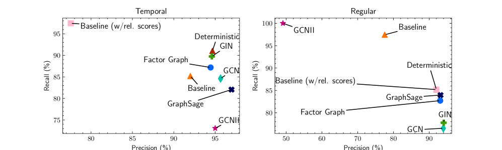
Figure 15: Fault detection in diagnostic graphs. (Left) Regular, (Right) Temporal.

7.6 Example Scenario: Using Monitoring to Prevent Accidents

We conclude the experimental section by showing how fault detection and identification can be effectively used to prevent dangerous situations. To this aim, we developed an additional scenario (not included in LABEL:tab:scenarios) where a deer crosses the road while the ego vehicle cruises on a straight road (Fig. 16).

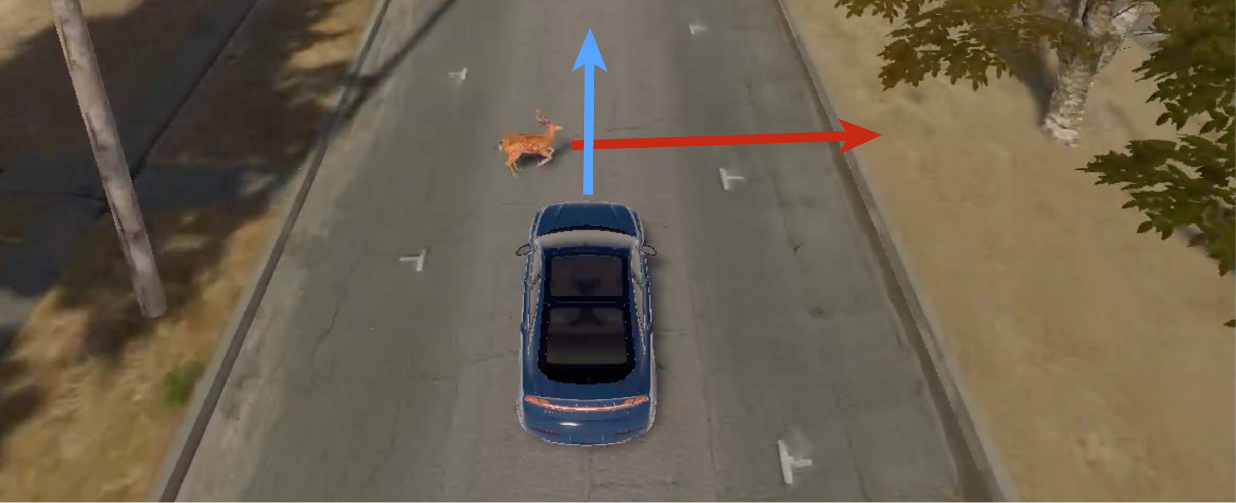
Figure 16: Example scenario involving a deer crossing the road in front of the ego vehicle.

The scenario is novel to the identification algorithm, i.e., not used for training, test, or validation. The results of the failure identification are shown in Fig. 17, where we used the probabilistic fault identification.

Figure 17: Fault identification results for the example scenario in Fig. 16. The car travels from right to left. Initially, the monitor detects no failure (rightmost, green section). As the ego vehicle gets closer to the obstacle, the LiDAR-based and camera-based obstacle detectors fail to detect the deer while the radar-based obstacle detector correctly locates the obstacle; as a result the fault identification/detection triggers an alarm (red sections).

Initially, the monitor detects no failure (rightmost green section). As the ego vehicle gets closer to the undetected obstacle, the radar detects the obstacle but the camera does not. The inconsistency between the two sets of obstacles causes the test between camera and radar to return FAIL. Given the test’s outcomes, the factor graph correctly detects and identifies the failure, triggering an alarm (rightmost red section). As the ego vehicle gets even closer, the deer goes out of the field-of-view of the radar while entering the LiDAR field-of-view. For a few meters, both camera and LiDAR fail to detect the deer Fig. 18, but since it is out of the field-of-view of the radar, the diagnostic test fails to report the failure. As the obstacle re-enters the field-of-view of the radar, the diagnostic test again returns FAIL, signaling the presence of a failure.

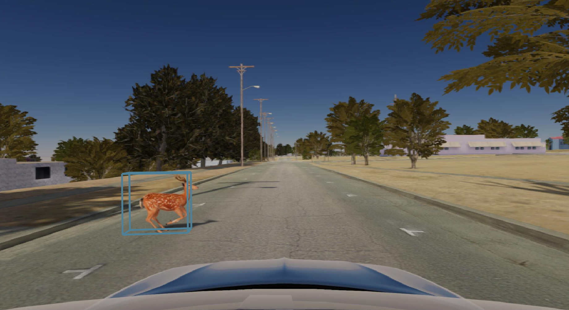
Figure 18: Camera Image for the scenario in Fig. 16. Blue bounding box is the ground truth detection. The camera fails to detect the deer crossing the road (misdetection failure).

The first alarm is raised $7.19\text{\,}\mathrm{s}$ before the collision, flagging the camera misdetection as an active failure mode. Before the collision, the AV has a speed of $8.43\text{\,}\mathrm{m}\mathrm{/}\mathrm{s}$. The car can reach a maximum deceleration of $6\text{\,}\mathrm{m}\text{\,}{\mathrm{s}}^{-2}$. As result, the car would need $1.4\text{\,}\mathrm{s}$ to come to a complete stop. We note that after detecting the fault, for a short interval of time the monitor detects no failure: this is due to the fact that the deer goes out of the radar field-of-view, and no other obstacle detector is capable of detecting it, thus lacking redundancy to diagnose the failure; see the visualization and explanation in Fig. 19.

To gather statistical evidence of the effectiveness of the fault detection, we run the same scenario 10 times at different times of the day (sun, twilight, and night) and different weather conditions (including fog and rain). The probabilistic fault detection approach never raised false alarms in these tests, and the average time between the alarm and the collision was $7.54\text{\,}\mathrm{s}$. The car traveled at an average speed of $6.16\text{\,}\mathrm{m}\mathrm{/}\mathrm{s}$, requiring $1.03\text{\,}\mathrm{s}$ to come to a complete stop. The fault identification exhibited an average accuracy of $93.75\text{\,}\mathrm{\char 37\relax}$.

(a)

(b)

Figure 19: Two snapshots from the example scenario of Fig. 16. Shaded areas represent the sensor field-of-view (FOV): green, blue, and orange represent the LiDAR, camera, and radar FOVs, respectively. On the left, the deer is outside the LiDAR FOV (so the LiDAR obstacle detector is not supposed to detect the obstacle); the radar detects the obstacle, while the camera fails to detect it even if it is inside its FOV. Since the corresponding diagnostic test fails, our monitors can detect the failure. On the right, the deer is outside the radar FOV; in this case, both the camera and the LiDAR fail to detect the obstacles (even though it is within their FOVs), hence no diagnostic test fails and our monitor fails to detect the fault.

8 Conclusions

This paper investigated runtime monitoring of complex perception systems and presented a novel framework to collect and organize diagnostic information for fault detection and identification in perception systems. Toward this goal, we formalized the concept of diagnostic tests, a generalization of runtime monitors, that return diagnostic information about the presence of failure modes. We then introduced the concept of diagnostic graph, as a structure to organize diagnostic information and its relations with the monitored perception system. We then provided a set of deterministic, probabilistic, and learning-based algorithms that use diagnostic graphs to perform fault detection and identification. In addition to the algorithms, we investigated fundamental limits and provided deterministic and probabilistic guarantees on the fault detection and identification results. These include results about the maximum number of faults that can be correctly identified in a given perception system as well as PAC-bounds on the number of mistakes our fault identification algorithms are expected to make. We conclude the paper with an extensive experimental evaluation, which recreates several realistic failure modes in the LGSVL open-source autonomous driving simulator, and applies the proposed system monitors to a state-of-the-art autonomous driving software stack (Baidu’s Apollo Auto). The results show that the proposed system monitors outperform baselines in terms of fault identification accuracy, have the potential of preventing accidents in realistic scenarios, and incur a negligible computational overhead.

This work opens a number of avenues for future work. First, we plan to test our monitors on real-world datasets (rather than realistic simulations) and to provide more examples of the proposed approach applied to other perception subsystems (e.g., localization, lane segmentation). Second, we plan to add a risk metric to the fault identification process that could help the decision layer to make more informed decisions. Finally, in this paper, we used simple diagnostic tests. Moving forward, it would be desirable to use more advanced diagnostic tests available in the literature.

References

- [1] Google’s self-driving startup Waymo is introducing fully driverless rides to San Francisco, https://www.businessinsider.com/waymo-testing-fully-automated-cars-san-francisco-2022-3, accessed: 2022-05-14.
- [2] G. Silberg, R. Wallace, G. Matuszak, J. Plessers, C. Brower, D. Subramanian, Self-driving cars: The next revolution, White paper, KPMG LLP & Center of Automotive Research 9 (2) (2012) 132–146.
-
[3]
NTSB,
Collision
between vehicle controlled by developmental automated driving system and
pedestrian, tempe, arizona (2018).
URL https://www.ntsb.gov/investigations/AccidentReports/Reports/HAR1903.pdf - [4] American Automobile Association, Active driving assistance system performance, https://newsroom.aaa.com/asset/active-driving-assistance-system-performance-may-2022/ (2022).
- [5] Waymo and Cruise self-driving cars took over San Francisco streets at record levels in 2021 — so did collisions with other cars, scooters, and bikes, https://www.businessinsider.com/self-driving-car-accidents-waymo-cruise-tesla-zoox-san-francisco-2022-1, accessed: 2022-05-14.
- [6] H. Yang, J. Shi, L. Carlone, TEASER: Fast and Certifiable Point Cloud Registration, arXiv preprint arXiv: 2001.07715(pdf).
- [7] M. Fischler, R. Bolles, Random sample consensus: a paradigm for model fitting with application to image analysis and automated cartography, Commun. ACM 24 (1981) 381–395.
- [8] R. Salay, R. Queiroz, K. Czarnecki, An analysis of iso 26262: Using machine learning safely in automotive software, arXiv preprint arXiv:1709.02435.
- [9] ISO Standard, Road vehicles — safety of the intended functionality, iSO/PAS 21448:2019(en) (2019).
-
[10]
Aptiv, Audi, B. Apollo, BMW, Continental, Daimler, F. Group, Here, Infineon,
Intel, Volkswagen,
Safety
First for Automated Driving (2019).
URL https://www.daimler.com/innovation/case/autonomous/safety-first-for-automated-driving-2.html - [11] H. Jing, Y. Gao, S. Shahbeigi, M. Dianati, Integrity monitoring of gnss/ins based positioning systems for autonomous vehicles: State-of-the-art and open challenges, IEEE Transactions on Intelligent Transportation Systems.
- [12] O. A. Hafez, G. D. Arana, M. Joerger, M. Spenko, Quantifying robot localization safety: A new integrity monitoring method for fixed-lag smoothing, IEEE Robotics and Automation Letters 5 (2) (2020) 3182–3189.
- [13] V. Besnier, A. Bursuc, D. Picard, A. Briot, Triggering failures: Out-of-distribution detection by learning from local adversarial attacks in semantic segmentation, in: Proceedings of the IEEE/CVF International Conference on Computer Vision, 2021, pp. 15701–15710.
- [14] F. P. Preparata, G. Metze, R. T. Chien, On the connection assignment problem of diagnosable systems, IEEE Transactions on Electronic Computers (6) (1967) 848–854.
-
[15]
LG, LGSVL Simulator.
URL https://www.lgsvlsimulator.com -
[16]
Baidu, Apollo Auto.
URL https://apollo.auto/ - [17] S. Shalev-Shwartz, S. Shammah, A. Shashua, On a formal model of safe and scalable self-driving cars, ArXiv abs/1708.06374.
- [18] N. Kalra, S. M. Paddock, Driving to safety: How many miles of driving would it take to demonstrate autonomous vehicle reliability?, Transportation Research Part A: Policy and Practice 94 (2016) 182–193.
- [19] ISO Standard, Road vehicles – functional safety, iSO 26262-1:2011 (2011).
- [20] P. Koopman, M. Wagner, Challenges in autonomous vehicle testing and validation, SAE Int. J. Trans. Safety 4 (1).
- [21] F. Concas, J. K. Nurminen, T. Mikkonen, S. Tarkoma, Validation Frameworks for Self-Driving Vehicles: A Survey, Springer, 2021.
- [22] P. Koopman, U. Ferrell, F. Fratrik, M. Wagner, A safety standard approach for fully autonomous vehicles, in: International Conference on Computer Safety, Reliability, and Security, Springer, 2019, pp. 326–332.
-
[23]
Underwriters Laboratories, ANSI/UL 4600
Standard for Safety for the Evaluation of Autonomous Products.
URL https://ul.org/UL4600 - [24] F. Ingrand, Recent trends in formal validation and verification of autonomous robots software, in: 2019 Third IEEE International Conference on Robotic Computing (IRC), 2019, pp. 321–328.
- [25] A. Desai, T. Dreossi, S. Seshia, Combining model checking and runtime verification for safe robotics, in: International Conference on Runtime Verification, Springer, 2017, pp. 172–189.
- [26] B. Hoxha, G. Fainekos, Planning in dynamic environments through temporal logic monitoring, in: AAAI Workshop: Planning for Hybrid Systems, Vol. 16, 2016, p. 12.
- [27] C.-I. Vasile, J. Tumova, S. Karaman, C. Belta, D. Rus, Minimum-violation scLTL motion planning for mobility-on-demand, in: IEEE Intl. Conf. on Robotics and Automation (ICRA), 2017, pp. 1481–1488.
- [28] S. Dathathri, R. Murray, Decomposing GR(1) games with singleton liveness guarantees for efficient synthesis, arXiv abs/1709.07094.
- [29] S. Ghosh, D. Sadigh, P. Nuzzo, V. Raman, A. Donzé, A. L. Sangiovanni-Vincentelli, S. S. Sastry, S. A. Seshia, Diagnosis and repair for synthesis from signal temporal logic specifications, in: Proceedings of the 19th International Conference on Hybrid Systems: Computation and Control, HSCC ’16, ACM, 2016, pp. 31–40.
- [30] W. Li, L. Dworkin, S. A. Seshia, Mining assumptions for synthesis, in: Ninth ACM/IEEE International Conference on Formal Methods and Models for Codesign (MEMPCODE2011), 2011, pp. 43–50.
- [31] W. Li, D. Sadigh, S. Sastry, S. Seshia, Synthesis for human-in-the-loop control systems, in: Intl. Conf. on Tools and Algorithms for the Construction and Analysis of Systems (TACAS), 2014.
- [32] M. Kloetzer, C. Belta, A fully automated framework for control of linear systems from temporal logic specifications, IEEE Trans. on Automatic Control 53 (1) (2008) 287–297.
- [33] S. Mitsch, K. Ghorbal, D. Vogelbacher, A. Platzer, Formal verification of obstacle avoidance and navigation of ground robots, The International Journal of Robotics Research 36 (12) (2017) 1312–1340.
- [34] N. Roohi, R. Kaur, J. Weimer, O. Sokolsky, I. Lee, Self-driving vehicle verification towards a benchmark, arXiv preprint arXiv:1806.08810.
- [35] R. C. Cardoso, M. Farrell, M. Luckcuck, A. Ferrando, M. Fisher, Heterogeneous verification of an autonomous curiosity rover (2020) 353–360.
- [36] S. Jha, V. Raman, D. Sadigh, S. Seshia, Safe autonomy under perception uncertainty using chance-constrained temporal logic, Journal of Automated Reasoning 60 (2017) 43–62.
- [37] F. Pasqualetti, F. Dörfler, F. Bullo, Attack detection and identification in cyber-physical systems, IEEE Transactions on Automatic Control 58 (11) (2013) 2715–2729.
- [38] M. Foughali, B. Berthomieu, S. Dal Zilio, P.-E. Hladik, F. Ingrand, A. Mallet, Formal verification of complex robotic systems on resource-constrained platforms, in: 2018 IEEE/ACM 6th International FME Workshop on Formal Methods in Software Engineering (FormaliSE), 2018, pp. 2–9.
- [39] S. Seshia, D. Sadigh, Towards verified artificial intelligence, ArXiv abs/1606.08514.
- [40] M. Luckcuck, M. Farrell, L. A. Dennis, C. Dixon, M. Fisher, Formal specification and verification of autonomous robotic systems: A survey, ACM Computing Surveys (CSUR) 52 (5) (2019) 1–41.
- [41] T. Dreossi, D. Fremont, S. Ghosh, E. Kim, H. Ravanbakhsh, M. Vazquez-Chanlatte, S. Seshia, VERIFAI: A toolkit for the design and analysis of artificial intelligence-based systems, ArXiv:1902.04245.
- [42] D. J. Fremont, T. Dreossi, S. Ghosh, X. Yue, A. L. Sangiovanni-Vincentelli, S. A. Seshia, Scenic: a language for scenario specification and scene generation, in: Proceedings of the 40th ACM SIGPLAN Conference on Programming Language Design and Implementation, 2019, pp. 63–78.
- [43] K. Leahy, E. Cristofalo, C. Vasile, A. Jones, E. Montijano, M. Schwager, C. Belta, Control in belief space with temporal logic specifications using vision-based localization, Intl. J. of Robotics Research 38.
- [44] A. Balakrishnan, A. G. Puranic, X. Qin, A. Dokhanchi, J. V. Deshmukh, H. Ben Amor, G. Fainekos, Specifying and evaluating quality metrics for vision-based perception systems, in: Design, Automation Test in Europe Conference Exhibition (DATE), 2019, pp. 1433–1438.
- [45] A. Dokhanchi, H. B. Amor, J. Deshmukh, G. Fainekos, Evaluating perception systems for autonomous vehicles using quality temporal logic, in: Intl. Conf. on Runtime Verification (RV), 2018.
- [46] T. Dreossi, S. Ghosh, A. Sangiovanni-Vincentelli, S. Seshia, Systematic testing of convolutional neural networks for autonomous driving, ArXiv abs/1708.03309.
- [47] Y. Cao, C. Xiao, B. Cyr, Y. Zhou, W. Park, S. Rampazzi, Q. A. Chen, K. Fu, Z. M. Mao, Adversarial sensor attack on lidar-based perception in autonomous driving, in: Proceedings of the 2019 ACM SIGSAC conference on computer and communications security, 2019, pp. 2267–2281.
- [48] A. Boloor, K. Garimella, X. He, C. Gill, Y. Vorobeychik, X. Zhang, Attacking vision-based perception in end-to-end autonomous driving models, Journal of Systems Architecture 110 (2020) 101766.
- [49] H. Delecki, M. Itkina, B. Lange, R. Senanayake, M. J. Kochenderfer, How do we fail? stress testing perception in autonomous vehicles, arXiv preprint arXiv:2203.14155.
- [50] N. Akhtar, A. Mian, Threat of adversarial attacks on deep learning in computer vision: A survey, Ieee Access 6 (2018) 14410–14430.
- [51] Q. M. Rahman, P. Corke, F. Dayoub, Run-time monitoring of machine learning for robotic perception: A survey of emerging trends, IEEE Access 9 (2021) 20067–20075.
- [52] D. Miller, P. Moghadam, M. Cox, M. Wildie, R. Jurdak, What’s in the black box? the false negative mechanisms inside object detectors, arXiv preprint arXiv:2203.07662.
- [53] Q. M. Rahman, N. Sünderhauf, P. Corke, F. Dayoub, Fsnet: A failure detection framework for semantic segmentation, Vol. 7, 2022, pp. 3030–3037. doi:10.1109/LRA.2022.3143219.
- [54] J. Lambert, J. Hays, Trust, but verify: Cross-modality fusion for hd map change detection, in: Thirty-fifth Conference on Neural Information Processing Systems Datasets and Benchmarks Track (Round 2), 2021.
- [55] J. Liu, J.-M. Park, “seeing is not always believing”: Detecting perception error attacks against autonomous vehicles, IEEE Transactions on Dependable and Secure Computing 18 (5) (2021) 2209–2223.
- [56] A. Sharma, N. Azizan, M. Pavone, Sketching curvature for efficient out-of-distribution detection for deep neural networks, in: Uncertainty in Artificial Intelligence, PMLR, 2021, pp. 1958–1967.
- [57] C. You, Z. Hau, S. Demetriou, Temporal consistency checks to detect lidar spoofing attacks on autonomous vehicle perception, in: Proceedings of the 1st Workshop on Security and Privacy for Mobile AI, 2021, pp. 13–18.
- [58] A. Balakrishnan, J. Deshmukh, B. Hoxha, T. Yamaguchi, G. Fainekos, Percemon: Online monitoring for perception systems, in: International Conference on Runtime Verification, Springer, 2021, pp. 297–308.
- [59] D. Kang, D. Raghavan, P. Bailis, M. Zaharia, Model assertions for debugging machine learning, in: NIPS, 2018.
- [60] A. Santamaria-Navarro, R. Thakker, D. D. Fan, B. Morrell, A. akbar Agha-mohammadi, Towards resilient autonomous navigation of drones (2020). arXiv:2008.09679.
- [61] B. Cai, L. Huang, M. Xie, Bayesian networks in fault diagnosis, IEEE Transactions on industrial informatics 13 (5) (2017) 2227–2240.
- [62] A. Abdollahi, K. R. Pattipati, A. Kodali, S. Singh, S. Zhang, P. B. Luh, Probabilistic graphical models for fault diagnosis in complex systems, in: Principles of Performance and Reliability Modeling and Evaluation, Springer, 2016, pp. 109–139.
- [63] Y. Lei, B. Yang, X. Jiang, F. Jia, N. Li, A. K. Nandi, Applications of machine learning to machine fault diagnosis: A review and roadmap, Mechanical Systems and Signal Processing 138 (2020) 106587.
- [64] X. Ma, J. Wu, S. Xue, J. Yang, C. Zhou, Q. Z. Sheng, H. Xiong, L. Akoglu, A comprehensive survey on graph anomaly detection with deep learning, IEEE Transactions on Knowledge and Data Engineering.
- [65] J. De Kleer, B. C. Williams, Diagnosing multiple faults, Artificial intelligence 32 (1) (1987) 97–130.
- [66] S. L. Hakimi, A. T. Amin, Characterization of connection assignment of diagnosable systems, IEEE Transactions on Computers 100 (1) (1974) 86–88.
- [67] K. Bhat, Algorithms for finding diagnosability level and t-diagnosis in a network of processors, in: Proceedings of the ACM’82 conference, 1982, pp. 164–168.
- [68] A. T. Dahbura, System-level diagnosis: A perspective for the third decade, in: Concurrent Computations, Springer, 1988, pp. 411–434.
- [69] M. Sampath, R. Sengupta, S. Lafortune, K. Sinnamohideen, D. Teneketzis, Diagnosability of discrete-event systems, IEEE Transactions on automatic control 40 (9) (1995) 1555–1575.
- [70] J. Zaytoon, S. Lafortune, Overview of fault diagnosis methods for discrete event systems, Annual Reviews in Control 37 (2) (2013) 308–320.
- [71] T. M. Tuxi, L. K. Carvalho, E. V. Nunes, A. E. da Cunha, Diagnosability verification using ltl model checking, Discrete Event Dynamic Systems (2022) 1–35.
- [72] P. Antonante, D. Spivak, L. Carlone, Monitoring and diagnosability of perception systems, in: IEEE/RSJ Intl. Conf. on Intelligent Robots and Systems (IROS), 2021, (pdf).
- [73] H. Yang, L. Carlone, Certifiable outlier-robust geometric perception: Exact semidefinite relaxations and scalable global optimization, arXiv preprint arXiv: 2109.03349(pdf).
- [74] J. Yang, M. Ward, J. Akhtar, The development of safety cases for an autonomous vehicle: A comparative study on different methods, Tech. rep., SAE Technical Paper (2017).
- [75] R. Yan, S. J. Dunnett, L. M. Jackson, Reliability modelling of automated guided vehicles by the use of failure modes effects and criticality analysis, and fault tree analysis, in: 5th student conference on operational research (SCOR 2016), Schloss Dagstuhl-Leibniz-Zentrum fuer Informatik, 2016.
- [76] P. Antonante, D. Spivak, L. Carlone, Monitoring and diagnosability of perception systems, arXiv preprint arXiv: 2011.07010(pdf).
-
[77]
H. Yang, L. Carlone,
One
ring to rule them all: Certifiably robust geometric perception with
outliers, in: Conference on Neural Information Processing Systems (NeurIPS),
Vol. 33, 2020, pp. 18846–18859,
(pdf).
URL https://proceedings.neurips.cc/paper/2020/file/da6ea77475918a3d83c7e49223d453cc-Paper.pdf - [78] H. Yang, L. Carlone, In perfect shape: Certifiably optimal 3D shape reconstruction from 2D landmarks, in: IEEE Conf. on Computer Vision and Pattern Recognition (CVPR), 2020, arxiv version: 1911.11924, (pdf).
- [79] H. Yang, L. Carlone, A polynomial-time solution for robust registration with extreme outlier rates, in: Robotics: Science and Systems (RSS), 2019, (pdf), (video), (media), (media), (media).
- [80] C. Cadena, L. Carlone, H. Carrillo, Y. Latif, D. Scaramuzza, J. Neira, I. Reid, J. Leonard, Past, present, and future of simultaneous localization and mapping: Toward the robust-perception age, IEEE Trans. Robotics 32 (6) (2016) 1309–1332, arxiv preprint: 1606.05830, (pdf). doi:10.1109/TRO.2016.2624754.
- [81] H. Yang, J. Shi, L. Carlone, TEASER: Fast and Certifiable Point Cloud Registration, IEEE Trans. Robotics 37 (2) (2020) 314–333, extended arXiv version 2001.07715 (pdf).
- [82] L. A. Wolsey, Integer programming, John Wiley & Sons, 2020.
- [83] F. Rossi, P. Van Beek, T. Walsh, Handbook of constraint programming, Elsevier, 2006.
- [84] S. E. Shimony, Finding maps for belief networks is np-hard, Artificial intelligence 68 (2) (1994) 399–410.
- [85] S. Nowozin, C. H. Lampert, Structured learning and prediction in computer vision, Vol. 6, Now publishers Inc, 2011.
- [86] K. P. Murphy, Machine learning: a probabilistic perspective, MIT press, 2012.
- [87] W. L. Hamilton, Graph representation learning, Synthesis Lectures on Artifical Intelligence and Machine Learning 14 (3) (2020) 1–159.
- [88] T. Kipf, M. Welling, Semi-supervised classification with graph convolutional networks, in: Intl. Conf. on Learning Representations (ICLR), 2017.
- [89] Q. Li, Z. Han, X.-M. Wu, Deeper insights into graph convolutional networks for semi-supervised learning, in: Thirty-Second AAAI conference on artificial intelligence, 2018.
- [90] M. Chen, Z. Wei, Z. Huang, B. Ding, Y. Li, Simple and deep graph convolutional networks, in: International Conference on Machine Learning, PMLR, 2020, pp. 1725–1735.
- [91] W. H. L., R. Ying, J. Leskovec, Inductive representation learning on large graphs, in: Advances in Neural Information Processing Systems (NIPS), 2017, p. 1025–1035.
- [92] K. Xu, W. Hu, J. Leskovec, S. Jegelka, How powerful are graph neural networks?, in: Intl. Conf. on Learning Representations (ICLR), 2019.
- [93] A. Paszke, S. Gross, F. Massa, A. Lerer, J. Bradbury, G. Chanan, T. Killeen, Z. Lin, N. Gimelshein, L. Antiga, et al., Pytorch: An imperative style, high-performance deep learning library, Advances in neural information processing systems 32.
- [94] A. Sengupta, A. T. Dahbura, On self-diagnosable multiprocessor systems: diagnosis by the comparison approach, IEEE Transactions on Computers 41 (11) (1992) 1386–1396.
-
[95]
Baidu, Apollo Auto.
URL https://github.com/ApolloAuto/apollo - [96] Z. Liu, Z. Wu, R. Tóth, SMOKE: Single-stage monocular 3d object detection via keypoint estimation, arXiv preprint arXiv:2002.10111.
- [97] P. Sun, H. Kretzschmar, X. Dotiwalla, A. Chouard, V. Patnaik, P. Tsui, J. Guo, Y. Zhou, Y. Chai, B. Caine, et al., Scalability in perception for autonomous driving: Waymo open dataset, in: Proceedings of the IEEE/CVF Conference on Computer Vision and Pattern Recognition, 2020, pp. 2446–2454.
- [98] A. H. Lang, S. Vora, H. Caesar, L. Zhou, J. Yang, O. Beijbom, Pointpillars: Fast encoders for object detection from point clouds, in: Proceedings of the IEEE/CVF Conference on Computer Vision and Pattern Recognition, 2019, pp. 12697–12705.
- [99] Google’s self-driving startup Waymo is introducing fully driverless rides to San Francisco, https://www.continental-automotive.com/getattachment/5430d956-1ed7-464b-afa3-cd9cdc98ad63/ARS408-21_datasheet_en_170707_V07.pdf.pdf, accessed: 2022-05-15.
- [100] D. F. Crouse, On implementing 2d rectangular assignment algorithms, IEEE Transactions on Aerospace and Electronic Systems 52 (4) (2016) 1679–1696.
-
[101]
Google, Google OR-Tools.
URL https://developers.google.com/optimization - [102] Grante Library for Inference and Estimation on Discrete Factor Graph Model, http://www.nowozin.net/sebastian/grante/, accessed: 2022-05-15.
- [103] W. Falcon, et al., Pytorch lightning, https://github.com/PytorchLightning/pytorch-lightning (2019).
- [104] L. N. Smith, Cyclical learning rates for training neural networks, in: 2017 IEEE winter conference on applications of computer vision (WACV), IEEE, 2017, pp. 464–472.
- [105] The Guardian, Tesla driver dies in first fatal crash while using autopilot mode, www.theguardian.com/technology/2016/jun/30/tesla-autopilot-death-self-driving-car-elon-musk, accessed: 2022-05-15 (2016).