On the classification of UV completions of integrable
$T\overline{T}$ deformations of CFT

Abstract

It is well understood that 2d conformal field theory (CFT) deformed by an irrelevant $T\overline{T}$ perturbation of dimension $4$ has universal properties. In particular, for the most interesting cases, the theory develops a singularity in the ultra-violet (UV), signifying a shortest possible distance, with a Hagedorn transition in applications to string theory. We show that by adding an infinite number of higher $[T\overline{T}]_{s>1}$ irrelevant operators of positive integer scaling dimension $2(s+1)$ with tuned couplings, this singularity can be resolved and the theory becomes UV complete with a Virasoro central charge $c_{{\rm UV}}>c_{{\rm IR}}$ consistent with the c-theorem. We propose an approach to classifying the possible UV completions of a given CFT perturbed by $[T\overline{T}]_{s}$ that are integrable. The main tool utilized is the thermodynamic Bethe ansatz. We study this classification for theories with scalar (diagonal) factorizable S-matrices. For the Ising model with $c_{{\rm IR}}=\tfrac{1}{2}$ we find 3 UV completions based on a single massless Majorana fermion description with $c_{{\rm UV}}=\tfrac{7}{10}$ and $\tfrac{3}{2}$, which both have ${\cal N}=1$ SUSY and were previously known, and we argue that these are the only solutions to our classification problem based on this spectrum of particles. We find 3 additional ones with a spectrum of 8 massless particles related to the Lie group $E_{8}$ appropriate to a magnetic perturbation with $c_{{\rm UV}}=\tfrac{21}{22},\tfrac{15}{2}$ and $\tfrac{31}{2}$. We argue that it is likely there are more cases for this $E_{8}$ spectrum. We also study simpler cases based on ${\rm su(3)}$ and ${\rm su(4)}$ where we can propose complete classifications. For ${\rm su(3)}$ the infrared (IR) theory is the 3-state Potts model with $c_{{\rm IR}}=\tfrac{4}{5}$ and we find 3 completions with $\tfrac{4}{5}<c_{{\rm UV}}\leq\tfrac{16}{5}$. For the ${\rm su(4)}$ case, which has $3$ particles and $c_{{\rm IR}}=1$, and we find $11$ UV completions with $1<c_{{\rm UV}}\leq 5$, most of which were previously unknown.

I Introduction

Suppose we are given a 2d conformal field theory (CFT), referred to as ${{\rm cft}_{{\rm IR}}}$, with Virasoro central charge $c\equiv c_{\rm IR}$, and we then consider irrelevant perturbations of this CFT:

$${\cal S}={\cal S}_{{{\rm cft}_{{\rm IR}}}}+\sum_{i\geq 1}\alpha_{i}\int d^{2}x\,{\cal O}_{i}(x),$$ (1)

where ${\cal O}_{i}$ are irrelevant operators of scaling dimension $\Gamma_{i}\geq 2$ in units of mass. Since the perturbing operators are irrelevant, the CFT describes the infrared (IR) fixed point of the above model, hence the label ${{\rm cft}_{{\rm IR}}}$. Here $\Gamma_{i}=2\Delta_{i}$ where $\Delta_{i}$ is the standard left/right conformal dimension. The couplings $\alpha_{i}$ have dimension $2-\Gamma_{i}$. We assume there is a single overall mass scale $M$, such that $\alpha_{i}\propto M^{2-\Gamma_{i}}$. There always exists an infinite number of possible irrelevant operators ${\cal O}_{i}$ in part because we can always differentiate lower dimension operators. The standard and essentially correct thinking is that starting with only a few non-zero $\alpha_{i}$, perturbation theory generates an infinite number of additional couplings $\alpha_{i}$, the ultraviolet (UV) limit does not exist, and predictability is lost. This article explores a fundamental question: can one tune the couplings $\alpha_{i}$ such that the UV limit exists? This general problem is fundamental to attempts to theorize beyond the Standard Model physics, since the central issue is to find a complete and finite UV theory, perhaps with quantum gravity, that leads to the low energy Standard Model under renormalization group (RG) flow. In quantum gravity, ultraviolet completeness is often referred to as “asymptotic safety” Weinberg . There are many interesting issues in connection with these questions. For instance, the c-theorem ctheorem indicates that RG flow to lower energies is “irreversible” in the sense that some UV degrees of freedom are lost in the flow. This leads to the basic question: “Can we reconstruct the UV theory from our limited data on the low energy infrared theory by somehow reversing the RG flow?”. In general the answer is obviously no, thus examples where it is possible, due perhaps to symmetries like supersymmetry, are intrinsically interesting. This is the problem studied in this paper in a specialized context. Theories of the kind studied here without a UV completion are in a sense analogous to the so-called “Swampland” Swampland .

The above question is very broadly stated, and in this paper we will limit its scope by imposing some significant additional structure. First we limit ourselves to integrable theories in $2$ spacetime dimensions. As we will see, this restriction still leads to a rich structure that has not been fully explored. There are in general an infinite number of low dimension irrelevant operators ${\cal O}_{i}$ to consider depending on the choice of ${{\rm cft}_{{\rm IR}}}$. However every CFT has a stress-energy tensor with the conventionally normalized left/right components $T(z)$ and $\overline{T}({\overline{z}})$, each of dimension $2$ in units of energy. We thus restrict the class of models such that the lowest dimension irrelevant operator is ${\cal O}_{1}=T\overline{T}/\pi^{2}$, and define $\alpha=\alpha_{1}$ of mass (energy) dimension $-2$. We thus define the dimensionless coupling $g=-\alpha M^{2}$. The higher dimensional operators $\{{\cal O}_{i>1}\}$ will be denoted $[T\overline{T}]_{s>1}$ with dimension $2(s+1)$ where $s$ is an odd integer, which will be based on the possible integrable perturbations of ${{\rm cft}_{{\rm IR}}}$ as described in SZ . More specifically, $s+1$ will be associated to the integer “spin” of a local conserved quantity where $T,\overline{T}$ in $[T\overline{T}]_{s}$ have spin $s+1$ and $-(s+1)$) respectively; this will be reviewed in the next section.

As already stated, for $s=1$, $[T\overline{T}]_{1}=T\overline{T}/\pi^{2}$ is associated to the generic energy-momentum conservation. If all other $\alpha_{s>1}=0$, then it is known that the ground state energy on a circle of circumference $R$ has a universal form SZ ; Tateo1 , which we now review. An important probe of any theory is the ground state energy $E(R)$ on an infinite cylinder of circumference $R$, which was studied in ZTT ; Tateo1 ; SZ . In thermodynamic language the free energy density is ${\cal F}(T)=E(R)/R$, where $R=1/T$ is the inverse temperature. It is standard to express this quantity in terms of a scaling function $c(MR)$

$$E(R)=-\dfrac{\pi}{6}\,\dfrac{c(MR)}{R}$$ (2)

where $M$ can be identified with a physical energy scale, such as the mass of a particle, or the energy scale of massless particles. The UV limit is $r\equiv MR\to 0$, whereas the IR corresponds to $r\to\infty$. For a conformal theory, $c(MR)$ is scale invariant, i.e. independent of $MR$, and for unitary theories is equal to the Virasoro central charge. For non-unitary theories it is shifted $c\to c-12d_{0}$ where $d_{0}$ is the lowest scaling dimension of fields. The quantity $c(MR)$ can be used to track the RG flow. It has been shown that

$$c(MR)=\dfrac{2c_{{\rm IR}}}{1+\sqrt{1-\dfrac{2\pi h}{3}c_{{\rm IR}}}},~{}~{}~{}~{}~{}h\equiv\dfrac{g}{(MR)^{2}}$$ (3)

where $c_{{\rm IR}}$ is a constant $-\infty<c_{{\rm IR}}<\infty$ identified as the IR central charge as $MR\to\infty$. This result was obtained in SZ ; Tateo1 based on the inviscid Burgers equation

$$\partial_{\alpha}E+E\partial_{R}E=0.$$ (4)

Indeed, one finds that (3) satisfies the above differential equation if one identifies

$$h=-\dfrac{\alpha}{R^{2}},~{}~{}~{}~{}~{}\Longrightarrow~{}~{}g=-\alpha\,M^{2}.$$ (5)

For $\alpha<0$ and $c_{{\rm IR}}>0$, one sees that the ground state energy develops a square-root singularity in the UV when $R^{2}<2\pi|\alpha|/3$, indicating a smallest possible distance. It is evident that this singularity only exists for negative $\alpha$ if $c_{{\rm IR}}>0$, and this is consistent with the c-theorem, i.e. $c(MR)$ increases toward the UV until the singularity is reached AL .

Depending on the context, the singularity in the UV may or may not be desirable. In the string context, the shortest possible distance is related to the string scale and thus a kind of Hagedorn transition, and there is no conceptual reason to try to add additional irrelevant operators Dubovsky ; Dubovsky2 ; Verlinde ; Cardy ; Tateo2 ; Tateo3 . On the other hand, in traditional QFT, the singularity signifies the usual pathology with irrelevant perturbations. In this paper we take the latter point of view, and try to cure the singularity.

To be more specific and summarize the models studied here, we consider a 2d CFT formally defined by the action:

$${\cal S}_{\alpha}={\cal S}_{{{\rm cft}_{{\rm IR}}}}+\sum_{s\geq 1}\alpha_{s}\,\int d^{2}x\,[T\overline{T}]_{s}$$ (6)

where the irrelevant operators $[T\overline{T}]_{s}$ depend on the ${{\rm cft}_{{\rm IR}}}$ and are defined in SZ , as reviewed in the next section. These generalized $T\overline{T}$ deformations have been considered recently in a somewhat different context Hernandez ; Doyon ; Camilo ; Cordova ; the main distinction from our work is that here the focus is on massless flows between CFT’s which was not studied in these works. The problem we pose and study is to classify the possible tuned $\alpha_{s}$ that have UV completions, i.e. theories that are non-singular in the UV. This means that in the UV the theories are relevant perturbations of a different CFT we denote as ${{\rm cft}_{{\rm UV}}}$ with central charge $c_{\rm UV}$:

$${\cal S}_{\rm UV}\approx{\cal S}_{{{\rm cft}_{{\rm UV}}}}+\lambda^{\prime}\int d^{2}x\,\Phi_{{\rm rel}}^{{\rm uv}}\,.$$ (7)

The parameters and characteristics of a UV complete model are $c_{\rm IR}$, $c_{\rm UV}$, the tuned parameters $\alpha_{s}$ and the dimension of the relevant perturbation in the UV that leads to the RG flow toward the IR to ${{\rm cft}_{{\rm IR}}}$:

$$\Gamma_{{\rm UV}}={\rm dim}\left(\Phi_{{\rm rel}}^{{\rm uv}}\right)\leq 2.$$ (8)

The remainder of this article is organized as follows. In Section II we define in detail the models we consider and propose the classification problem. The $[T\overline{T}]_{s}$ perturbations lead to massless particles where the conformal invariance is broken by non-trivial Left-Right scattering. The structure of these massless left/right CDD factors are described in Section III. In Section IV we present the thermodynamic Bethe ansatz (TBA) equations for this class of models and list some generic UV completions, which we refer to as “minimal, diagonal, saturated”. Our approach is applied to UV completions of the Ising model in Section V. The interesting feature here is that there are two possible massless scattering descriptions of the $c_{{\rm IR}}=\tfrac{1}{2}$ critical Ising model: one is based on the energy perturbation with a spectrum consisting of a single Majorana fermion, the other is based on the magnetic perturbation and has $8$ massless particles based on the Lie group $E_{8}$ E8Smatrix . For the Majorana spectrum we provide a complete classification, where these cases were previously known AlyoshaTIM ; AL2 ; AKRZ . For the $E_{8}$ case we find 3 UV completions which are new, however we cannot argue that these cases are exhaustive since there are too many particles to explore the full space of possibilities at this stage. In any case the UV completions we find have $\tfrac{1}{2}<c_{{\rm UV}}\leq\tfrac{31}{2}$. In Section VI we study simpler cases based on ${\rm su(3)}$ and ${\rm su(4)}$ which have only 2 and 3 particles respectively. In these cases we propose complete classifications assuming the restrictions we itemize in detail. For the ${\rm su(4)}$ case with $c_{{\rm IR}}=1$, we find $11$ possible completions with $1<c_{{\rm UV}}\leq 5$. All of these massless flows are consistent with the c-theorem ctheorem . The fact that we find many UV completions that were not previously known indicates that our bottom up approach is constructive. The Appendix summarizes our notation for current algebra CFTs based on a general simply laced Lie group $G$, and their associated cosets and parafermions.

II General definition of models and a proposed classification problem

Assume we are given a conformal field theory ${{\rm cft}_{0}}$ formally defined by the action ${\cal S}_{{\rm cft}_{0}}$. For our purposes we first need to provide a massless scattering description of the CFT as follows. We assume there exists some integrable perturbation of the CFT by a relevant operator $\Phi_{{\rm rel}}^{(0)}$ of dimension ${\rm dim}(\Phi_{{\rm rel}}^{(0)})\leq 2$ in mass units described by the action

$${\cal S}_{\lambda}={\cal S}_{{\rm cft}_{0}}+\lambda\int d^{2}x\,\Phi_{{\rm rel}}^{(0)}(x)$$ (9)

where the massive parameter is given by $\lambda=[{\rm mass}]^{2-{\rm dim}(\Phi_{{\rm rel}}^{(0)})}$. We also assume that the theory defined by ${\cal S}_{\lambda}$ has a massive spectrum of a finite number of particles of physical mass $m_{a}$, $a=1,2,\ldots,N$ where $N$ is the number of particle species. Being integrable, the theory has a factorizable $S$-matrix. In this paper we assume the scattering is diagonal, so that the two particle scattering is given by a scalar function $S_{ab}(\theta)$ where $\theta$ is the difference of the usual rapidities of the two particles. For an overview of such theories in a broader context we refer to the book Mussardo .

Before taking the massless CFT limit $\lambda\to 0$, since the theory is integrable, there exists an infinite number of conserved local currents satisfying the continuity equations

$$\partial_{\overline{z}}T_{s+1}=\partial_{z}\Theta_{s-1},~{}~{}~{}~{}~{}~{}\partial_{z}\overline{T}_{s+1}=\partial_{\overline{z}}\overline{\Theta}_{s-1},$$ (10)

where $s$ is a positive integer with $s+1$ and $-(s+1)$ the spins of $T_{s+1}$ and $\overline{T}_{s+1}$ respectively. For $s=1$ these are the components of the universal stress-energy tensor and the conserved charges are left and right components of momentum. For higher $s$, the above currents depend on the model, in particular the choice of $\Phi_{{\rm rel}}^{(0)}$. For instance, the spectrum of the integers $\{s\}$ depends on the model in question. Smirnov and Zamolodchikov showed that from these one can construct well defined local operators $[T\overline{T}]_{s}$:

$$[T\overline{T}]_{s}=T_{s+1}\overline{T}_{s+1}-\Theta_{s-1}\overline{\Theta}_{s-1}$$ (11)

with scaling dimension $({\rm mass})^{2(s+1)}$. More importantly, perturbation by such operators preserves the integrability SZ . Thus, we can consider the theory defined by the action

$${\cal S}_{\lambda,\alpha}={\cal S}_{\lambda}+\sum_{s\geq 1}\alpha_{s}\,\int d^{2}x\,[T\overline{T}]_{s}$$ (12)

where $\alpha_{s}$ are coupling constants of scaling dimension $[{\rm mass}]^{-2s}$. We emphasize once again that the operators $[T\overline{T}]_{s}$ for $s>1$ depend on the choice of $\Phi_{{\rm rel}}^{(0)}$.

It is known that the perturbation by the irrelevant operators $[T\overline{T}]_{s}$ simply modifies the original S-matrix $S_{ab}(\theta)$ by a CDD factor SZ ; CDD to

$$S_{ab}(\theta)\quad\to\quad S^{\rm cdd}_{ab}(\theta)S_{ab}(\theta),\quad S^{\rm cdd}_{ab}(\theta)=\exp\left({i\sum_{s}g_{s}^{ab}\,\sinh(s\theta)}\right)$$ (13)

where the dimensionless coefficient $g_{s}^{ab}$ is given by

$$g_{s}^{ab}=-\alpha_{s}\,(m_{a}m_{b})^{s}\,h^{ab}_{s}$$ (14)

for some dimensionless coefficients $h^{ab}_{s}$. This massive CDD factor satisfies the usual unitarity and crossing relations:

$$S^{\rm cdd}(\theta)S^{\rm cdd}(-\theta)=1,~{}~{}~{}~{}~{}~{}S^{\rm cdd}(i\pi-\theta)=S^{\rm cdd}(\theta)$$ (15)

where we have suppressed $a,b$ indices. In general the crossing relation involves $\overline{a}$ which is the anti $a$-particle.

With the above ingredients we can finally define precisely the type of model we are interested in. We first need to select an integrable perturbation $\Phi_{{\rm rel}}^{(0)}$ of ${{\rm cft}_{0}}$ which determines a massive spectrum $m_{a}$ and their S-matrices $S_{ab}$. The choice of $\Phi_{{\rm rel}}^{(0)}$ is not unique, since there could exist more than one integrable perturbation of ${{\rm cft}_{{\rm IR}}}$. As stated above the specific $[T\overline{T}]_{s}$ depend on $\Phi_{{\rm rel}}^{(0)}$. Although the model (12) is interesting in its own right, the behavior is complicated by the competition between the relevant and irrelevant perturbations since

$$\lambda\sim[{{\rm mass}}]^{2-{\rm dim}(\Phi_{{\rm rel}}^{(0)})},~{}~{}~{}~{}\alpha_{s}\sim\dfrac{1}{[{\rm mass}]^{2s}}.$$ (16)

Thus in the deep IR where $[{\rm mass}]\to\infty$, the $\alpha_{s}\to 0$ and the theory is dominated by the relevant perturbation $\lambda$. On the other hand, in the extreme UV, $[{\rm mass}]\to 0$, $\lambda\to 0$ and the operators $[T\overline{T}]_{s}$ are well defined and these irrelevant perturbations dominate, i.e they control the UV behavior. At an intermediate energy scale there is cross-over behavior.

Now we consider the massless limit $\lambda\to 0$:

$${\cal S}_{\alpha}={\cal S}_{{\rm cft}_{{\rm IR}}}+\sum_{s\geq 1}\alpha_{s}\,\int d^{2}x\,[T\overline{T}]_{s}$$ (17)

where ${{\rm cft}_{{\rm IR}}}={{\rm cft}_{0}}$. In other words we simply utilize the existence of $\Phi_{{\rm rel}}^{(0)}$ to specify a particular massless scattering description for ${{\rm cft}_{{\rm IR}}}$, and then forget about it. Besides the massless scattering description of ${{\rm cft}_{{\rm IR}}}$, the other remnant of $\Phi_{{\rm rel}}^{(0)}$ is the specific operators $[T\overline{T}]_{s}$, except for $s=1$ which is universal. Since $[T\overline{T}]_{s}$ are irrelevant operators, the CFT defined by ${\cal S}_{{\rm cft}_{{\rm IR}}}$ describes the infrared limit of ${\cal S}_{\alpha}$. This is in contrast to ${\cal S}_{\lambda}$ where ${\cal S}_{{\rm cft}_{0}}$ actually describes the UV limit, and it is very important to keep this in mind to avoid confusion. As we stated above, we expect that ${\cal S}_{\alpha}$ describes the UV limit of ${\cal S}_{\lambda,\alpha}$; this was the point of view taken in AL .

In the massless limit where all $m_{a}$ vanish, one must distinguish between left (${\rm L}$) and right (${\rm R}$) movers. By scaling the rapidity by $\theta\to\theta_{R}+\Lambda$ for (${\rm R}$) and $\theta\to\theta_{L}-\Lambda$ for (${\rm L}$) with $\Lambda\to\infty$ with $m_{a}e^{\Lambda}=\widehat{m}_{a}$ finite, the energy and momentum $(E,p)$ can still be parameterized by a “rapidity” $\theta$:

$${\rm right~{}movers:}~{}~{}~{}~{}~{}E_{a} = p_{a}=\tfrac{\widehat{m}_{a}}{2}e^{\theta_{\rm R}}$$ (18)

$${\rm left~{}movers:}~{}~{}~{}~{}~{}E_{a} = -p_{a}=\tfrac{\widehat{m}_{a}}{2}e^{-\theta_{\rm L}}.$$ (19)

If there are no $[T\overline{T}]_{s}$ deformations, ($\alpha_{s}=0$), (12) is then described by ${\rm L}{\rm L}$ and ${\rm R}{\rm R}$ scattering matrices:

$$S^{{\rm L}{\rm L}}_{ab}(\theta)=S^{{\rm R}{\rm R}}_{ab}(\theta)=S_{ab}(\theta)$$ (20)

where here $\theta=\theta_{{\rm L},a}-\theta_{{\rm L},b}$ or $\theta_{{\rm R},a}-\theta_{{\rm R},b}$. These S-matrices satisfy the usual identities (15). However, the ${\rm L}{\rm R}$ and ${\rm R}{\rm L}$ scattering matrices become trivial, $S^{{\rm R}{\rm L}}_{ab}(\theta)=S^{{\rm L}{\rm R}}_{ab}(\theta)=1$, since $|\theta|=|\theta_{{\rm L},a}-\theta_{{\rm R},b}|\to\infty$. This would mean the theory is just the conformally invariant ${\cal S}_{{\rm cft}_{{\rm IR}}}$ if it were not for $[T\overline{T}]_{s}$. This general framework for massless scattering was pioneered in ZZ .

We now show that when $\alpha_{s}\neq 0$, if the massless limit is taken properly the ${\rm L}{\rm R}$ and ${\rm R}{\rm L}$ scattering remains non-trivial, consistent with the fact that conformal invariance is broken by $[T\overline{T}]_{s}$. Furthermore, the massless ${\rm L}{\rm R}$ CDD factors follow from the appropriate massless limit of the massive CDD factors (13). We argue as follows. In the massless limit $m_{a}\to 0$, the $g_{s}$ in (14) vanish and should be rescaled in such a way that

$$\widehat{g}^{ab}_{s}=g^{ab}_{s}e^{2s\Lambda}=-\alpha_{s}\,(\widehat{m}_{a}\widehat{m}_{b})^{s}\,h^{ab}_{s}$$ (21)

is finite. Now the CDD factors for ${\rm L}{\rm L}$ and ${\rm R}{\rm R}$ become $1$ since the $g_{s}$ vanish with finite $\theta$ in (13). However, the CDD factors for ${\rm R}{\rm L}$ and ${\rm L}{\rm R}$ become nontrivial due to (21). Combined together with (20), the full S-matrices for (12) in the massless limit $\lambda\to 0$ become

$$S^{{\rm R}{\rm R}}_{ab}(\theta) = S^{{\rm L}{\rm L}}_{ab}(\theta)=S_{ab}(\theta),$$ (22)

$$S^{{\rm R}{\rm L}}_{ab}(\theta) = \exp\left(i\sum_{s\geq 1}\widehat{g}^{ab}_{s}e^{s\theta}/2\right),\qquad S^{{\rm L}{\rm R}}_{ab}(\theta)=\exp\left(-i\sum_{s\geq 1}\widehat{g}^{ab}_{s}e^{-s\theta}/2\right),$$ (23)

where $\theta=\theta_{\rm R}-\theta_{\rm L}$ and $\theta_{\rm L}-\theta_{\rm R}$ in (23), respectively. We mention that the result (23) was proposed in AL by arguing that one needs to factorize the massive CDD factor as

$$S^{\rm cdd}_{ab}(\theta)=S^{{\rm L}{\rm R}}_{ab}(\theta)\cdot S^{{\rm R}{\rm L}}_{ab}(\theta),$$ (24)

in order for the TBA equations to converge, however the argument presented above is more complete and rigorous.

For the massless CDD factors (23), the following unitarity/crossing relations (15) are satisfied

$$S^{{\rm R}{\rm L}}(\theta)\,S^{{\rm R}{\rm L}}(\theta+i\pi)=S^{{\rm L}{\rm R}}(\theta)\,S^{{\rm L}{\rm R}}(\theta+i\pi)=1,~{}~{}~{}S^{{\rm L}{\rm R}}(\theta)\,S^{{\rm R}{\rm L}}(-\theta)=1.$$ (25)

Note that the above relations are satisfied regardless of whether $\widehat{g}_{s}^{ab}$ is real or not. In the next section we will show how these S-matrices reproduce the universal result (3) for pure $[T\overline{T}]_{1}$ perturbations using the TBA.

In summary the models considered here are defined by the action (17) and the S-matrices (22) and (23). The classification proposed in the Introduction thus proceeds in three steps.

Given ${{\rm cft}_{{\rm IR}}}$:

(i) List the integrable perturbations $\Phi_{{\rm rel}}^{(0)}$ and the corresponding spectrum and massless S-matrices $S^{{\rm L}{\rm L}}$ and $S^{{\rm R}{\rm R}}$ for ${{\rm cft}_{{\rm IR}}}$. For many CFTs, these are already known.

(ii) For each case in (i), classify the possible $\widehat{g}^{ab}_{s}$ that lead to a UV completion.

(iii) We restrict to rational values of $c_{{\rm UV}}$ since these are more easily interpreted in terms of known CFTs. Requiring that $c_{{\rm UV}}$ be rational is difficult to implement directly since from the TBA this requires some very non-trivial identities satisfied by the Rogers dilog function, many of which were previously unknown.

Although additional restrictions may ultimately be warranted, these are the main ones considered in this paper.

All the diagonal scalar S-matrices considered in this paper are based on the Dynkin diagram for a simply laced Lie group $G$, and are $[T\overline{T}]_{s}$ perturbations of the coset $[G]_{1}\equiv G_{1}\otimes G_{1}/G_{2}$ where $G_{k}$ is the current algebra at level $k$, i.e. a WZW model. The central charge of $[G]_{1}$ is $c=2\,{\rm rank}\,G/(2+h^{*})$ where $h^{*}$ is the dual Coxeter number. See the Appendix for a summary of these various cosets and our notation. The $[G]_{1}$ coset CFT is a minimal model for $G={\rm su(2)},{\rm su(3)},E_{6},E_{7}$ and $E_{8}$, with central charges $c=c_{{\rm IR}}=\tfrac{1}{2},\tfrac{4}{5},\tfrac{6}{7},\tfrac{7}{10},~{}{\rm and}~{}\tfrac{1}{2}$ respectively . Interestingly, for the critical Ising model at $c=\tfrac{1}{2}$ there are two distinct perturbations based on both ${\rm su(2)}$ and $E_{8}$. Thus the Ising case is the most interesting due to this duplicity. For Ising, the two choices in step (i) depend on whether $\Phi_{{\rm rel}}^{(0)}$ is the energy operator, which is a mass term for the Majorana fermion description, or a magnetic perturbation by the spin field. In the first case the spectrum is just a single massless Majorana fermion. In the second the spectrum consists of 8 particles whose masses are related to the root system of the Lie algebra $E_{8}$. The methods below apply also to the $E_{6}$ and $E_{7}$ cases however we will not work out these cases in detail in this paper, but rather focus on the ${\rm su(2)}$ and $E_{8}$ cases for $[T\overline{T}]_{s}$ deformations of Ising. We will also present some results for ${\rm su(3)}$ and ${\rm su(4)}$.

III Fundamental Massless CDD factors

While the CDD factors given in (23) are directly connected to the $[T\overline{T}]_{s}$ by (21), it will be important to express the massless CDD factor $S^{{\rm R}{\rm L}}$ in eq. (23) in terms of basic building blocks which can handle the UV behavior of the TBA in a controlled way.

Consider first only a single particle so that we can ignore the $a,b$ indices in $S^{{\rm R}{\rm L}}_{ab}$. In this section we are concerned only with $S^{{\rm R}{\rm L}}(\theta)$ which for simplicity we will mainly refer to simply as $S$, except in some fundamental formulas. The RL S-matrices in (23) satisfy the relations (25). As usual we assume there is a single mass scale $\widehat{m}$ in the problem after rescaling the rapidities defined by $me^{\Lambda}=\widehat{m}$. Minimal solutions to the equations (25) were considered by Al. Zamolodchikov AlyoshaTIM :

$$S(\mathfrak{s})=\prod_{j}\,\dfrac{i\mu^{(j)}-\mathfrak{s}}{i\mu^{(j)}+\mathfrak{s}}$$ (26)

where here $\mathfrak{s}$ is the center of mass energy

$$\mathfrak{s}=(p_{R}+p_{L})^{2}=\widehat{m}^{2}\,e^{\theta}$$ (27)

where $\theta=\theta_{R}-\theta_{L}$ and $\mu\propto\widehat{m}^{2}$. When there are multiple species of particles, in terms of rapidity this basic CDD factor generalizes to

$$S_{ab}(\theta)=\prod_{j=1}^{J_{ab}}\left(\dfrac{i\,\mu_{ab}^{(j)}-\widehat{m}_{a}\widehat{m}_{b}\,e^{\theta}}{i\,\mu_{ab}^{(j)}+\widehat{m}_{a}\widehat{m}_{b}\,e^{\theta}}\right)$$ (28)

for some positive integer $J_{ab}$. The number of these basic factors can be any positive integer $J_{ab}$ in general, however not all have a finite UV limit; this is central to our proposed classification problem. The dimensionless parameters $\mu_{ab}^{(j)}/(\widehat{m}_{a}\widehat{m}_{b})$ are also arbitrary but their real parts should be positive such that the CDD factors do not introduce additional poles in the physical strip. As we will see, these factors can lead to a well-defined UV behavior, with a specific and calculable $c_{{\rm UV}}$.

Now we need to find conditions for the two different forms of the CDD factors (25) and (23) to match. In order to compare with (23), it is convenient to consider the following function, which in any case will be needed for the kernels in the TBA integral equations:

$$-i\partial_{\theta}\log S_{ab}(\theta)=2\sum_{s\geq 1,{\rm odd}}(-1)^{(s-1)/2}\,b_{s}^{ab}\,(\widehat{m}_{a}\widehat{m}_{b})^{s}\,e^{s\theta}$$ (29)

where

$$b_{s}^{ab}=\sum_{j=1}^{{J_{ab}}}\left(\mu_{ab}^{(j)}\right)^{-s}\,.$$ (30)

Comparing with (21) and (23) one obtains an infinite number of relations

$$b_{s}^{ab}(\widehat{m}_{a}\widehat{m}_{b})^{s}=\dfrac{s}{4}\,(-1)^{(s-1)/2}\,\widehat{g}_{s}^{ab}$$ (31)

for all odd integers $s$. This implies

$$b_{s}^{ab}=\dfrac{s}{4}\,\alpha_{s}\,(-1)^{(s+1)/2}\,h_{s}^{ab}\,.$$ (32)

The above formula (32) is important since it relates the lagrangian couplings $\alpha_{s}$ to the S-matrix parameters $\mu_{ab}^{(j)}$. It is important to note that in order to relate (25) to (23) it is important to first consider $\theta<0$ in $S^{{\rm R}{\rm L}}$ and $\theta>0$ in $S^{{\rm L}{\rm R}}$ in order for the phases to converge, and then to analytically continue before comparing with (25), as pointed out in AL2 . Also, the above formula (32) corresponds to a strong fine-tuning since the infinite number of $\widehat{g}_{s}^{ab}$ should be given by a finite set of parameters $\mu_{ab}^{(j)}$. If these conditions are not met, the UV theories are not well-defined.

The S-matrix can then be written as

$$S^{{\rm R}{\rm L}}_{ab}(\theta)=\prod_{j=1}^{J_{ab}}\,T_{\beta_{ab}^{(j)}}(\theta)$$ (33)

where

$$T_{\beta}(\theta)=-\tanh\left(\tfrac{1}{2}(\theta-\beta-\tfrac{i\pi}{2})\right)$$ (34)

and

$$\dfrac{\mu_{ab}^{(j)}}{\widehat{m}_{a}\widehat{m}_{b}}\equiv e^{\beta_{ab}^{(j)}}.$$ (35)

The kernel for the TBA equations below can then be expressed as

$$G^{{\rm R}{\rm L}}_{ab}(\theta)\equiv-i\partial_{\theta}\log\,S^{{\rm R}{\rm L}}_{ab}(\theta)=\sum_{j=1}^{J_{ab}}\,\dfrac{1}{\cosh\left(\theta-\beta_{ab}^{(j)}\right)}\,.$$ (36)

For $\beta^{(j)}$ real, the kernel is real, as it should be. However the kernel can still be real if $\beta$’s come in complex conjugate pairs. For a purely imaginary pair $\beta^{(j)}=\pm i\pi\alpha$ ($\alpha>0$), the massless CDD factor becomes

$$T_{i\pi\alpha}(\theta)\,T_{-i\pi\alpha}(\theta)=F_{\alpha+1/2}(\theta),\quad{\rm with}\quad F_{\gamma}(\theta)=\dfrac{\sinh\theta-i\sin\pi\gamma}{\sinh\theta+i\sin\pi\gamma}\,.$$ (37)

Note that $F_{\gamma}(\theta)$ has the same form as a massive CDD factor satisfying (15) . We will also need the kernel based on $F_{\gamma}$:

$$-i\partial_{\theta}\log F_{\gamma}(\theta)=\dfrac{4\cosh\theta\sin\pi\gamma}{\cosh 2\theta-\cos 2\pi\gamma}\,.$$ (38)

We collect integrations of these real kernels here since we will need them below:

$$-i\int_{-\infty}^{\infty}\dfrac{d\theta}{2\pi}\,\partial_{\theta}\log T_{\beta}(\theta)=\tfrac{1}{2}~{}~{}~{}~{}~{}~{}{\rm for}~{}\beta~{}{\rm real}$$ (39)

and

$$-i\int_{-\infty}^{\infty}\dfrac{d\theta}{2\pi}\,\partial_{\theta}\log F_{\gamma}(\theta)=\begin{cases}1,~{}~{}~{}~{}~{}\,{\rm if}~{}\gamma>0\\ -1,~{}~{}~{}{\rm if}~{}\gamma<0\,.\end{cases}$$ (40)

We will show below that the UV theories, if they exist, can be partially identified using only these integration constants and the integers $J_{ab}$. Since the latter are independent of the parameters $\beta,\gamma$, the UV theories can be classified without referring to explicit values of the parameters $\mu_{ab}^{(j)}$ as long as the $\alpha_{s}$’s satisfy the fine-tuning conditions (31).

IV General Thermodynamic Bethe Ansatz for $[T\overline{T}]_{s}$ deformations

For massive theories the TBA was developed in ZTBA ; KM . We are here concerned with massless flows, which is different in some important respects.

IV.1 TBA equations for the ground state energy

Assume we are given $S^{{\rm L}{\rm L}}_{ab}=S^{{\rm R}{\rm R}}_{ab}$ and $S^{{\rm R}{\rm L}}_{ab}$, $S^{{\rm L}{\rm R}}_{ab}$. From these we define the kernels in the usual way:

$$G^{{\rm L}{\rm L}}_{ab}(\theta) = G^{{\rm R}{\rm R}}_{ab}(\theta)=-i\partial_{\theta}\log S^{{\rm R}{\rm R}}_{ab}(\theta),$$ (41)

$$G^{{\rm R}{\rm L}}_{ab}(\theta) = -i\partial_{\theta}\log S^{{\rm R}{\rm L}}_{ab}(\theta),\quad G^{{\rm L}{\rm R}}_{ab}(\theta)=-i\partial_{\theta}\log S^{{\rm L}{\rm R}}_{ab}(\theta)=G^{{\rm R}{\rm L}}_{ab}(-\theta),$$ (42)

where we used the last relation in (25). The standard derivation of the TBA gives

$$\varepsilon^{\rm R}_{a}(\theta) = \tfrac{\widehat{m}_{a}R}{2}e^{\theta}-\sum_{b}\left[G^{{\rm R}{\rm R}}_{ab}\star L^{\rm R}_{b}(\theta)+G^{{\rm R}{\rm L}}_{ab}\star L^{\rm L}_{b}(\theta)\right],$$ (43)

$$\varepsilon^{\rm L}_{a}(\theta) = \tfrac{\widehat{m}_{a}R}{2}e^{-\theta}-\sum_{b}\left[G^{{\rm L}{\rm L}}_{ab}\star L^{\rm L}_{b}(\theta)+G^{{\rm L}{\rm R}}_{ab}\star L^{\rm R}_{b}(\theta)\right],$$ (44)

where we used the short hand notations $L_{a}^{{\rm L},{\rm R}}=\log\left(1+e^{-\varepsilon_{a}^{{\rm L},{\rm R}}}\right)$, appropriate to a fermionic TBA. Above $\star$ denotes the convolution: $(G\star L)(\theta)=\int_{-\infty}^{\infty}d\theta^{\prime}G(\theta-\theta^{\prime})L(\theta^{\prime})/2\pi$. From these equations, it is obvious that $\varepsilon^{\rm R}_{a}(\theta)=\varepsilon^{\rm L}_{a}(-\theta)$. In terms of the pseudo energies $\varepsilon_{a}$, one can find the scaling function of the ground state energy from

$$E_{0}(R)=-\sum_{a}\,\dfrac{\widehat{m}_{a}}{4\pi}\int_{-\infty}^{\infty}\left[e^{\theta}L^{\rm R}_{a}+e^{-\theta}L^{\rm L}_{a}\right]d\theta=-\sum_{a}\,\dfrac{\widehat{m}_{a}}{2\pi}\int_{-\infty}^{\infty}e^{\theta}L^{\rm R}_{a}\,d\theta.$$ (45)

As a check of our pure $[T\overline{T}]_{1}$ massless CDD factors, we can confirm the result from Burgers equation explained in the Introduction from these massless TBA equations. If all $\alpha_{s>1}=0$, the CDD factor can not be given by basic factors $T_{\beta}$ or $F_{\gamma}$. Instead, the kernel $G^{{\rm R}{\rm L}}_{ab}$ can be directly computed from (23)

$$G^{{\rm R}{\rm L}}_{ab}(\theta)=G^{{\rm L}{\rm R}}_{ab}(-\theta)=\dfrac{\widehat{g}_{1}^{ab}}{2}e^{\theta},\qquad\widehat{g}_{1}^{ab}=-\alpha_{1}\,\widehat{m}_{a}\widehat{m}_{b}\,.$$ (46)

Inserting these into (43) and (44) and using (45), one can obtain the same TBA system without $[T\overline{T}]_{1}$ but with shifted $R$:

$$\varepsilon^{\rm R}_{a}(\theta)=\tfrac{\widehat{m}_{a}\widetilde{R}}{2}e^{\theta}-\sum_{b}G^{{\rm R}{\rm R}}_{ab}\star L^{\rm R}_{b},\qquad\varepsilon^{\rm L}_{a}(\theta)=\tfrac{\widehat{m}_{a}\widetilde{R}}{2}e^{-\theta}-\sum_{b}G^{{\rm L}{\rm L}}_{ab}\star L^{\rm L}_{b},$$ (47)

with

$$\widetilde{R}=R-2\pi\alpha_{1}\,E_{0}(R).$$ (48)

Therefore, the ground state energy with $[T\overline{T}]_{1}$ should be given by that of the CFT with the shifted $R$,

$$E_{0}(R)=E_{\rm cft}(R-2\pi\alpha_{1}\,E_{0}(R))=-\dfrac{\pi c_{IR}}{6(R-2\pi\alpha_{1}\,E_{0}(R))}.$$ (49)

Solution of this quadratic equation reproduces the Burgers result (3).

For the IR limit $MR\gg 1$ with general $[T\overline{T}]_{s}$, one can solve the TBA as a power expansion of $t=1/(MR)^{2}$ which is consistent at least up to $t^{3}$. At this order, there are new contributions from $\alpha_{3}$. This shows that the S-matrices and TBA are consistent with general $[T\overline{T}]_{s}$ perturbations.

IV.2 Plateaux equations and $c_{{\rm UV}}$

The TBA equations (43) and (44) for $\varepsilon_{a}^{{\rm L},{\rm R}}(\theta)$ can be solved only numerically for generic scale $R$. However, in the IR and UV limits they can be solved analytically from which one can extract information on both $c_{{\rm IR}},c_{{\rm UV}}$ and in principle $\Gamma_{\rm UV}$, although for the latter, the computations are more difficult.

Consider the IR limit $R\to\infty$ first. Since the driving terms $\widehat{m}_{a}Re^{\theta}$ in (43) get large while the convolution terms remain finite, the pseudo energies $\varepsilon_{a}^{{\rm R}}(\theta)$ diverge for most values of $\theta$ except a domain $\theta\ll-\log\widehat{m}_{a}R$ where $\widehat{m}_{a}Re^{\theta}$ becomes very small so that $\varepsilon_{a}^{{\rm R}}(\theta)$ can be finite. Similarly, $\varepsilon_{a}^{{\rm L}}(\theta)$ in (44) can be finite in the domain $\theta\gg\log\widehat{m}_{a}R$. There is no common domain of $\theta$ where both $\varepsilon_{a}^{{\rm R}}(\theta)$ and $\varepsilon_{a}^{{\rm L}}(\theta)$ are finite. Now because the kernels $G_{ab}(\theta-\theta^{\prime})$ in the convolution are exponentially small as $|\theta-\theta^{\prime}|\gg 1$, the convolution integrals with $L_{b}^{{\rm L}}(\theta^{\prime})$ in (43) become negligible and decoupled in the TBA equations for $\varepsilon_{a}^{{\rm R}}$. Similarly, the convolution with $L_{b}^{{\rm R}}(\theta^{\prime})$ can be neglected for $\varepsilon_{a}^{{\rm L}}$ in (44). Then, the resulting TBA describe the IR CFT.

The UV limit $R\to 0$ is more complicated. The driving terms $\widehat{m}_{a}Re^{\theta}$ vanish and the pseudo energies $\varepsilon_{a}^{{\rm R}}(\theta)$ become finite in the domain of $\theta\gg-|\log m_{a}R|$. Similarly, $\varepsilon_{a}^{{\rm L}}(\theta)$ are finite for $\theta\ll|\log\widehat{m}_{a}R|$. Therefore, both pseudo energies $\varepsilon_{a}^{{\rm R},{\rm L}}(\theta)$ are coupled in the TBA equations for $-|\log\widehat{m}_{a}R|\ll\theta\ll|\log\widehat{m}_{a}R|$. In addition, the pseudo energies $\varepsilon_{a}^{{\rm L},{\rm R}}(\theta)$ become virtually flat, namely, $\theta$-independent in the above domain of $\theta$. This “plateaux” behavior occurs for most kernels except for some exceptional cases. If this is the case, $L_{b}^{{\rm R},{\rm L}}$ can be pulled out of the convolution integrals, leaving the integrals of the kernels. Then, the non-linear integral TBA system is simplified to a set of simple algebraic equations for the plateaux values of the pseudo energies, $\widehat{\varepsilon}^{R,L}_{a}$. We refer to these as plateaux equations.

Since $\varepsilon^{{\rm L}}_{a}(\theta)=\varepsilon^{{\rm R}}_{a}(-\theta)$, both have the same plateaux values $\widehat{\varepsilon}_{a}$. First consider the IR limit, where the convolutions terms with $G^{{\rm R}{\rm L}}_{ab}$ and $G^{{\rm L}{\rm R}}_{ab}$ do not contribute. The IR plateaux equations are

$$\dfrac{1}{\widehat{x}_{a}}=\prod_{b}\left(1+\dfrac{1}{\widehat{x}_{b}}\right)^{k_{ab}}$$ (50)

with $\widehat{x}_{a}=e^{{\widehat{\varepsilon}}_{a}}$ and

$$k_{ab}=\int_{-\infty}^{\infty}\dfrac{d\theta}{2\pi}\,G^{{\rm R}{\rm R}}_{ab}=\int_{-\infty}^{\infty}\dfrac{d\theta}{2\pi}\,G^{{\rm L}{\rm L}}_{ab}.$$ (51)

If the solutions to the plateaux equations are $\widehat{x}_{a}=x_{a}$, the IR central charge is then

$$c_{{\rm IR}}=\dfrac{6}{\pi^{2}}\sum_{a}{\rm Lr}\left(\dfrac{1}{1+x_{a}}\right)$$ (52)

where ${\rm Lr}$ is the Rogers dilogarithm function defined by

$${\rm Lr}(z)={\rm Li}_{2}(z)+\tfrac{1}{2}\log|z|\log(1-z)$$ (53)

where ${\rm Li}_{2}(z)=\sum_{n=1}^{\infty}z^{n}/n^{2}$ is the usual dilogarithm.

Turning on $S^{{\rm L}{\rm R}}$, the UV plateaux equations become

$$\dfrac{1}{\widehat{x}_{a}}=\prod_{b}\left(1+\dfrac{1}{\widehat{x}_{b}}\right)^{k_{ab}+\widehat{k}_{ab}},$$ (54)

in terms of the ${\rm R}{\rm L}$ exponents of the integrated kernels

$$\widehat{k}_{ab}=\int_{-\infty}^{\infty}\dfrac{d\theta}{2\pi}\,G^{{\rm R}{\rm L}}_{ab}=\int_{-\infty}^{\infty}\dfrac{d\theta}{2\pi}\,G^{{\rm L}{\rm R}}_{ab}\,.$$ (55)

Based on the analogy with the Ising case considered in Section V, which involves $F_{\gamma}(\theta)$ with $\gamma=\alpha+1/2$, where $\alpha$ was interpreted as a marginal deformation, we will restrict ourselves to $F_{\gamma}$ factors with $\gamma>0$ for the remainder of this paper . From (39) and (40), one then sees that $\widehat{k}_{ab}$ must be a positive integer multiple of $1/2$ :

$$\widehat{k}_{ab}=\dfrac{J_{ab}}{2}\,.$$ (56)

It will be convenient to express these as elements of the matrices $K,\widehat{K}$:

$$\{k_{ab}\}=K,~{}~{}~{}~{}~{}\{\widehat{k}_{ab}\}=\widehat{K}\,.$$ (57)

The UV central charge is given by

$$c_{UV}=\dfrac{6}{\pi^{2}}\sum_{a}\,\left(2\,{\rm Lr}\left(\dfrac{1}{1+\widehat{x}_{a}}\right)-{\rm Lr}\left(\dfrac{1}{1+x_{a}}\right)\right)=\dfrac{12}{\pi^{2}}\sum_{a}\,{\rm Lr}\left(\dfrac{1}{1+\widehat{x}_{a}}\right)-c_{{\rm IR}}\,.$$ (58)

From the $c$-theorem ctheorem2 , $c_{UV}>c_{{\rm IR}}$ should hold and indeed does in the cases presented below.

There are two generic cases we refer to as “saturated” and “diagonal”:

Saturation point.   Since $\widehat{\varepsilon}_{a}$ must be real, $\widehat{x}_{a}=e^{\widehat{\varepsilon}_{a}}$ must be real and positive. The smallest possible value of $\widehat{x}_{a}$ is zero, i.e. $\widehat{\varepsilon}_{a}=-\infty$. This happens if ${\widehat{K}}={\widehat{K}}^{(0)}$ satisfying

$$K+{\widehat{K}}^{(0)}=1,~{}~{}~{}~{}~{}~{}\Longrightarrow~{}~{}\dfrac{1}{\widehat{x}_{a}}=1+\dfrac{1}{\widehat{x}_{a}}~{}~{}~{}\Longrightarrow~{}~{}\widehat{x}_{a}=0~{}~{}\forall a\,.$$ (59)

This saturated limit gives the largest possible value of $c_{{\rm UV}}$:

$${\rm max}\,c_{{\rm UV}}=2\ (\#{\rm particles})-c_{{\rm IR}}=2\ {\rm rank}\,G-c_{{\rm IR}}\,.$$ (60)

In this equation, for the cases below based on the Dynkin diagram for the group $G$, $\#{\rm particles}={\rm rank}\,G$.

Diagonal case.    This is another generic solution. If

$${\widehat{K}}=-K,~{}~{}~{}~{}~{}~{}\Longrightarrow~{}~{}\dfrac{1}{\widehat{x}_{a}}=1~{}~{}\forall a,$$ (61)

which gives

$${\rm diagonal~{}case}:~{}~{}~{}c_{{\rm UV}}=(\#{\rm particles})-c_{{\rm IR}}={\rm rank}\,G-c_{{\rm IR}}=c(G_{2}/G_{1})$$ (62)

where we have used $12\ {\rm Lr}(1/2)/\pi^{2}=1$, and $G_{2}/G_{1}$ is a coset CFT of two WZW models based on the same group $G$ but with two levels $1,2$.

The matrix $K$ is completely fixed by the CFT ${{\rm cft}_{{\rm IR}}}$ with no further freedom. However the above ${\widehat{K}}^{(0)}=1-K$ is not the unique choice of ${\widehat{K}}$ that leads to the saturated $c_{{\rm UV}}$. Any other choice

$${\widehat{K}}^{(0^{\prime})}={\widehat{K}}^{(0)}+H$$ (63)

where $1_{v}=(1,1,1,\ldots)^{T}$ is an eigenvector of $H$ with eigenvalue $0$ also has $\widehat{x}_{a}=0,~{}\forall a$. Namely

$$H\,1_{v}=0~{}~{}~{}~{}\iff~{}~{}\sum_{b}H_{ab}=0,~{}~{}~{}~{}~{}~{}\Longrightarrow~{}~{}\widehat{x}_{a}=0~{}~{}\forall a.$$ (64)

Let us anticipate some aspects of the cases we will consider below. All the IR CFT have $S^{{\rm L}{\rm L}},S^{{\rm R}{\rm R}}$ structure related to an ADE Dynkin diagram. If $\mathcal{I}$ is the incidence matrix of this diagram, then $K$ is fixed:

$$K=-\dfrac{\mathcal{I}}{2-\mathcal{I}}~{}~{}~{}~{}\Longrightarrow~{}{\widehat{K}}^{(0)}=1-K=\dfrac{2}{2-\mathcal{I}}\,.$$ (65)

In general the elements of ${\widehat{K}}^{(0)}$ are not integer multiples of $1/2$ as we require in (56), thus we will choose $H$ such that it is. Due to symmetries of plateaux equations, for the cases we examined in detail, all solutions $\widehat{x}_{a}$ are identical for ${\widehat{K}}^{(0)}$ and ${\widehat{K}}^{(0^{\prime})}$ with our choice of $H$ since

$$\prod_{b}\left(1+\dfrac{1}{\widehat{x}_{b}}\right)^{H_{ab}}=1\,.$$ (66)

V UV completions of the Ising model

As already stated, for the Ising model CFT in the IR, there are two choices in step (i) depending on whether $\Phi_{{\rm rel}}^{(0)}$ is the energy operator which is a mass term for the Majorana fermion description, or a magnetic perturbation by the spin field. In the first case the spectrum of the CFT is just a single massless Majorana fermion. In the second the spectrum consists of 8 massless particles related to the root system of the Lie algebra $E_{8}$ E8Smatrix . Based on this, in this section we will classify some possible UV completions of the Ising model and will present $6$ of them in some detail, however as we explain, we are unable to claim as yet that these are exhaustive.

V.1 Energy operator spectrum: free Majorana fermion

If $\Phi_{{\rm rel}}^{(0)}$ is the energy operator, then since this is just a mass term for the Majorana fermion the spectrum consists of only one type of massless particle, the massless Majorana fermion itself. Thus $S^{{\rm L}{\rm L}}=S^{{\rm R}{\rm R}}=-1$ and $c_{{\rm IR}}=\tfrac{1}{2}$. The spectrum of spins for the local integrals of motion is known to be $s=~{}{\rm odd~{}integer}$. This is the ${\rm su(2)}$ case of the ${\rm su(n)}$ cases studied in section VI.

Now as explained above, we deform this IR CFT by the set of $[T\overline{T}]_{s}$ appropriate to the energy perturbation, but with fine-tuned coefficients $\alpha_{s}$. It remains to specify the possible $S^{{\rm R}{\rm L}}$. The general form of this S-matrix was presented in Section III, where here we can ignore the indices $a,b$. The possibilities for $S^{{\rm R}{\rm L}}$ are constrained by the requirement that the total kernel should be real and its integral is bounded so that the plateaux equation gives well-defined central charges $c_{{\rm UV}}$. This leads to the condition

$$\widehat{k}=\int_{-\infty}^{\infty}\dfrac{d\theta}{2\pi}\,G^{{\rm R}{\rm L}}(\theta)\leq 1\,.$$ (67)

This is evident from the “saturated limit” described in the last section. The parameters of the plateaux equation are $k=0$ and the single parameter $\widehat{k}$. The results (39) and (40) imply that $S^{{\rm R}{\rm L}}$ can have at most 2 factors in the product $\prod_{j}$ in (33). The complete classification then has 3 cases:

1. Minimal case.    Here there is only one $T_{\beta}$ factor with $\beta$ real, which we can chose to be zero by shifting the rapidity $\theta$

$$S^{{\rm R}{\rm L}}(\theta)=T_{0}(\theta),$$ (68)

which corresponds to $\widehat{k}=1/2$. The solution to the plateaux equation is $\widehat{x}=(\sqrt{5}-1)/2$, which leads to $c_{{\rm UV}}=\tfrac{7}{10}$. This is the flow from the tricritical Ising to Ising model first obtained by Al. Zamolodchikov AlyoshaTIM . The ${\cal N}=1$ supersymmetry in the tricritical Ising model is spontaneously broken and the goldstino particle is the Majorana fermion. This case is the $[{\rm su(2)}]_{2}$ to $[{\rm su(2)}]_{1}$ coset flow described in the Appendix, where our notation is explained there. The present paper describes this flow for other Lie groups $G$ in much greater detail than previous works, for instance in Ravanini . Based on this, we know the dimension of the relevant perturbation in the UV is $6/5$ from (103). Let us summarize this solution:

$$c_{{\rm IR}}=\tfrac{1}{2}~{}~{}~{}~{}c_{{\rm UV}}=\tfrac{7}{10},~{}~{}~{}~{}\Gamma_{\rm UV}=\tfrac{6}{5},~{}~{}~{}~{}~{}{{\rm cft}_{{\rm UV}}}=[{\rm su(2)}]_{2}\,.$$ (69)

We should mention that this minimal case does not always correspond to lowest possible value of $c_{{\rm UV}}$, as one can see from Table II for the ${\rm su(4)}$ case.

2. Saturated case.    The bound (67) is saturated with two factors:

$$S^{{\rm R}{\rm L}}(\theta)=\left(T_{0}(\theta)\right)^{2}=F_{\tfrac{1}{2}}(\theta)\,.$$ (70)

which corresponds to $\widehat{k}=1$. The solution to the plateaux equation is $\widehat{x}=0$. This is a somewhat delicate limit since ${\rm Lr}(z)$ has a branch cut along $\Re(z)\geq 1$. Nevertheless, the limit $\widehat{k}\to 1$ can be approached from below, and using $12\,{\rm Lr}(1^{-})/\pi^{2}=2$ one finds $c_{{\rm UV}}=3/2$. This CFT also has ${\cal N}=1$ supersymmetry, and corresponds to the current algebra ${\rm su(2)}_{2}$, i.e. the ${\rm su(2)}$ WZW model at level $k=2$. (Once again see the Appendix for notation). This solution was found in AL2 .

3. Marginally deformed saturated case    The bound (67) can also be satisfied with the pair of factors $\{\beta^{(j)}\}=\{\pm i\pi\alpha\}$ with $\alpha>0$, which also has $\widehat{k}=1$:

$$S^{{\rm R}{\rm L}}(\theta)=F_{\alpha+\tfrac{1}{2}}(\theta)$$ (71)

Thus there is a one parameter deformation of the saturated case which also has $c_{{\rm UV}}=3/2$. This case must be an exactly marginal perturbation of the saturated case. In fact this corresponds to a massless $N=1$ super sinh-Gordon model studied in AKRZ with

$$\alpha=\dfrac{1-b^{2}}{2(1+b^{2})}$$ (72)

where $b$ is the coupling constant of the theory. Note that the $\alpha=0$ case in AL2 corresponds to the self-dual coupling $b=1$. This result can be confirmed by analyzing the TBA in the UV domain where the effective central charge converges to $c_{\rm UV}=g$ very slowly in a pattern of inverse powers of $\log({\widehat{m}}R)$, typically obtained by the reflection amplitudes of Toda-like exponential interactions. Just as in the flow from the tricritical Ising to Ising model, the massless Majorana fermion, the only particle during the whole RG flow, is a Goldstino which arises from a spontaneous ${\cal N}=1$ supersymmetry breaking. In this case we do not specify $\Gamma_{\rm UV}$, which is in principle determined by the TBA, since it should depend on the parameter $\alpha$. For this reason, below we will only present solutions without the marginal $\alpha$ deformation, i.e. we will restrict to $F_{\gamma}(\theta)$ CDD factors with $\gamma>0$, typically $\gamma=1/2$.

Finally, for this free Majorana case, the generic diagonal solution described in section IV does not lead to any RG flow since $K={\widehat{K}}=0$, implying $c_{{\rm UV}}=c_{{\rm IR}}$. Given the simplicity of the massless spectrum, the above 3 cases are a complete classification.

V.2 The magnetic $E_{8}$ spectrum

We now consider a spectrum dictated by the perturbation of the critical Ising CFT by the spin field $\sigma(x)$ of dimension $1/8$,

$${\cal S}_{\lambda}=S_{\rm Ising}+\lambda\int d^{2}x~{}\sigma(x).$$ (73)

The spectrum based on this perturbation is known to consist of 8 massive particles related to the root system of the Lie algebra $E_{8}$ E8Smatrix . The significance of $E_{8}$ can be understood using the GKO coset construction and the results in ABL . The completely bootstrapped massive S-matrix is also known BCDS , however we will only refer to its integrated kernels $K$. For the CFTs in question, we refer the reader to the Appendix, with $G=E_{8}$. The data one needs is ${\rm dim}\,E_{8}=248$, ${\rm rank}\,E_{8}=8$ and $h^{*}=30$. The allowed spectrum of spins $s$ is the odd integers not divisible by $3$ or $5$:

$$\{s\}=1,7,11,13,17,19,23,29~{}~{}~{}~{}{\rm mod}~{}30.$$ (74)

This case is considerably more complicated than the ${\rm su(2)}$ case above which only had one particle with $\{k_{ab}\}=K=0$. Below we will present some simpler cases based on ${\rm su(n)}$; we present these $E_{8}$ results here for completeness of this section, however the reader may benefit from understanding the simpler cases of the next section first.

The spectrum of masses and the completely bootstrapped S-matrix $S_{ab}$ are known E8Smatrix . For instance, $m_{8}/m_{1}=8\cos^{2}(\pi/5)\,\cos(2\pi/15)$ etc. However we will not need all these details in order to study $[T\overline{T}]_{s}$ deformations; they are implicit in $S^{{\rm R}{\rm R}}$. The TBA from the $S_{ab}$ is 8 coupled non-linear integral equations and quite complicated. The analysis is greatly simplified by a universal form of the kernel ZamADE ,

$$\left(\delta_{ab}-\dfrac{1}{2\pi}\varphi_{ab}(\omega)\right)^{-1}=\delta_{ab}-\dfrac{1}{2\cosh(\omega/h^{*})}\mathcal{I}_{ab}$$ (75)

where $\varphi_{ab}(\omega)$ is the Fourier transform of the kernel $G_{ab}(\theta)$ and $\mathcal{I}_{ab}$ is the incidence matrix for the $E_{8}$ Dynkin diagram. With the labeling of nodes in Fig.1 one has

$$\mathcal{I}=\left(\begin{smallmatrix}0&0&1&0&0&0&0&0\\ 0&0&0&0&0&1&0&0\\ 1&0&0&0&1&0&0&0\\ 0&0&0&0&0&0&0&1\\ 0&0&1&0&0&0&1&0\\ 0&1&0&0&0&0&0&1\\ 0&0&0&0&1&0&0&1\\ 0&0&0&1&0&1&1&0\\ \end{smallmatrix}\right)\,.$$ (76)

Figure 1: $E_{8}$ Dynkin diagram

With $[T\overline{T}]_{s}$ deformations, the standard derivation of the universal TBA from (75) is not valid because $G^{{\rm R}{\rm L}}_{ab}(\theta)$ need not satisfy similar identities. For a complete description we should use the original form of the TBA (43) and (44), however for some properties this isn’t necessary. The plateaux equations arising from the TBA in the UV limit need $k_{ab}$ in (57), which can be computed from $\varphi_{ab}(0)$ by taking $\omega\to 0$ limit for (75)

$$K=-\dfrac{\mathcal{I}}{2-\mathcal{I}}=-\left(\begin{smallmatrix}3&4&6&6&8&8&10&12\\ 4&7&8&10&12&14,&16&20\\ 6&8&11&12&16&16&20&24\\ 6&10&12&15&18&20&24&30\\ 8&12&16&18&23&24&30&36\\ 8&14&16&20&24&27&32&40\\ 10&16&20&24&30&32&39&48\\ 12&20&24&30&36&40&48&59\\ \end{smallmatrix}\right)\,.$$ (77)

The many large integers in the above $K$ matrix reflects the fact that the S-matrices $S^{{\rm L}{\rm L}},S^{{\rm R}{\rm R}}$ have many factors analagous to $F_{\gamma}(\theta)$ factors due to (40), and most of them give a negative contribution.

We limit the possibilities for ${\widehat{K}}$ based on the saturated limit which has the largest $c_{{\rm UV}}$. The saturation point is defined as (59) One solution is

$${\widehat{K}}^{(0)}=\dfrac{2}{2-\mathcal{I}}\,.$$ (78)

Since all the entries of ${\widehat{K}}^{(0)}$ are already half-integers, there is no need for the matrix $H$ in (63). Following insights from the su(2) case above, we consider ${\widehat{K}}$ of the simple form which generates real solutions for $\widehat{x}_{a}$’s

$${\widehat{K}}_{n}=\dfrac{n}{2}\,{\widehat{K}}^{(0)}=n\left(\begin{smallmatrix}2&2&3&3&4&4&5&6\\ 2&4&4&5&6&7&8&10\\ 3&4&6&6&8&8&10&12\\ 3&5&6&8&9&10&12&15\\ 4&6&8&9&12&12&15&18\\ 4&7&8&10&12&14&16&20\\ 5&8&10&12&15&16&20&24\\ 6&10&12&15&18&20&24&30\\ \end{smallmatrix}\right).$$ (79)

From results in Section IV, in particular (56), we require entries of ${\widehat{K}}$ to be integer multiples of $1/2$. This allows $n=1/2$, $n=1$, $n=3/2$ or $n=2$. Since there are many particles, we do not present here the detailed S-matrices $S^{{\rm R}{\rm L}}$ in terms of the CDD factors of Section III that lead to the above ${\widehat{K}}_{n}$, although we know them; we will do so below for the simpler case of ${\rm su(3)}$. For all cases considered in this paper we found such S-matrices and confirmed the plateaux values of $c_{{\rm UV}}$ by solving the full TBA equations with the appropriate rapidity dependent kernels. The plot in Fig. 3 is typical.

Let us write the plateaux equations in a uniform way that depends on $n$, where $n=0$ is the conformal case with $\widehat{x}_{a}=x_{a}$. They can be rewritten in the simplest possible way in terms of the sparse matrix $\mathcal{I}$. We found that the following form was most amenable to finding explicit algebraic number solutions:

$$\prod_{b}\left(\widehat{x}_{b}\right)^{\mathcal{I}_{ab}-2\delta_{ab}}=\prod_{b}\left(1+\dfrac{1}{\widehat{x}_{b}}\right)^{n\delta_{ab}-\mathcal{I}_{ab}}\,.$$ (80)

By definition all solutions to these equations are algebraic numbers, however they don’t necessarily have simply presentable expressions.

Conformal case.   Here $n=0$ and $\widehat{x}_{a}=x_{a}$. Remarkably the solutions are relatively simple, only involving the irrational $\sqrt{2}$

$$\{x_{1},x_{2},\ldots,x_{8}\} = \{2+2{\sqrt{2}},~{}5+4{\sqrt{2}},~{}11+8{\sqrt{2}},~{}16+12{\sqrt{2}},~{}42+30{\sqrt{2}},$$ (81)

$$~{}~{}~{}~{}~{}~{}~{}~{}~{}~{}56+40{\sqrt{2}},~{}152+108{\sqrt{2}},~{}543+384{\sqrt{2}}\}\,.$$

Also remarkably, $c_{{\rm UV}}$ in (58) is exactly equal to $\tfrac{1}{2}$ due to some evidently non-trivial identities for the Rogers dilog ${\rm Lr}(z)$. For the cases with non-zero ${\widehat{K}}$, the dilog identities that are implicit below are certainly unknown.

Minimal case.   Here $n=1$. Now the solutions are not as simple as in (81), but can be reduced to roots of various quintic polynomials. For instance, $\widehat{x}_{1}=3.228..$ is one root to the polynomial.

$$\widehat{x}^{5}-2\widehat{x}^{4}-5\widehat{x}^{3}+2\widehat{x}^{2}+4\widehat{x}+1=0.$$ (82)

We thus content ourselves with the numerical solution:

$$\{\widehat{x}_{1},\widehat{x}_{2},\ldots,\widehat{x}_{8}\}=\{3.228,~{}6.742,~{}12.653,~{}18.085,~{}39.853,~{}51.197,~{}118.251,\ 344.174\}\,.$$ (83)

Again rather remarkably the expression in (58) gives exactly $c_{{\rm UV}}=\tfrac{21}{22}$. In this case the UV limit is the $p=9$ unitary minimal model (see the previous footnote). Referring to the Appendix, the UV limit is the $[E_{8}]_{2}$ coset. Let us summarize:

$$c_{{\rm IR}}=\tfrac{1}{2},~{}~{}~{}~{}~{}c_{{\rm UV}}=\tfrac{21}{22},~{}~{}~{}\Gamma_{\rm UV}=\tfrac{2}{11},~{}~{}~{}~{}~{}{{\rm cft}_{{\rm UV}}}=[E_{8}]_{2}$$ (84)

Generally, all the “minimal” cases considered in this article correspond to the coset $[G]_{2}$, and have dimension $\Gamma_{\rm UV}=6/(3+h^{*})$ based on (103).

Saturated case.   Here $n=2$ and all $\widehat{x}_{a}=0$. The formula (58) gives $c_{{\rm UV}}=\tfrac{31}{2}$, which is that of the $E_{8}$ WZW model at level $k=2$, here denoted $E_{8;2}$. Let us summarize:

$$c_{{\rm IR}}=\tfrac{1}{2}~{}~{}~{}c_{{\rm UV}}=\tfrac{31}{2},~{}~{}~{}~{}~{}{{\rm cft}_{{\rm UV}}}=E_{8;2}$$ (85)

Both of the above cases parallel the Majorana case since both UV theories have a fractional supersymmetry with a conserved current of spin $31/16$ according to (106) and the massless degrees of freedom perhaps can be interpreted as Goldstone particles. We will continue to comment on this below.

Diagonal case.   Here ${\widehat{K}}=-K$, and this leads to $\widehat{x}_{a}=1$ $\forall a$. As described above and in the Appendix, the UV CFT can be identified with the ${\rm Pf}_{2}$ parafermion based on $E_{8}$. To summarize:

$$c_{{\rm IR}}=\tfrac{1}{2}~{}~{}~{}c_{{\rm UV}}=\tfrac{15}{2},~{}~{}~{}~{}~{}{{\rm cft}_{{\rm UV}}}={\rm Pf}_{2}\,.$$ (86)

A few remarks on $n=1/2,3/2$ which are potentially viable. For $n=1/2$, there exists solutions $\{\widehat{x}_{1},\ldots,\widehat{x}_{8}\}=\{4.076,\ldots,665.515\}$. However $c_{{\rm UV}}=0.6713$ is irrational to the best of our tests, thus not a unitary theory. Similarly for $n=3/2$. As stated in Section II, we do not include these cases in our classification.

Since ${\widehat{K}}_{n}$ has entries with large integers, it is conceivable, if not likely, that there are other solutions with $c_{{\rm UV}}<\tfrac{31}{2}$. However this is a large space of possibilities to explore, and we consider it beyond the scope of this paper. For this reason we cannot claim the above $E_{8}$ cases are complete. In fact, in the next section we consider simpler cases with less particles where there are indeed solutions in addition to the generic cases listed in Section IV, and a complete classification is doable under some assumptions.

VI Some ${\rm su(n)}$ cases

In this section, we consider $[{\rm su(n)}]_{1}$ coset CFTs perturbed by $[T\overline{T}]_{s}$. The case of ${\rm su(2)}$ is the Majorana fermion spectrum studied in Section V. For $G={\rm su(n)}$, ${\rm dim}\,G=n^{2}-1$, ${\rm rank}\,G=n-1$, and $h^{*}=n$. The operator $\Phi_{{\rm rel}}^{(0)}$ in Section II is the field $\Phi^{(0)}_{{\rm rel};k=1}$ in (102) with dimension $4/(n+2)$. These theories are integrable and described by known exact diagonal S-matrices for $n-1$ massive particles, which can be obtained from those of the ${\rm su(n)}$ affine Toda theories by keeping factors independent of the Toda coupling constant ABL ; BCDS . Following our procedure described in sect.II, we introduce $[T\overline{T}]_{s}$ and corresponding CDD factors. Then, the massless limit of the S-matrices generate RG flows to UV theories. Since ${\rm su(n)}$ with small n is far simpler than the $E_{8}$ case, a detailed classification of possible UV completions is possible.

VI.1 Three state Potts: ${\rm su(3)}$ with $c_{{\rm IR}}=4/5$

The $[{\rm su(3)}]_{1}$ coset CFT perturbed by the relevant operator $\Phi_{{\rm rel}}^{(0)}$ with dimension $4/5$ has two particles of the same mass. The coset CFT has central charge $4/5$. This CFT is equivalent to $[{\rm su(2)}]_{3}$ which describes the three state Potts model at its critical point. This theory has $Z_{3}$ symmetry and is actually the $Z_{3}$ parafermion defined by another coset ${\rm su(2)}_{3}/u(1)$. The latter parafermion is not the same as the ${\rm su(3)}$ based parafermion ${\rm Pf}_{2}$ described in the Appendix.

The matrices $K$ and ${\widehat{K}}^{(0)}$ are given by (65)

$$K=-\tfrac{1}{3}\left(\begin{array}[]{cc}1&2\\ 2&1\end{array}\right),~{}~{}~{}~{}~{}{\widehat{K}}^{(0)}=\tfrac{2}{3}\left(\begin{matrix}2&1\\ 1&2\\ \end{matrix}\right).$$ (87)

Since ${\widehat{K}}^{(0)}$ does not consist of only half-integers, we need a matrix $H$ as described in Section IV:

$$H=\tfrac{1}{3}\left(\begin{matrix}-1&1\\ 1&-1\\ \end{matrix}\right),$$ (88)

which leads to

$${\widehat{K}}^{(0^{\prime})}={\widehat{K}}^{(0)}+H=\tfrac{1}{2}\left(\begin{matrix}2&2\\ 2&2\\ \end{matrix}\right).$$ (89)

With this choice of $H$, (66) is satisfied since $\widehat{x}_{1}=\widehat{x}_{2}$, thus solutions with ${\widehat{K}}^{(0)}$ and ${\widehat{K}}^{(0^{\prime})}$ are identical.

In this case with only 2 particles, it is feasible to attempt a complete classification. Based on ${\widehat{K}}^{(0^{\prime})}$, we thus consider

$${\widehat{K}}=\tfrac{1}{2}\left(\begin{array}[]{cc}n_{1}&n_{2}\\ n_{2}&n_{1}\end{array}\right).$$ (90)

where $n_{1},n_{2}\in\{0,1,2\}$. Of course, $n_{1}=n_{2}=0$ is just the conformal case with $c_{{\rm UV}}=c_{{\rm IR}}$.

Minimal case.   Here $(n_{1},n_{2})=(1,1)$. The $S^{{\rm R}{\rm L}}$ matrices generate the RG flow from the IR $[{\rm su(3)}]_{1}$ with $c_{{\rm IR}}=\tfrac{4}{5}$ to $[{\rm su(3)}]_{2}$ with $c_{{\rm UV}}=\tfrac{6}{5}$ in the UV. We claim that the $S$-matrix elements that generate this flow are

$$S_{ab}^{{\rm R}{\rm L}}=T_{0}(\theta),\quad a,b=1,2\,.$$ (91)

Plateaux values $\widehat{x}_{a}$ are given in the Table I. As it turns out the generic diagonal case described in Section IV also has $c_{{\rm UV}}=\tfrac{6}{5}$ and presumably is the same as this minimal case. Following the Appendix, the UV CFT can be identified with the parafermion ${\rm Pf}_{2}$ with integrable deformation by a relevant operator with $\Gamma_{\rm UV}=1$.

Saturated case.  Here $(n_{1},n_{2})=(2,2)$. Now we choose

$$S_{ab}^{{\rm R}{\rm L}}=F_{\tfrac{1}{2}}(\theta),\quad a,b=1,2.$$ (92)

Then, in the UV it flows to a new ${{\rm cft}_{{\rm UV}}}$ with $c_{\rm UV}=\tfrac{16}{5}$, which can be identified as the current algebra ${\rm su(3)}_{2}$. As one can see in the $L_{a}^{\rm R}(\theta)$ plot (bell shape) in Fig.2, the naive plateaux assumption is just barely valid in the saturated case. However the numerical solutions of the full TBA confirm that the plateaux equations determine the central charge correctly as can be seen in Fig.3. This means we can use the plateaux equations even for those cases which do not show robust plateaux behavior. We also point out that $c(\widehat{m}R)$ shown in Fig.3 behaves in a rather normal fashion.

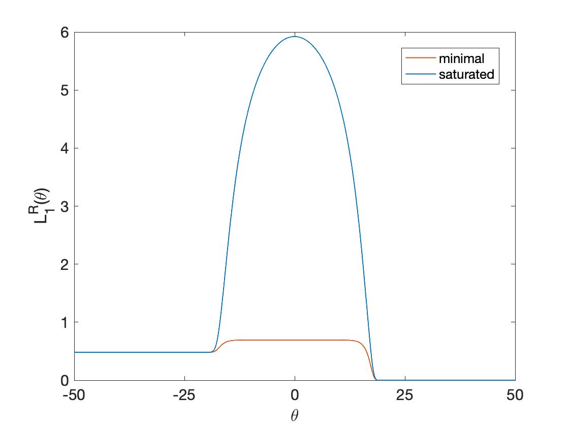
Figure 2: $L_{1}^{{\rm R}}(\theta)$ for minimal and saturated cases of ${\rm su(3)}$ at $\widehat{m}R=10^{-7}$.

The UV CFT’s in the two above cases, $[{\rm su(3)}]_{2}$ and ${\rm su(3)}_{2}$ both have a fractional supersymmetry with a conserved current of spin $8/5$ according to (106). In analogy with the ${\rm su(2)}$ Ising case, the massless particles which survive the flow can perhaps be interpreted as Goldstone particles for this broken fractional SUSY, however this suggestion clearly requires more investigation.

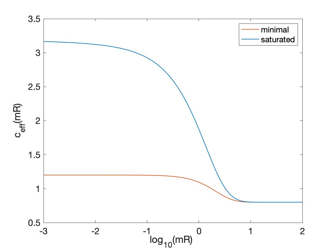
Figure 3: Minimal and saturated RG flows for ${\rm su(3)}$: $c(\widehat{m}R)$ vs $\log(\widehat{m}R)$ by solving TBA numerically. The IR central charge ($\widehat{m}R\to\infty$) is $c_{{\rm IR}}=4/5$. One clearly sees that both trajectories arrive to ${{\rm cft}_{{\rm IR}}}$ from the same direction, namely $T\overline{T}$.

Spanning the space of ${\widehat{K}}^{(0^{\prime})}$, i.e. $n_{1},n_{2}$, we find one additional exceptional case with $c_{{\rm UV}}=\tfrac{8}{5}$ where $(n_{1},n_{2})=(2,1)~{}{\rm or}~{}(1,2)$. One possible interpretation of this UV CFT is two copies of the IR minimal model each with $c_{{\rm IR}}=\tfrac{4}{5}$, however we cannot conclusively make this identification from the value of $c_{{\rm UV}}$ alone. These three UV completions, which we believe to be complete, are summarized in Table I.

$(n_{1},n_{2})$	$\widehat{x}_{1}=\widehat{x}_{2}$	$c_{{\rm UV}}$	${{\rm cft}_{{\rm UV}}}$
$(0,0)$	$\tfrac{\sqrt{5}+1}{2}$	$c_{{\rm UV}}=c_{{\rm IR}}=\tfrac{4}{5}$	${{\rm cft}_{{\rm UV}}}={{\rm cft}_{{\rm IR}}}=[{\rm su(3)}]_{1}$
$(1,1)$	$1$	$\tfrac{6}{5}$	${\rm Pf}_{2}$   “goldstino”   (minimal=diagonal)
$(2,1),(1,2)$	$\tfrac{\sqrt{5}-1}{2}$	$\tfrac{8}{5}$	$[{\rm su(3)}]_{1}\otimes[{\rm su(3)}]_{1}$ ?
$(2,2)$	$0$	$\tfrac{16}{5}$	${\rm su(3)}_{2}$   $({\rm saturated}$)

Table 1: su(3) results

VI.2 ${\rm su(4)}$ with $c_{{\rm IR}}=1$

In this case the $K$ matrices (65) are

$$K=-\tfrac{1}{2}\left(\begin{matrix}1&2&1\\ 2&2&2\\ 1&2&1\\ \end{matrix}\right),~{}~{}~{}~{}~{}{\widehat{K}}^{(0)}=\tfrac{1}{2}\left(\begin{matrix}3&2&1\\ 2&4&2\\ 1&2&3\\ \end{matrix}\right).$$ (93)

It turns out to be useful to introduce an $H$ matrix, as described in Section IVB, to simplify the form of ${\widehat{K}}^{(0)}$:

$$H=\tfrac{1}{2}\left(\begin{matrix}-1&0&1\\ 0&0&0\\ 1&0&-1\\ \end{matrix}\right),$$ (94)

which leads to

$${\widehat{K}}^{(0^{\prime})}={\widehat{K}}^{(0)}+H=\left(\begin{matrix}1&1&1\\ 1&2&1\\ 1&1&1\\ \end{matrix}\right).$$ (95)

Based on the above ${\widehat{K}}^{(0^{\prime})}$, we perform a complete classification based on the following space of ${\widehat{K}}$:

$${\widehat{K}}=\tfrac{1}{2}\left(\begin{matrix}n_{1}&n_{3}&n_{3}\\ n_{3}&n_{2}&n_{3}\\ n_{3}&n_{3}&n_{1}\\ \end{matrix}\right).$$ (96)

Spanning the space of $(n_{1},n_{2},n_{3})$ we find $11$ rational UV completions, which are summarized in Table II. The values $\widehat{x}_{1}=0.8019$ and $\widehat{x}_{1}=1.2469$ are solutions to the cubic equations

$$x^{3}-2x^{2}-x+1=0,~{}~{}~{}~{}x^{3}+x^{2}-2x-1=0$$ (97)

respectively.

Let us make some remarks on the results in Table II. For the generic cases, “minimal, diagonal, saturated” we can identify the ${{\rm cft}_{{\rm UV}}}$ based on arguments in Section IV. For the minimal case we know that $\Gamma_{\rm UV}=6/7$ (see Appendix). Since ${\rm Pf}_{2}={\rm su(4)}_{2}/{\rm su(4)}_{1}$, it is natural to expect that some of the additional cases with $c_{{\rm UV}}$ equal to integer multiples of $1/5$ are related to ${\rm su(3)}$ subgroups of ${\rm su(4)}$, such as ${\rm su(4)}_{2}/{\rm su(3)}_{1}$. We have tentatively indicated such identifications in the Table. However not all exceptional solutions can be explained this way, in particular $c_{{\rm UV}}=\tfrac{9}{7},\tfrac{13}{7}$, and other solutions which are multiples of $\tfrac{1}{5}$. Complete identification of the field content of UV theories in addition to their central charge $c_{{\rm UV}}$ is beyond the scope of this paper.

$(n_{1},n_{2},n_{3})$	$(\widehat{x}_{1}=\widehat{x}_{3},~{}\widehat{x}_{2})$	$c_{{\rm UV}}$	${{\rm cft}_{{\rm UV}}}$
$(0,0,0)$	$(2,3)$	$c_{{\rm UV}}=c_{{\rm IR}}=1$	${{\rm cft}_{{\rm UV}}}={{\rm cft}_{{\rm IR}}}=[{\rm su(4)}]_{1}$
$(2,0,0)$	$(1.2469,4.0489)$	$\tfrac{9}{7}$	?
$(2,4,0)$	$(\tfrac{\sqrt{5}+1}{2},\tfrac{\sqrt{5}+1}{2})$	$\tfrac{7}{5}$	?
$(0,2,1)$	$"$	$"$
$(1,2,1)$	$(1.2469,1.8019)$	$\tfrac{11}{7}$	$[{\rm su(4)}]_{2}$  ( minimal)
$(0,0,2)$	$(1,\tfrac{\sqrt{5}+1}{2})$	$\tfrac{9}{5}$	${\rm su(4)}_{2}/{\rm su(3)}_{1}$  ?
$(1,4,1)$	$(\tfrac{\sqrt{5}+1}{2},\tfrac{\sqrt{5}-1}{2})$	$"$
$(2,2,1)$	$(0.8019,2.2469)$	$\tfrac{13}{7}$	?
$(0,2,2)$	$(1,1)$	$2$	${\rm Pf}_{2}$   (diagonal )
$(2,4,1)$	$~{}"$	$"$
$(1,0,2)$	$(\tfrac{\sqrt{5}-1}{2},\tfrac{\sqrt{5}+1}{2})$	$\tfrac{11}{5}$	?
$(0,3,2)$	$(1,\tfrac{\sqrt{5}-1}{2})$	$"$
$(1,2,2)$	$(\tfrac{\sqrt{5}-1}{2},1)$	$\tfrac{12}{5}$	?
$(1,3,2)$	$(\tfrac{\sqrt{5}-1}{2},\tfrac{\sqrt{5}-1}{2})$	$\tfrac{13}{5}$	?
$(2,2,2)$	$(0,1)$	$4$	${\rm su(4)}_{2}/{\rm su(2)}_{1}={\rm su(4)}_{2}/u(1)$ ?
$(2,4,2)$	$(0,0)$	$5$	${\rm su(4)}_{2}$  (saturated )

Table 2: su(4) results

VI.3 Remarks on general su(n+1)

The coset $[{\rm su}(n+1)]_{1}$ deformed by the relevant field $\Phi_{{\rm rel}}^{(0)}$ in Section II, i.e. the field $\Phi^{(0)}_{{\rm rel};k=1}$ in (102), has $n$ particles with well-known masses and S-matrices. The complete S-matrices can be easily written down BCDS . From these, one can find the matrix $K$, which should be $K=-\mathcal{I}/(2-\mathcal{I})$ as above.

We have found that the $\widehat{K}$ which generates the RG flow from the IR CFT $[{\rm su}(n+1)]_{1}$ to the UV CFT $[{\rm su}(n+1)]_{2}$, i.e. the minimal case, is given by the following $n\times n$ matrix

$$\widehat{K}=\tfrac{1}{2}\left(\setcounter{MaxMatrixCols}{11}\begin{smallmatrix}1&1&1&1&1&\cdots&1&1&1&1&1\\ 1&2&2&2&2&\cdots&2&2&2&2&1\\ 1&2&3&3&3&\cdots&3&3&3&2&1\\ 1&2&3&4&4&\cdots&4&4&3&2&1\\ 1&2&3&4&5&\cdots&5&4&3&2&1\\ \vdots&\vdots&\vdots&\vdots&\vdots&\cdots&\vdots&\vdots&\vdots&\vdots&\vdots\\ 1&2&3&4&5&\cdots&5&4&3&2&1\\ 1&2&3&4&4&\cdots&4&4&3&2&1\\ 1&2&3&3&3&\cdots&3&3&3&2&1\\ 1&2&2&2&2&\cdots&2&2&2&2&1\\ 1&1&1&1&1&\cdots&1&1&1&1&1\end{smallmatrix}\right).$$ (98)

The above ${\widehat{K}}$ only describes the generic minimal flow. Based on the ${\rm su(3)},{\rm su(4)}$ cases above, we expect many more solutions with UV completions that are beyond the scope of this paper to attempt to classify.

VII Conclusions

We have shown how UV singularities in CFTs perturbed by the leading irrelevant operator $[T\overline{T}]_{1}=T\overline{T}/\pi^{2}$ can be resolved by including an infinite number of additional higher dimensional irrelevant operators $[T\overline{T}]_{s>1}$ with tuned couplings $\alpha_{s}$. By requiring integrability, we have argued that the classification of the possible UV completions is a well-defined problem, and we worked out many cases with diagonal S-matrices. We found many UV completions that were previously unknown, indicating that our proposed classification problem is feasible and constructive.

The UV completed theories are in principle completely defined by the S-matrices we propose. Our main tool is the TBA which can readily identify the central charge $c_{{\rm UV}}$ from the plateaux equations, as well as the conformal dimension of the relevant operator perturbation in the UV by carrying out a more detailed analysis of the TBA in the UV region which we will not perform in this article. This information will be essential to figure out an independent quantum field theory description of the UV field content and its field-theoretic relevant perturbations that lead to the RG flows to the IR that are implicit in the TBAs we propose. Thus the bottom up approach from a known IR CFT to a new UV CFT do not as yet completely determine the field content of the UV QFT, except in some cases, hence some of the “?” in Tables I and II. This is perhaps the main open question raised by this work. In fact one should entertain the possibility that the ${{\rm cft}_{{\rm UV}}}$ that we could not as yet completely identify may perhaps need to be eliminated by additional restrictions not considered here.

This work raises several other questions which could lead to interesting developments:

$\bullet$    We have clearly stated the restrictions we have imposed on our proposed classification problem that lead for instance to Tables I and II. Can these restrictions be relaxed or strengthened, which could lead to additional or less possible UV completions?

$\bullet$    Are there additional cases based on the $E_{8}$ magnetic spectrum of the Ising model which are beyond the 3 cases we have found, and can they be completely classified?

$\bullet$    Although the general ideas presented here extend to non-diagonal theories, it would be interesting to work out some examples in detail.

$\bullet$    How important is the role of symmetry? For some completions of the Ising model, the massless degrees of freedom, a Majorana fermion, were understood as Goldstone particles for broken supersymmetry. For some other cases we suggested that a broken fractional supersymmetry is playing a role. Can a generalized Goldstone theorem be developed? The fact that the maximal $c_{{\rm UV}}$ corresponds to the $G_{2}$ WZW model suggests that this may be possible.

$\bullet$    Are there interesting physical applications involving the Ising model in a vanishingly small magnetic field with non-zero $T\overline{T}$ perturbations? If so, then results from Section VB may be useful.

VIII Acknowledgements

We would like to thank the organizers and participants of the workshop APCTP focus program “Exact results on irrelevant deformations of QFTs” in October 2021 which led to this collaboration. AL benefitted from discussions with Denis Bernard and Giuseppe Mussardo. This work is supported in part by NRF grant (NRF- 2016R1D1A1B02007258) (CA).

Appendix A Current algebra CFTs and their cosets

Let $G$ denote a simply laced Lie group (ADE-type). The data we will need are the dimension of $G$, its rank, and its dual coxeter number $h^{*}$. They are related by ${\rm dim}\,G=(h^{*}+1)\,{\rm rank}\,G$. Let $G_{k}$ denote the WZW conformal field theory based on $G$ at level $k$, where $k$ is a positive integer KniZam ; GepWit . It has central charge

$$c(k)=\dfrac{k\,{\rm dim}G}{k+h^{*}}.$$ (99)

Then consider the GKO coset GKO

$$[G]_{k}=\dfrac{G_{k}\otimes G_{1}}{G_{k+1}},$$ (100)

with central charge $c([G]_{k})=c(k)+c(1)-c(k+1)$. For this series of cosets, the following models are integrable ABL :

$${\cal S}_{\lambda}={\cal S}_{[G]_{k}}+\lambda\int d^{2}x\,\Phi^{(0)}_{{\rm rel};k}$$ (101)

where $\Phi^{(0)}_{{\rm rel};k}$ is the coset field:

$$\Phi^{(0)}_{{\rm rel};k}=\left[\dfrac{(k;\circ)\otimes(1;\circ)}{(k+1;{\rm Adj})}\right]\,.$$ (102)

Above, $\circ$ and ${\rm Adj}$ denote the scalar and adjoint highest weight representations for the $G_{k}$ current algebra respectively. This relevant perturbation has dimension:

$${\rm dim}\left(\Phi^{(0)}_{{\rm rel};k}\right)=\dfrac{2(k+1)}{k+1+h^{*}}.$$ (103)

There is at least one UV completion we can anticipate based on conjectured massless flows in coset theories. For negative sign of $\lambda$, the spectrum is massive, and the S-matrices can be obtained from an RSOS restriction of the $G$ affine Toda theory ABL . For positive $\lambda$, the model is conjectured to be a massless flow from $[G]_{k}$ to $[G]_{k-1}$. The flow arrives to the $k-1$ theory via the irrelevant operator

$$\Phi^{(0)}_{{\rm irrel};k-1}=\left[\dfrac{(k-1;{\rm Adj})\otimes(1;\circ)}{(k;\circ)}\right]$$ (104)

of dimension $2(1+h^{*}/(k-1+h^{*}))$. Now, it is important to note that for $k=2$, the operator $(1;{\rm Adj})$ does not exist, thus for this massless flow the $[G]_{2}$ theory should arrive to the $[G]_{1}$ coset CFT via the $[T\overline{T}]_{s}$ operators. Thus in the UV the theory is described by

$${\cal S}_{\rm UV}={\cal S}_{[G]_{2}}+\lambda\int d^{2}x\,\Phi^{(0)}_{{\rm rel};2}$$ (105)

Based on these ingredients, in this paper we consider the model defined by (17), where ${{\rm cft}_{{\rm IR}}}=[G]_{1}$. One choice of $\alpha_{s}$ gives a UV completion which behaves as (105) in the UV, which we refer to as the minimal case. For this level $k=2$, $\Gamma_{\rm UV}={\rm dim}(\Phi^{(0)}_{{\rm rel};2})=6/(3+h^{*})$, and we indicate this in the body of the paper. Although this coset flow has been proposed already, the exact S-matrices and TBA have not previously been worked out at the level of detail presented in this paper.

We also wish to point out that the L,R chiral components of the primary field $\Phi^{(0)}_{{\rm irrel};k=2}$ are non-local conserved currents $J_{\rm fsusy}$ for a fractional supersymmetry with dimension (and spin)

$$\Delta\left(J_{\rm fsusy}\right)=1+\dfrac{h^{*}}{2+h^{*}}.$$ (106)

This symmetry also exists in the complete series of cosets $G_{\ell}\otimes G_{2}/G_{\ell+2}$ for all $\ell$, including the WZW model $G_{2}$ which arises in the $\ell\to\infty$ limit. For $G={\rm su(2)}$, where $h^{*}=2$, this spin $3/2$ current generates an ${\cal N}=1$ supersymmetry.

In sorting out the $UV$ CFT’s it is useful to introduce a free field content for the current algebra $G_{k}$. The cosets can then be described by the introduction of background charges for the bosons. One needs ${\rm rank}\,G$ bosons and some additional non-abelian parafermions based on $G_{k}$:

$${\rm Pf}_{k}=G_{k}/u(1)^{{\rm rank}G},~{}~{}~{}~{}~{}~{}~{}c({\rm Pf}_{k})={\rm rank}G\,\left(\dfrac{h^{*}(k-1)}{k+h^{*}}\right).$$ (107)

Throughout this paper we do not display the $G$ dependence of ${\rm Pf}_{2}$ since this evident from the context.

It is interesting to note that comparing central charges, one can potentially make the identification

$${\rm Pf}_{2}=G_{2}/G_{1},~{}~{}~{}c=\dfrac{h^{*}{\rm rank}\,G}{2+h^{*}}.$$ (108)

We have not studied whether the above is an exact equivalence, nevertheless we will use this insight for the ${\rm su(4)}$ cases above with $G_{2}/H_{1}$, where $H$ is a subgroup of $G$, to tentatively propose the identification of some UV completions. For the $[T\overline{T}]_{s}$ deformations we are here mainly concerned with the ${\rm Pf}_{k=2}$ case. Note that for $G={\rm su(2)}$ at level $k=2$, the ${\rm Pf}_{2}$ parafermion is just a Majorana fermion with $c=\tfrac{1}{2}$.

References

- (1) S. Weinberg, Critical Phenomena for Field Theorists, In Zichichi, Antonino (ed.). Understanding the Fundamental Constituents of Matter. The Subnuclear Series. 14. pp. 1-52, 1978; Phys. Rev. D81 (2010) 083535.
- (2) A. B. Zamolodchikov, Irreversibility of the flux of the renormalization group in a 2D field theory, Pis’ma Eksp. Teor. Fiz. 43 (1986) 565.
- (3) C. Vafa, The string landscape and the swampland, arXiv:hep-th/0509212.
- (4) F. A. Smirnov and A. B. Zamolodchikov, On the space of integrable quantum field theories, Nucl. Phys. B915 (2017) 363, arXiv:1608.05499.
- (5) A Cavaglià, S Negro, I.M. Szecsenyi, R Tateo, -deformed 2D quantum field theories, JHEP 10 (2016) 112, arXiv:1608.05534 [hep-th].
- (6) A. B. Zamolodchikov, Expectation value of composite field T anti-T in two-dimensional quantum field theory, hep-th/0401146.
- (7) S. Dubovsky, V. Gorbenko, and M. Mirbabayi, Asymptotic fragility, near AdS2 holography and , JHEP 09 (2017) 136, arXiv:1706.06604 [hep-th].
- (8) S. Dubovsky, V. Gorbenko, and G. Hernandez-Chifflet, partition function from topological gravity, JHEP 09 (2018) 158, arXiv:1805.07386 [hep-th].
- (9) L. McGough, M. Mezei, H. Verlinde, Moving the CFT into the bulk with , JHEP 10 (2018) 1, arXiv:1611.03470 [hep-th].
- (10) J. Cardy, The deformation of quantum field theory as random geometry, JHEP 10 (2018) 186, arXiv:1801.06895 [hep-th].
- (11) R. Conti, L. Iannella, S. Negro, and R. Tateo, Generalized Born-Infeld models, Lax operators and the perturbation, JHEP 11 (2018) 007, arXiv:1806.11515 [hep-th].
- (12) R. Conti, S. Negro, and R. Tateo, The perturbation and its geometric interpretation, JHEP 02 (2019) 085, arXiv:1809.09593 [hep-th].
- (13) A. B. Zamolodchikov, Integrable Field Theory from Conformal Field Theory, Adv. Stud. in Pure Math. 19 (1989) 641.
- (14) G. Mussardo, Statistical Field Theory. An Introduction to Exactly Solved Models in Statistical Physics, Oxford University Press, 2010.
- (15) Al. B. Zamolodchikov, From tricritical Ising to critical Ising by thermodynamic Bethe ansatz, Nucl. Phys. B358 (1991) 524.
- (16) A. B. Zamolodchikov and Al. B. Zamolodchikov, Massless factorized scattering and sigma models with topological terms, Nucl. Phys. B379 (1992) 602.
- (17) A. LeClair, deformation of the Ising model and its ultraviolet completion, J. Stat. Mech. (2021) 113104, arXiv:2107.02230 [hep-th].
- (18) C. Ahn, C. Kim, C. Rim, and Al. B. Zamolodchikov, RG flows from super-Liouville theory to critical Ising model, Phys. Lett. B541 (2002) 194, arXiv:hep-th/020621 .
- (19) L. Castillejo, R.H. Dalitz and F.J. Dyson, Phys. Rev. 101 (1956) 453.
- (20) A. LeClair, Thermodynamics of perturbations of some single particle theories, J. Phys. A: Math. Theor. 55 185401, arXiv:2105.08184 [hep-th].
- (21) G. Hernández-Chifflet, S. Negro, and A. Sfondrini, Flow Equations for Generalized Deformations, Phys. Rev. Lett. 124 (2020) 200601, arXiv:1911.12233 [hep-th].
- (22) B. Doyon, J. Durnin, and T. Yoshimura, The Space of Integrable Systems from Generalised -Deformations, arXiv:2105.03326 [hep-th].
- (23) G. Camilo, T. Fleury, M. Lencsés, S. Negro, and A. Zamolodchikov, On factorizable S-matrices, generalized TTbar, and the Hagedorn transition, JHEP 10 (2021) 062, arXiv:2106.11999 [hep-th].
- (24) L. Córdova, S. Negro, and F. Schaposnik Massolo, Thermodynamic Bethe Ansatz past turning points: the (elliptic) sinh-Gordon model, JHEP 01 (2022) 035, arXiv:2110.14666 [hep-th].
- (25) Al. B. Zamolodchikov, Thermodynamic Bethe Ansatz in relativistic models: scaling 3-state Potts and Lee-Yang models, Nucl. Phys. B342 (1990) 695.
- (26) T. Klassen and E. Melzer, The thermodynamics of purely elastic scattering theories and conformal perturbation theory, Nucl. Phys. B350 (1991) 635.
- (27) A. B. Zamolodchikov, Nucl. Phys. B358 (1991) 524.
- (28) F. Ravanini, Theormodynamic Bethe Ansatz for coset models perturbed by their operator, Phys. Lett. B282 (1992) 73, arXiv:hep-th/9202020.
- (29) C. Ahn, D. Bernard and A. LeClair, Fractional supersymmetry in perturbed coset CFTs and integrable soliton theory, Nucl. Phys. B346 (1990) 409.
- (30) H. W. Braden, E. Corrigan, P. E. Dorey, and R. Sasaki, Affine Toda field theory and exact S-matrices, Nucl. Phys. B338 (1990) 689.
- (31) Al. B. Zamolodchikov, On the thermodynamic Bethe ansatz equations for reflectionless ADE scattering theories, Phys. Lett. B253 (1991) 391.
- (32) V. G. Knizhnik and A. B. Zamolodchikov, Current algebras and Wess-Zumino model in two dimensions, Nucl. Phys. B247 (1984) 83.
- (33) D. Gepner and E. Witten, String theory on group manifolds, Nucl. Phys. B278 (1986) 493.
- (34) P. Goddard, A. Kent, and D. Olive, Virasoro algebras and coset space models, Phys. Lett. B152 (1985) 88.