Casimir effect between spherical objects: proximity-force approximation and beyond using plane waves

Abstract

For the Casimir interaction between two nearby objects, the plane-wave basis proves convenient for numerical calculations as well as for analytical considerations leading to an optical interpretation of the relevant scattering processes of electromagnetic waves. We review work on the proximity-force approximation and corrections to it within the plane-wave basis for systems involving spherical objects. Previous work is extended by allowing for polarization mixing during the reflection at a sphere. In particular, explicit results are presented for perfect electromagnetic conductors. Furthermore, for perfect electric conductors at zero temperature, it is demonstrated that beyond the leading-order correction to the proximity-force approximation, terms of half-integer order in the distance between the sphere surfaces appear.

I Introduction

Even though Casimir’s original calculation of the force between two objects due to the electromagnetic vacuum considered two parallel plates Casimir (1948), most experiments involve a sphere or a spherical lens, often placed close to a plate (see, e.g., Refs. Klimchitskaya and Mostepanenko, 2006; Klimchitskaya et al., 2009; Decca et al., 2011; Lamoreaux, 2011; Klimchitskaya and Mostepanenko, 2020; Mostepanenko and Klimchitskaya, 2020; Gong et al., 2021 for reviews). The advantage of the sphere is that no special care needs to be taken to avoid misalignment. Recently, experiments involving two spheres have been carried out as well Ether jr. et al. (2015); Garrett et al. (2018); Pires et al. (2021). However, the strength of the Casimir force is limited by the sphere radius. For most practical purposes, the sphere radius therefore is chosen to be very large compared to the distance to the other object. For the majority of experiments, the aspect ratio between sphere radius and surface-to-surface distance lies between 100 and 5000 Hartmann et al. (2018). A notable exception is an experiment involving two spheres with an aspect ratio smaller than 10 where optical tweezers are used in order to measure a rather weak Casimir force Ether jr. et al. (2015); Pires et al. (2021).

For large aspect ratios, the force between the two involved objects can be obtained to a very good approximation by dividing the opposing surfaces into parallel surface elements and summing up the free energy for the respective distances. This approximation was first introduced by Derjaguin Derjaguin (1934) and the term proximity force was coined by Błocki et al. Błocki et al. (1977) leading to the often used term proximity-force approximation (PFA). While the results of PFA are in many cases sufficient to analyze experimental data, the increasing experimental precision Krause et al. (2007); Liu et al. (2019a, b) and the Drude-plasma controversy Decca et al. (2007); Mostepanenko (2021) motivate to go beyond PFA. In special cases, it is possible to obtain analytical expressions for the leading order corrections to PFA, for instance by developing a derivative expansion of the interaction energy Fosco et al. (2011, 2014). However, in general one needs to resort to numerical techniques, particularly when dealing with moderate values for the aspect ratio or when a higher precision is required.

There exist a number of numerical approaches to the Casimir effect, some of them capable to handle rather general geometries Oskooi et al. (2010); Reid and Johnson (2015) and others adapted to specific shapes of the involved objects.Hartmann and Ingold (2020) Here, we will concentrate on setups containing two spheres or a sphere and a plate. Using a spherical wave basis may appear as quite natural and recently it became indeed possible to push the limits of this method well into the experimentally relevant regime Hartmann et al. (2017, 2018). It should be kept in mind though that for a setup consisting of two spheres, two spherical wave bases are actually needed, each of them centered at one of the spheres. As a consequence, it is necessary to transform between these two bases. Bispherical coordinates might appear as an alternative and they have in fact been used to derive exact expressions for the Casimir force between two spheres of equal radii as well as between a plane and a sphere in the high-temperature limit Bimonte and Emig (2012).

More recently, it became clear that the use of a plane-wave basis can be advantageous Spreng et al. (2020); Nunes et al. (2021); Spreng (2021), in particular when the aspect ratio becomes large as is the case in most experiments. In view of the proximity-force approximation where a more general geometry is locally approximated by a plane-plane geometry, the advantages of the plane-wave basis are comprehensible. An analysis of experimental data by numerical techniques based on plane waves is presented in Ref. Bimonte et al., 2021. The plane-wave approach has also been employed to produce data for another article in this volume Schoger et al. .

The plane-wave basis is not only useful for numerical computations but also in analytical calculations. The proximity-force approximation for two spheres has been derived by means of the scattering approach to the Casimir effect Lambrecht et al. (2006); Emig et al. (2007); Ingold and Lambrecht (2015) as an asymptotic result using the plane-wave basis Spreng et al. (2018). Furthermore, extending this approach, corrections to PFA have been obtained Henning et al. (2019, 2021). In the high-temperature limit, using the plane-wave basis, an exact expression for the Casimir free energy between two spheres of arbitrary radii was found Schoger and Ingold (2021). Some of the results had been at least partially derived before by other means for the plane-sphere geometry at zero temperature Bordag and Nikolaev (2008); Emig (2008); Maia Neto et al. (2008); Teo et al. (2011); Bimonte et al. (2012); Teo (2013) and in the high-temperature limit Canaguier-Durand et al. (2012) as well as for the sphere-sphere geometry at zero temperature Teo (2012) and for high temperatures Bimonte and Emig (2012); Fosco et al. (2016). On the other hand, particularly for large aspect ratios, a calculation based on plane waves offers the opportunity for physical insights in terms of the concepts of geometrical optics and its semiclassical corrections.

In the following, we will discuss the Casimir interaction between spherical objects in vacuum including the sphere-plane geometry as a limiting case from the point of view of plane waves. While part of the paper will review previous work, we will also present some new results. In particular, we will derive the PFA expression in the plane-wave basis for polarization-mixing reflection at the spheres, thereby generalizing previous work. Furthermore, we will point out the appearance of so far unexpected corrections to the PFA result.

The paper is organized as follows. Section II introduces the scattering approach to the Casimir free energy within the plane-wave basis. The asymptotic expansion of the reflection coefficients for large radii is developed in Sec. III. In Sec. IV, the Casimir free energy is evaluated in the saddle-point approximation to obtain the PFA in the presence of polarization-mixing reflection. The leading-order correction to PFA is discussed in Sec. V, where explicit results are given for perfect electromagnetic conductors at zero temperature. Finally, Sec. VI explores the origin of the next-to-leading order correction to PFA. Concluding remarks are given in Sec. VII.

II Scattering approach in the plane-wave basis

II.1 General expression for the Casimir free energy

When an object is placed into electromagnetic vacuum thereby acting as a scatterer, it will give rise to a phase shift during the scattering process and, as a consequence, to a change in the vacuum energy. If instead of a single object two objects are considered, the Casimir energy is obtained by isolating the distance-dependent part of the vacuum energy. The object describing the relevant part of the scattering process in the latter case is the round-trip operator

$$\mathcal{M}=\mathcal{R}_{2}\mathcal{T}_{21}\mathcal{R}_{1}\mathcal{T}_{12}$$ (1)

containing reflections at the two objects described by the operators $\mathcal{R}_{1}$ and $\mathcal{R}_{2}$ and translations between the two objects in terms of the operators $\mathcal{T}_{21}$ and $\mathcal{T}_{12}$.

The Casimir energy then reads

$$E=\frac{\hbar}{2\pi}\int_{0}^{\infty}d\omega\text{Im}\log\det(1-\mathcal{M}(\omega))\,.$$ (2)

This expression is valid not only for the unitary case but also in the presence of dissipative channels Guérout et al. (2018). In order to avoid resonances on the real frequency axis, it is convenient to perform a Wick transformation and to express the Casimir energy in terms of imaginary frequencies $\xi=-i\omega$. Then, (2) becomes

$$E=\frac{\hbar}{2\pi}\int_{0}^{\infty}d\xi\mathfrak{F}(\xi)$$ (3)

with

$$\mathfrak{F}(\xi)=\log\det\big{(}1-\mathcal{M}(\xi)\big{)}\,.$$ (4)

In the following, we will always make use of imaginary frequencies unless stated otherwise. At finite temperatures, thermal fluctuations of the electromagnetic field have to be accounted for as well. This can be done within the Matsubara formalism where the Casimir free energy at temperature $T$ is found as

$$\mathcal{F}=\frac{k_{\mathrm{B}}T}{2}\sum_{n=-\infty}^{\infty}\mathfrak{F}(|\xi_{n}|)$$ (5)

with the Matsubara frequencies $\xi_{n}=2\pi nk_{\mathrm{B}}T/\hbar$. Making use of the mathematical identity $\log\det(1-\mathcal{M})=\text{tr}\log(1-\mathcal{M})$ we can expand the logarithm and decompose the free energy into contributions of $r$ round-trips between the two scatterers as

$$\mathfrak{F}(\xi)=-\sum_{r=1}^{\infty}\frac{\text{tr}\mathcal{M}^{r}(\xi)}{r}\,.$$ (6)

The evaluation of the trace requires the choice of an appropriate basis. While spherical waves are practical for distances large compared to the diameter of the objects, plane waves turn out to be more suitable for short distances Spreng et al. (2018) and will be chosen in the following.

We characterize the plane waves in our basis by its wave vector and polarization. It is convenient to decompose the wave vector into its projection $\mathbf{k}$ onto the plane perpendicular to the axis connecting the two scattering objects. The wave vector component $\kappa$ along the axis is taken imaginary as we did with the frequency $\xi$ so that the dispersion relation becomes

$$\kappa=\left(\frac{\xi^{2}}{c^{2}}+k^{2}\right)^{1/2}$$ (7)

with the modulus $k$ of the transverse wave vector $\mathbf{k}$. Since $\kappa$ is positive, we denote the sense of propagation by a sign $\phi=\pm$.

The polarization $p$ of the plane wave is defined with respect to the Fresnel plane (F). As shown in Fig. 1, the Fresnel plane is spanned by the axis connecting the two scattering objects, i.e. the $z$-axis in the figure, and the incident real wave vector $\mathbf{K}_{\text{in}}$. We distinguish between transverse magnetic ($p=\mathrm{TM}$) and transverse electric ($p=\mathrm{TE}$) modes, where the electric field is parallel or perpendicular to the Fresnel plane, respectively.

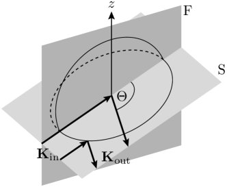
Figure 1: The Fresnel plane (F) is spanned by the $z$-axis and the incident wave vector $\mathbf{K}_{\text{in}}$ while the scattering plane (S) is spanned by the incident wave vector and the wave vector $\mathbf{K}_{\text{out}}$ of the reflected wave. The scattering angle is denoted by $\Theta$.

An incident plane wave of our basis is denoted in the angular spectral representation Nieto-Vesperinas (2006) as $|\mathbf{k},p,\phi\rangle$. Here, we omit the imaginary frequency $\xi$ which is conserved through the complete scattering process. As $\kappa$ is defined through the dispersion relation (7), we do not need to include it in our notation. The specification of the plane wave is completed by the polarization $p$ and the propagation direction indicated by the sign $\phi=\pm$.

We are now in a position to explicitly express the trace appearing in the round-trip expansion (6) of the free energy in terms of the plane-wave basis. The trace over the $r$-th power of the round-trip operator reads

$$\mathrm{tr}\mathcal{M}^{r} =\sum_{p_{1},\ldots,p_{2r}}\int\frac{\mathrm{d}\mathbf{k}_{1}\ldots\mathrm{d}\mathbf{k}_{2r}}{(2\pi)^{4r}}\prod_{j=1}^{r}\mathrm{e}^{-\kappa_{2j}\mathcal{L}}\mathrm{e}^{-\kappa_{2j-1}\mathcal{L}}$$ (8)

$$\quad\times\langle\mathbf{k}_{2j+1},p_{2j+1},-|\mathcal{R}_{2}|\mathbf{k}_{2j},p_{2j},+\rangle$$

$$\quad\times\langle\mathbf{k}_{2j},p_{2j},+|\mathcal{R}_{1}|\mathbf{k}_{2j-1},p_{2j-1},-\rangle\,,$$

where cyclic indices $2r+1\equiv 1$ were introduced to account for the trace. The product in (8) contains exponential factors arising from the translation operators $\mathcal{T}_{ij}$ in (1) which in the plane-wave basis are diagonal and describe the translation over the distance $\mathcal{L}$ between the two scattering objects. The reflection matrix elements will in general be nondiagonal and depend on the details of the objects scattering the electromagnetic waves. So far, expression (8) is general. In the next section, we specialize to spherical objects which will allow us to obtain explicit expressions for the reflection matrix elements.

II.2 Reflection matrix elements

The scattering of electromagnetic waves at a sphere can be solved analytically Mie (1908) and Mie scattering is discussed in various textbooks van de Hulst (1981); Bohren and Huffman (2004). We therefore concentrate in this section only on aspects relevant for our purposes.

In the spherical-wave basis characterized by the angular momentum eigenvalues $\ell$ and $m$ as well as the polarization $P=\text{E},\text{M}$, which can be electric or magnetic, respectively, the matrix elements of the reflection operator are given by

$$\langle\ell^{\prime},m^{\prime},P^{\prime},\mathrm{out}|\mathcal{R}|\ell,m,P,\mathrm{reg}\rangle=r_{\ell}^{P^{\prime}P}(i\tilde{\xi})\delta_{\ell,\ell^{\prime}}\delta_{m,m^{\prime}}$$ (9)

with the size parameter

$$\tilde{\xi}=\frac{\xi R}{c}\,.$$ (10)

Here, $R$ is the sphere radius and $c$ denotes the speed of light. We use ‘reg’ to refer to a spherical wave which is regular at the sphere center while ‘out’ refers to an outgoing spherical wave van de Hulst (1981).

Due to the spherical geometry, $\ell$ and $m$ are conserved during the scattering process. While mostly isotropic materials are discussed in the literature, where also the polarization is conserved, we will allow here for the more general case where the polarization may change as a result of the scattering at the sphere. Such a situation is encountered for spheres made of a bi-isotropic material characterized by the constitutive relations Sihvola and Lindell (1991)

$$\mathbf{D} =\varepsilon\mathbf{E}+\alpha\mathbf{H}$$ (11)

$$\mathbf{B} =\mu\mathbf{H}+\beta\mathbf{E}$$

relating the electric displacement $\mathbf{D}$ and the magnetic induction $\mathbf{B}$ to the electric field $\mathbf{E}$ and the magnetic field $\mathbf{H}$. Among the quantities characterizing the material, $\varepsilon$ and $\mu$ are assumed to be scalars while $\alpha$ and $\beta$ are pseudoscalars. An important class of materials described by such relations are chiral materials Condon (1937) where $\alpha=-\beta$. Taking the prefactors to infinity, perfect electromagnetic conductors (PEMC) Lindell and Sihvola (2005) interpolating between perfect electric conductors ($\varepsilon\to\infty$) and perfect magnetic conductors ($\mu\to\infty$) are also covered by (11), if one takes $\alpha=\beta$. PEMC have recently been discussed in the context of the Casimir effect Rode et al. (2018).

As already pointed out above, we want to make use of the plane-wave basis. The Mie scattering amplitudes $S_{p^{\prime}p}$ describe the scattering of a plane wave with polarization $p$ by the sphere into a plane wave with polarization $p^{\prime}$. The scattering geometry is defined by the in- and outgoing wave vectors spanning the scattering plane indicated by S in Fig. 1. It is also with respect to this plane that the polarization is defined. The two wave vectors define a scattering angle $\Theta$ also shown in Fig. 1. For the imaginary frequency $\xi$ and wave-vector component $\kappa$ introduced earlier, the scattering angle is determined through

$$\cos(\Theta)=-\frac{c^{2}}{\xi^{2}}(\mathbf{k}_{\text{out}}\cdot\mathbf{k}_{\text{in}}+\kappa_{\text{out}}\kappa_{\text{in}})\,.$$ (12)

Explicit expressions for the Mie scattering amplitudes have been derived in Ref. Bohren, 1974. With our notation for the reflection matrix elements (9), they are given by

$$S_{\mathrm{TE},\mathrm{TE}}(\Theta) =-\sum_{\ell=1}^{\infty}\frac{2\ell+1}{\ell(\ell+1)}(\tau_{\ell}r_{\ell}^{\mathrm{M}\mathrm{M}}+\pi_{\ell}r_{\ell}^{\mathrm{E}\mathrm{E}})$$ (13)

$$S_{\mathrm{TM},\mathrm{TM}}(\Theta) =-\sum_{\ell=1}^{\infty}\frac{2\ell+1}{\ell(\ell+1)}(\tau_{\ell}r_{\ell}^{\mathrm{E}\mathrm{E}}+\pi_{\ell}r_{\ell}^{\mathrm{M}\mathrm{M}})$$ (14)

$$S_{\mathrm{TM},\mathrm{TE}}(\Theta) =i\sum_{\ell=1}^{\infty}\frac{2\ell+1}{\ell(\ell+1)}(\tau_{\ell}r_{\ell}^{\mathrm{E}\mathrm{M}}+\pi_{\ell}r_{\ell}^{\mathrm{M}\mathrm{E}})$$ (15)

$$S_{\mathrm{TE},\mathrm{TM}}(\Theta) =-i\sum_{\ell=1}^{\infty}\frac{2\ell+1}{\ell(\ell+1)}(\tau_{\ell}r_{\ell}^{\mathrm{M}\mathrm{E}}+\pi_{\ell}r_{\ell}^{\mathrm{E}\mathrm{M}})\,.$$ (16)

While in the usual case of isotropic spheres only the first two scattering amplitudes are non-vanishing, we need to account for all four of them as we are dealing with bi-isotropic spheres. The scattering amplitudes not only depend on the reflection matrix elements (9) but also contain the scattering geometry through the angular functions Bohren and Huffman (2004)

$$\pi_{\ell} =\frac{P_{\ell}^{1}\big{(}\cos(\Theta)\big{)}}{\sin(\Theta)}$$ (17)

$$\tau_{\ell} =\frac{dP_{\ell}^{1}\big{(}\cos(\Theta)\big{)}}{d\Theta}\,,$$ (18)

where $P_{\ell}^{1}$ are associated Legendre polynomials DLMF .

So far, the scattering plane has been used in the calculations. However, for our purposes in a two-sphere setup, the Fresnel plane is more convenient. In a last step, we thus have to transform the results from the scattering plane to the Fresnel plane indicated as S and F, respectively, in Fig. 1. The matrix elements needed for this basis change can be found in Refs. Mishchenko, 2000 and Messina et al., 2015. Finally, one arrives at the reflection matrix element in the plane-wave basis

$$\langle\mathbf{k}_{j},p_{j}|\mathcal{R}|\mathbf{k}_{i},p_{i}\rangle =\frac{2\pi c}{\xi\kappa_{j}}\big{[}AS_{p_{j}p_{i}}+(-1)^{p_{j}+p_{i}}BS_{\bar{p}_{j}\bar{p}_{i}}$$ (19)

$$\quad-(-1)^{p_{j}}CS_{\bar{p}_{j}p_{i}}+(-1)^{p_{i}}DS_{p_{j}\bar{p}_{i}}\big{]}\,,$$

where the polarization of the in- and outgoing plane waves is defined with respect to the Fresnel plane and the transverse wave vector is taken with respect to the axis connecting the two spheres. In the exponents, $p$ takes the values $1$ and $2$ for polarizations TE and TM, respectively, and the bar over a polarization refers to the other polarization, i.e. $\bar{p}=\mathrm{TM}$ if $p=\mathrm{TE}$ and vice versa. The coefficients $A,B,C,$ and $D$ are functions of the three-dimensional wave vectors, e.g. $A=A(\mathbf{K}_{j},\mathbf{K}_{i})$. Since we will not need the complete expression of these coefficients in the following, we refer the reader interested in more details to Ref. Spreng et al., 2018 and in particular to appendix A of that paper for explicit expressions for the coefficients $A,B,C,$ and $D$.

III Scattering at large spheres

The proximity-force approximation can be obtained as leading-order term in an asymptotic expansion for large sphere radii $R_{1}$ and $R_{2}$ and corrections are given by higher-order terms. An important ingredient are the reflection matrix elements for a sphere which we will expand in this section for large radii $R$. For real frequencies, the leading-order term of the reflection matrix elements corresponds to the geometrical optics limit which was extensively discussed e.g. in Refs. Nussenzveig, 1969; van de Hulst, 1981; Nussenzveig, 1992; Grandy Jr, 2000. In order to evaluate corrections to the proximity-force approximation, we will also need to consider at least the leading correction to the reflection matrix elements which gives rise to diffractive corrections. As a consequence, while the PFA result can be obtained within geometrical optics, corrections to PFA will contain contributions from geometrical optics as well as from diffraction.

When expanding the reflection matrix elements, we will need to assume that the radius $R$ is large compared to other length scales of the problem, which in our case is the wave number $\xi/c$. While for non-zero values of $\xi$ it is sufficient to take the limit of a large size parameter (10), we have to consider the case $\xi=0$ separately.

III.1 Reflection coefficients for finite frequencies

In the expansion of the scattering amplitudes (13)–(16) appearing in (19) for large sphere radius, the localization principle van de Hulst (1981) plays an important role. According to this principle, the scattering of a ray with an impact parameter $b$ is dominated by angular momenta of the order of $\xi b/c$. Applying Debye’s expansion DLMF to the reflection coefficients $r_{\ell}^{P^{\prime}P}$ defined through (9), the asymptotic expansion in the multipole basis is already completed. The resulting expressions for the Mie coefficients in the isotropic case have been used e.g. in Ref. Teo, 2013 to obtain the leading correction to the proximity-force approximation in the plane-sphere geometry.

Within the plane-wave basis, we need to go one step further and evaluate the sum over the angular momenta in (13)–(16). Since the procedure for real frequencies is well known from textbooks and can be carried over to imaginary frequencies without any difficulties, we will restrict ourselves to outlining the main ideas. In view of the localization principle, we need to account for angular momenta $\lambda=\ell+1/2\lesssim\tilde{\xi}$. Since the size parameter $\tilde{\xi}$ defined in (10) for a fixed frequency $\xi$ becomes large for large radius $R$, we can approximate the sums in (13)–(16) by integrals over $\lambda$. In addition, an asymptotic expansion of the angular functions (17) and (18) for large orders $\ell$ is used. Then, the dominant contribution to the integral can be obtained by means of the saddle-point approximation with the saddle point given by

$$\lambda_{\text{sp}}=i\tilde{\xi}\cos\left(\frac{\Theta}{2}\right)\,.$$ (20)

For real frequencies, the saddle point corresponds to a ray hitting the sphere with an impact parameter $b=\lambda_{\text{sp}}c/i\xi=R\cos(\Theta/2)$ as depicted in Fig. 2, where $\Theta$ is the scattering angle.

Figure 2: Scattering geometry at a sphere of radius $R$ for a scattering angle $\Theta$ (cf. Fig. 1). The corresponding impact parameter $b$ in ray optics is given by $R\cos(\Theta/2)$.

After proceeding as for real frequencies Grandy Jr (2000), one finds for the scattering amplitudes for imaginary frequencies

$$S_{p^{\prime}p}(\Theta)=\frac{\tilde{\xi}}{2}e^{2\tilde{\xi}\sin(\Theta/2)}\tilde{r}_{p^{\prime}p}(\Theta)$$ (21)

with

$$\tilde{r}_{p^{\prime}p}(\Theta)=r_{p^{\prime}p}\left(\frac{\pi-\Theta}{2}\right)\left[1+\frac{s_{p^{\prime}p}}{\tilde{\xi}}+\mathcal{O}\left(\tilde{\xi}^{-2}\right)\right]\,.$$ (22)

The exponential term in (21) accounts for the difference in path lengths between a ray reflected at the sphere surface and a ray going to the sphere origin and being deflected there by the scattering angle $\Theta$ as depicted in Fig. 2. The latter ray is relevant for us because the origin of the sphere was chosen as origin of the reference frame for the plane-wave basis.

In (22), $r_{p^{\prime}p}$ are the reflection coefficients at a plane evaluated at an angle of incidence $(\pi-\Theta)/2$ corresponding to a scattering angle $\Theta$ as can be seen from Fig. 2. The leading-order term for large radii then does not depend on the curvature of the sphere. In the absence of polarization mixing, the reflection coefficients correspond to the well-known Fresnel reflection coefficients Bohren and Huffman (2004). For bi-isotropic materials, the reflection coefficients can be found in Ref. Lindell et al., 1994. The leading corrections are given by $s_{p^{\prime}p}$ and explicit expression have been determined in Refs. Grandy Jr, 2000 and Khare, 1975 for isotropic materials. However, the expressions given in the two references do not agree and are also inconsistent with numerical results. Therefore, for reference, we give the explicit expressions derived in Ref. Spreng, 2021 which were checked against the numerical results. Introducing the abbreviations $s\equiv\sin(\Theta/2)$ and $c\equiv\cos(\Theta/2)$, the corrections for a dielectric nonmagnetic material with index of refraction $n=\epsilon^{1/2}$ read

$$s_{\mathrm{TE},\mathrm{TE}} =\frac{1-2s^{2}}{2s^{3}}+\frac{1}{s}\frac{1}{c^{2}+s(n^{2}-c^{2})^{1/2}}$$ (23)

$$\quad-\frac{2n^{2}-c^{2}}{2(n^{2}-c^{2})^{3/2}}$$

$$s_{\mathrm{TM},\mathrm{TM}} =-\frac{1}{2s^{3}}+\frac{1}{s}\frac{1}{c^{2}-s(n^{2}-c^{2})^{1/2}}$$ (24)

$$\quad-\frac{c^{2}}{s^{3}}\frac{2n^{4}s^{2}-n^{2}c^{2}(1+s^{2}-s^{4})+c^{6}}{(n^{2}-c^{2})(n^{2}s^{2}-c^{2})^{2}}$$

$$\quad+\frac{n^{2}}{2(n^{2}-c^{2})^{3/2}}\frac{2n^{4}-n^{2}c^{2}(1+c^{2})-c^{4}}{(n^{2}s^{2}-c^{2})^{2}}\,.$$

For perfect reflectors, which we will always assume to be made of a perfectly electric conductor, $n\to\infty$ and all terms except for the first one in each case vanish and the results agree with Refs. Grandy Jr, 2000 and Khare, 1975 in that limit.

As a definite example where polarization mixing occurs during a reflection, we consider a sphere made of a perfect electromagnetic conductor (PEMC) Ruppin (2006), a model introduced above. PEMC are characterized by an angle $\theta$ (not to be confused with the scattering angle $\Theta$) which describes the transition from a perfect electric conductor with $\theta=0$ to a perfect magnetic conductor with $\theta=\pi/2$. The reflection coefficients including the first correction in $1/\tilde{\xi}$ are given by

$$\tilde{r}_{\mathrm{TE},\mathrm{TE}} =-\cos(2\theta)$$ (25)

$$\quad-\frac{1}{\tilde{\xi}}\left(\frac{1-2s^{2}}{2s^{3}}\cos(2\theta)+\frac{c^{2}}{s^{3}}\sin^{2}(\theta)\right)+O(\tilde{\xi}^{-2})$$

$$\tilde{r}_{\mathrm{TM},\mathrm{TM}} =\cos(2\theta)$$ (26)

$$\quad+\frac{1}{\tilde{\xi}}\left(\frac{1-2s^{2}}{2s^{3}}\cos(2\theta)-\frac{c^{2}}{s^{3}}\cos^{2}(\theta)\right)+O(\tilde{\xi}^{-2})$$

$$\tilde{r}_{\mathrm{TE},\mathrm{TM}} =\tilde{r}_{\mathrm{TM},\mathrm{TE}}=-\sin(2\theta)+\frac{1}{\tilde{\xi}}\frac{1}{2s}\sin(2\theta)+O(\tilde{\xi}^{-2})\,,$$ (27)

where the leading term corresponds to the reflection at a plane PEMC surface Rode et al. (2018).

With the expansion of the scattering amplitude for large radii (21), the reflection matrix elements (19) appearing in the trace over the $r$-th power of the round-trip operator (8) are given by

$$\langle\mathbf{k}_{j},p_{j},\pm|\mathcal{R}|\mathbf{k}_{i},p_{i},\mp\rangle=\frac{\pi R}{\kappa_{j}}e^{2\tilde{\xi}\sin(\Theta/2)}\rho_{p_{j}p_{i}}\,,$$ (28)

where

$$\rho_{p_{j}p_{i}} =A\tilde{r}_{p_{j}p_{i}}+(-1)^{p_{j}+p_{i}}B\tilde{r}_{\bar{p}_{j}\bar{p}_{i}}-(-1)^{p_{j}}C\tilde{r}_{\bar{p}_{j}p_{i}}$$ (29)

$$\quad+(-1)^{p_{i}}D\tilde{r}_{p_{j}\bar{p}_{i}}\,.$$

For the discussion in Sec. IV it will be relevant that in view of the definition of the size parameter (10), the factorization in the expression (28) for the reflection matrix element separates an exponential dependence on the sphere radius from a non-exponential dependence via the factors $\rho_{p_{j}p_{i}}$.

III.2 Reflection coefficients at zero frequency

The previous section assumed a size parameter $\tilde{\xi}\gg 1$ which at room temperature is fulfilled for all non-vanishing Matsubara frequencies provided that ${R\gg 1.2\,\mu\text{m}}$. However, for the zero Matsubara frequency $\xi_{0}$ this condition for the size parameter cannot be fulfilled so that this case needs to be considered separately. In contrast to the previous subsection, the reflections coefficients and the angular functions need to be evaluated in the low-frequency limit.

Details of the zero-frequency case are given in appendix B of Ref. Spreng et al., 2018, so that again we only highlight a few important points. According to (12), the cosine of the scattering angle $\Theta$ diverges like $\xi^{-2}$ in the low-frequency limit. As a consequence, the angular functions (17) and (18) diverge as well. One finds that $\tau_{\ell}\sim\xi^{-2\ell}$ diverges more strongly than $\pi_{\ell}$ so that the latter angular function can be disregarded. On the other hand, the reflection coefficients vanish for $\xi\rightarrow 0$ with the explicit scaling depending on the response functions of the sphere and the surrounding medium. Reflection coefficients in the multipole basis are found to lead to a relevant contribution if they scale like $\xi^{2\ell+1}$ for angular momentum $\ell$. Then, the scattering amplitudes are proportional to $\xi$ for small frequencies as is the case in the finite-frequency result (21).

For small frequencies, the scattering amplitudes can be expressed as

$$S_{p^{\prime}p}=\tilde{\xi}\sum_{\ell=1}^{\infty}X_{p^{\prime}p}(\ell)\frac{[-2\tilde{\xi}^{2}\cos(\Theta)]^{\ell}}{(2\ell)!}$$ (30)

with $X_{p^{\prime}p}(\ell)$ depending on the materials considered. In Ref. Spreng et al., 2018 expressions for dielectrics in vacuum as well as for perfect electric conductors are given. The zero-frequency result for another situation involving two dielectric spheres in an electrolyte is discussed in another article in the present volume Schoger et al. .

For the special case of a PEMC sphere, the model parameters $X_{p^{\prime}p}(\ell)$ are given by

$$X_{\mathrm{TE},\mathrm{TE}}(\ell) =\sin^{2}(\theta)\mathcal{A}_{\ell}^{\text{PEC}}+\cos^{2}(\theta)\mathcal{B}_{\ell}^{\text{PEC}}$$ (31)

$$X_{\mathrm{TM},\mathrm{TM}}(\ell) =\cos^{2}(\theta)\mathcal{A}_{\ell}^{\text{PEC}}+\sin^{2}(\theta)\mathcal{B}_{\ell}^{\text{PEC}}$$ (32)

$$X_{\mathrm{TE},\mathrm{TM}}(\ell) =X_{\mathrm{TM},\mathrm{TE}}(\ell)$$

$$=-\frac{1}{2}\sin(2\theta)\left[\mathcal{A}_{\ell}^{\text{PEC}}-\mathcal{B}_{\ell}^{\text{PEC}}\right]\,,$$ (33)

where

$$\mathcal{A}_{\ell}^{\text{PEC}}=1,\quad\mathcal{B}_{\ell}^{\text{PEC}}=-\frac{\ell}{\ell+1}$$ (34)

correspond to the model parameters of the $\mathrm{TM}$ and $\mathrm{TE}$ modes, respectively, for a perfect electric conductor (PEC).

As mentioned above $\cos(\Theta)\sim\xi^{-2}$, so that the numerator in (30) is large for large spheres and the main contribution again comes from large angular momenta $\ell$. Replacing the factorial by Stirling’s approximation and applying the saddle-point approximation one finds a saddle point at

$$\ell_{\text{sp}}=\tilde{\xi}\sin\left(\Theta/2\right)\,.$$ (35)

At zero frequency, the transformation from the scattering plane to the Fresnel plane does not lead to a polarization change so that the coefficients in (19) become $A=1$ and $B=C=D=0$. Therefore, the reflection matrix elements at zero frequency are given by (28) if we replace $\rho_{p_{j}p_{i}}$ by $X_{p_{j}p_{i}}(\ell_{\mathrm{sp}})$.

For dielectrics and perfect electric conductors it was shown in Ref. Spreng, 2021 that the leading order of $X_{p_{j}p_{i}}(\ell_{\mathrm{sp}})$ agrees with the reflection coefficients $r_{p_{j}p_{i}}$ in (22). This equivalence can be generalized to bi-isotropic spheres provided the material parameters given in (11) are finite Schoger and it can be seen to hold also for the special case of PEMC spheres with the model parameters given by (31)–(33).

While the leading order of the reflection matrix elements (19) for finite and zero frequency coincide, this is not true for the leading corrections. Here, the full expression of $X_{p_{j}p_{i}}(\ell_{\mathrm{sp}})$ needs to be taken into account. Thus, the PFA result derived in Sec. IV holds for arbitrary temperature. On the other hand, we limit our discussion of the leading corrections to PFA in Secs. V and VI to the case of zero temperature while the treatment of finite temperatures is beyond the scope of this paper.

IV Proximity-force approximation in the presence of polarization mixing

Based on the large-sphere approximation of the reflection matrix elements (28), the trace (8) over a power of round-trip operators can be evaluated within the saddle-point approximation (SPA). As discussed in detail in Ref. Spreng et al., 2018 for dielectric spheres, the lowest order of the SPA leads to the proximity-force approximation of the Casimir interaction. Here, we will generalize this result by allowing for polarization mixing during the reflection at both spheres. We review the main steps of Ref. Spreng et al., 2018 and go into more detail where the effects of polarization mixing become relevant. In Sec. V, we will then address the leading corrections which arise from higher-order terms of the SPA as well as the first correction appearing in the reflection coefficients (22).

For the saddle-point approximation, we need to factor the integrand in (8) into a term depending exponentially on the sphere radii and a remaining term as

$$\mathrm{tr}\mathcal{M}^{r}\approx\left(\frac{R_{1}R_{2}}{16\pi^{2}}\right)^{r}\int\mathrm{d}^{2r}\mathbf{k}\, g(\mathbf{k}_{1},\ldots,\mathbf{k}_{2r})e^{-f(\mathbf{k}_{1},\ldots,\mathbf{k}_{2r})}\,.$$ (36)

The function in the exponent is given by

$$f(\mathbf{k}_{1},\ldots,\mathbf{k}_{2r})=\sum_{j=1}^{r}(R_{1}\eta_{2j}+R_{2}\eta_{2j-1})\,,$$ (37)

where $R_{1}$ and $R_{2}$ are the radii of the two spheres and

$$\eta_{i}=\kappa_{i}+\kappa_{i+1}-\left[2\left(\frac{\xi^{2}}{c^{2}}+\kappa_{i}\kappa_{i+1}+\mathbf{k}_{i}\cdot\mathbf{k}_{i+1}\right)\right]^{1/2}\,.$$ (38)

The first two terms in $\eta_{i}$ arise from the translation operators, specifically from the parts of the translation within the spheres, while the last term arises from the exponential term in the reflection matrix element (28) corresponding to the phase acquired upon scattering at the sphere as discussed in connection with Fig. 2. The function $g$ collects the remaining terms and is given by

$$g(\mathbf{k}_{1},\ldots,\mathbf{k}_{2r}) =\sum_{p_{1},\ldots,p_{2r}}\prod_{j=1}^{r}\frac{e^{-(\kappa_{2j}+\kappa_{2j-1})L}}{\kappa_{2j}\kappa_{2j-1}}$$ (39)

$$\qquad\qquad\qquad\times\rho^{(1)}_{p_{2j+1}p_{2j}}\rho^{(2)}_{p_{2j}p_{2j-1}}\,.$$

Here, the remaining part of the contribution of the translation operator accounts for the closest surface-to-surface distance $L$ which is assumed to be much smaller than the sphere radii $R_{1}$ and $R_{2}$.

We will first calculate the leading-order saddle-point approximation (LO-SPA) of the integral (36) for the general case of bi-isotropic spheres. Explicit expressions are given at the end of this subsection for PEMC spheres.

The gradient of the function $f$ defined in (37) vanishes for

$$\mathbf{k}_{1}=\ldots=\mathbf{k}_{2r}\equiv\mathbf{k}_{\mathrm{sp}}\,,$$ (40)

thus leading to a two-dimensional manifold of saddle points (sp) over which one needs to integrate over. The physical implications of these saddle points will be discussed below.

The Hessian matrix $\mathsf{H}$ governing the deviations from the saddle point manifold has block-diagonal form, if ordered according to the $x$- and $y$-component of the transverse wave vector. The elements of each block, evaluated on the saddle-point manifold, are given by blocks of $2r$-dimensional circulant matrices

$$\left(\mathsf{H}_{\alpha,\alpha}\right)_{ij} =\frac{\partial^{2}f}{\partial k_{i,\alpha}\partial k_{j,\alpha}}\Bigg{|}_{\mathrm{sp}}$$ (41)

$$=\frac{1}{2\kappa_{\mathrm{sp}}}\big{[}(R_{1}+R_{2})\delta_{i,j}-R_{2-(i+1)\,\text{mod}2}\bar{\delta}_{i+1,j}$$

$$\qquad\qquad-R_{2-i\,\text{mod}2}\bar{\delta}_{i,j+1}\big{]}$$

with $\alpha=x,y$ and $\bar{\delta}$ denoting a Kronecker delta symbol where the equality of indices is taken modulo $2r$.

Carrying out the saddle-point approximation, one finds

$$\left[\mathrm{tr}\mathcal{M}^{r}\right]_{\text{LO-SPA}}=2r\left(\frac{R_{1}R_{2}}{4}\right)^{r}\int\frac{\mathrm{d}\mathbf{k}_{\mathrm{sp}}}{2\pi}\frac{e^{-f_{\mathrm{sp}}}}{\sqrt{\text{pdet}(\mathsf{H})}}g_{\mathrm{sp}}\,,$$ (42)

where $f_{\mathrm{sp}}$ and $g_{\mathrm{sp}}$ are given by (37) and (39), respectively, evaluated at the saddle point (sp). In this result, an integration over the saddle-point manifold remains. The integration over the remaining space of sequences of transversal wave vectors was evaluated in Gaussian approximation. Instead of the usual determinant of the Hessian matrix, we here obtain its pseudo-determinant $\text{pdet}(\mathsf{H})$ which discards the zero eigenvalues associated with the existence of a saddle-point manifold.

Before we continue with the evaluation of the leading saddle-point approximation, we want to give an interpretation of the saddle point in terms of geometrical optics. According to (40), the transverse wave vector is conserved at the saddle point, which means that the main contribution to the Casimir free energy comes from the reflection at a plane perpendicular to the axis connecting the two sphere centers. Such planes are tangential to the spheres at the points of closest distance between the spherical surfaces. Moreover, with the transverse wave vector conserved, the scattering plane and the Fresnel plane coincide. As a consequence, the coefficients in (19) reflecting the change of the polarization basis simplify to $A=1$, $B=C=D=0$ at the saddle-point manifold.

From (37), (38), and the conservation of the transverse wave vector (40), one finds $f_{\mathrm{sp}}=0$. Making use of the result for the pseudo-determinant derived in Ref. Spreng et al., 2018, one finds for the leading-order saddle-point approximation (42)

$$\left[\mathrm{tr}\mathcal{M}^{r}\right]_{\text{LO-SPA}}=\frac{R_{\mathrm{eff}}}{4\pi r}\int\frac{\mathrm{d}\mathbf{k}_{\mathrm{sp}}}{\kappa_{\mathrm{sp}}}\kappa_{\mathrm{sp}}^{2r}g_{\mathrm{sp}}$$ (43)

with the effective radius

$$R_{\mathrm{eff}}=\frac{R_{1}R_{2}}{R_{1}+R_{2}}$$ (44)

and

$$g_{\mathrm{sp}}=\frac{e^{-2r\kappa_{\mathrm{sp}}L}}{\kappa_{\mathrm{sp}}^{2r}}\sum_{p_{1},\ldots,p_{2r}}\prod_{j=1}^{r}\tilde{r}^{(1)}_{p_{2j+1}p_{2j}}\tilde{r}^{(2)}_{p_{2j}p_{2j-1}}\,.$$ (45)

The function $g$ at the saddle point can easily be calculated for dielectric spheres Spreng (2021) because the polarization is conserved. For bi-isotropic spheres, it is more convenient to first sum over all round-trips $r$ and then to evaluate the sum over the polarizations as we will demonstrate now. This approach has already been used successfully to determine the exact high-temperature limit of the Casimir free energy for two Drude spheres of arbitrary size.Schoger and Ingold (2021)

To obtain the well-known PFA expression for the Casimir force, we need to take the negative derivative of the Casimir free energy with respect to the surface-to-surface distance $L$. With (6) and (43) the contribution to the Casimir force from an imaginary frequency $\xi$ reads

$$\mathbb{F}_{\text{LO-SPA}}(\xi)=-\frac{\partial\mathfrak{F}_{\text{LO-SPA}}(\xi)}{\partial L}=-2\pi R_{\mathrm{eff}}\int\frac{\mathrm{d}\mathbf{k}_{\mathrm{sp}}}{(2\pi)^{2}}\mathcal{P}(\mathbf{k}_{\mathrm{sp}})\,,$$ (46)

where we introduced

$$\mathcal{P}(\mathbf{k}_{\mathrm{sp}})=\sum_{r=1}^{\infty}\frac{e^{-2r\kappa_{\mathrm{sp}}L}}{r}\sum_{p_{1},\ldots,p_{2r}}\prod_{j=1}^{r}\tilde{r}^{(1)}_{p_{2j+1}p_{2j}}\tilde{r}^{(2)}_{p_{2j}p_{2j-1}}\,.$$ (47)

While the polarizations at the beginning and the end of $r$ round-trips coincide because of the trace, $\mathcal{P}$ accounts for all possible sequences of polarizations in-between. In order to account for all polarization sequences, it is convenient to introduce a function $h_{r}^{p^{\prime}p}$ describing the contribution of $r$ round-trips starting with a mode of polarization $p$ incident on sphere 2 and ending with a mode of polarization $p^{\prime}$ reflected from sphere 1. The sequence of round-trips is closed by a translation from sphere 1 to sphere 2 where in the plane-wave basis no polarization change can occur.

We then write (47) as

$$\mathcal{P}=\sum_{r=1}^{\infty}\frac{1}{r}(h_{r}^{\mathrm{TM},\mathrm{TM}}+h_{r}^{\mathrm{TE},\mathrm{TE}})\,.$$ (48)

The function $h_{r}^{p^{\prime}p}$ can be expressed recursively by decomposing $r$ round-trips into a single round-trip where the polarization can either change or not, followed by the remaining $r-1$ round-trips

$$h_{r}^{p^{\prime}p} =a^{p^{\prime},\mathrm{TM}}h_{r-1}^{\mathrm{TM},p}+a^{p^{\prime},\mathrm{TE}}h_{r-1}^{\mathrm{TE},p}$$ (49)

with

$$a^{p^{\prime}p}=h_{1}^{p^{\prime}p}=\left(\tilde{r}_{p^{\prime},\mathrm{TM}}^{(1)}\tilde{r}_{\mathrm{TM},p}^{(2)}+\tilde{r}_{p^{\prime},\mathrm{TE}}^{(1)}\tilde{r}_{\mathrm{TE},p}^{(2)}\right)e^{-2\kappa_{\mathrm{sp}}L}\,.$$ (50)

The sum over round-trips can be conveniently dealt with by introducing a generating function for $h_{r}^{p^{\prime}p}$ as

$$H^{p^{\prime}p}(t)=\sum_{r=1}^{\infty}t^{r}h_{r}^{p^{\prime}p}\,,$$ (51)

where the parameter $t$ keeps track of the number of round-trips. From the recursion relation (49), one can immediately derive a corresponding recursion relation for the generating function

$$H^{p^{\prime}p}(t) =ta^{p^{\prime}p}+t\left(a^{p^{\prime},\mathrm{TM}}H^{\mathrm{TM},p}+a^{p^{\prime},\mathrm{TE}}H^{\mathrm{TE},p}\right)\,.$$ (52)

Making use of the generating function, the factor $1/r$ in (48) can be written as a definite integral and we obtain

$$\mathcal{P}=\int_{0}^{1}\frac{\mathrm{d}t}{t}\left[H^{\mathrm{TM},\mathrm{TM}}(t)+H^{\mathrm{TE},\mathrm{TE}}(t)\right]\,.$$ (53)

The set of recursion relations (52) can be used to express the main part of the integrand in terms of single round-trip contributions (49) as

$$H^{\mathrm{TM},\mathrm{TM}}(t)+H^{\mathrm{TE},\mathrm{TE}}(t)=t\frac{a^{\mathrm{TM},\mathrm{TM}}+a^{\mathrm{TE},\mathrm{TE}}-2ta^{\mathrm{TM},\mathrm{TM}}a^{\mathrm{TE},\mathrm{TE}}+2ta^{\mathrm{TM},\mathrm{TE}}a^{\mathrm{TE},\mathrm{TM}}}{(1-ta^{\mathrm{TM},\mathrm{TM}})(1-ta^{\mathrm{TE},\mathrm{TE}})-t^{2}a^{\mathrm{TM},\mathrm{TE}}a^{\mathrm{TE},\mathrm{TM}}}\,.$$ (54)

Defining a matrix $\mathsf{A}$ through the matrix elements (50), the denominator is given by the determinant of $\mathbb{I}-t\mathsf{A}$ while the numerator is given by its negative derivative with respect to $t$. Therefore, it is straightforward to carry out the integral in (53) and we arrive at

$$\mathcal{P}=-\log\det\left(\mathbb{I}-\mathsf{A}\right)\,.$$ (55)

As in this section we are interested only in the leading term for large sphere radii, it is sufficient to keep the leading-order terms of the reflection coefficients (22). The matrix $\mathsf{A}_{0}$ with the index indicating the leading order then corresponds to the round-trip matrix between two planes at a distance $L$

$$\mathsf{A}_{0}=\mathsf{R}_{1}\mathsf{R}_{2}e^{-2\kappa_{\mathrm{sp}}L}$$ (56)

with the reflection matrix at a planar surface

$$\mathsf{R}_{i}=\left(\begin{array}[]{cc}r^{(i)}_{\mathrm{TM},\mathrm{TM}}&r^{(i)}_{\mathrm{TM},\mathrm{TE}}\\ r^{(i)}_{\mathrm{TE},\mathrm{TM}}&r^{(i)}_{\mathrm{TE},\mathrm{TE}}\end{array}\right)\,.$$ (57)

Inserting (55) together with (56) into (46), we obtain the Lifshitz formula

$$\mathbb{F}_{0}(\xi)=2\pi R_{\mathrm{eff}}\int\frac{\mathrm{d}\mathbf{k}_{\mathrm{sp}}}{(2\pi)^{2}}\log\det\left(\mathbb{I}-\mathsf{R}_{1}\mathsf{R}_{2}e^{-2\kappa_{\mathrm{sp}}L}\right)\,,$$ (58)

where the index 0 still indicates that only the leading terms of the scattering amplitudes were taken into account.

By means of an integration over all frequencies or the evaluation of a sum over Matsubara frequencies in analogy to the expressions (3) and (5) for the Casimir free energy, we obtain the Casimir force at temperature $T$ between two spheres at closest surface-to-surface distance $L$ within the proximity-force approximation

$$F_{\text{PFA}}(L,T)=2\pi R_{\mathrm{eff}}\mathcal{F}_{\text{PP}}(L,T)\,,$$ (59)

where $\mathcal{F}_{\text{PP}}(L,T)$ is the Casimir free energy per unit area between two planes at distance $L$. As the reflection matrix (57) needs not be diagonal, this result is valid also for bi-isotropic media.

The Casimir free energy can be obtained by integrating the Casimir force with respect to the distance from $L$ to infinity. This integral can be carried out if the round-trip matrix (56) is represented in its eigenbasis. We thus find

$$\mathfrak{F}_{\text{PFA}}(\xi)=-\frac{R_{\mathrm{eff}}}{4\pi}\int\frac{\mathrm{d}\mathbf{k}_{\mathrm{sp}}}{\kappa_{\mathrm{sp}}}\left[\mathrm{Li}_{2}(\lambda_{1})+\mathrm{Li}_{2}(\lambda_{2})\right]\,,$$ (60)

where $\lambda_{1,2}$ are the eigenvalues of (56) and $\mathrm{Li}_{n}(\lambda)$ is the polylogarithm of order $n$.DLMF

Here, we consider the special case of two PEMC spheres. Making use of the leading terms in the reflections coefficients (25)-(27), the eigenvalues of $\mathsf{A}_{0}$ are given by

$$\lambda_{1/2}=\exp(\pm 2i\delta)\exp(-2\kappa_{\mathrm{sp}}L)\,,$$ (61)

where we adopted the notation used in Ref. Rode et al., 2018 with

$$\delta=\theta^{(2)}-\theta^{(1)}$$ (62)

taking values between $0$ and $\pi/2$. The lower bound corresponds to a setup consisting of two identical spheres while for the upper bound one sphere is perfectly conducting whereas the other sphere has infinite permeability. More explicit results for PEMC spheres will be given in Sec. V.3 where the case of zero temperature is addressed.

V Beyond PFA: Leading-order corrections

In the previous section, we have made use of two approximations to derive PFA. We restricted ourselves to the leading term in the reflection coefficients and in addition evaluated only the leading term of the saddle-point approximation as is usually done. As a consequence, corrections arise from two sources and can be attributed different physical meanings.

Taking the first subleading term of the reflection coefficients into account amounts to going beyond geometrical optics and to allow for diffraction. This contribution will be discussed in Sec. V.1.

For the second contribution, we remain within geometrical optics, i.e. we only keep the leading-order terms of the reflection coefficients, but go one order further in the saddle-point approximation as explained in Sec. V.2. Then, the tangential plane at which reflection takes place need no longer be perpendicular to the axis connecting the two spheres.

As discussed at the end of Sec. III.2, the reflection matrix elements at zero frequency can be obtained from the finite-frequency expressions in the limit of very large spheres. The PFA result given in the previous section thus holds for arbitrary temperatures. However, this is no longer the case for the leading corrections. Here, the contribution of the zero-frequency term has to be calculated separately as was shown in detail in Ref. Henning et al., 2021 for a perfectly reflecting sphere and plate. In the following, we will focus on the correction to the PFA result in the zero-temperature limit based on the expression (28) for the reflection matrix elements at non-zero imaginary frequencies.

While the results for the two correction terms derived in Secs. V.1 and V.2 are rather general, restricting ourselves to PEMC materials and zero temperature in Sec. V.3 will allow us to give explicit results for the leading correction to the Casimir energy and to discuss its dependence on a material parameter.

V.1 Diffractive corrections to PFA

The corrections from the leading saddle-point approximation can be obtained by replacing the matrix $\mathsf{A}$ in (55) with

$$\mathsf{A}=\mathsf{A}_{0}+\frac{c}{\mathcal{\xi}}\mathsf{A}_{1}\,,$$ (63)

where $\mathsf{A_{0}}$ is given by (56) and the matrix $\mathsf{A}_{1}$ takes the leading corrections of the scattering amplitudes due to diffraction into account. According to (22), the matrix elements of $\mathsf{A}_{1}$ are given by

$$a^{p^{\prime}p}_{1}=\sum_{q=\mathrm{TM},\mathrm{TE}}r_{p^{\prime}q}^{(1)}r_{qp}^{(2)}\left(\frac{s_{p^{\prime}q}^{(1)}}{R_{1}}+\frac{s_{qp}^{(2)}}{R_{2}}\right)e^{-2\kappa_{\mathrm{sp}}L}\,.$$ (64)

Expanding the logarithm in (55) one finds up to the leading correction

$$\mathcal{P}=-\log\det\left(\mathbb{I}-\mathsf{A}_{0}\right)+\frac{c}{\xi}\mathrm{tr}\left[(\mathbb{I}-\mathsf{A}_{0})^{-1}\mathsf{A}_{1}\right]\,.$$ (65)

With the eigenvalues $\lambda_{1,2}$ of the round trip matrix $\mathsf{A}_{0}$, the trace can be expressed as

$$\mathrm{tr}\left[(\mathbb{I}-\mathsf{A}_{0})^{-1}\mathsf{A}_{1}\right]=\frac{\alpha_{0}+\alpha_{1}}{(1-\lambda_{1})(1-\lambda_{2})}\,,$$ (66)

where the expansion coefficients $\alpha_{0,1}$ are given by

$$\alpha_{0} =\mathrm{tr}\mathsf{A}_{1}=a^{\mathrm{TM},\mathrm{TM}}_{1}+a^{\mathrm{TE},\mathrm{TE}}_{1}\,,$$ (67)

$$\alpha_{1} =-a^{\mathrm{TM},\mathrm{TM}}_{0}a^{\mathrm{TE},\mathrm{TE}}_{1}-a^{\mathrm{TE},\mathrm{TE}}_{0}a^{\mathrm{TM},\mathrm{TM}}_{1}$$

$$\quad+a^{\mathrm{TM},\mathrm{TE}}_{0}a^{\mathrm{TE},\mathrm{TM}}_{1}+a^{\mathrm{TE},\mathrm{TM}}_{0}a^{\mathrm{TM},\mathrm{TE}}_{1}\,.$$

Now, we can obtain the Casimir force including the leading-order correction by inserting (65) into the expression on the right-hand side of (46). Here, we are interested in the Casimir free energy and integrate over the surface-to-surface distance from $L$ to infinity. The contribution arising from the leading-order saddle-point approximation including the leading diffractive correction

$$\mathfrak{F}_{\text{LO-SPA}}(\xi)=\mathfrak{F}_{\text{PFA}}(\xi)+\mathfrak{F}_{\text{diff}}(\xi)$$ (68)

then contains the PFA expression (60) as well as the leading diffractive correction

$$\mathfrak{F}_{\text{diff}}(\xi)=-\frac{cR_{\mathrm{eff}}}{2\pi\xi}\int\mathrm{d}\mathbf{k}_{\mathrm{sp}}\int_{L}^{\infty}\mathrm{d}l\frac{\left(\alpha_{0}+\alpha_{1}e^{-2\kappa_{\mathrm{sp}}(l-L)}\right)e^{-2\kappa_{\mathrm{sp}}(l-L)}}{\left(1-\lambda_{1}e^{-2\kappa_{\mathrm{sp}}(l-L)}\right)\left(1-\lambda_{2}e^{-2\kappa_{\mathrm{sp}}(l-L)}\right)}\,,$$ (69)

where the exponential factors arise from the length dependence in (56) and (64). Evaluating the integral over $l$, one finally arrives at

$$\mathfrak{F}_{\text{diff}}(\xi)=\frac{cR_{\mathrm{eff}}}{4\pi\xi}\int\frac{\mathrm{d}\mathbf{k}_{\mathrm{sp}}}{\kappa_{\mathrm{sp}}}\Bigg{\{}\frac{1}{\lambda_{1}-\lambda_{2}}\Big{[}(\alpha_{0}+\frac{\alpha_{1}}{\lambda_{1}})\log(1-\lambda_{1})-(\alpha_{0}+\frac{\alpha_{1}}{\lambda_{2}})\log(1-\lambda_{2})\Big{]}\Bigg{\}}\,.$$ (70)

This expression for the Casimir free energy simplifies considerably for PEMC spheres. Making use of the expressions (25)–(27) for the reflection coefficients, the expansion coefficients (67) yield $\alpha_{0}=-\cos(2\delta)\alpha_{1}$ with $\alpha_{1}=\xi/cR_{\mathrm{eff}}\kappa_{\mathrm{sp}}$ and the diffractive correction (70) is thus given by

$$\mathfrak{F}_{\text{diff}}(\xi)=-\frac{1}{4}\int\frac{\mathrm{d}\mathbf{k}_{\mathrm{sp}}}{2\pi\kappa^{2}_{\mathrm{sp}}}[\log(1-\lambda_{1})+\log(1-\lambda_{2})]\,.$$ (71)

V.2 Geometrical corrections to PFA

We now turn to the second source of leading corrections where the reflection matrix elements are still given by the leading term implying the use of geometrical optics but where we consider the next-to-leading term in the saddle-point approximation (NTLO-SPA). For the trace over the $r$-th power of the round-trip matrix in the notation employed in (36) one finds

$$\left[\mathrm{tr}\mathcal{M}^{r}\right]_{\text{NTLO-SPA}}=\frac{R_{\mathrm{eff}}}{4r}\int\frac{\mathrm{d}\mathbf{k}_{\mathrm{sp}}}{2\pi\kappa_{\mathrm{sp}}}\kappa_{\mathrm{sp}}^{2r}\Bigg{[}g_{ij}\mathsf{H}^{ij}\\ -f_{ijk}g_{l}\mathsf{H}^{ij}\mathsf{H}^{kl}-\frac{1}{4}g_{\mathrm{sp}}f_{ijkl}\mathsf{H}^{ij}\mathsf{H}^{kl}\\ +\frac{1}{12}g_{\mathrm{sp}}f_{ijk}f_{lmn}\left(3\mathsf{H}^{ij}\mathsf{H}^{kl}\mathsf{H}^{mn}+2\mathsf{H}^{il}\mathsf{H}^{jm}\mathsf{H}^{kn}\right)\Bigg{]}\,.$$ (72)

For more details on the derivation, we refer the reader to appendix B of Ref. Henning et al., 2021. A lower index $i$ represents a derivative with respect to $k_{i,\alpha}$ with $\alpha=x,y$ evaluated at the saddle point. Upper indices specify matrix elements of the inverse Hessian matrix after the direction of the saddle-point manifold associated with a zero eigenvalue has been removed (cf. discussion related to (42)). It is implicitly understood that a sum is taken over equal lower and upper indices.

As diffractive corrections are irrelevant here, only the leading-order term of $g$ has to be taken into account. It was shown in Ref. Spreng, 2021 that the fourth term in (72) vanishes due to the symmetry of the function $f$ in (37) with respect to its arguments. Furthermore, the second term is found to vanish for dielectric spheres Spreng (2021) and for PEMC spheres.

Restricting ourselves to PEMC materials, the remaining terms yield Spreng (2021)

$$g_{ij}\mathsf{H}^{ij}-\frac{1}{4}g_{\mathrm{sp}}f_{ijkl}\mathsf{H}^{ij}\mathsf{H}^{kl}+\frac{1}{6}g_{\mathrm{sp}}f_{ijk}f_{lmn}\mathsf{H}^{il}\mathsf{H}^{jm}\mathsf{H}^{kn}\\ =-g_{\mathrm{sp}}\frac{rL\kappa_{\mathrm{sp}}(c^{2}\kappa_{\mathrm{sp}}^{2}+\xi^{2})+\xi^{2}}{3rc^{2}\kappa_{\mathrm{sp}}^{3}R_{\mathrm{eff}}}(r^{2}+3u-1)\,,$$ (73)

where $g_{\mathrm{sp}}$ depends on the material parameter $\delta$ introduced in (62). The parameter

$$u=\frac{R_{1}R_{2}}{(R_{1}+R_{2})^{2}}$$ (74)

characterizes the relative sphere radii with values between 0 corresponding to the plane-sphere geometry and 1/4 corresponding to equal radii.

Inserting (73) into (72) and evaluating the sum of round-trips in (6) as well as over the polarizations in $g_{\mathrm{sp}}$ as explained in Sec. IV one finds for the geometrical correction to the contribution of the Casimir free energy at a given imaginary frequency

$$\mathfrak{F}_{\mathrm{geo}}(\xi)=\frac{1}{12}\sum_{i=1,2}\int\frac{\mathrm{d}\mathbf{k}_{\mathrm{sp}}}{2\pi\kappa_{\mathrm{sp}}^{2}}\Bigg{\{}L\kappa_{\mathrm{sp}}\left(1+\frac{\xi^{2}}{c^{2}\kappa_{\mathrm{sp}}^{2}}\right)\Big{[}\frac{\lambda_{i}}{1-\lambda_{i}}+(3u-1)\mathrm{Li}_{2}(\lambda_{i})\Big{]}+\frac{\xi^{2}}{c^{2}\kappa_{\mathrm{sp}}^{2}}\Big{[}-\log(1-\lambda_{i})+(3u-1)\mathrm{Li}_{3}(\lambda_{i})\Big{]}\Bigg{\}}\,.$$ (75)

For PEMC spheres, we can now add (60), (71), and (75) to obtain

$$\mathfrak{F}(\xi)=\mathfrak{F}_{\text{PFA}}(\xi)+\mathfrak{F}_{\text{diff}}(\xi)+\mathfrak{F}_{\text{geo}}(\xi)\,.$$ (76)

This result will be the basis for an explicit evaluation of the Casimir energy at zero temperature for PEMC spheres in the next section.

V.3 PEMC spheres at zero temperature

The Casimir energy is obtained by integrating $\mathfrak{F}(\xi)$ according to (3). Taking leading corrections into account, the Casimir energy is usually expressed as

$$E=E_{\mathrm{PFA}}\left[1+\beta_{1}x+o\left(x\right)\right]\,,$$ (77)

where

$$x=\frac{L}{R_{\mathrm{eff}}}$$ (78)

characterizes the dimensionless distance between the spheres and $o(x)$ denotes a contribution going faster to zero than $x$. The coefficient

$$\beta_{1}=\beta_{\text{diff}}+\beta_{\text{geo}}$$ (79)

accounts for the two contributions discussed in Sec. V.1 and V.2, respectively.

The PFA result for two PEMC spheres is obtained by carrying out the integral in (60) and over the imaginary frequency. The result can be simplified by means of the Jonquière inversion formula for the sum of the polylogarithms Jonquière (1889)

$$\mathrm{Li}_{n}[e^{2\pi iz}]+(-1)^{n}\mathrm{Li}_{n}[e^{-2\pi iz}]=-\frac{(2\pi i)^{n}}{n!}B_{n}(z)\,,$$ (80)

where $B_{n}(z)$ are Bernoulli polynomials. One finally obtains

$$E_{\mathrm{PFA}}=-\frac{\hbar cR_{\mathrm{eff}}}{720\pi L^{2}}\left[\pi^{4}-30\delta^{2}(\pi-\delta)^{2}\right]\,,$$ (81)

which is consistent with the Casimir energy for parallel PEMC plates obtained in Ref. Rode et al., 2018.

After evaluation of the integrals in (3), (71), and (75) one obtains with the help of (80) for the two contributions to the coefficient (79)

$$\beta_{\mathrm{diff}}=-15\frac{\pi^{2}-6\delta(\pi-\delta)}{\pi^{4}-30\delta^{2}(\pi-\delta)^{2}}\,,\qquad\beta_{\text{geo}}=\frac{1}{3}-u+\frac{\beta_{\text{diff}}}{3}\,.$$ (82)

The leading correction for the Casimir energy, i.e. the term in (77) depending on $\beta_{1}$, thus becomes

$$E_{1} =\frac{\hbar c}{720\pi L}\bigg{[}20\big{(}\pi^{2}-6\delta(\pi-\delta)\big{)}$$ (83)

$$\qquad\qquad\quad-\bigg{(}\frac{1}{3}-u\bigg{)}\big{(}\pi^{4}-30\delta^{2}(\pi-\delta)^{2}\big{)}\bigg{]}\,.$$

For $\delta=0$, we reproduce the known results for two perfect electric conductors

$$E_{\text{PFA}}^{\text{PEC}}=-\frac{\hbar c\pi^{3}R_{\mathrm{eff}}}{720L^{2}}\,,\qquad\beta_{1}^{\text{PEC}}=\frac{1}{3}-\frac{20}{\pi^{2}}-u\,.$$ (84)

On the other hand, $\delta=\pi/2$ corresponds to the Boyer setup Boyer (1974) with a perfectly conducting sphere and one with infinite permeability, for which we obtain

$$E_{\text{PFA}}^{\text{Boyer}}=\frac{7\hbar c\pi^{3}R_{\mathrm{eff}}}{5760L^{2}}\,,\qquad\beta_{1}^{\text{Boyer}}=\frac{1}{3}-\frac{80}{7\pi^{2}}-u\,.$$ (85)

These limiting cases for two PEMC spheres are known in the literature Teo (2012); Bimonte et al. (2012) where it has been noticed that the first two leading terms can be obtained as sum of the corresponding terms for two scalar fields. The Casimir energy for two perfect mirrors equals the sum of the energies for two Dirichlet spheres and for two Neumann spheres. For the Boyer setup, on the other hand, the Casimir energy is equivalent to the case where one sphere obeys Dirichlet boundary conditions while the other one obeys Neumann boundary conditions. In fact, it has been stated in Ref. Bimonte et al., 2012 that the former case holds for any perfect conductors as long as the interacting objects are smooth.

Comparing (84) and (85), one notices that the Casimir energy within PFA changes sign and thus becomes zero at a certain value of $\delta_{\text{crit}}$. This behavior has been discussed in Ref. Rode et al., 2018 for parallel PEMC plates and is already known for plates with pseudo-periodic boundary conditions Asorey and Muñoz-Castañeda (2013). For a sphere-sphere setup, the Casimir energy (81) within PFA then will also vanish for $\delta_{\text{crit}}$. In contrast, in the first correction (83) only the second term in the square brackets vanishes at $\delta_{\text{crit}}$ while the first term yields a non-vanishing result.

The dependence of the leading correction $E_{1}$ to the Casimir energy is displayed in Fig. 3 as a function of $\delta$ and for various values of $R_{1}/R_{2}$ including the case of the plane-sphere geometry. At $\delta_{\text{crit}}$, the leading-order correction becomes actually the leading contribution and around this critical value, it can dominate the Casimir energy even for rather small distances between the spheres. Fig. 3 also shows a relatively weak dependence on the ratio of sphere radii. This dependence vanishes at $\delta_{\text{crit}}$ because the first term in (83) does not depend on $u$.

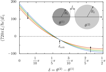
Figure 3: Lowest-order correction $E_{1}$ of the Casimir energy for PEMC spheres characterized by the material parameters $\theta^{(1)}$ and $\theta^{(2)}$ as function of $\delta=\theta^{(2)}-\theta^{(1)}$. The corrections are plotted for the sphere-sphere geometry with ratios $R_{1}/R_{2}=1$ (blue), 4 (green) and 10 (yellow) as well as for the limiting case of the plane-sphere geometry where $R_{1}/R_{2}=\infty$ (red). The direction of increasing ratios is marked by two arrows. The PFA result vanishes for $\delta_{\text{crit}}$, making the correction $E_{1}$ the leading-order term of the Casimir energy.

VI Next-to-leading order corrections for perfectly reflecting spheres at zero temperature

Finally, we will explore corrections beyond the leading ones discussed in the two previous sections. For simplicity, we will restrict ourselves to two perfectly reflecting spheres, i.e. spheres consisting of perfect electric conductors, at zero temperature. Anticipating the numerical results shown in Fig. 4, we write the asymptotic expansion of the Casimir energy as

$$E=E_{\text{PFA}}\left[1+\beta_{1}x+\beta_{3/2}x^{3/2}+\ldots\right]$$ (86)

with the aspect ratio defined in (78) and the PFA result for perfect electric conductors given in (84). As was found for $\beta_{\text{geo}}$ in (82), the coefficient $\beta_{3/2}$ may in general depend on the ratio of the sphere radii through the dimensionless quantity $u$ defined in (74).

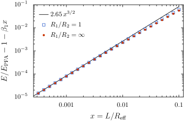
Figure 4: Numerical results for the correction to the Casimir energy beyond the linear term are shown for perfectly reflecting spheres of equal radii (open squares) and a plane-sphere setup (filled circles) at separation $L$ in vacuum at zero temperature. The solid line, representing $2.65\,x^{3/2}$, corresponds to a numerical fit on the plane-sphere results obtained in Ref. Hartmann, 2018.

In Fig. 4, numerical results for the correction beyond the linear term are shown for two spheres of equal radii (open squares) and a plane-sphere setup (filled circles). Results for spheres with different radii have been found to lie between these two data sets. The solid line represents the function $2.65\,x^{3/2}$ obtained by a numerical fit to the plane-sphere results at $x\leq 10^{-3}$ Hartmann (2018). The data for the sphere-sphere geometry appear to approach the same asymptotic behavior for the next-to-leading-order (NTLO) correction. With increasing aspect ratio $x$, the data tend to deviate from the fit because of higher order corrections.

On the basis of our considerations in previous sections, one might have expected that already the NTLO correction should be proportional to $x^{2}$. The NTLO correction to the saddle-point approximation would give rise to such a term as would the NTLO correction of the Mie scattering amplitudes $S_{\mathrm{TE},\mathrm{TE}}$ and $S_{\mathrm{TM},\mathrm{TM}}$ for perfect reflectors (cf. Fig. 7.5 on page 99 in Ref. Spreng, 2021). However, this expectation is clearly refuted by the numerical results. Our aim in the remainder of this section is thus to understand the origin of a correction proportional to $x^{3/2}$. We will refrain from trying to obtain the prefactor analytically which would require the push the evaluation of the saddle-point approximation even one order further than we did in Sec. V.2. Instead, we will show that already an appropriate evaluation of diffractive corrections will yield the observed power law.

Proceeding as in Sec. IV, one would encounter a logarithmic divergence in the round-trip sum. Instead we follow a strategy similar to the one employed in Ref. Henning et al., 2021 where the corrections to PFA were calculated in an intermediate temperature regime. For perfectly reflecting spheres, only the polarization preserving scattering amplitudes (21) are nonvanishing and the diffractive correction $s_{pp}$ is given by the first term in (23) and (24) for $p=\mathrm{TE},\mathrm{TM}$, respectively. The key ingredient for the calculation of the NTLO correction consists now in replacing $1+s_{pp}/\tilde{\xi}$ by $\exp(s_{pp}/\tilde{\xi})$ in (22) which is correct up to order $\tilde{\xi}^{-1}$. Note that the leading corrections $s_{pp}$ of the scattering amplitudes take on negative values, thus ensuring later the convergence of the round-trip sum.

This exponential replacement implies that diffractive corrections are taken into account for an arbitrary number of reflections during the round-trips. In contrast, in Sec. V.1 a diffractive correction was taken into account only at one of the reflections during the series of round-trips. Mathematically, the exponential replacement amounts to a resummation of higher-order diffractive corrections.

Applying the exponential replacement in (43), we can express the leading-order of the saddle-point approximation as

$$\left[\mathrm{tr}\mathcal{M}^{r}\right]_{\text{LO-SPA}}=\frac{R_{\mathrm{eff}}}{2r}\sum_{p}\int_{0}^{\infty}dk_{\mathrm{sp}}\frac{k_{\mathrm{sp}}}{\kappa_{\mathrm{sp}}}\exp\left[-r\left(2\kappa_{\mathrm{sp}}L-\frac{c}{\xi R_{\mathrm{eff}}}s_{pp}\right)\right]\,,$$ (87)

where it is implicitly understood that the functions $s_{pp}$ have been evaluated on the saddle-point manifold (40).

An expression for the Casimir energy can now be obtained from (87) together with (3) and (6). It is convenient to introduce a new integration variable $t=\xi/c\kappa_{\mathrm{sp}}$ to obtain

$$E_{\text{LO-SPA}}=-\frac{\hbar cR_{\mathrm{eff}}}{4\pi}\sum_{p}\int_{0}^{1}dt\sum_{r=1}^{\infty}\frac{1}{r^{2}}\int_{0}^{\infty}d\kappa_{\mathrm{sp}}\,\kappa_{\mathrm{sp}}\exp\left[-2r\left(\kappa_{\mathrm{sp}}L+\frac{1}{\kappa_{\mathrm{sp}}R_{\mathrm{eff}}}\sigma_{p}\right)\right]\,,$$ (88)

where

$$\sigma_{\mathrm{TE}} \equiv-\left.\frac{c\kappa}{2\xi}s_{\mathrm{TE},\mathrm{TE}}\right|_{\mathrm{sp}}=\frac{2-t^{2}}{4}\,,$$ (89)

$$\sigma_{\mathrm{TM}} \equiv-\left.\frac{c\kappa}{2\xi}s_{\mathrm{TM},\mathrm{TM}}\right|_{\mathrm{sp}}=\frac{t^{2}}{4}$$

are positive in the range of integration. The integration over $\kappa_{\mathrm{sp}}$ can now be carried out yielding essentially a modified Bessel function of the second kind $K_{2}(4r\sqrt{\sigma_{p}x})$.Gradshteyn and Ryzhik (1980)

We now need to find an asymptotic expansion for $x\ll 1$. Indeed an asymptotic expansion of the sum over round-trips containing the modified Bessel function can be worked out using a method from Ref. Paris, 2018. We find

$$\sum_{r=1}^{\infty}\frac{K_{2}(4r\sqrt{z})}{r^{2}}\sim\frac{\pi^{4}}{720z}-\frac{\pi^{2}}{12}+\frac{2\pi\sqrt{z}}{3}+O(z\log(z))$$ (90)

for $z\ll 1$. Evaluating finally the integral over $t$, the Casimir energy in lowest order of the saddle-point approximation, but including diffractive corrections yields

$$E_{\text{LO-SPA}} =-\frac{\hbar c\pi^{3}R_{\mathrm{eff}}}{720L^{2}}\bigg{[}1-\frac{15}{\pi^{2}}x$$ (91)

$$\qquad\qquad\qquad+\frac{15(10+3\pi)}{4\pi^{3}}x^{3/2}+\dots\bigg{]}\,.$$

As expected, this result reproduces the PFA result (84) and the leading-order correction due to diffraction as given by $\beta_{\text{diff}}$ in (82) for $\delta=0$. The NTLO correction is indeed found to go with the power 3/2 of the aspect ratio $x$ but the prefactor accounts only for about 89% of the numerical result. This discrepancy can be explained by the fact that the NTLO-SPA and NNTLO-SPA contributions have been neglected in the calculation. Since the diffractive correction is independent of $u$, only a small contribution from other corrections can depend on $u$, thus explaining the weak dependence of $\beta_{3/2}$ on $u$ found in the numerical results. Moreover, analyzing the contributions of the individual polarizations, one finds that the main contribution comes from TE polarization with about $90\%$ of the full correction.

Finally, we note that our calculation can be straightforwardly extended to real dielectric materials, implying that the appearance of the $x^{3/2}$ term in the asymptotic expansion should not be restricted to perfectly reflecting spheres. Numerical results for the plane-sphere geometry indeed show that within the Drude or the plasma model describing the metallic objects, a $x^{3/2}$-term does occur Hartmann (2018).

VII Conclusions

Plane waves can constitute a basis well suited for the study of the Casimir effect as we have shown here by reviewing recent work in this direction. They turn out to be useful for numerical as well as analytical work, in particular when the distance between the involved objects is small as is the case in most experiments. As we demonstrated, plane waves lend themselves particularly well for an interpretation in terms of geometrical optics and diffractive corrections.

For a setup consisting of two spheres with an arbitrary ratio of radii in vacuum, we have demonstrated that the proximity-force approximation can be obtained as the leading term in an asymptotic expansion for large radii. A previous calculation based on the saddle-point approximation of the trace over a given number of round-trips of electromagnetic waves between the spheres was extended to spheres made of bi-isotropic material where one needs to account for polarization mixing during the reflection processes. The result was shown to be naturally explained in terms of geometrical optics.

The framework provided by the saddle-point approximation allowed us to derive leading-order corrections, both of geometrical and diffractive origin. Explicit results were given for the first time for PEMC spheres at zero temperature. It turned out that for a suitable choice of material parameters, the contribution of the proximity-force approximation vanishes and the leading-order correction actually becomes the dominant term in the Casimir energy.

Finally, numerical results for two perfectly reflecting spheres at small values of $x=L/R_{\mathrm{eff}}$ motivated us to go one order further. We found that the next-to-leading-order correction to PFA goes as $x^{3/2}$ rather than $x^{2}.$ We discussed its origin as a resummation of higher-order diffractive corrections. The $x^{3/2}$ term implies that the estimation of the total correction to PFA based on the the linear order alone is of limited interest for practical purposes, particularly in situations where beyond-PFA results are required.

It can be expected that the usefulness of the plane-wave basis is not limited to spherical objects but that this basis has potential for a study of the Casimir interaction between a much wider class of systems.

References

- Casimir (1948) H. B. G. Casimir, Proc. Kon. Ned. Akad. Wetenschappen 51, 79 (1948).
- Klimchitskaya and Mostepanenko (2006) G. L. Klimchitskaya and V. M. Mostepanenko, Contemp. Physics. 47, 131 (2006).
- Klimchitskaya et al. (2009) G. L. Klimchitskaya, U. Mohideen, and V. M. Mostepanenko, Rev. Mod. Phys. 81, 1827 (2009).
- Decca et al. (2011) R. S. Decca, V. Aksyuk, and D. López, Casimir Force in Micro and Nano Electro Mechanical Systems (Springer, 2011), vol. 834 of Lecture Notes in Physics, pp. 287–309.
- Lamoreaux (2011) S. K. Lamoreaux, Progress in Experimental Measurements of the Surface–-Surface Casimir Force: Electrostatic Calibrations and Limitations to Accuracy (Springer, 2011), vol. 834 of Lecture Notes in Physics, pp. 219–248.
- Klimchitskaya and Mostepanenko (2020) G. L. Klimchitskaya and V. M. Mostepanenko, Mod. Phys. Lett. A 35, 2040007 (2020).
- Mostepanenko and Klimchitskaya (2020) V. M. Mostepanenko and G. L. Klimchitskaya, Universe 6, 147 (2020).
- Gong et al. (2021) T. Gong, M. R. Corrado, A. R. Mahbub, C. Shelden, and J. N. Munday, Nanophotonics 10, 523 (2021).
- Ether jr. et al. (2015) D. S. Ether jr., L. B. Pires, S. Umrath, D. Martinez, Y. Ayala, B. Pontes, G. R. de S. Araújo, S. Frases, G.-L. Ingold, F. S. S. Rosa, et al., EPL 112, 44001 (2015).
- Garrett et al. (2018) J. L. Garrett, D. A. T. Somers, and J. N. Munday, Phys. Rev. Lett. 120, 040401 (2018).
- Pires et al. (2021) L. B. Pires, D. S. Ether, B. Spreng, G. R. S. Araújo, R. S. Decca, R. S. Dutra, M. Borges, F. S. S. Rosa, G.-L. Ingold, M. J. B. Moura, et al., Phys. Rev. Res. 3, 033037 (2021).
- Hartmann et al. (2018) M. Hartmann, G.-L. Ingold, and P. A. Maia Neto, Phys. Scr. 93, 114003 (2018).
- Derjaguin (1934) B. Derjaguin, Kolloid-Z. 69, 155 (1934).
- Błocki et al. (1977) J. Błocki, J. Randrup, W. J. Świątecki, and C. F. Tsang, Ann. Phys. (N.Y.) 105, 427 (1977).
- Krause et al. (2007) D. E. Krause, R. S. Decca, D. López, and E. Fischbach, Phys. Rev. Lett. 98, 050403 (2007).
- Liu et al. (2019a) M. Liu, J. Xu, G. L. Klimchitskaya, V. M. Mostepanenko, and U. Mohideen, Phys. Rev. B 100, 081406 (2019a).
- Liu et al. (2019b) M. Liu, J. Xu, G. L. Klimchitskaya, V. M. Mostepanenko, and U. Mohideen, Phys. Rev. A 100, 052511 (2019b).
- Decca et al. (2007) R. S. Decca, D. López, E. Fischbach, G. L. Klimchitskaya, D. E. Krause, and V. M. Mostepanenko, Phys. Rev. D 75, 077101 (2007).
- Mostepanenko (2021) V. M. Mostepanenko, Universe 7, 84 (2021).
- Fosco et al. (2011) C. D. Fosco, F. C. Lombardo, and F. D. Mazzitelli, Phys. Rev. D 84, 105031 (2011).
- Fosco et al. (2014) C. D. Fosco, F. C. Lombardo, and F. D. Mazzitelli, Phys. Rev. A 89, 062120 (2014).
- Oskooi et al. (2010) A. F. Oskooi, D. Roundy, M. Ibanescu, P. Bermel, J. D. Joannopoulos, and S. G. Johnson, Comput. Phys. Commun. 181, 687 (2010).
- Reid and Johnson (2015) M. T. H. Reid and S. G. Johnson, IEEE Trans. Antennas Propag. 63, 3588 (2015).
- Hartmann and Ingold (2020) M. Hartmann and G.-L. Ingold, J. Open Source Software 5, 2011 (2020).
- Hartmann et al. (2017) M. Hartmann, G.-L. Ingold, and P. A. Maia Neto, Phys. Rev. Lett. 119, 043901 (2017).
- Bimonte and Emig (2012) G. Bimonte and T. Emig, Phys. Rev. Lett. 109, 160403 (2012).
- Spreng et al. (2020) B. Spreng, P. A. Maia Neto, and G.-L. Ingold, J. Chem. Phys. 153, 024115 (2020).
- Nunes et al. (2021) R. O. Nunes, B. Spreng, R. de Melo e Souza, G.-L. Ingold, P. A. Maia Neto, and F. S. S. Rosa, Universe 7, 156 (2021).
- Spreng (2021) B. Spreng, Ph.D. thesis, Universität Augsburg (2021), https://opus.bibliothek.uni-augsburg.de/opus4/86198.
- Bimonte et al. (2021) G. Bimonte, B. Spreng, P. A. Maia Neto, G.-L. Ingold, G. L. Klimchitskaya, V. M. Mostepanenko, and R. S. Decca, Universe 7, 93 (2021).
- (31) T. Schoger, B. Spreng, G.-L. Ingold, A. Lambrecht, P. A. Maia Neto, and S. Reynaud, to appear in Int. J. Mod. Phys. A.
- Lambrecht et al. (2006) A. Lambrecht, P. A. Maia Neto, and S. Reynaud, New J. Phys. 8, 243 (2006).
- Emig et al. (2007) T. Emig, N. Graham, R. L. Jaffe, and M. Kardar, Phys. Rev. Lett. 99, 170403 (2007).
- Ingold and Lambrecht (2015) G.-L. Ingold and A. Lambrecht, Am. J. Phys. 83, 156 (2015).
- Spreng et al. (2018) B. Spreng, M. Hartmann, V. Henning, P. A. Maia Neto, and G.-L. Ingold, Phys. Rev. A 97, 062504 (2018).
- Henning et al. (2019) V. Henning, B. Spreng, M. Hartmann, G.-L. Ingold, and P. A. Maia Neto, J. Opt. Soc. Am. B 36, C77 (2019).
- Henning et al. (2021) V. Henning, B. Spreng, P. A. Maia Neto, and G.-L. Ingold, Universe 7, 129 (2021).
- Schoger and Ingold (2021) T. Schoger and G.-L. Ingold, SciPost Phys. Core 4, 011 (2021).
- Bordag and Nikolaev (2008) M. Bordag and V. Nikolaev, J. Phys. A: Math. Theor. 41, 164002 (2008).
- Emig (2008) T. Emig, J. Stat. Mech. 2008, P04007 (2008).
- Maia Neto et al. (2008) P. A. Maia Neto, A. Lambrecht, and S. Reynaud, Phys. Rev. A 78, 012115 (2008).
- Teo et al. (2011) L. P. Teo, M. Bordag, and V. Nikolaev, Phys. Rev. D 84, 125037 (2011).
- Bimonte et al. (2012) G. Bimonte, T. Emig, R. L. Jaffe, and M. Kardar, EPL 97, 50001 (2012).
- Teo (2013) L. P. Teo, Phys. Rev. D 88, 045019 (2013).
- Canaguier-Durand et al. (2012) A. Canaguier-Durand, G.-L. Ingold, M.-T. Jaekel, A. Lambrecht, P. A. Maia Neto, and S. Reynaud, Phys. Rev. A 85, 052501 (2012).
- Teo (2012) L. P. Teo, Phys. Rev. D 85, 045027 (2012).
- Fosco et al. (2016) C. D. Fosco, F. C. Lombardo, and F. D. Mazzitelli, Phys. Rev. D 93, 125015 (2016).
- Guérout et al. (2018) R. Guérout, G.-L. Ingold, A. Lambrecht, and S. Reynaud, Symmetry 10, 37 (2018).
- Nieto-Vesperinas (2006) M. Nieto-Vesperinas, Scattering and Diffraction in Physical Optics (World Scientific, 2006), 2nd ed., eprint https://www.worldscientific.com/doi/pdf/10.1142/5833.
- Mie (1908) G. Mie, Ann. Phys. (Leipzig) 330, 377 (1908).
- van de Hulst (1981) H. C. van de Hulst, Light Scattering by Small Particles (Dover Publications, New York, 1981), ISBN 978-0-486-64228-4, chap. 12.
- Bohren and Huffman (2004) C. F. Bohren and D. R. Huffman, Absorption and Scattering of Light by Small Particles (Wiley-VCH, Weinheim, 2004), ISBN 978-0-471-29340-8, chap. 4.
- Sihvola and Lindell (1991) A. H. Sihvola and I. V. Lindell, Microwave and Opt. Tech. Lett. 4, 295 (1991).
- Condon (1937) E. U. Condon, Rev. Mod. Phys. 9, 432 (1937).
- Lindell and Sihvola (2005) I. V. Lindell and A. H. Sihvola, J. Electromagn. Waves Appl. 19, 861 (2005).
- Rode et al. (2018) S. Rode, R. Bennett, and S. Y. Buhmann, New J. Phys. 20, 043024 (2018).
- Bohren (1974) C. F. Bohren, Chem. Phys. Lett. 29, 458 (1974), ISSN 0009-2614.
- (58) DLMF, NIST Digital Library of Mathematical Functions, http://dlmf.nist.gov/, Release 1.1.4 of 2022-01-15, f. W. J. Olver, A. B. Olde Daalhuis, D. W. Lozier, B. I. Schneider, R. F. Boisvert, C. W. Clark, B. R. Miller, B. V. Saunders, H. S. Cohl, and M. A. McClain, eds., URL http://dlmf.nist.gov/.
- Mishchenko (2000) M. I. Mishchenko, Appl. Opt. 39, 1026 (2000).
- Messina et al. (2015) R. Messina, P. A. Maia Neto, B. Guizal, and M. Antezza, Phys. Rev. A 92, 062504 (2015).
- Nussenzveig (1969) H. M. Nussenzveig, J. Math. Phys. 10, 82 (1969).
- Nussenzveig (1992) H. M. Nussenzveig, Diffraction Effects in Semiclassical Scattering (Cambridge University Press, Cambridge, 1992), ISBN 0-521-38318-8.
- Grandy Jr (2000) W. T. Grandy Jr, Scattering of Waves from Large Spheres (Cambridge University Press, Cambridge, 2000), ISBN 978-0-521-66126-3.
- Lindell et al. (1994) I. V. Lindell, A. H. Sihvola, S. Tretyakov, and A. Viitanen, Electromagnetic waves in chiral and bi-isotropic media (Artech House, Norwood, 1994), ISBN 0890066841.
- Khare (1975) V. Khare, Ph.D. thesis, University of Rochester (1975).
- Ruppin (2006) R. Ruppin, J. Electromagn. Waves Appl. 20, 1569 (2006).
- (67) T. Schoger, unpublished.
- Jonquière (1889) A. Jonquière, Bull. de la Soc. Math. de France 17, 142 (1889).
- Boyer (1974) T. H. Boyer, Phys. Rev. A 9, 2078 (1974).
- Asorey and Muñoz-Castañeda (2013) M. Asorey and J. M. Muñoz-Castañeda, Attractive and repulsive casimir vacuum energy with general boundary conditions (2013).
- Hartmann (2018) M. Hartmann, Ph.D. thesis, Universität Augsburg (2018), https://opus.bibliothek.uni-augsburg.de/opus4/44798.
- Gradshteyn and Ryzhik (1980) I. S. Gradshteyn and I. M. Ryzhik, Table of Integrals, Series, and Products (Academic Press, New York, 1980), ISBN 0-12-294760-6.
- Paris (2018) R. B. Paris, Math. Æterna 8, 71 (2018).