Abstract

The exact solution of the $D^{(1)}_{2}$ quantum spin chain with generic non-diagonal boundary reflections is obtained. It is found that the generating functional of conserved quantities of the system can be factorized as the product of transfer matrices of two anisotropic $XXZ$ spin chains with open boundary conditions. By using the factorization identities and the fusion technique, the eigenvalues and the Bethe ansatz equations of the model are obtained. The eigenvalues are also parameterized by the zero roots of the transfer matrix, and the patterns of root distributions are obtained. Based on them, ground states energy and the surface energies induced by the twisted boundary magnetic fields in the thermodynamic limit are obtained. These results are checked by the numerical calculations. The corresponding isotropic limit is also discussed. The results given in this paper are the foundation to study the exact physical properties of high rank $D^{(1)}_{n}$ model by using the nested processes.

PACS: 75.10.Pq, 02.30.Ik, 71.10.Pm

Keywords: Bethe Ansatz; Lattice Integrable Models; Quantum Integrable Systems

1 Introduction

The $D^{(1)}_{2}$ spin chain is a typical one-dimensional quantum integrable system and has many applications in the high energy, topological and mathematical physics. The corresponding exact solution is the foundation to exactly solve the high rank $D^{(1)}_{n}$ spin chain by the nested methods. Each spin of the $D^{(1)}_{2}$ chain has four components thus the integrable $D^{(1)}_{2}$ model is characterized by the $16\times 16$ $R$-matrix [1, 2, 3], which is the solution of Yang-Baxter equation. Staring from the $R$-matrix, the transfer matrix and conserved quantities including the Hamiltonian of the system with periodic boundary condition can be constructed by using the quantum inverse scattering method. Eigenvalues of the transfer matrix of the periodic $D^{(1)}_{n}$ model are obtained by using the analytical Bethe ansatz [4, 5] and then by the algebraic Bethe ansatz [6].

Later, it was found that the $D^{(1)}_{2}$ spin chain with certain open boundary conditions can also be solved exactly, where the boundary reflections are quantified by the reflection matrices which are the solutions of reflection equations [7, 8, 9]. For the open boundary case, the conserved quantities are generated by the transfer matrix consisted of the $R$-matrices and reflection matrices [10, 11, 12]. If the boundary reflection matrices only have the diagonal elements, the particle numbers of each spin-component are conserved. In this case, the quasi-vacuum (or the reference) state is easy to be constructed, and the eigenvalues and Bethe-type eigenstates of the transfer matrix and Bethe ansatz equations can be obtained by the nested algebraic Bethe ansatz [13, 14, 15, 16, 17]. Then based on the Bethe states, the correlation function, norm, form factor and other scalar products can be calculated. The interesting thing is that how to diagonalize the transfer matrix if the reflection matrices are non-diagonal. Due to the fact that the reflection matrices at the two ends can not be diagonalized simultaneously, the $U(1)$ symmetry of the system is broken. Then the traditional nested algebraic Bethe ansatz does not work.

Recently, in an interesting work [18], Robertson, Pawelkiewicz, Jacobsen and Saleur showed that the $R$-matrix of the $D^{(2)}_{2}$ model is related with the antiferromagnetic Potts model and the staggered $XXZ$ spin chain [19, 20, 21, 22, 23, 24, 25]. It opens a new way to diagonalize the integrable model beyond the $A$-series Lie algebra. Based on this idea and using the algebraic Bethe ansatz, Nepomechie and Retore obtained the exact solution of both the closed and open $D^{(2)}_{2}$ spin chains [26].

In this paper, we study the exact solution of the $D^{(1)}_{2}$ spin chain with non-diagonal boundary reflections. We find that the transfer matrix of the model can be factorized as the product of transfer matrices of two six-vertex models with generic integrable open boundary condition. With the help of this factorization identity and using the fusion, we obtain the eigenvalues expressed by the inhomogeneous $T-Q$ relation and the Bethe ansatz equations of the model. In order to study the physical properties of the system, we also use the $t-W$ scheme and obtain the patterns of zero roots distributions. Based on them, we obtain the ground state energy and the surface energy induced by the non-diagonal boundary magnetic fields in the thermodynamic limit and check these results numerically. The results of both the anisotropic and isotropic $D^{(1)}_{2}$ spin chains are given.

This paper is organized as follows. In section 2, we give a brief description of the anisotropic $D^{(1)}_{2}$ spin chain with open boundaries. The $R$-matrix, reflection matrices and generating functional of conserved quantities are introduced. In section 3, we show that the transfer matrix can be factorized as the product of two $XXZ$ spin chains. In section 4, by using the fusion technique, we calculate the exact solution of the system. The inhomogeneous $T-Q$ relation and related Bethe ansatz equations are given. In section 5, the thermodynamic limit and the surface energies of the anisotropic $D^{(1)}_{2}$ spin chain are studied. In section 6, we list the results of the isotropic $D^{(1)}_{2}$ spin chain. The summary of main results and some concluding remarks are presented in section 7.

2 Anisotropic $D^{(1)}_{2}$ spin chain

Each spin in the $D^{(1)}_{2}$ model has four components. The anisotropic spin-exchanging interaction is quantified by the $4^{2}\times 4^{2}$ $R$-matrix [1, 2, 3]

$$R_{12}(u)=\left(\begin{array}[]{cccc|cccc|cccc|cccc}a&&&&&&&&&&&&&&&\\ &b&&&g_{1}&&&&&&&&&&&\\ &&b&&&&&&g_{1}&&&&&&&\\ &&&e&&&d_{1}&&&d_{1}&&&c_{1}&&&\\ \hline\cr&{g}_{2}&&&b&&&&&&&&&&&\\ &&&&&a&&&&&&&&&&\\ &&&{d}_{2}&&&e&&&{c}&&&d_{1}&&&\\ &&&&&&&b&&&&&&g_{1}&&\\ \hline\cr&&{g}_{2}&&&&&&b&&&&&&&\\ &&&{d}_{2}&&&{c}&&&e&&&d_{1}&&&\\ &&&&&&&&&&a&&&&&\\ &&&&&&&&&&&b&&&g_{1}&\\ \hline\cr&&&{c}_{2}&&&{d}_{2}&&&{d_{2}}&&&e&&&\\ &&&&&&&{g}_{2}&&&&&&b&&\\ &&&&&&&&&&&{g_{2}}&&&b&\\ &&&&&&&&&&&&&&&a\\ \end{array}\right),$$ (2.17)

where $u$ is the spectral parameter, the non-zero matrix elements are

$$a=2\sinh^{2}(\frac{u}{2}-2\eta),\;\;\;b=2\sinh\frac{u}{2}\sinh(\frac{u}{2}-2\eta),\;\;\;e=2\sinh^{2}\frac{u}{2},\;\;\;c=2\sinh^{2}(2\eta),$$

$$g_{1}=-2e^{-\frac{u}{2}}\sinh(2\eta)\sinh(\frac{u}{2}-2\eta),\;\;\;g_{2}=e^{u}g_{1},\;\;\;d_{1}=2e^{-\frac{u}{2}}\sinh\frac{u}{2}\sinh(2\eta),$$

$$d_{2}=e^{u}d_{1},\;\;\;c_{1}=2e^{-u}\sinh^{2}(2\eta),\;\;\;c_{2}=2e^{u}\sinh^{2}(2\eta),$$ (2.18)

and $\eta$ is the crossing or anisotropic parameter. The $R$-matrix (2.17) is defined in the tensor space $V_{1}\otimes V_{2}$, where $V_{1}$ and $V_{2}$ are two four-dimensional linear spaces, and has the properties

$${\rm Periodicity} : R_{12}(u+2i\pi)=R_{12}(u),$$

$${\rm PT-symmetry} : R^{t_{1}t_{2}}_{12}(u)=R_{12}(u),$$

$${\rm Unitarity} : R_{12}(u)R_{21}(-u)=\rho(u)=4\sinh^{2}(\frac{u}{2}-2\eta)\sinh^{2}(\frac{u}{2}+2\eta),$$

$${\rm Initial\,\,condition} : R_{12}(0)=\rho(0)^{\frac{1}{2}}P_{12},$$

$${\rm Crossing\,\,unitarity} : R_{12}(u)^{t_{1}}{M}_{1}R_{21}(-u+8\eta)^{t_{1}}{M}_{1}^{-1}=\rho(u-4\eta),$$ (2.19)

where ${P}_{12}$ is the permutation operator with the matrix elements $[{P}_{12}]^{\alpha\gamma}_{\beta\delta}=\delta_{\alpha\delta}\delta_{\beta\gamma}$, $R_{21}(u)={P}_{12}R_{12}(u){P}_{12}$, $t_{1}$ (or $t_{2}$) denotes the transposition in the subspace $V_{1}$ (or $V_{2}$) and $M_{1}$ is the $4\times 4$ diagonal constant matrix defined in the space $V_{1}$

$${M}_{1}=M=diag(e^{4\eta},1,1,e^{-4\eta}).$$ (2.20)

Besides, the $R$-matrix (2.17) satisfies the Yang-Baxter equation

$$R_{12}(u-v)R_{13}(u)R_{23}(v)=R_{23}(v)R_{13}(u)R_{12}(u-v),$$ (2.21)

which means that the scattering processes among the quasi-particle do not depend on the paths.

The boundary reflection at one end is characterized by the reflection matrix

$$K(u)=\left(\begin{array}[]{cccc}k_{11}(u)&k_{12}(u)&k_{13}(u)&k_{14}(u)\\ k_{21}(u)&k_{22}(u)&k_{23}(u)&k_{24}(u)\\ k_{31}(u)&k_{32}(u)&k_{33}(u)&k_{34}(u)\\ k_{41}(u)&k_{42}(u)&k_{43}(u)&k_{44}(u)\end{array}\right),$$ (2.26)

where matrix elements are

$$k_{11}(u)=e^{-u}\sinh(s-\frac{u}{2})\sinh(t-\frac{u}{2}),\quad k_{12}(u)=-e^{-\frac{u}{2}}t_{1}\sinh(s-\frac{u}{2})\sinh u,$$

$$k_{13}(u)=e^{-\frac{u}{2}}s_{1}\sinh(t-\frac{u}{2})\sinh u,\quad k_{14}(u)=s_{1}t_{1}\sinh^{2}u,$$

$$k_{21}(u)=-e^{-\frac{u}{2}}t_{2}\sinh(s-\frac{u}{2})\sinh u,\quad k_{22}(u)=\sinh(s-\frac{u}{2})\sinh(t+\frac{u}{2}),$$

$$k_{23}(u)=-s_{1}t_{2}\sinh^{2}u,\quad k_{24}(u)=-e^{\frac{u}{2}}s_{1}\sinh(t+\frac{u}{2})\sinh u,$$

$$k_{31}(u)=e^{-\frac{u}{2}}s_{2}\sinh(t-\frac{u}{2})\sinh u,\quad k_{32}(u)=-s_{2}t_{1}\sinh^{2}u,$$

$$k_{33}(u)=\sinh(s+\frac{u}{2})\sinh(t-\frac{u}{2}),\quad k_{34}(u)=e^{\frac{u}{2}}t_{1}\sinh(s+\frac{u}{2})\sinh u,$$

$$k_{41}(u)=s_{2}t_{2}\sinh^{2}u,\quad k_{42}(u)=-e^{\frac{u}{2}}s_{2}\sinh(t+\frac{u}{2})\sinh u,$$

$$k_{43}(u)=e^{\frac{u}{2}}t_{2}\sinh(s+\frac{u}{2})\sinh u,\quad k_{44}(u)=e^{u}\sinh(s+\frac{u}{2})\sinh(t+\frac{u}{2}),$$ (2.27)

and $\{t,t_{1},t_{2},s,s_{1},s_{2}\}$ are six free boundary parameters. The reflection matrix (2.26) satisfies the reflection equation [10, 11]

$$R_{12}(u-v){K_{1}}(u)R_{21}(u+v){K_{2}}(v)={K_{2}}(v)R_{12}(u+v){K_{1}}(u)R_{21}(u-v),$$ (2.28)

where $K_{1}(u)=K(u)\otimes I$, $K_{2}(u)=I\otimes K(u)$ and $I$ is the $4\times 4$ unit matrix. The boundary reflection at the other end is quantified by the dual reflection matrix

$$\bar{K}(u)=MK(-u+4\eta)|_{\{t,t_{1},t_{2},s,s_{1},s_{2}\}\rightarrow\{t^{\prime},t^{\prime}_{1},t^{\prime}_{2},s^{\prime},s^{\prime}_{1},s^{\prime}_{2}\}},$$ (2.29)

where $\{t^{\prime},t^{\prime}_{1},$ $t^{\prime}_{2},s^{\prime},s^{\prime}_{1},s^{\prime}_{2}\}$ are the free boundary parameters. The dual reflection matrix (2.29) satisfies the dual reflection equation [10, 11, 12]

$$R_{12}(-u+v){\bar{K}_{1}}(u)M_{1}^{-1}R_{21}(-u-v+8\eta)M_{1}{\bar{K}_{2}}(v)$$

$$\qquad={\bar{K}_{2}}(v)M_{1}R_{12}(-u-v+8\eta)M_{1}^{-1}\bar{K}_{1}(u)R_{21}(-u+v),$$ (2.30)

where $\bar{K}_{1}(u)=\bar{K}(u)\otimes I$ and $\bar{K}_{2}(u)=I\otimes\bar{K}(u)$.

Now, we are ready to construct the quantum many-body system with interactions. The conserved quantities including the model Hamiltonian of $D_{2}^{(1)}$ spin chain is generated by the transfer matrix $t(u)$

$$t(u)=tr_{0}\{\bar{K}_{0}(u)T_{0}(u)K_{0}(u)\hat{T}_{0}(u)\}.$$ (2.31)

Here the subscript $0$ means the four-dimensional auxiliary space $V_{0}$ and $tr_{0}$ means taking trace only in the auxiliary space. $T_{0}(u)$ and $\hat{T}_{0}(u)$ are the monodromy matrix and the reflecting one, respectively,

$$T_{0}(u)=R_{01}(u-\theta_{1})R_{02}(u-\theta_{2})\cdots R_{0N}(u-\theta_{N}),$$

$$\hat{T}_{0}(u)=R_{N0}(u+\theta_{N})\cdots R_{20}(u+\theta_{2})R_{10}(u+\theta_{1}),$$ (2.32)

where $\{\theta_{j}|j=1,\cdots,N\}$ are the inhomogeneity parameters and $N$ is the number of sites. $T_{0}(u)$ and $\hat{T}_{0}(u)$ are defined in the tensor space $V_{0}\otimes V_{q}$ and $V_{q}=\otimes_{j=1}^{N}V_{j}$ is the physical space. From the Yang-Baxter relation (2.21), reflection equation (2.28) and the dual one (2.30), we can prove that the transfer matrices with different spectral parameters commutate with each other

$$[t(u),t(v)]=0.$$ (2.33)

Thus the system is integrable. Expanding $t(u)$ with respect to $u$, all the coefficients and their combinations are the conserved quantities. The model Hamiltonian of the integrable $D^{(1)}_{2}$ quantum spin chain is obtained by taking the derivative of logarithm of the transfer matrix $t(u)$ with the homogeneous limit $\{\theta_{j}\}=0$

$$H = \frac{\partial\ln t(u)}{2\partial u}|_{u=0,\{\theta_{j}\}=0}-\frac{tr_{0}{\bar{K}_{0}}(0)^{\prime}}{2tr_{0}\bar{K}_{0}(0)}$$ (2.34)

$$= \sum^{N-1}_{k=1}H_{kk+1}+\frac{{K_{N}}(0)^{\prime}}{2{K_{N}}(0)}+\frac{tr_{0}\{\bar{K}_{0}(0)H_{10}\}}{tr_{0}\bar{K}_{0}(0)},$$

where $H_{k\,k+1}=\rho^{-1}(0){R}_{k\,k+1}(0)\,\frac{\partial}{\partial u}R_{k\,k+1}(u)\left.\right|_{u=0}$ and $H_{10}=P_{01}H_{01}P_{01}$.

The next task is to diagonalize the transfer matrix $t(u)$. However, the reflection matrices $K(u)$ and $\bar{K}(u)$ have the non-diagonal elements and can not be diagonalized simultaneously. It is very hard to construct the reference state and to solve the eigen-equation of $t(u)$ [27].

3 Factorizations

In order to obtain the eigenvalues of the transfer matrix (2.31), here we adopt the factorization method [18, 26]. The four-dimensional space can be regarded as the tensor of two equivalent two-dimensional subspaces. For example, $V_{1}=V_{1^{\prime}}\otimes V_{1^{\prime\prime}}$ and $V_{2}=V_{2^{\prime}}\otimes V_{2^{\prime\prime}}$, where the structures of $V_{1^{\prime}}$ and $V_{1^{\prime\prime}}$ are the same. Then the $R$-matrix (2.17) can be decomposed into

$$R_{12}(u)=2[S\otimes S][R^{s}_{1^{\prime}2^{\prime}}(u)\otimes R^{s}_{1^{\prime\prime}2^{\prime\prime}}(u)][S\otimes S]^{-1},$$ (3.1)

where $S$ is a $4\times 4$ diagonal constant matrix

$$S=diag(1,-1,1,1),$$ (3.2)

and $R^{s}_{1^{\prime}2^{\prime}}(u)$ is the $R$-matrix of anisotropic $XXZ$ spin chain

$$R^{s}_{1^{\prime}2^{\prime}}(u)=\left(\begin{array}[]{cccc}\sinh(\frac{u}{2}-2\eta)&&&\\ &\sinh\frac{u}{2}&-e^{-\frac{u}{2}}\sinh(2\eta)&\\ &-e^{\frac{u}{2}}\sinh(2\eta)&\sinh\frac{u}{2}&\\ &&&\sinh(\frac{u}{2}-2\eta)\\ \end{array}\right).$$ (3.7)

We shall note that the spaces of two $R$-matrices in the factorization (3.1) are different. The $R$-matrix (3.7) has following properties

$${\rm Quasi-periodicity} : R^{s}_{1^{\prime}2^{\prime}}(u+2i\pi)=-R^{s}_{1^{\prime}2^{\prime}}(u),$$

$${\rm PT-symmetry} : R^{s}_{1^{\prime}2^{\prime}}(u)^{t_{1^{\prime}}t_{2^{\prime}}}=R^{s}_{1^{\prime}2^{\prime}}(u),$$

$${\rm Unitarity} : R^{s}_{1^{\prime}2^{\prime}}(u)R^{s}_{2^{\prime}1^{\prime}}(-u)=\rho_{s}(u)=\sinh(-\frac{u}{2}+2\eta)\sinh(\frac{u}{2}+2\eta),$$

$${\rm Initial\,\,condition} : R^{s}_{1^{\prime}2^{\prime}}(0)=-\sinh(2\eta)P_{1^{\prime}2^{\prime}},$$

$${\rm Crossing\,\,unitarity} : R^{s}_{1^{\prime}2^{\prime}}(u)^{t_{1^{\prime}}}\bar{M}_{1^{\prime}}R^{s}_{2^{\prime}1^{\prime}}(-u+8\eta)^{t_{1^{\prime}}}\bar{M}_{1^{\prime}}^{-1}=\rho_{s}(u-4\eta),$$ (3.8)

where $P_{1^{\prime}2^{\prime}}$ is the $4\times 4$ permutation operator, $t_{1^{\prime}}$ and $t_{2^{\prime}}$ denote the transpositions in the subspaces $V_{1^{\prime}}$ and $V_{2^{\prime}}$, respectively, and $\bar{M}_{1^{\prime}}$ is a $2\times 2$ diagonal constant matrix $\bar{M}_{1^{\prime}}=\bar{M}=diag(e^{2\eta},e^{-2\eta})$. The $R$-matrix (3.7) satisfies Yang-Baxter equation

$$R^{s}_{1^{\prime}2^{\prime}}(u-v)R^{s}_{1^{\prime}3^{\prime}}(u)R^{s}_{2^{\prime}3^{\prime}}(v)=R^{s}_{2^{\prime}3^{\prime}}(v)R^{s}_{1^{\prime}3^{\prime}}(u)R^{s}_{1^{\prime}2^{\prime}}(u-v).$$ (3.9)

Following the same idea, the reflection matrices can be decomposed into

$$K(u)=S[K^{s+}(u)\otimes K^{s-}(u)]S^{-1},$$ (3.10)

$$\bar{K}(u)=S[\bar{K}^{s+}(u)\otimes\bar{K}^{s-}(u)]S^{-1},$$ (3.11)

where $K^{s\pm}(u)$ and $\bar{K}^{s\pm}(u)$ are the general reflection matrices of $XXZ$ spin chain

$$K^{s+}(u)=\left(\begin{array}[]{cc}-e^{-\frac{u}{2}}\sinh(\frac{u}{2}-s)&s_{1}\sinh u\\ s_{2}\sinh u&e^{\frac{u}{2}}\sinh(\frac{u}{2}+s)\end{array}\right),$$ (3.14)

$$K^{s-}(u)=K^{s+}(u)|_{\{s,s_{1},s_{2}\}\rightarrow\{t,t_{1},t_{2}\}},$$

$$\bar{K}^{s+}(u)=\bar{M}K^{s+}(-u+4\eta)|_{\{s,s_{1},s_{2}\}\rightarrow\{s^{\prime},s^{\prime}_{1},s^{\prime}_{2}\}},$$

$$\bar{K}^{s-}(u)=\bar{M}K^{s-}(-u+4\eta)|_{\{t,t_{1},t_{2}\}\rightarrow\{t^{\prime},t^{\prime}_{1},t^{\prime}_{2}\}},$$ (3.15)

which satisfy the reflection equations

$$R^{s}_{1^{\prime}2^{\prime}}(u-v){K^{s\pm}_{1^{\prime}}}(u)R^{s}_{2^{\prime}1^{\prime}}(u+v){K^{s\pm}_{2^{\prime}}}(v)={K^{s\pm}_{2^{\prime}}}(v)R^{s}_{1^{\prime}2^{\prime}}(u+v)K^{s\pm}_{1^{\prime}}(u)R^{s}_{2^{\prime}1^{\prime}}(u-v),$$

$$R^{s}_{1^{\prime}2^{\prime}}(-u+v){\bar{K}^{s\pm}_{1^{\prime}}}(u)\bar{M}_{1^{\prime}}^{-1}R^{s\pm}_{2^{\prime}1^{\prime}}(-u-v+8\eta)\bar{M}_{1^{\prime}}{\bar{K}^{s\pm}_{2^{\prime}}}(v)$$

$$\qquad\qquad\qquad\qquad={\bar{K}^{s\pm}_{2^{\prime}}}(v)\bar{M}_{1^{\prime}}R^{s}_{1^{\prime}2^{\prime}}(-u-v+8\eta)\bar{M}_{1^{\prime}}^{-1}{{\bar{K}^{s\pm}}_{1^{\prime}}}(u)R^{s}_{2^{\prime}1^{\prime}}(-u+v).$$ (3.16)

Here ${K^{s\pm}_{1^{\prime}}}(u)=K^{s\pm}(u)\otimes I^{\prime}$, ${K^{s\pm}_{2^{\prime}}}(u)=I^{\prime}\otimes K^{s\pm}(u)$, $\bar{K}^{s\pm}_{1^{\prime}}(u)=\bar{K}^{s\pm}(u)\otimes I^{\prime}$, $\bar{K}^{s\pm}_{2^{\prime}}(u)=I^{\prime}\otimes\bar{K}^{s\pm}(u)$ and $I^{\prime}$ is the $2\times 2$ unit matrix.

By using the factorizations (3.1) and (3.11), we find that the transfer matrix of $D^{(1)}_{2}$ spin chain can be factorized as the product of transfer matrices of two independent $XXZ$ spin chains

$$t(u)=4^{N}{\cal S}\,t^{s+}(u)\otimes{t}^{s-}(u)\,{\cal S}^{-1},$$ (3.17)

where ${\cal{S}}=\otimes^{N}S$ and $t^{s\pm}(u)$ are defined as

$$t^{s\pm}(u)=tr_{0^{\prime}}\{\bar{K}^{s\pm}_{0^{\prime}}(u)T^{s}_{0^{\prime}}(u)K^{s\pm}_{0^{\prime}}(u)\hat{T}^{s}_{0^{\prime}}(u)\}.$$ (3.18)

We should note that the physical spaces of $t^{s+}(u)$ and $t^{s-}(u)$ in Eq.(3.18) are different, which means that they are two independent operators, and their tensor consists the physical space of the $D^{(1)}_{2}$ spin chain. The monodromy matrix $T^{s}_{0^{\prime}}$ and reflecting one $\hat{T}^{s}_{0^{\prime}}(u)$

$$T^{s}_{0^{\prime}}(u)=R^{s}_{0^{\prime}1^{\prime}}(u-\theta_{1})R^{s}_{0^{\prime}2^{\prime}}(u-\theta_{2})\cdots R^{s}_{0^{\prime}N^{\prime}}(u-\theta_{N}),$$

$$\hat{T}^{s}_{0^{\prime}}(u)=R^{s}_{N^{\prime}0^{\prime}}(u+\theta_{N})R^{s}_{N^{\prime}-1\,0^{\prime}}(u+\theta_{N-1})\cdots R^{s}_{1^{\prime}0^{\prime}}(u+\theta_{1}),$$ (3.19)

satisfy the Yang-Baxter relations

$$R_{0^{\prime}0^{\prime\prime}}^{s}(u-v)T^{s}_{0^{\prime}}(u)T^{s}_{0^{\prime\prime}}(v)=T^{s}_{0^{\prime\prime}}(v)T^{s}_{0^{\prime}}(u)R^{s}_{0^{\prime}0^{\prime\prime}}(u-v),$$

$$R_{0^{\prime\prime}0^{\prime}}^{s}(u-v)\hat{T}^{s}_{0^{\prime}}(u)\hat{T}^{s}_{0^{\prime\prime}}(v)=\hat{T}^{s}_{0^{\prime\prime}}(v)\hat{T}^{s}_{0^{\prime\prime}}(u)R^{s}_{0^{\prime\prime}0^{\prime}}(u-v).$$ (3.20)

By using the Yang-Baxter relation (3.20) and reflection equations (3.16), we have

$$[t^{s+}(u),t^{s+}(v)]=0,\quad[t^{s-}(u),t^{s-}(v)]=0.$$ (3.21)

4 Exact solution

The transfer matrices $t^{s+}(u)$ and $t^{s-}(u)$ can be diagonalized separately. We first consider $t^{s+}(u)$. Following the method developed in [27], we adopt the fusion technique [28, 29, 30, 31, 32, 33] to diagonalize the transfer matrix $t(u)$ given by (2.31). The $R$-matrix (3.7) at the point of $u=4\eta$ degenerates into

$$R^{s}_{1^{\prime}2^{\prime}}(4\eta)=P^{(1)}_{1^{\prime}2^{\prime}}S_{1^{\prime}2^{\prime}}^{(1)},$$ (4.1)

where $S_{1^{\prime}2^{\prime}}^{(1)}$ is an irrelevant constant matrix omitted here, $P^{(1)}_{1^{\prime}2^{\prime}}$ is the one-dimensional projector operator

$$P^{(1)}_{1^{\prime}2^{\prime}}=|\psi_{0}\rangle\langle\psi_{0}|,\quad|\psi_{0}\rangle=\frac{1}{\sqrt{2\cosh\eta}}(e^{-\eta}|1^{\prime}2^{\prime}\rangle-e^{\eta}|2^{\prime}1^{\prime}\rangle),$$ (4.2)

and $\{|1^{\prime}\rangle,|2^{\prime}\rangle\}$ are the orthogonal bases of $2$-dimensional linear space $V_{1^{\prime}}$ (and $V_{2^{\prime}}$). Taking the fusion among the $R$-matrices, we obtain

$$P^{(1)}_{2^{\prime}1^{\prime}}R^{s}_{1^{\prime}3^{\prime}}(u)R^{s}_{2^{\prime}3^{\prime}}(u+4\eta)P^{(1)}_{2^{\prime}1^{\prime}}=\sinh(\frac{u}{2}+2\eta)\sinh(\frac{u}{2}-2\eta),$$

$$P^{(1)}_{1^{\prime}2^{\prime}}R^{s}_{3^{\prime}1^{\prime}}(u)R^{s}_{3^{\prime}2^{\prime}}(u+4\eta)P^{(1)}_{1^{\prime}2^{\prime}}=\sinh(\frac{u}{2}+2\eta)\sinh(\frac{u}{2}-2\eta).$$ (4.3)

The fusion of reflection matrices gives

$$P_{2^{\prime}1^{\prime}}^{(1)}K_{1^{\prime}}^{s+}(u)R^{s}_{2^{\prime}1^{\prime}}(2u+4\eta)K_{2^{\prime}}^{s+}(u+4\eta)P_{1^{\prime}2^{\prime}}^{(1)}$$

$$\quad\quad\qquad\qquad=-2\sinh(u+4\eta)\frac{1}{\alpha}\cosh\frac{u+\alpha_{1}}{2}\cosh\frac{u-\alpha_{1}}{2}\cosh\frac{u+\alpha_{2}}{2}\cosh\frac{u-\alpha_{2}}{2},$$

$$P_{1^{\prime}2^{\prime}}^{(1)}\bar{{K}}_{2^{\prime}}^{s+}(u+4\eta)M_{1^{\prime}}R^{s}_{1^{\prime}2^{\prime}}(-2u+4\eta)M_{1^{\prime}}^{-1}\bar{{K}}_{1^{\prime}}^{s+}(u)P_{2^{\prime}1^{\prime}}^{\rm(1)}$$

$$\quad\quad\qquad\qquad=2\sinh(u-4\eta)\frac{1}{\alpha^{\prime}}\cosh\frac{u+\alpha^{\prime}_{1}}{2}\cosh\frac{u-\alpha^{\prime}_{1}}{2}\cosh\frac{u+\alpha^{\prime}_{2}}{2}\cosh\frac{u-\alpha^{\prime}_{2}}{2},$$ (4.4)

where the related constants are defined as

$$\alpha=\frac{1}{2s_{1}s_{2}},\quad\cosh\alpha_{1}=\frac{\alpha}{2}+\beta,\quad\cosh\alpha_{2}=\frac{\alpha}{2}-\beta,\quad\beta=\sqrt{1+\frac{\alpha^{2}}{4}+\alpha\cosh(2s)},$$

$$\alpha^{\prime}=\frac{1}{2s^{\prime}_{1}s^{\prime}_{2}},\,\,\cosh\alpha^{\prime}_{1}=\frac{\alpha^{\prime}}{2}+\beta^{\prime},\,\,\cosh\alpha^{\prime}_{2}=\frac{\alpha^{\prime}}{2}-\beta^{\prime},\quad\beta^{\prime}=\sqrt{1+\frac{\alpha^{\prime 2}}{4}+\alpha^{\prime}\cosh(2s^{\prime})}.$$ (4.5)

Yang-Baxter relations (3.20) at certain points gives

$${T}^{s}_{0^{\prime}}(\theta_{j}){T}_{0^{\prime\prime}}^{s}(\theta_{j}+4\eta)=P^{(1)}_{0^{\prime\prime}0^{\prime}}{T}^{s}_{0^{\prime}}(\theta_{j}){T}_{0^{\prime\prime}}^{s}(\theta_{j}+4\eta),$$

$$\hat{T}^{s}_{0^{\prime}}(-\theta_{j})\hat{T}^{s}_{0^{\prime\prime}}(-\theta_{j}+4\eta)=P^{(1)}_{0^{\prime}0^{\prime\prime}}\hat{T}^{s}_{0^{\prime}}(-\theta_{j})\hat{T}^{s}_{0^{\prime\prime}}(-\theta_{j}+4\eta).$$ (4.6)

By using the fusion relations (4.3)-(4.6), we obtain

$$t^{s+}(\pm\theta_{j})\,t^{s+}(\pm\theta_{j}+4\eta)=\frac{4\sinh(\pm{\theta_{j}}-4\eta)\sinh(\pm{\theta_{j}}+4\eta)}{\alpha\alpha^{\prime}\sinh(\pm\theta_{j}-2\eta)\sinh(\pm\theta_{j}+2\eta)}\cosh\frac{\pm\theta_{j}-\alpha_{1}}{2}$$

$$\qquad\qquad\times\cosh\frac{\pm\theta_{j}+\alpha_{1}}{2}\cosh\frac{\pm\theta_{j}-\alpha_{2}}{2}\cosh\frac{\pm\theta_{j}+\alpha_{2}}{2}\cosh\frac{\pm\theta_{j}-\alpha^{\prime}_{1}}{2}\cosh\frac{\pm\theta_{j}+\alpha^{\prime}_{1}}{2}$$

$$\qquad\qquad\times\cosh\frac{\pm\theta_{j}-\alpha^{\prime}_{2}}{2}\cosh\frac{\pm\theta_{j}+\alpha^{\prime}_{2}}{2}\prod_{k=1}^{N}\sinh\frac{\pm\theta_{j}-\theta_{k}-4\eta}{2}$$

$$\qquad\qquad\times\sinh\frac{\pm\theta_{j}-\theta_{k}+4\eta}{2}\sinh\frac{\pm\theta_{j}+\theta_{k}-4\eta}{2}\sinh\frac{\pm\theta_{j}+\theta_{k}+4\eta}{2},\;j=1,\cdots,N.$$ (4.7)

Besides, the values of $t^{s+}(u)$ at the points of $u=0,4\eta,i\pi$ can be calculated directly

$$t^{s+}(0)=t^{s+}(4\eta)=2\cosh(2\eta)\sinh s\sinh s^{\prime}\prod_{j=1}^{N}\rho_{s}(\theta_{j}),$$ (4.8)

$$t^{s+}(i\pi)=t^{s+}(-i\pi+4\eta)=2\cosh(2\eta)\cosh s\cosh s^{\prime}\prod_{j=1}^{N}\rho_{s}(\theta_{j}+i\pi).$$ (4.9)

The asymptotic behavior of $t^{s+}(u)$ is

$$t^{s+}(u)|_{u\rightarrow\pm\infty}=-2^{-(2N+2)}e^{\pm[(N+2)u-2(N+2)\eta]}(e^{-2\eta}s_{1}s^{\prime}_{2}+e^{2\eta}s_{2}s^{\prime}_{1}).$$ (4.10)

From the definition, we know that the transfer matrix $t^{s+}(u)$ is an operator polynomial of $e^{\frac{u}{2}}$ with the degree $2N+4$, which can be completely determined by $2N+5$ constraints. Thus above $2N$ fusion identities (4.7) and $6$ additional conditions (4.9)-(4.10) give us sufficient information to determine the eigenvalue $\Lambda^{s+}(u)$ of $t^{s+}(u)$. After some algebra, we express the eigenvalue $\Lambda^{s+}(u)$ as the inhomogeneous $T-Q$ relation

$$\Lambda^{s+}(u)=\frac{2\sinh(u-4\eta)}{\sinh(u-2\eta)\sqrt{\alpha\alpha^{\prime}}}\cosh\frac{u+\alpha_{1}}{2}\cosh\frac{u+\alpha_{2}}{2}\cosh\frac{u+\alpha^{\prime}_{1}}{2}\cosh\frac{u+\alpha^{\prime}_{2}}{2}$$

$$\quad\quad\qquad\times\bar{a}(u)\frac{Q(u+4\eta)}{Q(u)}+\frac{2\sinh u}{\sinh(u-2\eta)\sqrt{\alpha\alpha^{\prime}}}\cosh\frac{u-4\eta-\alpha_{1}}{2}\cosh\frac{u-4\eta-\alpha_{2}}{2}$$

$$\quad\quad\qquad\times\cosh\frac{u-4\eta-\alpha^{\prime}_{1}}{2}\cosh\frac{u-4\eta-\alpha^{\prime}_{2}}{2}\bar{d}(u)\frac{Q(u-4\eta)}{Q(u)}$$

$$\qquad\qquad+x_{+}\sinh u\sinh(u-4\eta)\frac{\bar{a}(u)\bar{d}(u)}{Q(u)},$$ (4.11)

where

$$Q(u)=\prod_{l=1}^{N}\sinh\frac{1}{2}(u-\mu_{l})\sinh\frac{1}{2}(u+\mu_{l}-4\eta),$$

$$\bar{a}(u)=\prod_{j=1}^{N}\sinh(\frac{u-\theta_{j}-4\eta}{2})\sinh(\frac{u+\theta_{j}-4\eta}{2})=\bar{d}(u-4\eta),$$

$$x_{+}=-2\sqrt{s_{1}s_{2}s^{\prime}_{1}s^{\prime}_{2}}\cosh[2(L+1)\eta+\frac{\alpha_{1}+\alpha_{2}+\alpha^{\prime}_{1}+\alpha^{\prime}_{2}}{2}]$$

$$\quad\qquad-(e^{-2\eta}s_{1}s^{\prime}_{2}+e^{2\eta}s_{2}s^{\prime}_{1}).$$

Because $\Lambda^{s+}(u)$ is a polynomial of $e^{\frac{u}{2}}$, the singularities of right hand side of Eq.(4.11) should be cancelled with each other, which give that the Bethe roots $\{\mu_{l}\}$ should satisfy the Bethe ansatz equations

$$\frac{2\sinh(\mu_{l}-4\eta)}{\sinh(\mu_{l}-2\eta)\sqrt{\alpha\alpha^{\prime}}}\cosh\frac{\mu_{l}+\alpha_{1}}{2}\cosh\frac{\mu_{l}+\alpha_{2}}{2}\cosh\frac{\mu_{l}+\alpha^{\prime}_{1}}{2}\cosh\frac{\mu_{l}+\alpha^{\prime}_{2}}{2}\frac{Q(\mu_{l}+4\eta)}{\bar{d}(\mu_{l})}$$

$$\quad\quad+\frac{2\sinh\mu_{l}}{\sinh(\mu_{l}-2\eta)\sqrt{\alpha\alpha^{\prime}}}\cosh\frac{\mu_{l}-4\eta-\alpha_{1}}{2}\cosh\frac{\mu_{l}-4\eta-\alpha_{2}}{2}\cosh\frac{\mu_{l}-4\eta-\alpha^{\prime}_{1}}{2}$$

$$\quad\quad\times\cosh\frac{\mu_{l}-4\eta-\alpha^{\prime}_{2}}{2}\frac{Q(\mu_{l}-4\eta)}{\bar{a}(\mu_{l})}=-x_{+}\sinh\mu_{l}\sinh(\mu_{l}-4\eta),\;\;l=1,\cdots,N.$$ (4.12)

The eigenvalue $\Lambda^{s-}(u)$ of $t^{s-}(u)$ can be obtained by the mapping

$$\Lambda^{s-}(u)=\Lambda^{s+}(u)|_{\{s,s_{1},s_{2},s^{\prime},s^{\prime}_{1},s^{\prime}_{2}\}\rightarrow\{t,t_{1},t_{2},t^{\prime},t^{\prime}_{1},t^{\prime}_{2}\}}.$$ (4.13)

Substituting Eqs.(4.11) and (4.13) into the factorization identity (3.17), we obtain the eigenvalue $\Lambda(u)$ of transfer matrix $t(u)$ of the $D^{(1)}_{2}$ spin chain as

$$\Lambda(u)=4^{N}\Lambda^{s+}(u)\Lambda^{s-}(u).$$ (4.14)

Some remarks are in order. The solutions of algebraic equations (4.12) gives the values of Bethe roots $\{\mu_{l}\}$. Substituting these values into the inhomogeneous $T-Q$ relation (4.11), we obtain the eigenvalue $\Lambda^{s+}(u)$. As proven in [34, 35], the $T-Q$ relation (4.11) can generate all the values of $\Lambda^{s+}(u)$. These results are also valid for $\Lambda^{s-}(u)$. Then we conclude that the expression (4.14) can give the complete spectrum of the transfer matrix $t(u)$ of the $D^{(1)}_{2}$ spin chain. All the above results have the well-defined homogeneous limit $\{\theta_{j}\}=0$.

With the help of Eq.(2.34), we obtain the Hamiltonian of $D^{(1)}_{2}$ spin chain

$$H=-\sum_{j=1}^{N-1}\frac{1}{4\sinh(2\eta)}[\cosh(2\eta)(\sigma^{z}_{j}\sigma^{z}_{j+1}+\tau^{z}_{j}\tau^{z}_{j+1})+2(\sigma^{z}_{j}\sigma^{z}_{j+1}(\tau^{+}_{j}\tau^{-}_{j+1}+\tau^{-}_{j}\tau^{+}_{j+1})$$

$$\qquad\quad+(\sigma^{+}_{j}\sigma^{-}_{j+1}+\sigma^{-}_{j}\sigma^{+}_{j+1})\tau^{z}_{j}\tau^{z}_{j+1})]-\frac{1}{2\sinh s\sinh t}(\frac{1}{2}e^{t}\sinh s\tau^{z}_{N}+\frac{1}{2}e^{s}\sinh t\sigma^{z}_{N}$$

$$\qquad\quad+t_{1}\sinh s\sigma^{z}_{N}\tau^{+}_{N}-s_{1}\sinh t\sigma^{+}_{N}\tau^{z}_{N}+t_{2}\sinh s\sigma^{z}_{N}\tau^{-}_{N}-s_{2}\sinh t\sigma^{-}_{N}\tau^{z}_{N})$$

$$\qquad\quad+\frac{1}{2\sinh s^{\prime}\sinh t^{\prime}}(\frac{1}{2}e^{t^{\prime}}\sinh s^{\prime}\tau^{z}_{1}+\frac{1}{2}e^{s^{\prime}}\sinh t^{\prime}\sigma^{z}_{1}+e^{2\eta}t^{\prime}_{1}\sinh s^{\prime}\sigma^{z}_{1}\tau^{+}_{1}$$

$$\qquad\quad-e^{2\eta}s^{\prime}_{1}\sinh t^{\prime}\sigma^{+}_{1}\tau^{z}_{1}+e^{-2\eta}t^{\prime}_{2}\sinh s^{\prime}\sigma^{z}_{1}\tau^{-}_{1}-e^{-2\eta}s^{\prime}_{2}\sinh t^{\prime}\sigma^{-}_{1}\tau^{z}_{1})$$

$$\qquad\quad-\frac{1}{4}(\sigma^{z}_{1}+\tau^{z}_{1}-\sigma^{z}_{N}-\tau^{z}_{N})-\frac{N}{2}\coth 2\eta+\frac{1}{4}\tanh 2\eta\frac{\sinh(s^{\prime}+t^{\prime})}{\sinh s^{\prime}\sinh t^{\prime}},$$ (4.15)

where $\sigma_{j}^{\pm}=(\sigma_{j}^{x}\pm i\sigma_{j}^{y})/2$, $\tau_{j}^{\pm}=(\tau_{j}^{x}\pm i\tau_{j}^{y})/2$, $\sigma_{j}^{\alpha}$ and $\tau_{j}^{\alpha}$ are the Pauli matrices at $j$-th site and $\alpha=x,y,z$. We should note that the Hamiltonian (4.15) is the direct summation of two anisotropic $XXZ$ spin-1/2 chains with non-diagonal boundary magnetic fields up to the similar transformation ${\cal S}$

$$H={\cal S}[H^{s+}\oplus H^{s-}]{\cal S}^{-1},$$ (4.16)

where

$$H^{s+}=-\sum_{j=1}^{N-1}\frac{1}{4\sinh 2\eta}[\sigma^{x}_{j}\sigma^{x}_{j+1}+\sigma^{y}_{j}\sigma^{y}_{j+1}+\cosh(2\eta)\sigma^{z}_{j}\sigma^{z}_{j+1}]$$

$$\qquad\quad+\frac{1}{4\sinh s}[(s_{1}+s_{2})\sigma^{x}_{N}+{i}(s_{1}-s_{2})\sigma^{y}_{N}-e^{s}\sigma^{z}_{N}]+\frac{1}{4}\sigma^{z}_{N}$$

$$\qquad\quad-\frac{1}{4\sinh s^{\prime}}[(e^{2\eta}s^{\prime}_{1}+e^{-2\eta}s^{\prime}_{2})\sigma^{x}_{1}+{i}(e^{2\eta}s^{\prime}_{1}-e^{-2\eta}s^{\prime}_{2})\sigma^{y}_{1}-e^{s^{\prime}}\sigma^{z}_{1}]-\frac{1}{4}\sigma^{z}_{1}$$

$$\qquad\quad-\frac{N}{4}\coth 2\eta+\frac{1}{4}\tanh 2\eta\coth s^{\prime},$$ (4.17)

$$H^{s-}=H^{s+}|_{\{\sigma_{j}^{\alpha},s,s_{1},s_{2},s^{\prime},s^{\prime}_{1},s^{\prime}_{2}\}\rightarrow\{\tau_{j}^{\alpha},t,t_{1},t_{2},t^{\prime},t^{\prime}_{1},t^{\prime}_{2}\}},$$ (4.18)

with ${\cal{S}}=\otimes^{N}S$ and $S=\frac{1}{2}(1-\sigma^{z}+\tau^{z}+\sigma^{z}\tau^{z})$. The conclusion (4.16) is consistent with the fact that the corresponding $R$-matrix and reflection matrices in the transfer matrix $t(u)$ of the $D_{2}^{(1)}$ spin chain can be factorized. The Hamiltonians (4.17) and (4.18) can also be generalized by the transfer matrix $t^{s\pm}(u)$ as

$$H^{s\pm}=\frac{\partial\ln t^{s\pm}(u)}{2\partial u}|_{u=0,\{\theta_{j}\}=0}+\frac{1}{4}\tanh 2\eta(1+\coth c_{\pm}),$$ (4.19)

where $c_{+}=s^{\prime}$ and $c_{-}=t^{\prime}$.

The eigenvalue of the Hamiltonian of $D_{2}^{(1)}$ model (4.15) is

$$E=\frac{\partial\ln\Lambda(u)}{2\partial u}|_{u=0,\{\theta_{j}\}=0}+\frac{1}{4}\tanh 2\eta(2+\coth s^{\prime}+\coth t^{\prime}).$$ (4.20)

In the derivation, we have used the useful relations

$$tr_{0}{\bar{K}_{0}}(0)^{\prime}=-(\sinh(s^{\prime}+t^{\prime})+2\sinh s^{\prime}\sinh t^{\prime})\sinh 4\eta,$$

$$tr_{0}{\bar{K}_{0}}(0)=4\cosh^{2}2\eta\sinh s^{\prime}\sinh t^{\prime}.$$

Substituting the eigenvalue (4.14) into (4.20), we obtain the eigen-energy of the $D_{2}^{(1)}$ spin chain.

5 Thermodynamic limit

5.1 $t-W$ scheme

The Bethe roots in the energy spectrum (4.20) should satisfy the Bethe ansatz equations (4.12). However, the present Bethe ansatz equations are inhomogeneous. The corresponding patterns of Bethe roots are very complicated. Thus the analytical integral equations satisfied by the densities of Bethe roots in the thermodynamic limit are very hard to derive. In order to overcome this difficulty, we use the $t-W$ scheme [42, 43].

Due to the fact that the $D_{2}^{(1)}$ model can be factorized as two $XXZ$ spin-1/2 chains, we consider the spin-1/2 chain first. Rewrite the Hamiltonian (4.17) as

$$H^{s+}=-\sum_{j=1}^{N-1}\frac{1}{4\sinh 2\eta}[\sigma^{x}_{j}\sigma^{x}_{j+1}+\sigma^{y}_{j}\sigma^{y}_{j+1}+\cosh(2\eta)\sigma^{z}_{j}\sigma^{z}_{j+1}]+h_{1}^{+}\sigma^{+}_{1}+h_{1}^{-}\sigma^{-}_{1}$$

$$\qquad+h_{1}^{z}\sigma^{z}_{1}+h_{N}^{+}\sigma^{+}_{N}+h_{N}^{-}\sigma^{-}_{N}+h_{N}^{z}\sigma^{z}_{N}-\frac{N}{4}\coth 2\eta+\frac{1}{4}\tanh 2\eta\coth s^{\prime},$$ (5.1)

where the strengthes of boundary magnetic fields are quantified as

$$h_{1}^{+}=-\frac{e^{2\eta}s^{\prime}_{1}}{2\sinh s^{\prime}},\quad h_{1}^{-}=-\frac{e^{-2\eta}s^{\prime}_{2}}{2\sinh s^{\prime}},\quad h_{1}^{z}=\frac{\coth s^{\prime}}{2},$$

$$h_{N}^{+}=\frac{s_{1}}{2\sinh s},\quad h_{N}^{-}=\frac{s_{2}}{2\sinh s},\quad h_{N}^{z}=-\frac{\coth s}{2}.$$ (5.2)

In this paper, we consider the case that the anisotropic parameter $\eta>0$. The hermitian of the Hamiltonian (5.1) requires that $h_{1}^{z}$ and $h_{N}^{z}$ are real, $h_{1}^{+}=h_{1}^{-*}$ and $h_{N}^{+}=h_{N}^{-*}$, where the superscript $*$ means the complex conjugate. According to the parametrization (4.5), the hermitian requires that the boundary parameters $\alpha_{1}$ and $\alpha^{\prime}_{1}$ are real, $\alpha_{2}=\bar{\alpha}_{2}+\pi i$ and $\alpha^{\prime}_{2}=\bar{\alpha}^{\prime}_{2}+\pi i$, where $\bar{\alpha}_{2}$ and $\bar{\alpha}^{\prime}_{2}$ are real. These conclusions are obtained as follows. The real $h_{N}^{z}$ gives that $s$ is real or $s=\bar{s}+\frac{i\pi}{2}$ where $\bar{s}$ is real. For the case of real $s$, from Eq.(4.5) we have $\beta>1+\frac{\alpha_{2}}{2}$ and $\cosh\alpha_{2}<-1$. Thus we denote $\alpha_{2}=\bar{\alpha}_{2}+\pi i$, where $\bar{\alpha}_{2}$ is real. For the case of $s=\bar{s}+\frac{i\pi}{2}$, we obtain the same results. The constraints of boundary parameters $\alpha_{1}$, $\alpha^{\prime}_{1}$ and $\alpha^{\prime}_{2}$ can be obtained similarly.

With the help of Eq.(4.19), the energy of the Hamiltonian (5.1) is

$$E^{s+}=\frac{\partial\ln\Lambda^{s+}(u)}{2\partial u}|_{u=0,\{\theta_{j}\}=0}+\frac{1}{4}\tanh 2\eta(1+\coth s^{\prime}).$$ (5.3)

Because the eigenvalue $\Lambda^{s+}(u)$ is a polynomial of $e^{\frac{u}{2}}$ with the degree $2N+4$, we parameterize it by the $2N+4$ zero points $\{z_{k}\}$ instead of the Bethe roots as

$$\Lambda^{s+}(u)=\Lambda_{0}\prod^{2N+4}_{k=1}\sinh\frac{u-z_{k}i-2\eta}{2},$$ (5.4)

where the coefficient $\Lambda_{0}=-4(e^{-2\eta}s_{1}s^{\prime}_{2}+e^{2\eta}s_{2}s^{\prime}_{1})$, which can be calculated directly from the asymptotic behavior of transfer matrix $t^{s+}(u)$ with $u\rightarrow\infty$. We note that the contributions of inhomogeneity parameters $\{\theta_{j}\}$ are included in the zero roots $\{z_{k}\}$. Substituting Eq.(5.4) into (5.3), we have

$$E^{s+}=-\frac{1}{4}\sum^{2N+4}_{k=1}\coth\frac{2\eta+\hat{z}_{k}i}{2}+\frac{1}{4}{\tanh(2\eta)}(1+\coth s^{\prime}),$$ (5.5)

where $\{\hat{z}_{k}\}$ are the homogeneous limit of zero roots $\{z_{k}\}$.

Now, we should determine the values of $2N+4$ zero roots $\{z_{k}\}$. Acting the operator identities (4.7)-(4.9) on a common eigenstate $|\phi\rangle$ and considering the parametrization (5.4), we obtain that the zero roots $\{z_{k}\}$ should satisfy the following $2N+4$ Bethe-ansatz-like equations

$$\Lambda_{0}^{2}\prod^{2N+4}_{k=1}\sinh\frac{\pm\theta_{j}-z_{k}i-2\eta}{2}\sinh\frac{\pm\theta_{j}-z_{k}i+2\eta}{2}=\frac{4\sinh(\pm\theta_{j}-4\eta)\sinh(\pm\theta_{j}+4\eta)}{\alpha\alpha^{\prime}\sinh(\pm\theta_{j}-2\eta)\sinh(\pm\theta_{j}+2\eta)}$$

$$\times\cosh\frac{\pm\theta_{j}-\alpha_{1}}{2}\cosh\frac{\pm\theta_{j}+\alpha_{1}}{2}\cosh\frac{\pm\theta_{j}-\alpha_{2}}{2}\cosh\frac{\pm\theta_{j}+\alpha_{2}}{2}\cosh\frac{\pm\theta_{j}-\alpha^{\prime}_{1}}{2}$$

$$\times\cosh\frac{\pm\theta_{j}+\alpha^{\prime}_{1}}{2}\cosh\frac{\pm\theta_{j}-\alpha^{\prime}_{2}}{2}\cosh\frac{\pm\theta_{j}+\alpha^{\prime}_{2}}{2}\prod_{k=1}^{N}\sinh\frac{\pm\theta_{j}-\theta_{k}-4\eta}{2}$$

$$\times\sinh\frac{\pm\theta_{j}-\theta_{k}+4\eta}{2}\sinh\frac{\pm\theta_{j}+\theta_{k}-4\eta}{2}\sinh\frac{\pm\theta_{j}+\theta_{k}+4\eta}{2},\quad j=1,\cdots,N,$$ (5.6)

and

$$\Lambda_{0}\prod^{2N+4}_{k=1}\sinh\frac{z_{k}i\pm 2\eta}{2}=2\cosh(2\eta)\sinh s\sinh s^{\prime}\prod_{j=1}^{N}\rho_{s}(\theta_{j}),$$ (5.7)

$$\Lambda_{0}(-1)^{N}\prod^{2N+4}_{k=1}\cosh\frac{z_{k}i\pm 2\eta}{2}=2\cosh(2\eta)\cosh s\cosh s^{\prime}\prod_{j=1}^{N}\rho_{s}(\theta_{j}+i\pi).$$ (5.8)

By solving the Bethe-ansatz-like equations (5.6)-(5.8), we can obtain the values of zero roots $\{z_{k}\}$ with the given inhomogeneity parameters $\{\theta_{j}\}$. Taking the homogeneous limit and substituting the results into Eq.(5.5), we obtain the eigen-energy of the Hamiltonian (5.1).

5.2 Patterns of zero points

Now, we should determine the solutions of Bethe-ansatz-like equations (5.6)-(5.8). From the definition of transfer matrix $t^{s+}(u)$ and using the crossing unitarity (3.8), we find that the $t^{s+}(u)$ and its eigenvalue $\Lambda^{s+}(u)$ satisfy the crossing symmetry

$$t^{s+}(u)=t^{s+}(-u+4\eta),\quad\Lambda^{s+}(u)=\Lambda^{s+}(-u+4\eta).$$ (5.9)

Substituting (5.4) into (5.9), we have

$$\prod^{2N+4}_{k=1}\sinh\frac{u-z_{k}i-2\eta}{2}=\prod^{2N+4}_{k=1}\sinh\frac{u+z_{k}i-2\eta}{2}.$$ (5.10)

Thus we conclude if $z_{k}$ is a zero root of $\Lambda^{s+}(u)$, then $-z_{k}$ must be the root.

If the inhomogeneity parameters $\{\theta_{k}\}$ are pure imaginary or zero, by using the intrinsic properties of $R$-matrix (3.7), one can easily prove that

$$[t^{s+}(u)]^{\dagger}=t^{s+}(u^{*}),\quad[\Lambda^{s+}(u)]^{*}=\Lambda^{s+}(u^{*}).$$ (5.11)

Substituting (5.4) into (5.11), we have

$$\prod^{2N+4}_{k=1}\sinh\frac{u^{*}+z_{k}^{*}i-2\eta}{2}=\prod^{2N+4}_{k=1}\sinh\frac{u^{*}-z_{k}i-2\eta}{2},$$ (5.12)

which means that if $z_{k}$ is one zero root of $\Lambda^{s+}(u)$, then $-z_{k}$, $z_{k}^{*}$ and $-z_{k}^{*}$ must be the roots. Due to the periodicity of $\Lambda^{s+}(u)$, we fix the real parts of $\{z_{j}\}$ in the interval $(-\pi,\pi]$.

We focus that $\{\theta_{k}\}$ are pure imaginary. The inhomogeneity parameters are imaginary to keep the transfer matrix $t^{s+}(u)$ hermitian for real $\eta$ case. From the numerical solutions of Eq.(5.6)-(5.8) with finite system size $N$ and the singularity analysis in the thermodynamic limit, we obtain the distribution of zero roots $\{z_{j}\}$ as follows. (I) Real roots $\{z_{j}\}$. (II) Bulk strings $\{z_{j},z_{j}^{*}\}$, which means that two roots form the conjugate pairs with the imaginary parts around the points of $\pm 2in\eta$ ($n\geq 2$). We remark that the structures of bulk strings (II) are quite similar with the strings of Bethe roots for the periodic case. (III) Boundary strings either at the origin or at $\text{Re}\{z_{j}\}=\pi$, where the imaginary parts of conjugate pairs are determined by the boundary parameters. The boundary strings are tightly related with the bound states induced by the boundary magnetic fields. (IV) Additional roots, which means that a conjugate pair with imaginary parts neither around $\pm 2in\eta$ ($n\geq 2$) nor having a simple relation with boundary parameters. The additional roots are closely related with the Bethe-ansatz-like equations at the special points (5.7)-(5.8).

The above four kinds of zero roots are valid for the whole energy spectrum. From now, we focus on the ground state. Only the configurations (I), (III) and (IV) of zero roots appear at the ground state. The further analysis gives that the boundary strings take the form of

$$z^{b}_{l}=\pi\pm(2\eta-\alpha^{y}_{x})i,\,\,{\rm and}\,\,\alpha^{y}_{x}\in\{\alpha_{1},\alpha_{2},\alpha^{\prime}_{1},\alpha^{\prime}_{2}\},$$ (5.13)

where parameters $\alpha_{1},\alpha_{2},\alpha^{\prime}_{1},\alpha^{\prime}_{2}$ are defined in Eq.(4.5). We should note that the fixed boundary magnetic fields can give the positive or negative values of $\text{Re}(\alpha^{y}_{x})$ due to the property of hyperbolic cosine function. Please see the parametrization (4.5). However, from Eq.(5.13) we know that if the signs of $\text{Re}(\alpha^{y}_{x})$ are different, the lengthes of corresponding boundary strings are different. Thus we need some selection rules to give the correct boundary strings. If $h_{1}^{z}h_{N}^{z}>0$, the selection rule is that all the $\text{Re}(\alpha^{y}_{x})$ take the positive value. While if $h_{1}^{z}h_{N}^{z}<0$, the selection rule is that the smaller $\text{Re}(\alpha^{y}_{x})$ in the set $\alpha^{y}_{x}\in\{\alpha_{1},\alpha^{\prime}_{1}\}$ takes the negative value and the others remain positive.

Another thing we should remark is that if $\text{Re}(\alpha^{y}_{x})<2\eta$, there exist the boundary strings determined by the boundary parameter $\alpha^{y}_{x}$. If $\text{Re}(\alpha^{y}_{x})>2\eta$, the corresponding boundary string vanishes. Because $\alpha^{y}_{x}\in\{\alpha_{1},\alpha_{2},\alpha^{\prime}_{1},\alpha^{\prime}_{2}\}$, the number of boundary strings varies from zero to four.

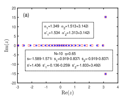
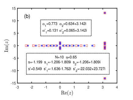
Figure 1: The distributions of zero roots with certain model parameters at the ground state. (a) The pattern includes the real roots and two additional roots at the boundary. (b) The pattern includes the real roots, two boundary strings at the origin, two boundary strings and two additional roots at the boundary. The red squares specify the roots of Bethe-ansatz-like equations (5.6)-(5.8) with the inhomogeneity parameters $\{\bar{\theta}_{k}=-i\theta_{k}=0.13k\}$ and the blue asterisks indicate the roots in the homogeneous limit obtained by the exact diagonalization of Hamiltonian. We see that the inhomogeneity parameters do not affect the imaginary parts of roots but the positions in the real axis.

The numerical solutions of the Bethe-ansatz-like equations (5.6)-(5.8) and exact numerical diagonalization results with certain model parameters at the ground state are shown in Fig.1. Fig.1(a) shows the case that there is no the boundary string. The pattern of zero roots includes the real roots and two additional roots at the boundary. The pattern of Fig.1(b) includes the real roots, four boundary strings (two of them at the origin and two at the boundary) and two additional roots at the boundary. We note that the imaginary inhomogeneity parameters almost do not affect the imaginary parts of zero roots but the positions in the real axis.

5.3 Surface energy of $XXZ$ spin-1/2 chain

We first consider the case that there is no the boundary string, where all $\text{Re}(\alpha_{x}^{y})>2\eta$. The zero roots at the ground state include the real roots $\{\bar{z}_{k}\}$ and the additional roots $\{\pi\pm z_{a}i\}$, where $z_{a}$ is real. In the thermodynamic limit, where the system size $N$ tends to infinity, the distribution of zero roots can be characterized by a density per site $\rho(\bar{z})$. Furthermore, we assume that the inhomogeneity parameters also has a continuum density per site $\sigma(\bar{\theta}_{j})\sim 1/N(\bar{\theta}_{j}-\bar{\theta}_{j-1})$, where $\bar{\theta}_{j}=-i\theta_{j}$. Thus the density of zero roots $\rho(\bar{z})$ can be derived with the help of an auxiliary function $\sigma(\bar{\theta})$ which is a given density of the inhomogeneity.

Substituting the pattern of zero roots at the ground state into the Bethe-ansatz-like equations (5.6), taking the logarithm, making the difference of the resulted equations for $\theta_{j}$ and $\theta_{j-1}$, in the thermodynamic limit, we obtain

$$N\int_{-\pi}^{\pi}b_{2}(u-\bar{z})\rho(\bar{z})d\bar{z}+b_{\frac{z_{a}}{\eta}+2}(u-\pi)+b_{\frac{z_{a}}{\eta}-2}(u-\pi)$$

$$=N\int_{-\pi}^{\pi}[b_{4}(u-\bar{\theta})+b_{4}(u+\bar{\theta})]\sigma(\bar{\theta})d\bar{\theta}+b_{4}(u-\pi)+b_{4}(u)$$

$$-b_{2}(u)-b_{2}(u-\pi)+b_{\frac{\alpha_{1}}{\eta}}(u-\pi)+b_{\frac{\alpha_{1}^{\prime}}{\eta}}(u-\pi)+b_{\frac{\bar{\alpha}_{2}}{\eta}}(u)+b_{\frac{\bar{\alpha}_{2}^{\prime}}{\eta}}(u),$$ (5.14)

where the functions $a_{n}(u)$ and $b_{n}(u)$ are defined as

$$a_{n}(u)=(\ln\sin\frac{u+n\eta i}{2}-\ln\sin\frac{u-n\eta i}{2})^{\prime}=\frac{1}{2}(\cot\frac{u+n\eta i}{2}-\cot\frac{u-n\eta i}{2}),$$

$$b_{n}(u)=(\ln\sin\frac{u+n\eta i}{2}+\ln\sin\frac{u-n\eta i}{2})^{\prime}=\frac{1}{2}(\cot\frac{u+n\eta i}{2}+\cot\frac{u-n\eta i}{2}).$$ (5.15)

Eq.(5.14) is a standard convolution integral equation and can be solved by the Fourier transformation. The Fourier transformations of Eq.(5.14) is

$$N\tilde{b}_{2}(k)\tilde{\rho}(k)+\tilde{b}_{\frac{z_{a}}{\eta}+2}(k)e^{-ik\pi}+\tilde{b}_{\frac{z_{a}}{\eta}-2}(k)e^{-ik\pi}=2N\tilde{b}_{4}(k)\tilde{\sigma}(k)+\tilde{b}_{4}(k)e^{ik\pi}+\tilde{b}_{4}(k)$$

$$-\tilde{b}_{2}(k)-\tilde{b}_{2}(k)e^{-ik\pi}+\tilde{b}_{\frac{\alpha_{1}}{\eta}}(k)e^{-ik\pi}+\tilde{b}_{\frac{\alpha_{1}^{\prime}}{\eta}}(k)e^{-ik\pi}+\tilde{b}_{\frac{\bar{\alpha}_{2}}{\eta}}(k)+\tilde{b}_{\frac{\bar{\alpha}_{2}^{\prime}}{\eta}}(k),$$ (5.16)

where $\tilde{a}_{n}(k)$ and $\tilde{b}_{n}(k)$ are calculated as

$$\tilde{a}_{n}(k)=\int_{-\pi}^{\pi}a_{n}(u)e^{-iku}du=-2\pi i\,\text{sign}(k)e^{-|n\eta k|},$$

$$\tilde{b}_{n}(k)=\int_{-\pi}^{\pi}b_{n}(u)e^{-iku}du=-2\pi i\,\text{sign}(n\eta)e^{-|n\eta k|}.$$ (5.17)

In the homogeneous limit, we take $\sigma(\bar{\theta})=\delta(\bar{\theta})$. Thus $\tilde{\sigma}(k)=1$. From Eq.(5.16), we obtain the density of zero roots as

$$\tilde{\rho}(k) = 2e^{-2\eta|k|}+\frac{1}{N}[e^{-2\eta|k|}e^{ik\pi}+e^{-2\eta|k|}-1-e^{-ik\pi}+e^{-(\alpha_{1}-2\eta)|k|}e^{-ik\pi}+e^{-(\alpha_{1}^{\prime}-2\eta)|k|}e^{-ik\pi}$$ (5.18)

$$+e^{-(\bar{\alpha}_{2}-2\eta)|k|}+e^{-(\bar{\alpha}_{2}^{\prime}-2\eta)|k|}-e^{-z_{a}|k|}e^{-ik\pi}-e^{-(z_{a}-4\eta)|k|}e^{-ik\pi}].$$

The inverse Fourier transformation gives

$$\rho(u) = \frac{i}{\pi}a_{2}(u)+\frac{i}{2\pi N}[a_{2}(u-\pi)+a_{2}(u)+a_{\frac{\alpha_{1}}{\eta}-2}(u-\pi)+a_{\frac{\alpha_{1}^{\prime}}{\eta}-2}(u-\pi)+a_{\frac{\bar{\alpha}_{2}}{\eta}-2}(u)$$ (5.19)

$$+a_{\frac{\bar{\alpha}_{2}^{\prime}}{\eta}-2}(u)-a_{\frac{z_{a}}{\eta}}(u-\pi)-a_{\frac{z_{a}}{\eta}-4}(u-\pi)]-\frac{1}{N}[\delta(u)+\delta(u-\pi)].$$

Thus the ground state energy of the Hamiltonian (5.1) is

$$E^{s+}_{g} = -\frac{N}{4}\int_{-\pi}^{\pi}\coth\frac{2\eta+zi}{2}\rho(z)dz+\frac{\tanh(2\eta)}{4}(1+\coth s^{\prime})$$ (5.20)

$$-\frac{1}{4}[\tanh\frac{2\eta+z_{a}}{2}+\tanh\frac{2\eta-z_{a}}{2}]$$

$$= -\frac{N}{2}\coth(2\eta)-\frac{1}{4}[\coth(2\eta)-\coth\eta-\tanh\eta+\tanh\frac{\alpha_{1}}{2}+\tanh\frac{\alpha^{\prime}_{1}}{2}$$

$$+\coth\frac{\bar{\alpha}_{2}}{2}+\coth\frac{\bar{\alpha}^{\prime}_{2}}{2}-\tanh(2\eta)\coth s^{\prime}+2\tanh\frac{2\eta-z_{a}}{2}].$$

Now, we prove that the $z_{a}$ tends to infinity in the thermodynamic limit. Taking the logarithm of Eq.(5.7) and considering the homogeneous limit $\{\theta_{j}=0\}$, we have

$$\log\Lambda_{0}+N\log(-1)+\sum^{2N+4}_{k=1}\log\sin\frac{z_{k}-2\eta i}{2}=\log 2+\log\cosh(2\eta)$$

$$+\log\sinh s+\log\sinh s^{\prime}+2N\log\sinh(2\eta).$$ (5.21)

In the thermodynamic limit, Eq.(5.21) reads

$$\log\Lambda_{0}+N\log(-1)+N\int^{\pi}_{-\pi}\log\sin\frac{\bar{z}-2\eta i}{2}\rho(\bar{z})d\bar{z}+\log\cosh\frac{2\eta-z_{a}}{2}+\log\cosh\frac{2\eta+z_{a}}{2}$$

$$=\log 2+\log\cosh(2\eta)+\log\sinh s+\log\sinh s^{\prime}+2N\log\sinh(2\eta).$$ (5.22)

Substituting the density (5.19) into (5.22) and omitting the $O(N^{-1})$ terms, we have

$$z_{a} = 2N\log\sinh(2\eta)-\frac{iN}{\pi}\int_{-\pi}^{\pi}\log\sin\frac{\bar{z}-2\eta i}{2}a_{2}(\bar{z})d\bar{z}+C$$ (5.23)

$$= 2\eta N+C^{\prime},$$

where $C^{\prime}$ is a constant irrelevant with $N$. Thus $z_{a}$ tends to infinity if $N\rightarrow\infty$. The same result can also be obtained by using the Bethe-ansatz-like equations (5.8) with the similar method.

Next, we check the conclusion (5.23) numerically. By using the exact numerical diagonalization method, we obtain the values of $z_{a}$ with certain model parameters. In the homogeneous limit, the values of $z_{a}$ for different system sizes are shown in Fig.2. The data can be fitted as $aN+b$. From the fitting, we see that $a=2\eta$ and $b=1.758$ which is irrelevant with $N$.

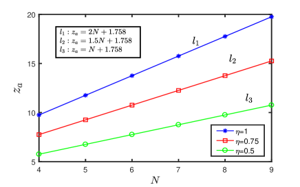
Figure 2: The finite size scaling behaviors of $z_{a}$. The blue asterisks, red squares and green circles are the numerical solutions of $z_{a}$ with $\eta=0.5$, $0.75$ and $1$, respectively. The data can be fitted as $aN+b$. It is clear that $a=2\eta$, $b=1.758$, and $z_{a}\rightarrow\infty$ if $N\rightarrow\infty$. Here the model parameters are $h_{1}^{+}=0.23+0.36i$, $h_{1}^{-}=0.23-0.36i$, $h_{1}^{z}=1.2$, $h_{N}^{+}=0.82+0.93i$, $h_{N}^{-}=0.82-0.93i$ and $h_{N}^{z}=3.23$.

Now, we are ready to calculate the surface energy of the Hamiltonian (5.1). The surface energy is defined by

$$E^{s+}_{s}=E^{s+}_{g}-E^{sp}_{g},$$ (5.24)

where $E^{s+}_{g}$ is the ground state energy given by (5.20) and

$$E^{sp}_{g}=-\frac{N}{2}\coth 2\eta,$$ (5.25)

is the ground state energy of the system with periodic boundary condition

$$H^{sp}=-\sum_{j=1}^{N}\frac{1}{4\sinh 2\eta}[\sigma^{x}_{j}\sigma^{x}_{j+1}+\sigma^{y}_{j}\sigma^{y}_{j+1}+\cosh(2\eta)\sigma^{z}_{j}\sigma^{z}_{j+1}]-\frac{N}{4}\coth 2\eta.$$ (5.26)

Considering $z_{a}\rightarrow\infty$ in the thermodynamic limit, we obtain the surface energy as

$$E^{s+}_{s} = \frac{1}{2}-\frac{1}{4}[\coth(2\eta)-\coth\eta-\tanh\eta+\tanh\frac{\alpha_{1}}{2}+\tanh\frac{\alpha^{\prime}_{1}}{2}$$ (5.27)

$$+\coth\frac{\bar{\alpha}_{2}}{2}+\coth\frac{\bar{\alpha}^{\prime}_{2}}{2}-\tanh(2\eta)\coth s^{\prime}].$$

Next, we consider the case that there exists one boundary string. For example, we choose the boundary parameters in the regime of $\alpha_{1}<2\eta$, $\alpha_{1}^{\prime}>2\eta$, $\text{Re}(\alpha_{2})>2\eta$ and $\text{Re}(\alpha_{2}^{\prime})>2\eta$. In this case, only the boundary string $\pi\pm(2\eta-\alpha_{1})i$ exists. This boundary string would affect the distribution of zero roots and make the density $\rho(z)$ has a deviation. After some calculations, we obtain the deviation $\delta\tilde{\rho}(k)$ as

$$\delta\tilde{\rho}(k)=-\frac{1}{N}[e^{-(2\eta-\alpha_{1})|k|}+e^{(2\eta-\alpha_{1})|k|}]e^{-ik\pi}.$$ (5.28)

The contribution of boundary string to the ground state energy is

$$\delta E^{s+}_{g}=-\frac{N}{4}\int_{-\pi}^{\pi}\coth\frac{2\eta+zi}{2}\delta\rho(z)dz-\frac{1}{4}(\tanh\frac{\alpha_{1}}{2}+\tanh\frac{4\eta-\alpha_{1}}{2})=0.$$ (5.29)

Thus the boundary string contributes nothing to the ground state energy. The ground state energy (5.20) and surface energy (5.27) are correct for the all regimes of boundary parameters.

The ground state energy of the Hamiltonian $H^{s-}$ can be obtained similarly

$$E^{s-}_{g}=E^{s+}_{g}|_{\{\alpha_{1},\alpha^{\prime}_{1},\alpha_{2},\alpha^{\prime}_{2}\}\rightarrow\{\gamma_{1},\gamma^{\prime}_{1},\gamma_{2},\gamma^{\prime}_{2}\}},$$ (5.30)

where the boundary parameters are defined as

$$\gamma=\frac{1}{2t_{1}t_{2}},\quad\cosh\gamma_{1}=\frac{\gamma}{2}+\xi,\quad\cosh\gamma_{2}=\frac{\gamma}{2}-\xi,\quad\xi=\sqrt{1+\frac{\gamma^{2}}{4}+\gamma\cosh(2t)},$$

$$\gamma^{\prime}=\frac{1}{2t^{\prime}_{1}t^{\prime}_{2}},\,\,\cosh\gamma^{\prime}_{1}=\frac{\gamma^{\prime}}{2}+\xi^{\prime},\,\,\cosh\gamma^{\prime}_{2}=\frac{\gamma^{\prime}}{2}-\xi^{\prime},\quad\xi^{\prime}=\sqrt{1+\frac{\gamma^{\prime 2}}{4}+\gamma^{\prime}\cosh(2t^{\prime})}.$$ (5.31)

The selection rules of $\gamma_{x}^{y}\in\{\gamma_{1},\gamma^{\prime}_{1},\gamma_{2},\gamma^{\prime}_{2}\}$ are that all the $\text{Re}(\gamma^{y}_{x})$ take positive values if $\coth s\coth s^{\prime}<0$; or the smaller $\text{Re}(\gamma^{y}_{x})$ in the set $\gamma^{y}_{x}\in\{\gamma_{1},\gamma^{\prime}_{1}\}$ takes the negative value and the others remain positive if $\coth s\coth s^{\prime}>0$. Similar to $\alpha_{2}$ and $\alpha_{2}^{\prime}$, we denote $\gamma_{2}=\bar{\gamma}_{2}+\pi i$ and $\gamma^{\prime}_{2}=\bar{\gamma}^{\prime}_{2}+\pi i$, where $\bar{\gamma}_{2}$ and $\bar{\gamma}^{\prime}_{2}$ are real.

5.4 Surface energy of the anisotropic $D^{(1)}_{2}$ spin chain

Now, we are ready to calculate the surface energy of the anisotropic $D^{(1)}_{2}$ spin chain. The ground state energy of the system (4.15) with the twisted boundary magnetic fields is

$$E_{g} = -N\coth(2\eta)+1-\frac{1}{4}[2\coth(2\eta)-2\coth\eta-2\tanh\eta+\tanh\frac{\alpha_{1}}{2}+\tanh\frac{\alpha^{\prime}_{1}}{2}$$ (5.32)

$$+\coth\frac{\bar{\alpha}_{2}}{2}+\coth\frac{\bar{\alpha}^{\prime}_{2}}{2}-\tanh(2\eta)\coth s^{\prime}+\tanh\frac{\gamma_{1}}{2}+\tanh\frac{\gamma^{\prime}_{1}}{2}$$

$$+\coth\frac{\bar{\gamma}_{2}}{2}+\coth\frac{\bar{\gamma}^{\prime}_{2}}{2}-\tanh(2\eta)\coth t^{\prime}].$$

The Hamiltonian of anisotropic $D^{(1)}_{2}$ spin chain with periodic boundary condition is

$$H^{p}=-\sum_{j=1}^{N}\frac{1}{4\sinh(2\eta)}\{\cosh(2\eta)(\sigma^{z}_{j}\sigma^{z}_{j+1}+\tau^{z}_{j}\tau^{z}_{j+1})+2[\sigma^{z}_{j}\sigma^{z}_{j+1}(\tau^{+}_{j}\tau^{-}_{j+1}+\tau^{-}_{j}\tau^{+}_{j+1})$$

$$\qquad+(\sigma^{+}_{j}\sigma^{-}_{j+1}+\sigma^{-}_{j}\sigma^{+}_{j+1})\tau^{z}_{j}\tau^{z}_{j+1}]\}-\frac{N}{2}\coth(2\eta).$$ (5.33)

The ground state energy of the Hamiltonian (5.33) is

$$E^{p}_{g}=-N\coth(2\eta).$$ (5.34)

Thus the surface energy of anisotropic $D^{(1)}_{2}$ spin chain reads

$$E_{s} = 1-\frac{1}{4}[2\coth(2\eta)-2\coth\eta-2\tanh\eta+\tanh\frac{\alpha_{1}}{2}+\tanh\frac{\alpha^{\prime}_{1}}{2}$$ (5.35)

$$+\coth\frac{\bar{\alpha}_{2}}{2}+\coth\frac{\bar{\alpha}^{\prime}_{2}}{2}-\tanh(2\eta)\coth s^{\prime}+\tanh\frac{\gamma_{1}}{2}+\tanh\frac{\gamma^{\prime}_{1}}{2}$$

$$+\coth\frac{\bar{\gamma}_{2}}{2}+\coth\frac{\bar{\gamma}^{\prime}_{2}}{2}-\tanh(2\eta)\coth t^{\prime}],$$

where the parameters $\alpha,\alpha_{1},etc.$ are given by (4.5) and (5.31). The energy expression (5.35) is valid for $\eta>0$ and all the other fundamental parameters ($s,s_{1},s_{2},etc.$) which keep the Hamiltonian (4.15) hermitian (eg. $s=s^{*}$, $s_{1}=s_{2}^{*}$, $s^{\prime}=s^{\prime*}$, $s_{1}^{\prime}=e^{(s_{r}+is_{i})\eta}$, $s_{2}^{\prime}=e^{(s_{r}+4-is_{i})\eta}$, $t=t^{*}$, $t_{1}=t_{2}^{*}$, $t^{\prime}=t^{\prime*}$, $t_{1}^{\prime}=e^{(t_{r}+it_{i})\eta}$, $t_{2}^{\prime}=e^{(t_{r}+4-it_{i})\eta}$, where $s_{r},s_{i},t_{r},t_{i}$ are real, and the superscript * means the complex conjugate).

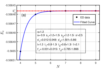
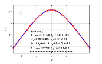
Figure 3: (a) The finite size scaling behavior of the surface energy $E_{s}$ of the anisotropic $D^{(1)}_{2}$ spin chain. The black points are calculated from the exact diagonalization method with the finite system size $N$. The data can be fitted as $E_{s}=-0.778485e^{-2.44378N}-0.566456$. When $N$ tends to infinity, the finite size scaling analysis gives the value $-0.566456$, which is exactly the same as the surface energy calculated from the analytic expression (5.35). (b) The surface energy $E_{s}$ versus the boundary parameter $x=\text{Re}(s_{1})$. The blue line indicates the analytic result and the red squares indicate the numerical results. They are consistent with each other very well.

We check the conclusion (5.35) numerically. The surface energy can also be calculated by using the exact diagonalization method with the help of finite size scaling analysis. Here, the exact diagonalization is performed with the anisotropic $\eta=1.2$ and the system size $N$ is set from 4 to 9. The results are shown in Fig.3. The exact diagonalization results with the fixed boundary parameters are shown in Fig.3(a). The date can be fitted as $E_{s}=-0.778485e^{-2.44378N}-0.566456$. When $N$ tends to infinity, the finite size scaling analysis gives the value $-0.566456$, which is exactly the same as the surface energy calculated from the analytic expression (5.35). In Fig.3(b), we show the surface energy versus one free boundary parameter. Again, the analytic results obtained from (5.35) and the numerical ones calculated from exact diagonalization are consistent with each other very well.

6 Results for the isotropic $D^{(1)}_{2}$ spin chain

6.1 Exact solution

The isotropic $D^{(1)}_{2}$ spin chain is quantified by the transfer matrix

$$\tilde{t}(u)=tr_{0}\{\bar{\tilde{K}}_{0}(u)\tilde{R}_{01}(u-\theta_{1})\cdots\tilde{R}_{0N}(u-\theta_{N})\tilde{K}_{0}(u)\tilde{R}_{N0}(u+\theta_{N})\cdots\tilde{R}_{10}(u+\theta_{1})\}.$$ (6.1)

Here the dual reflection matrix $\bar{\tilde{K}}(u)$ can be obtained from the reflection matrix $\tilde{K}(u)$ by the mapping

$$\bar{\tilde{K}}(u)=\tilde{K}(-u-1)|_{\{t,t_{1},t_{2},s,s_{1},s_{2}\}\rightarrow\{t^{\prime},t^{\prime}_{1},t^{\prime}_{2},s^{\prime},s^{\prime}_{1},s^{\prime}_{2}\}},$$ (6.2)

and $\tilde{K}(u)$ is the $4\times 4$ matrix with the elements

$$\tilde{k}_{11}(u)=(s-u)(t-u),\quad\tilde{k}_{12}(u)=-t_{1}u(s-u),\quad\tilde{k}_{13}(u)=s_{1}u(t-u),$$

$$\tilde{k}_{14}(u)=s_{1}t_{1}u^{2},\quad\tilde{k}_{21}(u)=-t_{2}u(s-u),\quad\tilde{k}_{22}(u)=(s-u)(t+u),$$

$$\tilde{k}_{23}(u)=-s_{1}t_{2}u^{2},\quad\tilde{k}_{24}(u)=-s_{1}u(t+u),\quad\tilde{k}_{31}(u)=s_{2}u(t-u),$$

$$\tilde{k}_{32}(u)=-s_{2}t_{1}u^{2},\quad\tilde{k}_{33}(u)=(s+u)(t-u),\quad\tilde{k}_{34}(u)=t_{1}u(s+u),$$

$$\tilde{k}_{41}(u)=s_{2}t_{2}u^{2},\quad\tilde{k}_{42}(u)=-s_{2}u(t-u),\quad\tilde{k}_{43}(u)=t_{2}u(s+u),$$

$$\tilde{k}_{44}(u)=(s+u)(t+u).$$ (6.3)

The associated $R$-matrix reads

$$\tilde{R}_{12}(u)=\left(\begin{array}[]{cccc|cccc|cccc|cccc}\tilde{a}&&&&&&&&&&&&&&&\\ &\tilde{b}&&&\tilde{g}&&&&&&&&&&&\\ &&\tilde{b}&&&&&&\tilde{g}&&&&&&&\\ &&&\tilde{e}&&&\tilde{d}&&&\tilde{d}&&&\tilde{c}&&&\\ \hline\cr&\tilde{g}&&&\tilde{b}&&&&&&&&&&&\\ &&&&&\tilde{a}&&&&&&&&&&\\ &&&\tilde{d}&&&\tilde{e}&&&\tilde{c}&&&\tilde{d}&&&\\ &&&&&&&\tilde{b}&&&&&&\tilde{g}&&\\ \hline\cr&&\tilde{g}&&&&&&\tilde{b}&&&&&&&\\ &&&\tilde{d}&&&\tilde{c}&&&\tilde{e}&&&\tilde{d}&&&\\ &&&&&&&&&&\tilde{a}&&&&&\\ &&&&&&&&&&&\tilde{b}&&&g&\\ \hline\cr&&&\tilde{c}&&&\tilde{d}&&&\tilde{d}&&&\tilde{e}&&&\\ &&&&&&&\tilde{g}&&&&&&\tilde{b}&&\\ &&&&&&&&&&&\tilde{g}&&&\tilde{b}&\\ &&&&&&&&&&&&&&&\tilde{a}\\ \end{array}\right),$$ (6.20)

where the matrix elements are

$$\tilde{a}=(u+1)(u+1),\;\;\tilde{b}=u(u+1),\;\;\tilde{c}=1,\;\;\tilde{d}=-u,\;\;\tilde{e}=u^{2},\;\;\tilde{g}=u+1.$$

The reflection matrices (6.2)-(6.3) can be factorized as

$$\bar{\tilde{K}}(u)=S[\bar{\tilde{K}}^{s+}(u)\otimes\bar{\tilde{K}}^{s-}(u)]S^{-1},\quad\tilde{K}(u)=S[\tilde{K}^{s+}(u)\otimes\tilde{K}^{s-}(u)]S^{-1},$$ (6.21)

where the matrix $S$ is given by Eq.(3.2) and

$$\bar{\tilde{K}}^{s+}(u)=\tilde{K}^{s+}(-u-1)|_{\{s,s_{1},s_{2}\}\rightarrow\{s^{\prime},s^{\prime}_{1},s^{\prime}_{2}\}},\quad\tilde{K}^{s+}(u)=\left(\begin{array}[]{cc}s-u&s_{1}u\\ s_{2}u&s+u\end{array}\right),$$ (6.24)

$$\bar{\tilde{K}}^{s-}(u)=\tilde{K}^{s+}(-u-1)|_{\{t,t_{1},t_{2}\}\rightarrow\{t^{\prime},t^{\prime}_{1},t^{\prime}_{2}\}},\quad\tilde{K}^{s-}(u)=\tilde{K}^{s-}(u)|_{\{s,s_{1},s_{2}\}\rightarrow\{t,t_{1},t_{2}\}}.$$ (6.25)

The $R$-matrix (6.20) can be decomposed into

$$\tilde{R}_{12}(u)=[S\otimes S][\tilde{R}^{s}_{1^{\prime}2^{\prime}}(u)\otimes\tilde{R}^{s}_{1^{\prime\prime}2^{\prime\prime}}(u)][S\otimes S]^{-1},$$ (6.26)

where $\tilde{R}^{s}_{1^{\prime}2^{\prime}}(u)$ is the $R$-matrix of the isotropic XXX spin chain

$$\tilde{R}^{s}_{1^{\prime}2^{\prime}}(u)=\left(\begin{array}[]{cccc}u+1&0&0&0\\ 0&u&1&0\\ 0&1&u&0\\ 0&0&0&u+1\end{array}\right).$$ (6.31)

Based on the above decompositions, we obtain the eigenvalue of transfer matrix (6.1) as

$$\tilde{\Lambda}(u)=\tilde{\Lambda}^{s+}(u)\tilde{\Lambda}^{s-}(u),$$ (6.32)

where

$$\tilde{\Lambda}^{s+}(u)=\frac{u+1}{u-\frac{1}{2}}(s+\sqrt{1+s_{1}s_{2}}u)(s^{\prime}-\sqrt{1+s^{\prime}_{1}s^{\prime}_{2}}u)\tilde{a}(u)\frac{\tilde{Q}(u-1)}{\tilde{Q}(u)}$$

$$\quad\quad\quad+\frac{u}{u-\frac{1}{2}}[s-\sqrt{1+s_{1}s_{2}}(u+1)][s^{\prime}+\sqrt{1+s^{\prime}_{1}s^{\prime}_{2}}(u+1)]\tilde{d}(u)\frac{\tilde{Q}(u+1)}{\tilde{Q}(u)}$$

$$\quad\quad\quad+\tilde{x}_{+}u(u+1)\frac{\tilde{a}(u)\tilde{d}(u)}{\tilde{Q}(u)},$$

$$\tilde{\Lambda}^{s-}(u)=\tilde{\Lambda}^{s+}(u)|_{\{s,s_{1},s_{2},s^{\prime},s^{\prime}_{1},s^{\prime}_{2}\}\rightarrow\{t,t_{1},t_{2},t^{\prime},t^{\prime}_{1},t^{\prime}_{2}\}},$$ (6.33)

and

$$\tilde{Q}(u)=\prod_{l=1}^{N}(u-\mu_{l})(u+\mu_{l}+1),$$

$$\tilde{a}(u)=\prod_{j=1}^{N}(u-\theta_{j}+1)(u+\theta_{j}+1)=\tilde{d}(u+1),$$

$$\tilde{x}_{+}=2\sqrt{(1+s_{1}s_{2})(1+s^{\prime}_{1}s^{\prime}_{2})}-(2+s_{1}s^{\prime}_{2}+s_{2}s^{\prime}_{1}).$$ (6.34)

The Bethe roots $\{u_{l}\}$ in Eq.(6.33) should satisfy the Bethe ansatz equations

$$\frac{\mu_{l}+1}{\mu_{l}-\frac{1}{2}}\frac{(s+\sqrt{1+s_{1}s_{2}}\mu_{l})(s^{\prime}-\sqrt{1+s^{\prime}_{1}s^{\prime}_{2}}\mu_{l})}{\tilde{d}(u_{l})}{\tilde{Q}(\mu_{l}-1)}$$

$$+\frac{\mu_{l}}{\mu_{l}-\frac{1}{2}}\frac{[s-\sqrt{1+s_{1}s_{2}}(\mu_{l}+1)[[s^{\prime}+\sqrt{1+s^{\prime}_{1}s^{\prime}_{2}}(\mu_{l}+1)]}{\tilde{a}(u_{l})}{\tilde{Q}(\mu_{l}+1)}$$

$$=-\tilde{x}_{+}\mu_{l}(\mu_{l}+1),\quad l=1,\cdots,N.$$ (6.35)

The Hamiltonian of isotropic $D^{(1)}_{2}$ spin chain generated by the transfer matrix (6.1) is

$$\tilde{H}=\sum_{j=1}^{N-1}[\frac{1}{2}(\sigma^{z}_{j}\sigma^{z}_{j+1}+\tau^{z}_{j}\tau^{z}_{j+1})+\sigma^{z}_{j}\sigma^{z}_{j+1}(\tau^{+}_{j}\tau^{-}_{j+1}+\tau^{-}_{j}\tau^{+}_{j+1})+(\sigma^{+}_{j}\sigma^{-}_{j+1}+\sigma^{-}_{j}\sigma^{+}_{j+1})\tau^{z}_{j}\tau^{z}_{j+1}]$$

$$\qquad-\frac{1}{2st}(s\tau^{z}_{N}+t\sigma^{z}_{N}+st_{1}\sigma^{z}_{N}\tau^{+}_{N}-s_{1}t\sigma^{+}_{N}\tau^{z}_{N}+st_{2}\sigma^{z}_{N}\tau^{-}_{N}-s_{2}t\sigma^{-}_{N}\tau^{z}_{N})$$

$$\qquad+\frac{1}{2s^{\prime}t^{\prime}}(s^{\prime}\tau^{z}_{1}+t^{\prime}\sigma^{z}_{1}+s^{\prime}t^{\prime}_{1}\sigma^{z}_{1}\tau^{+}_{1}-s^{\prime}_{1}t^{\prime}\sigma^{+}_{1}\tau^{z}_{1}+s^{\prime}t^{\prime}_{2}\sigma^{z}_{1}\tau^{-}_{1}+s^{\prime}_{2}t^{\prime}\sigma^{-}_{1}\tau^{z}_{1})+N.$$ (6.36)

We find that the Hamiltonian (6.36) is the direct summation of two XXX spin-1/2 chains with non-diagonal boundary magnetic fields up to the similar transformation ${\cal S}$

$$\tilde{H}={\cal S}[\tilde{H}^{s+}\oplus\tilde{H}^{s-}]{\cal S}^{-1},$$ (6.37)

where

$$\tilde{H}^{s+}=\sum_{j=1}^{N-1}\frac{1}{2}(\sigma^{x}_{j}\sigma^{x}_{j+1}+\sigma^{y}_{j}\sigma^{y}_{j+1}+\sigma^{z}_{j}\sigma^{z}_{j+1})+\frac{1}{4s}(s_{1}+s_{2})\sigma^{x}_{N}+\frac{i}{4s}(s_{1}-s_{2})\sigma^{y}_{N}-\frac{1}{2s}\sigma^{z}_{N}$$

$$\quad\qquad-\frac{1}{4s^{\prime}}(s^{\prime}_{1}+s^{\prime}_{2})\sigma^{x}_{1}-\frac{i}{4s^{\prime}}(s^{\prime}_{1}-s^{\prime}_{2})\sigma^{y}_{1}+\frac{1}{2s^{\prime}}\sigma^{z}_{1}+\frac{N}{2},$$ (6.38)

$$\tilde{H}^{s-}=\tilde{H}^{s+}|_{\{\sigma_{j}^{\alpha},s,s_{1},s_{2},s^{\prime},s^{\prime}_{1},s^{\prime}_{2}\}\rightarrow\{\tau_{j}^{\alpha},t,t_{1},t_{2},t^{\prime},t^{\prime}_{1},t^{\prime}_{2}\}},$$ (6.39)

with ${\cal{S}}=\otimes^{N}S$ and $S=\frac{1}{2}(1-\sigma^{z}+\tau^{z}+\sigma^{z}\tau^{z})$. The conclusion (6.37) is consistent with the fact that the corresponding $R$-matrix and reflection matrices in the transfer matrix $\tilde{t}(u)$ of the system can be factorized. The eigenvalue of the Hamiltonian (6.36) is

$$\tilde{E}^{s+}=\frac{\partial\ln\tilde{\Lambda}(u)}{2\partial u}|_{u=0,\{\theta_{j}\}=0},$$ (6.40)

where $\tilde{\Lambda}(u)$ is given by Eq.(6.32). In the derivation, the identity $tr_{0}{\bar{\tilde{K}}_{0}}(0)^{\prime}=0$ is used.

6.2 Symmetry

In the Hamiltonian (6.38), there are six free boundary parameters. However, due to the fact that the interactions in the bulk are isotropic and have the $su(2)$ symmetry, the free boundary parameters can be reduced. The method is as follows. First, we choose the direction of magnetic field at the left side as the $z$-direction, which can be achieved by acting the transformation matrix $\otimes_{j=1}^{N}\tilde{C}_{j}^{1}$ on the Hamiltonian (6.38). Then, we take a rotation of the resulted Hamiltonian in the $xy$ plane to make the direction of magnetic field at the right side lying in the $xz$ plane. This can be achieved by using the transition matrix $\otimes_{j=1}^{N}\tilde{C}^{2}_{j}$. We note that the interactions in the bulk do not change after the transformations.

The final result is

$$\bar{H}^{s+} = \otimes_{j=1}^{N}[\tilde{C}^{2}_{j}]^{-1}[\tilde{C}^{1}_{j}]^{-1}\tilde{H}^{s+}\tilde{C}^{1}_{j}\tilde{C}^{2}_{j}$$ (6.41)

$$= \frac{1}{2}\bigg{[}\sum_{j=1}^{N-1}(\sigma^{x}_{j}\sigma^{x}_{j+1}+\sigma^{y}_{j}\sigma^{y}_{j+1}+\sigma^{z}_{j}\sigma^{z}_{j+1})+\frac{1}{p}\sigma^{z}_{1}+\frac{1}{q}(\xi\sigma^{x}_{N}+\sigma^{z}_{N})\bigg{]}+\frac{N}{2}.$$

Here the transformation matrices $\tilde{C}^{1}_{j}$ and $\tilde{C}^{2}_{j}$ are

$$\tilde{C}^{1}_{j}=\left(\begin{array}[]{cc}C^{1}_{11}&C^{1}_{12}\\ C^{1}_{21}&C^{1}_{22}\end{array}\right)_{[j]},\quad\tilde{C}^{2}_{j}=\left(\begin{array}[]{cc}C^{2}_{11}&0\\ 0&1\end{array}\right)_{[j]},$$ (6.46)

and the matrix elements are

$$C^{1}_{11} \!\!\!= \!\!\!\frac{s_{1}^{\prime}\left(\bar{s}_{1}-1\right)}{\left|s_{1}^{\prime}\right|\sqrt{2\bar{s}_{1}(\bar{s}_{1}-1)}},\qquad C^{1}_{12}=-\frac{s_{1}^{\prime}\sqrt{\bar{s}_{1}+1}}{\sqrt{2\bar{s}_{1}}\left|s_{1}^{\prime}\right|},\qquad\bar{s}_{1}=\sqrt{\left|s_{1}^{\prime}\right|^{2}+1},$$

$$C^{1}_{21} \!\!\!= \!\!\!\frac{\left|s_{1}^{\prime}\right|}{\sqrt{2\bar{s}_{1}(\bar{s}_{1}-1)}},\qquad C^{1}_{22}=\frac{\left|s_{1}^{\prime}\right|}{\sqrt{2(\left|s_{1}^{\prime}\right|^{2}+\bar{s}_{1}+1)}},$$

$$C^{2}_{11} \!\!\!= \!\!\!s_{1}^{\prime}s_{1}\sqrt{\bar{s}_{1}-\bar{s}_{1}^{2}}\left[s_{1}\left(s_{1}^{\prime*}\right)^{2}+2\left(\bar{s}_{1}+1\right)s_{1}^{\prime*}-s_{1}^{*}\left(\bar{s}_{1}+1\right)^{2}\right]\left[s_{1}^{\prime*}\left(\bar{s}_{1}^{2}+\bar{s}_{1}\right)\right]^{-1}$$ (6.47)

$$\!\!\!\times \!\!\!\left\{s_{1}^{\prime 2}s_{1}^{2}\left[s_{1}^{*}\left(s_{1}^{\prime 2}s_{1}^{*}+4s_{1}^{\prime}-4s_{1}\right)+s_{1}^{2}\left(s_{1}^{\prime*}\right)^{2}-2s_{1}^{\prime*}\left(s_{1}^{\prime}s_{1}s_{1}^{*}+2s_{1}^{\prime}-2s_{1}\right)\right]\right\}^{-\frac{1}{2}}.$$

The boundary parameters $p$, $q$ and $\xi$ in the Hamiltonian (6.41) reads

$$p \!\!\!= \!\!\!-s^{\prime}(\left|s_{1}^{\prime}\right|^{2}+1)^{-\frac{1}{2}},\qquad q=2s(\left|s_{1}^{\prime}\right|^{2}+1)^{\frac{1}{2}}(s_{1}s_{1}^{\prime*}+s_{1}^{\prime}s_{1}^{*}+2)^{-1},$$

$$\xi \!\!\!= \!\!\!\left\{-s_{1}^{\prime 2}s_{1}^{2}\left[s_{1}^{*}\left(s_{1}^{\prime 2}s_{1}^{*}+4s_{1}^{\prime}-4s_{1}\right)+s_{1}^{2}\left(s_{1}^{\prime*}\right)^{2}-2s_{1}^{\prime*}\left(s_{1}^{\prime}s_{1}s_{1}^{*}+2s_{1}^{\prime}-2s_{1}\right)\right]\right\}^{\frac{1}{2}}$$ (6.48)

$$\times\left[s_{1}^{\prime}s_{1}\left(s_{1}s_{1}^{\prime*}+s_{1}^{\prime}s_{1}^{*}+2\right)\right]^{-1}.$$

We see that only three free boundary parameters are left. The hermitian of Hamiltonian (6.41) requires that all the $p$, $q$ and $\xi$ are real. The Hamiltonians $\bar{H}^{s+}$ and $\tilde{H}^{s+}$ have the same eigen-energies. Thus in the following, we derive the eigenvalues of the Hamiltonians $\bar{H}^{s+}$ instead of $\tilde{H}^{s+}$.

6.3 Surface energy for the isotropic $D^{(1)}_{2}$ Hamiltonian

The Hamiltonian (6.41) is generated by the transfer matrix $\bar{t}(u)$ as

$$\bar{H}^{s+}=\left.\frac{\partial\ln\bar{t}(u)}{2\partial u}\right|_{u=0,\{\theta_{j}=0\}},$$ (6.49)

where $\bar{t}(u)$ is defined by

$$\bar{t}(u)=tr_{0}\{K^{+}_{0}(u)\tilde{R}^{s}_{0,N}(u-\theta_{N})\cdots\tilde{R}^{s}_{0,1}(u-\theta_{1})K^{-}_{0}(u)\tilde{R}^{s}_{0,1}(u+\theta_{1})\cdots\tilde{R}^{s}_{0,N}(u+\theta_{N})\},$$ (6.50)

and the reflection matrices are

$$K^{-}(u) = \left(\begin{array}[]{ll}p+u&0\\ 0&p-u\end{array}\right),$$ (6.53)

$$K^{+}(u) = \left(\begin{array}[]{ll}q+u+1&\xi(u+1)\\ \xi(u+1)&q-u-1\end{array}\right).$$ (6.56)

From the definition (6.50), we know that $\bar{t}(u)$ and its eigenvalue $\bar{\Lambda}(u)$ are the polynomials of $u$ with the degree $2N+2$. Thus we parameterize the eigenvalue $\bar{\Lambda}(u)$ by its roots $\{z_{j}\}$ as

$$\bar{\Lambda}(u)=2\prod_{j=1}^{2N+2}\left(u-z_{j}i+\frac{1}{2}\right).$$ (6.57)

Acting Eq.(6.49) on a common eigenstate of $\bar{H}^{s+}$ and $\bar{t}(u)$, we obtain the eigenvalue $\bar{E}^{s+}$ of the Hamiltonian $\bar{H}^{s+}$

$$\bar{E}^{s+}=\sum_{j=1}^{2N+2}\frac{1}{1-2\hat{z}_{j}i},$$ (6.58)

where $\{\hat{z}_{j}\}$ are the homogeneous limit of zero roots $\{z_{j}\}$. We note that Eq.(6.58) is also the energy of the Hamiltonian $\tilde{H}^{s+}$ (6.38).

The next task is to determine the values of roots $\{z_{j}\}$ that is to seek $2N+2$ constraints of roots $\{z_{j}\}$. By using the fusion technique, we obtain that the $\bar{\Lambda}(u)$ at the inhomogeneity points satisfies following functional relations

$$\bar{\Lambda}(\pm\theta_{j})\bar{\Lambda}(\pm\theta_{j}-1)=\bar{d}^{s}(\pm\theta_{j}-1)\bar{a}^{s}(\pm\theta_{j}),\quad j=1,\cdots N,$$ (6.59)

where $\bar{d}^{s}(u)=\bar{a}^{s}(-u-1)$ and $\bar{a}^{s}(u)$ is given by

$$\bar{a}^{s}(u)=\frac{u+1}{u+\frac{1}{2}}(u+p)(\sqrt{1+\xi^{2}}u+q)\prod_{j=1}^{N}(u-\theta_{j}+1)(u+\theta_{j}+1).$$ (6.60)

From the direction calculation, we also know the values of $\bar{\Lambda}(u)$ at some special points,

$$\bar{\Lambda}(0)=\bar{\Lambda}(-1)=\bar{a}^{s}(0).$$ (6.61)

Thus the $2N+2$ constrains of $\{z_{j}\}$ are

$$4\prod_{l=1}^{2N+2}(\pm\theta_{j}-z_{l}i+\frac{1}{2})(\pm\theta_{j}-z_{l}i-\frac{1}{2})=\bar{a}^{s}(\pm\theta_{j})\bar{d}^{s}(\pm\theta_{j}-1),\,j=1,\ldots,N,$$ (6.62)

$$2\prod_{j=1}^{2N+2}\left(z_{j}i\pm\frac{1}{2}\right)=\bar{a}^{s}(0),$$ (6.63)

which are the Bethe-ansatz-like equations satisfied by the zero roots $\{z_{j}\}$.

Similar with the anisotropic case, we consider that the inhomogeneity parameter are pure imaginary or zero. We denote $\theta_{k}=i\bar{\theta}_{k}$, where $\bar{\theta}_{k}$ is real. From the properties of $R$-matrix (6.31), it is easy to prove that $\bar{\Lambda}(u)$ has the crossing symmetry

$$\bar{\Lambda}(u)=\bar{\Lambda}(-u-1).$$ (6.64)

Substituting (6.57) into (6.64), we have

$$\prod_{j=1}^{2N+2}\left(u-z_{j}i+\frac{1}{2}\right)=\prod_{j=1}^{2N+2}\left(u+z_{j}i+\frac{1}{2}\right).$$ (6.65)

Thus we conclude if $z_{j}$ is a zero root of $\bar{\Lambda}(u)$, then $-z_{j}$ must be the root. One can also easily prove that

$$[\bar{t}(u)]^{\dagger}=\bar{t}(u^{*}),\quad[\bar{\Lambda}(u)]^{*}=\bar{\Lambda}(u^{*}).$$ (6.66)

Substituting (6.57) into (6.66), we have

$$\prod^{2N+2}_{k=1}\left(u^{*}+z_{k}^{*}i-\frac{1}{2}\right)=\prod^{2N+2}_{k=1}\left(u^{*}+z_{k}i-\frac{1}{2}\right),$$ (6.67)

which means that if $z_{k}$ is one zero root of $\bar{\Lambda}(u)$, then $-z_{k}$, $z_{k}^{*}$ and $-z_{k}^{*}$ must be the roots.

The distribution of zero roots with odd $N$ is slightly different from that with even $N$ at the ground state. Because the odd and even $N$ give the same physical properties in the thermodynamic limit, we focus on even $N$. We consider the case that $p>1/2$ and $q/\sqrt{1+\xi^{2}}<-1/2$. From the numerical solutions of Bethe-ansatz-like equations with finite system sizes and the singularity analysis in the thermodynamic limit, we obtain that the roots include the conjugate pairs $\{\bar{z}_{j}+i,\bar{z}_{j}-i\}$ and the additional roots $\pm z_{a}i$, where $\bar{z}_{j}$ and $z_{a}$ are real. Because the spin exchanging interactions in Hamiltonian $\bar{H}^{s+}$ (6.41) are antiferromagnetic, most zero roots form the bulk 2-strings rather than the real roots at the ground state.

Substituting the patterns of zero roots into the Bethe-ansatz-like equations (6.62), taking the logarithm, and making the difference of the resulted equations for $\theta_{j}$ and $\theta_{j-1}$, in the thermodynamic limit, we have

$$N\int_{-\infty}^{\infty}[\bar{b}_{3}(\bar{\theta}-z)+\bar{b}_{1}(\bar{\theta}-z)]\bar{\rho}(z)dz+\bar{b}_{2z_{a}+1}(\bar{\theta})+\bar{b}_{2z_{a}-1}(\bar{\theta})$$

$$=\bar{b}_{2}(\bar{\theta})-\bar{b}_{1}(\bar{\theta})+\bar{b}_{2p}(\bar{\theta})+\bar{b}_{2q/\sqrt{1+\xi^{2}}}(\bar{\theta})+2N\int_{-\infty}^{\infty}\bar{b}_{2}(\bar{\theta}-\theta)\bar{\sigma}(\theta)d\theta,$$ (6.68)

where the function $\bar{b}_{n}(u)$ is defined as

$$\bar{b}_{n}(u)=[\ln(u+\frac{ni}{2})+\ln(u-\frac{ni}{2})]^{\prime}=\frac{2u}{u^{2}+\frac{n^{2}}{4}}.$$ (6.69)

In the homogeneous limit, we set the density $\bar{\sigma}(\theta)$ of inhomogeneity parameters as the delta function, $\bar{\sigma}(\theta)=\delta(\theta)$. Then, by using the Fourier transformation, we obtain the density of zero roots as

$$\tilde{\bar{\rho}}(k) = \frac{2\tilde{\bar{b}}_{2}(k)}{\tilde{\bar{b}}_{1}(k)+\tilde{\bar{b}}_{3}(k)}+\frac{1}{N[\tilde{\bar{b}}_{1}(k)+\tilde{\bar{b}}_{3}(k)]}[\tilde{\bar{b}}_{2}(k)-\tilde{\bar{b}}_{1}(k)+\tilde{\bar{b}}_{2p}(k)$$ (6.70)

$$+\tilde{\bar{b}}_{2q/\sqrt{1+\xi^{2}}}(k)-\tilde{\bar{b}}_{2z_{a}+1}(k)-\tilde{\bar{b}}_{2z_{a}-1}(k)],$$

where

$$\tilde{\bar{b}}_{n}(k)=\int_{-\infty}^{\infty}\bar{b}_{n}(u)e^{-iku}du=-2\pi i\,\text{sign}(k)e^{-\frac{n|k|}{2}}.$$ (6.71)

Then the ground state energy of the Hamiltonian $\bar{H}^{s+}$ is

$$\bar{E}^{s+}_{g} = \frac{N}{4}\int_{-\infty}^{\infty}\left(e^{-\frac{3|k|}{2}}-e^{-\frac{|k|}{2}}\right)\tilde{\bar{\rho}}(k)dk+\frac{2}{1-4z_{a}^{2}}$$ (6.72)

$$= N(1-2\ln 2)+\frac{\pi-1}{2}-\ln 2+\frac{1}{2|p|}+\frac{\sqrt{1+\xi^{2}}}{2|q|}$$

$$-\int^{\infty}_{0}\frac{e^{-|p|k}+e^{-|q|k/\sqrt{1+\xi^{2}}}}{1+e^{-k}}dk.$$

We see that the additional roots do not have the contribution to the ground state energy.

The ground state energy of the $XXX$ spin chain with periodic boundary condition is $N(1-2\ln 2)$ [27]. Thus the surface energy of the system (6.38) or (6.41) is

$$\bar{E}^{s+}_{s}=\frac{\pi-1}{2}-\ln 2+\frac{1}{2|p|}+\frac{\sqrt{1+\xi^{2}}}{2|q|}-\int^{\infty}_{0}\frac{e^{-|p|w}+e^{-|q|w/\sqrt{1+\xi^{2}}}}{1+e^{-w}}dw.$$ (6.73)

With the help of decomposition (6.37), we obtain the surface energy of the isotropic $D^{(1)}_{2}$ spin chain (6.36) as

$$\bar{E}_{s}=\bar{E}^{s+}_{s}+\bar{E}^{s+}_{s}|_{\{s,s_{1},s_{2},s^{\prime},s^{\prime}_{1},s^{\prime}_{2}\}\rightarrow\{t,t_{1},t_{2},t^{\prime},t^{\prime}_{1},t^{\prime}_{2}\}}.$$ (6.74)

7 Discussion

We have studied the exact solution of anisotropic $D^{(1)}_{2}$ quantum spin chain with generic non-diagonal boundary magnetic fields. We find that the transfer matrix of the system can be constructed by two six-vertex models with boundary reflections. Based on the factorization identities, we obtain the eigenvalues and the Bethe-ansatz-like equations of the model. By using the $t-W$ scheme, we obtain the patterns of zero roots of the transfer matrix. Based on them, the thermodynamic limit, ground states energy and surface energy are obtained. We also give the results for the isotropic couplings case.

Starting from the obtained eigenvalues (4.14) and (6.32), the corresponding eigenstates can be retrieved by using the separation of variables for the integrable systems [36, 37, 38, 39] or the off-diagonal Bethe ansatz [40, 41]. Then the correlation functions, norm, form factors and other interesting scalar products can be calculated. Based on the patterns of zero roots, other physical quantities such as the elementary excitations and the free energy at finite temperature can be studied. We also note that the results given in this paper are the foundation to exactly solve the high rank $D^{(1)}_{n}$ model with the nested method.

References

• [1] V.V. Bazhanov, Trigonometric solution of triangle equations and classical Lie algebras, Phys. Lett. B 159 (1985) 321.
• [2] M. Jimbo, Quantum $r$ matrix for the generalized Toda system, Commun. Math. Phys. 102 (1986) 537.
• [3] V.V. Bazhanov, Integrable quantum systems and classical Lie algebras, Commun. Math. Phys. 113 (1987) 471.
• [4] N.Yu. Reshetikhin, A method of functional equations in the theory of exactly solvable quantum systems, Sov. Phys. JETP. 57 (1983) 691.
• [5] N.Yu. Reshetikhin, The spectrum of the transfer matrices connected with Kac-Moody algebras, Lett. Math. Phys. 14 (1987) 235.
• [6] M. J. Martins and P.B. Ramos, The algebraic Bethe ansatz for rational braid-monoid lattice models, Nucl. Phys. B 500 (1997) 579.
• [7] A. Lima-Santos and R. Malara, $C^{(1)}_{n}$, $D^{(1)}_{n}$ and $A^{(2)}_{2n-1}$ reflection $K$-matrices, Nucl. Phys. B 675 (2003) 661.
• [8] R. Malara and A. Lima-Santos, On $A^{(1)}_{n-1}$, $B^{(1)}_{n}$, $C^{(1)}_{n}$, $D^{(1)}_{n}$, $A^{(2)}_{2n}$, $A^{(2)}_{2n-1}$ and $D^{(2)}_{n+1}$ reflection $K$-matrices, J. Stat. Mech. (2006) P09013.
• [9] R. I. Nepomechie and A. L. Retore, The spectrum of quantum-group-invariant transfer matrices, Nucl. Phys. B 938 (2019) 266.
• [10] I.V. Cherednik, Factorizing particles on a half line and root systems, Theor. Math. Phys. 61 (1984) 977.
• [11] E.K. Sklyanin, Boundary conditions for integrable quantum systems, J. Phys. A 21 (1988) 2375.
• [12] L. Mezincescu and R. I. Nepomechie, Integrability of open chains with quantum algebra symmetry, Int. J. Mod. Phys. A 6 (1991) 5231.
• [13] L.A. Takhtadzhan and L.D. Faddeev, The quantum method of the inverse problem and the Heisenberg XYZ model, Rush. Math. Surv. 34 (1979) 11.
• [14] E.K. Sklyanin, L.A. Takhtajan and L.D. Faddeev, Qunatum inverse problem method, Theor. Math. Phys. 40 (1980) 688.
• [15] P.P. Kulish and E.K. Sklyanin, Quantum spectral transform method: recent developments, Lect. Notes in Phys. 151 (1982) 61.
• [16] L.A. Takhtajan, Introduction to Bethe Ansatz, Lect. Notes in Phys. 242 (1985) 175.
• [17] V.E. Korepin, N.M. Boliubov and A.G. Izergin, Quantum inverse scattering method and correlation functions, Cambridge University Press (1993).
• [18] N.F. Robertson, M. Pawelkiewicz, J.L. Jacobsen and H. Saleur, Integrable boundary conditions in the antiferromagnetic Potts model, JHEP 05 (2020) 144.
• [19] R.B. Potts, Some generalized order-disorder transformations, Proc. Camb. Phil. Soc. 48 (1952) 106.
• [20] H. Saleur, The antiferromagnetic Potts model in two-dimensions: Berker-Kadanoff phases, antiferromagnetic transition, and the role of Beraha numbers, Nucl. Phys. B 360 (1991) 219.
• [21] J.L. Jacobsen and H. Saleur, The antiferromagnetic transition for the square-lattice Potts model, Nucl. Phys. B 743 (2006) 207.
• [22] Y. Ikhlef, J. Jacobsen and H. Saleur, A staggered six-vertex model with non-compact continuum limit, Nucl. Phys. B 789 (2008) 483.
• [23] Y. Ikhlef, J.L. Jacobsen and H. Saleur, An integrable spin chain for the SL(2, $\mathbb{R}$)/U(1) black hole sigma model, Phys. Rev. Lett. 108 (2012) 081601.
• [24] C. Candu and Y. Ikhlef, Nonlinear integral equations for the SL(2, $\mathbb{R}$)/U(1) black hole sigma model, J. Phys. A 46 (2013) 415401.
• [25] H. Frahm and A. Seel, The staggered six-vertex model: conformal invariance and corrections to scaling, Nucl. Phys. B 879 (2014) 382.
• [26] R.I. Nepomechie and A.L. Retore, Factorization identities and algebraic Bethe ansatz for $D^{(2)}_{2}$ models, JHEP 03 (2021) 089.
• [27] Y. Wang, W.-L. Yang, J. Cao and K. Shi, Off-diagonal Bethe ansatz for exactly solvable models, Springer Press, 2015.
• [28] P.P. Kulish, N.Yu. Reshetikhin and E.K. Sklyanin, Yang-Baxter equation and representation theory. 1, Lett. Math. Phys. 5 (1981) 393.
• [29] P.P. Kulish and N.Y. Reshetikhin, Quantum linear problem for the sine-Gordon equation and higher representation, J. Sov. Math. 23 (1983) 2435.
• [30] M. Karowski, On the bound state problem in (1+1)-dimensional field theories, Nucl. Phys. B 153 (1979) 244.
• [31] A.N. Kirillov and N.Yu. Reshetikhin, Exact solution of the Heisenberg XXZ model of spin $s$, J. Sov. Math. 35 (1986) 2627.
• [32] A.N. Kirillov and N.Yu. Reshetikhin, Exact solution of the integrable XXZ Heisenberg model with arbitrary spin I: the ground state and the excitation spectrum, J. Phys. A 20 (1987) 1565.
• [33] L. Mezincescu and R.I. Nepomechie, Analytical Bethe ansatz for quantum algebra invariant spin chains, Nucl. Phys. B 372 (1992) 597.
• [34] J. Cao, W.-L. Yang, K. Shi and Y. Wang, Off-diagonal Bethe ansatz solutions of the XXX spin chain with arbitrary boundary conditions, Nucl. Phys. B 875 (2013) 152.
• [35] J. Cao, W.-L. Yang, K. Shi and Y. Wang, On the complete-spectrum characterization of quantum integrable spin chains via inhomogeneous $T-Q$ relation, J. Phys. A 48 (2015) 444001.
• [36] E. K. Sklyanin, Separation of variables-new trends, Prog. Theor. Phys. Suppl. 118 (1995) 35.
• [37] H. Frahm, A. Seel and T. Wirth, Separation of variables in the open XXX chain, Nucl. Phys. B 802 (2008) 351.
• [38] H. Frahm, J.H. Grelik, A. Seel and T. Wirth, Functional Bethe ansatz methods for the open XXX chain, J. Phys. A 44 (2011) 015001.
• [39] G. Niccoli, Non-diagonal open spin-1/2 XXZ quantum chains by separation of variables: complete spectrum and matrix elements of some quasi-local operators, J. Stat. Mech. (2012) P10025.
• [40] X. Zhang, Y.-Y. Li, J. Cao, W. -L. Yang, K. Shi and Y. Wang, Retrieve the Bethe states of quantum integrable models solved via off-diagonal Bethe ansatz, J. Stat. Mech. (2015) P05014.
• [41] X. Zhang, Y.-Y. Li, J. Cao, W. -L. Yang, K. Shi and Y. Wang, Bethe states of the XXZ spin-1/2 chain with arbitrary boundary fields, Nucl. Phys. B 893 (2015) 70.
• [42] Y. Qiao, P. Sun, J. Cao, W.-L. Yang, K. Shi, Y. Wang, Exact surface energy and helical spinons in the XXZ spin chain with arbitrary nondiagonal boundary fields, Phys. Rev. B 103 (2021) L220401.
• [43] Y. Qiao, J. Cao, W.-L. Yang, K. Shi, Y. Wang, Exact ground state and elementary excitations of a topological spin chain, Phys. Rev. B 102 (2020) 085115.
• [44] X. Le, Y. Qiao, J. Cao, W.-L. Yang, K. Shi, Y. Wang, Root patterns and energy spectra of quantum integrable systems without $U(1)$ symmetry: the antiperiodic XXZ spin chain, JHEP 11 (2021) 044.