Viable requirements of curvature coupling helical magnetogenesis scenario

Abstract

In the present work, we examine the following points in the context of the recently proposed curvature coupling helical magnetogenesis scenario Bamba:2021wyx – (1) whether the model is consistent with the predictions of perturbative quantum field theory (QFT), and (2) whether the curvature perturbation induced by the generated electromagnetic (EM) field during inflation is consistent with the Planck data. Such requirements are well motivated in order to argue the viability of the magnetogenesis model under consideration. Actually, the magnetogenesis scenario proposed in Bamba:2021wyx seems to predict sufficient magnetic strength over the large scales and also leads to the correct baryon asymmetry of the universe for a suitable range of the model parameter. However in the realm of inflationary magnetogenesis, these requirements are not enough to argue the viability of the model, particularly one needs to examine some more important requirements in this regard. We may recall that the calculations generally used to determine the magnetic field’s power spectrum are based on the perturbative QFT – therefore it is important to examine whether the predictions of such perturbative QFT are consistent with the observational bounds of the model parameter. On other hand, the generated gauge field acts as a source of the curvature perturbation which needs to be suppressed compared to that of contributed from the inflaton field in order to be consistent with the Planck observation. For the perturbative requirement, we examine whether the condition $\left|\frac{S_{CB}}{S_{can}}\right|<1$ is satisfied, where $S_{CB}$ and $S_{can}$ are the non-minimal and the canonical action of the EM field respectively. Moreover we determine the power spectrum of the curvature perturbation sourced by the EM field during inflation, and evaluate necessary constraints in order to be consistent with the Planck data. Interestingly, both the aforementioned requirements in the context of the curvature coupling helical magnetogenesis scenario are found to be simultaneously satisfied by that range of the model parameter which leads to the correct magnetic strength over the large scale modes.

I Introduction

Magnetic fields are observed over a wide range of scales from within galaxy clusters to intergalactic voids Grasso:2000wj ; Beck:2000dc ; Widrow:2002ud . From theoretical perspective, there are two approaches to understand the origin of such magnetic fields – (1) the astrophysical origin of the fields which get amplified by some dynamo mechanism Kulsrud:2007an ; Brandenburg:2004jv ; Subramanian:2009fu and (2) the primordial origin of the magnetic fields from inflationary scenario Jain:2012ga ; Durrer:2010mq ; Kanno:2009ei ; Campanelli:2008kh ; Demozzi:2009fu ; Demozzi:2012wh ; Bamba:2006ga ; Kobayashi:2019uqs ; Bamba:2020qdj ; Maity:2021qps ; Haque:2020bip ; Ratra:1991bn ; Ade:2015cva ; Chowdhury:2018mhj ; Turner:1987bw ; Tripathy:2021sfb ; Ferreira:2013sqa ; Atmjeet:2014cxa ; Kushwaha:2020nfa ; Gasperini:1995dh ; Giovannini:2021thf ; Giovannini:2021xbi ; Adshead:2015pva ; Caprini:2014mja ; Kobayashi:2014sga ; Atmjeet:2013yta ; Fujita:2015iga ; Campanelli:2015jfa ; Tasinato:2014fia or from the alternative bouncing scenario Frion:2020bxc ; Koley:2016jdw ; Qian:2016lbf .

Among all the proposals discussed so far, particularly the inflationary magnetogenesis earned a lot of attention due to its simplicity and elegance. Inflation is one of the cosmological scenarios that successfully describes the early stage of the universe, in particular, it resolves the flatness and horizon problems, and more importantly, inflation can predict an almost scale invariant curvature power spectrum to be well consistent with the recent Planck data guth ; Linde:2005ht ; Langlois:2004de ; Riotto:2002yw ; Baumann:2009ds . So it would be nice if the same inflationary paradigm can also describe the origin of the observed magnetic fields, which is the essence of inflationary magnetogenesis. However in the standard Maxwell’s theory, the electromagnetic (EM) field does not fluctuate over the vacuum state due to the conformal invariance of the EM action, and thus a sufficient amount of magnetic field can not be generated at present epoch of the universe. The way to boost the magnetic energy from the vacuum state is to break the conformal invariance of the EM action, and this can be suitably done by introducing a non-minimal coupling of the EM field with the background inflaton field or with the background spacetime curvature Jain:2012ga ; Durrer:2010mq ; Kanno:2009ei ; Campanelli:2008kh ; Demozzi:2009fu ; Demozzi:2012wh ; Bamba:2006ga ; Kobayashi:2019uqs ; Bamba:2020qdj ; Maity:2021qps ; Haque:2020bip ; Ratra:1991bn ; Ade:2015cva ; Chowdhury:2018mhj ; Turner:1987bw ; Tripathy:2021sfb ; Ferreira:2013sqa ; Atmjeet:2014cxa ; Kushwaha:2020nfa ; Giovannini:2021thf ; Adshead:2015pva ; Caprini:2014mja ; Kobayashi:2014sga ; Atmjeet:2013yta ; Fujita:2015iga ; Campanelli:2015jfa ; Tasinato:2014fia . Moreover depending on the nature of the electromagnetic coupling function, the parity symmetry of the EM field may or may not be violated and thus the EM field can have either helical or non-helical respectively. However this simple way of inflationary magnetogenesis may be riddled with some problems, like the backreaction issue and the strong coupling problem. The backreaction issue arises when the EM field energy density dominates (or becomes comparable) over the background energy density, which in turn spoils the background inflationary expansion of the universe. On other hand, the strong coupling problem is related when the effective electric charge becomes strong during inflation. Therefore the backreaction and the strong coupling problems need to be resolved in a successful inflationary magnetogenesis scenario (see Demozzi:2009fu ; Ferreira:2013sqa ; Tasinato:2014fia ; Nandi:2021lpf ). Besides during the inflation, the occurrence of a prolonged reheating phase after the inflation has been proved to play a significant role in magnetic field’s power spectrum (for studies of various reheating mechanisms, see Dai:2014jja ; Cook:2015vqa ; Albrecht:1982mp ; Ellis:2015pla ; Ueno:2016dim ; Eshaghi:2016kne ; Maity:2018qhi ; Haque:2021dha ; DiMarco:2017zek ; Drewes:2017fmn ). Such effects of the reheating phase having non-zero e-fold number in the realm of inflationary magnetogenesis have been addressed in the context of curvature coupling as well as scalar coupling magnetogenesis scenario Bamba:2021wyx ; Kobayashi:2019uqs ; Bamba:2020qdj ; Maity:2021qps ; Haque:2020bip . Actually the existence of a strong electric field at the end of inflation induces the magnetic field during the reheating phase from Faraday’s law of induction, which in turn enhances the magnetic strength at current epoch.

Recently we have proposed a curvature coupling helical magnetogenesis model where the conformal and parity symmetries of the electromagnetic field are broken through its non-minimal coupling to the background $f(R,\mathcal{G})$ gravity via the dual field tensor, so that the generated magnetic field is helical in nature Bamba:2021wyx . This is well motivated from the rich cosmological consequences of $f(R,\mathcal{G})$ gravity, see Nojiri:2005vv ; Li:2007jm ; Carter:2005fu ; Nojiri:2019dwl ; Cognola:2006eg ; Chakraborty:2018scm ; Elizalde:2020zcb ; Nojiri:2022xdo ; Odintsov:2022unp for various perspectives of $f(R,\mathcal{G})$ cosmology. After the end of inflation, the universe enters to a reheating phase and depending on the reheating mechanism, we have considered two different reheating scenarios in Bamba:2021wyx , namely – (a) the instantaneous reheating where the universe instantaneously converts to the radiation era immediately after the inflation, and (b) the Kamionkowski reheating scenario characterized by a non-zero reheating e-fold number and a constant equation of state parameter. The proposed magnetogenesis scenario shows the following features: (1) for both the reheating cases, the model predicts sufficient magnetic strength over the large scale modes at present universe for a suitable range of the model parameter; (2) the model is free from the backreaction and the strong coupling problems; (3) due to the helical nature, the magnetic field of strength $10^{-13}\mathrm{G}$ over the galactic scales predicts the correct baryon asymmetry of the universe that is consistent with the observation. However in the realm of inflationary magnetogenesis, these requirements are not enough to argue the viability of a magnetogenesis model, in particular, one needs to examine some more important requirements in order to argue the viability of the model. In this regard, one may recall that the calculations that we use to determine the magnetic field’s evolution and its power spectrum are based on the perturbative quantum field theory – therefore it is important to examine whether the predictions of such perturbative QFT are consistent with the observational bounds of the model parameter. Such perturbative requirement in the context of axion magnetogenesis scenario was studied earlier in Durrer:2010mq ; Ferreira:2015omg . On other hand, the generated EM field may source the curvature perturbation during inflation at super-Hubble scales. Therefore, by considering that the curvature perturbation observed through the Planck data is mainly contributed from the slow-roll inflaton field, we need to investigate whether the curvature perturbation induced by the EM field does not exceed than that of induced by the background inflaton field in order to be consistent with the recent Planck observation. The authors of Fujita:2013qxa ; Barnaby:2012tk ; Bamba:2014vda ; Suyama:2012wh addressed the induced curvature perturbation from the EM field and determined the necessary constraints in scalar coupling inflationary magnetogenesis scenario. However in the context of curvature coupling magnetogenesis scenario, the investigation of such perturbative requirement and the induced curvature perturbation from the EM field have not yet given proper attention.

Motivated by the above arguments, in the present work, we will study the following points in the curvature coupling helical magnetogenesis model proposed in Bamba:2021wyx :

• Is the model consistent with the perturbative requirement ?

• What about the power spectrum for the curvature perturbation sourced by the EM field during inflation ? Is it compatible with the Planck observation ?

For the perturbative requirement, we will examine whether the condition $\left|\frac{S_{CB}}{S_{can}}\right|<1$ is satisfied, where $S_{can}$ and $S_{CB}$ are the canonical and the conformal breaking action of the EM field respectively. This condition indicates that the loop contribution in the EM two-point correlator is less than that the tree propagator of the EM field, as the loop contribution in the EM propagator arises due to the presence of the action $S_{CB}$. In regard to the second requirement, we will calculate the power spectrum of the curvature perturbation induced by the EM field during inflation and will determine the necessary constraints in order to have a consistent model with the Planck data. The model parameter(s) will be critically scanned so that both the above requirements, along with the large scale observations of magnetic field, are concomitantly satisfied.

The paper is organized as follows: in Sec.[II], we will briefly describe the essential features of the magnetogenesis model that we will use in the present work. In Sec.[III], Sec.[IV] and Sec.[V], we will determine the cut-off scale, the perturbative requirement and the induced curvature perturbation of the model respectively, and will reveal the necessary constraints. The paper ends with some conclusions. Finally we would like to clarify the notations and conventions that we will use in the subsequent calculations. We will work with an isotropic and homogeneous Freidmann Robertson Walker (FRW) spacetime where the metric is:

$$ds^{2}=-dt^{2}+a^{2}(t)\delta_{ij}dx^{i}dx^{j}$$

with $a(t)$ being the scale factor of the universe and $t$ is the cosmic time. The conformal time and the e-folding number will be denoted by $\eta$ and $N$ respectively. An overdot and an overprime will indicate $\frac{d}{dt}$ and $\frac{d}{d\eta}$ respectively. A quantity with a suffix ’f’ will represent the quantity at the end of inflation, for example, $N_{\mathrm{f}}$ is the total inflationary e-folding number, $k_{f}$ represents the mode that crosses the Hubble horizon at the end of inflation etc. Moreover the cosmic Hubble parameter will be symbolized by $H=\dot{a}/a$ and the conformal Hubble parameter will be $\mathcal{H}=a^{\prime}/a$.

II Essential features of the magnetogenesis model

Here we consider the higher curvature helical magnetogenesis scenario that we proposed in Bamba:2021wyx where the electromagnetic dual field tensor couples with the background Ricci scalar as well as with the Gauss-Bonnet scalar. The action is given by,

$$S=S_{grav}+S_{em}^{(can)}+S_{CB}~{}~{}.$$ (1)

where $S_{grav}$ is the gravitational action that serves the inflationary agent during the early universe, and is given by

$$S_{grav}=\int d^{4}x\sqrt{-g}~{}\mathcal{F}(\Phi,R,\mathcal{G})~{}~{}.$$ (2)

Here $\Phi$ is a scalar field under consideration, $R$ and $\mathcal{G}$ are the background Ricci scalar and the background Gauss-Bonnet terms respectively. At this stage, we do not propose any particular form of $\mathcal{F}(\Phi,R,\mathcal{G})$ for the background gravitational action. Actually we will give some suitable forms of $\mathcal{F}(\Phi,R,\mathcal{G})$ which lead to successful inflation, and thus, any of such forms of $\mathcal{F}(\Phi,R,\mathcal{G})$ is allowed in the context of magnetogenesis scenario. In this work we consider power law inflationary scenario to evaluate the power spectrum of the electromagnetic fluctuations. For power law inflation, the scale factor is given by $a(t)\propto t^{p}$ with $p>1$. In the conformal time (symbolized by $\eta$), the scale factor reads as Shankaranarayanan:2004iq

$$a(\eta)=\bigg{(}\frac{-\eta}{\eta_{0}}\bigg{)}^{\beta+1}~{}~{}~{}~{}~{}~{}~{}~{}\mathrm{where}~{}~{}~{}~{}~{}~{}~{}~{}~{}\beta=-\left(\frac{2p-1}{p-1}\right)~{}~{},$$ (3)

and $\eta_{0}$ is a constant having mass dimension $=[-1]$, and $\eta_{0}^{-1}$ denotes the scale of inflation. Moreover an overprime denotes $\frac{d}{d\eta}$ and $\mathcal{H}$ is the conformal Hubble parameter defined by $\mathcal{H}=a^{\prime}/a$. Using the above expression of $a(\eta)$, we get,

$$\mathcal{H}=\frac{\beta+1}{\eta}~{}~{}.$$ (4)

In the subsequent calculations, the e-folding number will be represented by $N$, and $N=0$ indicates the beginning of inflation, i.e the e-folding number is increasing as the inflation goes on. For the above scale factor, the cosmic Hubble parameter (defined by $H=\frac{\dot{a}}{a}$ with an overdot symbolizes the derivative with respect to cosmic time $t$) is given by,

$$H=H_{0}\exp{\left(-\frac{\delta}{1+\delta}N\right)}~{}~{}~{}~{}~{}~{}~{}~{}\mathrm{with}~{}~{}~{}~{}~{}~{}~{}~{}\delta=-\beta-2=\frac{1}{p-1},$$ (5)

in terms of the e-folding number, where $H_{0}$ is a constant that represents the Hubble parameter at the beginning of inflation. Here we would like to mention that for the scale factor of Eq.(3), the slow roll parameter comes as $\epsilon=1/p$ and thus $\epsilon\neq\delta$. However due to $p>1$, the slow roll parameter is slightly different than $\delta$, for example, $p=11$ leads to $\epsilon\simeq 0.09$ and $\delta=0.1$.

Now we will propose some suitable forms of $\mathcal{F}(\Phi,R,\mathcal{G})$ which indeed leads to power law inflation:

• The action with a non-minimally coupled scalar field, where the $\mathcal{F}(\Phi,R,\mathcal{G})$ is given by delCampo:2015wma ,

  $$\mathcal{F}(\Phi,R,\mathcal{G})=\left(\frac{1}{16\pi G}+\xi\Phi^{2}\right)R-\frac{1}{2}g^{\mu\nu}\partial_{\mu}\Phi\partial_{\nu}\Phi-V(\Phi)~{}~{},$$ (6)

  results to a viable power law inflation described by $a(t)\propto t^{p}$ with $p>1$. Here $G$ is the Newton’s constant, $\xi$ is the non-minimal coupling of the scalar field and $V(\Phi)$ is the scalar field potential which has the following form,

  $$V(\Phi)=\left(\Phi+\gamma\right)^{1-2/n}\left(A\Phi-\gamma B\right)~{}~{},$$

  where $\gamma$, $A$, $B$ are constants and $n$ is related to the exponent of the scale factor ($p$) as $p=\frac{n^{2}-n}{2+n}$. The authors of delCampo:2015wma showed that the inflationary quantities lie within the observational constraints for $10.04\lesssim p\lesssim 15.03$.

• The f(R) model given by Sharma:2022tce ,

  $$\mathcal{F}(\Phi,R,\mathcal{G})\propto R^{1+\sigma}~{}~{},$$ (7)

  allows a power law inflationary solution $a(t)\propto t^{p}$ (with $p>1$) when $p$ and $\sigma$ are related by $p=\frac{\sigma(1+2\sigma)}{(1-\sigma)}$. It has been shown in Sharma:2022tce that the inflationary quantities in the context of such power law inflation satisfy the recent Planck constraints for $10.85\leq p\leq 12.45$.

• In the context of k-Gauss-Bonnet inflation, the Gauss-Bonnet term gets coupled with the kinetic term of a scalar field under consideration. In particular, the $\mathcal{F}(\Phi,R,\mathcal{G})$ is given by Pham:2021fjj ,

  $$\mathcal{F}(\Phi,R,\mathcal{G})=\frac{R}{16\pi G}+X-\frac{1}{8}J(X)\mathcal{G}~{}~{},$$ (8)

  where $X$ is the kinetic term of the scalar field. A stable power law inflationary solution of the form $a(t)\propto t^{p}$ (with $p>1$) can be obtained from the above model for $J(X)\propto X^{n}$, where $n$ and $p$ are related by a suitable fashion given in Pham:2021fjj . Here it deserves mentioning that in absence of scalar field potential, the power law inflation in the k-Gauss-Bonnet model leads to the stability of the primordial tensor perturbation Pham:2021fjj .

Based on the above arguments, if we consider the the background action of Eq.(6) then the exponent of the power law inflationary scale factor should lie within $10.04\lesssim p\lesssim 15.03$, or, if we consider the gravitational action of Eq.(7) then we need to choose $10.85\leq p\leq 12.45$ – in order to get a viable power law inflation. Keeping this in mind, we consider $p=11$ in the present context, for which, one gets $\beta=-2.1$ or $\delta=0.1$ or $\epsilon\simeq 0.09$ (see Eq.(3) and Eq.(5) for the expressions of $\beta$ and $\delta$ respectively). We will demonstrate that with this value of $\delta$, the current magnetogenesis scenario predicts sufficient magnetic strength for suitable values of other model parameters.

The $S_{em}^{(can)}$ and $S_{CB}$ in Eq.(1) are the canonical kinetic term and the non-minimal coupling of the EM field respectively. In particular,

$$S_{em}^{(can)}=\int d^{4}x\sqrt{-g}\big{[}-\frac{1}{4}F_{\mu\nu}F^{\mu\nu}\big{]}~{}~{},$$ (9)

and

$$S_{CB}=\int d^{4}x\sqrt{-g}f(R,\mathcal{G})\left[-\lambda F_{\mu\nu}\widetilde{F}^{\mu\nu}\right]~{}~{},$$ (10)

respectively. Here $F_{\mu\nu}=\partial_{\mu}A_{\nu}-\partial_{\nu}A_{\mu}$ represents the EM field tensor and $A_{\mu}$ is the corresponding EM field. Moreover $\widetilde{F}^{\mu\nu}=\epsilon^{\mu\nu\alpha\beta}F_{\alpha\beta}$ where $\epsilon^{\mu\nu\alpha\beta}$ is the four dimensional Levi-Civita tensor defined by $\epsilon^{\mu\nu\alpha\beta}=-\frac{1}{\sqrt{-g}}[\mu\nu\alpha\beta]$, the $[\mu\nu\alpha\beta]$ symbolizes the completely antisymmetric permutation with $[0123]=1$. Eq.(10) reveals that the EM field couples with the background Ricci scalar as well as with the Gauss-Bonnet scalar through the non-minimal coupling function $f(R,\mathcal{G})$. The form of $f(R,\mathcal{G})$ is considered to be a power law of $R$ and $\mathcal{G}$, particularly

$$f(R,\mathcal{G})=\kappa^{2q}\big{(}R^{q}+\mathcal{G}^{q/2}\big{)}~{}~{},$$ (11)

with $q$ being a parameter of the model and $\kappa=M_{\mathrm{Pl}}^{-1}=\sqrt{8\pi G}$, where $G$ is the Newton’s constant. The parameter $q$ plays an important role in regard to the estimation of magnetic field at current universe. The presence of $S_{CB}$ spoils the conformal invariance, however preserves the U(1) symmetry, of the EM action. Furthermore, Eq.(10) depicts that the EM field couples with the background spacetime curvature via its dual tensor ($F\widetilde{F}$), which further breaks the parity symmetry of the EM field, and consequently, the generated EM field turns out to be helical in nature. With Eq.(3) and Eq.(4), the explicit form of $f(R,\mathcal{G})$ from Eq.(11) becomes,

$$f(R,\mathcal{G})=\kappa^{2q}\bigg{\{}\frac{\big{[}6\beta(\beta+1)\big{]}^{q}+\big{[}-24(\beta+1)^{3}\big{]}^{q/2}}{\eta_{0}^{2q}}\bigg{\}}\bigg{(}\frac{-\eta}{\eta_{0}}\bigg{)}^{2\delta q}~{}~{}.$$ (12)

Varying the action Eq.(1) with respect to $A_{\mu}$, we get

$$\partial_{\alpha}\left[\sqrt{-g}\left\{g^{\mu\alpha}g^{\nu\beta}F_{\mu\nu}+8\lambda f(R,\mathcal{G})~{}\epsilon^{\mu\nu\alpha\beta}\partial_{\mu}A_{\nu}\right\}\right]=0~{}~{}.$$ (13)

We will work with the Coulomb gauge i.e $A_{0}=0$ and $\partial_{i}A^{i}=0$, due to which, the temporal component of Eq.(13) becomes trivial, while the spatial component of the same becomes,

$$A_{i}^{\prime\prime}(\eta,\vec{x})-\partial_{l}\partial^{l}A_{i}+8\lambda f^{\prime}(R,\mathcal{G})~{}\epsilon_{ijk}\partial_{j}A_{k}=0~{}~{},$$ (14)

where $\epsilon_{ijk}=\left[0ijk\right]$ and $f^{\prime}(R,\mathcal{G})=\frac{df}{d\eta}$. It is evident that the presence of the $f(R,\mathcal{G})$ modifies the EM field equation in comparison to the standard Maxwell’s equation. At this stage we quantize the EM field, so that one does not need an initial seed magnetic field at classical level, and we may argue that the EM field generates from the quantum vacuum state. For this purpose, we use,

$$\hat{A}_{i}(\eta,\vec{x})=\int\frac{d\vec{k}}{(2\pi)^{3}}\sum_{r=+,-}\epsilon_{ri}~{}\bigg{[}\hat{b}_{r}(\vec{k})A_{r}(k,\eta)e^{i\vec{k}.\vec{x}}+\hat{b}_{r}^{+}(\vec{k})A_{r}^{*}(k,\eta)e^{-i\vec{k}.\vec{x}}\bigg{]}~{}~{},$$ (15)

where $\vec{k}$ is the EM wave vector, $r=+,-$ runs along the polarization index with $\vec{\epsilon}_{+}$ and $\vec{\epsilon}_{-}$ are two polarization vectors and $A_{r}(k,\eta)$ is the $k$-th mode function for the EM field. In the present context, since the magnetic field is helical in nature, we work with the helicity basis set where the polarization vectors are given by: $\vec{\epsilon}_{+}=\frac{1}{\sqrt{2}}\left(1,i,0\right)$ and $\vec{\epsilon}_{-}=\frac{1}{\sqrt{2}}\left(1,-i,0\right)$ respectively. Consequently, $A_{\pm}(k,\eta)$ follows:

$$A_{\pm}^{\prime\prime}(k,\eta)+\left[k^{2}\mp k\left(\frac{\zeta^{2}}{\eta^{2}}\right)\left(\frac{-\eta_{0}}{\eta}\right)^{2\alpha}\right]A_{\pm}(k,\eta)=0~{}~{},$$ (16)

where $\zeta^{2}$ and $\alpha$ have the following forms,

$$\zeta^{2} = \left(16\delta q\lambda\eta_{0}\right)\left(\frac{\kappa}{\eta_{0}}\right)^{2q}\bigg{\{}\big{[}6\beta(\beta+1)\big{]}^{q}+\big{[}-24(\beta+1)^{3}\big{]}^{q/2}\bigg{\}}~{},$$

$$\alpha = -\frac{1}{2}-\delta q~{}~{}.$$ (17)

Therefore the photon dispersion relation in the present context is given by,

$$\omega_{\mathrm{\pm}}^{2}=k^{2}\mp k.~{}\mathrm{constant}/\eta^{1-2\delta q}~{}~{},$$

which, due to the presence of the factor ’$\delta q$’, is different than the axion magnetogenesis like model where a (pseudo) scalar field gets coupled linearly with the Chern-Simons term Anber:2006xt ; Barnaby:2011vw ; Peloso:2016gqs . We will show below that the presence of $\delta q$ is crucial, due to which, the present curvature coupled magnetogenesis scenario predicts sufficient magnetic strength at the current universe.

In the sub-Hubble scale when the relevant modes lie within the Hubble horizon, one can neglect the term containing $\zeta^{2}$ in Eq.(16), and thus both the EM mode functions remain in the Bunch-Davies vacuum state. However in the super-Hubble scale when the modes get outside from the Hubble horizon, the term containing $\zeta^{2}$ in Eq.(16) dominates over the $k^{2}$ term, and thus $A_{\pm}(k,\eta)$ has the following solution in the super-Hubble scale,

$$A_{+}(k,\eta) = \left(\frac{C_{1}-C_{2}\cot{\left(\frac{-\pi}{2\alpha}\right)}}{\Gamma\left(1+\frac{1}{2\alpha}\right)}\right)\left(-i\frac{\zeta\sqrt{k}}{2\alpha}\right)^{1/(2\alpha)}~{}~{},$$

$$A_{-}(k,\eta) = \left(\frac{C_{3}-C_{4}\cot{\left(\frac{-\pi}{2\alpha}\right)}}{\Gamma\left(1+\frac{1}{2\alpha}\right)}\right)\left(\frac{\zeta\sqrt{k}}{2\alpha}\right)^{1/(2\alpha)}~{}~{}.$$ (18)

Here $C_{i}$ ($i=1,2,3,4$) are integration constants that can be determined from the Bunch-Davies initial condition, the explicit forms of $C_{i}$ are shown in the Appendix (Sec.[VII]). In the expressions of $C_{1}$ and $C_{2}$ the arguments inside the Bessel functions are complex, unlike to that of $C_{3}$ and $C_{4}$ where the Bessel functions contain real arguments. This makes $C_{1}\approx C_{2}\gg C_{3}\approx C_{4}$, or equivalently $A_{+}(k,\eta)\gg A_{-}(k,\eta)$, i.e the amplitude of the positive helicity mode during inflation is much larger than that of the negative helicity mode. Consequently $A_{\pm}^{\prime}(k,\eta)$ are given by,

$$\frac{dA_{+}}{d(-k\eta)} = \left(\frac{H_{0}}{k}\right)\left(\frac{C_{2}\Gamma\left(\frac{1}{2\alpha}\right)}{\pi}\right)\left(-i\frac{\zeta\sqrt{k}}{2\alpha}\right)^{-1/(2\alpha)}~{}~{},$$

$$\frac{dA_{-}}{d(-k\eta)} = \left(\frac{H_{0}}{k}\right)\left(\frac{C_{4}\Gamma\left(\frac{1}{2\alpha}\right)}{\pi}\right)\left(\frac{\zeta\sqrt{k}}{2\alpha}\right)^{-1/(2\alpha)}~{}~{}.$$ (19)

With the above expressions of $A_{\pm}^{\prime}(k,\eta)$ and $A_{\pm}(k,\eta)$, the electric and magnetic power spectra during inflation are given by Bamba:2021wyx ,

$$\mathcal{P}(\vec{E})=\frac{k}{2\pi^{2}}~{}\frac{k^{2}}{a^{4}}\big{|}A_{+}^{\prime}(k,\eta)\big{|}^{2}=\left(\frac{k}{2\pi^{4}}\right)\left(\frac{H_{0}}{k}\right)^{2}\left(\frac{k}{a}\right)^{4}\left|\left(\frac{\zeta\sqrt{k}}{2\alpha}\right)^{-\frac{1}{2\alpha}}\Gamma\left(\frac{1}{2\alpha}\right)\right|^{2}\left\{\left|C_{2}\right|^{2}\right\}$$ (20)

and

$$\mathcal{P}(\vec{B})=\frac{k}{2\pi^{2}}~{}\frac{k^{4}}{a^{4}}\big{|}A_{+}(k,\eta)\big{|}^{2}=\left(\frac{k}{2\pi^{2}}\right)\left(\frac{k}{a}\right)^{4}\left|\frac{\left(\frac{\zeta\sqrt{k}}{2\alpha}\right)^{\frac{1}{2\alpha}}}{\Gamma\left(1+\frac{1}{2\alpha}\right)}\right|^{2}\left\{\left|C_{1}-C_{2}\cot{\left(-\frac{\pi}{2\alpha}\right)}\right|^{2}\right\}$$ (21)

respectively, where we consider the contribution from the positive helicity mode only, due to $A_{+}(k,\eta)\gg A_{-}(k,\eta)$. It is evident that both the $\mathcal{P}(\vec{E})$ and $\mathcal{P}(\vec{B})$ tend to zero as $|k\eta|\rightarrow 0$ (i.e near the end of inflation), which indicates that the EM field has negligible backreaction on the background spacetime (for detailed analysis of the backreaction issue in the present magnetogenesis model, see Bamba:2021wyx ). Moreover the helicity power spectrum during the inflation is given by,

$$\mathcal{P}_{h}=\frac{k}{2\pi^{2}}~{}\frac{k^{3}}{a^{3}}\big{|}A_{+}(k,\eta)\big{|}^{2}=\left(\frac{k}{2\pi^{2}}\right)\left(\frac{k}{a}\right)^{3}\left|\frac{\left(\frac{\zeta\sqrt{k}}{2\alpha}\right)^{1/(2\alpha)}}{\Gamma\left(1+\frac{1}{2\alpha}\right)}\right|^{2}\left\{\left|C_{1}-C_{2}\cot{\left(-\frac{\pi}{2\alpha}\right)}\right|^{2}\right\}~{}~{}.$$ (22)

After the inflation ends, the universe enters to a reheating phase and depending on the reheating mechanisms, we consider two different reheating scenarios – (a) instantaneous reheating, in which case, the universe instantaneously converts to the radiation era immediately after the inflation, and hence the e-folding number of the instantaneous reheating is zero; (b) the Kamionkowski reheating proposed in Dai:2014jja , which has a non-zero e-fold number and characterized by a reheating equation of state (EoS) parameter ($\omega_{\mathrm{eff}}$) and a reheating temperature ($T_{\mathrm{re}}$). In the instantaneous reheating case, the magnetic field energy density redshifts by $a^{-4}$ from the end of inflation to the present epoch. However in the Kamionkowski reheating case, the scenario becomes different, in particular, the magnetic energy density follows a non-trivial evolution during the reheating phase and then goes by the usual redshift $a^{-4}$ from the end of reheating to the present epoch of the universe. During the Kamionkowski reheating era, the magnetic power spectrum is controlled by the two factors: $a^{-4}$ and $(a^{3}H)^{-2}$ respectively ($H$ is the Hubble parameter during the reheating era), where the later factor encodes the information of the prolonged reheating stage. At this stage it deserves mentioning that the effect of $(a^{3}H)^{-2}$ depends on the hierarchy between the electric and the magnetic field at the end of inflation. In particular, if the electric field at the end of inflation becomes much stronger that that of the magnetic field (nearly $\frac{\mathcal{P}(\vec{E})}{\mathcal{P}(\vec{B})}\sim e^{2N_{\mathrm{f}}}$ where $N_{\mathrm{f}}$ is the total inflationary e-fold number), the effect of $(a^{3}H)^{-2}$ becomes dominant over the other one, and then the reheating phase shows an important role in the magnetic field’s evolution.

In the present context of higher curvature helical magnetogenesis scenario, we showed that – (1) the EM field has negligible backreaction on the background spacetime and does not jeopardize the inflationary expansion, (2) the model is free from the strong coupling problem, (3) for both the reheating cases, the model predicts sufficient magnetic strength at current epoch of the universe for a suitable range of $q$ given by: $2.1\leq q\leq 2.26$ for the instantaneous reheating scenario and $2.1\leq q\leq 2.25$ for the Kamionkowski reheating case respectively Bamba:2021wyx , and (4) due to the helical nature, the magnetic field of strength $10^{-13}\mathrm{G}$ over the galactic scales predicts the correct baryon asymmetry of the universe that is consistent with the observation. Here we would like to mention that related results of baryogenesis can be obtained when the EM field dual tensor couples to an axion field with cosmological time dependence, that leads to tachyonic instabilities and results to a growth of magnetic field Guendelman:1991se . It is evident that the viable range of $q$ is almost same for both the reheating cases. This is due to the reason that the electric and the magnetic field do not have enough hierarchy at the end of inflation, which in turn makes the instantaneous and Kamionkowski reheating scenarios almost similar in respect to the EM field’s evolution.

Thus as a whole, the present magnetogenesis model with $q=[2.1,2.25]$ is found to be viable in regard to the CMB observations of the current magnetic field as well as free from the backreaction and the strong coupling issues. However these requirements are not sufficient to argue that a magnetogenesis model is a viable model, particularly we need to investigate some more important requirements in this regard. Here one needs to recall that the calculations regarding the magnetic field’s evolution and its power spectrum are based on perturbative QFT – therefore it is important to examine whether the magnetogenesis model under consideration is consistent with the predictions of such perturbative QFT. On other hand, the generation of primordial EM field may source the curvature perturbation in the super-Hubble scales, and thus we need to investigate whether the curvature perturbation induced by the EM field does not exceed than the curvature perturbation contributed from the background inflaton field in order to be consistent with the Planck data. Thus in the present higher curvature helical magnetogenesis scenario, our aim is to investigate the following points – (a) whether the underlying theory of the model is consistent with perturbative QFT, and (b) whether the curvature perturbation induced by the EM field does not exceed than that of coming from the inflaton field. As mentioned earlier that the range $q=[2.1,2.25]$ leads to the correct magnetic field in the present context, thus we will examine the above mentioned requirements in this range of $q$ in order to keep intact the generation of EM field.

However before moving to examine the perturbative validity, we first determine the cut-off scale of the present model by using the power counting analysis as demonstrated in Burgess:2009ea ; Hertzberg:2010dc ; Bezrukov:2010jz , and check whether the relevant energy scales lie below the cut-off scale. This in turn will provide a hint for the perturbative validity of the model.

III The cut-off scale of the model

To estimate the cut-off scale, we expand the metric around the background FRW spacetime,

$$g_{\mu\nu}=\overline{g}_{\mu\nu}+\kappa h_{\mu\nu}~{}~{},$$ (23)

where $\overline{g}_{\mu\nu}$ is the FRW metric and $h_{\mu\nu}$ are metric perturbations with mass dimension $=[+1]$. Consequently, the determinant of the metric gets the following expressions ( in the leading order of $\mathcal{O}\big{(}\kappa h_{\mu\nu}\big{)}$ ) around its background value,

$$\sqrt{-g}=\sqrt{-\overline{g}}\left\{1+\frac{\kappa}{2}h^{\mu}_{\mu}\right\}~{}~{}.$$ (24)

The variation of Ricci scalar and the Gauss-Bonnet scalar are given by,

$$\delta R=\kappa\left\{-h_{\mu\nu}\overline{R}^{\mu\nu}+\overline{\nabla}^{\mu}\overline{\nabla}^{\nu}h_{\mu\nu}-\overline{\Box}h^{\mu}_{\mu}\right\}~{}~{},$$ (25)

and

$$\delta\mathcal{G} = 2\kappa\overline{R}\left\{-h_{\mu\nu}\overline{R}^{\mu\nu}+\overline{\nabla}^{\mu}\overline{\nabla}^{\nu}h_{\mu\nu}-\overline{\Box}h^{\mu}_{\mu}\right\}+2\kappa\left\{4\overline{R}^{\rho\sigma}\overline{R}^{\mu~{}\nu}_{~{}\rho~{}\sigma}-\overline{R}^{\mu\rho\sigma\tau}\overline{R}^{\nu}_{~{}\rho\sigma\tau}\right\}h_{\mu\nu}$$ (26)

$$- 4\kappa\left\{\overline{R}^{\rho\nu}\overline{\nabla}_{\rho}\overline{\nabla}^{\mu}+\overline{R}^{\rho\mu}\overline{\nabla}_{\rho}\overline{\nabla}^{\nu}-\overline{R}^{\mu\nu}\overline{\Box}+\overline{R}^{\rho\mu\sigma\nu}\overline{\nabla}_{\rho}\overline{\nabla}_{\sigma}\right\}h_{\mu\nu}+4\kappa\overline{R}^{\rho\sigma}\overline{\nabla}_{\rho}\overline{\nabla}_{\sigma}h^{\mu}_{\mu}$$

respectively. Therefore the conformal breaking Lagrangian (see Eq.(10)) is expanded as,

$$\mathcal{L}_{\mathrm{CB}}=\sqrt{-\overline{g}}~{}\lambda\kappa^{2q}\left\{\overline{R}^{q}+\overline{\mathcal{G}}^{q/2}+\frac{\kappa}{2}\left(\overline{R}^{q}+\overline{\mathcal{G}}^{q/2}\right)h^{\mu}_{\mu}+q\left(\frac{\delta R}{\overline{R}^{1-q}}+\frac{\delta\mathcal{G}}{2\overline{\mathcal{G}}^{1-q/2}}\right)\right\}F_{\mu\nu}\tilde{F}^{\mu\nu}~{}~{},$$ (27)

where the overbar with a quantity indicates the respective quantity formed by the FRW metric $\overline{g}_{\mu\nu}$. The first two terms in the above expression, i.e $\sim\lambda\kappa^{2q}\big{(}\overline{R}^{q}+\overline{\mathcal{G}}^{q/2}\big{)}F\widetilde{F}$, encode the backreaction of the gauge fields on the background dynamics, while the rest of the above expression forms the interaction part between $h_{\mu\nu}$ and $A_{\alpha}$, in particular,

$$\frac{1}{\sqrt{-\overline{g}}}\mathcal{L}_{\mathrm{int}}\left[h_{\mu\nu},A_{\alpha}\right]=\lambda\kappa^{2q}\left\{\frac{\kappa}{2}\left(\overline{R}^{q}+\overline{\mathcal{G}}^{q/2}\right)h^{\mu}_{\mu}+q\left(\frac{\delta R}{\overline{R}^{1-q}}+\frac{\delta\mathcal{G}}{2\overline{\mathcal{G}}^{1-q/2}}\right)\right\}F_{\alpha\beta}\widetilde{F}^{\alpha\beta}~{}~{}.$$ (28)

It may be observed from Eq.(28) that the interaction Lagrangian acquires dimension 5 operators (like $F\tilde{F}h$) and dimension 7 operators (like $F\tilde{F}\partial\partial h$); in particular, we individually express such dimension 5 (symbolized by $\mathcal{O}_{5}$) and dimension 7 ($\mathcal{O}_{7}$) interaction operators as follows,

$$\mathcal{O}_{5} = \lambda q~{}\frac{\kappa^{1+2q}}{\overline{R}^{1-q}}\bigg{(}-\overline{R}^{\mu\nu}\bigg{)}h_{\mu\nu}F_{\alpha\beta}\widetilde{F}^{\alpha\beta}+\lambda q~{}\frac{\kappa^{1+2q}}{\overline{\mathcal{G}}^{1-q/2}}\bigg{\{}-\overline{R}^{\mu\nu}\overline{R}+2\left(4\overline{R}^{\rho\sigma}\overline{R}^{\mu~{}\nu}_{~{}\rho~{}\sigma}-\overline{R}^{\mu\rho\sigma\tau}\overline{R}^{\nu}_{~{}\rho\sigma\tau}\right)\bigg{\}}h_{\mu\nu}F_{\alpha\beta}\widetilde{F}^{\alpha\beta}$$ (29)

$$+ \bigg{(}\frac{\lambda}{2}\bigg{)}\kappa^{1+2q}\bigg{\{}\overline{R}^{q}+\overline{\mathcal{G}}^{q/2}\bigg{\}}h^{\mu}_{\mu}F_{\alpha\beta}\widetilde{F}^{\alpha\beta}~{}~{},$$

and

$$\mathcal{O}_{7} = \lambda q~{}\frac{\kappa^{1+2q}}{\overline{R}^{1-q}}\bigg{\{}\overline{\nabla}^{\mu}\overline{\nabla}^{\nu}h_{\mu\nu}-\overline{\Box}h^{\mu}_{\mu}\bigg{\}}F_{\alpha\beta}\widetilde{F}^{\alpha\beta}+\lambda q~{}\frac{\kappa^{1+2q}}{\overline{\mathcal{G}}^{1-q/2}}\bigg{\{}\overline{R}\left(\overline{\nabla}^{\mu}\overline{\nabla}^{\nu}h_{\mu\nu}-\overline{\Box}h^{\mu}_{\mu}\right)$$ (30)

$$- 4\left(\overline{R}^{\rho\nu}\overline{\nabla}_{\rho}\overline{\nabla}^{\mu}+\overline{R}^{\rho\mu}\overline{\nabla}_{\rho}\overline{\nabla}^{\nu}-\overline{R}^{\mu\nu}\overline{\Box}+\overline{R}^{\rho\mu\sigma\nu}\overline{\nabla}_{\rho}\overline{\nabla}_{\sigma}\right)h_{\mu\nu}+4\overline{R}^{\rho\sigma}\overline{\nabla}_{\rho}\overline{\nabla}_{\sigma}h^{\mu}_{\mu}\bigg{\}}F_{\alpha\beta}\widetilde{F}^{\alpha\beta}~{}~{},$$

respectively. Eq.(29) and Eq.(30) immediately argue that the dimension 5 and dimension 7 operators come with the following interaction coefficients,

$$\mathcal{C}_{(5)}\sim\lambda q~{}\kappa^{1+2q}\overline{R}^{q}\approx\lambda q~{}\kappa^{1+2q}\overline{\mathcal{G}}^{q/2}~{}~{}~{}~{}~{}~{}~{}~{}~{}\mathrm{and}~{}~{}~{}~{}~{}~{}~{}~{}~{}\mathcal{C}_{(7)}\sim\lambda q\bigg{(}\frac{\kappa^{1+2q}}{\overline{R}^{1-q}}\bigg{)}\approx\lambda q\bigg{(}\frac{\kappa^{1+2q}\overline{R}}{\overline{\mathcal{G}}^{1-q/2}}\bigg{)}~{}~{},$$ (31)

which have mass dimension [-1] and [-3] respectively, as expected. We now estimate the cut-off the present magnetogenesis model by power counting of the operators present in the expression of the interaction Lagrangian Burgess:2009ea ; Hertzberg:2010dc ; Bezrukov:2010jz . In particular, the presence of the dimension 5 interaction operators introduce the cut-off scale ($\Lambda_{(5)}$) which can be estimated by,

$$\Lambda_{(5)}=\big{[}\mathcal{C}_{(5)}\big{]}^{\frac{-1}{5-4}}=\big{[}\mathcal{C}_{(5)}\big{]}^{-1}=M_{\mathrm{Pl}}\bigg{[}\frac{1}{12^{q}\lambda q\big{(}H/M_{\mathrm{Pl}}\big{)}^{2q}}\bigg{]}~{}~{},$$ (32)

where we use Eq.(31), and recall, $\kappa=\frac{1}{M_{\mathrm{Pl}}}$ and $H$ is the Hubble parameter during inflation. Similarly the cut-off introduced by the $\mathcal{O}_{7}$, is given by,

$$\Lambda_{(7)}=\big{[}\mathcal{C}_{(7)}\big{]}^{\frac{-1}{7-4}}=\big{[}\mathcal{C}_{(7)}\big{]}^{-1/3}=M_{\mathrm{Pl}}\bigg{[}\frac{12^{2-2q}}{\lambda q}\bigg{(}\frac{H}{M_{\mathrm{Pl}}}\bigg{)}^{2-2q}\bigg{]}^{1/3}~{}~{}.$$ (33)

Clearly $\Lambda_{(7)}<\Lambda_{(5)}$, as $H\ll M_{\mathrm{Pl}}$ and also $\Lambda_{(7)}$ is suppressed by the exponent $1/3$. Thereby we may argue that the cut-off scale of the present model is given by,

$$\Lambda=\mathrm{min}\big{[}\Lambda_{(5)},\Lambda_{(7)}\big{]}=\Lambda_{(7)}~{}~{},$$ (34)

that is obtained in Eq.(33). Having obtained the cut-off scale, we now investigate whether the relevant energy scale of the proposed model lies below than the cut-off. During the inflationary stage the typical momentum of the relevant excitations is equal to the Hubble parameter. Thus we determine the ratio $H/\Lambda$, in order to examine the validity of the present theory as an effective field theory, as follows,

$$\frac{H}{\Lambda}=\bigg{[}\frac{12^{2-2q}}{\lambda q}\bigg{(}\frac{M_{\mathrm{Pl}}}{H}\bigg{)}^{1+2q}\bigg{]}^{-1/3}~{}~{}.$$ (35)

As we have mentioned earlier that the present magnetogenesis scenario predicts sufficient magnetic strength at current universe when the parameter $q$ lies within $2.1\leq q\leq 2.25$. With this information, we give the plots of $H/\Lambda$ with respect to $q$ in the range $2.1\leq q\leq 2.25$, see Fig.[1]. The blue curve and yellow curve represent the respective $H/\Lambda$ at the beginning of inflation (when $H=H_{0}=10^{13}\mathrm{GeV}$) and at the end of inflation (when $H=H_{0}\exp{\left[-\left(\frac{\delta}{\delta+1}\right)N_{\mathrm{f}}\right]}$, with $N_{\mathrm{f}}$ being the inflationary e-folding number) respectively. In the Fig.[1], we take $N_{\mathrm{f}}=51$. Fig.[1] clearly demonstrates that the ratio $H/\Lambda$ during the inflation remains less than unity for the aforementioned range of $q$ which also leads to the correct magnetic field over the large scale modes at present epoch of the universe. The following points can be further argued from Fig.[1]– (a) $H/\Lambda$ at the end of inflation gets a lower value compared to that of at the beginning of inflation, and (b) the quantity $H/\Lambda$ seems to decrease as the value of $q$ increases. The fact that $H/\Lambda$ remains less than unity, i.e the relevant energy scale of the present model lies well below the cut-off scale, argues the validity of the proposed theory as an effective field theory. Therefore the regime of the parameter $q$, that makes the model viable in regard to the CMB observations of current magnetic strength and also makes the relevant energy scale of the model below than the cut-off scale, is given by $2.1\leq q\leq 2.25$.

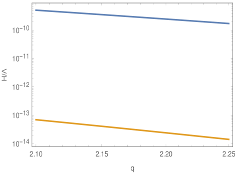
Figure 1: $H/\Lambda$ versus $q$ in the range $2.1\leq q\leq 2.25$, with $\lambda=1$, $\delta=0.1$, $H_{0}=10^{13}\mathrm{GeV}$ and $N_{\mathrm{f}}=51$. The blue curve represents the ratio of $\frac{H}{\Lambda}$ at the beginning of inflation when $H=H_{0}$, and the yellow curve specifies $\frac{H}{\Lambda}$ at the end of inflation when $H=H_{0}\exp{\left[-\left(\frac{\delta}{\delta+1}\right)N_{\mathrm{f}}\right]}$.

IV Constraint from perturbative requirement

In this section, we derive a bound on the parameter space of the conformal breaking coupling function $f(R,\mathcal{G})$ such that the theory can be treated perturbatively, and the perturbative QFT makes sense. If we expand the metric as $g_{\mu\nu}=\overline{g}_{\mu\nu}+\kappa h_{\mu\nu}$, where $\overline{g}_{\mu\nu}$ is the background FRW metric and $h_{\mu\nu}$ are the metric perturbations, then the conformal breaking action $S_{\mathrm{CB}}$ of Eq.(10) introduces non-minimal interaction terms between the graviton and photon. Such interaction Lagrangian is obtained in Eq.(28) as,

$$\frac{1}{\sqrt{-\overline{g}}}\mathcal{L}_{\mathrm{int}}\left[h_{\mu\nu},A_{\alpha}\right]=\lambda\kappa^{2q}\left\{\frac{\kappa}{2}\left(\overline{R}^{q}+\overline{\mathcal{G}}^{q/2}\right)h^{\mu}_{\mu}+q\left(\frac{\delta R}{\overline{R}^{1-q}}+\frac{\delta\mathcal{G}}{2\overline{\mathcal{G}}^{1-q/2}}\right)\right\}F_{\alpha\beta}\widetilde{F}^{\alpha\beta}~{}~{},$$ (36)

where $\delta R$ and $\delta\mathcal{G}$ are obtained in Eq.(25) and Eq.(26) respectively. The above interaction terms contribute in the Feynman-Dyson series of the 2-point correlator of EM field, and from the perturbative requirement, we demand that the first terms in the Feynman-Dyson series to be small. In particular, the constraint on the coupling function from perturbative requirement can be derived by either of the following two conditions:

1. the ratio of the actions for the conformal breaking term to the canonical electromagnetic term should be less than unity Durrer:2010mq , i.e,

   $$\left|\frac{S_{\mathrm{CB}}}{S_{\mathrm{em}}^{(can)}}\right|<1~{}~{}.$$ (37)

2. The loop contribution in the EM field propagator should be less than that of the tree propagator Ferreira:2015omg . In particular,

   $$\left|\frac{\big{\langle}AA\big{\rangle}_{1-loop}}{\big{\langle}AA\big{\rangle}_{tree}}\right|<1~{}~{},$$ (38)

   where $\big{\langle}AA\big{\rangle}_{tree}$ represents the tree propagator of the EM field and $\big{\langle}AA\big{\rangle}_{1-loop}$ indicates the loop correction in the EM 2-point correlator.

Here we would like to mention that these two conditions are equivalent, as the loop contribution in the EM propagator arises due to the presence of the action $S_{\mathrm{CB}}$.

To examine the first condition in the present context, we start with the following expression of the canonical EM Lagrangian,

$$-\frac{1}{4}F_{\mu\nu}F^{\mu\nu}=\frac{1}{a^{4}}\left(-\frac{1}{2}\left(A_{i}^{\prime}\right)^{2}+\frac{1}{4}F_{ij}F_{ij}\right)=\rho(\vec{E})-\rho(\vec{B})~{}~{},$$ (39)

where $\rho(\vec{E})$ and $\rho(\vec{B})$ are the electric and the magnetic energy density respectively. Consequently, the canonical EM action takes the following form,

$$S_{\mathrm{em}}^{(can)} = \int d\eta d^{3}x~{}a^{4}\big{(}\rho(\vec{E})-\rho(\vec{B})\big{)}$$ (40)

$$= V\int d\eta~{}a^{4}\bigg{(}\big{\langle}\rho(\vec{E})\big{\rangle}_{V}-\big{\langle}\rho(\vec{B})\big{\rangle}_{V}\bigg{)}~{}~{},$$

with $\big{\langle}...\big{\rangle}_{V}$ denotes the average over a spatial volume $V$ and is considered to be equivalent to the vacuum expectation value over the Bunch-Davies state (defined in Eq.(20) or in Eq.(21)). In particular,

$$a^{4}\big{\langle}\rho(\vec{E})\big{\rangle}_{V} = \sum_{r=1,2}\int\frac{k^{2}}{2\pi^{2}}\big{|}A_{r}^{\prime}(k,\eta)\big{|}^{2}~{}dk~{}~{},$$

$$a^{4}\big{\langle}\rho(\vec{B})\big{\rangle}_{V} = \sum_{r=1,2}\int\frac{k^{4}}{2\pi^{2}}\big{|}A_{r}(k,\eta)\big{|}^{2}~{}dk~{}~{}.$$ (41)

For the purpose of determining the $S_{\mathrm{CB}}$, we express $\epsilon^{\mu\nu\alpha\beta}F_{\mu\nu}F_{\alpha\beta}=F\widetilde{F}$, in the language of differential forms, as,

$$\sqrt{-g}F\widetilde{F}d^{4}x=4F\wedge F~{}~{}~{}~{}~{}~{}~{}~{}~{}~{}~{}~{}~{}~{}\mathrm{and}~{}~{}~{}~{}~{}~{}~{}~{}~{}~{}~{}~{}~{}~{}~{}F=dA~{}~{}.$$ (42)

Therefore the conformal breaking action turns out to be,

$$S_{\mathrm{CB}}=4\int\lambda f(R,\mathcal{G})\big{(}dA\wedge F\big{)}=4\int\lambda\big{(}df\wedge F\wedge A\big{)}~{}~{}.$$ (43)

To arrive at the second equality of the above expression, we use the integration by parts. Considering the comoving observer (having four velocity $u^{\mu}=\left(a^{-1},0,0,0\right)$ or $u=-ad\eta$) for measuring the electric and magnetic fields, we find $df\wedge F\wedge A=2f^{\prime}(\eta)a^{3}\rho_{h}$ (with $\rho_{h}$ being the helicity density) Durrer:2010mq . Accordingly the $S_{\mathrm{CB}}$ becomes,

$$S_{\mathrm{CB}}=8\int d\eta d^{3}x~{}\lambda f^{\prime}(\eta)\big{(}a^{3}\rho_{h}\big{)}=8\int d\eta~{}\lambda f^{\prime}(\eta)~{}a^{3}\big{\langle}\rho_{h}\big{\rangle}_{V}~{}~{},$$ (44)

where $\big{\langle}\rho_{h}\big{\rangle}_{V}$ is given by,

$$a^{3}\big{\langle}\rho_{h}\big{\rangle}_{V}=\int\frac{k^{3}}{2\pi^{2}}\left\{\big{|}A_{+}(k,\eta)\big{|}^{2}-\big{|}A_{-}(k,\eta)\big{|}^{2}\right\}dk~{}~{}.$$ (45)

Plugging back the above expressions into the left hand side of Eq.(37), we arrive at the following equation,

$$\left|\frac{S_{\mathrm{CB}}}{S_{\mathrm{em}}^{(can)}}\right| = \left|\frac{8\int d\eta~{}\lambda f^{\prime}(\eta)~{}a^{3}\big{\langle}\rho_{h}\big{\rangle}_{V}}{\int d\eta~{}a^{4}\bigg{(}\big{\langle}\rho(\vec{E})\big{\rangle}_{V}-\big{\langle}\rho(\vec{B})\big{\rangle}_{V}\bigg{)}}\right|~{}.$$ (46)

Now, for the condition $\left|\frac{S_{\mathrm{CB}}}{S_{\mathrm{em}}^{(can)}}\right|<1$ to be satisfied, it is sufficient to require

$$\frac{8\lambda f^{\prime}(\eta)~{}a^{3}\big{\langle}\rho_{h}\big{\rangle}_{V}}{a^{4}\left(\big{\langle}\rho(\vec{E})\big{\rangle}_{V}-\big{\langle}\rho(\vec{B})\big{\rangle}_{V}\right)}<1~{}~{}.$$ (47)

Let us denote the ratio in the left hand side of Eq.(47) by $\mathcal{Z}$. Eq.(12) immediately leads to $f^{\prime}(\eta)$ as,

$$f^{\prime}(\eta)=\frac{1}{8\lambda}\left(\frac{\zeta^{2}}{\eta^{2}}\right)\left(\frac{-\eta_{0}}{\eta}\right)^{2\alpha}~{}~{},$$ (48)

where $\zeta^{2}$ is given in Eq.(17), due to which, $\mathcal{Z}$ can be equivalently expressed as,

$$\mathcal{Z}=H_{0}\left(16\epsilon q\lambda\right)\left(\frac{H_{0}}{M_{\mathrm{Pl}}}\right)^{2q}\left\{\big{[}6\beta(\beta+1)\big{]}^{q}+\big{[}-24(\beta+1)^{3}\big{]}^{q/2}\right\}\left(\frac{-\eta_{0}}{\eta}\right)^{1+2\alpha}\left[\frac{\big{\langle}\rho_{h}\big{\rangle}_{V}}{\left(\big{\langle}\rho(\vec{E})\big{\rangle}_{V}-\big{\langle}\rho(\vec{B})\big{\rangle}_{V}\right)}\right]~{}~{}.$$ (49)

Moreover from Eq.(20), Eq.(21) and Eq.(22), we have the following expressions,

$$\big{\langle}\rho(\vec{E},\eta_{c})\big{\rangle}_{V} = \int_{k_{i}}^{k_{c}}\frac{dk}{2\pi^{4}}\left(\frac{H_{0}}{k}\right)^{2}H^{4+4\delta}\left(-k\eta\right)^{4+4\delta}\left|\left(\frac{\zeta\sqrt{k}}{2\alpha}\right)^{-\frac{1}{2\alpha}}\Gamma\left(\frac{1}{2\alpha}\right)\right|^{2}\left\{\left|C_{2}\right|^{2}\right\}~{}~{},$$

$$\big{\langle}\rho(\vec{B},\eta_{c})\big{\rangle}_{V} = \int_{k_{i}}^{k_{c}}\frac{dk}{2\pi^{2}}H^{4+\delta}\left(-k\eta\right)^{4+\delta}\left|\frac{\left(\frac{\zeta\sqrt{k}}{2\alpha}\right)^{\frac{1}{2\alpha}}}{\Gamma\left(1+\frac{1}{2\alpha}\right)}\right|^{2}\left\{\left|C_{1}-C_{2}\cot{\left(-\frac{\pi}{2\alpha}\right)}\right|^{2}\right\}~{}~{},$$

$$\big{\langle}\rho_{h}(\eta_{c})\big{\rangle}_{V} = \int_{k_{i}}^{k_{c}}\frac{dk}{2\pi^{2}}H^{3+3\delta}\left(-k\eta\right)^{3+3\delta}\left|\frac{\left(\frac{\zeta\sqrt{k}}{2\alpha}\right)^{1/(2\alpha)}}{\Gamma\left(1+\frac{1}{2\alpha}\right)}\right|^{2}\left\{\left|C_{1}-C_{2}\cot{\left(-\frac{\pi}{2\alpha}\right)}\right|^{2}\right\}~{}~{},$$ (50)

respectively, where $C_{i}$ ($i=1,2,3,4$) are shown in the Appendix. The integration limit in Eq.(50) is taken from $k_{i}$ to $k_{c}$, i.e from the mode that crosses the horizon at the beginning of inflation to the mode which crosses the horizon at the instance $\eta=\eta_{c}$. Now we identify the beginning of inflation when the horizon is of same size with the CMB scale mode, i.e we may write $k_{i}=k_{CMB}=0.05\mathrm{Mpc}^{-1}$. Furthermore we have $|k_{c}\eta_{c}|=1$ with $\eta_{c}$ is any time during the inflation and thus $k_{c}>k_{CMB}$. The quantity $N_{\mathrm{c}}$ is the e-folding number up-to $\eta=\eta_{c}$ measured from the beginning of inflation, i.e $N_{\mathrm{c}}=\ln{\left(\frac{a_{c}}{a_{beg}}\right)}$ with $a_{c}=a(\eta_{c})$ and $a_{beg}=a(\eta_{beg})$. Having obtained the necessary ingredients, we now examine whether the condition $\mathcal{Z}<1$ is satisfied during inflation. However due to the dependence of $C_{i}=C_{i}(k)$ ($i=1,2,3,4$), the integrations in Eq.(50) may not be obtained in analytic form(s), and thus we numerically approach to integrate $\big{\langle}\rho(\vec{E})\big{\rangle}_{V}$, $\big{\langle}\rho(\vec{B})\big{\rangle}_{V}$ and $\big{\langle}\rho_{h}\big{\rangle}_{V}$ (at $\eta_{c}$) present in Eq.(50). For this purpose, we consider $H_{0}=10^{13}\mathrm{GeV}$, $N_{\mathrm{f}}=51$ and $\delta=0.1$ respectively, and perform the numerical integrations of Eq.(50). Consequently we depict the plot of $\mathcal{Z}$ with respect to the parameter $q$ in the range $2.1\leq q\leq 2.25$, see Fig.[2]. Recall this range of $q$ results to the correct magnetic strength at present epoch of the universe, and thus we are using such range of $q$ to examine the perturbative condition in order to keep intact the generation of the EM field. We consider different values of $k_{c}$ in Fig.[2], in particular, we consider $k_{c}=10^{-20}\mathrm{GeV}$ and $10^{-38}\mathrm{GeV}$ in the left and right plot of Fig.[2] respectively. Here we would like to mention that the mode $k_{c}=10^{-20}\mathrm{GeV}$ crosses the horizon near the end of inflation, i.e $N_{c}\approx N_{f}$; while the mode $k_{c}=10^{-38}\mathrm{GeV}$ crosses the horizon near $N_{c}\approx 3$ i.e near the beginning of inflation.

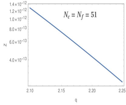
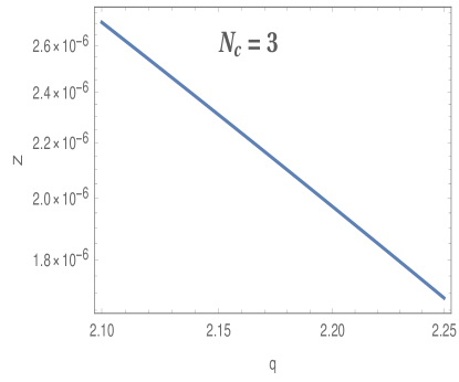
Figure 2: $\mathcal{Z}$ vs $q$ for $H_{0}=10^{13}\mathrm{GeV}$, $N_{\mathrm{f}}=51$ and $\delta=0.1$. Moreover we take $\lambda=1$. In the left plot, $k_{c}=10^{-20}\mathrm{GeV}$ that crosses the horizon near the end of inflation, i.e $N_{\mathrm{c}}\approx N_{\mathrm{f}}=51$; while for the right plot, $k_{c}=10^{-38}\mathrm{GeV}$ which crosses the horizon near $N_{c}\approx 3$ i.e near the beginning of inflation.

The Fig.[2] clearly demonstrates that the perturbative condition $\mathcal{Z}<1$ is satisfied for $q=[2.1,2.25]$ which also leads to the viability of the model in regard to the CMB observations of current magnetic strength. Therefore the predictions of perturbative QFT in the model are found to be consistent with the observational bound of the model parameter required to get sufficient magnetic strength at current stage of the universe.

V Curvature perturbation sourced by electromagnetic field during inflation

The produced electromagnetic field during inflation may induce the curvature perturbation Fujita:2013qxa ; Barnaby:2012tk ; Bamba:2014vda ; Suyama:2012wh , and the power spectrum of the induced curvature perturbations should satisfy the recent Planck constraints. Thereby in the present magnetogenesis scenario where the electromagnetic field couples with the background curvature terms via the dual field tensor, it is important to examine the viability of the sourced curvature perturbations in respect to the Planck constraints.

The induced curvature perturbation (symbolized by $\chi(\eta,\vec{x})$) from the electromagnetic field is expressed as Fujita:2013qxa ,

$$\chi_{em}(\eta,\vec{x})=-\frac{2H}{\epsilon\rho_{inf}}\int_{\eta_{m}}^{\eta}d\eta^{\prime}~{}a(\eta^{\prime})\rho_{em}(\eta^{\prime},\vec{x})$$ (51)

where $\rho_{inf}$ is the background inflaton energy density and $\rho_{em}$ denotes the EM field energy density. Here it may be mentioned that the contribution from the electromagnetic anisotropic stress is suppressed compared to the contribution written in the r.h.s of Eq.(51) (see Suyama:2012wh ), and thus the electromagnetic anisotropic stress in the curvature perturbation is not taken into account in Eq.(51). The lower limit of the integral, i.e $\eta_{m}$, represents the time at which the EM production effectively starts.

The EM energy density can be expressed by $\rho_{em}(\eta,\vec{x})=\rho_{E}(\eta,\vec{x})+\rho_{B}(\eta,\vec{x})$, where $\rho_{E}(\eta,\vec{x})$ and $\rho_{B}(\eta,\vec{x})$ are the energy density for electric and magnetic fields respectively. However from Eq.(20) and Eq.(21), the ratio of electric to magnetic power spectrum during inflation comes as $\frac{\mathcal{P}(\vec{E})}{\mathcal{P}(\vec{B})}\sim 10^{5}$. In particular, we give the plot of $\frac{\mathcal{P}(\vec{E})}{\mathcal{P}(\vec{B})}$ with respect to $q$ in the range $2.1\leq q\leq 2.25$ on which we are interested, see Fig.[3].

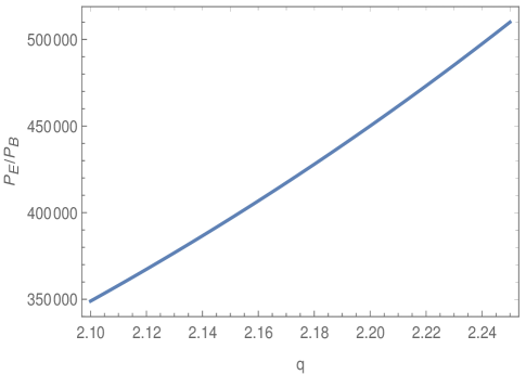
Figure 3: $\frac{\mathcal{P}(\vec{E})}{\mathcal{P}(\vec{B})}$ vs $q$ in the range $2.1\leq q\leq 2.25$. Here we consider $H_{0}=10^{13}\mathrm{GeV}$, $N_{\mathrm{f}}=51$ and $\delta=0.1$. Moreover we take $\lambda=1$.

The figure clearly depicts that the electric field during inflation is $\sim 10^{5}$ times stronger than that of the magnetic field strength. This in turn indicates that the main contribution of the EM energy density comes from the electric field, and thus we may write $\rho_{em}\approx\rho_{E}=\frac{1}{2}E^{2}$. Consequently the EM field energy density in Fourier space is given by,

$$\rho_{em}(\eta_{\mathrm{f}},\vec{k})=\frac{1}{2}\int\int\frac{d^{3}p_{1}d^{3}p_{2}}{(2\pi)^{3}}~{}\delta\big{(}\vec{p}_{1}+\vec{p}_{2}-\vec{k}\big{)}\vec{E}(\eta_{\mathrm{f}},\vec{p}_{1})\vec{E}(\eta_{\mathrm{f}},\vec{p}_{2})~{}~{},$$ (52)

where the electric field is defined as $\big{|}E(\eta,k)\big{|}=\frac{1}{a^{2}}\big{|}A^{\prime}(k,\eta)\big{|}$ with respect to the comoving observer. Thereby Eq.(19) immediately leads to the electric field as,

$$\big{|}E(\eta,k)\big{|}=k\left(\frac{H_{0}}{k}\right)\left|\left(\frac{C_{2}\Gamma\left(\frac{1}{2\alpha}\right)}{\pi}\right)\left(\frac{\zeta\sqrt{k}}{2\alpha}\right)^{-1/(2\alpha)}\right|\left(-H\eta\right)^{2}~{}~{}.$$ (53)

With the above expression of $\big{|}E(\eta,k)\big{|}$, we evaluate the 2-point correlator of $\zeta_{em}(\eta,\vec{k})$ in the present context as Fujita:2013qxa ,

$$\langle\chi_{em}(\eta_{f},\vec{k}_{1})\chi_{em}(\eta_{f},\vec{k}_{2})\rangle = 2\delta\big{(}\vec{k}_{1}+\vec{k}_{2}\big{)}G_{2}\int_{k_{CMB}}^{k_{f}}d^{3}p_{1}d^{3}p_{2}\delta\left(\vec{p}_{2}-\vec{p}_{1}-\vec{k}_{2}\right)\left[f(p_{1})f(p_{2})\right]^{2}$$ (54)

$$\times \left(\delta_{j_{1}j_{2}}-\big{(}\hat{p}_{1}\big{)}_{j_{1}}\big{(}\hat{p}_{1}\big{)}_{j_{2}}\right)\left(\delta_{j_{1}j_{2}}-\big{(}\hat{p}_{2}\big{)}_{j_{1}}\big{(}\hat{p}_{2}\big{)}_{j_{2}}\right)\bigg{\{}\prod_{i=1,2}~{}\int_{\eta_{m}}^{\eta_{f}}d\eta_{i}\big{(}-\eta_{i}\big{)}^{3+3\delta}\bigg{\}}$$

where $G_{2}$ and $f(p)$ have the following forms,

$$G_{2}=\bigg{[}\frac{H_{f}^{2}}{6\epsilon M_{\mathrm{Pl}}^{2}}\bigg{]}^{2}~{}~{},$$ (55)

and

$$f(k)=k\left(\frac{H_{0}}{k}\right)\left|\left(\frac{C_{2}\Gamma\left(\frac{1}{2\alpha}\right)}{\pi}\right)\left(\frac{\zeta\sqrt{k}}{2\alpha}\right)^{-1/(2\alpha)}\right|~{}~{},$$ (56)

respectively. Here $k_{\mathrm{f}}$ in Eq.(54) symbolizes the mode that crosses the horizon at the end of inflation. Moreover, to derive $G_{2}$, we use $\rho_{inf}(\eta_{f})=3H_{f}^{2}M_{\mathrm{Pl}}^{2}$. Such expression of $\rho_{inf}$ holds true as the EM field provides a negligible backreaction on the background spacetime in the present magnetogenesis scenario. We may perform the $p_{2}$ integral of Eq.(54), to get

$$\langle\chi_{em}(\eta_{f},\vec{k}_{1})\chi_{em}(\eta_{f},\vec{k}_{2})\rangle=\frac{32\pi}{3}\delta\big{(}\vec{k}_{1}+\vec{k}_{2}\big{)}G_{2}\int_{k_{CMB}}^{k_{f}}dp_{1}~{}p_{1}^{2}~{}\left[f(p_{1})f(p_{1}+k_{2})\right]^{2}\bigg{\{}\prod_{i=1,2}~{}\int_{-1/p_{1}}^{\eta_{f}}d\eta_{i}\big{(}-\eta_{i}\big{)}^{3+3\delta}\bigg{\}}~{}.$$ (57)

where we use the integral $\int d\Omega_{k}\hat{k}_{i}\hat{k}_{j}=\frac{4\pi}{3}\delta_{ij}$. For the momentum variable $p_{1}$ in the above integral, the corresponding lower limit of the $\eta$ integral is taken as

$$\eta_{m}=-\frac{1}{p_{1}}~{}~{},$$ (58)

i.e when the mode $p_{1}$ crosses the horizon. This is due to the reason that the EM fluctuations of momentum $p_{1}$ starts to effectively produce from the horizon crossing of $p_{1}$. In particular, the energy density stored in a certain mode of the gauge field is maximal (compared to the background energy density) at horizon crossing of the corresponding mode and then redshifts almost like radiation. Therefore a certain EM mode is mainly produced near the horizon crossing of that mode in the present magnetogenesis scenario. The consideration of $\eta_{m}=-1/p_{1}$ indeed takes care the horizon crossing region of the mode variable $p_{1}$. With $\eta_{m}=-1/p_{1}$ and $\eta_{f}=-1/k_{f}$, we evaluate the $\eta$ integral of Eq.(57), and get

$$\langle\chi_{em}(\eta_{f},\vec{k}_{1})\chi_{em}(\eta_{f},\vec{k}_{2})\rangle=\frac{32\pi}{3}\delta\big{(}\vec{k}_{1}+\vec{k}_{2}\big{)}G_{2}\int_{k_{CMB}}^{k_{f}}dp_{1}~{}p_{1}^{2}~{}\left[f(p_{1})f(p_{1}+k_{2})\right]^{2}\bigg{\{}\frac{\left(1/p_{1}\right)^{4+3\delta}-\left(1/k_{f}\right)^{4+3\delta}}{4+3\delta}\bigg{\}}^{2}~{}.$$ (59)

We will eventually evaluate the two point correlator at CMB scale, and thus $k_{1}=k_{2}=k_{CMB}$. The above expression of 2-point correlator yields the power spectrum of the curvature perturbation (at $k=k_{1}$) induced by the EM field as,

$$\mathcal{P}(\chi_{em},k_{1})=G_{2}\left(\frac{16}{3\pi}\right)k_{1}^{3}\int_{k_{1}}^{k_{f}}dp_{1}~{}p_{1}^{2}~{}\left[f(p_{1})f(p_{1}+k_{2})\right]^{2}\bigg{\{}\frac{\left(1/p_{1}\right)^{4+3\delta}-\left(1/k_{f}\right)^{4+3\delta}}{4+3\delta}\bigg{\}}^{2}~{}~{},$$ (60)

where the functional form of $f(p_{1})$ or $f(p_{1}+k_{2})$ are shown in Eq.(56).

Having obtained the theoretical expression of induced power spectrum in hand, we now confront the model with the Planck results which put constraint on curvature perturbation as,

$$\mathcal{P}^{obs}(\chi)\approx 2.1\times 10^{-9}~{}~{}.$$ (61)

We consider that the dominant component of the power spectrum of the curvature perturbation is generated by the background slow-roll inflaton field. As a consequence, the theoretical prediction of $\mathcal{P}(\chi_{em})$ does not exceed the aforementioned Planck constraint, in particular,

$$\mathcal{P}(\chi_{em})<\mathcal{P}^{obs}(\chi)~{}~{}.$$ (62)

In order to investigate $\mathcal{P}(\chi_{em})<\mathcal{P}^{obs}(\chi)$ in the present context, we need to evaluate the $p_{1}$ integral of Eq.(60). However due to the aforementioned form of $f(k)$, this integral may not be obtained in a closed form, so we perform the integration by numerical analysis. This is depicted in Fig.[4] where we take the following set of parameters: $H_{0}=10^{13}\mathrm{GeV}$, $\delta=0.1$, $N_{\mathrm{f}}=51$ and $\lambda=1$. In particular, we plot the ratio of $\frac{\mathcal{P}(\chi_{em})}{\mathcal{P}^{obs}(\chi)}$ with respect to the parameter $q$ in Fig.[4].

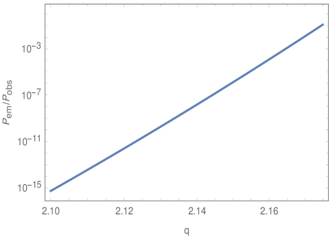
Figure 4: $\frac{\mathcal{P}(\chi_{em})}{\mathcal{P}^{obs}(\chi)}$ vs $q$. Here we consider $H_{0}=10^{13}\mathrm{GeV}$, $N_{f}=51$ and $\delta=0.1$. Moreover we take $\lambda=1$.

The Fig.[4] clearly demonstrates that in order to satisfy $\mathcal{P}(\chi_{em})<\mathcal{P}^{obs}(\chi)$, the parameter $q$ should lie within $q\lesssim 2.175$. Moreover we recall that the magnetogenesis model under consideration predicts correct magnetic strength at present universe for $2.1\lesssim q\lesssim 2.25$. Therefore it turns out that the whole range of $q$ which gives the correct magnetic strength, does not obey the condition of the induced curvature perturbation i.e $\mathcal{P}(\chi_{em})<\mathcal{P}^{obs}(\chi)$. In particular, the range of $q$ which leads to a sufficient magnetic strength at present universe and also ensures $\mathcal{P}(\chi_{em})<\mathcal{P}^{obs}(\chi)$, is given by: $2.1\lesssim q\lesssim 2.175$.

Before concluding we would like to mention that some recent literatures have argued that non-linear enhancement of the magnetic fields at the end of inflation, inverse cascade of helical photons after inflation and/or a simultaneous coupling to the photon kinetic term $F_{\mu\nu}F^{\mu\nu}$ could help increase the strength of the magnetic field Adshead:2016iae ; Fujita:2019pmi . Such considerations in the present curvature coupled helical magnetogenesis scenario will be examined in future work.

VI Conclusion

The recently proposed curvature coupling helical magnetogenesis scenario Bamba:2021wyx , where the EM field couples with the background $f(R,\mathcal{G})$ gravity, has the following strong features – (1) the model predicts sufficient magnetic strength at current epoch of the universe for suitable range of the model parameter ($q$) given by: $2.1\leq q\leq 2.26$ for instantaneous reheating scenario and $2.1\leq q\leq 2.25$ for Kamionkowski reheating scenario respectively; (2) the EM field is found to have a negligible backreaction over the background spacetime and does not jeopardize the background inflation; (3) the model is free from the strong couping problem; (4) due to the helical nature of the magnetic field, it turns out that the magnetic strength of $\sim 10^{-13}\mathrm{G}$ over the galactic scale results to the correct baryon asymmetry of the universe consistent with the observational data.

However in the realm of inflationary magnetogenesis, the above requirements are not enough to argue about the viability of the model. In particular, one needs to examine some more important requirements to ensure the viability of a magnetogenesis model, such as – (1) whether the model is consistent with the predictions of perturbative QFT, as the calculations that we use to determine the magnetic field’s evolution and its power spectrum are based on the perturbative QFT; (2) the curvature perturbation sourced by the EM field during inflation should not exceed than the curvature perturbation contributed from the background inflaton field, in order to be consistent with the recent Planck data; and (3) the relevant energy scale of the magnetogenesis model needs to be lie below than the cut-off scale of the model. We have checked all these requirements in the present context of curvature coupling helical magnetogenesis scenario. For the perturbative requirement, we have examined whether the condition $\left|\frac{S_{CB}}{S_{can}}\right|<1$ is satisfied, where $S_{can}$ and $S_{CB}$ are the canonical and the conformal breaking action of the EM field respectively. The condition $\left|\frac{S_{CB}}{S_{can}}\right|<1$ actually indicates that the loop contribution of EM two-point correlator is less than the tree propagator of the EM field – which is the essence of the perturbative quantum field theory. For the second requirement, we have calculated the power spectrum of curvature perturbation sourced by the EM field at super-Hubble scales ($\mathcal{P}(\chi_{em})$). By considering that the primordial curvature perturbation is mainly contributed from the slow-roll inflaton field, we have determined the necessary condition corresponding to the requirement given by: $\mathcal{P}(\chi_{em})<\mathcal{P}^{obs}(\chi)$, where $\mathcal{P}^{obs}(\chi)$ corresponds to the Planck observation of the curvature perturbation power spectrum. This puts a constraint on the parameter $q$ as $q\lesssim 2.175$. Therefore it turns out that the whole range of $q$ which gives the correct magnetic strength, does not obey the condition of the induced curvature perturbation i.e $\mathcal{P}(\chi_{em})<\mathcal{P}^{obs}(\chi)$. In particular, the range of $q$ which leads to a sufficient magnetic strength at present universe and also ensures $\mathcal{P}(\chi_{em})<\mathcal{P}^{obs}(\chi)$, is given by: $2.1\lesssim q\lesssim 2.175$.

Interestingly, all the three aforementioned requirements are found to be simultaneously satisfied by that range of the model parameter which leads to the correct magnetic strength over the large scale modes.

VII Appendix: Forms of $C_{i}$ ($i=1,2,3,4$)

The solutions of $A_{\pm}(k,\eta)$ can be demonstrated as follows: in the sub-Hubble scale when $k>\mathcal{H}$, the EM mode functions remain in Bunch-Davies vacuum state; and in the super-Hubble scale when $k<\mathcal{H}$, the $A_{\pm}(k,\eta)$ are given by Eq.(18). Here $C_{i}$ are the integration constants which can be determined by matching $A_{\pm}(k,\eta)$ and $A_{\pm}^{\prime}(k,\eta)$ at the transition time of sub-Hubble and super-Hubble regimes, i.e when $k=\mathcal{H}$. If $\eta_{*}$ is the horizon crossing instance of the mode $k$, then we have $k\eta_{*}=-(1+\delta)$, where $\delta$ is shown in Eq.(5). As a result, the $C_{i}$ are given by the following expressions Bamba:2021wyx ,

$$C_{1} = \frac{-1}{2\alpha\sqrt{-2k\eta_{*}/\eta_{0}}}\left[i\pi e^{-ik\eta_{*}}\left\{-\zeta\sqrt{k}\tau_{*}~{}Y_{1+\frac{1}{2\alpha}}\left(-i\frac{\zeta\sqrt{k}}{\alpha}\tau_{*}\right)+k\eta_{*}~{}Y_{\frac{1}{2\alpha}}\left(-i\frac{\zeta\sqrt{k}}{\alpha}\tau_{*}\right)\right\}\right]~{}~{},$$

$$C_{2} = \frac{-1}{4\alpha\sqrt{-2k\eta_{*}/\eta_{0}}}\bigg{[}i\pi e^{-ik\eta_{*}}\bigg{\{}-\zeta\sqrt{k}\tau_{*}\left(J_{-1+\frac{1}{2\alpha}}\left(-i\frac{\zeta\sqrt{k}}{\alpha}\tau_{*}\right)-J_{1+\frac{1}{2\alpha}}\left(-i\frac{\zeta\sqrt{k}}{\alpha}\tau_{*}\right)\right)$$ (63)

$$+ \left(i-2k\eta_{*}\right)~{}J_{\frac{1}{2\alpha}}\left(-i\frac{\zeta\sqrt{k}}{\alpha}\tau_{*}\right)\bigg{\}}\bigg{]}~{}~{}.$$

Similarly,

$$C_{3} = \frac{-1}{2\alpha\sqrt{-2k\eta_{*}/\eta_{0}}}\left[-\pi e^{-ik\eta_{*}}\left\{-\zeta\sqrt{k}\tau_{*}~{}Y_{1+\frac{1}{2\alpha}}\left(\frac{\zeta\sqrt{k}}{\alpha}\tau_{*}\right)-ik\eta_{*}~{}Y_{\frac{1}{2\alpha}}\left(\frac{\zeta\sqrt{k}}{\alpha}\tau_{*}\right)\right\}\right]~{}~{},$$

$$C_{4} = \frac{-1}{2\alpha\sqrt{-2k\eta_{*}/\eta_{0}}}\left[\pi e^{-ik\eta_{*}}\left\{-\zeta\sqrt{k}\tau_{*}~{}J_{1+\frac{1}{2\alpha}}\left(\frac{\zeta\sqrt{k}}{\alpha}\tau_{*}\right)-ik\eta_{*}~{}J_{\frac{1}{2\alpha}}\left(\frac{\zeta\sqrt{k}}{\alpha}\tau_{*}\right)\right\}\right]~{}.$$ (64)

In the above expressions, $\tau_{*}=\left(-\eta_{0}/\eta_{*}\right)^{\alpha}$ and $\alpha$, $\zeta^{2}$ are shown earlier in Eq.(17).

Acknowledgments

TP sincerely acknowledges Sergei D. Odintsov for useful discussions. This research was supported in part by the International Centre for Theoretical Sciences (ICTS) for the online program - Physics of the Early Universe: ICTS/peu2022/1.

References

- (1) K. Bamba, S. D. Odintsov, T. Paul and D. Maity, Phys. Dark Univ. 36 (2022), 101025 doi:10.1016/j.dark.2022.101025 [arXiv:2107.11524 [gr-qc]].
- (2) D. Grasso and H. R. Rubinstein, Phys. Rept. 348 (2001), 163-266 [arXiv:astro-ph/0009061 [astro-ph]].
- (3) R. Beck, Space Sci. Rev. 99 (2001), 243-260 [arXiv:astro-ph/0012402 [astro-ph]].
- (4) L. M. Widrow, Rev. Mod. Phys. 74 (2002), 775-823 [arXiv:astro-ph/0207240 [astro-ph]].
- (5) R. M. Kulsrud and E. G. Zweibel, Rept. Prog. Phys. 71 (2008), 0046091 [arXiv:0707.2783 [astro-ph]].
- (6) A. Brandenburg and K. Subramanian, Phys. Rept. 417 (2005), 1-209 [arXiv:astro-ph/0405052 [astro-ph]].
- (7) K. Subramanian, Astron. Nachr. 331 (2010), 110-120 [arXiv:0911.4771 [astro-ph.CO]].
- (8) R. K. Jain and M. S. Sloth, Phys. Rev. D 86 (2012), 123528 [arXiv:1207.4187 [astro-ph.CO]].
- (9) R. Durrer, L. Hollenstein and R. K. Jain, JCAP 03 (2011), 037 [arXiv:1005.5322 [astro-ph.CO]].
- (10) S. Kanno, J. Soda and M. a. Watanabe, JCAP 12 (2009), 009 [arXiv:0908.3509 [astro-ph.CO]].
- (11) L. Campanelli, Int. J. Mod. Phys. D 18 (2009), 1395-1411 [arXiv:0805.0575 [astro-ph]].
- (12) V. Demozzi, V. Mukhanov and H. Rubinstein, JCAP 08 (2009), 025 [arXiv:0907.1030 [astro-ph.CO]].
- (13) V. Demozzi and C. Ringeval, JCAP 05, 009 (2012) [arXiv:1202.3022 [astro-ph.CO]].
- (14) K. Bamba and M. Sasaki, JCAP 02 (2007), 030 [arXiv:astro-ph/0611701 [astro-ph]].
- (15) T. Kobayashi and M. S. Sloth, Phys. Rev. D 100 (2019) no.2, 023524 [arXiv:1903.02561 [astro-ph.CO]].
- (16) K. Bamba, E. Elizalde, S. D. Odintsov and T. Paul, JCAP 04 (2021), 009 doi:10.1088/1475-7516/2021/04/009 [arXiv:2012.12742 [gr-qc]].
- (17) D. Maity, S. Pal and T. Paul, JCAP 05 (2021), 045 doi:10.1088/1475-7516/2021/05/045 [arXiv:2103.02411 [hep-th]].
- (18) M. R. Haque, D. Maity and S. Pal, [arXiv:2012.10859 [hep-th]].
- (19) B. Ratra, Astrophys. J. Lett. 391 (1992), L1-L4
- (20) P. A. R. Ade et al. [Planck], Astron. Astrophys. 594 (2016), A19 [arXiv:1502.01594 [astro-ph.CO]].
- (21) D. Chowdhury, L. Sriramkumar and M. Kamionkowski, JCAP 10 (2018), 031 [arXiv:1807.07477 [astro-ph.CO]].
- (22) M. S. Turner and L. M. Widrow, Phys. Rev. D 37 (1988), 2743
- (23) S. Tripathy, D. Chowdhury, R. K. Jain and L. Sriramkumar, Phys. Rev. D 105 (2022) no.6, 063519 doi:10.1103/PhysRevD.105.063519 [arXiv:2111.01478 [astro-ph.CO]].
- (24) R. J. Z. Ferreira, R. K. Jain and M. S. Sloth, JCAP 10 (2013), 004 [arXiv:1305.7151 [astro-ph.CO]].
- (25) K. Atmjeet, T. R. Seshadri and K. Subramanian, Phys. Rev. D 91 (2015), 103006 [arXiv:1409.6840 [astro-ph.CO]].
- (26) A. Kushwaha and S. Shankaranarayanan, Phys. Rev. D 102 (2020) no.10, 103528 doi:10.1103/PhysRevD.102.103528 [arXiv:2008.10825 [gr-qc]].
- (27) M. Gasperini, M. Giovannini and G. Veneziano, Phys. Rev. Lett. 75 (1995), 3796-3799 doi:10.1103/PhysRevLett.75.3796 [arXiv:hep-th/9504083 [hep-th]].
- (28) M. Giovannini, Phys. Rev. D 104 (2021) no.12, 123509 doi:10.1103/PhysRevD.104.123509 [arXiv:2106.14927 [hep-th]].
- (29) M. Giovannini, Eur. Phys. J. C 81 (2021) no.6, 503 doi:10.1140/epjc/s10052-021-09282-7 [arXiv:2103.04137 [astro-ph.CO]].
- (30) P. Adshead, J. T. Giblin, T. R. Scully and E. I. Sfakianakis, JCAP 12 (2015), 034 [arXiv:1502.06506 [astro-ph.CO]].
- (31) C. Caprini and L. Sorbo, JCAP 10 (2014), 056 [arXiv:1407.2809 [astro-ph.CO]].
- (32) T. Kobayashi, JCAP 05 (2014), 040 [arXiv:1403.5168 [astro-ph.CO]].
- (33) K. Atmjeet, I. Pahwa, T. R. Seshadri and K. Subramanian, Phys. Rev. D 89 (2014) no.6, 063002 [arXiv:1312.5815 [astro-ph.CO]].
- (34) T. Fujita, R. Namba, Y. Tada, N. Takeda and H. Tashiro, JCAP 05 (2015), 054 [arXiv:1503.05802 [astro-ph.CO]].
- (35) L. Campanelli, Eur. Phys. J. C 75 (2015) no.6, 278 [arXiv:1503.07415 [gr-qc]].
- (36) G. Tasinato, JCAP 03 (2015), 040 [arXiv:1411.2803 [hep-th]].
- (37) D. Nandi, JCAP 08 (2021), 039 doi:10.1088/1475-7516/2021/08/039 [arXiv:2103.03159 [astro-ph.CO]].
- (38) E. Frion, N. Pinto-Neto, S. D. P. Vitenti and S. E. Perez Bergliaffa, Phys. Rev. D 101 (2020) no.10, 103503 [arXiv:2004.07269 [gr-qc]].
- (39) R. Koley and S. Samtani, JCAP 04 (2017), 030 [arXiv:1612.08556 [gr-qc]].
- (40) P. Qian, Y. F. Cai, D. A. Easson and Z. K. Guo, Phys. Rev. D 94 (2016) no.8, 083524 [arXiv:1607.06578 [gr-qc]].
- (41) A.H. Guth; Phys.Rev. D23 347-356 (1981).
- (42) A. D. Linde, Contemp. Concepts Phys. 5 (1990) 1 [hep-th/0503203].
- (43) D. Langlois, hep-th/0405053.
- (44) A. Riotto, ICTP Lect. Notes Ser. 14 (2003) 317 [hep-ph/0210162].
- (45) D. Baumann, [arXiv:0907.5424 [hep-th]].
- (46) L. Dai, M. Kamionkowski and J. Wang, Phys. Rev. Lett. 113 (2014), 041302 [arXiv:1404.6704 [astro-ph.CO]].
- (47) J. L. Cook, E. Dimastrogiovanni, D. A. Easson and L. M. Krauss, JCAP 04 (2015), 047 [arXiv:1502.04673 [astro-ph.CO]].
- (48) A. Albrecht, P. J. Steinhardt, M. S. Turner and F. Wilczek, Phys. Rev. Lett. 48 (1982), 1437
- (49) J. Ellis, M. A. G. Garcia, D. V. Nanopoulos and K. A. Olive, JCAP 07 (2015), 050 [arXiv:1505.06986 [hep-ph]].
- (50) Y. Ueno and K. Yamamoto, Phys. Rev. D 93 (2016) no.8, 083524 [arXiv:1602.07427 [astro-ph.CO]].
- (51) M. Eshaghi, M. Zarei, N. Riazi and A. Kiasatpour, Phys. Rev. D 93 (2016) no.12, 123517 [arXiv:1602.07914 [astro-ph.CO]].
- (52) D. Maity and P. Saha, JCAP 07 (2019), 018 [arXiv:1811.11173 [astro-ph.CO]].
- (53) M. R. Haque, D. Maity, T. Paul and L. Sriramkumar, Phys. Rev. D 104 (2021) no.6, 063513 doi:10.1103/PhysRevD.104.063513 [arXiv:2105.09242 [astro-ph.CO]].
- (54) A. Di Marco, P. Cabella and N. Vittorio, Phys. Rev. D 95 (2017) no.10, 103502 [arXiv:1705.04622 [astro-ph.CO]].
- (55) M. Drewes, J. U. Kang and U. R. Mun, JHEP 11 (2017), 072 [arXiv:1708.01197 [astro-ph.CO]].
- (56) S. Nojiri, S. D. Odintsov and M. Sasaki, Phys. Rev. D 71 (2005), 123509 doi:10.1103/PhysRevD.71.123509 [arXiv:hep-th/0504052 [hep-th]].
- (57) B. Li, J. D. Barrow and D. F. Mota, Phys. Rev. D 76 (2007), 044027 doi:10.1103/PhysRevD.76.044027 [arXiv:0705.3795 [gr-qc]].
- (58) B. M. Carter and I. P. Neupane, JCAP 06 (2006), 004 doi:10.1088/1475-7516/2006/06/004 [arXiv:hep-th/0512262 [hep-th]].
- (59) S. Nojiri, S. Odintsov, V. Oikonomou, N. Chatzarakis and T. Paul, Eur. Phys. J. C 79 (2019) no.7, 565 doi:10.1140/epjc/s10052-019-7080-1 [arXiv:1907.00403 [gr-qc]].
- (60) G. Cognola, E. Elizalde, S. Nojiri, S. D. Odintsov and S. Zerbini, Phys. Rev. D 73 (2006), 084007 doi:10.1103/PhysRevD.73.084007 [arXiv:hep-th/0601008 [hep-th]].
- (61) S. Chakraborty, T. Paul and S. SenGupta, Phys. Rev. D 98 (2018) no.8, 083539 doi:10.1103/PhysRevD.98.083539 [arXiv:1804.03004 [gr-qc]].
- (62) E. Elizalde, S. D. Odintsov, V. K. Oikonomou and T. Paul, Nucl. Phys. B 954 (2020), 114984 doi:10.1016/j.nuclphysb.2020.114984 [arXiv:2003.04264 [gr-qc]].
- (63) S. Nojiri, S. D. Odintsov and T. Paul, Phys. Dark Univ. 35 (2022), 100984 doi:10.1016/j.dark.2022.100984 [arXiv:2202.02695 [gr-qc]].
- (64) S. D. Odintsov and T. Paul, [arXiv:2205.09447 [gr-qc]].
- (65) Y. Akrami et al. [Planck], Astron. Astrophys. 641 (2020), A10 doi:10.1051/0004-6361/201833887 [arXiv:1807.06211 [astro-ph.CO]].
- (66) C. P. Burgess, H. M. Lee and M. Trott, JHEP 09 (2009), 103 doi:10.1088/1126-6708/2009/09/103 [arXiv:0902.4465 [hep-ph]].
- (67) M. P. Hertzberg, JHEP 11 (2010), 023 doi:10.1007/JHEP11(2010)023 [arXiv:1002.2995 [hep-ph]].
- (68) F. Bezrukov, A. Magnin, M. Shaposhnikov and S. Sibiryakov, JHEP 01 (2011), 016 doi:10.1007/JHEP01(2011)016 [arXiv:1008.5157 [hep-ph]].
- (69) R. Z. Ferreira, J. Ganc, J. Noreña and M. S. Sloth, JCAP 04 (2016), 039 [erratum: JCAP 10 (2016), E01] doi:10.1088/1475-7516/2016/04/039 [arXiv:1512.06116 [astro-ph.CO]].
- (70) T. Fujita and S. Yokoyama, JCAP 09 (2013), 009 doi:10.1088/1475-7516/2013/09/009 [arXiv:1306.2992 [astro-ph.CO]].
- (71) N. Barnaby, R. Namba and M. Peloso, Phys. Rev. D 85 (2012), 123523 doi:10.1103/PhysRevD.85.123523 [arXiv:1202.1469 [astro-ph.CO]].
- (72) K. Bamba, Phys. Rev. D 91 (2015), 043509 doi:10.1103/PhysRevD.91.043509 [arXiv:1411.4335 [astro-ph.CO]].
- (73) T. Suyama and J. Yokoyama, Phys. Rev. D 86 (2012), 023512 doi:10.1103/PhysRevD.86.023512 [arXiv:1204.3976 [astro-ph.CO]].
- (74) S. Shankaranarayanan and L. Sriramkumar, Phys. Rev. D 70 (2004), 123520 doi:10.1103/PhysRevD.70.123520 [arXiv:hep-th/0403236 [hep-th]].
- (75) S. del Campo, C. Gonzalez and R. Herrera, Astrophys. Space Sci. 358 (2015) no.2, 31 doi:10.1007/s10509-015-2414-4 [arXiv:1501.05697 [gr-qc]].
- (76) A. K. Sharma and M. M. Verma, Astrophys. J. 926 (2022) no.1, 29 doi:10.3847/1538-4357/ac3ed7
- (77) T. M. Pham, D. H. Nguyen and T. Q. Do, [arXiv:2107.05926 [gr-qc]].
- (78) E. I. Guendelman and D. A. Owen, Phys. Lett. B 276 (1992), 108-114 doi:10.1016/0370-2693(92)90548-I
- (79) M. M. Anber and L. Sorbo, JCAP 10 (2006), 018 doi:10.1088/1475-7516/2006/10/018 [arXiv:astro-ph/0606534 [astro-ph]].
- (80) N. Barnaby, R. Namba and M. Peloso, JCAP 04 (2011), 009 doi:10.1088/1475-7516/2011/04/009 [arXiv:1102.4333 [astro-ph.CO]].
- (81) M. Peloso, L. Sorbo and C. Unal, JCAP 09 (2016), 001 doi:10.1088/1475-7516/2016/09/001 [arXiv:1606.00459 [astro-ph.CO]].
- (82) P. Adshead, J. T. Giblin, T. R. Scully and E. I. Sfakianakis, JCAP 10 (2016), 039 doi:10.1088/1475-7516/2016/10/039 [arXiv:1606.08474 [astro-ph.CO]].
- (83) T. Fujita and R. Durrer, JCAP 09 (2019), 008 doi:10.1088/1475-7516/2019/09/008 [arXiv:1904.11428 [astro-ph.CO]].