EGR: Equivariant Graph Refinement and Assessment of 3D Protein Complex Structures

Abstract

Protein complexes are macromolecules essential to the functioning and well-being of all living organisms. As the structure of a protein complex, in particular its region of interaction between multiple protein subunits (i.e., chains), has a notable influence on the biological function of the complex, computational methods that can quickly and effectively be used to refine and assess the quality of a protein complex’s 3D structure can directly be used within a drug discovery pipeline to accelerate the development of new therapeutics and improve the efficacy of future vaccines. In this work, we introduce the Equivariant Graph Refiner (EGR), a novel E(3)-equivariant graph neural network (GNN) for multi-task structure refinement and assessment of protein complexes. Our experiments on new, diverse protein complex datasets, all of which we make publicly available in this work, demonstrate the state-of-the-art effectiveness of EGR for atomistic refinement and assessment of protein complexes and outline directions for future work in the field. In doing so, we establish a baseline for future studies in macromolecular refinement and structure analysis.

1 Introduction

Protein complexes, and their structures in particular, underpin many important biological functions in living organisms [1]. With an enhanced understanding of how protein chains interact to form complexes, fundamental research in fields such as drug discovery and materials science is likely to accelerate considerably [2]. For example, to obtain the structure of a complex thought to interact with a candidate compound, in a typical drug discovery pipeline one must first either analytically derive its structure using powerful yet time and resource-intensive techniques such as X-ray crystallography and nuclear magnetic resonance spectroscopy [3] or instead directly predict the structure using computational methods [4].

The benefits offered by using purely computational approaches for structure determination are numerous, such as significantly accelerating the quantity and speed at which one can obtain 3D structures for downstream studies. Such tools, which for single protein chains have advanced considerably in the last several years [5], have been used to accelerate the analysis of protein function at genomic scales [6] and have inspired the development of new methods designed to predict interactions between protein chains [7, 8] and to assess the quality of 3D protein structures [9]. However, these methods are currently less reliable for modeling protein complexes [10].

In such cases, researchers then turn to structure refinement methods that aim to improve the quality of initial protein structures via either statistical techniques or learning-based methods [11]. Computational tools designed to refine and assess the structure of protein complexes, especially low-quality structures, can simultaneously increase the available quality of such structures while offering researchers enhanced insight into the variety of molecular conformations and functions into which a complex can resolve. Nonetheless, refinement of 3D protein structures is a difficult task, with many challenges arising from the size of the search space in which a higher-quality structure can be found and the physical constraints that must be respected by an atomic system to form a realistic protein structure. Consequently, existing methods for complex refinement are driven by molecular dynamics and relaxation protocols, which rely on expert knowledge embedded in the system through the design of such protocols. The limits of such methods have previously been explored [11] and, as such, there is an increasing level of interest to see if learning-based methods (e.g., deep learning (DL) models) can be used to refine complex structures.

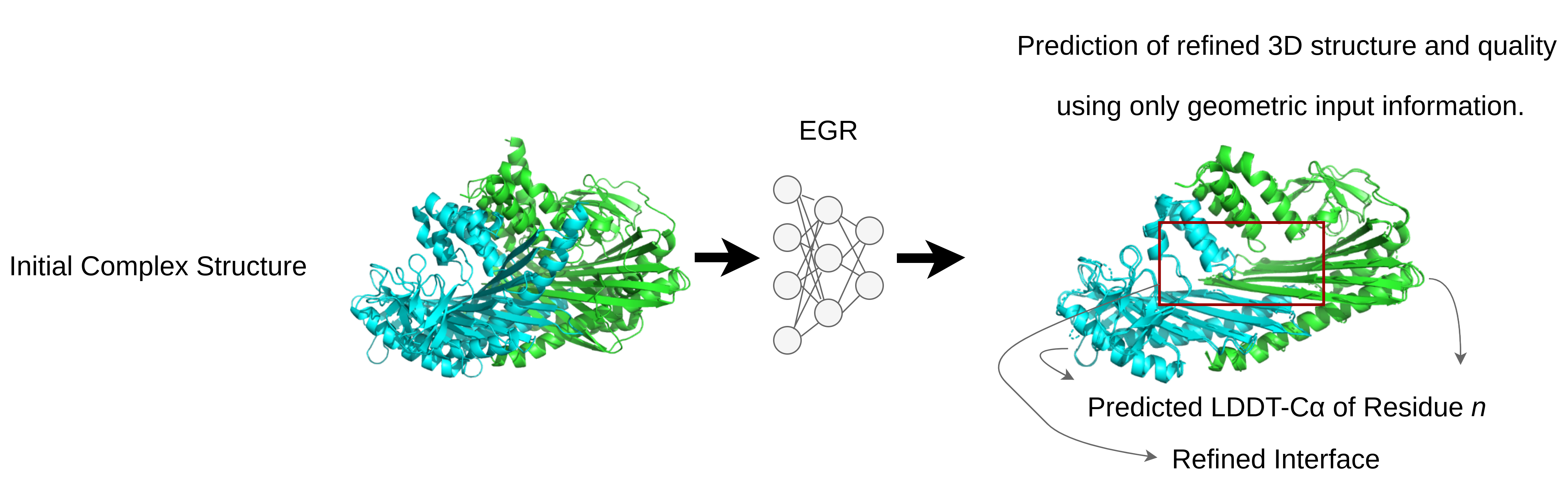
Figure 1: An overview of the structure refinement and assessment problem addressed by EGR.

Here, we introduce EGR, a novel E(3)-equivariant graph deep learning model for multi-task structure refinement and quality assessment of protein complexes - Figure 1. Notably, we exploit equivariant graph neural networks (EGNNs) [12] and careful input regularization to make a direct prediction of the refined structure for an initial protein complex as well as the per-residue quality of the refined structure. Given that our method requires only a single forward pass to finalize its predictions, we achieve significant speed-ups in inference time compared to traditional refinement software solutions. Moreover, our model refines the positions of all atoms in an input protein, making it the first of its kind in DL-based complex structure refinement.

2 Related Work

We now proceed to describe prior works relevant to DL-based structure refinement and assessment.

Biomolecular structure prediction. Until very recently, the conventional means of determining a molecule’s 3D structure would involve costly and time-consuming physical trials performed by experimental scientists [13]. However, using fast computational inference, new DL methods have now made it possible to determine the structures of proteins and other biomolecules in a matter of minutes rather than weeks or months [14, 15]. Such methods have promoted the widespread adoption of structure prediction software [16, 17] and have inspired several new works in DL-driven structure prediction [18, 19].

Protein representation learning (for DL-based molecular modeling). Proteins can be represented in many different forms. For example, representing proteins by their amino acid sequences has been shown to provide powerful structural information by comparing sequences to each other [14] and extracting rich unsupervised learning representations using self-attention Transformers [20]. From a geometric viewpoint, several works have aimed to encode protein structural priors directly within neural network architectures to model proteins hierarchically [21, 22], as computationally-efficient point clouds [23, 24], or as k-nearest neighbors (k-NN) geometric graphs [25, 26] for tasks such as protein function prediction [27], protein model quality assessment [28], and protein interaction region prediction [29].

Applications of structure prediction methods. Markedly, structure prediction models have been applied to predict the structures of all proteins in the human proteome and have aided in efforts to better understand the mechanisms underlying disordered proteins [30]. Moreover, DL-based structure prediction methods have accelerated the discovery of promising drug candidates for therapeutics research [31] and have enabled fast virtual drug screening [32] and materials discovery [33] at scale.

Deep learning for protein-protein docking. Recent advancements in geometric deep learning have supported the development of new DL-based models for rigid body protein-protein docking [34], as well as docking in a single-shot setting [35]. In addition, previous DL models for single-chain protein structure prediction have been repurposed to predict protein complex structures [36] and refine the geometry of side-chain atoms [37].

Deep learning for protein structure refinement. DL models have also been used to guide the refinement of residue positions within tertiary protein structures [38] or predict refined residue positions using indirect target values such as inter-residue distances [39, 40]. Unfortunately, such methods, following refinement, require all-atom restoration procedures as a post-processing step to recover the positions of backbone and side-chain atoms. Promisingly, [41] have begun exploring the use of DL models for all-atom refinement of protein tertiary structures, however, this method has demonstrated success solely for tertiary structures due to its high computational memory complexity.

Deep learning for protein structure quality assessment. As DL-driven structure prediction methods have matured, new methods for quality assessment (QA) of protein structures have also been developed to facilitate automatic ranking of protein structures. In particular, 2D convolutional neural networks (CNNs) [42], 3D CNNs [43], and GNNs [44, 45, 9] have recently been adopted for structure ranking.

Incorporating symmetries in GNNs. Embuing neural networks with inductive priors has a longstanding history in the field [46, 47, 48]. Priors of particular importance for 3D structure modeling include rotation [49] and translation [50] equivariance. Such priors form the basis of 3D Euclidean transformations that can now directly be found within neural network layers [51, 52, 12, 53, 54] to increase networks’ data efficiency and generalization capabilities [55, 56]. Our work follows that of [12] to incorporate E(3)-equivariance in our message passing neural network for 3D structure refinement and quality assessment. However, we go beyond this method by adding skip connections shown to improve gradient flow after position updates, regularizing node input features according to geometric priors for 3D molecules, and employing loss functions for refinement and quality assessment in a semi-supervised manner, respectively.

Contributions.
Our work builds upon prior works by making the following contributions:

• We provide the first example of applying deep learning to the task of all-atom refinement of protein complex structures.

• We provide the first example of applying equivariant graph message passing to the multi-task setting of refining and assessing protein complex structures concurrently.

• We introduce the new semi-supervised EGR model, showcasing its effective use in improving the structure of interface regions between protein chains and estimating its confidence in such improvements.

3 EGR Model

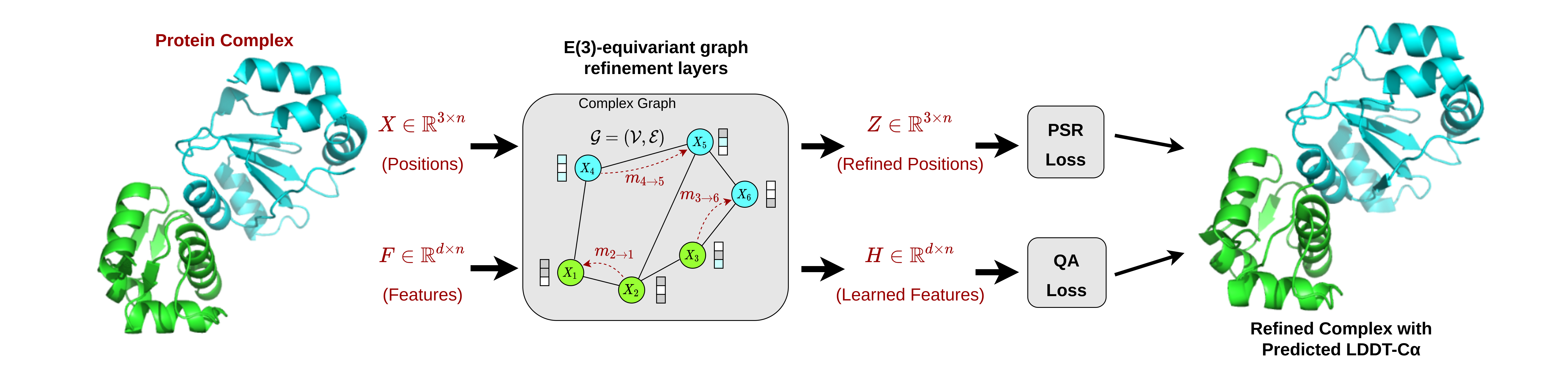
Figure 2: EGR model architecture.

We now turn to describe the EGR model, which is shown in Figure 1 and detailed in Figure 2. The EGR model receives as its input a single 3D protein complex graph representing an initial decoy structure for a given protein target. As such, all chains in the complex are modeled within the same homogeneous input graph structure. As described in Appendix B, we differentiate pairs of atoms belonging to different chains using a one-hot encoded edge feature to initialize the EGR model with knowledge of the complex’s separate chains. In doing so, we allow for structural flexibility of each protein chain in our work, without assuming any rigid conformations within a complex. Notably, our model does this while being trained using only geometric information obtained from each input protein, as it does not make use of any coevolutionary or hand-crafted features for the task at hand.

K-NN graph representation. The input protein complex graphs for our model are constructed using a spatial k-NN algorithm, where a graph $\mathcal{G=(V,E)}$ treats the protein’s atoms as its nodes and denotes each atom’s initial features as $\mathbf{F}\in\mathbb{R}^{d\times n}$ (e.g., atom type) and its positions in $\mathbb{R}^{3}$ as $\mathbf{X}\in\mathbb{R}^{3\times n}$. The nodes in $\mathcal{G}$ are connected to their 20 closest node neighbors in $\mathbb{R}^{3}$, yielding a total of $n\times 20$ edges within $\mathcal{G}$. In Appendix B, we describe the node features $\mathbf{F}$ in further detail.

E(3)-equivariant transformations. In this work, we argue that E(3)-equivariance offers a suitable inductive prior for modeling 3D protein structures. We make this point based primarily on the computational efficiency of E(3)-equivariant networks today. As such, for data efficiency and generalization capabilities, we then turn to designing a neural network capable of capturing within its hidden layers E(3)-transformations of any input protein, especially since for this task we are left to train on a relatively small number of input examples. Towards this end, we propose the Equivariant Graph Refiner (EGR) model, which combines insights from Equivariant Graph Neural Networks [12], EquiDock [35], and EquiBind [19]. The EGR model learns to transform node features and node positions in $\mathbb{R}^{3}$ to perform graph message passing across each input complex graph. Implicitly, this means our model is exchanging information between protein chains in a complex. More formally, EGR($\mathbf{X}$, $\mathbf{F}$) = $\mathbf{Z}\in\mathbb{R}^{3\times n},\mathbf{H}\in\mathbb{R}^{d\times n}$, where $\mathbf{H}$ represents node embeddings and $\mathbf{Z}$ represents transformed node coordinates. We note that, in practical terms, EGR layers can be stacked sequentially in an E(3)-equivariant manner, such that 3D translations or rotations of an input graph will be reflected in the output of any EGR layer. Namely, for an arbitrary translation vector $\mathbf{b}\in\mathbb{R}^{3}$ and orthogonal matrix $\mathbf{U}\in\mathbf{SO}(3)$, EGR($\mathbf{UX}+\mathbf{b},\mathbf{F}$) = $\textbf{UZ}+\textbf{b},\mathbf{H}$. Subsequently, our definition of a single EGR layer is:

$$\mathbf{m}_{j\rightarrow i}=\varphi^{e}(\mathbf{h}_{i}^{(l)},\mathbf{h}_{j}^{(l)},\mathbf{f}_{j\rightarrow i},\|\mathbf{x}_{i}^{(l)}-\mathbf{x}_{j}^{(l)}\|^{2}),\forall(i,j)\in\mathcal{E}$$ (1)

$$\mathbf{x}_{i}^{(l+1)}=\alpha\mathbf{x}_{i}^{(0)}+(1-\alpha)\mathbf{x}_{i}^{(l)}+\frac{1}{|\mathcal{N}(i)|}\sum_{j\in\mathcal{N}(i)}\frac{(\mathbf{x}_{i}^{(l)}-\mathbf{x}_{j}^{(l)})}{\|\mathbf{x}_{i}^{(l)}-\mathbf{x}_{j}^{(l)}\|+\mathcal{C}}\ \varphi^{x}(\mathbf{m}_{j\rightarrow i})$$ (2)

$$\mathbf{m}_{i}=\frac{1}{|\mathcal{N}(i)|}\sum_{j\in\mathcal{N}(i)}\mathbf{m}_{j\rightarrow i},\forall i\in\mathcal{V}$$ (3)

$$\mathbf{h}_{i}^{(l+1)}=\beta\cdot\varphi^{h}(\mathbf{h}_{i}^{(l)},\mathbf{m}_{i},\mathbf{a}_{i},\mathbf{f}_{i})+(1-\beta)\cdot\mathbf{h}_{i}^{(l)},\forall i\in\mathcal{V},$$ (4)

where $\alpha$ and $\beta$, respectively, represent scalar coordinates-wise and node representations-wise skip connection strengths; $\mathcal{N}(i)$ denotes the graph neighbors of node $i$; $\mathbf{a}_{i}$ are optional SE(3)-invariant attention coefficients [35] derived from $\mathbf{H}$; $\mathcal{C}$ is a normalization constant that we set to $\mathcal{C}=1$; and the remaining $\varphi$ functions are represented as shallow neural networks, with $\varphi^{x}$ producing a single scalar and all others a $d$-dimensional vector. Our rationale for normalizing relative positional displacements (i.e., $\mathbf{x}_{i}^{(l)}-\mathbf{x}_{j}^{(l)}$) by their norm, in a similar manner as [57], is to keep the updated coordinates of each EGR layer from exploding in value when aggregating updates from each successive layer. The term $\mathcal{C}$ is also included here to ensure that Equation 2 is still differentiable and to stabilize the EGR model’s training when using $\mathcal{C}=1$. We note that in our studies here, we compute $a_{i}$ from $\mathbf{H}$ using a variant of the Linear Attention Transformer architecture [58, 59, 60], as described in Appendix B.

3.1 Refining initial coordinates

As mentioned previously, each EGR layer predicts transformed coordinates $\mathbf{Z}$. The output of our model’s last EGR layer, $\mathbf{Z}^{L}$, then serves as our estimate of the input complex’s refined coordinates, $\mathbf{X}^{\prime}$ (i.e., $\mathbf{X}^{\prime}=\mathbf{Z}^{L}$).

Refinement loss. To guide the EGR model towards a refined molecular conformation, we use the Huber loss [61] between the EGR model’s refined coordinates $\mathbf{X}^{\prime}$ and the ground truth coordinates $\mathbf{X}^{*}$. Formally, the EGR model’s loss for refinement (i.e., PSR loss) is:

$$\mathcal{L}_{PSR}^{i}=\begin{cases}\frac{1}{2}(x_{i}^{\prime}-x_{i}^{*})^{2},&\text{if }|x_{i}^{\prime}-x_{i}^{*}|<\delta,\\ \delta*(|x_{i}^{\prime}-x_{i}^{*}|-\frac{1}{2}*\delta)&\text{otherwise}\end{cases}$$

$$\mathcal{L}_{PSR}=\frac{1}{|\mathbf{P}|}\sum_{i\in\mathbf{P}}\mathcal{L}_{PSR}^{i},$$ (5)

where $\mathbf{x}_{i}^{\prime}$ are the model’s predicted coordinates for node $i$, $\mathbf{x}_{i}^{*}$ are the ground truth coordinates for node $i$, and $\mathbf{P}$ is the set of indices of atoms for which ground truth coordinates exist in the corresponding native structure. Additionally, we let $\delta=1.0$ in the context of this study. In the context of refinement, outlier coordinate predictions may occur at any stage during model training, so we must take care to ensure our network’s gradients do not explode or saturate inadvertently. As such, we chose this refinement loss function to make it less sensitive to outliers than a mean squared error (MSE) criterion and for it to be smoother near zero compared to a mean absolute error criterion.

Positional reconstruction. Immediately before training, we inject random Gaussian noise into the initial state of our node positions. This corresponds to a small corruption of the location of each atom in an input protein. This methodology follows closely after the Noisy Nodes methodology from [62] and, as such, may facilitate better learning over the manifold of ground truth structures. We study the behavior of the EGR model with and without positional corruption in Section A.

3.2 Assessing structure quality

Following refinement of initial node coordinates, the EGR model also predicts new embeddings for each node, $\mathbf{H}$. Intuitively, we consider $\mathbf{H}$ to be the model’s knowledge of its predicted molecular structure as defined by $\mathbf{X}^{\prime}$. As such, using $\mathbf{H}$, we train an additional head of the network to predict an estimate of the structural accuracy of $\mathbf{X}^{\prime}$.

Quality assessment loss. We formulate assessment of a predicted structure’s quality as a node regression task. Under this framework, we employ an MSE loss to train the second head of the network to predict the carbon-alpha (C$\alpha$) atom local Distance Difference Test (LDDT-C$\alpha$) value [63] of each residue in the complex graph. Formally, the EGR model’s loss for quality assessment (i.e., QA loss) is:

$$\mathcal{L}_{QA}=\frac{1}{|\mathbf{C}|}\sum_{i\in\mathbf{C}}\|\mathbf{q}_{i}^{\prime}-\mathbf{q}_{i}^{*}\|^{2},$$ (6)

where $\mathbf{q}_{i}^{\prime}$ is the model’s predicted LDDT-C$\alpha$ for node $i$, $\mathbf{q}_{i}^{*}$ is the ground truth LDDT-C$\alpha$ for node $i$, and $\mathbf{C}$ is the set of C$\alpha$ atom indices in the input graph. As demonstrated by [14], models trained to predict such a quantity can produce reasonable accuracy estimates for predicted structures, taking one step towards making the EGR model more interpretable for its users.

3.3 Learning paradigm

As mentioned previously, not all atoms in an input decoy structure have a corresponding position in the ground truth structure. Moreover, since during training we can only calculate the ground truth LDDT labels for the input graph’s C$\alpha$ atoms, the EGR model jointly learns to predict refined structures and LDDT-C$\alpha$ scores in a semi-supervised end-to-end manner.

4 Experiments

4.1 Data

For the task of complex structure refinement and assessment, we introduce new Protein Structure Refinement (PSR) datasets comprised of 46,174 homomeric and heteromeric protein complex structural decoys, corresponding to 3,498 unique protein targets. The proteins comprising these datasets (i.e., PSR-Dockground, PSR-DeepHomo, and PSR-EVCoupling) are originally derived from the Dockground [64], DeepHomo [65], and EVCoupling [66] datasets, respectively. The Dockground dataset provides decoy structures of various structural error ranges for each protein target, so we directly include its 1-6 $\mathrm{\text{\r{A}}}$ decoys and their ground truth structures in our PSR dataset. As the DeepHomo and EVCoupling datasets only provide ground truth structures for each of their protein targets, to generate each target’s decoy structures for refinement, we subsequently use AlphaFold-Multimer [36] to predict and select the best decoy structure for each of these datasets’ protein targets. Using TM-score [67], we then uniquely superimpose all ground truth target structures corresponding to each decoy structure to ensure the coordinate systems of both decoy and target structures are aligned before model training. To support the reproducibility of our work, we make our PSR datasets publicly available along with standardized training, validation, and testing splits of the input proteins.

Motivation for introducing new datasets. To the best of our knowledge, our work is the first to introduce cross-validation datasets curated for structural refinement of protein complexes, datasets that we have intentionally designed to be amenable to machine learning methods. In constructing these datasets, we sought to make use of existing protein data sources to maximize their size and structural scope. Notably, since the average structural quality of AlphaFold-Multimer for DeepHomo and EVCoupling proteins is reasonably high, we included proteins from the Dockground dataset to diversify the overall quality of structures in our PSR dataset.

Overlap Reduction. Our constituent PSR datasets are initially combined using random population-proportionate sampling according to a protein’s type and dataset of origin (i.e., Dockground-Heteromer, DeepHomo-Homomer, and EVCoupling-Heteromer). Using MMseqs2 [68], these proportionate splits are then filtered such that no split contains a protein chain with more than 30% sequence similarity to any chain in another split, across all datasets employed in this study. This filtering technique, among others, was chosen to satisfy multiple practical criteria for tasks in this domain: assurance that models (1) cross-validated on such splits do not overfit w.r.t. homology [69] or structural similarity [70] between proteins and (2) will be trained on a sufficient number of input proteins to enable generalization to unseen data.

Test Datasets. The first test dataset we use to evaluate models performing best on our PSR dataset’s validation split is comprised of complexes originally held out from our PSR dataset. As such, this PSR test dataset is comprised of Dockground, DeepHomo, and EVCoupling proteins that have previously been filtered according to 30% sequence similarity. Following the work of [36], we then adopt the heteromeric Benchmark 2 dataset for blind evaluation of our model’s generalization for the task of refinement. Additionally, to score our model’s ability to estimate the quality of a protein complex, we curated a new M4S dataset for complex quality assessment. This dataset consists of randomly-sampled heteromeric protein complexes available in the Protein Data Bank (PDB), where each of the 11 selected complexes was first subjected to 30% sequence identity filtering w.r.t. all of our other cross-validation dataset splits, yielding 1,160 decoys across 11 targets for QA benchmarking.

4.2 Evaluation Setup

Baselines. Modeller [71] is a classical refinement program for 3D protein structures, with support for modeling protein complexes in particular. We also include a version of EGR trained for only C$\alpha$ atom refinement and assessment (i.e., EGR-C$\alpha$) to evaluate Modeller’s ability to reconstruct all-atom structures from the output C$\alpha$ atom coordinates of EGR-C$\alpha$. GalaxyRefineComplex [72] is another popular refinement protocol, one specifically designed for refining structural interfaces between chains in a protein complex. Similarly, we also include GNNRefine [40], which uses GNN-based distance predictions to drive tertiary structural refinement with PyRosetta [73]. We note that we are only able to include GalaxyRefineComplex and GNNRefine’s results on our smaller Benchmark 2 test dataset, as their extraordinarily high refinement runtimes (e.g., 1,200 seconds per decoy with 16 CPU threads) prevent us from evaluating their performance in a reasonable amount of time on our full PSR test dataset consisting of over 5,000 complexes. For our remaining all-atom baselines, we selected two recent geometric deep learning methods with which to compare the EGR model’s performance for all-atom refinement and QA. These methods include SE(3)-Transformers (SETs) [52] and Steerable Equivariant Graph Neural Networks (SEGNNs) [53], both of which have previously been evaluated for their ability to model 3D molecular systems. We evaluate these models using default hyperparameters specified by the authors of each method. Regarding QA, besides including all geometric deep learning methods trained to predict per-residue LDDT-C$\alpha$ scores as baselines, we also compare EGR-AllAtom and EGR-C$\alpha$ to GNN_DOVE [74], a state-of-the-art (SOTA) graph deep learning method for all-atom protein complex structure QA.

EGR Models. In addition to our original EGR model (i.e., EGR-AllAtom), we include three separate versions of the EGR model where we individually remove node or edge-specific features from our input graphs during training and test time. These versions are the EGR model without positional corruption (i.e., EGR-AllAtom-NPC), the model without atom-wise protein surface proximities (i.e., EGR-AllAtom-NSP), and the model without edge-wise relative geometric features (i.e., EGR-AllAtom-NRGF). Such versions are listed in Appendix A to serve as ablation studies on the EGR model, to understand the relative importance of individual input features in our datasets.

Evaluation Metrics. For the task of refinement, for all relevant metrics we report the change in the metric’s value (i.e., the $\Delta$ metric) when comparing a model’s refined structure and the original decoy structure. To evaluate the structural quality of a protein complex, we use the DockQ score [75], interface root mean squared deviation (iRMSD), ligand RMSD (LRMSD), fraction of decoy DockQ scores improved (FI-DockQ), and average percentage of decoy DockQ score improvement (API-DockQ). Here, iRMSD is the mean squared error (MSE) between the atoms of the predicted and ground truth inter-chain interaction regions, and LRMSD is the MSE between the atoms of the predicted and ground truth ligand chains, respectively. Additionally, $F_{nat}$ is the fraction of native contacts found in a decoy structure. Formally, DockQ score can be calculated using Equations 7 and 8, letting $d_{1}=8.5$ and $d_{2}=1.5$:

$$RMSD_{\text{scaled }}\left(RMSD,d_{i}\right)=\frac{1}{1+\left(\frac{RMSD}{d_{i}}\right)^{2}}$$ (7)

$$\text{DockQ}=\frac{1}{3}\left(F_{\text{nat }}+RMSD_{\text{scaled }}\left(LRMSD,d_{1}\right)+RMSD_{\text{scaled }}\left(iRMSD,d_{2}\right)\right).$$ (8)

To evaluate a model’s ranking ability, we use two common metrics, its Top-$N$ hit rate and ranking loss [76, 5]. A model’s hit rate is defined as the fraction of protein target complexes where the model ranked at least one acceptable or higher quality decoy within its predicted list of Top-$N$ decoys. A hit rate is represented by three numbers separated by the character /. The three numbers, in order, represent how many decoys with acceptable or higher quality, medium or higher quality, and high quality were among the Top-$N$ ranked decoys. In this work, we employ the Top-10 hit rate measure. Similarly, a per-target ranking loss is defined as the difference between the DockQ score of a target’s native structure and the decoy for which the model predicted the highest structural quality. As such, a low ranking loss reflects a model’s ability to successfully rank decoys for downstream tasks.

Implementation Details. We train all our models using the AdamW optimizer [77] and perform early stopping with a patience of 50 epochs based on the average full-complex RMSD of a model’s predictions on our PSR dataset’s validation split. All hyperparameters and protein graph features employed are described in Appendix B. Source code to perform fast structural refinement and quality assessment using our provided model weights can be found at https://github.com/BioinfoMachineLearning/DeepRefine.

4.3 Results

Table 1: Performance of different refinement methods on each test dataset.

$\Delta$Metric	DockQ $\uparrow$	iRMSD $\downarrow$	LRMSD $\downarrow$	FI-DockQ $\uparrow$	API-DockQ $\uparrow$
			PSR-Dockground (4,799)
Modeller	+0.0002	-0.6331	-1.0027	63.03%	0.32%
EGR-C$\alpha$-Modeller	+0.0053 $\pm$ 0.0011	-1.2285 $\pm$ 0.0330	-3.5226 $\pm$ 0.3125	79.30% $\pm$ 0.93%	0.89% $\pm$ 0.15%
SET-AllAtom	+0.0132 $\pm$ 0.0040	-0.8808 $\pm$ 0.1158	-1.6478 $\pm$ 0.1047	84.90% $\pm$ 1.13%	1.69% $\pm$ 0.35%
SEGNN-AllAtom	+0.0144 $\pm$ 0.0024	-2.4562 $\pm$ 0.0499	-6.6603 $\pm$ 0.6702	94.46% $\pm$ 0.60%	1.89% $\pm$ 0.29%
EGR-AllAtom	+0.0097 $\pm$ 0.0002	-0.6274 $\pm$ 0.0669	-2.5561 $\pm$ 0.1584	83.66% $\pm$ 0.49%	1.59% $\pm$ 0.11%
			PSR-DeepHomo (376)
Modeller	-0.2465	+1.5912	+5.3457	8.24%	0.53%
EGR-C$\alpha$-Modeller	-0.2796 $\pm$ 0.0055	+2.2075 $\pm$ 0.0839	+6.1711 $\pm$ 0.1842	8.16% $\pm$ 0.76%	1.17% $\pm$ 0.18%
SET-AllAtom	-0.0034 $\pm$ 0.0003	+0.0275 $\pm$ 0.0050	+0.0273 $\pm$ 0.0104	27.39% $\pm$ 4.36%	0.20% $\pm$ 0.08%
SEGNN-AllAtom	-0.0468 $\pm$ 0.0091	+0.2950 $\pm$ 0.0741	+0.3593 $\pm$ 0.1722	16.31% $\pm$ 3.54%	0.87% $\pm$ 0.20%
EGR-AllAtom	-0.0006 $\pm$ 0.0018	+0.0121 $\pm$ 0.0054	+0.0013 $\pm$ 0.0028	45.12% $\pm$ 6.99%	0.41% $\pm$ 0.03%
			PSR-EVCoupling (195)
Modeller	-0.1738	+1.1467	+4.9877	7.18%	0.74%
EGR-C$\alpha$-Modeller	-0.2150 $\pm$ 0.0073	+1.9651 $\pm$ 0.0647	+5.8477 $\pm$ 0.7759	9.91% $\pm$ 1.74%	1.49% $\pm$ 0.37%
SET-AllAtom	-0.0016 $\pm$ 0.0002	+0.0149 $\pm$ 0.0007	+0.0108 $\pm$ 0.0040	27.86% $\pm$ 5.24%	0.31% $\pm$ 0.11%
SEGNN-AllAtom	-0.0250 $\pm$ 0.0069	+0.1646 $\pm$ 0.0633	+0.2400 $\pm$ 0.1044	18.29% $\pm$ 3.41%	0.89% $\pm$ 0.18%
EGR-AllAtom	+0.0010 $\pm$ 0.0010	+0.0026 $\pm$ 0.0031	-0.0059 $\pm$ 0.0017	43.93% $\pm$ 5.00%	0.48% $\pm$ 0.03%
			Benchmark 2 (17)
Modeller	-0.1855	+0.7939	+3.0277	5.88%	0.60%
GalaxyRefineComplex	-0.0074	+0.0778	-0.0246	22.22%	2.12%
GNNRefine	+0.0025	+0.0226	+0.0602	47.06%	1.26%
EGR-C$\alpha$-Modeller	-0.2644 $\pm$ 0.0437	+2.118 $\pm$ 0.7832	+5.9196 $\pm$ 1.8589	15.69% $\pm$ 2.77%	1.28% $\pm$ 0.84%
SET-AllAtom	-0.0078 $\pm$ 0.0015	+0.0729 $\pm$ 0.0186	+0.0469 $\pm$ 0.0114	29.63% $\pm$ 2.62%	0.33% $\pm$ 0.14%
SEGNN-AllAtom	-0.0328 $\pm$ 0.0062	+0.0807 $\pm$ 0.0790	+0.0781 $\pm$ 0.1371	31.37% $\pm$ 5.54%	1.24% $\pm$ 0.59%
EGR-AllAtom	-0.0010 $\pm$ 0.0028	-0.0002 $\pm$ 0.003	-0.0121 $\pm$ 0.0021	43.14% $\pm$ 10.00%	0.59% $\pm$ 0.08%

Blind Refinement. In Table 1, we see that the all-atom EGR model surpasses the refinement performance of all other baseline methods except on the low initial quality structures from Dockground. We observe that methods outperforming EGR on the Dockground targets also appear to underperform EGR on targets from datasets of higher initial structural quality, suggesting these methods are overfitting to low-quality structures in the PSR training dataset. EGR-AllAtom, however, appears to generalize better to all test datasets compared to any other method (accounting for the fact that GNNRefine may have seen overly-similar proteins during training), with a computational complexity (e.g., average of 5 seconds) orders of magnitude lower than that of methods such as GalaxyRefineComplex and GNNRefine (e.g., average of 1,200 and 600 seconds, respectively).

Table 2: Hit rate performance of different QA methods on the M4S test dataset.

ID	EGR-C$\alpha$-Modeller	SET-AllAtom	SEGNN-AllAtom	EGR-AllAtom	GNN_DOVE	Top-10 Best
7AOH	10/10/6	9/8/6	9/9/9	9/9/9	9/9/0	10/10/10
7D7F	0/0/0	2/0/0	0/0/0	0/0/0	0/0/0	5/0/0
7AMV	10/10/8	10/10/5	10/10/9	10/10/5	10/10/6	10/10/10
7OEL	10/10/0	10/10/0	10/9/0	10/9/0	10/10/0	10/10/0
7O28	10/10/0	10/10/0	10/10/0	10/10/0	10/10/0	10/10/0
7MRW	6/5/0	0/0/0	0/0/0	0/0/0	0/0/0	10/10/0
7D3Y	0/0/0	0/0/0	0/0/0	1/0/0	0/0/0	10/0/0
7NKZ	10/10/9	10/9/9	10/10/3	10/9/9	10/9/9	10/10/10
7LXT	10/10/0	4/3/0	6/5/0	8/7/0	1/0/0	10/10/0
7KBR	10/10/10	10/10/10	10/10/10	10/10/9	10/10/9	10/10/10
7O27	10/5/0	10/7/0	10/6/0	10/4/0	10/4/0	10/10/0
Summary	9/9/4	9/8/4	8/8/4	9/8/4	8/7/3	11/9/4

Table 3: Ranking loss of different QA methods on the M4S test dataset.

ID	EGR-C$\alpha$-Modeller	SET-AllAtom	SEGNN-AllAtom	EGR-AllAtom	GNN_DOVE
7AOH	0.0610	0.9280	0.9280	0.0350	0.9280
7D7F	0.4700	0.4700	0.4710	0.4590	0.0030
7AMV	0.1730	0.3420	0.0130	0.3420	0.3420
7OEL	0.2100	0.2100	0.3790	0.2100	0.2100
7O28	0.2330	0.0240	0.2740	0.2440	0.2440
7MRW	0.6000	0.5550	0.6030	0.5550	0.5980
7D3Y	0.3240	0.2950	0.1740	0.2950	0.2950
7NKZ	0.0220	0.1100	0.1830	0.4590	0.4590
7LXT	0.0500	0.2950	0.2950	0.3890	0.2950
7KBR	0.1700	0.1520	0.0520	0.1520	0.0680
7O27	0.3340	0.3340	0.3650	0.3180	0.3340
Summary	0.2406 $\pm$ 0.1801	0.3377 $\pm$ 0.2486	0.3397 $\pm$ 0.2613	0.3144 $\pm$ 0.1506	0.3432 $\pm$ 0.2538

Blind Quality Assessment. Table 2 summarizes a few key findings regarding models’ QA performance. The first is that both EGR-AllAtom and EGR-C$\alpha$-Modeller outperform GNN_DOVE, the state-of-the-art QA predictor for protein complexes, on a large collection of decoy structures. Interestingly, we also find that modeling protein complexes at the granularity of C$\alpha$ atoms leads to EGR-C$\alpha$-Modeller achieving new SOTA results. This suggests interesting avenues for future research into molecular modeling for structural QA. Nonetheless, within a single model, EGR-AllAtom can outperform all other methods for QA while simultaneously achieving SOTA performance for refinement, demonstrating the complementarity of the two tasks in the context of all-atom modeling.

Original Decoy

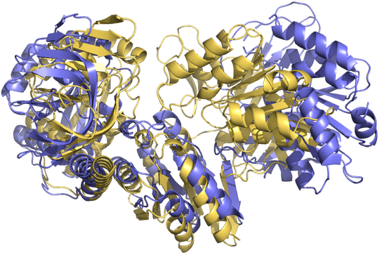
RMSD = 8.715

Modeller-Refined Decoy

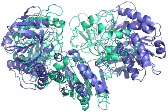
RMSD = 10.131

EGR-Refined Decoy

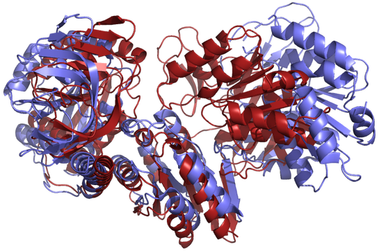
RMSD = 8.636

Figure 3: A cherry-picked example of a test protein complex (PDB ID: 6GS2) successfully refined by EGR. Note in all the above subfigures the ground truth structure is highlighted in the color slate.

Visualizations. We display in Figure 3 a successful example of a PSR test protein other refinement methods (e.g., Modeller) cannot refine but that EGR nonetheless can refine atomistically.

Limitations. Although EGR has driven significant progress in protein complex structure refinement and assessment, the model is currently only able to improve the structure of inter-chain interfaces marginally on average due partly to its relatively small training dataset size and partly to limited computing resources available for generating sufficiently large datasets. As such, we conjecture that new large datasets comprised of medium and high-quality complex decoys are required for refinement methods to better generalize their predictions to higher-quality structures. We leave an exploration of such ideas for future work.

5 Conclusion

We presented EGR which introduces an E(3)-equivariant method for refining and assessing the quality of 3D protein complex structures. Our experiments validate the effectiveness of EGR for structural refinement and assessment using a diverse, open-source collection of protein complexes and establish a baseline for future studies in geometric deep learning for protein structure refinement and analysis. Used with care and with feedback from domain experts, we believe EGR could encourage the use of DL models in responsible drug discovery and development.

6 Acknowledgments

The project is partially supported by two NSF grants (DBI 1759934 and IIS 1763246), one NIH grant (GM093123), three DOE grants (DE-SC0020400, DE-AR0001213, and DE-SC0021303), and the computing allocation on the Summit compute cluster provided by Oak Ridge Leadership Computing Facility (Contract No. DE-AC05-00OR22725).

Appendix A Additional Results

Table 4: Ablation studies on the EGR model using each test dataset.

$\Delta$Metric	DockQ $\uparrow$	iRMSD $\downarrow$	LRMSD $\downarrow$	FI-DockQ $\uparrow$	API-DockQ $\uparrow$
			PSR-Dockground (4,799)
EGR-AllAtom-NPC	+0.0083 $\pm$ 0.0006	-0.6549 $\pm$ 0.1589	-2.5129 $\pm$ 0.1584	82.95% $\pm$ 1.98%	1.46% $\pm$ 0.09%
EGR-AllAtom-NSP	+0.0048 $\pm$ 0.0039	-0.4881 $\pm$ 0.1622	-1.5799 $\pm$ 0.5891	74.15% $\pm$ 1.77%	1.46% $\pm$ 0.09%
EGR-AllAtom-NRGF	+0.0035 $\pm$ 0.0018	-0.4817 $\pm$ 0.0470	-0.8711 $\pm$ 0.2320	73.61% $\pm$ 2.39%	0.71% $\pm$ 0.19%
EGR-AllAtom	+0.0097 $\pm$ 0.0002	-0.6274 $\pm$ 0.0669	-2.5561 $\pm$ 0.2893	83.66% $\pm$ 0.49%	1.59% $\pm$ 0.11%
			PSR-DeepHomo (376)
EGR-AllAtom-NPC	-0.0011 $\pm$ 0.0019	+0.0044 $\pm$ 0.0021	-0.0003 $\pm$ 0.0010	36.08% $\pm$ 9.57%	0.30% $\pm$ 0.08%
EGR-AllAtom-NSP	0.0000 $\pm$ 0.0015	+0.0088 $\pm$ 0.0041	+0.0008 $\pm$ 0.0015	46.10% $\pm$ 11.47%	0.39% $\pm$ 0.10%
EGR-AllAtom-NRGF	-0.1296 $\pm$ 0.0276	+0.7784 $\pm$ 0.1660	+0.5925 $\pm$ 0.1625	10.28% $\pm$ 3.83%	1.11% $\pm$ 0.16%
EGR-AllAtom	-0.0006 $\pm$ 0.0018	+0.0121 $\pm$ 0.0054	+0.0013 $\pm$ 0.0028	45.12% $\pm$ 6.99%	0.41% $\pm$ 0.03%
			PSR-EVCoupling (195)
EGR-AllAtom-NPC	-0.0003 $\pm$ 0.0014	+0.0007 $\pm$ 0.0009	-0.0041 $\pm$ 0.0012	33.16% $\pm$ 10.60%	0.31% $\pm$ 0.08%
EGR-AllAtom-NSP	+0.0007 $\pm$ 0.0013	+0.0021 $\pm$ 0.0016	-0.0057 $\pm$ 0.0020	39.66% $\pm$ 9.02%	0.39% $\pm$ 0.13%
EGR-AllAtom-NRGF	-0.0743 $\pm$ 0.0183	+0.4843 $\pm$ 0.1084	+0.3218 $\pm$ 0.1003	11.11% $\pm$ 4.48%	1.07% $\pm$ 0.18%
EGR-AllAtom	+0.0010 $\pm$ 0.0010	+0.0026 $\pm$ 0.0031	-0.0059 $\pm$ 0.0017	43.93% $\pm$ 5.00%	0.48% $\pm$ 0.03%
			Benchmark 2 (17)
EGR-AllAtom-NPC	-0.0006 $\pm$ 0.0014	-0.0038 $\pm$ 0.0008	-0.0127 $\pm$ 0.0067	41.18% $\pm$ 12.71%	0.26% $\pm$ 0.20%
EGR-AllAtom-NSP	-0.0007 $\pm$ 0.0030	-0.0049 $\pm$ 0.0016	-0.0185 $\pm$ 0.0020	41.18% $\pm$ 12.71%	0.51% $\pm$ 0.18%
EGR-AllAtom-NRGF	-0.0070 $\pm$ 0.0054	+0.0010 $\pm$ 0.0027	-0.0126 $\pm$ 0.0004	27.45% $\pm$ 7.34%	0.22% $\pm$ 0.14%
EGR-AllAtom	-0.0010 $\pm$ 0.0028	-0.0002 $\pm$ 0.003	-0.0121 $\pm$ 0.0021	43.14% $\pm$ 10.00%	0.59% $\pm$ 0.08%

Table 5: Performance of different refinement methods, including ablation studies, on all test datasets.

$\Delta$Metric	Fraction of Native Contacts $\uparrow$	Fraction of Non-Native Contacts $\downarrow$
		PSR-Dockground (4,799)
Modeller	+0.0003	+0.0009
EGR-C$\alpha$-Modeller	+0.0112 $\pm$ 0.0034	+0.0029 $\pm$ 0.0007
SET-AllAtom	+0.0392 $\pm$ 0.0126	+0.0109 $\pm$ 0.0008
SEGNN-AllAtom	+0.0322 $\pm$ 0.0072	+0.0094 $\pm$ 0.0006
EGR-AllAtom-NPC	+0.0284 $\pm$ 0.0024	+0.0116 $\pm$ 0.0001
EGR-AllAtom-NSP	+0.0153 $\pm$ 0.0110	+0.0085 $\pm$ 0.0026
EGR-AllAtom-NRGF	+0.0128 $\pm$ 0.0110	+0.0098 $\pm$ 0.0018
EGR-AllAtom	+0.0324 $\pm$ 0.0027	+0.0122 $\pm$ 0.0011
		PSR-DeepHomo (376)
Modeller	-0.1844	+0.2445
EGR-C$\alpha$-Modeller	-0.1630 $\pm$ 0.0106	+0.3441 $\pm$ 0.0072
SET-AllAtom	+0.0014 $\pm$ 0.0013	+0.0144 $\pm$ 0.0043
SEGNN-AllAtom	-0.0152 $\pm$ 0.0064	+0.1032 $\pm$ 0.0349
EGR-AllAtom-NPC	-0.0009 $\pm$ 0.0063	+0.0029 $\pm$ 0.0069
EGR-AllAtom-NSP	+0.0049 $\pm$ 0.0065	+0.0143 $\pm$ 0.0126
EGR-AllAtom-NRGF	-0.0942 $\pm$ 0.0672	+0.2930 $\pm$ 0.0665
EGR-AllAtom	+0.0046 $\pm$ 0.0029	+0.0157 $\pm$ 0.0016
		PSR-EVCoupling (195)
Modeller	-0.1334	+0.1971
EGR-C$\alpha$-Modeller	-0.1343 $\pm$ 0.0131	+0.3100 $\pm$ 0.0082
SET-AllAtom	+0.0020 $\pm$ 0.0014	+0.0110 $\pm$ 0.0064
SEGNN-AllAtom	-0.0005 $\pm$ 0.0030	+0.0873 $\pm$ 0.0315
EGR-AllAtom-NPC	0.0003 $\pm$ 0.0045	+0.0009 $\pm$ 0.0049
EGR-AllAtom-NSP	+0.0047 $\pm$ 0.0049	+0.0105 $\pm$ 0.0086
EGR-AllAtom-NRGF	-0.0482 $\pm$ 0.0475	+0.2064 $\pm$ 0.0555
EGR-AllAtom	+0.0065 $\pm$ 0.0015	+0.0113 $\pm$ 0.0022
		Benchmark 2 (17)
Modeller	-0.1645	+0.2232
GalaxyRefineComplex	-0.0001	+0.0601
GNNRefine	+0.0087	+0.0707
EGR-C$\alpha$-Modeller	-0.1794 $\pm$ 0.0405	+0.3915 $\pm$ 0.0432
SET-AllAtom	+0.0072 $\pm$ 0.0033	+0.0212 $\pm$ 0.0034
SEGNN-AllAtom	-0.0275 $\pm$ 0.0080	+0.0781 $\pm$ 0.0058
EGR-AllAtom-NPC	-0.0004 $\pm$ 0.0067	0.0000 $\pm$ 0.0057
EGR-AllAtom-NSP	+0.0005 $\pm$ 0.0088	+0.0053 $\pm$ 0.0086
EGR-AllAtom-NRGF	-0.0157 $\pm$ 0.0142	-0.0075 $\pm$ 0.0099
EGR-AllAtom	+0.0014 $\pm$ 0.006	+0.0110 $\pm$ 0.0037

In Table 4, we investigate the effect of removing individual components or input features from the EGR model. We then compare these results to the baseline EGR model to assess these components’ relative importance on generalization and model accuracy. Similarly, in addition to iRMSD, LRMSD, FI-DockQ, and API-DockQ, we can also inspect the fraction of native and non-native inter-chain contacts present in a structural decoy for a protein target. Such measures can yield insights into how the interface between two or more chains in a complex was formed and whether or not the interface is near-native. We show the results of these measures in Table 5.

Appendix B Implementation Details

Expanded discussion of attention mechanism. As mentioned in Section 3, within each EGR layer, we compute $a_{i}$ from $\mathbf{H}$ using a variant of the Linear Attention Transformer architecture [58, 59, 60]. In particular, we compute not only global attention scores for each atom pair, but we also calculate local, atom-wise attention scores using windows of size $128\times 128$. To perform global attention, the most computationally-expensive of these operations, in linear time, a key insight from [59] is that

$$\mathbf{D}(\mathbf{Q},\mathbf{K},\mathbf{V})=\frac{\mathbf{Q}\mathbf{K}^{\top}}{n}\mathbf{V}=\mathbf{E}(\mathbf{Q},\mathbf{K},\mathbf{V})=\frac{\mathbf{Q}}{\sqrt{n}}\left(\frac{\mathbf{K}^{\top}}{\sqrt{n}}\mathbf{V}\right)$$ (9)

where the commutativity of scalar multiplication with matrix multiplication and the associativity of matrix multiplication give us

$$\mathbf{E}(\mathbf{Q},\mathbf{K},\mathbf{V}) =\frac{\mathbf{Q}}{\sqrt{n}}\left(\frac{\mathbf{K}^{\top}}{\sqrt{n}}\mathbf{V}\right)$$ (10)

$$=\frac{1}{n}\mathbf{Q}\left(\mathbf{K}^{\top}\mathbf{V}\right)$$

$$=\frac{1}{n}\left(\mathbf{Q}\mathbf{K}^{\top}\right)\mathbf{V}$$

$$=\frac{\mathbf{Q}\mathbf{K}^{\top}}{n}\mathbf{V},$$

with $\mathbf{D}$ representing standard attention that is quadratic w.r.t. the input sequence length; $\mathbf{E}$ denoting linear attention that is linear w.r.t. the input sequence length; $\mathbf{Q}$, $\mathbf{K}$, and $\mathbf{V}$, respectively, being query, key, and value linear projections of $\mathbf{H}$; and $n$ representing a normalization constant. As such, our global attention calculations remain computationally feasible for large input protein complexes. Our local attention calculations, then, follow closely after those of [78].

Featurization. In each all-atom protein complex graph, we include as a node feature an atom’s type using a 38-dimensional one-hot encoding vector for each atom. Then, to add a new node feature representing the normalized proximity of an atom to the surface of the protein chain to which it belongs, using MSMS [79] we take the complement of each atom’s chain-wise buriedness to derive atomic surface proximities for surface contact modeling [35]. Notably, for the EGR-C$\alpha$-Modeller model, its input graphs are comprised of C$\alpha$ atoms as nodes rather than all available atoms. In such C$\alpha$ atom graphs, we also include node features describing each residue’s dihedral angles [26]. Lastly, we note that in our experiments with the SEGNN, for this model we included an additional type-1 (i.e., vector-valued) node feature describing the coordinates-wise displacement between a given node’s position and the mean atomic coordinates of the protein complex. All node features we selected for all-atom and C$\alpha$-atom graphs are shown in Tables 6 and 7, respectively.

For our graphs’ edge features, we start by adding a binary feature indicating whether or not a pair of connected atoms belong to the same chain. We then add an edge-wise sinusoidal positional encoding of the difference between the source and destination node’s indices in the input graph [8]. As another edge feature, we include a binary value indicating whether or not a pair of atoms are connected by a covalent bond. Our final type-0 edge feature describes the relative geometric features such as distance, direction, and orientation between the local coordinate systems representing the residues corresponding to an atom pair, following [80, 14]. Lastly, in our SEGNN experiments, we also included an additional type-1 edge feature describing the relative coordinates-wise displacement between a connected pair of atoms. All edge features we selected for all-atom and C$\alpha$-atom graphs are shown in Tables 6 and 7, respectively.

Table 6: Summary of EGR’s node and edge features for all-atom graphs. Here, $N$ and $E$ denote the number of nodes and edges in $\mathcal{G}$, respectively.

	Feature	Type	Shape
Node Features	One-hot encoding of atom type	Categorical	$N\times 38$
	Chain-local surface proximity	Numeric	$N\times 1$
Edge Features	Permutation-invariant chain encoding	Categorical	$E\times 1$
	Sinusoidal edge positional encoding	Numeric	$E\times 1$
	Relative geometric features	Numeric	$E\times 12$
	Covalent bond encoding	Categorical	$E\times 1$
Total	Node features		$N\times 39$
	Edge features		$E\times 15$

Table 7: Summary of EGR’s node and edge features for C$\alpha$-atom graphs. Here, $N$ and $E$ denote the number of nodes and edges in $\mathcal{G}$, respectively.

	Feature	Type	Shape
Node Features	One-hot encoding of residue type	Categorical	$N\times 21$
	Chain-local surface proximity	Numeric	$N\times 1$
	Dihedral angle descriptors	Numeric	$N\times 6$
Edge Features	Permutation-invariant chain encoding	Categorical	$E\times 1$
	Sinusoidal edge positional encoding	Numeric	$E\times 1$
	Relative geometric features	Numeric	$E\times 12$
Total	Node features		$N\times 28$
	Edge features		$E\times 14$

Hardware Used. The Oak Ridge Leadership Facility (OLCF) at the Oak Ridge National Laboratory (ORNL) is an open science computing facility that supports HPC research. The OLCF houses the Summit compute cluster. Summit, launched in 2018, delivers 8 times the computational performance of Titan’s 18,688 nodes, using only 4,608 nodes. Like Titan, Summit has a hybrid architecture, and each node contains multiple IBM POWER9 CPUs and NVIDIA Volta GPUs all connected with NVIDIA’s high-speed NVLink. Each node has over half a terabyte of coherent memory (high bandwidth memory + DDR4) addressable by all CPUs and GPUs plus 800GB of non-volatile RAM that can be used as a burst buffer or as extended memory. To provide a high rate of I/O throughput, the nodes are connected in a non-blocking fat-tree using a dual-rail Mellanox EDR InfiniBand interconnect. We used the Summit compute cluster to train all our models.

Software Used. We used Python 3.8 [81], PyTorch 1.10.0 [82], PyTorch Lightning 1.5.10 [83], PyTorch Geometric 2.0.4 [84], and DGL 0.8 [85] to run our deep learning experiments. PyTorch Lightning was used to facilitate model checkpointing, metrics reporting, and distributed data parallelism across 144 Tesla V100 GPUs. A more in-depth description of the software environment used to run inference with our models can be found at https://github.com/BioinfoMachineLearning/DeepRefine.

Further hyperparameters. We use a learning rate of $10^{-4}$ for all EGR models. The learning rate is kept constant throughout each model’s training. Models with the lowest RMSD on our validation data split are then tested on all our sequence-filtered test splits.

Table 8: Hyperparameter search space for all EGR models through which we searched to obtain strong performance on the PSR validation split. The final parameters for the standard EGR model are in bold.

Hyperparameter	Search Space
PSR Loss Weight	1.0 (Based on Loss on Validation Split)
QA Loss Weight	0.05, 0.005
Number of Layers	4, 7
Hidden Dimension	64, 128
Non-Linearities	LeakyReLU, PReLU, SiLU
Learning Rate	0.0001, 0.001
Weight Decay Rate	$10^{-8}$, $\mathbf{10^{-4}}$
Normalization	LayerNorm, GroupNorm, Identity

References

- [1] Victor Spirin and Leonid A. Mirny “Protein complexes and functional modules in molecular networks” In Proceedings of the National Academy of Sciences 100.21, 2003, pp. 12123–12128 DOI: 10.1073/pnas.2032324100
- [2] RP Bahadur and M Zacharias “The interface of protein-protein complexes: analysis of contacts and prediction of interactions” In Cellular and Molecular Life Sciences 65.7 Springer, 2008, pp. 1059–1072
- [3] Thomas Walzthoeni, Alexander Leitner, Florian Stengel and Ruedi Aebersold “Mass spectrometry supported determination of protein complex structure” Theory and simulation / Macromolecular assemblies In Current Opinion in Structural Biology 23.2, 2013, pp. 252–260 DOI: https://doi.org/10.1016/j.sbi.2013.02.008
- [4] Sumudu P Leelananda and Steffen Lindert “Computational methods in drug discovery” In Beilstein journal of organic chemistry 12.1 Beilstein-Institut, 2016, pp. 2694–2718
- [5] Marc F Lensink et al. “Prediction of protein assemblies, the next frontier: The CASP14-CAPRI experiment” In Proteins: Structure, Function, and Bioinformatics 89.12 Wiley Online Library, 2021, pp. 1800–1823
- [6] Mu Gao et al. “High-Performance Deep Learning Toolbox for Genome-Scale Prediction of Protein Structure and Function” In 2021 IEEE/ACM Workshop on Machine Learning in High Performance Computing Environments (MLHPC), 2021, pp. 46–57 IEEE
- [7] Alex Morehead, Chen Chen, Ada Sedova and Jianlin Cheng “DIPS-Plus: The Enhanced Database of Interacting Protein Structures for Interface Prediction” In arXiv preprint arXiv:2106.04362, 2021
- [8] Alex Morehead, Chen Chen and Jianlin Cheng “Geometric Transformers for Protein Interface Contact Prediction” In arXiv preprint arXiv:2110.02423, 2021
- [9] Chen Chen et al. “3D-equivariant graph neural networks for protein model quality assessment” In bioRxiv Cold Spring Harbor Laboratory, 2022
- [10] Kathryn Tunyasuvunakool “The prospects and opportunities of protein structure prediction with AI” In Nature Reviews Molecular Cell Biology Nature Publishing Group, 2022, pp. 1–2
- [11] Jacob Verburgt and Daisuke Kihara “Benchmarking of structure refinement methods for protein complex models” In Proteins: Structure, Function, and Bioinformatics 90.1 Wiley Online Library, 2022, pp. 83–95
- [12] Vıctor Garcia Satorras, Emiel Hoogeboom and Max Welling “E (n) equivariant graph neural networks” In International Conference on Machine Learning, 2021, pp. 9323–9332 PMLR
- [13] Roslyn M Bill et al. “Overcoming barriers to membrane protein structure determination” In Nature biotechnology 29.4 Nature Publishing Group, 2011, pp. 335–340
- [14] John Jumper et al. “Highly accurate protein structure prediction with AlphaFold” In Nature 596.7873 Nature Publishing Group, 2021, pp. 583–589
- [15] Minkyung Baek et al. “Accurate prediction of protein structures and interactions using a three-track neural network” In Science 373.6557 American Association for the Advancement of Science, 2021, pp. 871–876
- [16] Mihaly Varadi et al. “AlphaFold Protein Structure Database: Massively expanding the structural coverage of protein-sequence space with high-accuracy models” In Nucleic acids research 50.D1 Oxford University Press, 2022, pp. D439–D444
- [17] Patrick Cramer “AlphaFold2 and the future of structural biology” In Nature Structural & Molecular Biology 28.9 Nature Publishing Group, 2021, pp. 704–705
- [18] Raphael J.. Townshend et al. “Geometric deep learning of RNA structure” In Science 373.6558, 2021, pp. 1047–1051 DOI: 10.1126/science.abe5650
- [19] Hannes Stärk et al. “Equibind: Geometric deep learning for drug binding structure prediction” In arXiv preprint arXiv:2202.05146, 2022
- [20] Roshan Rao et al. “Transformer protein language models are unsupervised structure learners” In International Conference on Learning Representations, 2021 URL: https://openreview.net/forum?id=fylclEqgvgd
- [21] Vignesh Ram Somnath, Charlotte Bunne and Andreas Krause “Multi-Scale Representation Learning on Proteins” In Advances in Neural Information Processing Systems 34, 2021
- [22] Pedro Hermosilla et al. “Intrinsic-Extrinsic Convolution and Pooling for Learning on 3D Protein Structures” In arXiv preprint arXiv:2007.06252, 2020
- [23] Pablo Gainza et al. “Deciphering interaction fingerprints from protein molecular surfaces using geometric deep learning” In Nature Methods 17.2 Nature Publishing Group, 2020, pp. 184–192
- [24] Freyr Sverrisson, Jean Feydy, Bruno E Correia and Michael M Bronstein “Fast end-to-end learning on protein surfaces” In Proceedings of the IEEE/CVF Conference on Computer Vision and Pattern Recognition, 2021, pp. 15272–15281
- [25] Bowen Jing et al. “Learning from protein structure with geometric vector perceptrons” In arXiv preprint arXiv:2009.01411, 2020
- [26] Wengong Jin, Jeremy Wohlwend, Regina Barzilay and Tommi Jaakkola “Iterative refinement graph neural network for antibody sequence-structure co-design” In arXiv preprint arXiv:2110.04624, 2021
- [27] Vladimir Gligorijević et al. “Structure-based protein function prediction using graph convolutional networks” In Nature communications 12.1 Nature Publishing Group, 2021, pp. 1–14
- [28] Stephan Eismann et al. “Protein model quality assessment using rotation-equivariant, hierarchical neural networks” In arXiv preprint arXiv:2011.13557, 2020
- [29] Bowen Dai and Chris Bailey-Kellogg “Protein interaction interface region prediction by geometric deep learning” In Bioinformatics 37.17 Oxford University Press, 2021, pp. 2580–2588
- [30] Kiersten M Ruff and Rohit V Pappu “AlphaFold and implications for intrinsically disordered proteins” In Journal of Molecular Biology 433.20 Elsevier, 2021, pp. 167208
- [31] Feng Ren et al. “AlphaFold Accelerates Artificial Intelligence Powered Drug Discovery: Efficient Discovery of a Novel Cyclin-dependent Kinase 20 (CDK20) Small Molecule Inhibitor” In arXiv preprint arXiv:2201.09647, 2022
- [32] Pawel Gniewek et al. “Learning physics confers pose-sensitivity in structure-based virtual screening” In arXiv preprint arXiv:2110.15459, 2021
- [33] Artem R Oganov, Chris J Pickard, Qiang Zhu and Richard J Needs “Structure prediction drives materials discovery” In Nature Reviews Materials 4.5 Nature Publishing Group, 2019, pp. 331–348
- [34] Freyr Sverrisson et al. “Physics-informed deep neural network for rigid-body protein docking” In ICLR2022 Machine Learning for Drug Discovery, 2022
- [35] Octavian-Eugen Ganea et al. “Independent SE (3)-Equivariant Models for End-to-End Rigid Protein Docking” In arXiv preprint arXiv:2111.07786, 2021
- [36] Richard Evans et al. “Protein complex prediction with AlphaFold-Multimer” In BioRxiv Cold Spring Harbor Laboratory, 2021
- [37] Akhil Jindal et al. “Side-chain Packing Using SE (3)-Transformer” In PACIFIC SYMPOSIUM ON BIOCOMPUTING 2022, 2021, pp. 46–55 World Scientific
- [38] Naozumi Hiranuma et al. “Improved protein structure refinement guided by deep learning based accuracy estimation” In Nature communications 12.1 Nature Publishing Group, 2021, pp. 1–11
- [39] Md Hossain Shuvo, Muhammad Gulfam and Debswapna Bhattacharya “DeepRefiner: high-accuracy protein structure refinement by deep network calibration” In Nucleic Acids Research 49.W1, 2021, pp. W147–W152 DOI: 10.1093/nar/gkab361
- [40] Xiaoyang Jing and Jinbo Xu “Fast and effective protein model refinement using deep graph neural networks” In Nature Computational Science 1.7 Nature Publishing Group, 2021, pp. 462–469
- [41] Tianqi Wu and Jianlin Cheng “Atomic protein structure refinement using all-atom graph representations and SE(3)-equivariant graph neural networks” In bioRxiv Cold Spring Harbor Laboratory, 2022 DOI: 10.1101/2022.05.06.490934
- [42] Xiao Chen and Jianlin Cheng “DISTEMA: distance map-based estimation of single protein model accuracy with attentive 2D convolutional neural network” In BMC bioinformatics 23.3 Springer, 2022, pp. 1–14
- [43] Guillaume Pagès, Benoit Charmettant and Sergei Grudinin “Protein model quality assessment using 3D oriented convolutional neural networks” In Bioinformatics 35.18 Oxford University Press, 2019, pp. 3313–3319
- [44] Soumya Sanyal et al. “ProteinGCN: Protein model quality assessment using graph convolutional networks” In BioRxiv Cold Spring Harbor Laboratory, 2020
- [45] Federico Baldassarre, David Menéndez Hurtado, Arne Elofsson and Hossein Azizpour “GraphQA: protein model quality assessment using graph convolutional networks” In Bioinformatics 37.3 Oxford University Press, 2021, pp. 360–366
- [46] Peter W Battaglia et al. “Relational inductive biases, deep learning, and graph networks” In arXiv preprint arXiv:1806.01261, 2018
- [47] Reuben Feinman and Brenden M Lake “Learning inductive biases with simple neural networks” In arXiv preprint arXiv:1802.02745, 2018
- [48] Behnam Neyshabur, Ryota Tomioka and Nathan Srebro “In search of the real inductive bias: On the role of implicit regularization in deep learning” In arXiv preprint arXiv:1412.6614, 2014
- [49] Diego Marcos, Michele Volpi, Nikos Komodakis and Devis Tuia “Rotation equivariant vector field networks” In Proceedings of the IEEE International Conference on Computer Vision, 2017, pp. 5048–5057
- [50] Nathaniel Thomas et al. “Tensor field networks: Rotation-and translation-equivariant neural networks for 3d point clouds” In arXiv preprint arXiv:1802.08219, 2018
- [51] Taco Cohen and Max Welling “Group equivariant convolutional networks” In International conference on machine learning, 2016, pp. 2990–2999 PMLR
- [52] Fabian Fuchs, Daniel Worrall, Volker Fischer and Max Welling “Se (3)-transformers: 3d roto-translation equivariant attention networks” In Advances in Neural Information Processing Systems 33, 2020, pp. 1970–1981
- [53] Johannes Brandstetter et al. “Geometric and Physical Quantities improve E(3) Equivariant Message Passing” In International Conference on Learning Representations, 2022 URL: https://openreview.net/forum?id=_xwr8gOBeV1
- [54] Simon Batzner et al. “E (3)-equivariant graph neural networks for data-efficient and accurate interatomic potentials” In Nature Communications 13.1 Nature Publishing Group, 2022, pp. 1–11
- [55] Lingshen He et al. “Efficient Equivariant Network” In Advances in Neural Information Processing Systems 34, 2021
- [56] Srinath Bulusu et al. “Generalization capabilities of translationally equivariant neural networks” In Physical Review D 104.7 APS, 2021, pp. 074504
- [57] Victor Garcia Satorras et al. “E (n) equivariant normalizing flows” In arXiv preprint arXiv:2105.09016, 2021
- [58] Ashish Vaswani et al. “Attention is all you need” In Advances in neural information processing systems 30, 2017
- [59] Zhuoran Shen et al. “Factorized Attention: Self-Attention with Linear Complexities” In CoRR abs/1812.01243, 2018 arXiv: http://arxiv.org/abs/1812.01243
- [60] Phil Wang “Linear Attention Transformer” In GitHub repository GitHub, https://github.com/lucidrains/linear-attention-transformer, 2021
- [61] Gregory P Meyer “An alternative probabilistic interpretation of the huber loss” In Proceedings of the ieee/cvf conference on computer vision and pattern recognition, 2021, pp. 5261–5269
- [62] Jonathan Godwin et al. “Very deep graph neural networks via noise regularisation” In arXiv preprint arXiv:2106.07971, 2021
- [63] Valerio Mariani, Marco Biasini, Alessandro Barbato and Torsten Schwede “lDDT: a local superposition-free score for comparing protein structures and models using distance difference tests” In Bioinformatics 29.21 Oxford University Press, 2013, pp. 2722–2728
- [64] Petras J Kundrotas et al. “Dockground: a comprehensive data resource for modeling of protein complexes” In Protein Science 27.1 Wiley Online Library, 2018, pp. 172–181
- [65] Yumeng Yan and Sheng-You Huang “Accurate prediction of inter-protein residue–residue contacts for homo-oligomeric protein complexes” In Briefings in bioinformatics 22.5 Oxford University Press, 2021, pp. bbab038
- [66] Thomas A Hopf et al. “The EVcouplings Python framework for coevolutionary sequence analysis” In Bioinformatics 35.9 Oxford University Press, 2019, pp. 1582–1584
- [67] Yang Zhang and Jeffrey Skolnick “Scoring function for automated assessment of protein structure template quality” In Proteins: Structure, Function, and Bioinformatics 57.4 Wiley Online Library, 2004, pp. 702–710
- [68] Martin Steinegger and Johannes Söding “MMseqs2 enables sensitive protein sequence searching for the analysis of massive data sets” In Nature biotechnology 35.11 Nature Publishing Group, 2017, pp. 1026–1028
- [69] Evgeny Krissinel “On the relationship between sequence and structure similarities in proteomics” In Bioinformatics 23.6, 2007, pp. 717–723 DOI: 10.1093/bioinformatics/btm006
- [70] Patrice Koehl and Michael Levitt “Sequence variations within protein families are linearly related to structural variations” In Journal of molecular biology 323.3 Elsevier, 2002, pp. 551–562
- [71] Benjamin Webb and Andrej Sali “Comparative protein structure modeling using MODELLER” In Current protocols in bioinformatics 54.1 Wiley Online Library, 2016, pp. 5–6
- [72] Lim Heo, Hasup Lee and Chaok Seok “GalaxyRefineComplex: Refinement of protein-protein complex model structures driven by interface repacking” In Scientific reports 6.1 Nature Publishing Group, 2016, pp. 1–10
- [73] Sidhartha Chaudhury, Sergey Lyskov and Jeffrey J Gray “PyRosetta: a script-based interface for implementing molecular modeling algorithms using Rosetta” In Bioinformatics 26.5 Oxford University Press, 2010, pp. 689–691
- [74] Xiao Wang, Sean T. Flannery and Daisuke Kihara “Protein Docking Model Evaluation by Graph Neural Networks” In Frontiers in Molecular Biosciences 8, 2021 DOI: 10.3389/fmolb.2021.647915
- [75] Sankar Basu and Björn Wallner “DockQ: a quality measure for protein-protein docking models” In PloS one 11.8 Public Library of Science San Francisco, CA USA, 2016, pp. e0161879
- [76] Adam J Simpkin et al. “Evaluation of model refinement in CASP14” In Proteins: Structure, Function, and Bioinformatics 89.12 Wiley Online Library, 2021, pp. 1852–1869
- [77] Ilya Loshchilov and Frank Hutter “Decoupled weight decay regularization” In arXiv preprint arXiv:1711.05101, 2017
- [78] Iz Beltagy, Matthew E Peters and Arman Cohan “Longformer: The long-document transformer” In arXiv preprint arXiv:2004.05150, 2020
- [79] Michel F Sanner, Arthur J Olson and Jean-Claude Spehner “Reduced surface: an efficient way to compute molecular surfaces” In Biopolymers 38.3 Wiley Online Library, 1996, pp. 305–320
- [80] John Ingraham, Vikas Garg, Regina Barzilay and Tommi Jaakkola “Generative models for graph-based protein design” In Advances in Neural Information Processing Systems 32, 2019
- [81] Guido Van Rossum and Fred L. Drake “Python 3 Reference Manual” Scotts Valley, CA: CreateSpace, 2009
- [82] Adam Paszke et al. “PyTorch: An Imperative Style, High-Performance Deep Learning Library” In Advances in Neural Information Processing Systems 32 Curran Associates, Inc., 2019, pp. 8024–8035 URL: http://papers.neurips.cc/paper/9015-pytorch-an-imperative-style-high-performance-deep-learning-library.pdf
- [83] et al. Falcon “PyTorch Lightning” In https://github.com/PyTorchLightning/pytorch-lightning 3, 2019
- [84] Matthias Fey and Jan Eric Lenssen “Fast Graph Representation Learning with PyTorch Geometric”, 2019 URL: https://github.com/pyg-team/pytorch_geometric
- [85] Minjie Wang et al. “Deep Graph Library: A Graph-Centric, Highly-Performant Package for Graph Neural Networks” In arXiv preprint arXiv:1909.01315, 2019