Acceptability Judgements via Examining the Topology of Attention Maps

Abstract

The role of the attention mechanism in encoding linguistic knowledge has received special interest in NLP. However, the attention heads’ ability to judge the grammatical acceptability of a sentence has been underexplored. This paper approaches the paradigm of acceptability judgments with topological data analysis (TDA), showing that the topological properties of the attention graph can be efficiently exploited for two standard practices in linguistics: binary judgments and linguistic minimal pairs. Topological features enhance the BERT-based acceptability classifier scores by up to $0.24$ Matthew’s correlation coefficient score on CoLA in three languages (English, Italian, and Swedish). By revealing the topological discrepancy between attention graphs of minimal pairs, we achieve the human-level performance on the BLiMP benchmark, outperforming nine statistical and Transformer LM baselines. At the same time, TDA provides the foundation for analyzing the linguistic functions of attention heads and interpreting the correspondence between the graph features and grammatical phenomena. We publicly release the code and other materials used in the experiments.

1 Introduction

Linguistic competence of neural language models (LMs) has emerged as one of the core sub-fields in NLP. The research paradigms explore whether Transformer LMs Vaswani et al. (2017) induce linguistic generalizations from raw pre-training corpora Warstadt et al. (2020b); Zhang et al. (2021), what properties are learned during task-specific fine-tuning Miaschi et al. (2020); Merchant et al. (2020), and how the experimental results are connected to grammar and language acquisition theories Pater (2019); Manning et al. (2020).

One of these paradigms is centered around acceptability judgments, which have formed an empirical foundation in generative linguistics over the last six decades Chomsky (1965); Schütze (1996); Scholz et al. (2021). Acceptability of linguistic stimuli is traditionally investigated in the form of a forced choice between binary categories or minimal pairs Sprouse (2018), which are widely adopted for acceptability classification Linzen et al. (2016); Warstadt et al. (2019) and probabilistic LM scoring Lau et al. (2017).

A scope of approaches has been proposed to interpret the roles of hundreds of attention heads in encoding linguistic properties Htut et al. (2019); Wu et al. (2020) and identify how the most influential ones benefit the downstream performance Voita et al. (2019); Jo and Myaeng (2020). Prior work has demonstrated that heads induce grammar formalisms and structural knowledge Zhou and Zhao (2019); Lin et al. (2019); Luo (2021), and linguistic features motivate attention patterns Kovaleva et al. (2019); Clark et al. (2019). Recent studies also show that certain heads can have multiple functional roles Pande et al. (2021) and even perform syntactic functions for typologically distant languages Ravishankar et al. (2021).

Our paper presents one of the first attempts to analyze attention heads in the context of linguistic acceptability (LA) using topological data analysis (TDA; Chazal and Michel, 2017). TDA allows for exploiting complex structures underlying textual data and investigating graph representations of Transformer’s attention maps. We show that topological features are sensitive to well-established LA contrasts, and the grammatical phenomena can be encoded with the topological properties of the attention map.

The main contributions are the following: (i)  We adapt TDA methods to two standard approaches to LA judgments: acceptability classification and scoring minimal pairs (§3). (ii) We conduct acceptability classification experiments in three Indo-European languages (English, Italian, and Swedish) and outperform the established baselines (§4). (iii) We introduce two scoring functions, which reach the human-level performance in discriminating between minimal pairs in English and surpass nine statistical and Transformer LM baselines (§5). (iv) The linguistic analysis of the feature space proves that TDA can serve as a complementary approach to interpreting the attention mechanism and identifying heads with linguistic functions (§4.3,§5.3,§6).

2 Related Work

2.1 Linguistic Acceptability

Acceptability Classification.

Early works approach acceptability classification with classic ML methods, hand-crafted feature templates, and probabilistic syntax parsers Cherry and Quirk (2008); Wagner et al. (2009); Post (2011). Another line employs statistical LMs Heilman et al. (2014), including threshold-based classification with LM scoring functions Clark et al. (2013). The ability of RNN-based models Elman (1990); Hochreiter and Schmidhuber (1997) to capture long-distance regularities has stimulated investigation of their grammatical sensitivity Linzen et al. (2016). With the release of the Corpus of Linguistic Acceptability (CoLA; Warstadt et al., 2019) and advances in language modeling, the focus has shifted towards Transformer LMs Yin et al. (2020), establishing LA as a proxy for natural language understanding (NLU) abilities Wang et al. (2018) and linguistic competence of LMs Warstadt and Bowman (2019).

Linguistic Minimal Pairs.

A forced choice between minimal pairs is a complementary approach to LA, which evaluates preferences between pairs of sentences that contrast an isolated grammatical phenomenon Schütze (1996). The idea of discriminating between minimal contrastive pairs has been widely applied to scoring generated hypotheses in downstream tasks Pauls and Klein (2012); Salazar et al. (2020), measuring social biases Nangia et al. (2020), analyzing machine translation models Burlot and Yvon (2017); Sennrich (2017), and linguistic profiling of LMs in multiple languages Marvin and Linzen (2018); Mueller et al. (2020).

2.2 Topological Data Analysis in NLP

TDA has found several applications in NLP. One of them is word sense induction by clustering word graphs and detecting their connected components. The graphs can be built from word dictionaries Levary et al. (2012), association networks Dubuisson et al. (2013), and word vector representations Jakubowski et al. (2020). Another direction involves building classifiers upon geometric structural properties for movie genre detection Doshi and Zadrozny (2018), textual entailment Savle et al. (2019), and document classification Das et al. (2021); Werenski et al. (2022). Recent works have mainly focused on the topology of LMs’ internal representations. Kushnareva et al. (2021) represent attention maps with TDA features to approach artificial text detection. Colombo et al. (2021) introduce BaryScore, an automatic evaluation metric for text generation that relies on Wasserstein distance and barycenters. To the best of our knowledge, TDA methods have not yet been applied to LA.

3 Methodology

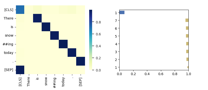
((a)) Attention map (left); Barcode (right); [L: $1$; H: $11$].

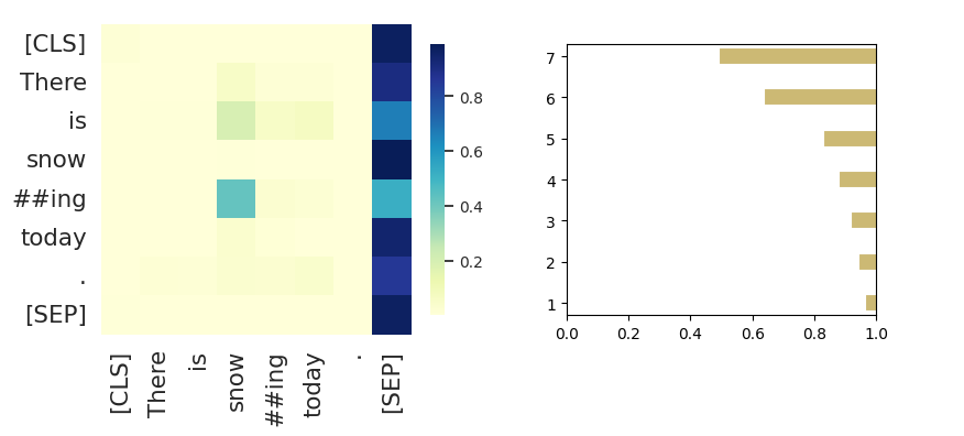
((b)) Attention map (left); Barcode (right); [L: $9$; H: $9$].

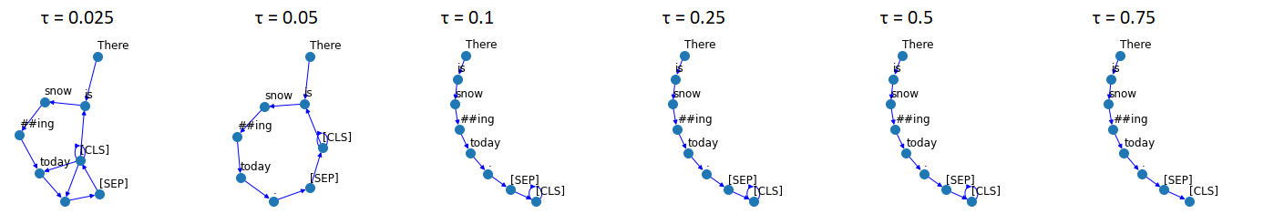
((c)) Attention graph filtration: [L: $1$; H: $11$].

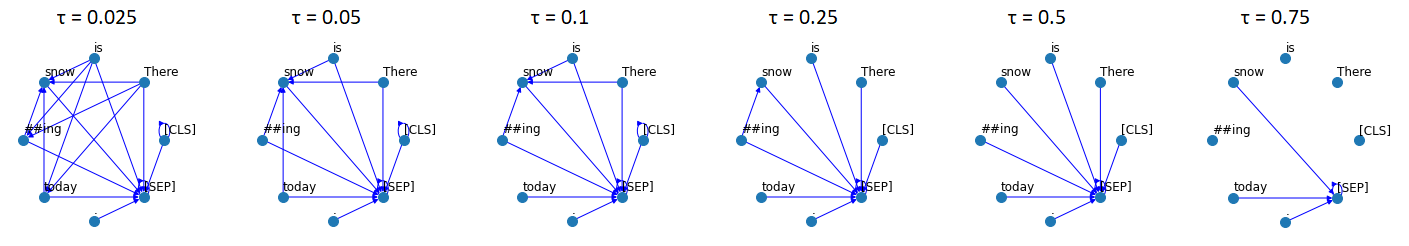
((d)) Attention graph filtration: [L: $9$; H: $9$].

Figure 1: An example of attention maps, barcodes, and filtration procedure for the sentence “There is snowing today.”. Model=En-BERT-base Devlin et al. (2019). Heads=[Layer $1$; Head $11$] and [Layer $9$; Head $9$].

3.1 Attention Graph

We treat Transformer’s attention matrix $A^{attn}$ as a weighted graph $G$, where the vertices represent tokens, and the edges connect pairs of tokens with mutual attention weights. This representation can be used to build a family of attention graphs called filtration, i.e., an ordered set of graphs $G^{\tau_{i}}$ filtered by increasing attention weight thresholds ${\tau_{i}}$. Filtering edges lower than the given threshold affects the graph structure and its core features, e.g., the number of edges, connected components, or cycles. TDA techniques allow tracking these changes, identifying the moments of when the features appear (i.e., their “birth”) or disappear (i.e., their “death”), and associating a lifetime to them. The latter is encoded as a set of intervals called a “barcode”, where each interval (“bar”) lasts from the feature’s “birth” to its “death”. The barcode characterizes the persistent features of attention graphs and describes their stability.

Example.

Let us illustrate the process of computing the attention graph filtration and barcodes given an Example 3.1. . There is snowing today.

First, we compute attention maps for each Transformer head as shown in 1(a)-1(b) (left). These two heads follow different attention patterns Clark et al. (2019): attention to the next token (Figure 1(a)) and to the [SEP] token (1(b)). Next, we represent the map as a weighted graph, and conduct the filtration procedure for a fixed set of attention weight thresholds. The edges lower than each given threshold are discarded, which results in a set of six attention graphs with their maximum spanning trees (MSTs) becoming a chain (1(c); $\tau$=$0.1$), and a star (1(d); $\tau$=$0.5$). The families of attention graphs are used to compute persistent features (§3.2).

1(a)-1(b) (right) depict barcodes for each family of graphs. The bars are sorted by length. The number of bars equals $|T|-1$, where $|T|$ is the number of tokens in the input sentence. The bars in yellow correspond to the $0$-dimensional features acquired from the edges of the MST. The bars in blue refer to $1$-dimensional features, which stand for non-trivial simple cycles. Such cycle appears in the first family (1(c); $\tau$=$0.05$), which is shown as a blue bar in 1(a). By contrast, there are no cycles in the second family (1(d)) and on the corresponding barcode.

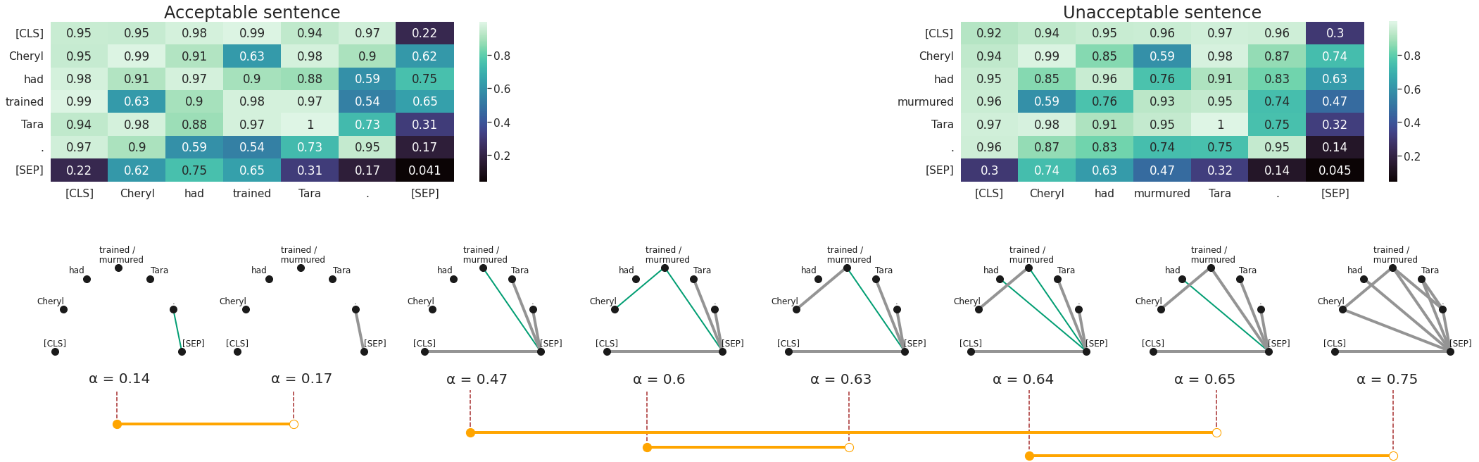
Figure 2: A graphical representation of RTD-barcodes. In the top row given $A^{\prime}$ matrices derived from attention maps for acceptable and unacceptable sentences. Edges present in both graphs $G_{a}^{\alpha_{i}}$ and $G_{b}^{\alpha_{i}}$ at a given threshold ${\alpha_{i}}$ are colored in grey. Edges present only in graph $G_{b}^{\alpha_{i}}$ are colored in green.

3.2 Persistent Features of Attention Graphs

We follow Kushnareva et al. (2021) to design three groups of persistent features of the attention graph: (i) topological features, (ii) features derived from barcodes, and (iii) features based on distance to attention patterns. The features are computed on attention maps produced by a Transformer LM.

Topological Features.

Topological features include the first two Betti numbers of the undirected graph $\beta_{0}$ and $\beta_{1}$ and standard properties of the directed graph, such as the number of strongly connected components, edges, and cycles. The features are calculated on pre-defined thresholds over undirected and directed attention graphs from each head separately and further concatenated.

Features Derived from Barcodes.

Barcode is the representation of the graph’s persistent homology Barannikov (2021). We use the Ripser++ toolkit Zhang et al. (2020) to compute $0$/$1$-dimensional barcodes for $A^{attn}$. Since Ripser++ leverages upon distance matrices, we transform $A^{attn}$ as $A^{\prime}=1-\max{(A^{attn},A^{attn~{}T})}$.

Next, we compute descriptive characteristics of each barcode, such as the sum/average/variance of lengths of bars, the number of bars with the time of birth/death greater/lower than a threshold, and the entropy of the barcodes. The sum of lengths of bars ($H_{0}S$) corresponds to the $0$-dimensional barcode and represents the sum of edge weights in the $A^{\prime}$’s minimum spanning tree. The average length of bars ($H_{0}M$) corresponds to the mean edge weight in this tree, i.e. $H_{0}M=1-$(the mean edge weight of the maximum spanning tree in $A^{attn}$ ).

Features Based on Distance to Patterns.

The shape of attention graphs can be divided into several patterns: attention to the previous/current/next token, attention to the [SEP]/[CLS] token, and attention to punctuation marks Clark et al. (2019). We formalize attention patterns by binary matrices and calculate distances to them as follows. We take the Frobenius norm of the difference between the matrices normalized by the sum of their norms. The distances to patterns are used as a feature vector.

Notations.

We summarize the notations used throughout the paper:

• $H_{i}$: $i$-th Homology Group

• $\beta_{i}$: Betti number, dimension of $H_{i}$

• $H_{0}S$: The sum of lengths of bars

• $H_{0}M$: The average of lengths of bars

• $PCA$: Principal Component Analysis

• $PC^{\{i\}}$: Subset $\{i\}$ of principal components

• $MST$: Maximum Spanning Tree

• RTD: Representation Topology Divergence

3.3 Representation Topology Divergence

Representation Topology Divergence (RTD; Barannikov et al., 2022) measures topological dissimilarity between a pair of weighted graphs with one-to-one vertex correspondence. Figure 2 outlines computation of RTD for a sentence pair in Example 3.3.

. . Cheryl had trained Tara. .̱ * Cheryl had murmured Tara.

First, we compute attention maps for the input sentences $S_{a}$ and $S_{b}$ with a Transformer LM, and represent them as the weighted graphs $G_{a}$ and $G_{b}$. Next, we establish a one-to-one match between the vertices, and sort the filtrations $G_{a}^{\alpha_{i}}$ and $G_{b}^{\alpha_{i}}$ with $\alpha$=$1-\tau$ in the ascending order. We then track the hierarchical formation of connected components in the graph $G_{a}^{\alpha_{i}}\cap G_{b}^{\alpha_{i}}$ while increasing $\alpha_{i}$. The RTD$(G_{a},~{}G_{b})$ feature appears at threshold $\alpha_{i}$ if an edge with the weight $\alpha_{i}$ in the graph $G_{b}$ joins two different connected components of the graph $G_{a}^{\alpha_{i}}\cap G_{b}^{\alpha_{i}}$. This feature disappears at the threshold $\alpha_{j}$ if the two $G_{a}^{\alpha_{i}}\cap G_{b}^{\alpha_{i}}$ connected components become joined in the graph $G_{a}^{\alpha_{j}}$.

Example.

We can identify the “birth” of the RTD feature at $\alpha$=$0.47$, when an edge appears in $G_{b}^{\alpha=0.47}$ between the connected component “trained/murmured” and the connected component with four vertices, namely “[SEP]”, “[CLS]”, “.”, and “Tara” (Figure 2; the appearing edge is colored in green). We observe its “death”, when the edge becomes present in both attention graphs at $\alpha$=$0.65$ (the corresponding edge changes its color to grey in the graph $G_{a}^{\alpha=0.65}\cap G_{b}^{\alpha=0.65}$). When comparing the graphs in this manner, we can associate a lifetime to the feature by computing the difference between the moments of its “death” (e.g., $\alpha_{j}$=$0.65$) and “birth” (e.g., $\alpha_{i}$=$0.47$). The lifetimes are illustrated as the orange bars $[\alpha_{i},\alpha_{j}]$ in Figure 2. The resulting value of RTD$(G_{a},~{}G_{b})$ is the sum of lifetimes $\alpha_{j}-\alpha_{i}$ over all such features. A formal description of RTD is provided in Appendix A.

4 Acceptability Classification

4.1 Data

We use three LA classification benchmarks in English (CoLA; Warstadt et al., 2019), Italian (ItaCoLA; Trotta et al., 2021) and Swedish (DaLAJ; Volodina et al., 2021). CoLA and ItaCoLA contain sentences from linguistic textbooks and cover morphological, syntactic, and semantic phenomena. The target labels are the original authors’ acceptability judgments. DaLAJ includes L2-written sentences with morphological violations or incorrect word choices. The benchmark statistics are described in Table 1 (see Appendix C). We provide examples of acceptable and unacceptable sentences in English subsection 4.1, Italian subsection 4.1, and Swedish subsection 4.1 from the original papers.

. . What did Betsy paint a picture of? .̱ *Maryann should leaving.

. . Ho voglia di salutare Maria.
“I want to greet Maria.” .̱ *Questa donna mi hanno colpito.
“This woman have impressed me.”

. . Jag kände mig jättekonstig.
“I felt very strange.” .̱ *Alla blir busiga med sociala medier.
“Everyone is busy with social media.”

4.2 Models

We run the experiments on the following Transformer LMs: En-BERT-base Devlin et al. (2019), It-BERT-base Schweter (2020), Sw-BERT-base Malmsten et al. (2020), and XLM-R-base Conneau et al. (2020). Each LM has two instances: frozen (a pre-trained model with frozen weights), and fine-tuned (a model fine-tuned for LA classification in the corresponding language).

Baselines.

We use the fine-tuned LMs, and a linear layer trained over the pooler output from the frozen LMs as baselines.

Our Models.

We train Logistic Regression classifiers over the persistent features computed with each model instance: (i) the average length of bars ($H_{0}M$); (ii) concatenation of all topological features referred to as TDA (§3.2). Following Warstadt et al., we evaluate the performance with the accuracy score (Acc.) and Matthew’s Correlation Coefficient (MCC; Matthews, 1975). The fine-tuning details are provided in Appendix B.

4.3 Results

Model	Frozen LMs		Fine-tuned LMs
	IDD / Dev	OODD / Test	IDD / Dev	OODD / Test
	Acc.   MCC	Acc.   MCC	Acc.   MCC	Acc.   MCC
CoLA
En-BERT	69.6   0.037	69.0   0.082	83.1   0.580	81.0   0.536
En-BERT + $H0M$	75.0   0.338	75.2   0.372	85.2   0.635	81.2   0.542
En-BERT + TDA	77.2   0.420	76.7   0.420	88.6   0.725	82.1   0.565
XLM-R	68.9   0.041	68.6   0.072	80.8   0.517	79.3   0.489
XLM-R + $H0M$	71.3   0.209	69.8   0.187	81.2   0.532	77.7   0.445
XLM-R + TDA	73.0   0.336	70.3   0.297	86.9   0.683	80.4   0.522
ItaCoLA
It-BERT	81.1   0.032	82.1   0.140	87.4   0.351	86.8   0.382
It-BERT + $H0M$	85.0   0.124	83.6   0.055	87.0   0.361	85.7   0.370
It-BERT + TDA	89.2   0.478	85.8   0.352	91.1   0.597	86.4   0.424
XLM-R	85.4   0.000	84.2   0.000	85.7   0.397	85.6   0.434
XLM-R + $H0M$	84.7   0.095	83.3   0.072	86.9   0.370	86.6   0.397
XLM-R + TDA	88.3   0.411	84.4   0.208	92.8   0.683	86.1   0.398
DaLAJ
Sw-BERT	58.3   0.183	59.0   0.188	71.9   0.462	74.2   0.500
Sw-BERT + $H0M$	69.3   0.387	58.4   0.169	76.9   0.542	68.7   0.375
Sw-BERT + TDA	62.1   0.243	64.4   0.289	71.8   0.442	73.4   0.478
XLM-R	52.2   0.069	51.5   0.038	60.6   0.243	62.8   0.297
XLM-R + $H0M$	61.1   0.224	61.8   0.237	62.5   0.256	64.5   0.295
XLM-R + TDA	51.1   0.227	54.1   0.218	62.5   0.255	65.5   0.322

Table 1: Acceptability classification results by benchmark. IDD=“in domain dev” set (CoLA). OODD=“out of domain dev” set (CoLA). Dev; Test=dev and test sets in ItaCoLA and DaLAJ. The best score is put in bold, the second best score is underlined.

Table 1 outlines the LA classification results. Our TDA classifiers generally outperform the baselines by up to $0.14$ MCC for English, $0.24$ MCC for Italian, and $0.08$ MCC for Swedish. The $H_{0}M$ feature can solely enhance the performance for English and Italian up to $0.1$, and concatenation of all features receives the best scores. Comparing the results under the frozen and fine-tuned settings, we draw the following conclusions. The TDA features significantly improve the frozen baseline performance but require the LM to be fine-tuned for maximizing the performance. However, the TDA/$H_{0}M$ classifiers perform on par with the fine-tuned baselines for Swedish. The results suggest that our features may fail to infer lexical items and word derivation violations peculiar to the DaLAJ benchmark.

Figure 3: Performance (MCC) of the fine-tuned En-BERT and XLM-R by major linguistic feature. Average MCC scores are represented with dashed lines. The number of sentences including the feature is placed in square brackets.

Effect of Freezing Layers.

Another finding is that freezing the Transformer layers significantly affects acceptability classification. Most of the frozen baselines score less than $0.1$ MCC across all languages. The results align with Lee et al. (2019), who discuss the performance degradation of BERT-based models depending upon the number of frozen layers. With all layers frozen, the model performance can fall to zero.

Results by Linguistic Features.

We run a diagnostic evaluation of the fine-tuned models using a grammatically annotated version of the CoLA development set Warstadt and Bowman (2019). Figure 3 (En-BERT and XLM-R; Figure 1 in Appendix C.1) present the results of measuring the MCC of the sentences including the major features.

The overall pattern is that the TDA classifiers may outperform the fine-tuned baselines, while the $H_{0}M$ ones perform on par with the latter. The performance is high on sentences with default syntax (Simple) and marked argument structure, including prepositional phrase arguments (Arg. Type), and verb phrases with unusual structures (Arg. Altern). The TDA features capture surface properties, such as presence of auxiliary or modal verbs (Auxiliary), and structural ones, e.g., embedded complement clauses (Comp Clause) and infinitive constructions (to-VP). The models receive moderate MCC scores on sentences with question-like properties (Question), adjuncts performing semantic functions (Adjunct), negative polarity items, and comparative constructions (Determiner).

Analysis of the Feature Space.

The LA classification experiments are conducted in the sparse feature space, where the TDA features can strongly correlate with one another, and their contribution is unclear. We run a complementary experiment to understand better how linguistic features are modeled with topology. We investigate the feature space with dimensionality reduction (principal component analysis, PCA; Pearson, 1901) by interpreting components’ structure and identifying the feature importance to the classifier’s predictions using Shapley values Shapley (1953), a game-theoretic approach to the attribution problem Sundararajan and Najmi (2020). Appendix C.2 describes the experiment on the fine-tuned En-BERT + TDA model using the grammatically annotated CoLA development set.

The results show that (i) features of the higher-layer heads, such as the average vertex degree, the number of connected components, edges, and cycles, and attention to the current token, contribute most to the major linguistic features. (ii) Attention to the [CLS]/next token is important to the Determiner, Arg. Type, Comp Clause, and to-VP properties, while attention to the first token and punctuation marks has the least effect in general. (iii) The number of nodes influences the classifier behavior, which is in line with Warstadt and Bowman, who discuss the effect of the sentence length on the performance.

5 Linguistic Minimal Pairs

5.1 Data

BLiMP (Benchmark of Linguistic Minimal Pairs; Warstadt et al., 2020a) evaluates the sensitivity of LMs to acceptability contrasts in terms of a forced choice between minimal pairs, as in Example 5.1. The benchmark consists of $67$ pair types, each including $1$k pairs covering $12$ language phenomena in morphology, syntax, and semantics.

. . Whose hat should Tonya wear? .̱ *Whose should Tonya wear hat?

5.2 Models

We conduct the experiments using two Transformer LMs for English: BERT-base and RoBERTa-base Liu et al. (2019).

Baselines.

We compare our methods with the results on BLiMP for human annotators and nine LMs Warstadt et al. (2020a); Salazar et al. (2020). The baselines range from statistical N-gram LMs to Transformer LMs.

Our Models.

Given a minimal pair as in Example 3.3, we build attention graphs $G_{a}$ and $G_{b}$ from each attention head of a frozen Transformer LM. We use the $H_{0}M$ feature (§3.2) and RTD (§3.3) as scoring functions to distinguish between the sentences $S_{a}$ and $S_{b}$. The scoring is based on empirically defined decision rules modeled after the forced-choice task:

• $H_{0}M$ scoring: $S_{a}$ is acceptable if and only if $H_{0}M(G_{a})~{}<~{}H_{0}M(G_{b})$; otherwise $S_{b}$ is acceptable.

• RTD scoring: $S_{a}$ is acceptable if and only if RTD$(G_{a},~{}G_{b})~{}<~{}$RTD$(G_{b},~{}G_{a})$; otherwise $S_{b}$ is acceptable.

We evaluate the scoring performance of each attention head, head ensembles, and all heads w.r.t. each and all linguistic phenomena in BLiMP. The following head configurations are used for each Transformer LM and scoring function:

Model	Overall	Ana. agr	Arg. str	Binding	Ctrl./rais.	D-N agr	Ellipsis	Filler	Irreg.	Island	NPI	Quant.	S-V agr
Warstadt et al. (2020a)
$5$-gram	61.2	47.9	71.9	64.4	68.5	70.0	36.9	60.2	79.5	57.2	45.5	53.5	60.3
LSTM	69.8	91.7	73.2	73.5	67.0	85.4	67.6	73.9	89.1	46.6	51.7	64.5	80.1
Transformer-XL	69.6	94.1	72.2	74.7	71.5	83.0	77.2	66.6	78.2	48.4	55.2	69.3	76.0
GPT2-large	81.5	99.6	78.3	80.1	80.5	93.3	86.6	81.3	84.1	70.6	78.9	71.3	89.0
Human Baseline	88.6	97.5	90.0	87.3	83.9	92.2	85.0	86.9	97.0	84.9	88.1	86.6	90.9
Salazar et al. (2020)
GPT2-medium	82.6	99.4	83.4	77.8	83.0	96.3	86.3	81.3	94.9	71.7	74.7	74.1	88.3
BERT-base	84.2	97.0	80.0	82.3	79.6	97.6	89.4	83.1	96.5	73.6	84.7	71.2	92.4
BERT-large	84.8	97.2	80.7	82.0	82.7	97.6	86.4	84.3	92.8	77.0	83.4	72.8	91.9
RoBERTa-base	85.4	97.3	83.5	77.8	81.9	97.0	91.4	90.1	96.2	80.7	81.0	69.8	91.9
RoBERTa-large	86.5	97.8	84.6	79.1	84.1	96.8	90.8	88.9	96.8	83.4	85.5	70.2	91.4
BERT-base + $H_{0}M$
[Layer; Head]	✗	[8; 8]	[8; 0]	[7; 0]	[8; 0]	[7; 0]	[7; 11]	[9; 7]	[6; 1]	[11; 7]	[8; 9]	[3; 7]	[8; 0]
Phenomenon Head	81.7	94.9	75.9	80.4	79.2	96.7	89.1	75.9	93.0	70.5	84.6	81.2	82.1
Top Head [8; 0]	75.4	86.8	75.9	63.4	79.2	83.7	72.2	67.3	90.3	70.0	83.1	63.5	82.1
Head Ensemble	84.3	93.3	79.9	83.5	78.6	96.4	78.4	79.5	93.8	74.4	92.5	81.7	86.8
All Heads	64.8	79.6	69.1	63.9	62.6	86.2	70.7	47.3	90.7	49.5	61.1	50.0	72.0
BERT-base + RTD
[Layer; Head]	✗	[8; 3]	[8; 0]	[7; 0]	[8; 0]	[7; 0]	[7; 11]	[9; 7]	[6; 1]	[9; 7]	[8; 9]	[3; 7]	[8; 0]
Phenomenon Head	81.8	94.5	75.8	80.4	79.2	96.7	89.1	75.0	93.0	72.2	84.4	81.2	82.0
Top Head [8; 0]	75.4	86.8	75.8	63.3	79.2	83.6	72.1	67.3	90.2	70.2	83.1	63.6	82.0
Head Ensemble	85.8	93.9	82.5	85.6	77.0	96.3	88.1	80.7	95.7	77.0	92.5	83.8	88.9
All Heads	65.3	77.8	68.5	63.2	63.6	86.0	73.4	48.4	91.0	51.3	62.0	51.2	72.6
RoBERTa-base + $H_{0}M$
[Layer; Head]	✗	[9; 5]	[9; 8]	[9; 5]	[9; 6]	[9; 0]	[8; 4]	[11; 10]	[9; 6]	[3; 5]	[11; 5]	[11; 3]	[8; 9]
Phenomenon Head	86.5	97.6	79.9	90.5	80.7	91.6	89.9	87.1	95.9	78.9	91.1	83.4	90.2
Top Head [11; 10]	81.9	90.1	66.0	84.7	71.7	91.0	86.7	87.1	89.5	76.8	90.7	78.4	85.0
Head Ensemble	87.8	96.3	79.6	87.6	82.6	93.6	84.9	90.4	94.3	83.0	94.6	80.6	92.8
All Heads	74.3	80.6	71.2	78.6	67.8	90.6	89.9	75.5	65.1	73.4	65.1	57.0	75.6
RoBERTa-base + RTD
[Layer; Head]	✗	[9; 5]	[9; 8]	[9; 5]	[9; 6]	[9; 0]	[8; 4]	[11; 10]	[2; 9]	[3; 5]	[10; 2]	[11; 3]	[9; 5]
Phenomenon Head	86.8	97.6	80.7	90.3	80.7	91.9	90.4	86.8	95.9	78.9	91.3	82.9	90.4
Top Head [11; 10]	80.8	88.8	63.3	83.7	69.8	90.2	88.8	86.8	89.1	76.5	89.0	78.4	83.1
Head Ensemble	88.9	97.0	83.3	86.9	81.6	93.7	88.1	88.8	95.5	83.0	94.2	84.2	92.7
All Heads	74.3	81.1	66.6	76.8	65.2	89.9	91.1	74.6	63.3	74.1	63.2	56.9	74.9

Table 2: Percentage accuracy of the baseline models, human baseline, and our methods on BLiMP. Overall is the average across all phenomena. The best score is put in bold, the second best score is underlined.

• Phenomenon Head and Top Head are the best-performing attention heads for each and all phenomena, respectively. The heads undergo the selection with a brute force search and operate as independent scorers.

• Head Ensemble is a group of the best-performing attention heads selected with beam search. The size of the group is always odd. We collect majority vote scores from attention heads in the group.

• All Heads involves majority vote scoring with all $144$ heads. We use random guessing in case of equality of votes. This setup serves as a proxy for the efficiency of the head selection.

Notes on Head Selection.

Recall that the head selection procedure imposes the following limitation. Auxiliary labeled minimal pairs are required to find the best-performing Phenomenon, Top Heads, and Head Ensembles. However, this procedure is more optimal and beneficial than All Heads since it maximizes the performance when utilizing only one or $9$-to-$59$ heads. We also analyze the effect of the amount of auxiliary data used for the head selection on the scoring performance (§5.3). Appendix D.1 presents a more detailed description of the head selection procedure.

5.3 Results

We provide the results of scoring BLiMP pairs in Table 2. The accuracy is the proportion of the minimal pairs in which the method prefers an acceptable sentence to an unacceptable one. We report the maximum accuracy scores for our methods across five experiment restarts. The general trends are that the best head configuration performs on par with the human baseline and achieves the highest overall performance (RoBERTa-base + RTD; Head Ensemble). RoBERTa predominantly surpasses BERT and other baselines, and topological scoring may improve on scores from both BERT and RoBERTa for particular phenomena.

Top Head Results.

We find that $H_{0}M$/RTD scoring with only one Top Head overall outperforms majority voting of $144$ heads (All Heads) by up to $10.6$% and multiple baselines by up to $20.7$% ($5$-gram, LSTM, Transformer-XL, GPT2-large). However, this head configuration performs worse than masked LM scoring Salazar et al. (2020) for BERT-base (by $8.8$%; Top Head=[$8$; $0$]) and RoBERTa-base (by $4.6$%; Top Head=[$11$; $10$]).

Phenomenon Head Results.

We observe that the $H_{0}M$/TDA scoring performance of Phenomenon Heads insignificantly differ for the same model. Phenomenon Heads generally receive higher scores than the corresponding Top Heads for BERT/RoBERTa (e.g., Binding: +$17.1$/+$5.8$%; Quantifiers: +$17.7$/+$5.0$%; Det.-Noun agr: +$13.0$/+$1.7$%), and perform best or second-best on Binding and Ellipsis. Their overall performance further adds up to $6.4$/$6.0$% and is comparable with Salazar et al.. The results indicate that heads encoding the considered phenomena are distributed at the same or nearby layers, namely $[3;$ $6$-$9;11]$ (BERT), and $[2$-$3;8$-$11]$ (RoBERTa).

BERT-base	RoBERTa-base

Table 3: Results of selecting the best-performing Head Ensembles with $H_{0}M$/RTD-based scoring. $H_{0}M$ heads are colored in green; RTD heads are colored in yellow.

Head Ensemble Results.

Table 3 describes the most optimal Head Ensembles by Transformer LM. Most heads selected under the $H_{0}M$ and RTD scoring functions are similar w.r.t. LMs. While the selected BERT heads are distributed across all layers, the RoBERTa ones tend to be localized at the middle-to-higher layers. Although RoBERTa utilizes smaller ensembles when delivering the best overall score, some heads contribute in both LMs, most notably at the higher layers.

Overall, the RoBERTa $H_{0}M$/RTD ensembles get the best results on Filler gap, Quantifiers, Island effects, NPI, and S-V agr as shown in Table 2, matching the human level and surpassing four larger LMs on all phenomena by up to $7.4$% (GPT2-medium and GPT2/BERT/RoBERTa-large).

Effect of Auxiliary Data.

Note that the head selection can be sensitive to the number of additional examples. The analysis of this effect is presented in Appendix D.2. The results show that head ensembles, their size, and average performance tend to be more stable when using sufficient examples (the more, the better); however, using only one extra example can yield the performance above $80$%.

6 Discussion

Topology and Acceptability. The topological properties of the attention graph represent interpretable and versatile features for judging sentence acceptability and identifying acceptability contrasts in minimal pairs. As one of such properties, the sum length of bars ($H_{0}S$) — and its normalized version ($H_{0}M$) — have proved to be efficient for both LA approaches. This simple feature can serve as a profitable input for LA classifiers and a scoring function to discriminate between minimal pairs. Figure 4 shows an example of the $H_{0}S$ sensitivity to CoLA’s question-like properties, such as wh-movement out of syntactic islands and matrix and embedded questions. We provide more examples in Appendix E, which demonstrate the distribution shifts between the acceptable and unacceptable sentences.

Acceptability Phenomena.

The underlying structure of the attention graph encodes various well-established grammatical concepts. We observe that the persistent graph features capture surface properties, morphological agreement, structural relationships, and simple/complex syntactic phenomena well. However, with topology, lexical items, optional syntactic elements, and abstract semantic factors may be difficult to infer. Attention to the first token and punctuation marks contribute least to LA classification, while the other attention pattern features capture various phenomena.

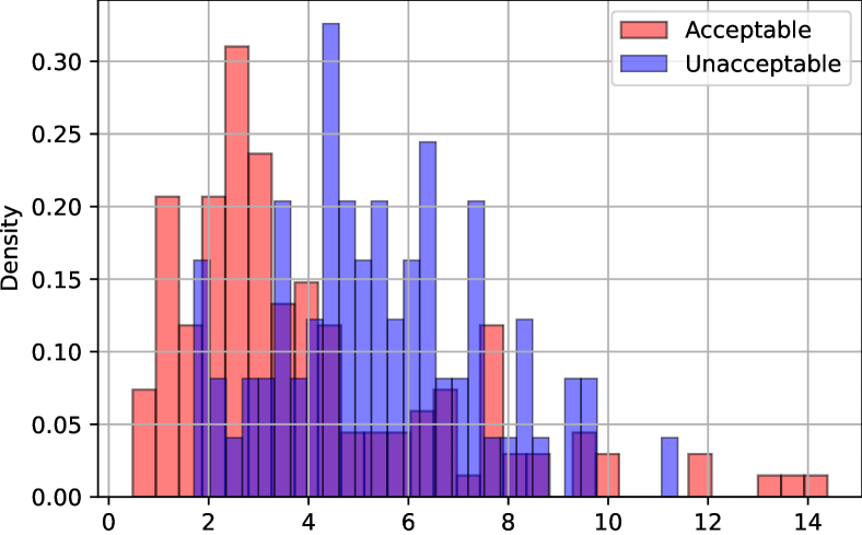
Figure 4: The distribution shift of the $H_{0}S$ feature between the acceptable and unacceptable sentences (Question); [L: $10$; H: $0$].

Linguistic Roles of Heads.

Topological tools help gain empirical evidence about the linguistic roles of heads from another perspective. Our findings on the heads’ roles align with several related studies. The results on the CoLA-style and BLiMP benchmarks indicate that (i) a single head can perform multiple linguistic functions Pande et al. (2021), (ii) some linguistic phenomena, e.g., phrasal movement and island effects, are better captured by head ensembles rather than one head Htut et al. (2019), and (iii) heads within the same or nearby layers extract similar grammatical phenomena Bian et al. (2021).

7 Conclusion and Future Work

Our paper studies the ability of attention heads to judge grammatical acceptability, demonstrating the profitable application of TDA tools to two LA paradigms. Topological features can boost LA classification performance in three typologically close languages. The $H_{0}M$/RTD scoring matches or outperforms larger Transformer LMs and reaches human-level performance on BLiMP, while utilizing $9$-to-$59$ attention heads. We also interpret the correspondence between the persistent features of the attention graph and grammatical concepts, revealing that the former efficiently infer morphological, structural, and syntactic phenomena but may lack lexical and semantic information.

In our future work we hope to assess the linguistic competence of Transformer LMs on related resources for typologically diverse languages and analyze which language-specific phenomena are and are not captured by the topological features. We are also planning to examine novel features, e.g., the number of vertex covers, the graph clique-width, and the features of path homology Grigor’yan et al. (2020). Another direction is to evaluate the benefits and limitations of the $H_{0}M$/RTD features as scoring functions in downstream applications.

We also plan to introduce support for new deep learning frameworks such as MindSpore Tong et al. (2021) to bring TDA-based experimentation to the wider industrial community.

8 Limitations

8.1 Computational complexity

Acceptability classification. Calculation of any topological feature relies on the Transformer’s attention matrices. Hence, the computational complexity of our features is not lower than producing an attention matrix with one head, which is asymptotically $O(n^{2}d+nd^{2})$ given that $n$ is the maximum number of tokens, and $d$ is the token embedding dimension Vaswani et al. (2017).

The calculation complexity of the pattern-based and threshold-based features is done in linear time $O(e+n)$, where $e$ is the number of edges in the attention graph. In turn, the number of edges is not higher than $\frac{n(n-1)}{2}\sim n^{2}$. The computation of the 0^th Betti number $\beta_{0}$ takes linear time $O(e+n)$, as $\beta_{0}$ is equal to the number of the connected components in an undirected graph. The computation of the 1^st Betti number $\beta_{1}$ takes constant time, since $\beta_{1}=e-n+\beta_{0}$. The computational complexity of the number of simple cycles and the $1$-dimensional barcode features is exponential in the worst case. To reduce the computational burden, we stop searching for simple cycles after a pre-defined amount of them is found.

Note that the computational costs could be reduced, e.g., by identifying the most contributing features or the best-performing heads. Consider an example in Figure 5, which illustrates how the CoLA performance gets changed depending on the number of En-BERT heads. Here, the head selection is based on a simple procedure. First, we score the attention heads by calculating the maximum correlation between each head’s features and the vector of the target classes on the train set. Second, we train a linear classifier over the TDA features produced by $N$ attention heads ranked by the correlation values, as specified in §4.2. Satisfactory MCC scores can be achieved when utilizing less than $40$ heads with a significant speed up at the inference stage.

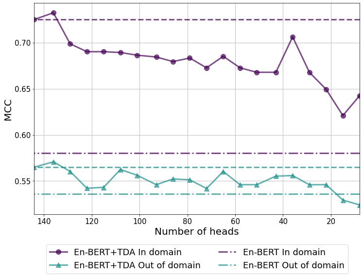
Figure 5: Performance on the CoLA development set depending on the number of heads for En-BERT + TDA.

Linguistic Minimal Pairs. Computation of the $H_{0}M$ and RTD features is run via the Ripser++ GPU library. Under this library, the minimum spanning tree is found according to Kruskal’s algorithm giving the computational complexity of $H_{0}M$ as $O(n^{2}\log n)$. The complexity can be reduced using other algorithms, e.g., Prim’s algorithm, which takes $O(n^{2})$. The RTD’s computational complexity is more difficult to estimate. RTD is computed via persistence barcodes of dimension 1 for a specific graph with $2n$ vertices. Many optimization techniques and heuristics are implemented in the Ripser++ library that significantly reduce the RTD’s complexity.

Empirical estimate.

Computing the $H_{0}M$/RTD features with $144$ BERT heads in the worst case of a $512$-token text takes $2.41$ and $94.5$ sec (NVIDIA Tesla K80 $12$GB RAM). However, the actual computation time on the considered tasks is empirically more optimal. We provide empirical estimates on the entire BLiMP and LA datasets: $2.4$/$15.7$ hours on BLiMP ($H_{0}M$/RTD) and up to $2$ hours on CoLA/ItaCoLA/DaLAJ (estimates by the feature groups: topological features=$24$%; features derived from barcodes=$70$%; and features based on distance to patterns=$6$% of the total time).

8.2 Application Limitations

We also outline several application limitations of our approach. (i) The LA classifiers require preliminary fine-tuning of Transformer LMs to extract more representative attention graph features and, therefore, achieve better performance. (ii) RTD operates upon a one-to-one vertex correspondence, which may be hindered by tokens segmented into an unequal amount of sub-tokens. As a result, identifying the topological discrepancy between pairs of attention graphs can be restricted in practice, where the graphs are of an arbitrary number of nodes. Regardless of the potential information loss due to sentence truncation in such cases, the RTD heads still receive the best overall score on BLiMP. (iii) The head selection procedure relies on auxiliary data to identify the best-performing head configurations. Annotating the auxiliary data may require additional resources and expertise for practical purposes. However, the procedure maximizes the performance and reduces the computational costs by utilizing less attention heads.

8.3 Linguistic Acceptability

Acceptability judgments have been broadly used to investigate whether LMs learn grammatical concepts central to human linguistic competence. However, this approach has several methodological limitations. (i) The judgments may display low reproducibility in multiple languages Linzen and Oseki (2018), and (ii) be influenced by an individual’s exposure to ungrammatical language use Dąbrowska (2010). (iii) Distribution shifts between LMs’ pre-training corpora and LA datasets may introduce bias in the evaluation since LMs tend to assign higher probabilities to frequent patterns and treat them as acceptable in contrast to rare ones Marvin and Linzen (2018); Linzen and Baroni (2021).

9 Ethical Statement

Advancing acceptability evaluation methods can improve the quality of natural language generation Batra et al. (2021). We recognize that this, in turn, can increase the misuse potential of such models, e.g., generating fake product reviews, social media posts, and other targeted manipulation Jawahar et al. (2020); Weidinger et al. (2021). However, the acceptability classifiers and scoring functions laid out in this paper are developed for research purposes only. Recall that the topological tools can be employed to develop adversarial defense and artificial text detection models for mitigating the risks Kushnareva et al. (2021).

Appendix A Representation Topology Divergence

Suppose we have two weighted full graphs $G_{a},G_{b}$ with one-to-one vertex correspondence. Define their vertices as $\{a_{1},a_{2},\ldots,a_{n}\}$ and $\{b_{1},b_{2},\ldots,b_{n}\}$ respectively so that $a_{i}$ corresponds to $b_{i}$ for each $i$. RTD($G_{a},G_{b}$) is calculated as follows:

1. Build a full weighted graph $G_{ab}$ with the vertices set $V=\{v_{1},v_{2},\ldots v_{n},u_{1},u_{2},\ldots,u_{n}\}$ and the edge weights computed as

   $$\begin{cases}w(v_{i},v_{j})=0\\ w(v_{i},u_{i})=0\\ w(u_{i},u_{j})=w_{b}(b_{i},b_{j})\\ w(v_{i},u_{j})=\max{(w_{a}(a_{i},a_{j}),w_{b}(b_{i},b_{j}))}\\ \end{cases}$$

   where $w_{a}$ and $w_{b}$ are the edge weights in the corresponding graphs.

2. Compute the barcode Barannikov (2021) of the $H_{1}$ homology group of the graph $G_{ab}$ flag complex. It should be emphasized that the $H_{0}$ homology group barcode for this graph is empty since the minimum spanning tree of $G_{ab}$ has the total weight of $0$. Instead of $H_{1}$, the higher-order homology groups (e.g., $H_{2}$, $H_{3}$) can be considered. However, the preliminary experiments have shown that they are less helpful for LA tasks.

3. RTD$(G_{a},G_{b})$ is calculated as the sum of bar lengths in the barcode from the previous step.

It should be noted that this procedure is asymmetric on $G_{a}$ and $G_{b}$, and for non-equal graphs holds RTD$(G_{a},G_{b})\neq$ RTD$(G_{b},G_{a})$. To compute barcodes, we use the Ripser++ toolkit, which cannot work with asymmetric graphs. Hence, we represent the asymmetric attention maps as the distance matrices to obtain the symmetric graphs $G_{a}$ and $G_{b}$ as described in §3.2. We consider only the forward-looking part of attention, i.e., how each token affects the rest of the sentence.

The majority of the BLiMP minimal pairs are of equal length in the BERT/RoBERTa tokens. Otherwise, we truncate the longest sentence to achieve an equal length since the one-to-one correspondence between tokens is crucial for RTD. We assume that the truncation may remove tokens that help to discriminate between the acceptable and unacceptable sentences. We leave improvement of the pre-processing stage for future work.

Appendix B Fine-tuning Details

Fine-tuning and evaluation of the BERT-based/XLM-R acceptability classifiers follow the standard procedure under the HuggingFace library Wolf et al. (2020). Each model is fine-tuned for $4$ epochs with the learning rate of $1e^{-2}$/$1e^{-3}$, batch size of $32$, and the other default hyperparameters.

Appendix C Acceptability Classification

	CoLA	ItaCoLA	DaLAJ
Language	English	Italian	Swedish
# Train sent.	8,551	7,801	6,870
# Dev sent.	1,043	946	892
# Test sent.	1,063	975	952
Type	Expert	Expert	L2
# Sources	23	12	SweLL
Phenomena	Morph, Syntax, Semantics	Syntax	Lexis, Morph
%	70.5	84.5	50.0

Table 1: Statistics of acceptability classification benchmarks. Type=Type of data source. %=Percentage of acceptable sentences. Morph=Morphology.

C.1 Results by Linguistic Features

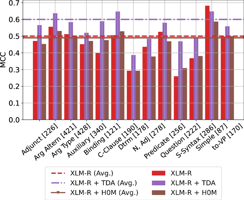
Figure 1: Performance (MCC) of the fine-tuned XLM-R by major linguistic feature. Average MCC scores are represented with dashed lines. The number of sentences including the feature is placed in square brackets.

C.2 Analysis of the Feature Space

We analyze the contribution of the topological features to acceptability classification in the context of linguistic phenomena. We interpret the principal components computed on the fine-tuned En-BERT + TDA features and identify their importance w.r.t. each head/layer with Shapley values.

Method. The pipeline assembles the feature standardization, PCA and training a logistic regression classifier. We conduct a grid search over two pipeline’s parameters (i) the number of components $N_{comp}\in[10,20,\dots,100]$ (the found optimum: $N_{comp}=100$) and (ii) regularization parameter of logistic regression $L_{1}\in[0.01,0.02,\dots,0.1]$ (the found optimum: $L_{1}=0.1$). The parameter search is run across $3$ stratified folds, where the CoLA train set is randomly split into train/development sets. The classifier performance is evaluated on the grammatically annotated CoLA development set. We also explore masking principal components, i.e., training the classifier using only the most important components while zeroing the weights of the others.

Table 2 shows results for the full pipeline (En-BERT + TDA + PCA) and masked pipelines (En-BERT + TDA + PC¹/PC²). Since the performance is comparable with the En-BERT + TDA classifier in §4, we rely on the PCA decomposition for the feature analysis and interpretation.

Model	IDD	OODD
	Acc.   MCC	Acc.   MCC
En-BERT + TDA	88.6   0.725	82.1   0.565
En-BERT + TDA + PCA	84.8   0.632	81.8   0.558
En-BERT + TDA + PC1	84.1   0.609	79.1   0.482
En-BERT + TDA + PC2	84.3   0.615	81.2   0.541

Table 2: Acceptability classification results with PCA on CoLA. IDD=“in domain dev” set. OODD=“out of domain dev” set. Components Set ¹: {1}, Components Set²: {1,7,9,24,12,0}.

Results. The following six principal components (PCs) contribute most to acceptability classification according to the mean absolute Shapley values $\phi$ (see Figure 2). Figure 3 shows the Shapley values for these PCs by the major linguistic feature.

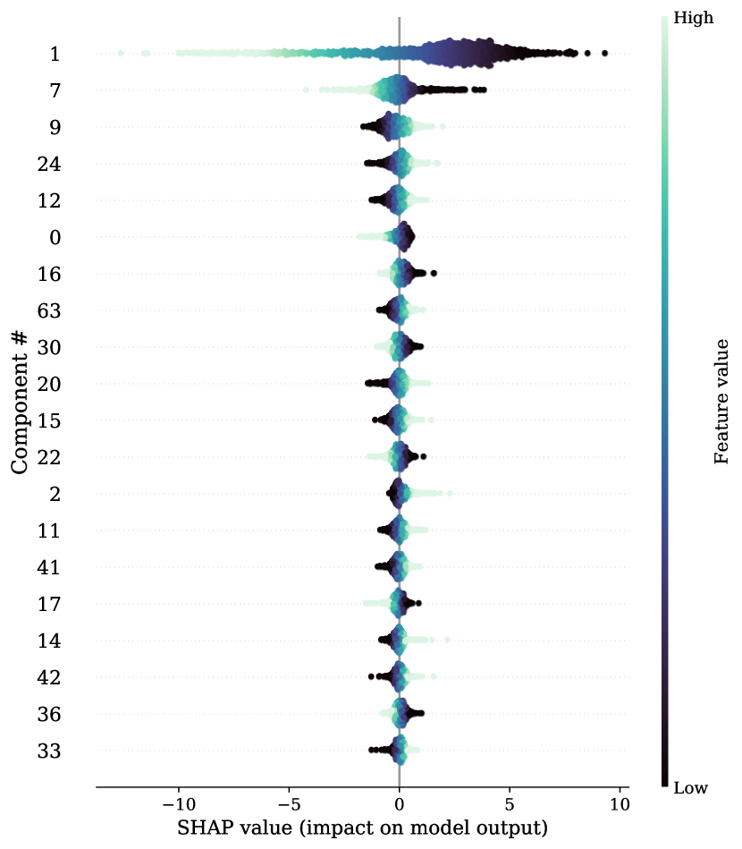
Figure 2: Importance of the PCs for judging sentence acceptability. Shapley values $\phi$ reflect the PCs’ impact on the classifier output.

PC1 ($\phi$=$3.179$) has the most impact on the classifiers’ performance. PC1 primarily contains simple topological features (the average vertex degree, the number of edges, and the number of connected components) from the heads at the last layer, which is affected most by the fine-tuning.

PC7 ($\phi$=$0.601$) includes same heads as PC1, but its features utilize the number of cycles in the attention graph.

PC9 ($\phi$=$0.442$) groups all attention patterns except for attention to commas for heads at the lower and middle layers. The component attributes to all phenomena.

PC24 ($\phi$=$0.296$) is responsible for topological features at the first and last layers.

PC12 ($\phi$=$0.278$) contains the attention to the [CLS] token/next token patterns. The PC is important for classifying sentences including the following features: negative polarity and free choice items (Determiner), obliques, expletives, prepositional phrases and arguments (Argument Type), complement clauses without complementizers (Complement Clause).

PC0 ($\phi$=$0.274$) represents features equal to the number of nodes in the graph, that is, the sentence length in tokens. The PC influences the classifier prediction w.r.t. most of the phenomena, except for Determiner, Complement Clause, and Argument Types.

The following four PCs are less important for acceptability classification ($\phi_{j}<0.25$) in general but may contribute to some linguistic phenomena.

PC16 ($\phi$=$0.243$) comprises topological and distance to pattern features of different heads at the middle layers. The PC contributes to negative polarity and free choice items, non-finite complementizer phrases, and comparative constructions.

PC20 ($\phi$=$0.216$) reflects attention-to-comma for various heads at the lower layers. However, this feature helps to classify sentences that fall under the S-Syntax and Question categories.

PC15 ($\phi$=$0.216$) includes the attention to the first token pattern for the middle-to-higher layer heads (generally 4-to-10). It works for Passive and By-Phrases.

PC2 ($\phi$=$0.203$) reflects the number of graph edges for heads at the first layer, which captures strong pair-wise information about tokens. This head is important for sentences with default syntax (Simple).

PC3 and PC6 ($\phi<0.05$) represent attention to the dot pattern. The PCs are not important for any of the linguistic phenomena and have large eigenvalues.

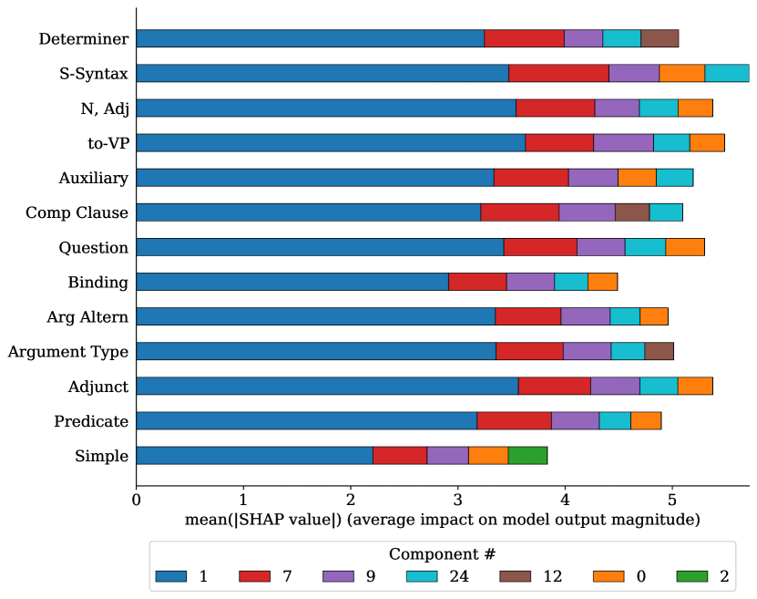
Figure 3: Concatenated mean absolute Shapley values for the important PCs by major linguistic feature.

Appendix D Attention Head Selection

D.1 Head Selection Procedure

We use publicly available scripts to generate up to $100$ minimal pairs per each of $67$ types, ensuring no overlap with the BLiMP pairs. We select the best-performing individual heads and head ensembles by estimating their scoring performance on the generated data and further evaluate them on BLiMP.

Algorithms 1-2 describe the Top Head and Phenomenon Head selection procedures using a brute force search, while Algorithm 3 presents the process of selecting the Head Ensembles via beam search.

Algorithm 1 Top Head Selection

Set $Q_{1}$: contains all possible pairs $(h,r)$, where $h$ – attention head and $r\in\{1,2\}$ – scoring rule

2:$acc(.):$ accuracy evaluation function of the head with the selected rule on pairs for all phenomenas

Pair $(H_{B},R_{B})$

4:procedure Selecting Top Head($Q_{1}$)

     $BestAcc\leftarrow 0$

6:     $(H_{B},R_{B})\leftarrow(-1,-1)$

     for $(h,r)\in Q_{1}$ do

8:         if $acc((h,r))>BestAcc$ then

              $BestAcc\leftarrow acc_{C}((h,r))$

10:              $(H_{B},R_{B})\leftarrow(h,r)$

         end if

12:     end for

     return: $(H_{B},R_{B})$

14:end procedure

Algorithm 2 Phenomenon Head Selection

Set $Q_{1}$: contains all possible pairs $(h,r)$, where $h$ – attention head and $r\in\{1,2\}$ – scoring rule

2:$C:$ linguistic category

$acc_{C}(.):$ accuracy evaluation function of the head with the selected scoring rule on the $C$ pairs

4:Pair $(H_{C},R_{C})$

procedure Selecting Phenomenon Head($Q_{1}$)

6:     $BestAcc\leftarrow 0$

     $(H_{C},R_{C})\leftarrow(-1,-1)$

8:     for $(h,r)\in Q_{1}$ do

         if $acc_{C}((h,r))>BestAcc$ then

10:              $BestAcc\leftarrow acc_{C}((h,r))$

              $(H_{C},R_{C})\leftarrow(h,r)$

12:         end if

     end for

14:     return: $(H_{C},R_{C})$

end procedure

Algorithm 3 Head Ensemble Selection

Set $Q_{1}$: contains all possible pairs $(h,r)$, where $h$ – attention head and $r\in\{1,2\}$ – scoring rule

2:$acc(.):$ accuracy evaluation function of the ensembles with selected scoring rules using majority voting

Ensemble $B$: set of pairs $(H,R)$

4:procedure Selecting Head Ensemble($Q_{1}$)

     $Q\leftarrow\{\{(h,r)\}\mid(h,r)\in Q_{1}\}$

6:     do

         $Q^{\prime}\leftarrow\emptyset$

8:         for $q\in Q$ do

              for $(h_{1},r_{1})\neq(h_{2},r_{2})\in Q_{1}\setminus q$ do

10:                  $q^{\prime}\leftarrow q\cup\{(h_{1},r_{1}),(h_{2},r_{2})\}$

                  if $acc(q^{\prime})>acc(q)$ then

12:                       $Q^{\prime}\leftarrow Q^{\prime}\cup\{q^{\prime}\}$

                  end if

14:              end for

         end for

16:         if $\rvert Q\lvert~{}\geq 40$ then

              $Q\leftarrow$ top-$40$ pairs $q$, scored by $acc(.)$, $q\in Q^{\prime}$

18:         else

              if $\rvert Q^{\prime}\lvert~{}>0$ then

20:                  $Q\leftarrow Q^{\prime}$

              end if

22:         end if

     while $Q^{\prime}\neq\emptyset$

24:     return: Ensemble from $Q$

end procedure

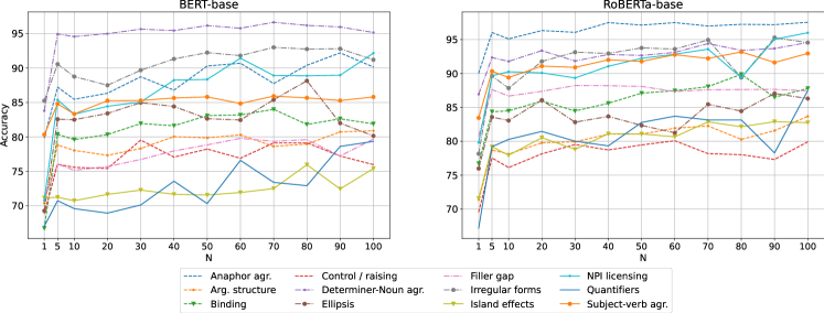
Figure 4: The effect of a given amount of examples on the BLiMP performance of selected Head Ensembles by major category. Method=RTD scoring. N=number of extra examples per phenomenon.

D.2 Effect of Auxiliary Data

We analyze the effect of the amount of auxiliary generated data on the RTD scoring performance. We explore $N\in[1,5,10,...,100]$ sentence pairs per language phenomenon used for selecting Head Ensembles as described in Appendix D.1. The experiments are run ten times, where each run includes generation of auxiliary minimal pairs, the corresponding head selection procedure, and evaluation on BLiMP for each and all language phenomena. The accuracy performance is averaged over all experiment runs.

Results. Figure 4 presents the results for the BERT-base and RoBERTa-base models. We observe that some phenomena receive prominent performance using only one auxiliary example (e.g., BERT-base: Irregular forms: $85\%$; Determiner-Noun agr: $84\%$; Anaphor agr: $80\%$; Subject-verb agr: $80\%$; RoBERTa-base: Anaphor agr: $90\%$; Determiner-Noun agr: $87\%$; Subject-verb agr: $83\%$). Both models receive similar maximum scores for some phenomena with a given different amount of examples (Control / raising: $79\%$/$80\%$, N=$30/60$; Ellipsis: $88\%$/$87\%$, N=$80/90$; Filler gap: $80\%$/$88\%$, N=$60/30$). By contrast, there is a significant difference between the maximum and minimum scores on certain phenomena, e.g., Quantifiers ($10\%$/$9\%$), NPI licensing ($8\%$/$6\%$), and Ellipsis ($8\%$/$6\%$).

Appendix E The $H_{0}S$ Feature Distributions

Figure 5 and Figure 6 illustrate examples of the $H_{0}S$ feature distribution shifts between the acceptable and unacceptable sentences from the entire CoLA development set.

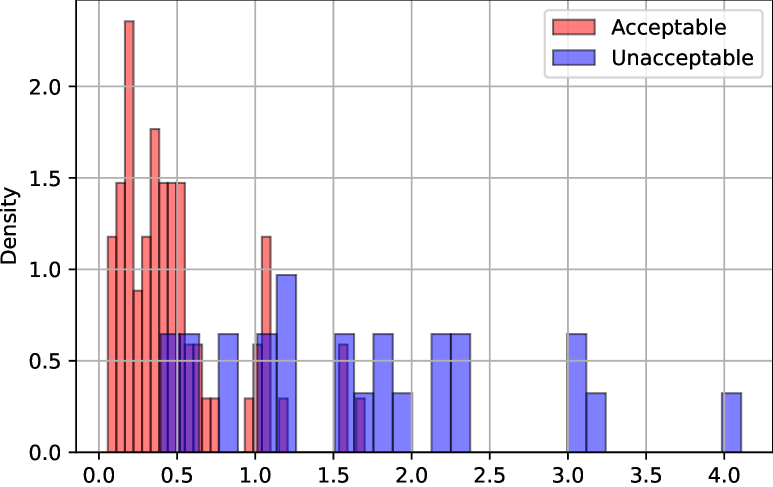
Figure 5: The distribution shift of the $H_{0}S$ feature between the acceptable and unacceptable sentences (Simple); [L: $10$; H: $3$].

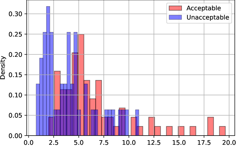
Figure 6: The distribution shift of the $H_{0}S$ feature between the acceptable and unacceptable sentences (Binding); [L: $11$; H: $4$].

Appendix F Toy Examples of Calculating Features

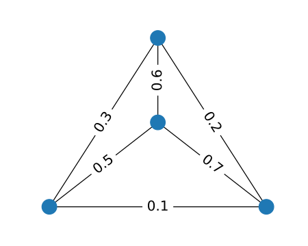
((a)) $G_{toy}$

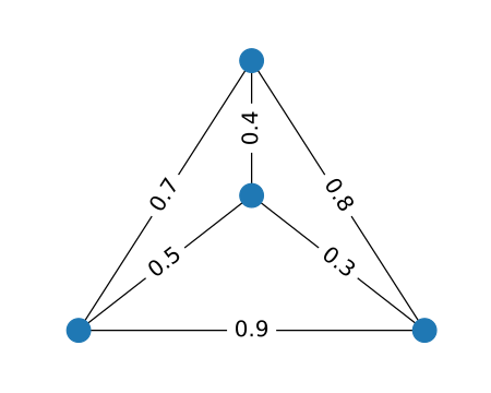
((b)) $G_{toy}^{\prime}$

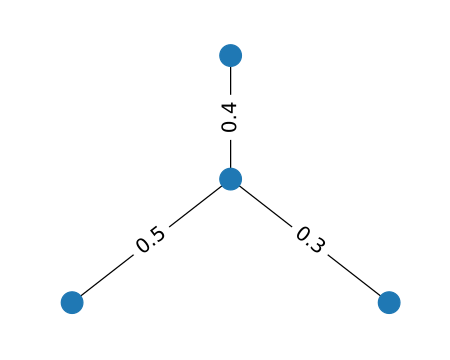
((c)) minimum spanning tree
of $G_{toy}^{\prime}$

((d)) $H_{0}$-barcode of $G^{\prime}_{toy}$

Figure 7: An example of a weighted graph and corresponding $H_{0}$-barcode, calculated with the Ripser++ library.

Let us demonstrate a calculation of essential barcode features of a toy graph $G_{toy}$ ( 7(a)). First, we calculate the $H_{0}$-barcode of this graph. To do it, we build the graph $G^{\prime}_{toy}$ by replacing each edge weight $w$ with $1-w$, as in 7(b). Next we calculate the minimum spanning tree of this new graph (7(c)). We end up with the $H_{0}$-barcode with the lengths of bars, equal to the weights of the minimum spanning tree (7(d)). We can derive $H_{0}S(G_{toy})=0.3+0.4+0.5=1.2$ and $H_{0}M(G_{toy})=H_{0}S(G_{toy})/3=0.4$ from this barcode diagram.

Note that the directions of the bars (Figure 1) were reversed comparing to the actual ripser++ output (7(d)). The reversed representation is more intuitive: edges with lower weights are filtered out earlier than edges with the higher weights.

Next we compute the Betti numbers for the same graph $G_{toy}$ given three thresholds: $\tau_{1}=0$, $\tau_{2}=0.4$ and $\tau_{3}=1$.

At $\tau=0$ we do not drop any edges. We have the full graph with one connected component (7(a)). $\beta_{0}$ is defined as the number of connected components. Hence $\beta_{0}$ equals to $1$. Next we calculate $\beta_{1}$, using the shortcut formula for graphs: $\beta_{1}=|E|+|C|-|V|$. In our case, $|E|=6$ is the number of edges, $|C|=1$ is the number of connected components and $|V|=4$ is the number of vertices. Finally, we get $\beta_{1}=3$. Note that $\beta_{1}$ corresponds to three simple undirected loops in the graph. There is also an alternative method to represent the graph and to calculate the first Betti number. This method does not account for “trivial” loops, which are defined by the triangles borders. It was used in the example above, see Figure 1.

At $\tau=0.4$, we drop all edges with weights lower than $0.4$. We get the same structure as the minimum spanning tree of the graph $G_{toy}^{\prime}$ (7(c)), but without weights inversion. For this graph, $\beta_{0}=1$: there is a single connected component, $\beta_{1}=3+1-4=0$. It corresponds to the number of simple loops, which equals to $0$.

At $\tau=1$, we drop all edges as all edges have weights below than $1$. The resulting graph consists only of vertices without edges. For this case, we have four connected components, so $\beta_{0}=4$, and $\beta_{1}=0+4-4=0$.

References

- Barannikov (1994) Serguei Barannikov. 1994. Framed Morse complexes and its invariants. Adv. Soviet Math., 21:93–115.
- Barannikov (2021) Serguei Barannikov. 2021. Canonical Forms = Persistence Diagrams. Tutorial. In European Workshop on Computational Geometry (EuroCG 2021).
- Barannikov et al. (2022) Serguei Barannikov, Ilya Trofimov, Nikita Balabin, and Evgeny Burnaev. 2022. Representation Topology Divergence: A Method for Comparing Neural Network Representations. In Proceedings of the 39th International Conference on Machine Learning, volume 162, pages 1607–1626. PMLR.
- Batra et al. (2021) Soumya Batra, Shashank Jain, Peyman Heidari, Ankit Arun, Catharine Youngs, Xintong Li, Pinar Donmez, Shawn Mei, Shiunzu Kuo, Vikas Bhardwaj, Anuj Kumar, and Michael White. 2021. Building adaptive acceptability classifiers for neural NLG. In Proceedings of the 2021 Conference on Empirical Methods in Natural Language Processing, pages 682–697, Online and Punta Cana, Dominican Republic. Association for Computational Linguistics.
- Bian et al. (2021) Yuchen Bian, Jiaji Huang, Xingyu Cai, Jiahong Yuan, and Kenneth Church. 2021. On attention redundancy: A comprehensive study. In Proceedings of the 2021 Conference of the North American Chapter of the Association for Computational Linguistics: Human Language Technologies, pages 930–945, Online. Association for Computational Linguistics.
- Burlot and Yvon (2017) Franck Burlot and François Yvon. 2017. Evaluating the morphological competence of machine translation systems. In Proceedings of the Second Conference on Machine Translation, pages 43–55, Copenhagen, Denmark. Association for Computational Linguistics.
- Carlsson and Vejdemo-Johansson (2021) Gunnar Carlsson and Mikael Vejdemo-Johansson. 2021. Topological Data Analysis with Applications. Cambridge University Press.
- Chazal and Michel (2017) Frédéric Chazal and Bertrand Michel. 2017. An Introduction to Topological Data Analysis: Fundamental and Practical Aspects for Data Scientists. arXiv preprint arXiv:1710.04019.
- Cherry and Quirk (2008) Colin Cherry and Chris Quirk. 2008. Discriminative, syntactic language modeling through latent SVMs. In Proceedings of the 8th Conference of the Association for Machine Translation in the Americas: Research Papers, pages 65–74, Waikiki, USA. Association for Machine Translation in the Americas.
- Chomsky (1965) Noam Chomsky. 1965. Aspects of the Theory of Syntax. MIT Press.
- Clark et al. (2013) Alexander Clark, Gianluca Giorgolo, and Shalom Lappin. 2013. Statistical representation of grammaticality judgements: the limits of n-gram models. In Proceedings of the Fourth Annual Workshop on Cognitive Modeling and Computational Linguistics (CMCL), pages 28–36, Sofia, Bulgaria. Association for Computational Linguistics.
- Clark et al. (2019) Kevin Clark, Urvashi Khandelwal, Omer Levy, and Christopher D. Manning. 2019. What does BERT look at? an analysis of BERT’s attention. In Proceedings of the 2019 ACL Workshop BlackboxNLP: Analyzing and Interpreting Neural Networks for NLP, pages 276–286, Florence, Italy. Association for Computational Linguistics.
- Colombo et al. (2021) Pierre Colombo, Guillaume Staerman, Chloé Clavel, and Pablo Piantanida. 2021. Automatic text evaluation through the lens of Wasserstein barycenters. In Proceedings of the 2021 Conference on Empirical Methods in Natural Language Processing, pages 10450–10466, Online and Punta Cana, Dominican Republic. Association for Computational Linguistics.
- Conneau et al. (2020) Alexis Conneau, Kartikay Khandelwal, Naman Goyal, Vishrav Chaudhary, Guillaume Wenzek, Francisco Guzmán, Edouard Grave, Myle Ott, Luke Zettlemoyer, and Veselin Stoyanov. 2020. Unsupervised cross-lingual representation learning at scale. In Proceedings of the 58th Annual Meeting of the Association for Computational Linguistics, pages 8440–8451, Online. Association for Computational Linguistics.
- Dąbrowska (2010) Ewa Dąbrowska. 2010. Naive v. expert intuitions: An empirical study of acceptability judgments. The Linguistic Review.
- Das et al. (2021) Shouman Das, Syed A Haque, Md Tanveer, et al. 2021. Persistence Homology of TEDtalk: Do Sentence Embeddings Have a Topological Shape? arXiv preprint arXiv:2103.14131.
- Devlin et al. (2019) Jacob Devlin, Ming-Wei Chang, Kenton Lee, and Kristina Toutanova. 2019. BERT: Pre-training of deep bidirectional transformers for language understanding. In Proceedings of the 2019 Conference of the North American Chapter of the Association for Computational Linguistics: Human Language Technologies, Volume 1 (Long and Short Papers), pages 4171–4186, Minneapolis, Minnesota. Association for Computational Linguistics.
- Doshi and Zadrozny (2018) Pratik Doshi and Wlodek Zadrozny. 2018. Movie Genre Detection Using Topological Data Analysis. In International Conference on Statistical Language and Speech Processing. Springer, Cham.
- Dubuisson et al. (2013) Jimmy Dubuisson, Jean-Pierre Eckmann, Christian Scheible, and Hinrich Schütze. 2013. The topology of semantic knowledge. In Proceedings of the 2013 Conference on Empirical Methods in Natural Language Processing, pages 669–680, Seattle, Washington, USA. Association for Computational Linguistics.
- Edelsbrunner and Harer (2010) Herbert Edelsbrunner and John Harer. 2010. Computational Topology - an Introduction. American Mathematical Society.
- Elman (1990) Jeffrey L Elman. 1990. Finding Structure in Time. Cognitive science, 14(2):179–211.
- Grigor’yan et al. (2020) AA Grigor’yan, Yong Lin, Yu V Muranov, and Shing-Tung Yau. 2020. Path Complexes and Their Homologies. Journal of Mathematical Sciences, 248(5):564–599.
- Heilman et al. (2014) Michael Heilman, Aoife Cahill, Nitin Madnani, Melissa Lopez, Matthew Mulholland, and Joel Tetreault. 2014. Predicting grammaticality on an ordinal scale. In Proceedings of the 52nd Annual Meeting of the Association for Computational Linguistics (Volume 2: Short Papers), pages 174–180, Baltimore, Maryland. Association for Computational Linguistics.
- Hochreiter and Schmidhuber (1997) Sepp Hochreiter and Jürgen Schmidhuber. 1997. Long Short-Term Memory. Neural computation, 9(8):1735–1780.
- Htut et al. (2019) Phu Mon Htut, Jason Phang, Shikha Bordia, and Samuel R Bowman. 2019. Do attention heads in BERT track syntactic dependencies? arXiv preprint arXiv:1911.12246.
- Jakubowski et al. (2020) Alexander Jakubowski, Milica Gasic, and Marcus Zibrowius. 2020. Topology of word embeddings: Singularities reflect polysemy. In Proceedings of the Ninth Joint Conference on Lexical and Computational Semantics, pages 103–113, Barcelona, Spain (Online). Association for Computational Linguistics.
- Jawahar et al. (2020) Ganesh Jawahar, Muhammad Abdul-Mageed, and Laks Lakshmanan, V.S. 2020. Automatic detection of machine generated text: A critical survey. In Proceedings of the 28th International Conference on Computational Linguistics, pages 2296–2309, Barcelona, Spain (Online). International Committee on Computational Linguistics.
- Jo and Myaeng (2020) Jae-young Jo and Sung-Hyon Myaeng. 2020. Roles and utilization of attention heads in transformer-based neural language models. In Proceedings of the 58th Annual Meeting of the Association for Computational Linguistics, pages 3404–3417, Online. Association for Computational Linguistics.
- Kovaleva et al. (2019) Olga Kovaleva, Alexey Romanov, Anna Rogers, and Anna Rumshisky. 2019. Revealing the dark secrets of BERT. In Proceedings of the 2019 Conference on Empirical Methods in Natural Language Processing and the 9th International Joint Conference on Natural Language Processing (EMNLP-IJCNLP), pages 4365–4374, Hong Kong, China. Association for Computational Linguistics.
- Kushnareva et al. (2021) Laida Kushnareva, Daniil Cherniavskii, Vladislav Mikhailov, Ekaterina Artemova, Serguei Barannikov, Alexander Bernstein, Irina Piontkovskaya, Dmitri Piontkovski, and Evgeny Burnaev. 2021. Artificial text detection via examining the topology of attention maps. In Proceedings of the 2021 Conference on Empirical Methods in Natural Language Processing, pages 635–649, Online and Punta Cana, Dominican Republic. Association for Computational Linguistics.
- Lau et al. (2017) Jey Han Lau, Alexander Clark, and Shalom Lappin. 2017. Grammaticality, Acceptability, and Probability: a Probabilistic View of Linguistic Knowledge. Cognitive science, 41(5):1202–1241.
- Lee et al. (2019) Jaejun Lee, Raphael Tang, and Jimmy Lin. 2019. What Would Elsa Do? Freezing Layers During Transformer Fine-tuning. arXiv preprint arXiv:1911.03090.
- Levary et al. (2012) David Levary, Jean-Pierre Eckmann, Elisha Moses, and Tsvi Tlusty. 2012. Loops and Self-reference in the Construction of Dictionaries. Physical Review X, 2(3):031018.
- Lin et al. (2019) Yongjie Lin, Yi Chern Tan, and Robert Frank. 2019. Open sesame: Getting inside BERT’s linguistic knowledge. In Proceedings of the 2019 ACL Workshop BlackboxNLP: Analyzing and Interpreting Neural Networks for NLP, pages 241–253, Florence, Italy. Association for Computational Linguistics.
- Linzen and Baroni (2021) Tal Linzen and Marco Baroni. 2021. Syntactic Structure from Deep Learning. Annual Review of Linguistics, 7:195–212.
- Linzen et al. (2016) Tal Linzen, Emmanuel Dupoux, and Yoav Goldberg. 2016. Assessing the Ability of LSTMs to Learn Syntax-sensitive Dependencies. Transactions of the Association for Computational Linguistics, 4:521–535.
- Linzen and Oseki (2018) Tal Linzen and Yohei Oseki. 2018. The reliability of acceptability judgments across languages. Glossa: a journal of general linguistics, 3(1).
- Liu et al. (2019) Yinhan Liu, Myle Ott, Naman Goyal, Jingfei Du, Mandar Joshi, Danqi Chen, Omer Levy, Mike Lewis, Luke Zettlemoyer, and Veselin Stoyanov. 2019. RoBERTa: A Robustly Optimized BERT Pre-training Approach. arXiv preprint arXiv:1907.11692.
- Luo (2021) Ziyang Luo. 2021. Have attention heads in BERT learned constituency grammar? In Proceedings of the 16th Conference of the European Chapter of the Association for Computational Linguistics: Student Research Workshop, pages 8–15, Online. Association for Computational Linguistics.
- Malmsten et al. (2020) Martin Malmsten, Love Börjeson, and Chris Haffenden. 2020. Playing with Words at the National Library of Sweden – Making a Swedish BERT.
- Manning et al. (2020) Christopher D Manning, Kevin Clark, John Hewitt, Urvashi Khandelwal, and Omer Levy. 2020. Emergent Linguistic Structure in Artificial Neural Networks Trained by Self-supervision. Proceedings of the National Academy of Sciences, 117(48):30046–30054.
- Marvin and Linzen (2018) Rebecca Marvin and Tal Linzen. 2018. Targeted syntactic evaluation of language models. In Proceedings of the 2018 Conference on Empirical Methods in Natural Language Processing, pages 1192–1202, Brussels, Belgium. Association for Computational Linguistics.
- Matthews (1975) Brian W. Matthews. 1975. Comparison of the Predicted and Observed Secondary Structure of T4 Phage Lysozyme. Biochimica et biophysica acta, 405 2:442–51.
- Merchant et al. (2020) Amil Merchant, Elahe Rahimtoroghi, Ellie Pavlick, and Ian Tenney. 2020. What happens to BERT embeddings during fine-tuning? In Proceedings of the Third BlackboxNLP Workshop on Analyzing and Interpreting Neural Networks for NLP, pages 33–44, Online. Association for Computational Linguistics.
- Miaschi et al. (2020) Alessio Miaschi, Dominique Brunato, Felice Dell’Orletta, and Giulia Venturi. 2020. Linguistic profiling of a neural language model. In Proceedings of the 28th International Conference on Computational Linguistics, pages 745–756, Barcelona, Spain (Online). International Committee on Computational Linguistics.
- Mueller et al. (2020) Aaron Mueller, Garrett Nicolai, Panayiota Petrou-Zeniou, Natalia Talmina, and Tal Linzen. 2020. Cross-linguistic syntactic evaluation of word prediction models. In Proceedings of the 58th Annual Meeting of the Association for Computational Linguistics, pages 5523–5539, Online. Association for Computational Linguistics.
- Nangia et al. (2020) Nikita Nangia, Clara Vania, Rasika Bhalerao, and Samuel R. Bowman. 2020. CrowS-pairs: A challenge dataset for measuring social biases in masked language models. In Proceedings of the 2020 Conference on Empirical Methods in Natural Language Processing (EMNLP), pages 1953–1967, Online. Association for Computational Linguistics.
- Pande et al. (2021) Madhura Pande, Aakriti Budhraja, Preksha Nema, Pratyush Kumar, and Mitesh M Khapra. 2021. The Heads Hypothesis: a Unifying Statistical Approach Towards Understanding Multi-Headed Attention in BERT. In Proceedings of the AAAI Conference on Artificial Intelligence, volume 35, pages 13613–13621.
- Pater (2019) Joe Pater. 2019. Generative Linguistics and Neural Networks at 60: Foundation, Friction, and Fusion. Language, 95(1):e41–e74.
- Pauls and Klein (2012) Adam Pauls and Dan Klein. 2012. Large-scale syntactic language modeling with treelets. In Proceedings of the 50th Annual Meeting of the Association for Computational Linguistics (Volume 1: Long Papers), pages 959–968, Jeju Island, Korea. Association for Computational Linguistics.
- Pearson (1901) Karl Pearson. 1901. LIII. On lines and planes of closest fit to systems of points in space. The London, Edinburgh, and Dublin philosophical magazine and journal of science, 2(11):559–572.
- Post (2011) Matt Post. 2011. Judging grammaticality with tree substitution grammar derivations. In Proceedings of the 49th Annual Meeting of the Association for Computational Linguistics: Human Language Technologies, pages 217–222, Portland, Oregon, USA. Association for Computational Linguistics.
- Ravishankar et al. (2021) Vinit Ravishankar, Artur Kulmizev, Mostafa Abdou, Anders Søgaard, and Joakim Nivre. 2021. Attention can reflect syntactic structure (if you let it). In Proceedings of the 16th Conference of the European Chapter of the Association for Computational Linguistics: Main Volume, pages 3031–3045, Online. Association for Computational Linguistics.
- Salazar et al. (2020) Julian Salazar, Davis Liang, Toan Q. Nguyen, and Katrin Kirchhoff. 2020. Masked language model scoring. In Proceedings of the 58th Annual Meeting of the Association for Computational Linguistics, pages 2699–2712, Online. Association for Computational Linguistics.
- Savle et al. (2019) Ketki Savle, Wlodek Zadrozny, and Minwoo Lee. 2019. Topological data analysis for discourse semantics? In Proceedings of the 13th International Conference on Computational Semantics - Student Papers, pages 34–43, Gothenburg, Sweden. Association for Computational Linguistics.
- Scholz et al. (2021) Barbara C. Scholz, Francis Jeffry Pelletier, and Geoffrey K. Pullum. 2021. Philosophy of Linguistics. In Edward N. Zalta, editor, The Stanford Encyclopedia of Philosophy, Fall 2021 edition. Metaphysics Research Lab, Stanford University.
- Schütze (1996) Carson T. Schütze. 1996. The Empirical Base of Linguistics: Grammaticality Judgments and Linguistic Methodology. University of Chicago Press.
- Schweter (2020) Stefan Schweter. 2020. Italian BERT and ELECTRA models.
- Sennrich (2017) Rico Sennrich. 2017. How grammatical is character-level neural machine translation? assessing MT quality with contrastive translation pairs. In Proceedings of the 15th Conference of the European Chapter of the Association for Computational Linguistics: Volume 2, Short Papers, pages 376–382, Valencia, Spain. Association for Computational Linguistics.
- Shapley (1953) Lloyd S Shapley. 1953. A value for -person games.
- Sprouse (2018) Jon Sprouse. 2018. Acceptability Judgments and Grammaticality, Prospects and Challenges. Syntactic Structures after, 60:195–224.
- Sundararajan and Najmi (2020) Mukund Sundararajan and Amir Najmi. 2020. The Many Shapley Values for Model Explanation. In International Conference on Machine Learning, pages 9269–9278. PMLR.
- Tong et al. (2021) Zhihao Tong, Ning Du, Xiaobo Song, and Xiaoli Wang. 2021. Study on mindspore deep learning framework. In 2021 17th International Conference on Computational Intelligence and Security (CIS), pages 183–186.
- Trotta et al. (2021) Daniela Trotta, Raffaele Guarasci, Elisa Leonardelli, and Sara Tonelli. 2021. Monolingual and Cross-Lingual Acceptability Judgments with the Italian CoLA corpus. CoRR, abs/2109.12053.
- Vaswani et al. (2017) Ashish Vaswani, Noam Shazeer, Niki Parmar, Jakob Uszkoreit, Llion Jones, Aidan N Gomez, Łukasz Kaiser, and Illia Polosukhin. 2017. Attention is all you Need. Advances in Neural Information Processing Dystems, 30.
- Voita et al. (2019) Elena Voita, David Talbot, Fedor Moiseev, Rico Sennrich, and Ivan Titov. 2019. Analyzing multi-head self-attention: Specialized heads do the heavy lifting, the rest can be pruned. In Proceedings of the 57th Annual Meeting of the Association for Computational Linguistics, pages 5797–5808, Florence, Italy. Association for Computational Linguistics.
- Volodina et al. (2021) Elena Volodina, Yousuf Ali Mohammed, and Julia Klezl. 2021. DaLAJ – a dataset for linguistic acceptability judgments for Swedish. In Proceedings of the 10th Workshop on NLP for Computer Assisted Language Learning, pages 28–37, Online. LiU Electronic Press.
- Wagner et al. (2009) Joachim Wagner, Jennifer Foster, and Josef van Genabith. 2009. Judging Grammaticality: Experiments in Sentence Classification. Calico Journal, 26(3):474–490.
- Wang et al. (2018) Alex Wang, Amanpreet Singh, Julian Michael, Felix Hill, Omer Levy, and Samuel Bowman. 2018. GLUE: A multi-task benchmark and analysis platform for natural language understanding. In Proceedings of the 2018 EMNLP Workshop BlackboxNLP: Analyzing and Interpreting Neural Networks for NLP, pages 353–355, Brussels, Belgium. Association for Computational Linguistics.
- Warstadt and Bowman (2019) Alex Warstadt and Samuel R Bowman. 2019. Linguistic Analysis of Pre-trained Sentence Encoders with Acceptability Judgments. arXiv preprint arXiv:1901.03438.
- Warstadt et al. (2020a) Alex Warstadt, Alicia Parrish, Haokun Liu, Anhad Mohananey, Wei Peng, Sheng-Fu Wang, and Samuel R. Bowman. 2020a. BLiMP: The benchmark of linguistic minimal pairs for English. Transactions of the Association for Computational Linguistics, 8:377–392.
- Warstadt et al. (2019) Alex Warstadt, Amanpreet Singh, and Samuel R. Bowman. 2019. Neural network acceptability judgments. Transactions of the Association for Computational Linguistics, 7:625–641.
- Warstadt et al. (2020b) Alex Warstadt, Yian Zhang, Xiaocheng Li, Haokun Liu, and Samuel R. Bowman. 2020b. Learning which features matter: RoBERTa acquires a preference for linguistic generalizations (eventually). In Proceedings of the 2020 Conference on Empirical Methods in Natural Language Processing (EMNLP), pages 217–235, Online. Association for Computational Linguistics.
- Weidinger et al. (2021) Laura Weidinger, John Mellor, Maribeth Rauh, Conor Griffin, Jonathan Uesato, Po-Sen Huang, Myra Cheng, Mia Glaese, Borja Balle, Atoosa Kasirzadeh, et al. 2021. Ethical and Social Risks of Harm from Language Models. arXiv preprint arXiv:2112.04359.
- Werenski et al. (2022) Mattthew E Werenski, Ruijie Jiang, Abiy Tasissa, Shuchin Aeron, and James M Murphy. 2022. Measure estimation in the barycentric coding model. In International Conference on Machine Learning, pages 23781–23803. PMLR.
- Wolf et al. (2020) Thomas Wolf, Lysandre Debut, Victor Sanh, Julien Chaumond, Clement Delangue, Anthony Moi, Pierric Cistac, Tim Rault, Remi Louf, Morgan Funtowicz, Joe Davison, Sam Shleifer, Patrick von Platen, Clara Ma, Yacine Jernite, Julien Plu, Canwen Xu, Teven Le Scao, Sylvain Gugger, Mariama Drame, Quentin Lhoest, and Alexander Rush. 2020. Transformers: State-of-the-art natural language processing. In Proceedings of the 2020 Conference on Empirical Methods in Natural Language Processing: System Demonstrations, pages 38–45, Online. Association for Computational Linguistics.
- Wu et al. (2020) Zhiyong Wu, Yun Chen, Ben Kao, and Qun Liu. 2020. Perturbed masking: Parameter-free probing for analyzing and interpreting BERT. In Proceedings of the 58th Annual Meeting of the Association for Computational Linguistics, pages 4166–4176, Online. Association for Computational Linguistics.
- Yin et al. (2020) Fan Yin, Quanyu Long, Tao Meng, and Kai-Wei Chang. 2020. On the robustness of language encoders against grammatical errors. In Proceedings of the 58th Annual Meeting of the Association for Computational Linguistics, pages 3386–3403, Online. Association for Computational Linguistics.
- Zhang et al. (2020) Simon Zhang, Mengbai Xiao, and Hao Wang. 2020. GPU-accelerated computation of Vietoris-Rips persistence barcodes. In 36th International Symposium on Computational Geometry (SoCG 2020). Schloss Dagstuhl-Leibniz-Zentrum für Informatik.
- Zhang et al. (2021) Yian Zhang, Alex Warstadt, Xiaocheng Li, and Samuel R. Bowman. 2021. When do you need billions of words of pretraining data? In Proceedings of the 59th Annual Meeting of the Association for Computational Linguistics and the 11th International Joint Conference on Natural Language Processing (Volume 1: Long Papers), pages 1112–1125, Online. Association for Computational Linguistics.
- Zhou and Zhao (2019) Junru Zhou and Hai Zhao. 2019. Head-Driven Phrase Structure Grammar parsing on Penn Treebank. In Proceedings of the 57th Annual Meeting of the Association for Computational Linguistics, pages 2396–2408, Florence, Italy. Association for Computational Linguistics.
- Zomorodian (2001) Afra J Zomorodian. 2001. Computing and comprehending topology: Persistence and hierarchical Morse complexes (Ph.D.Thesis). University of Illinois at Urbana-Champaign.