Stress-constrained topology optimization of lattice-like structures using component-wise reduced order models

Abstract

Lattice-like structures can provide a combination of high stiffness with light weight that is useful in many applications, but a resolved finite element mesh of such structures results in a computationally expensive discretization. This computational expense may be particularly burdensome in many-query applications, such as optimization. We develop a stress-constrained topology optimization method for lattice-like structures that uses component-wise reduced order models as a cheap surrogate, providing accurate computation of stress fields while greatly reducing run time relative to a full order model. We demonstrate the ability of our method to produce large reductions in mass while respecting a constraint on the maximum stress in a pair of test problems. The ROM methodology provides a speedup of about 150x in forward solves compared to full order static condensation and provides a relative error of less than 5% in the relaxed stress.

Keywords— Topology optimization, model reduction, substructuring, static condensation, stress constraint, ground structure

1 Introduction

Lattice-like structures are advantageous in many applications due to their combination of high stiffness and light weight. Applications include aerospace structures [24], medical uses such as prostheses or implants [37], and the traditional use of trusses as supports in structural engineering. Interest in lattice-like structures has further increased as advances in additive manufacturing enable their production. Their analysis using a standard finite element method (FEM) requires a high-dimensional discretization to capture the complex geometry, especially when accurate computation of localized quantities – for example, stress – is needed. Optimization is then expensive, requiring many evaluations of this high-dimensional model. In this work, we present a stress-constrained topology optimization (TO) formulation for lattice-like structures that leverages component-wise reduced order models (ROMs) as a surrogate, providing accurate computation of the stress field while greatly reducing computational cost relative to a FEM analysis.

TO of lattice-like structures is often based on asymptotic homogenization. Such techniques are compelling when the final design should be composed of material with a periodic structure. These techniques may solve a macroscopic design problem in which the optimization variables control the geometry of unit cells throughout the domain [4]; a microscopic design problem, designing a unit cell with particular properties as first seen in [29]; or a combination of the two as in [38]. Homogenization has been applied to stress-constrained problems, for example in [7]. Other methods also assume a periodic structure, for example, the generalized and high-fidelity generalized method of cells [1]. ROMs have been applied to this family of techniques [26, 35, 36]; however, together with homogenization, these methods share limiting assumptions on length scale and periodicity. The length scale of unit cells should be much less than that of macroscopic features, and the approximation may not be accurate if material does not satisfy the periodicity assumption. In particular, the behavior of stress near the boundary of the material is not well understood [7].

Several other existing techniques in TO also apply to design of lattice-like structures. Ground structure approaches for truss optimization [41, 11] rely on a beam model for truss members and make the optimization variables the cross-sectional areas of truss members. This approximation is invalid when truss members become too thick. [8] in [8] develop a method that projects the ground structure onto a background finite element mesh, eliminating the thin beam assumption. In a similar vein, the family of methods related to moving morphable components (MMC) [13, 23] represent a structure as a collection of discrete geometric components whose shape and position are controlled by the optimization parameters, and model the resulting structure by projecting component geometries on a background mesh. [39] in [39] and [40] in [40] apply such projection-based methods to solve stress-constrained TO problems. The shared shortcoming of these approaches for our purposes is the requirement of a sufficiently fine background mesh to capture small-scale structural features accurately. Substructuring methods accelerate solution of a high-resolution model by rewriting equations in terms of a reduced set of degrees of freedom, alleviating the computational cost associated with a fine discretization. In [22], we apply substructuring-based model order reduction in the form of port-reduced static condensation (PRSC) [10] to compliance minimization. [34] solve the same problem using a related approach in [34]; [33] and [19] are additional examples of substructuring-based model order reduction to TO. Finally, there is an extensive body of work applying conventional (i.e., density-based or level set) TO methods to stress-constrained problems, and these approaches could be used to design lattice-like structures given a fine enough discretization. See, for example, [20, 14] for examples in density-based optimization to which we refer in our approach, and [16, 25] for examples of level set approaches to stress-based optimization.

In this paper we leverage PRSC to efficiently solve stress-constrained TO problems, which are not addressed in the previous literature on substructuring for TO. Our approach is both a ground structure and a substructuring method. We constrain the design space by choosing a fixed arrangement of subdomains (“components”) of which all possible designs are a subset. We apply PRSC to construct a surrogate model parameterized by a component-wise density parameter, which penalizes stiffness using the SIMP scheme [5]. Then, we minimize the mass of the structure subject to a constraint on the maximum stress implemented using the qp-relaxation of [6] [6] to address the “singularity problem” [27], and stress aggregation in the form of the Kreisselmeir-Steinhauser (KS) functional to convert the infinite-dimensional stress constraint to a small number of differentiable constraints that approximate the max function. Constraints are defined by aggregating over non-overlapping aggregation domains, as in [20, 14]. Finally, after optimization we postprocess by removing components with densities less than a prescribed minimum value. Due to the component-wise formulation this postprocessing results in a well-defined geometry without additional postprocessing steps, unlike the result from an element-wise density based TO.

The remainder of this paper is organized as follows. In Section 2, we provide a brief overview of PRSC, introducing the notation required for the rest of our discussion. Section 3 describes our optimization formulation: the material model, constraint formulation, objective function, and postprocessing methodology. Following this description, in Section 4 we present mass minimization results for an L-bracket and a cantilever beam geometry, along with studies of ROM accuracy and performance. Finally, we give our conclusions.

2 An overview of port-reduced static condensation

Port-reduced static condensation (PRSC) is developed in [10] and further discussed in [2, 30, 31, 15, 22] and others. The discussion below is a high-level overview of the technique in which we seek to introduce only the concepts and notation needed to describe the use of PRSC for component-wise TO and perform the required sensitivity analysis.

PRSC applies to solution of an elliptic PDE on a domain $\Omega\subset\mathbb{R}^{n}$ (where $n=2\text{ or }3$ in general, but we focus on $n=2$ here) given in weak form by

$$a(u,v;\boldsymbol{\mu})=f(v;\boldsymbol{\mu}),\ \forall v\in X$$ (1)

Here, $a:H^{1}(\Omega)\times H^{1}(\Omega)\to\mathbb{R}$ is a bilinear form, taken to be coercive so that the problem (1) is well-posed; $f:H^{1}(\Omega)\to\mathbb{R}$ is a linear form; $\boldsymbol{\mu}\in M$ is a vector in $M\subset\mathbb{R}^{n^{m}}$, parametrizing both the linear and bilinear forms; $X\subset H^{1}(\Omega)$ is a finite dimensional function space arising from a finite element discretization of (1) and incorporating essential boundary conditions; and $u,v\in X$ are the solution to (1) and a test function, both residing in $X$.

PRSC reduces the number of degrees of freedom in (1) by applying static condensation, before further reducing the problem dimension via projection-based model reduction. $\Omega$ is decomposed into $n_{c}$ subdomains $\Omega_{i},\ i\in\{1,\ldots,n_{c}\}$, termed “components”. The bilinear and linear forms may now be decomposed as

$$a(u,v;\boldsymbol{\mu})=\sum_{i=1}^{n_{c}}a_{i}\left(u_{i},v_{i};\boldsymbol{\mu}_{i}\right)$$ (2)

$$f(v;\boldsymbol{\mu})=\sum_{i=1}^{n_{c}}f_{i}\left(v_{i};\boldsymbol{\mu}_{i}\right)$$ (3)

where $u_{i}$ and $v_{i}$ are the restrictions of $u$ and $v$ to $\Omega_{i}$; $a_{i}$ and $f_{i}$ are the restrictions of $a$ and $f$ to act on functions in $X|_{\Omega_{i}}$; and $\boldsymbol{\mu}_{i}\subset\mathbb{R}^{n^{m}_{i}}$, with $n^{m}_{i}$ the dimension of the parameter space for component $i$, is a parameter vector containing only those parameters in $\boldsymbol{\mu}$ to which $a_{i}$ and $f_{i}$ are sensitive.

Each component is assigned a set of $n_{i}^{\gamma}$ “ports”, $\left\{\gamma_{{i},{j}},\ j\in 1,\ldots,n_{i}^{\gamma}\right\}$, which are subsets of the boundary of $\Omega_{i}$ where $\Omega_{i}$ may (but is not required to) interface with another component $\Omega_{i^{\prime}}$. That is, if $\Omega_{i}\cap\Omega_{i^{\prime}}$ is non-empty, it corresponds to port $\gamma_{{i},{j}}$ and $\gamma_{{i^{\prime}},{j^{\prime}}}$ respectively on $\Omega_{i}$ and $\Omega_{i^{\prime}}$. Ports may also be unconnected to any neighboring component, or have a Dirichlet boundary applied. Ports on the same component are assumed to be disjoint.

Now $\Omega$ is fully defined by specifying the component domains $\Omega_{i},\ i\in\{1,\ldots,n_{c}\}$, and the connections between them in the form of port pairs $\left(\gamma_{{i},{j}},\gamma_{{i^{\prime}},{j^{\prime}}}\right)$. Although the members of this port pair refer to subsets of $\Omega_{i}$ and $\Omega_{i^{\prime}}$ (“local ports”) respectively, since they coincide in space we also refer to them as a single “global port”. A single, unconnected port also corresponds to a single global port. Global ports are denoted by $\Gamma_{p},\ p\in\{1,\ldots,n^{\Gamma}\}$ and defined by an index set $\pi_{p}=\left\{(i,j),(i^{\prime},j^{\prime})\right\}$, for connections of two local ports, or $\pi_{p}=\left\{(i,j)\right\}$ for disconnected ports. The correspondence between global and local ports is illustrated in Fig. 1. We also define a mapping $\mathcal{G}_{i}$ such that given a local port $\gamma_{{i},{j}}$, $\mathcal{G}_{i}(j)$ maps $j$ to the index $p$ of the global port $\Gamma_{p}$.

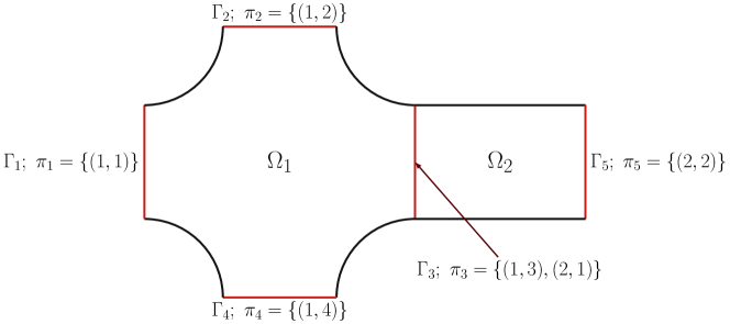
Figure 1: Illustration of PRSC nomenclature in a two-component system; red segments of the boundary are ports, with their global index and index set shown.

The restriction of $X$ to $\gamma_{{i},{j}}$ (its “port space”) is denoted $P_{i,j}$. Where a global port $\Gamma_{p}$ is the coincidence of two local ports, $\pi_{p}=\left\{(i,j),(i^{\prime},j^{\prime})\right\}$, their port spaces are identical: $P_{i,j}=P_{{i^{\prime}},{j^{\prime}}}$. Letting the dimension of $P_{i,j}$ be $n^{\gamma}_{i,j}$, define a basis $\left\{\chi_{i,j,k}\in P_{i,j},\ k\in\left\{1,\ldots,n^{\gamma}_{i,j}\right\}\right\}$ for $P_{i,j}$, and a “lifted port basis” $\left\{\psi_{i,j,k}\in X|_{\Omega_{i}},\ k\in\left\{1,\ldots,n^{\gamma}_{i,j}\right\}\right\}$, where $\psi_{i,j,k}|_{\gamma_{{i},{j}}}=\chi_{i,j,k}$ and $\psi_{i,j,k}|_{\gamma_{{i},{j^{\prime}}}}=0,\ j^{\prime}\neq j$. We lift the port bases by solving

$$\begin{split}a_{i}\left(\psi_{i,j,k},v;\boldsymbol{\mu}_{i;0}\right)&=0,\ \forall v\in B_{i}\\ \psi_{i,j,k}&=\chi_{i,j,k}\text{ on }\gamma_{{i},{j}}\\ \psi_{i,j,k}&=0\text{ on }\gamma_{{i},{j^{\prime}}},\ j^{\prime}\neq j.\end{split}$$ (4)

The global lifted port basis associated to $\Gamma_{p}$ is given by $\Psi_{{p},k}=\psi_{i,j,k}+\psi_{{i^{\prime}},{j^{\prime}},k}$ if $\pi_{p}=\left\{(i,j),(i^{\prime},j^{\prime})\right\}$, or $\Psi_{{p},k}=\psi_{i,j,k}$ if $\pi_{p}=\left\{(i,j)\right\}$, where port basis functions are extended by zero outside of their domain.

In addition to port spaces, each component has a “bubble space” defined as

$$B_{i}\equiv\left\{v\in X_{i}:v|_{\gamma_{{i},{j}}}=0,\ j\in\left\{1,\ldots,n_{i}^{\gamma}\right\}\right\}.$$ (5)

Define two classes of parameter dependent “bubble functions” by solution of the equations

$$a_{i}\left(b_{i,j,k}\left(\boldsymbol{\mu}_{i}\right),v;\boldsymbol{\mu}_{i}\right)=-a_{i}\left(\psi_{i,j,k},v;\boldsymbol{\mu}_{i}\right),\ \forall v\in B_{i}$$ (6)

$$a_{i}\left(b^{f}_{i}\left(\boldsymbol{\mu}_{i}\right),v;\boldsymbol{\mu}_{i}\right)=f_{i}\left(v;\boldsymbol{\mu}_{i}\right),\ \forall v\in B_{i}$$ (7)

where $b_{i,j,k},b^{f}_{i}\in B_{i}$. With these definitions, the solution to (1) on $\Omega_{i}$ may be written as:

$$u(\boldsymbol{\mu})|_{\Omega_{i}}=b^{f}_{i}\left(\boldsymbol{\mu}_{i}\right)+\sum_{j=1}^{n_{i}^{\gamma}}\sum_{k=1}^{n^{\gamma}_{i,j}}\mathbb{U}_{{\mathcal{G}_{i}(j)},{k}}\left(\boldsymbol{\mu}\right)\left(b_{i,j,k}(\boldsymbol{\mu}_{i})+\psi_{i,j,k}\right)$$ (8)

with $\mathbb{U}_{{p},{k}}$ unknown coefficients.

Defining interface functions $\phi_{{i},{j},{k}}(\boldsymbol{\mu}_{i})$ by

$$\phi_{{i},{j},{k}}(\boldsymbol{\mu}_{i})\equiv\psi_{i,j,k}+b_{i,j,k}(\boldsymbol{\mu}_{i})$$ (9)

and global interface functions $\Phi_{{p},{k}}(\boldsymbol{\mu})$ by

$$\Phi_{{p},{k}}(\boldsymbol{\mu})\equiv\sum_{(i,j)\in\pi_{p}}\phi_{{i},{j},{k}}(\boldsymbol{\mu}_{i}),$$ (10)

the global solution to (1) may be written as

$$u(\boldsymbol{\mu})=\sum_{i=1}^{n_{c}}b^{f}_{i}\left(\boldsymbol{\mu}_{i}\right)+\sum_{p=1}^{n^{\Gamma}}\sum_{k=1}^{n^{\Gamma}_{p}}\mathbb{U}_{{p},{k}}\left(\boldsymbol{\mu}\right)\Phi_{{p},{k}}\left(\boldsymbol{\mu}\right).$$ (11)

Substituting (11) in (1) and restricting test functions to the space spanned by the interface functions leads to the condensed system of equations

$$\mathbb{K}(\boldsymbol{\mu})\mathbb{U}(\boldsymbol{\mu})=\mathbb{F}(\boldsymbol{\mu}),$$ (12)

where the entries of $\mathbb{K}$ and $\mathbb{F}$ are

$$\mathbb{K}_{(p,k),(p^{\prime},k^{\prime})}=a\left(\Phi_{{p},{k}}\left(\boldsymbol{\mu}\right),\Phi_{{p^{\prime}},{k^{\prime}}}\left(\boldsymbol{\mu}\right);\boldsymbol{\mu}\right)$$ (13)

and

$$\mathbb{F}_{(p,k)}=f\left(\Phi_{{p},{k}}\left(\boldsymbol{\mu}\right);\boldsymbol{\mu}\right)-\sum_{i=1}^{n_{c}}a\left(b^{f}_{i}(\boldsymbol{\mu}_{i}),\Phi_{{p},{k}}\left(\boldsymbol{\mu}\right);\boldsymbol{\mu}\right).$$ (14)

A pair $(p,k)$ identifies a single degree of freedom in the linear system (12): the coefficient of $\Phi_{{p},{k}}$ in (11). The Schur complement consists of local contributions from each component, analagous to element stiffness matrices in a FEM. These contributions are defined by

$$\mathbb{K}^{i}_{(j,k),(j^{\prime},k^{\prime})}=a_{i}\left(\phi_{{i},{j},{k}}(\boldsymbol{\mu}_{i}),\phi_{{i},{j^{\prime}},{k^{\prime}}}(\boldsymbol{\mu}_{i});\boldsymbol{\mu}_{i}\right).$$ (15)

We make use of this definition in sensitivity analysis.

In this description we have referred only to a collection of $n_{c}$ different subdomains $\Omega_{i}$ and termed these “components”. In practice a distinction is made between reference and instantiated components. Each instantiated component is associated to a corresponding reference component, where the number of reference components is small, but $n_{c}$ may be very large. An offline data set needs only to be constructed for the small number of reference components, and is used to construct the linear system (12) using efficient operations on the offline data set. To simplify the presentation of PRSC we have avoided introducing separate notation for instantiated and reference components and describing the correspondence between the two, but these details are key to the efficient implementation of the method.

This description of PRSC so far only includes static condensation. Model reduction is incorporated by using a reduced port basis

$$\left\{\tilde{\chi}_{i,j,k}\in P_{i,j},\ k\in\{1,\ldots,\tilde{n}^{\gamma}_{i,j}\}\right\},$$

with reduced port basis dimension $\tilde{n}^{\gamma}_{i,j}<n^{\gamma}_{i,j}$, and corresponding lifted port basis functions $\tilde{\psi}_{i,j,k}$. In presenting the Schur complement system, we have used the notation for the full order model; however, the reduced order system may be derived by substituting the reduced lifted port basis and its dimension wherever the full order lifted port basis and its dimension appear. Henceforth, ROM quantities are denoted by adding a tilde to their FOM counterpart; for example, $\tilde{u}$ is the ROM solution for displacement. We determine an appropriate reduced port basis using the pairwise training procedure described in [10, Algorithm 2] and proper orthogonal decomposition with respect to the $L^{2}$ inner product on each port.

3 A component-wise formulation for topology optimization with stress constraints

Here we present the main contribution of this work: a method for stress-based TO that leverages PRSC to enable an efficient optimization, even when using a high-resolution discretization. With the use of PRSC, we also inherit its greatest advantage, which is the ability to reuse the component library constructed in the offline phase to model any arrangement of instantiated components. This allows the use of the same offline dataset to solve many TO problems in various geometries.

Below, we describe our methodology in detail: the formulation of the optimization problem, the material model and parameterization, the form of the aggregated stress constraints, and finally, postprocessing considerations.

3.1 Optimization formulation

Our goal is to solve the problem

$$\underset{\boldsymbol{\rho}\in\{0,1\}^{n_{c}}}{\text{minimize}}\hskip 5.0pt\mathcal{J}(\boldsymbol{\rho})=\sum_{i=1}^{n_{c}}\rho_{i}\left|\Omega_{i}\right|$$ (16)

$$\text{s.t.}\max_{\Omega}\hskip 5.0pt\sigma(\boldsymbol{\rho})\leq\sigma_{max},$$

where $\boldsymbol{\rho}\in\{0,1\}^{n_{c}}$ is the parameter vector, containing a density for each component in the system with $\rho_{i}=0$ meaning that component $i$ is removed and $\rho_{i}=1$ meaning that component $i$ is fully solid; $\left|\Omega_{i}\right|$ is the volume of $\Omega_{i}$; $\mathcal{J}(\boldsymbol{\rho})$ gives the mass of the system; and $\sigma$ is some yield criterion. In this work, $\sigma$ is the Von Mises yield stress. $\sigma_{max}$ is an upper bound on the allowed value of the yield criterion $\sigma$.

To render (LABEL:eq:basic_formulation) solvable by a gradient-based optimization solver, we make two changes following common practice. The first is to allow the component densities to reside in a continuum: $\boldsymbol{\rho}\in[0,1]^{n_{c}}$. Material properties for intermediate densities are interpolated by a standard SIMP scheme. Second, because of the non-differentiable nature of the max function, we replace the constraint in (LABEL:eq:basic_formulation) with a differentiable approximation. With these modifications, the optimization formulation becomes:

$$\underset{\boldsymbol{\rho}\in[0,1]^{n_{c}}}{\text{minimize}}\hskip 5.0pt\mathcal{J}(\boldsymbol{\rho})=\sum_{i=1}^{n_{c}}\rho_{i}\left|\Omega_{i}\right|$$ (17)

$$\text{s.t.}\ g_{m}(\boldsymbol{\rho})\leq 1,\ 1\leq m\leq n_{agg},$$

with the aggregate constraints $g_{m}$ defined in Section 3.3.2. This is the optimization formulation that we actually solve. A local minimum of (LABEL:eq:actual_formulation) provides an approximation to solution of (LABEL:eq:basic_formulation), but the challenging integer programming problem has been replaced by one solvable using gradient-based nonlinear optimization solvers.

3.2 Material model & component-based parameterization

We model a material described by isotropic linear elasticity. On each component, the bilinear form $a_{i}$ is given by

$$a_{i}(u,v;\rho_{i})=\int_{\Omega_{i}}s(\rho_{i})\mathbb{C}(u)\cdot\nabla v\ dx,$$ (18)

where $s$ is the SIMP penalization term and $\mathbb{C}$ is the symmetric elasticity tensor given by

$$\mathbb{C}(u)=\mu\left(\nabla u+\nabla u^{T}\right)+\lambda(\nabla\cdot u)\boldsymbol{I},$$ (19)

with $\lambda$ and $\mu$ the Lamé parameters. Note that $\mu$ is a fixed material parameter and bears no relation to the vector of component parameters $\boldsymbol{\mu}_{i}$ from the discussion of PRSC. In our optimization formulation $\boldsymbol{\mu}_{i}=\left[\rho_{i}\right]$, so we use the scalar parameter $\rho_{i}$ in its place. This form for $a_{i}$ satisfies the necessary assumptions to implement the affine simplification of PRSC described in our previous work [22]. This simplification allows us to compute Schur complement contributions offline, making the model even more economical than PRSC without this simplification.

The linear form $f_{i}$ is

$$f_{i}(v)=\int_{\Omega_{i}}F\cdot v\ dx,$$ (20)

where $F$ is the vector of forces applied per unit volume. We assume $F$ to be independent of parameter in this work; this assumption is not necessary, but simplifies the sensitivity analysis.

We aim to obtain a “black and white” solution, $\rho_{i}\in\left\{0,1\right\}$. To drive the continuous density values to black and white solutions, we use the solid isotropic material (SIMP) parameterization [3, 42]. The Young’s modulus is penalized using a power law in the density: $E_{i}\propto\rho_{i}^{p}$, with $E_{i}$ the Young’s modulus of the material in $\Omega_{i}$. In our optimizations, we choose $p=3$. To ensure a well-posed problem, the SIMP parameterization is modified so that $s(\rho_{i})$ in (18) is given by

$$s(\rho_{i})=\left[\rho_{i}+(1-\rho_{i})\rho_{min}\right]^{3},$$ (21)

where $\rho_{min}>0$ is chosen to be small ($10^{-3}$). This ensures that the linear system (12) possesses a solution, but the stiffness of components with $\rho_{i}=0$ is negligible compared to components with $\rho_{i}=1$.

This parameterization is the same as a typical topology optimization using element-wise density variables, but enables the use of a component-wise ROM to reduce the computational cost because each component ROM only depends on a single density parameter. In a conventional, element-based density TO, the large dimension of parameter space makes model reduction impractical. The component-wise scheme has an additional benefit: it obviates the need for a density filter (as in [20, 14, 28, 21] and others) to avoid checkerboarding. The imposition of a ground structure intrinsically imposes a length scale without the use of a filter.

3.3 Imposing stress constraints using the ROM

Our formulation of stress constraints consists in three parts: stress relaxation, aggregation using the KS functional, and rewriting of the aggregate constraints using ROM operators. Of these parts, the first two are standard practice; the rewriting using ROM operators is an original contribution.

3.3.1 Stress relaxation

It is well known that stress constraints in the absence of some relaxation result in an optimization problem where minima are contained in a degenerate subspace (the “singularity problem”) [18]. As remarked in [9], this occurs where material in some region must vanish to reach a local optimum, but the material remains strained so that solutions for intermediate densities in that region violate constraints. When material has vanished, however, these constraints should be ignored – the constraint is discontinuous. Stress relaxation smooths this discontinuity to allow a gradient-based optimization algorithm to reach solutions in the degenerate subspace.

We adopt the $qp$-relaxation proposed by Bruggi [6], with the particular choice of $q=2.5$ as in [20, 14]. Denoting the Von Mises yield stress by $\sigma_{vm}$, the relaxed stress is then given by

$$\sigma_{r}|_{\Omega_{i}}=s^{\prime}(\rho_{i})\sigma_{vm},$$ (22)

where $\sigma_{vm}$ is the Von Mises stress as computed using the stiffness of the base material (not the SIMP penalized stiffness), and

$$s^{\prime}(\rho_{i})=\rho_{i}^{1/2}.$$ (23)

We note that the optimization has the trivial solution $\boldsymbol{\rho}=\boldsymbol{0}$; in practice, this solution is not reached by the optimizer. Convergence to the trivial solution, if problematic, could be addressed by imposing a lower bound on $s^{\prime}(\rho_{i})$ in the same fashion as in (21). Applying stress relaxation, the stress constraint becomes

$$\max_{\Omega}\ \sigma_{r}(\boldsymbol{\rho})\leq\sigma_{max},$$ (24)

which is identical to the constraint in (LABEL:eq:basic_formulation) for black and white solutions.

3.3.2 Stress aggregation

We cannot use the constraint (24) in a gradient-based optimization because the max function is non-differentiable. To circumvent this difficulty, we use stress aggregation to provide a differentiable approximation of the max function. Aggregation strategies include the $p$-norm, the Kreisselmeier-Steinhauser (KS) functional, or an “induced aggregation” functional as described by Kennedy and Hicken [17]. We use a continuous KS aggregation, with stresses aggregated over multiple aggregation domains (as in [14, 20], and others). For numerical stability in finite precision arithmetic, we aggregate the ratio of the relaxed stress to the maximum stress, rather than the relaxed stress itself. The single constraint (24) becomes $n_{agg}$ constraints given by

$$g_{m}(\boldsymbol{\rho})=\frac{1}{p}\ln\left(\frac{1}{\alpha}\int_{\Omega^{agg}_{m}}\exp\left(p\frac{\sigma_{r}(\boldsymbol{\rho})}{\sigma_{max}}\right)dx\right)\leq 1,\ 1\leq m\leq n_{agg},$$ (25)

where $p$ and $\alpha$ are fixed parameters of the aggregation. Increasing $p$ results in a closer approximation of the max function, but also a more difficult optimization problem. $\alpha$ is a normalization, whose determination we address below. The aggregation domains $\Omega^{agg}_{m}$ are not the same as component domains $\Omega_{i}$, nor even spatially contiguous domains. Their determination is addressed in the next section. Ideal values of $p$ and $n_{agg}$ are problem dependent, and studied in our numerical experiments.

The normalization $\alpha$ is computed based on the following observation from [[]Eq. 8]kennedy_hicken_induced_2015: for given values of $\boldsymbol{\rho}$ and $p$, we will have

$$g_{m}(\boldsymbol{\rho})\geq\max_{\Omega^{agg}_{m}}\frac{\sigma_{r}(\boldsymbol{\rho})}{\sigma_{max}}$$

if

$$\alpha\leq\int_{\Omega^{agg}_{m}}\exp\left(\frac{p}{\sigma_{max}}\left[\sigma_{r}-\max_{\Omega^{agg}_{m}}\sigma_{r}\right]\right)dx.$$ (26)

Let the initial value of $\boldsymbol{\rho}$ in the optimization be $\boldsymbol{\rho}_{0}$. Using (26), we compute values of $\alpha$ for each aggregation domain at the initial condition of the optimization as follows: compute

$$\alpha_{k}=\exp\left(\frac{p}{\sigma_{max}}\left[\max_{\Omega^{agg}_{m}}\sigma_{r}(\boldsymbol{\rho}_{0})\right]\right)^{-1}\int_{\Omega^{agg}_{m}}\exp\left(\frac{p}{\sigma_{max}}\sigma_{r}(\boldsymbol{\rho}_{0})\right)dx,$$ (27)

then set $\alpha$ for all aggregates to be equal to the minimum of all $\alpha_{k}$.

3.3.3 Achieving a conservative optimization result

The aggregation described in the previous section is not necessarily conservative; for some values of $\boldsymbol{\rho}$, the constraints (25) may be satisfied while the true max stress constraint (24) is not. To consider an optimization successful, we require satisfaction of the latter. In most cases determining $\alpha$ from Eq. (27) is sufficient to obtain a conservative optimization solution; where this is not the case, we use a simple heuristic: substitute $\hat{\sigma}_{max}<\sigma_{max}$ for $\sigma_{max}$ in (25). The choice of $\hat{\sigma}_{max}$ is problem dependent. Values used are reported in the numerical experiments – for most, $\hat{\sigma}_{max}=\sigma_{max}$.

This heuristic approach has mathematical justification. Eq. (25) may be rewritten as

$$g_{m}(\boldsymbol{\rho})=\frac{1}{p}\ln\left[\int_{\Omega^{agg}_{m}}\exp\left(p\frac{\sigma_{r}(\boldsymbol{\rho})}{\sigma_{max}}\right)dx\right]-\frac{\ln\alpha}{p}-1\leq 0.$$ (28)

Thus if $\alpha<e$, the value of the constraint is increased by a constant factor. A decrease in the upper bound in the optimization likewise corresponds to a constant increase in the value of $g_{m}$; therefore the imposition of $\hat{\sigma}_{max}<\sigma_{max}$ may be viewed as a correction to the value of $\alpha$ estimated from (26), necessary because that value is conservative only for a particular value of $\boldsymbol{\rho}$.

We also assign aggregation regions differently from previous works. The two main strategies are to either distribute stress evenly among aggregation regions [20], or to assign the highest stresses to a single aggregation region, resulting in a better approximation of the maximum in that region [14]. However, because we do not adaptively reassign regions and cannot know how stresses will be distributed at a given optimization iteration, neither of these approaches is possible here. Instead, we approximate the effect of an approach that computes an even distribution of stresses by assigning aggregation regions randomly. For each $\Omega_{i}$, we randomly assign an equal number of elements to each of the $n_{agg}$ aggregation domains $\Omega^{agg}_{m}$ (illustrated in Fig. 2). Ideally, this assignment of aggregation regions results in a problem where stresses are evenly distributed between the different aggregation regions. We show results on the same problem for different assignments of aggregation regions in Section 4.3.2.

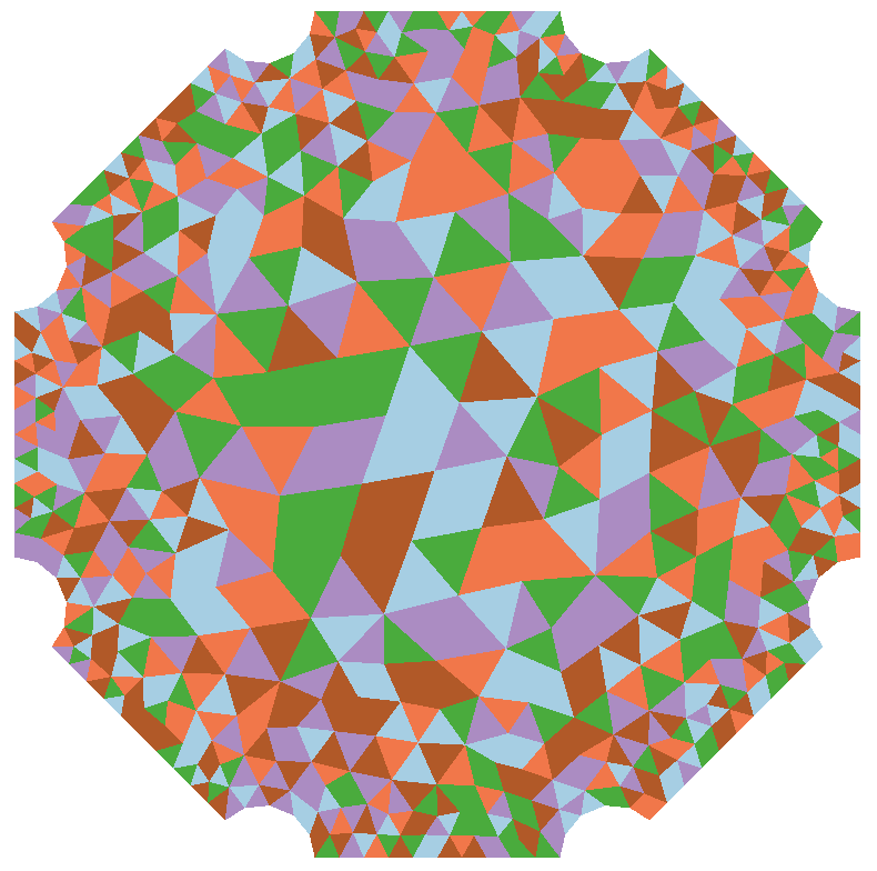
Figure 2: Illustration of aggregation region assignment for a single component and five aggregation regions. Elements contained in the same aggregation region are assigned the same color.

3.3.4 Efficient computation of aggregates using the CWROM

The aggregation in Eq. (25) is nonlinear in $\sigma_{vm}$, which is in turn a nonlinear function of displacement. This nonlinearity prohibits the expression of the constraints in terms of $\tilde{\mathbb{U}}(\boldsymbol{\rho})$ without reconstructing the displacement field $\tilde{u}(\boldsymbol{\rho})$. However, computing the constraints by reconstructing $\tilde{u}(\boldsymbol{\rho})$ and performing quadrature in a loop over elements is inefficient because of the high dimension of the underlying discretization. For example, in our smaller numerical example of Section 4.2, the mesh underlying the component-wise ROM has about 2.5 million elements. Integration over each element requires retrieving coefficients of the finite element basis functions, which are generally not contiguous in memory, and computing values of the non-linear integrand as a function of these coefficients. While it is not possible to remove the dependence of the cost of aggregation on the FOM dimension, we reduce the cost by expressing aggregation in terms of more cache-friendly operations using $\tilde{\mathbb{U}}(\boldsymbol{\rho})$ instead of $\tilde{u}(\boldsymbol{\rho})$.

We rewrite the constraints in terms of the ROM by noting that $\sigma_{vm}$, which is not linear in displacement, may be written as a function of the Cauchy stress tensor components. Limiting ourselves to two dimensions, we define vectors

$$\boldsymbol{\sigma}^{m}_{xx}\left(\tilde{\mathbb{U}}(\boldsymbol{\rho})\right)=S^{m}_{xx}\tilde{\mathbb{U}},\ \boldsymbol{\sigma}^{m}_{yy}\left(\tilde{\mathbb{U}}(\boldsymbol{\rho})\right)=S^{m}_{yy}\tilde{\mathbb{U}},\ \boldsymbol{\sigma}^{m}_{xy}\left(\tilde{\mathbb{U}}(\boldsymbol{\rho})\right)=S^{m}_{xy}\tilde{\mathbb{U}}$$ (29)

containing the values of stress tensor components at quadrature points for aggregation region $\Omega^{agg}_{m}$. We assume that there are no forces applied except on ports. Then, from the definition of the Cauchy stress tensor and Eq. (11), the linear operators $S^{m}_{xx}$, $S^{m}_{yy}$, and $S^{m}_{xy}$ are given by:

$$\begin{split}S^{m}_{xx}&=(2\mu+\lambda)\tilde{\Phi}^{m}_{x,x}+\lambda\tilde{\Phi}^{m}_{y,y}\\ S^{m}_{yy}&=(2\mu+\lambda)\tilde{\Phi}^{m}_{y,y}+\lambda\tilde{\Phi}^{m}_{x,x}\\ S^{m}_{xy}&=\mu\left(\tilde{\Phi}^{m}_{x,y}+\tilde{\Phi}^{m}_{y,x}\right),\end{split}$$ (30)

with $\tilde{\Phi}^{m}_{x,x}$ a matrix such that $\left[\tilde{\Phi}^{m}_{x,x}\right]_{j,k}$ contains the partial derivative with respect to $x$ of the $x$ component of the $k$-th interface function at the $j$-th quadrature point in $\Omega^{agg}_{m}$, and $\tilde{\Phi}^{m}_{y,y}$, $\tilde{\Phi}^{m}_{x,y}$, and $\tilde{\Phi}^{m}_{y,x}$ defined similarly.

In terms of the stress tensor component vectors (29), the vector of Von Mises stresses at quadrature points in $\Omega^{agg}_{m}$ is given by

$$\boldsymbol{\sigma}^{m}_{VM}\left(\tilde{\mathbb{U}}(\boldsymbol{\rho})\right)=\left({\boldsymbol{\sigma}^{m}_{xx}}\odot{\boldsymbol{\sigma}^{m}_{xx}}+{\boldsymbol{\sigma}^{m}_{yy}}\odot{\boldsymbol{\sigma}^{m}_{yy}}-{\boldsymbol{\sigma}^{m}_{xx}}\odot{\boldsymbol{\sigma}^{m}_{yy}}+3{\boldsymbol{\sigma}^{m}_{xy}}\odot{\boldsymbol{\sigma}^{m}_{xy}}\right)^{1/2},$$ (31)

where $\odot$ denotes the Hadamard product and the exponentiation is applied element-wise. We omit the functional dependence of $\boldsymbol{\sigma}^{m}_{xx}$, etc. on $\tilde{\mathbb{U}}(\boldsymbol{\rho})$ for brevity. The vector of relaxed stresses at quadrature points is then

$$\boldsymbol{\sigma}_{r}^{m}\left(\boldsymbol{\rho},\tilde{\mathbb{U}}(\boldsymbol{\rho})\right)={s^{\prime}\left(\boldsymbol{\rho}^{m}_{agg}\right)}\odot{\boldsymbol{\sigma}^{m}_{VM}},$$ (32)

where $\boldsymbol{\rho}^{m}_{agg}$ contains the value of the density parameter at each quadrature point and $s^{\prime}$ is the relaxed stress (23), applied elementwise.

Taking $\boldsymbol{w}$ to be a vector containing the coefficients for quadrature over $\Omega^{agg}_{m}$, we can rewrite the constraints in Eq. (25):

$$g_{m}\left(\boldsymbol{\rho},\tilde{\mathbb{U}}(\boldsymbol{\rho})\right)=\frac{1}{p}\ln\left(\frac{1}{\alpha}\boldsymbol{w}^{T}\left[\exp\left(\frac{p}{\sigma_{max}}\boldsymbol{\sigma}_{r}^{m}\left(\boldsymbol{\rho},\tilde{\mathbb{U}}(\boldsymbol{\rho})\right)\right)\right]\right)-1\leq 0,$$ (33)

with exponentiation interpreted elementwise.

Although this expression improves the performance of aggregation by rewriting it in a more cache-friendly manner, the size of the stress operators in Eq. (30) grows with the number of quadrature points and the dimension of the ROM, until at some point it is more efficient to compute the aggregates in the obvious fashion. In our numerical examples, we use a four-point quadrature rule exact for second-order polynomials. Also, because we assign aggregation regions randomly, the stress operators in (30) cannot be computed offline; instead they are computed once at the beginning of the optimization. The cost of this computation is insignificant relative to the total cost of optimization.

3.3.5 Sensitivity analysis of stress constraints

To derive the gradient of the constraint $g_{m}$ with respect to $\boldsymbol{\rho}$, we note that $g_{m}(\boldsymbol{\rho})$ depends both directly on $\boldsymbol{\rho}$ and implicitly through $\tilde{\mathbb{U}}(\boldsymbol{\rho})$, with the latter dependence defined by the forward model. Therefore, the gradient is given by a total derivative:

$$\nabla_{\boldsymbol{\rho}}\ g_{m}\left(\boldsymbol{\rho},\tilde{\mathbb{U}}(\boldsymbol{\rho})\right)=\frac{\partial g_{m}}{\partial\boldsymbol{\rho}}+\left(\frac{d\tilde{\mathbb{U}}}{d\boldsymbol{\rho}}\right)^{T}\frac{\partial g_{m}}{\partial\tilde{\mathbb{U}}},$$ (34)

where the notation $\frac{d\tilde{\mathbb{U}}}{d\boldsymbol{\rho}}$ indicates the Jacobian matrix with

$$\left[\frac{d\tilde{\mathbb{U}}}{d\boldsymbol{\rho}}\right]_{i,j}=\frac{\partial\tilde{\mathbb{U}}_{i}}{\partial\rho_{j}}.$$

The action of $\left(\frac{d\tilde{\mathbb{U}}}{d\boldsymbol{\rho}}\right)^{T}$ is computed using the adjoint method. From Eq. (12), we have

$$\frac{d\tilde{\mathbb{K}}}{d\boldsymbol{\rho}}\tilde{\mathbb{U}}+\tilde{\mathbb{K}}\frac{d\tilde{\mathbb{U}}}{d\boldsymbol{\rho}}=\frac{d\tilde{\mathbb{F}}}{d\boldsymbol{\rho}}.$$ (35)

In our problem settings the forcing is independent of parameter and the above yields

$$\frac{d\tilde{\mathbb{U}}}{d\boldsymbol{\rho}}=-\tilde{\mathbb{K}}^{-1}\left[\frac{d\tilde{\mathbb{K}}}{d\boldsymbol{\rho}}\tilde{\mathbb{U}}\right].$$ (36)

By substitution in Eq. (34), we obtain the gradient:

$$\nabla_{\boldsymbol{\rho}}\ g_{m}\left(\boldsymbol{\rho},\tilde{\mathbb{U}}(\boldsymbol{\rho})\right)=\frac{\partial g_{m}}{\partial\boldsymbol{\rho}}-\left[\frac{d\tilde{\mathbb{K}}}{d\boldsymbol{\rho}}\tilde{\mathbb{U}}\right]^{T}\boldsymbol{\lambda},$$ (37)

where, making use of the symmetry of $\tilde{\mathbb{K}}(\boldsymbol{\rho})$, $\boldsymbol{\lambda}$ is given by solution of the adjoint equation

$$\tilde{\mathbb{K}}(\boldsymbol{\rho})\boldsymbol{\lambda}(\boldsymbol{\rho})=\frac{\partial g_{m}}{\partial\tilde{\mathbb{U}}}(\boldsymbol{\rho}).$$ (38)

Note that $\frac{d\tilde{\mathbb{K}}}{d\boldsymbol{\rho}}$ is a third-order tensor; for this sensitivity analysis, its product with $\tilde{\mathbb{U}}$ is defined by:

$$\left[\frac{d\tilde{\mathbb{K}}}{d\boldsymbol{\rho}}\tilde{\mathbb{U}}\right]_{ij}=\sum_{k}\frac{d\tilde{\mathbb{K}}_{ik}}{d\rho_{j}}\tilde{\mathbb{U}}_{k}$$ (39)

To close Eq. (34), we require expressions for the partial derivatives of $g_{m}$. These are found using the chain rule:

$$\frac{\partial g_{m}}{\partial\boldsymbol{\rho}} =\left(\frac{\partial\boldsymbol{\sigma}_{r}^{m}}{\partial\boldsymbol{\rho}}\right)^{T}\frac{\partial g_{m}}{\partial\boldsymbol{\sigma}_{r}^{m}}$$ (40)

$$\frac{\partial g_{m}}{\partial\tilde{\mathbb{U}}} =\left(\frac{\partial\boldsymbol{\sigma}_{r}^{m}}{\partial\tilde{\mathbb{U}}}\right)^{T}\frac{\partial g_{m}}{\partial\boldsymbol{\sigma}_{r}^{m}}.$$ (41)

Defining the vector

$$\boldsymbol{e}\left(\rho_{i},\tilde{\mathbb{U}}(\boldsymbol{\rho})\right)=\exp\left[\frac{p}{\sigma_{max}}\boldsymbol{\sigma}_{r}^{m}\left(\rho_{i},\tilde{\mathbb{U}}(\boldsymbol{\rho})\right)\right],$$ (42)

we find from Eq. (33) that $\frac{\partial g_{m}}{\partial\boldsymbol{\sigma}_{r}^{m}}$ is

$$\frac{\partial g_{m}}{\partial\boldsymbol{\sigma}_{r}^{m}}=\frac{1}{\sigma_{max}\ \boldsymbol{w}^{T}\boldsymbol{e}\left(\boldsymbol{\rho},\tilde{\mathbb{U}}(\boldsymbol{\rho})\right)}\ {\boldsymbol{e}\left(\boldsymbol{\rho},\tilde{\mathbb{U}}(\boldsymbol{\rho})\right)}\odot{\boldsymbol{w}}.$$ (43)

Finally, we require the derivatives of $\boldsymbol{\sigma}_{r}^{m}$ in Eqs. (40) and (41). With respect to $\boldsymbol{\rho}$, obtain

$$\frac{\partial\boldsymbol{\sigma}_{r}^{m}}{\partial\boldsymbol{\rho}}=P_{m}\left({\frac{ds^{\prime}}{d\rho}(\boldsymbol{\rho}^{m}_{agg})}\odot{\boldsymbol{\sigma}^{m}_{VM}}\right)\otimes I,$$ (44)

with $P_{m}$ a prolongation operator taking values in $\boldsymbol{\rho}^{m}_{agg}$ to their corresponding entry in $\boldsymbol{\rho}$ and padding with zeros for entries in $\boldsymbol{\rho}$ not corresponding to elements in $\Omega^{agg}_{m}$, and $\otimes$ denoting a row-wise Kronecker product.

With respect to $\tilde{\mathbb{U}}$, the Jacobian of $\boldsymbol{\sigma}_{r}^{m}$ is given by

$$\frac{\partial\boldsymbol{\sigma}_{r}^{m}}{\partial\tilde{\mathbb{U}}}=s^{\prime}\left(\boldsymbol{\rho}^{m}_{agg}\right)\otimes\frac{\partial\boldsymbol{\sigma}^{m}_{VM}}{\partial\tilde{\mathbb{U}}},$$ (45)

with $\frac{\partial\boldsymbol{\sigma}^{m}_{VM}}{\partial\tilde{\mathbb{U}}}$ given by

$$\frac{\partial\boldsymbol{\sigma}^{m}_{VM}}{\partial\tilde{\mathbb{U}}}=\frac{1}{2}\left(\boldsymbol{\sigma}^{m}_{VM}\right)^{-1}\otimes\left[2\boldsymbol{\sigma}^{m}_{xx}\otimes S^{m}_{xx}+2\boldsymbol{\sigma}^{m}_{yy}\otimes S^{m}_{yy}-\boldsymbol{\sigma}^{m}_{xx}\otimes S^{m}_{yy}-\boldsymbol{\sigma}^{m}_{yy}\otimes S^{m}_{xx}+6\boldsymbol{\sigma}^{m}_{xy}\otimes S^{m}_{xy}\right].$$ (46)

3.4 Postprocessing

SIMP penalization does not necessarily succeed at creating black and white solutions. Therefore, we postprocess by removing components with $\rho_{i}$ less than a prescribed minimum value $\rho_{min}$ from the domain entirely, and setting the densities of remaining components to unity. This reveals some amount of wasted mass in the structure where a component that was previously attached to another now has a “hanging” port not on a load-bearing path. In a post-processing step, we substitute streamlined versions of these components from a library of alternatives, as illustrated by Fig. 3. This procedure decreases the mass of the system from that at the local optimum, often substantially, and its implementation is simple in the component-wise framework.

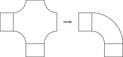
Figure 3: Illustration of replacing a component with two hanging ports by an alternative, streamlined geometry

4 Numerical results

We present numerical results for a pair of two-dimensional stress constrained problems. In the first, we minimize mass of an L-shaped bracket subject to a vertical load on its top right tip; in the second, we minimize the mass of a cantilever beam, also with a vertical load at the top right. The examples share the same material properties: Young’s modulus of 113.8 GPa, Poisson’s ratio of 0.34, and a Von Mises yield criterion of $\sigma_{max}=880$ MPa. Linear elasticity is approximated in two dimensions assuming plane stress conditions. We demonstrate that our methodology succeeds in creating designs that respect a constraint on maximum stress while approximating that constraint using PRSC and stress aggregation.

4.1 Problem setup

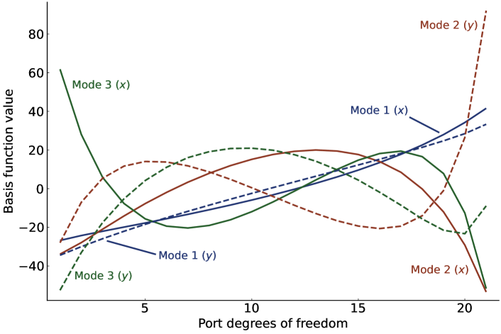
Figure 4: An example port basis, not including the constant function. The basis functions for the $x$ component of displacement are shown using a solid line; for the $y$ component, a dashed line.

The reduced order model used for our primary optimization results is trained by collecting 500 snapshots for each pair of connected reference ports and constructing port bases that capture 99.9% of the total energy of each snapshot set, unless a different total energy percentage is specified. When training, we compute the POD for the X and Y components of displacement separately but using the same snapshot set, and apply the total energy criterion to the POD for each component of displacement separately to determine bases. The regularization parameter for pairwise training was set to $\eta=10$ [10, Sec. 3.2.2]. The resulting bases contain four basis functions, including the constant function, for each component of displacement. An example reduced basis is pictured in Fig. 4. For our primary optimization results, the ROM is constructed using second-order triangular finite elements; the full basis for a port contains twenty-one basis functions for each component of displacement. We address the impact of using second-order elements vs. first-order in Section 4.2.3.

All optimizations are initialized from a fully solid ground structure, i.e., $\boldsymbol{\rho}=\boldsymbol{1}$. When postprocessing, we validate the optimized design by performing analysis with the full-order model. Maximum stress values in postprocessing are computed using values at cell centers, and at the quadrature points of a nine-point quadrature rule in each element. We do not consider values of stress on the boundary of an element due to its discontinuity there.

The optimization problem is solved using an interior point method as implemented in Ipopt [32]. We found it was necessary to set the parameter theta_max_fact to a small value (0.5 was used in these results) to prevent large steps into infeasible regions from which it is difficult for the optimizer to escape. For the same reason, we disable the watchdog procedure that attempts to escape regions of slow convergence by disabling line search for one iteration. In all of the optimization runs presented, Ipopt’s convergence tolerance was set to $10^{-6}$.

The Schur complement system is solved using a Cholesky factorization as implemented in Eigen [12], and all optimizations are performed without use of parallelism, for reproducibility. Timings are performed on a Linux server with 2 AMD EPYC 7H12 processors with 64 physical cores and a base clock speed of 2.6 GHz, and 2 TB of memory.

4.2 Mass minimization of an L-bracket

Our first example addresses the design of an L-shaped bracket, a standard benchmark in stress-based TO. While in most TO approaches the L-bracket presents a challenge because of its reentrant corner, using the component-wise methodology, we eliminate this difficulty by a careful choice of the ground structure.

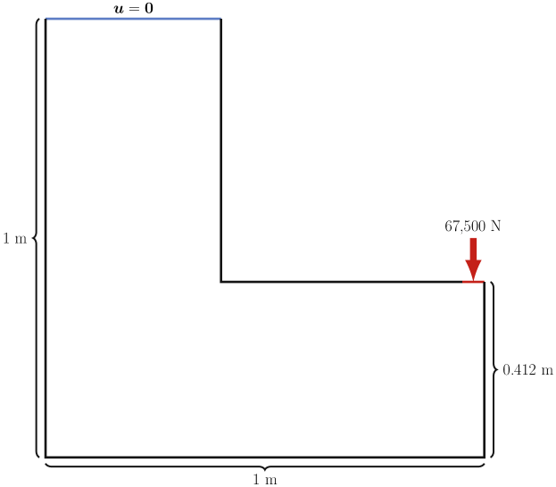
Figure 5: Illustration of the L-bracket geometry and loading condition.

The problem setup for the L-bracket optimization is illustrated in Figure 5. The thickness of the bracket into the page is taken to be 5 cm. The ground structure contains 4,257 components and 2,427,362 finite elements; the reduced static condensation system contains 44,214 unknowns while the full order static condensation system has 278,544. The underlying finite element model contains more than 5 million unknowns (not accounting for those degrees of freedom on ports, which are counted twice). The bracket’s upper boundary is fixed, and a load of 67,500 N is applied as an evenly distributed pressure force over the rightmost two ports at the tip of the bracket.

4.2.1 Optimization results and comparison of aggregation parameters

$n_{agg}$	$p$	$N_{cons}$	$N_{jac}$	Run time (s)	$m_{frac}^{opt}$	$m_{frac}^{pp}$	$\max\sigma_{r}$ (MPa)	$\max\sigma_{vm}$ (MPa)
1	10	5114	1985	9040	11.2%	8.7%	1215	938
5	10	716	394	1612	14.1%	14.1%	1148	889
10	10	903	524	2345	13.0%	11.5%	1217	888
15	10	649	328	1793	13.6%	13.5%	1229	884
20	10	877	457	2574	13.7%	13.3%	1215	886
25	10	1429	675	4255	13.3%	12.2%	1238	886
1	15	4531	1495	8188	15.5%	13.9%	892	907
5	15	3348	1498	6916	15.6%	13.8%	988	771
10	15	1117	536	2661	15.7%	13.7%	949	799
15	15	1113	502	2832	15.5%	13.6%	929	906
20	15	1362	580	3672	15.3%	12.2%	923	1074
25	15	1046	421	2935	14.8%	11.9%	957	695
1	25	6728	2287	12580	16.4%	13.0%	747	913
5	25	1984	1097	4504	17.6%	14.4%	735	704
10	25	1162	534	2835	17.9%	14.8%	725	698
15	25	1526	603	3960	18.5%	14.6%	707	731
20	25	1350	574	3768	18.0%	15.2%	714	686
25	25	1377	677	4167	19.5%	15.4%	725	765
1	50	-	-	-	-	-	-	-
5	50	4228	1906	8503	19.7%	17.3%	652	651
10	50	2466	1070	5701	21.2%	17.1%	610	602
15	50	2887	1233	7161	21.8%	16.5%	579	617
20	50	1984	826	5442	22.1%	17.8%	557	606
25	50	2489	1068	7116	22.8%	18.0%	560	592

Table 1: Summary of optimization results for varying aggregation parameters. For each combination of $n_{agg}$ and $p$, reported are, from left to right: number of constraint evaluations, number of constraint Jacobian evaluations, total run time, mass fraction at the local optimum, mass fraction after postprocessing, maximum relaxed stress at the optimum, and maximum Von Mises stress after postprocessing. Stresses are computed using the full order model in a postprocessing step.

We solve the optimization (LABEL:eq:actual_formulation) for values of the aggregation multiplier $p=$ 10, 15, 25, and 50, and with 1, 5, 10, 15, 20, and 25 aggregation regions. The results are summarized in Table 1, which records the number of constraint evaluations ($N_{cons}$), constraint Jacobian evaluations ($N_{jac}$), total optimization time, the mass fraction at convergence ($m_{frac}^{opt}$), the mass fraction after postprocessing ($m_{frac}^{pp}$), the maximum relaxed stress at convergence ($\max\sigma_{r}$), and maximum Von Mises stress in the postprocessed design ($\max\sigma_{vm}$). An optimization not terminating within 10,000 iterations is considered non-convergent, as in the case of the run for $p=50$ and $n_{agg}=1$. For all cases, the maximum stress for the optimization algorithm is not reduced from the desired maximum: $\hat{\sigma}_{max}=\sigma_{max}$. All designs are postprocessed using a dropping tolerance of $\rho_{min}=0.2$.

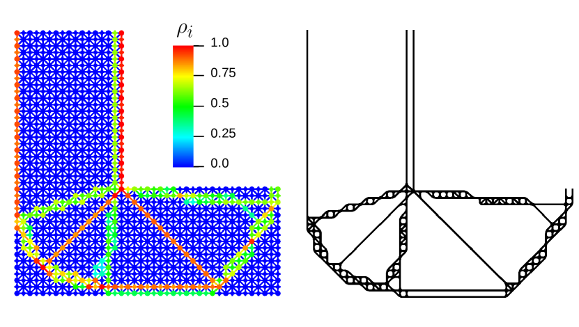
Figure 6: Optimization result using 10 aggregation regions and $p=15$. Left: locally optimal density field. Right: the resulting design after postprocessing. Maximum Von Mises stress in the postprocessed design is 799 MPa, compared to $\sigma_{max}=880$ MPa. Before postprocessing, the maximum relaxed stress was $\sigma_{r}=949$ MPa.

Fig. 6 illustrates the result using 10 aggregation regions and $p=15$, a representative optimization result. Many components at the local optimum have intermediate values of density; however, component densities are clearly divided between material and void components with densities being either greater than approximately $\rho=0.25$, or close to 0. This motivates our choice of dropping tolerance. Postprocessing creates a fully solid design that satisfies the desired stress constraint, as well as reducing the mass from the value at the local optimum, since many components are replaced with lighter substitutes despite having their density increased to 1 from an intermediate value. The design uses square lattice cells both with and without diagonal reinforcement in different areas of the design, as well as long, solid struts and larger open cells. We highlight here the flexibility of the component-wise approach over a design method that assumes a functionally graded structure, with regions composed of periodic unit cells.

Although we observe variability in the optimization’s performance, there are some general trends. First, increasing the aggregation multiplier $p$ results in the expected behavior: designs are more conservative, and the optimization problem is more difficult. Increasing the number of aggregation regions, however, does not have a discernable effect on the value of the maximum stress attained in the final design, at least for a moderate number of aggregation regions as used here. It does appear that adding regions is beneficial for convergence of the algorithm up to 10-15 regions; for values of $p=$ 15, 25, and 50, the number of constraint evaluations is reduced enough that overall run time is faster for ten aggregation regions than five, despite requiring twice the number of adjoint solves for each Jacobian evaluation.

In every case, the postprocessing step results in a mass that is less than or equal to to the objective value at the local optimum. In a few runs, however, it does result in violating the stress constraint because the nonlinear optimization cannot account for the changes made to the shape of components. Removing components with a near-zero density has a negligible effect on the structural response, but the component substitution step may have a large effect. In the examples using one aggregation region and $p=$ 15 and 25, we observe that component substitution results in increasing the maximum stress to a level that violates the max constraint, where before substitution it satisfied or nearly satisfied the constraint. In the example using 20 aggregation regions and $p=$ 15, a large increase in maximum stress is observed; however, this is due to the choice of $\rho_{min}=0.2$, which is too aggressive for this case and removes some components that have a smaller density but are structurally important. For other examples, the postprocessing step either results in a maximum stress that is less than the maximum relaxed stress at the local optimum, or increases it by a small amount such that the max constraint is still respected.

Despite variation across runs, it is clear that with a large enough choice of aggregation multiplier the proposed methodology consistently converges to conservative designs with a large mass reduction.

4.2.2 Performance of the ROM

We compare the accuracy of the ROM used for the primary results to results using a ROM trained with a 99.99% criterion for total energy as well as one using 99% of total energy. We define the following error measures:

$$e^{\sigma_{r}}_{max}=\frac{\max_{\Omega}\tilde{\sigma}_{r}-\max_{\Omega}\sigma_{r}}{\max_{\Omega}\sigma_{r}}$$ (47)

$$e^{\sigma_{r}}=\frac{\left\|\tilde{\sigma}_{r}-\sigma_{r}\right\|_{L^{2}}}{\left\|\sigma_{r}\right\|_{L^{2}}}$$ (48)

$$e^{u}=\frac{\left\|\tilde{u}-u\right\|_{L^{2}}}{\left\|u\right\|_{L^{2}}},$$ (49)

where $\tilde{\sigma}_{r}$ is the relaxed Von Mises stress as computed from the ROM solution, $\sigma_{r}$ is the relaxed Von Mises stress computed from the full-order solution, $\tilde{u}$ is the ROM displacement, and $u$ is the full-order displacement. The $L^{2}$ norm has its usual definition.

Reported in Table 2 are these errors for both the full system at the locally optimum parameter value, and for the postprocessed design. We report results for the designs using an aggregation multiplier of 15; the errors reported for these designs are representative of those for all designs. The exception is error of 13% in the postprocessed design for 5 aggregation regions, which is an outlier. In no other case was the error in maximum stress larger than 10%. The use of a 99.99% total energy criterion is sufficient to reduce the error in maximum stress to less than 5% in every case, and less than 1% for all but one; the effect on the displacement error is smaller. Errors when using a ROM capturing only 99% of total energy are large in every case; this criterion is clearly not strict enough to be useful.

	Errors at local optimum			Errors in postprocessed design
$n_{agg}$	$e^{\sigma_{r}}_{max}$	$e^{\sigma_{r}}$	$e^{u}$	$e^{\sigma_{r}}_{max}$	$e^{\sigma_{r}}$	$e^{u}$
Errors using 99.9% of total energy
1	-0.52%	4.12%	2.80%	-0.67%	2.96%	0.63%
5	3.17%	4.46%	4.18%	13.06%	2.93%	4.21%
10	-0.58%	3.67%	2.98%	-0.78%	2.84%	5.21%
15	6.42%	3.91%	4.04%	-0.98%	2.80%	1.96%
20	0.05%	4.17%	3.19%	0.09%	3.22%	3.35%
25	2.33%	3.78%	3.41%	8.66%	2.54%	4.44%
Errors using 99.99% of total energy
1	0.54%	2.72%	1.83%	0.02%	2.30%	0.49%
5	0.08%	3.05%	2.83%	-0.90%	2.28%	4.09%
10	0.02%	2.33%	2.01%	0.09%	2.33%	5.04%
15	4.03%	2.62%	2.68%	-0.08%	2.26%	1.94%
20	-0.79%	2.77%	2.11%	-0.18%	2.71%	3.24%
25	-0.98%	2.50%	2.27%	0.24%	2.10%	4.34%
Errors using 99% of total energy
1	155.67%	48.38%	25.88%	108.61%	21.24%	8.65%
5	167.64%	42.61%	29.99%	134.32%	21.10%	47.11%
10	160.05%	33.56%	21.75%	149.29%	19.87%	55.57%
15	173.93%	37.32%	30.97%	112.66%	20.84%	23.10%
20	176.95%	43.40%	23.86%	71.62%	19.09%	38.91%
25	140.72%	37.28%	25.13%	197.87%	17.45%	46.89%

Table 2: Comparison of ROM accuracies for different total energy criteria. Reported are relative errors in the maximum stress and relative errors in stress and displacement as measured in the $L^{2}$ norm for both the optimal parameter value and the postprocessed design.

Table 3 additionally reports the resulting number of degrees of freedom and the speedup relative to the full-order static condensation model for each total energy criterion. We report the speedup for the forward solve, which includes the cost of factoring the Schur complement matrix and is the largest component of optimization run time, and the speedup from use of our efficient aggregation scheme relative to the straightforward method using quadrature. Speedup is measured for the full system as used during the optimization procedure. The 99.9% total energy model achieves a speedup of more than a two orders of magnitude vs. a full-order static condensation solve, and the efficient aggregation scheme yields an almost 2.5x speedup vs. straightforward quadrature. In [22], we found that the full-order static condensation achieved approximately a 5x speedup compared to the underlying finite element model; thus, we estimate that the 99.9% total energy ROM used in these optimizations will provide approximately a 750x speedup over a finite element solve using the same mesh.

Criterion	Total DOFs	Forward speedup	Aggregate speedup
99%	44,214	224x	2.78x
99.9%	53,056	151x	2.47x
99.99%	70,740	59.6x	1.54x

Table 3: ROM speedups vs. a full-order static condensation solve for the forward solve, and a straightforward quadrature for the computation of stress aggregates.

4.2.3 Comparison to results using first-order elements

We also inquire whether the use of second-order finite elements to construct the ROM is actually beneficial. We expect that the resulting stresses in element interiors are more accurate, but it is uncertain whether this increased accuracy has a beneficial effect in the optimization. To determine whether it does, we ran optimizations using a ROM constructed using first-order elements and a 99.9% total energy criterion to compare to the corresponding results using second-order elements. These optimizations use $p=15$ and 10, 15, 20 and 25 aggregation regions, respectively. The ROM constructed using first-order elements has exactly the same dimension as that constructed using second-order elements, and the quadrature rule used to compute stress aggregates is identical. The aggregation regions are also identical to those used for the optimizations in Section 4.2.1.

			1st-order elements		2nd-order elements
$n_{agg}$	Run time (s)	$m_{frac}^{pp}$	$\max\sigma_{r}$	$\max\sigma_{vm}$	$\max\sigma_{r}$	$\max\sigma_{vm}$
10	13936	10.6%	1063	769	1215	944
15	3287	13.5%	1020	962	1195	1023
20	2743	11.8%	1001	899	1148	910
25	4699	11.1%	1026	1027	1153	1155

Table 4: Optimization results using a ROM constructed with first-order elements as the underlying model. We show the optimization run time and postprocessed mass fraction from an optimization run using first-order elements, and maximum stresses at the optimum and in the postprocessed design as computed using both first- and second-order elements. These stresses are computed using the corresponding full-order models.

To compare the optimization results we examine the run time, mass fraction of the postprocessed design, and the max stresses at the optimum and in the postprocessed design. The latter are computed using both the full-order first-order finite element model and the full-order second-order finite element model to assess the impact of second-order elements on accuracy in the stress. The results are summarized in Table 4; the optimization run time and mass fraction may be compared to the second block in Table 1. We find that the first-order model underestimates the maximum stress significantly. As a result, the optimized mass fractions are smaller than the corresponding optimization results with second-order elements, but none of the designs found using first-order elements is conservative when analyzed using second-order elements. Additionally, in three out of four cases, the optimization with first-order elements as the model had a longer run time than the second-order optimization. This is due to the fact that the ROM constructed from first-order elements has the same dimension as that constructed with second-order elements, while the optimizer spent additional model evaluations on line search in these cases. These results justify the use of the second-order model for our primary results.

4.2.4 Effect of decreasing the maximum stress

To verify that the heuristic of imposing a reduced stress limit $\hat{\sigma}_{max}$ (Sec. 3.3.3) achieves the desired effect, we solve the optimization problems with $p=10$ using $\hat{\sigma}_{max}=800$ MPa. The corresponding optimizations with $\hat{\sigma}_{max}=880$ MPa yielded postprocessed designs that did not satisfy the stress constraint. Results are reported in Table 5 in the same format as those in Table 1.

$n_{agg}$	$p$	$N_{cons}$	$N_{jac}$	Run time (s)	$m_{frac}^{opt}$	$m_{frac}^{pp}$	$\max\sigma_{r}$ (MPa)	$\max\sigma_{vm}$ (MPa)
$\hat{\sigma}_{max}=800$ MPa
1	10	2399	1251	4572	15.2%	12.9%	1159	910
5	10	827	517	1866	16.2%	14.9%	996	775
10	10	803	458	2047	16.2%	14.8%	984	698
15	10	702	384	1887	16.3%	15.4%	1029	704
20	10	806	484	2393	15.5%	13.6%	994	885
25	10	979	564	3009	16.0%	14.1%	970	906
$\hat{\sigma}_{max}=880$ MPa
1	10	5114	1985	9040	11.2%	8.7%	1215	938
5	10	716	394	1612	14.1%	14.1%	1148	889
10	10	903	524	2345	13.0%	11.5%	1217	888
15	10	649	328	1793	13.6%	13.5%	1229	884
20	10	877	457	2574	13.7%	13.3%	1215	886
25	10	1429	675	4255	13.3%	12.2%	1238	886

Table 5: Comparison of optimization results when decreasing the value of the stress limit for optimization. Consult Table 1 for definitions of the notation used here.

Setting $\hat{\sigma}_{max}<\sigma_{max}$ achieves a reduction in the maximum relaxed stress at the optimum in every case, as well as accelerating convergence in most cases. The effect after postprocessing is somewhat unpredictable. In the case with 25 aggregation regions, the maximum postprocessed stress using a lower upper bound for optimization is actually higher than that with the higher upper bound. In all other cases, the postprocessed stress was decreased. We expect that with enough reduction of $\hat{\sigma}_{max}$, optimization results will eventually lead to conservative postprocessed designs. Determining how much reduction is required, however, may require an iterative procedure and a choice that is too conservative will trade optimality for conservativeness. Instead, it may be preferable to choose a higher value for the aggregation multiplier $p$, and/or a larger number of aggregation regions. The choice of these parameters of the optimization is problem-dependent.

4.3 Mass minimization of a cantilever beam

Our second numerical example demonstrates how the component-wise approach solves a different structural optimization problem while using the same set of components. This illustrates a key advantage: the offline phase of constructing a component library need only be performed once, then the resulting dataset used to solve multiple design problems. We minimize the mass of a cantilever beam, fixed at one end and with a vertical load applied to the opposite tip. The problem setup is illustrated in Fig. 7; material properties are the same as for the L-bracket. The cantilever beam has a length of 1 m and height of approximately 25.8 cm (due to the lattice structure); a 30 kN load is applied to the rightmost two ports on the upper surface of the beam as an evenly distributed pressure force.

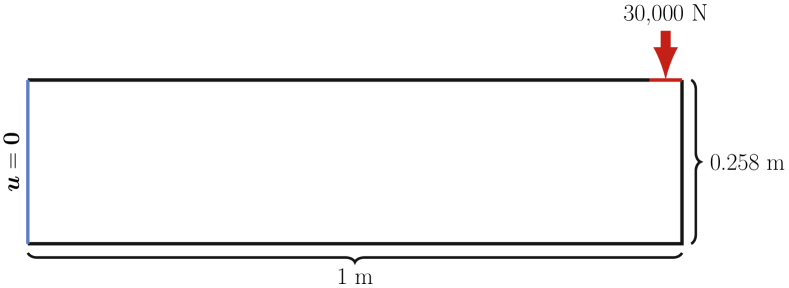
Figure 7: Setup for the cantilever beam optimization.

The underlying finite element mesh for the beam’s ground structure contains 3,750,278 second-order triangular elements for a total of more than 15 million degrees of freedom (not accounting for those duplicated on internal ports). The full-order static condensation system has 428,736 degrees of freedom, and the ROM constructed with 99.9% of total energy for port spaces contains 81,664.

4.3.1 Optimization result

We solve the optimization problem (LABEL:eq:actual_formulation) using 10 aggregation regions and an aggregation multiplier of $p=15$ and the ROM using a 99.9% total energy criterion. The convergence tolerance for Ipopt is set to $10^{-6}$. For this optimization, no reduction of the upper stress bound $\hat{\sigma}_{max}$ was necessary to obtain a conservative design. The optimization algorithm converges in 1,944 iterations with 2,576 constraint evaluations. At the local optimum, the mass fraction relative to the ground structure is 19.2%, with a maximum relaxed stress of $\sigma_{r}=849$ MPa. After postprocessing, the design has a mass fraction of 15.1% and maximum stress of 784 MPa. The result is postprocessed using dropping tolerance $\rho_{min}=0.25$.

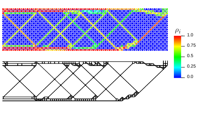
Figure 8: Results of the cantilever beam optimization. Top: optimized component-wise density field. Bottom: the postprocessed structure.

Fig. 8 shows the optimized density field and the result of postprocessing. As in the previous optimization results, many components have intermediate densities, but the chosen dropping tolerance clearly separates material and void regions. The postprocessed design resembles well-known results for compliance minimization problems and also has characteristics of functionally-graded structures – note the use of small repeating cells on the upper and lower boundaries, and a structure with a much larger void fraction in the interior.

4.3.2 Comparison to an optimization using different random aggregation regions

To justify the random assignment of aggregation regions, we compare optimization results for different choices of aggregation regions to the result shown previously. The postprocessed designs are compared to the previous one in Figure 9. The third result is postprocessed using a dropping tolerance of $\rho_{min}=0.2$ (vs. $\rho_{min}=0.25$ for the first two designs) because of component densities at the optimum that fall between these values but correspond to structurally important components.

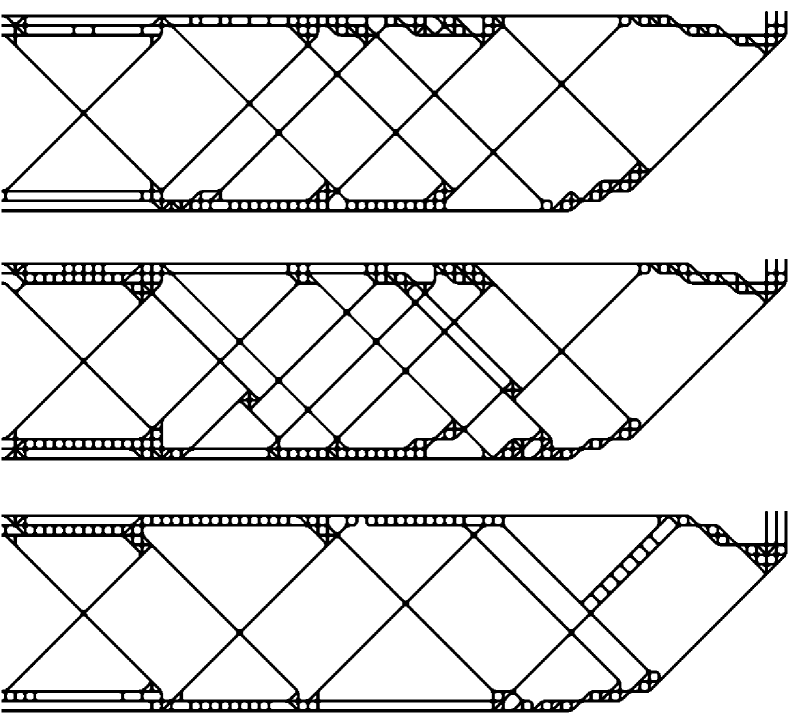
Figure 9: Comparison of the resulting postprocessed designs from three different random assignments of aggregation regions. Top: the design from Section 4.3.1, with a mass fraction of 15.1% and maximum stress of 784 MPa. Middle: the first design with redistributed aggregation regions, with mass fraction of 17.4% and a maximum stress of 806 MPa. Bottom: A third design with different aggregation regions, with mass fraction of 14.9% but a maximum stress of 1080 MPa.

Changing aggregation regions does make a significant difference in optimization results. Whereas the original optimization required 1,944 iterations to converge to tolerance, the optimizations with redistributed regions required only 793 and 1,428 respectively. We believe this is more indicative of the difficulty and sensitivity of the optimization problem than it is of a deficiency in the random strategy for region assignment. The local optima with new aggregation regions have mass fractions of 20.3% and 19%, vs. 19.2% in the original; after postprocessing, the mass fractions are 17.4% and 14.9% vs. the original 15.1%. Maximum relaxed stresses at the local optima are 849 MPa and 887 MPa, vs. the 860 MPa of the original design, and after postprocessing the new designs have maximum stresses of 806 MPa and 1080 MPa. Clearly the assignment of aggregation regions influences the quality of optimization results. We note, however, that the third design’s violation of the maximum stress constraint is due to postprocessing, not the assignment of aggregation regions; postprocessing creates a stress concentration that does not exist at the local optimum. Otherwise, random region assignments do result in fairly consistent designs.

5 Conclusions

We have presented a novel application of component-wise ROMs to stress constrained TO. The methodology succeeds in finding solutions with a large mass reduction relative to the ground structure while respecting stress constraints. While the presence of many local optima as well as the approximation of the maximum stress mean that it is impossible to guarantee a conservative solution, adjusting the aggregation multiplier and upper bound on stress proved effective for stress control. The reduced order model provides an error in the maximum stress of less than 10% in most cases and a relative error of about 3% in the $L^{2}$ norm, while providing a 150x speedup relative to a full order static condensation model. If greater accuracy is required, a ROM using 99.99% of total energy still provides a 60x speedup while reducing the error in the maximum stress by approximately an order of magnitude. Future work may investigate adaptive refinement of the ROMs to use the more accurate model only for components where it is needed, as permitted by the component-wise discretization. Due to the acceleration provided by the component-wise ROM, we are able to solve the TO problem efficiently on a ground structure containing millions of second-order finite elements. Component ROMs provide a high accuracy surrogate model that may be reused to study a multitude of both homogeneous and heterogeneous lattice-like structures.

Declaration of competing interest

The authors declare that they have no known competing financial interests or personal relationships that could have appeared to influence the work reported in this paper.

References

- [1] Jacob Aboudi “The Generalized Method of Cells and High-Fidelity Generalized Method of Cells Micromechanical Models—A Review” In Mechanics of Advanced Materials and Structures 11.4–5, 2004, pp. 329–366 DOI: 10.1080/15376490490451543
- [2] J. Ballani et al. “A component-based hybrid reduced basis/finite element method for solid mechanics with local nonlinearities” In Computer Methods in Applied Mechanics and Engineering 329, 2018, pp. 498–531 DOI: 10.1016/j.cma.2017.09.014
- [3] M.. Bendsøe “Optimal shape design as a material distribution problem” In Structural optimization 1.4, 1989, pp. 193–202 DOI: 10.1007/BF01650949
- [4] M.. Bendsøe and Noboru Kikuchi “Generating optimal topologies in structural design using a homogenization method” In Computer Methods in Applied Mechanics and Engineering 71.2, 1988, pp. 197–224 DOI: 10.1016/0045-7825(88)90086-2
- [5] M.. Bendsøe and Ole Sigmund “Material interpolation schemes in topology optimization” In Archive of Applied Mechanics 69.9, 1999, pp. 635–654 DOI: 10.1007/s004190050248
- [6] Matteo Bruggi “On an alternative approach to stress constraints relaxation in topology optimization” In Structural and Multidisciplinary Optimization 36.2, 2008, pp. 125–141 DOI: 10.1007/s00158-007-0203-6
- [7] Lin Cheng, Jiaxi Bai and Albert C. To “Functionally graded lattice structure topology optimization for the design of additive manufactured components with stress constraints” In Computer Methods in Applied Mechanics and Engineering 344, 2019, pp. 334–359 DOI: 10.1016/j.cma.2018.10.010
- [8] Hao Deng and Albert C. To “Linear and nonlinear topology optimization design with projection-based ground structure method (P-GSM)” In International Journal for Numerical Methods in Engineering 121.11, 2020, pp. 2437–2461 DOI: 10.1002/nme.6314
- [9] Pierre Duysinx and Ole Sigmund “New developments in handling stress constraints in optimal material distribution”, 7th AIAA/USAF/NASA/ISSMO Symposium on Multidisciplinary Analysis and Optimization, 1998 DOI: 10.2514/6.1998-4906
- [10] Jens L. Eftang and Anthony T. Patera “Port reduction in parametrized component static condensation: approximation and a posteriori error estimation” In International Journal for Numerical Methods in Engineering 96, 2013, pp. 269–302 DOI: 10.1002/nme.4543
- [11] Helen E. Fairclough, Matthew Gilbert and Andrew Tyas “Layout optimization of structures with distributed self-weight, lumped masses and frictional supports” In Structural and Multidisciplinary Optimization 65.2, 2022, pp. 65 DOI: 10.1007/s00158-021-03139-z
- [12] Gaël Guennebaud and Benoît Jacob “Eigen v3”, http://eigen.tuxfamily.org, 2010
- [13] Xu Guo, Weisheng Zhang and Wenliang Zhong “Doing Topology Optimization Explicitly and Geometrically—A New Moving Morphable Components Based Framework” In Journal of Applied Mechanics 81.8, 2014, pp. 081009 DOI: 10.1115/1.4027609
- [14] Erik Holmberg, Bo Torstenfelt and Anders Klarbring “Stress constrained topology optimization” In Structural and Multidisciplinary Optimization 48.1, 2013, pp. 33–47 DOI: 10.1007/s00158-012-0880-7
- [15] Laura Iapichino, Alfio Quarteroni and Gianluigi Rozza “Reduced basis method and domain decomposition for elliptic problems in networks and complex parametrized geometries” In Computers & Mathematics with Applications 71.1, 2016, pp. 408–430 DOI: 10.1016/j.camwa.2015.12.001
- [16] S. Kambampati, H. Chung and H.A. Kim “A discrete adjoint based level set topology optimization method for stress constraints” In Computer Methods in Applied Mechanics and Engineering 377, 2021, pp. 113563 DOI: https://doi.org/10.1016/j.cma.2020.113563
- [17] Graeme J. Kennedy and Jason E. Hicken “Improved constraint-aggregation methods” In Computer Methods in Applied Mechanics and Engineering 289, 2015, pp. 332–354 DOI: 10.1016/j.cma.2015.02.017
- [18] U. Kirsch “On singular topologies in optimum structural design” In Structural Optimization 2.3, 1990, pp. 133–142 DOI: 10.1007/BF01836562
- [19] Hyeong Seok Koh, Jun Hwan Kim and Gil Ho Yoon “Efficient topology optimization of multicomponent structure using substructuring-based model order reduction method” In Computers & Structures 228, 2020, pp. 106146 DOI: 10.1016/j.compstruc.2019.106146
- [20] Chau Le et al. “Stress-based topology optimization for continua” In Structural and Multidisciplinary Optimization 41.4, 2010, pp. 605–620 DOI: 10.1007/s00158-009-0440-y
- [21] Yangjun Luo and Zhan Kang “Topology optimization of continuum structures withDrucker–Prager yield stress constraints” In Computers & Structures 90–91, 2012, pp. 65–75 DOI: 10.1016/j.compstruc.2011.10.008
- [22] Sean McBane and Youngsoo Choi “Component-wise reduced order model lattice-type structure design” In Computer Methods in Applied Mechanics and Engineering 381, 2021, pp. 113813 DOI: https://doi.org/10.1016/j.cma.2021.113813
- [23] J.A. Norato, B.K. Bell and D.A. Tortorelli “A geometry projection method for continuum-based topology optimization with discrete elements” In Computer Methods in Applied Mechanics and Engineering 293, 2015, pp. 306–327 DOI: 10.1016/j.cma.2015.05.005
- [24] Max M.. Opgenoord and Karen E. Willcox “Design for additive manufacturing: cellular structures in early-stage aerospace design” In Structural and Multidisciplinary Optimization 60.2, 2019, pp. 411–428 DOI: 10.1007/s00158-019-02305-8
- [25] R. Picelli et al. “Stress-based shape and topology optimization with the level set method” In Computer Methods in Applied Mechanics and Engineering 329, 2018, pp. 1–23 DOI: https://doi.org/10.1016/j.cma.2017.09.001
- [26] Trenton M. Ricks et al. “Solution of the Nonlinear High-Fidelity Generalized Method of Cells Micromechanics Relations via Order-Reduction Techniques” In Mathematical Problems in Engineering 2018, 2018, pp. 1–11 DOI: 10.1155/2018/3081078
- [27] G… Rozvany “Difficulties in truss topology optimization with stress, local buckling and system stability constraints” In Structural optimization 11.3, 1996, pp. 213–217 DOI: 10.1007/BF01197036
- [28] Fernando V. Senhora, Oliver Giraldo-Londoño, Ivan F.. Menezes and Glaucio H. Paulino “Topology optimization with local stress constraints: a stress aggregation-free approach” In Structural and Multidisciplinary Optimization 62.4, 2020, pp. 1639–1668 DOI: 10.1007/s00158-020-02573-9
- [29] Ole Sigmund “Materials with prescribed constitutive parameters: An inverse homogenization problem” In International Journal of Solids and Structures 31.17, 1994, pp. 2313–2329 DOI: 10.1016/0020-7683(94)90154-6
- [30] Kathrin Smetana “A new certification framework for the port reduced static condensation reduced basis element method” In Computer Methods in Applied Mechanics and Engineering 283, 2015, pp. 352–383 DOI: 10.1016/j.cma.2014.09.020
- [31] Kathrin Smetana and Anthony T. Patera “Optimal Local Approximation Spaces for Component-Based Static Condensation Procedures” In SIAM Journal on Scientific Computing 38.5, 2016, pp. A3318–A3356 DOI: 10.1137/15M1009603
- [32] Andreas Wächter and Lorenz T. Biegler “On the implementation of an interior-point filter line-search algorithm for large-scale nonlinear programming” In Mathematical Programming 106.1, 2006, pp. 25–57 DOI: 10.1007/s10107-004-0559-y
- [33] Zijun Wu, Fei Fan, Renbin Xiao and Lianqing Yu “The substructuring-based topology optimization for maximizing the first eigenvalue of hierarchical lattice structure” In International Journal for Numerical Methods in Engineering 121.13, 2020, pp. 2964–2978 DOI: 10.1002/nme.6342
- [34] Zijun Wu, Liang Xia, Shuting Wang and Tielin Shi “Topology optimization of hierarchical lattice structures with substructuring” In Computer Methods in Applied Mechanics and Engineering 345, 2019, pp. 602–617 DOI: 10.1016/j.cma.2018.11.003
- [35] Liang Xia and Piotr Breitkopf “A reduced multiscale model for nonlinear structural topology optimization” In Computer Methods in Applied Mechanics and Engineering 280, 2014, pp. 117–134 DOI: 10.1016/j.cma.2014.07.024
- [36] Liang Xia and Piotr Breitkopf “Multiscale structural topology optimization with an approximate constitutive model for local material microstructure” In Computer Methods in Applied Mechanics and Engineering 286, 2015, pp. 147–167 DOI: 10.1016/j.cma.2014.12.018
- [37] Ran Xiao et al. “3D printing of titanium-coated gradient composite lattices for lightweight mandibular prosthesis” In Composites Part B: Engineering 193, 2020, pp. 108057 DOI: 10.1016/j.compositesb.2020.108057
- [38] Huikai Zhang, Yaguang Wang and Zhan Kang “Topology optimization for concurrent design of layer-wise graded lattice materials and structures” In International Journal of Engineering Science 138, 2019, pp. 26–49 DOI: 10.1016/j.ijengsci.2019.01.006
- [39] Shanglong Zhang, Arun L. Gain and J.A. Norato “Stress-based topology optimization with discrete geometric components” In Computer Methods in Applied Mechanics and Engineering 325, 2017, pp. 1–21 DOI: 10.1016/j.cma.2017.06.025
- [40] Weisheng Zhang et al. “A Moving Morphable Void (MMV)-based explicit approach for topology optimization considering stress constraints” In Computer Methods in Applied Mechanics and Engineering 334, 2018, pp. 381–413 DOI: 10.1016/j.cma.2018.01.050
- [41] Xiaojia Zhang, Adeildo S. Ramos and Glaucio H. Paulino “Material nonlinear topology optimization using the ground structure method with a discrete filtering scheme” In Structural and Multidisciplinary Optimization 55.6, 2017, pp. 2045–2072 DOI: 10.1007/s00158-016-1627-7
- [42] M. Zhou and G… Rozvany “The COC algorithm, Part II: Topological, geometrical and generalized shape optimization” In Computer Methods in Applied Mechanics and Engineering 89.1, Second World Congress on Computational Mechanics, 1991, pp. 309–336 DOI: 10.1016/0045-7825(91)90046-9