A CHEOPS Search for Massive, Long-Period Companions to the Warm Jupiter K2-139 b

Abstract

K2-139 b is a warm Jupiter with an orbital period of 28.4 d, but only three transits of this system have previously been observed, in the long-cadence mode of K2, limiting the precision with which the orbital period can be determined, and future transits predicted. We report photometric observations of four transits of K2-139 b with ESA’s CHaracterising ExOPlanet Satellite (CHEOPS), conducted with the goal of measuring the orbital obliquity via spot-crossing events. We jointly fit these CHEOPS data alongside the three previously-published transits from the K2 mission, considerably increasing the precision of the ephemeris of K2-139 b. The transit times for this system can now be predicted for the next decade with a $1\sigma$ precision less than 10 minutes, compared to over one hour previously, allowing the efficient scheduling of observations with Ariel. We detect no significant deviation from a linear ephemeris, allowing us to exclude the presence of a massive outer planet orbiting with a period less than 150 d, or a brown dwarf with a period less than one year. We also determine the scaled semi-major axis, the impact parameter, and the stellar limb-darkening with improved precision. This is driven by the shorter cadence of the CHEOPS observations compared to that of K2, and validates the sub-exposure technique used for analysing long-cadence photometry. Finally, we note that the stellar spot configuration has changed from the epoch of the K2 observations; unlike the K2 transits, we detect no evidence of spot-crossing events in the CHEOPS data.

1 Introduction

The atmospheres of many transiting exoplanets will be probed by Ariel, ESA’s M4 mission, which is due to launch in 2029 (Tinetti et al., 2018). Among the list of potential targets for Ariel is K2-139 b (Edwards et al., 2019). Maintaining accurate ephemerides of these targets is vital for the efficient operation of the mission. K2-139 b is one of the targets of interest of the ExoClock Project (Kokori et al., 2021, 2022), which aims to monitor the Ariel targets and improve their ephemerides, and is listed as a ‘high’ priority target as of 2022 March.

The issue of decaying ephemerides has also been studied recently from the point-of-view of NASA’s Transiting Exoplanet Survey Satellite (TESS; Ricker et al. 2015), which is expected to supply many of the bright targets for atmospheric characterization with Ariel and the James Webb Space Telescope (JWST; Gardner et al. 2006). Dragomir et al. (2020) found that if no further transits are observed, then around 80 per cent of the best exoplanetary targets for JWST (as selected by Kempton et al. 2018) would have transit timing uncertainties greater than 30 minutes by the time of the earliest possible JWST observations.

Many systems will be (re-)observed by TESS, which has completed its initial survey of the southern (Cycle 1) and northern (Cycle 2) skies, and is currently re-observing many of the Cycle 1 and 2 sectors. Klagyivik et al. (2021), for instance, recently updated the ephemerides of several transiting exoplanetary systems originally discovered by CoRoT (Moutou et al., 2013; Deleuil et al., 2018). However, according to the Web TESS Viewing Tool, no observations of K2-139 are planned within the first five years of TESS operations (up to and including Sector 69). Many systems can also be observed from the ground, with relatively small telescopes (e.g. Edwards et al. 2020, 2021a, 2021b), however longer-period systems such as K2-139 b are challenging targets for ground-based observations given their less frequent transits and longer transit durations.

K2-139 b was discovered during the re-purposed Kepler satellite’s K2 mission (Howell et al., 2014). Photometry from K2’s Campaign 7 revealed three transits of K2-139 b, and the system was subsequently observed and confirmed as a true planetary system by Barragán et al. (2018), hereafter ‘B18’. According to B18, K2-139 b is a warm Jupiter with a radius of $0.808\pm 0.034$ $\mathrm{R_{\rm Jup}}$ orbiting an active K0V star every 28.4 d. Radial velocity (RV) measurements of the star from the FIES, HARPS, and HARPS-N spectrographs allowed the mass of the planet to be determined as $0.387\begin{subarray}{c}+0.083\\ -0.075\end{subarray}$ $\mathrm{M_{\rm Jup}}$. The 1$\sigma$ uncertainty on the K2-139 b transit time predicted by the ephemeris of B18 reaches 30 minutes by early 2022, the time of the earliest JWST observations, and is well over an hour by the end of the decade, when Ariel may observe the system.

The spin-orbit angle or obliquity, i.e. the angle between the axis of stellar rotation and the orbital axis, of warm Jupiters is particularly interesting. Dynamical migration, whether through Kozai-Lidov cycles (Kozai, 1962; Lidov, 1962; Fabrycky & Tremaine, 2007) or planet – planet scattering (Rasio & Ford, 1996; Weidenschilling & Marzari, 1996) is expected to lead to planets on high-obliquity orbits. Warm Jupiters (unlike the closer-orbiting hot Jupiters) are not thought to experience strong-enough stellar tidal forces to later co-planarize their orbits. This means that the obliquities of warm Jupiters offer a unique insight into migration history.

While the obliquity has been measured for a significant sample of hot Jupiters, mostly via the Rossiter-McLaughlin effect, but also through Doppler tomographic observations, gravity-darkened transits, and by spot-crossing events, this is not the case for the warm Jupiters. According to TEPCat (Southworth, 2011), there are only nine obliquity measurements for warm Jupiters, compared to 120 for hot Jupiters. This is a result both of there being fewer known transiting warm Jupiters (49) than hot Jupiters (453), and of the difficulty, noted above, of observing the transits of longer-period planets from the ground.

Anomalies compatible with spot-crossing events were observed in all three transits observed by K2, and B18 note that this could be exploited to measure the obliquity of the system. This technique has been previously applied to the WASP-4 system (Sanchis-Ojeda et al., 2011) among others. Here, we present CHEOPS observations of K2-139 with the goal of constraining the obliquity, as well as updating the orbital ephemeris, of K2-139 b.

2 CHEOPS observations and data reduction

Table 1: Log of CHEOPS observations of K2-139

Visit no.	Start date	Duration	No. of	File_key	Efficiency†
	(UTC)	(h)	data points		(%)
1	2020 Jun 27 23:29	11.52	461	CH_PR210005_TG000101_V0200	69.4
2	2020 Jul 26 11:38	11.52	561	CH_PR210005_TG000201_V0200	64.2
3	2021 Jun 03 14:53	11.51	406	CH_PR210005_TG000202_V0200	71.7
4	2021 Jul 01 22:33	11.46	469	CH_PR210005_TG000203_V0200	66.6

^† The efficiency is the fraction of the visit spent collecting data.

Table 2: CHEOPS light curve of K2-139, produced by the CHEOPS DRP v13, using the OPTIMAL aperture radius. Only a sample is given here; the full table is available electronically from the CDS

$\mathrm{BJD_{TDB}}$	Flux	Flux	Spacecraft
- 2 450 000		uncertainty	roll angle ($\arcdeg$)
9028.503166	0.988975	0.000755	272.762
9028.503861	0.990507	0.000744	269.035
9028.504556	0.990557	0.000737	265.331

The CHaracterising ExOPlanet Satellite (CHEOPS; Benz et al. 2021) is a small (0.32-m diameter) telescope designed for high-precision monoband photometry of individual exoplanetary systems. CHEOPS was launched in 2019 December, and science operations commenced in 2020 April, with several studies (e.g. Lendl et al. 2020; Barros et al. 2022) already published reporting results from the mission. We observed four transits of K2-139 b with CHEOPS, under the Guest Observers’ (GO) programme AO-1-005 (PI: Smith).

The original aim was to observe four consecutive transits, to see if we could constrain the orbital obliquity of the system. Given the stellar rotation period of $17.24\pm 0.12$ d (B18), and the orbital period of 28.4 d, we would expect around 29 per cent of the stellar hemisphere visible during the first transit to be visible during the second transit, 41 per cent during the third, and 88 per cent during the fourth transit. We could therefore have expected to observe K2-139 b crossing the same spots in multiple transits if the obliquity is close to zero, and the spots have sufficient longevity, which B18 suggests they may.

Due to scheduling constraints, however, we in fact observed two consecutive transits in 2020 June and July, and a second pair of consecutive transits in 2021 June and July. Each ‘visit’ consisted of seven consecutive orbits of the CHEOPS satellite, or around 11.5 hours. With a $G$-band magnitude of 11.5, K2-139 is a relatively faint target for CHEOPS, and therefore an exposure time of 60 s was used. Further details of the observations are given in Table 1.

The data were reduced using the standard CHEOPS data reduction pipeline (DRP v13; Hoyer et al. 2020), which produces light curves using four different aperture radii: a ‘DEFAULT’ radius of 25 pixels, a slightly smaller ‘RINF’ radius of 22 pixels, a larger ‘RSUP’ radius of 30 pixels, and an ‘OPTIMAL’ radius. The size of the latter is determined on a per-visit basis, to account for the differing brightnesses of different targets, and is determined by minimising the noise-to-signal ratio (Hoyer et al., 2020). All four visits of K2-139 have the same optimized aperture radius of 15 pixels. We extracted each of these four light curves, corrected for the ‘ramp’ effect, using pycheops (Maxted et al., 2021). We tested each light curve, finding as expected that the light curves produced using the OPTIMAL radius give the highest signal-to-noise; this light curve is shown in Fig. 1, and in Table 2.

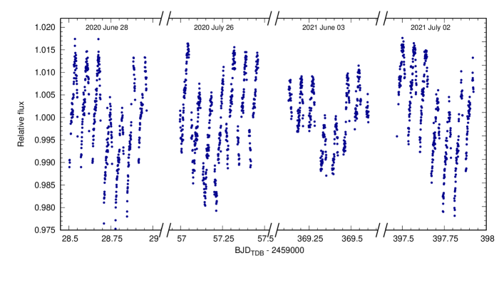
Figure 1: CHEOPS photometry of K2-139 produced by the DRP using the OPTIMAL aperture.

3 Stellar characterization

The previous characterization of K2-139 relied on a co-added FIES spectrum (B18). Here, we update the stellar characterization by fitting the spectral energy distribution (SED) of K2-139 using ariadne (Vines & Jenkins, 2022). The Phoenix v2 (Husser et al., 2013), BtSettl (Allard et al., 2012), Castelli & Kurucz (2003), and Kurucz (1993) stellar atmospheric model grids were fitted to catalog photometry (Table 7), constrained by the Gaia parallax. ariadne uses multiple model grids in order to account for the systematic errors arising from differences between different stellar atmosphere models. Gaussian priors from B18’s characterization were applied to $T_{\rm eff}$ and [Fe/H], and the distance was constrained using the Gaia DR2 parallax (Gaia Collaboration et al., 2018). Reddening was accounted for, with $A_{V}$ limited to the maximum line-of-sight value from the SFD Galactic dust map (Schlegel et al., 1998; Schlafly & Finkbeiner, 2011). Bayesian model averaging is employed by ariadne to derive the uncertainties from the posterior parameter distribution. The distributions for each model are averaged, weighted by the relative probability of each model, leading to smaller uncertainties than those obtained from any single model. ariadne has previously been used to characterize the primary star in several systems, both eclipsing binaries (Acton et al., 2020), and exoplanetary systems (Smith et al., 2021, 2022).

The stellar parameters resulting from our SED fit are listed in Table 3, where they are compared to the parameters from B18. Most parameters are in excellent agreement (discrepancies less than $1\sigma$), but the stellar age from ariadne is significantly different to the gyrochronological value of B18. However, we note that the $3\sigma$ limits to the age from ariadne extend from as young as 43 Myr up to the current age of the Universe; we conclude that the stellar age is poorly-determined. We use the new stellar mass and radius, along with the RV semi-amplitude measured by B18 to determine the mass and radius of K2-139 b (Table 4).

Table 3: Stellar parameters of K2-139.

Parameter	Unit	Spectral value	ariadne value
		(B18)	(this work)
$T_{\rm eff}$	K	$5340\pm 110$	$5245\begin{subarray}{c}+73\\ -33\end{subarray}$
$\log g_{\star}$	[cgs]	$4.50\pm 0.09$	$4.53\pm 0.05$
[Fe/H]	dex	$0.22\pm 0.08$	$0.20\begin{subarray}{c}+0.06\\ -0.09\end{subarray}$
$v\sin i_{\star}$	km s-1	$2.8\pm 0.6$	–
Distance	pc	$152\pm 10$	$156.5\begin{subarray}{c}+2.0\\ -2.4\end{subarray}$
Age	Gyr	$1.8\pm 0.3$	$8.9\begin{subarray}{c}+1.5\\ -1.1\end{subarray}$
$A_{V}$	mag	$0.07\pm 0.05$	$0.05\begin{subarray}{c}+0.06\\ -0.03\end{subarray}$
$R_{\star}$	$\mathrm{R_{\odot}}$	$0.862\pm 0.032$	$0.863\begin{subarray}{c}+0.019\\ -0.014\end{subarray}$
$M_{\star}$	$\mathrm{M_{\odot}}$	$0.919\pm 0.033$	$0.883\begin{subarray}{c}+0.021\\ -0.029\end{subarray}$

4 Modelling the photometry

4.1 Transit model

We model the CHEOPS photometry using the Transit Light Curve Modeller (TLCM; Csizmadia 2020). The transits are modelled with the following fitted parameters: the planetary orbital period ($P_{\mathrm{orb}}$), the transit epoch ($T_{0}$), the scaled orbital semi-major axis ($a/\mbox{$R_{\star}$}$), the planet-to-star radius ratio ($\mbox{$R_{\rm p}$}/\mbox{$R_{\star}$}$), the transit impact parameter ($b$), and the limb-darkening coefficients $u_{+}$ and $u_{-}$ (which are related to the quadratic coefficients $u_{a}$ and $u_{b}$ by $u_{+}=u_{a}+u_{b}$ and $u_{-}=u_{a}-u_{b}$).

4.2 Systematics

In addition to the transit signal, we model the dominant source of systematic noise, which arises from the rotation of the satellite on its orbital period of 98.7 minutes (Benz et al., 2021). The roll angle of the spacecraft is provided as an additional light curve column by the DRP (see Table 2), and is used to model the systematics. Adopting a similar approach to that employed by the pycheops software (Maxted et al., 2021), we model the roll angle dependent systematics of each CHEOPS visit with a function of the form,

$$f_{\mathrm{RA}}=\sum_{j=1}^{n_{\mathrm{trig}}}=\alpha_{j}\sin{(j\theta)}+\beta_{j}\cos{(j\theta)}$$ (1)

where $\theta$ is the spacecraft roll angle, and the coefficients $\alpha_{j}$ and $\beta_{j}$ are fit as MCMC jump parameters within TLCM. We experimented with different values of $n_{\mathrm{trig}}$, and adopted $n_{\mathrm{trig}}=2$ after determining that higher order terms offer little-to-no improvement in the $\chi^{2}$ of the model fit, and a higher Bayesian Information Criterion (BIC) value.

After initial modelling as described above, it was apparent that there are additional sources of noise in the light curves, which we attribute to stellar activity. B18 reported variations in the K2 light curve with an amplitude of 1 – 2 per cent, modulated on the stellar rotation period of $17.24\pm 0.12$ d. We model this as a polynomial function of time for each CHEOPS visit, with the coefficients of the polynomial fitted in TLCM. We ultimately choose a linear function of time; we determined using the BIC that higher order terms are not justified. Additionally, we modelled the remaining red noise present in the light curves with the wavelet approach of Carter & Winn (2009), as implemented in TLCM (Csizmadia et al., 2021), fitting for an additional two parameters, the white noise ($\sigma_{\mathrm{w}}$) and red noise ($\sigma_{\mathrm{r}}$) levels. This results in us fitting for a total of 33 parameters: seven parameters to describe the transits, and 26 for the various systematics (comprising four roll angle coefficients and two coefficients in time per transit, plus the two wavelet terms).

We also tested an alternative approach to modelling the roll angle dependent systematics. By excluding the data taken during transit, we plotted the out-of-transit flux as a function of roll angle for each of the four CHEOPS visits. We then convolved these data with a Savitzky-Golay filter, and interpolated the resulting function for all values of the roll angle in the whole light curve, subtracting it from the light curve. We then modelled the filtered light curve as above, but with all $\alpha_{j}$ and $\beta_{j}$ set to zero. The resulting parameters are in very good agreement with those obtained above, but have slightly smaller uncertainties, as might be expected from an approach where the uncertainties arising from the detrending are not propagated forward to the final fit. We opt for the slightly more conservative error bars resulting from using Eq. 1, but note that the alternative method has significantly fewer fit parameters, and so the TLCM runtime is therefore considerably shorter.

4.3 Joint fit with K2 data

After modelling the CHEOPS data alone (the results of which are displayed in the middle column of Table 4, alongside the corresponding values from B18), we also performed a joint modelling of the CHEOPS and K2 photometry. Because the effective exposure time of the K2 data is relatively long (1800 s), we subdivide each exposure into five (as was done in e.g. Smith et al. 2018). We opt not to fit for separate limb-darkening coefficients in the two bandpasses, which is justified because (i) the bandpasses are overlapping and very similar (Fig. 9), and (ii) the sparsely-sampled K2 data do not enable strong constraints to be placed on the limb-darkening coefficients.

Table 6 lists the limb-darkening coefficients obtained from our various fits, as well as theoretically calculated coefficients for the Kepler and CHEOPS bandpasses, computed using the ATLAS stellar models (Claret & Bloemen, 2011; Claret, 2021). As expected, given the very similar bandpasses, the differences between the theoretical values for Kepler and CHEOPS are small, and much smaller than the uncertainties on our fitted coefficients. The theoretical values also lie well within the 1$\sigma$ uncertainties on our fitted coefficients.

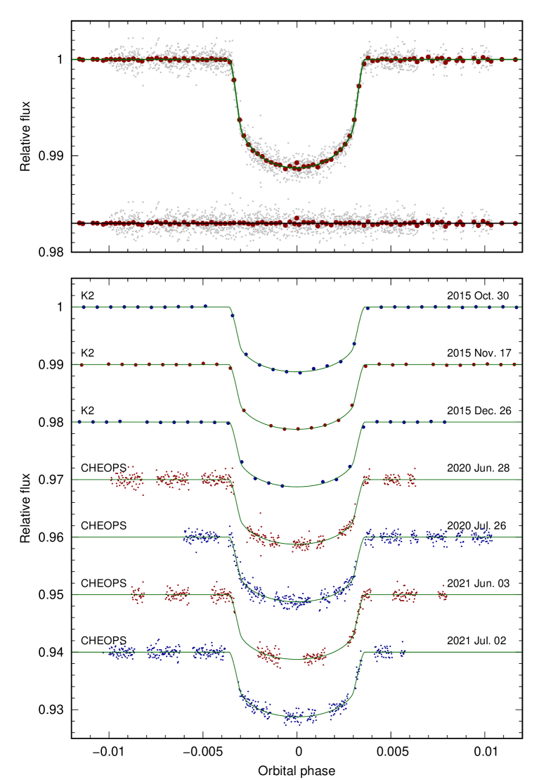
Figure 3: Transit photometry of K2-139. The top panel shows the combined K2 and CHEOPS light curve, phase folded and with all the systematics and the red-noise wavelets subtracted. The original data points are plotted as small grey points, and the larger red circles are the same data binned in phase, with a bin width corresponding to 10 minutes. Below are the residuals to our best-fitting model. The lower panel shows the individual K2 and CHEOPS light curves, labelled with the corresponding instrument name and the UT date of mid-transit, and vertically offset for clarity. In all cases, our best-fitting model is shown as a solid green line.

A fit with separate limb-darkening parameters for the two instruments results in coefficients for K2 which are compatible with those obtained jointly, but less-precisely determined. Finally, the resulting transit parameters are not affected by our choice to fit for only a single set of limb-darkening coefficients, with the differences between the two parameter sets less than $1\sigma$. The resulting parameters from the joint fit using a common set of limb-darkening coefficients are shown in the final column of Table 4, and the photometry is plotted alongside the best-fitting model in Fig. 3.

4.4 Spot-crossing signal

Unlike the K2 transits, we see no evidence of a spot-crossing signal in any of the CHEOPS transits. In order to be certain that we didn’t miss any such signal, we also looked at the light curves and their residuals produced using each of the four photometric apertures (Sect. 2), fitted both with and without the wavelet red noise model. We also verified that a spot-crossing signal of the type seen in the K2 data would not be removed by our modelling of the systematic noise in the CHEOPS light curves. We did this by modelling the K2 spot-crossing signal with a toy model, and injecting this signal into the CHEOPS light curves, before fitting them with the procedure described above. This injected signal has an amplitude of 800 ppm, and a duration of 120 minutes. For comparison, the longest gap in the CHEOPS light curves is around 50 minutes, with gaps of 20 – 30 minutes more typical. The signal was still visible in the CHEOPS light curves, even after fitting them with the wavelet model. In common with B18, we find that excluding the K2 points affected by the spot crossings results in a change to the transit parameters which is much smaller than the 1 $\sigma$ uncertainties on those parameters. We therefore opt not to exclude these points from the final fit.

4.5 Transit timing

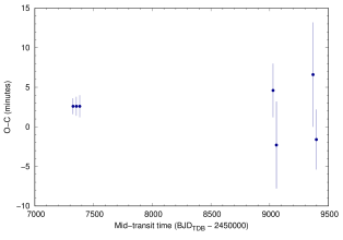
Figure 4: Transit times of K2-139 b. The differences between the observed transit times and our newly-derived ephemeris ($O-C$) are plotted against the mid-transit time (See Table 5).

To measure the time of mid-transit for each of the observed transits of K2-139 b, we re-fit each transit light curve individually, with $P_{\mathrm{orb}}$ fixed to the value of our joint fit, and with priors corresponding to the posterior distribution of our joint fit placed on the other transit parameters. These transit times and their uncertainties are listed in Table 5, where they are also compared to the ephemeris reported by B18, and the ephemeris determined from our joint fit. Although the four CHEOPS transits show significant timing deviation from the B18 ephemeris, this is due to the insufficient precision of the period determined by B18, from just three sparsely-sampled transits. Our newly-determined $P_{\mathrm{orb}}$ is six times more precise, and with this ephemeris, there is no evidence for any significant TTVs – the measured deviations of 2 – 7 minutes from our ephemeris are comparable to the timing precision of 1 – 7 minutes on the individual transits (Fig. 4).

4.6 Orbital eccentricity and stellar density

Alongside the K2 photometry, B18 fitted 19 RV measurements of K2-139, made with three different telescopes / spectrographs. They determined that a simple Keplerian model was a poor fit to the RVs, which are affected by stellar activity. To model this activity, they fit two additional sine curves to the data, at the stellar rotation period and its first harmonic. This fit resulted in a small orbital eccentricity, $e=$$0.12\begin{subarray}{c}+0.12\\ -0.08\end{subarray}$, and a poorly-determined argument of periastron, $\omega=$ $124\begin{subarray}{c}+175\\ -79\end{subarray}$. Since the B18 eccentricity value is consistent with zero at the $2\sigma$ level, and relatively little information about orbital eccentricity is conveyed by transit light curves, we opt to impose a circular orbit solution, by fixing $e=0$.

The stellar density calculated from the mass and radius produced by ariadne is $\mbox{$\rho_{\star}$}=1937\pm 124$ $\mathrm{kg\,m}^{-3}$, whereas the density from our fit to the K2 and CHEOPS transits is $\mbox{$\rho_{\star}$}=2593\pm 211$ $\mathrm{kg\,m}^{-3}$, which differ by around $2.7\sigma$. We therefore tried fitting the light curves again, this time fixing $e$ and $\omega$ to the best-fitting values of B18. All of the resulting parameters and uncertainties are virtually identical to those from the circular orbit fit (with agreements well within $1\sigma$), except we find $a/\mbox{$R_{\star}$}=43.3\begin{subarray}{c}+0.9\\ -1.9\end{subarray}$, which is discrepant from the circular value by $2.4\sigma$. The stellar density calculated with this value of $a/\mbox{$R_{\star}$}$ is $\mbox{$\rho_{\star}$}=1905\pm 183$ $\mathrm{kg\,m}^{-3}$, which is in excellent agreement with the ariadne value. This suggests that the orbit of K2-139 b may indeed be slightly eccentric. We propose that a new RV study of K2-139 is needed to resolve the question of K2-139 b’s orbital eccentricity.

Table 4: Parameters from light curve and RV data analysis.

Parameter	B18	CHEOPS	CHEOPS & K2
Fitted parameters:
Orbital period $P_{\mathrm{orb}}$/ d	$28.38236\pm 0.00026$	$28.38282\pm 0.00016$	$28.382796\pm 0.000042$
Transit epoch $T_{0}$ / BJD${}_{\mathrm{TDB}}-2450000$	$7325.81714\pm 0.00033$	$9057.1673\pm 0.0014$	$9057.16689\pm 0.00083$
Scaled semi-major axis $a/\mbox{$R_{\star}$}$	$44.8\begin{subarray}{c}+4.7\\ -6.7\end{subarray}$	$47.6\begin{subarray}{c}+1.1\\ -2.1\end{subarray}$	$48.0\begin{subarray}{c}+0.9\\ -1.7\end{subarray}$
Radius ratio $\mbox{$R_{\rm p}$}/\mbox{$R_{\star}$}$	$0.0961\begin{subarray}{c}+0.0023\\ -0.0015\end{subarray}$	$0.0955\begin{subarray}{c}+0.0028\\ -0.0026\end{subarray}$	$0.0957\pm 0.0021$
Transit impact parameter $b$	$0.30\begin{subarray}{c}+0.21\\ -0.19\end{subarray}$	$0.16\begin{subarray}{c}+0.18\\ -0.12\end{subarray}$	$0.15\begin{subarray}{c}+0.15\\ -0.11\end{subarray}$
Limb-darkening coefficient‡ $u_{+}$	$0.53\pm 0.25$	$0.64\pm 0.17$	$0.62\pm 0.15$
Limb-darkening coefficient‡ $u_{-}$	$0.47\pm 0.42$	$0.46\pm 0.37$	$0.46\pm 0.37$
Radial velocity semi amplitude $K$ / m s-1	$27.7\begin{subarray}{c}+6.0\\ -5.3\end{subarray}$	–	–
Derived parameters:
Orbital eccentricity $e$	$0.12\begin{subarray}{c}+0.12\\ -0.08\end{subarray}$	0.0 (fixed)	0.0 (fixed)
Argument of periastron $\omega$ / degrees	$124\begin{subarray}{c}+175\\ -79\end{subarray}$	–	–
Semi-major axis $a$ / au	$0.179\begin{subarray}{c}+0.021\\ -0.027\end{subarray}$	$0.1747\pm 0.0016$	$0.1747\pm 0.0016$
Orbital inclination angle $i$ / degrees	$89.62\begin{subarray}{c}+0.25\\ -0.36\end{subarray}$	$89.80\begin{subarray}{c}+0.14\\ -0.23\end{subarray}$	$89.82\begin{subarray}{c}+0.12\\ -0.19\end{subarray}$
Transit Duration $T_{14}$ / h	$4.89\begin{subarray}{c}+0.08\\ -0.22\end{subarray}$	$4.912\begin{subarray}{c}+0.098\\ -0.078\end{subarray}$	$4.891\begin{subarray}{c}+0.084\\ -0.067\end{subarray}$
Planet mass* $M_{\mathrm{p}}/M_{\mathrm{Jup}}$	$0.387\begin{subarray}{c}+0.083\\ -0.075\end{subarray}$	$0.382\pm 0.078$	$0.382\pm 0.078$
Planet radius $R_{\mathrm{p}}/R_{\mathrm{Jup}}$	$0.808\begin{subarray}{c}+0.034\\ -0.033\end{subarray}$	$0.802\begin{subarray}{c}+0.029\\ -0.027\end{subarray}$	$0.803\begin{subarray}{c}+0.024\\ -0.023\end{subarray}$
Planet mean density / kg m-3	$910\begin{subarray}{c}+240\\ -200\end{subarray}$	$912\begin{subarray}{c}+222\\ -206\end{subarray}$	$912\begin{subarray}{c}+212\\ -198\end{subarray}$
Planet equilibrium temperature† $T_{\mathrm{p,A=0}}$ / K	$565\begin{subarray}{c}+48\\ -32\end{subarray}$	$538\begin{subarray}{c}+13\\ -9\end{subarray}$	$536\begin{subarray}{c}+11\\ -8\end{subarray}$

* calculated for the CHEOPS and CHEOPS & K2 columns using the $K$ measured by B18, and the stellar mass from Table 3. ^†assuming zero albedo, and isotropic heat redistribution.

^‡ B18 fit for $q_{1}$ and $q_{2}$, converted here to $u_{+}$ and $u_{-}$ for ease of comparison.

Table 5: Fitted times of mid-transit for individual transits of K2-139 b, their uncertainties (in days and in minutes), and the deviations (O-C) from the ephemerides presented in B18 and our updated ephemeris.

$E$	$T_{\rm c}-2\ 450\ 000$	$\sigma_{T_{\rm c}}$	$\sigma_{T_{\rm c}}$	(O-C) / min
(B18)	$\mathrm{BJD_{TDB}}$	d	min	B18	new $P$
0	7325.8181	0.0007	1.0	1.4	2.6
1	7354.2010	0.0008	1.2	2.1	2.6
2	7382.5837	0.0010	1.4	2.7	2.6
60	9028.7873	0.0024	3.4	41.1	4.6
61	9057.1653	0.0038	5.5	34.9	-2.3
72	9369.3822	0.0046	6.6	50.6	6.6
73	9397.7593	0.0026	3.8	43.1	-1.6

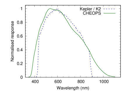
Figure 2: Comparison of Kepler/K2 (dashed line) and CHEOPS (solid line) instrument response as a function of wavelength. The Kepler data are taken from the Kepler Science Center, and the CHEOPS data from the ESA website.

5 Results and discussion

5.1 Updated system parameters and ephemeris

Our combined modelling of the K2 and CHEOPS photometry has resulted in better-determined transit parameters, particularly $a/\mbox{$R_{\star}$}$ and the limb-darkening coefficients, which benefit from the shorter cadence of the CHEOPS observations. The precision in $\mbox{$R_{\rm p}$}/\mbox{$R_{\star}$}$ is, however, not improved by the CHEOPS data. This validates the approach of modelling the long-cadence K2 data using sub-exposures – this technique is still able to measure $\mbox{$R_{\rm p}$}/\mbox{$R_{\star}$}$ with high precision, while measuring $a/\mbox{$R_{\star}$}$ accurately, if somewhat imprecisely.

As expected, our measurement of the orbital period is considerably more precise than that of B18. The 1$\sigma$ uncertainty on the transit time is now around two minutes at the end of 2022, compared to more than 30 minutes previously, and will still be well under 10 minutes at the end of the current decade. Even at the end of the subsequent decade, the uncertainty will only be around 15 minutes, compared to approximately two hours for the B18 ephemeris. This improvement will allow follow-up observations with e.g. Ariel to be planned and executed efficiently.

5.2 Transit timing

As reported in Sect. 4.5 and Table 5, we find no evidence for TTVs. Our individual transit timings from CHEOPS have relatively large uncertainties, which is caused by poor sampling of the ingress and egress phases of the transits. Borsato et al. (2021) measured the transit times of several warm Jupiters with CHEOPS, achieving precisions ranging from around 20 s to about 4 minutes, depending on the brightness of the host star, and the efficiency of the in/egress phases. This range of precision is similar to that achieved by the CoRoT satellite for CoRoT-1b; whose data also suffered from some gaps (Csizmadia et al., 2010). K2-139 is fainter than all of the targets studied by Borsato et al. (2021), and none of our transits has good coverage of both ingress and egress which is needed for the most-precise transit times. Good coverage of both ingress and egress would lead to transit times with a precision of around 30 – 60 s, as measured with CHEOPS for WASP-103 (Barros et al., 2022) which is slightly fainter than K2-139.

The presence of TTVs could be indicative of the presence of a companion planet; warm Jupiters are found to have companions more frequently than hot Jupiters (Huang et al., 2016). A full exploration of the properties of the external perturbers not excluded by our non-detection of TTVs is beyond the scope of this work. We can, however, place indicative upper limits on the maximum allowed mass of a putative outer planet, $M_{\mathrm{c}}$, for a given orbital period, $P_{\mathrm{c}}$, and eccentricity, $e_{\mathrm{c}}$, of the perturber, using Eq. 2 of Holman & Murray (2005):

$$M_{\mathrm{c}}=\frac{16\pi}{45}\mbox{$M_{\star}$}\frac{\Delta t_{\mathrm{max}}}{P_{\mathrm{orb}}}\left(\frac{P_{\mathrm{c}}}{P_{\mathrm{orb}}}\right)^{2}(1-e_{\mathrm{c}})^{3},$$ (2)

where $\Delta t_{\mathrm{max}}$ is the maximum allowed TTV amplitude. We adopt $\Delta t_{\mathrm{max}}=15$ minutes, which is approximately three times the mean uncertainty on the timing of the CHEOPS transits.

In Fig. 5 we plot the maximum allowed perturber mass as a function of orbital period for several values of $e_{\mathrm{c}}$. Our constraints are not particularly strong, but we are able to exclude the presence of a massive planet orbiting with a period less than around 150 days or a brown dwarf with $P_{\mathrm{c}}\lessapprox 1$ yr. Much of the parameter space, however, is not excluded; for instance the outer massive planet (or brown dwarf) in the K2-99 system, which is clearly visible in the RV measurements of the system (Smith et al., 2017, 2022), is only expected to induce TTVs for the inner warm Jupiter with an amplitude of just a few minutes. We would not have detected such a signal in our observations of K2-139, nor would we have detected the outer brown dwarf in the CoRoT-20 system (Deleuil et al., 2012; Rey et al., 2018).

5.3 Starspots

We conclude that there is no evidence for any spot-crossing event in the CHEOPS light curves, which suggests that there were no sufficiently large starspots along the transit chord at the time of these observations. This could be due to chance, or due to the reduced chromospheric activity at a quieter phase of K2-139’s stellar cycle.

Unfortunately this means that we are unable to place any constraint on the obliquity of K2-139 b. Measuring this quantity for warm Jupiters remains very interesting, because the orbital distance of these systems means that their orbits are unlikely to be significantly affected by stellar tidal forces acting to circularize and co-planarize them. This means that an obliquity measurement for K2-139 b would represent the primordial obliquity, following whatever migration processes led the planet to its current orbit. Since different migration processes are expected to result in orbits with different obliquities, measuring this parameter for a sample of warm Jupiters would offer significant insight into migration history. Measuring the obliquity of K2-139 b may be possible via the Rossiter-McLaughlin effect, but any ground-based transit observation of this system is challenging given the lengthy orbital period and transit duration (there is at most one opportunity per year to observe a complete transit of K2-139 b from a given observing site).

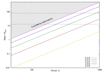
Figure 5: Maximum allowed mass of a perturbing outer body as a function of its orbital period, for different orbital eccentricities of the perturber (solid colored lines). The approximate masses delimiting massive planets from brown dwarfs and brown dwarfs from low-mass stars are indicated with dashed black lines, and the region of parameter space excluded by our TTV observations is shaded.

Appendix A Comparison of limb-darkening coefficients for K2-139

Table 6: Limb-darkening coefficients for K2-139. Values in italics are calculated from coefficients in other forms.

	$u_{a}$	$u_{b}$	$u_{+}$	$u_{-}$
Theoretical Kepler (Claret & Bloemen, 2011)	$0.5256$	$0.1860$	0.7116	0.3396
Theoretical CHEOPS (Claret, 2021)	$0.5419$	$0.1689$	0.7108	0.373
B18 fit to K2 data	0.5$\pm$ 0.24	0.03 $\pm$0.24	0.53 $\pm$ 0.25	0.47 $\pm$ 0.42
Our fit to K2 data only	0.57$\pm$0.17	-0.12$\pm$0.17	$0.45\pm 0.10$	$0.69\pm 0.32$
Our fit to CHEOPS data only	0.55$\pm$0.20	0.09 $\pm$0.20	$0.64\pm 0.17$	$0.46\pm 0.37$
Our fit to K2 & CHEOPS (common l.d.)	0.54$\pm$0.20	0.08 $\pm$0.20	$0.62\pm 0.15$	$0.46\pm 0.37$
Our fit to K2 & CHEOPS (different l.d.): K2	0.35$\pm$0.38	0.22$\pm$0.38	$0.56\pm 0.24$	$0.13\pm 0.72$
Our fit to K2 & CHEOPS (different l.d.): CHEOPS	0.43$\pm$0.34	0.14$\pm$0.34	$0.56\pm 0.22$	$0.29\pm 0.64$

Appendix B Catalog photometry of K2-139 used in the SED fit

Table 7: Catalog photometry of K2-139 used in SED fit.

Band	Magnitude
2MASS $H$	$9.7680\pm 0.0220$
2MASS $J$	$10.1770\pm 0.0220$
2MASS $K_{s}$	$9.6600\pm 0.0230$
Johnson $V$	$11.6780\pm 0.0130$
Johnson $B$	$12.5090\pm 0.0150$
Tycho $B$	$12.6210\pm 0.2050$
Tycho $V$	$11.7400\pm 0.1370$
GaiaDR2 $G$	$11.4626\pm 0.0005$
GaiaDR2 $RP$	$10.8661\pm 0.0017$
GaiaDR2 $BP$	$11.9296\pm 0.0022$
SDSS $g^{\prime}$	$12.0400\pm 0.0050$
SDSS $i^{\prime}$	$11.2250\pm 0.0120$
SDSS $r^{\prime}$	$11.4200\pm 0.0330$
SkyMapper $u$	$13.8500\pm 0.0130$
SkyMapper $v$	$13.4450\pm 0.0090$
SkyMapper $g$	$11.8630\pm 0.0020$
SkyMapper $r$	$11.4550\pm 0.0040$
SkyMapper $i$	$11.1930\pm 0.0030$
SkyMapper $z$	$11.1380\pm 0.0030$
WISE $W1$	$9.6040\pm 0.0230$
WISE $W2$	$9.6770\pm 0.0200$
GALEX (NUV)	$18.3790\pm 0.0610$
TESS	$10.9139\pm 0.0062$

References

- Acton et al. (2020) Acton, J. S., Goad, M. R., Casewell, S. L., et al. 2020, MNRAS, 498, 3115, doi: 10.1093/mnras/staa2513
- Allard et al. (2012) Allard, F., Homeier, D., & Freytag, B. 2012, Philosophical Transactions of the Royal Society A: Mathematical, Physical and Engineering Sciences, 370, 2765, doi: 10.1098/rsta.2011.0269
- Astropy Collaboration et al. (2013) Astropy Collaboration, Robitaille, T. P., Tollerud, E. J., et al. 2013, A&A, 558, A33, doi: 10.1051/0004-6361/201322068
- Barragán et al. (2018) Barragán, O., Gandolfi, D., Smith, A. M. S., et al. 2018, MNRAS, 475, 1765 (B18), doi: 10.1093/mnras/stx3207
- Barros et al. (2022) Barros, S. C. C., Akinsanmi, B., Boué, G., et al. 2022, A&A, 657, A52, doi: 10.1051/0004-6361/202142196
- Benz et al. (2021) Benz, W., Broeg, C., Fortier, A., et al. 2021, Experimental Astronomy, 51, 109, doi: 10.1007/s10686-020-09679-4
- Borkovits et al. (2011) Borkovits, T., Csizmadia, S., Forgács-Dajka, E., & Hegedüs, T. 2011, A&A, 528, A53, doi: 10.1051/0004-6361/201015867
- Borsato et al. (2021) Borsato, L., Piotto, G., Gandolfi, D., et al. 2021, MNRAS, 506, 3810, doi: 10.1093/mnras/stab1782
- Carter & Winn (2009) Carter, J. A., & Winn, J. N. 2009, ApJ, 704, 51, doi: 10.1088/0004-637X/704/1/51
- Castelli & Kurucz (2003) Castelli, F., & Kurucz, R. L. 2003, in Modelling of Stellar Atmospheres, ed. N. Piskunov, W. W. Weiss, & D. F. Gray, Vol. 210, A20. https://arxiv.org/abs/astro-ph/0405087
- Claret (2021) Claret, A. 2021, Research Notes of the American Astronomical Society, 5, 13, doi: 10.3847/2515-5172/abdcb3
- Claret & Bloemen (2011) Claret, A., & Bloemen, S. 2011, A&A, 529, A75, doi: 10.1051/0004-6361/201116451
- Csizmadia (2020) Csizmadia, S. 2020, MNRAS, 496, 4442, doi: 10.1093/mnras/staa349
- Csizmadia et al. (2021) Csizmadia, S., Smith, A. M. S., Cabrera, J., et al. 2021, arXiv e-prints, arXiv:2108.11822. https://arxiv.org/abs/2108.11822
- Csizmadia et al. (2010) Csizmadia, S., Renner, S., Barge, P., et al. 2010, A&A, 510, A94, doi: 10.1051/0004-6361/200912052
- Deleuil et al. (2012) Deleuil, M., Bonomo, A. S., Ferraz-Mello, S., et al. 2012, A&A, 538, A145, doi: 10.1051/0004-6361/201117681
- Deleuil et al. (2018) Deleuil, M., Aigrain, S., Moutou, C., et al. 2018, A&A, 619, A97, doi: 10.1051/0004-6361/201731068
- Dragomir et al. (2020) Dragomir, D., Harris, M., Pepper, J., et al. 2020, AJ, 159, 219, doi: 10.3847/1538-3881/ab845d
- Edwards et al. (2019) Edwards, B., Mugnai, L., Tinetti, G., Pascale, E., & Sarkar, S. 2019, AJ, 157, 242, doi: 10.3847/1538-3881/ab1cb9
- Edwards et al. (2020) Edwards, B., Anisman, L., Changeat, Q., et al. 2020, Research Notes of the American Astronomical Society, 4, 109, doi: 10.3847/2515-5172/aba42b
- Edwards et al. (2021a) Edwards, B., Changeat, Q., Yip, K. H., et al. 2021a, MNRAS, 504, 5671, doi: 10.1093/mnras/staa1245
- Edwards et al. (2021b) Edwards, B., Ho, C. S. K., Osborne, H. L. M., et al. 2021b, arXiv e-prints, arXiv:2111.10350. https://arxiv.org/abs/2111.10350
- Fabrycky & Tremaine (2007) Fabrycky, D., & Tremaine, S. 2007, ApJ, 669, 1298, doi: 10.1086/521702
- Gaia Collaboration et al. (2018) Gaia Collaboration, Brown, A. G. A., Vallenari, A., et al. 2018, A&A, 616, A1, doi: 10.1051/0004-6361/201833051
- Gardner et al. (2006) Gardner, J. P., Mather, J. C., Clampin, M., et al. 2006, Space Sci. Rev., 123, 485, doi: 10.1007/s11214-006-8315-7
- Holman & Murray (2005) Holman, M. J., & Murray, N. W. 2005, Science, 307, 1288, doi: 10.1126/science.1107822
- Howell et al. (2014) Howell, S. B., Sobeck, C., Haas, M., et al. 2014, PASP, 126, 398, doi: 10.1086/676406
- Hoyer et al. (2020) Hoyer, S., Guterman, P., Demangeon, O., et al. 2020, A&A, 635, A24, doi: 10.1051/0004-6361/201936325
- Huang et al. (2016) Huang, C., Wu, Y., & Triaud, A. H. M. J. 2016, ApJ, 825, 98, doi: 10.3847/0004-637X/825/2/98
- Husser et al. (2013) Husser, T.-O., Wende-von Berg, S., Dreizler, S., et al. 2013, A&A, 553, A6, doi: 10.1051/0004-6361/201219058
- Kempton et al. (2018) Kempton, E. M. R., Bean, J. L., Louie, D. R., et al. 2018, PASP, 130, 114401, doi: 10.1088/1538-3873/aadf6f
- Klagyivik et al. (2021) Klagyivik, P., Deeg, H. J., Csizmadia, S., Cabrera, J., & Nowak, G. 2021, Frontiers in Astronomy and Space Sciences, 8, 210, doi: 10.3389/fspas.2021.792823
- Kokori et al. (2021) Kokori, A., Tsiaras, A., Edwards, B., et al. 2021, Experimental Astronomy, doi: 10.1007/s10686-020-09696-3
- Kokori et al. (2022) —. 2022, ApJS, 258, 40, doi: 10.3847/1538-4365/ac3a10
- Kozai (1962) Kozai, Y. 1962, AJ, 67, 591, doi: 10.1086/108790
- Kurucz (1993) Kurucz, R. L. 1993, VizieR Online Data Catalog, 6039
- Lendl et al. (2020) Lendl, M., Csizmadia, S., Deline, A., et al. 2020, A&A, 643, A94, doi: 10.1051/0004-6361/202038677
- Lidov (1962) Lidov, M. L. 1962, Planet. Space Sci., 9, 719, doi: 10.1016/0032-0633(62)90129-0
- Maxted et al. (2021) Maxted, P. F. L., Ehrenreich, D., Wilson, T. G., et al. 2021, MNRAS, doi: 10.1093/mnras/stab3371
- Moutou et al. (2013) Moutou, C., Deleuil, M., Guillot, T., et al. 2013, Icarus, 226, 1625, doi: 10.1016/j.icarus.2013.03.022
- Price-Whelan et al. (2018) Price-Whelan, A. M., Sipőcz, B. M., Günther, H. M., et al. 2018, AJ, 156, 123, doi: 10.3847/1538-3881/aabc4f
- Rasio & Ford (1996) Rasio, F. A., & Ford, E. B. 1996, Science, 274, 954, doi: 10.1126/science.274.5289.954
- Rey et al. (2018) Rey, J., Bouchy, F., Stalport, M., et al. 2018, A&A, 619, A115, doi: 10.1051/0004-6361/201833180
- Ricker et al. (2015) Ricker, G. R., Winn, J. N., Vanderspek, R., et al. 2015, Journal of Astronomical Telescopes, Instruments, and Systems, 1, 014003, doi: 10.1117/1.JATIS.1.1.014003
- Sanchis-Ojeda et al. (2011) Sanchis-Ojeda, R., Winn, J. N., Holman, M. J., et al. 2011, ApJ, 733, 127, doi: 10.1088/0004-637X/733/2/127
- Schlafly & Finkbeiner (2011) Schlafly, E. F., & Finkbeiner, D. P. 2011, Astrophysical Journal, 737, doi: 10.1088/0004-637X/737/2/103
- Schlegel et al. (1998) Schlegel, D. J., Finkbeiner, D. P., & Davis, M. 1998, ApJ, 500, 525, doi: 10.1086/305772
- Smith et al. (2017) Smith, A. M. S., Gandolfi, D., Barragán, O., et al. 2017, MNRAS, 464, 2708, doi: 10.1093/mnras/stw2487
- Smith et al. (2018) Smith, A. M. S., Cabrera, J., Csizmadia, S., et al. 2018, MNRAS, 474, 5523, doi: 10.1093/mnras/stx2891
- Smith et al. (2021) Smith, A. M. S., Acton, J. S., Anderson, D. R., et al. 2021, A&A, 646, A183, doi: 10.1051/0004-6361/202039712
- Smith et al. (2022) Smith, A. M. S., Breton, S. N., Csizmadia, S., et al. 2022, MNRAS, 510, 5035, doi: 10.1093/mnras/stab3497
- Southworth (2011) Southworth, J. 2011, MNRAS, 417, 2166, doi: 10.1111/j.1365-2966.2011.19399.x
- Tinetti et al. (2018) Tinetti, G., Drossart, P., Eccleston, P., et al. 2018, Experimental Astronomy, 46, 135, doi: 10.1007/s10686-018-9598-x
- Vines & Jenkins (2022) Vines, J. I., & Jenkins, J. S. 2022, MNRAS, doi: 10.1093/mnras/stac956
- Weidenschilling & Marzari (1996) Weidenschilling, S. J., & Marzari, F. 1996, Nature, 384, 619, doi: 10.1038/384619a0